ABSTRACT

Title of thesis: SCHEDULING IN ENERGY HARVESTINGSYSTEMS WITH HYBRID ENERGY STORAGE

Khurram Shahzad, Master of Science, 2013

Directed by: Professor Sennur UlukusDepartment of Electrical and Computer Engineering

In wireless networks, efficient energy storage and utilization plays a vital role,

resulting in a prolonged lifetime and enhanced throughput. This factor becomes even

more important in systems employing energy harvesting as compared to utility or

battery powered networks, where a constant supply of energy is available. Therefore,

it is crucial to design schemes that make the best use of available energy resources,

keeping in view the practical constraints.

In this work, we consider data transmission with an energy harvesting trans-

mitter which has hybrid energy storage with a perfect super-capacitor (SC) and an

inefficient battery. The SC has finite storage space while the battery has unlimited

storage space. The transmitter can choose to store the harvested energy in the SC or

in the battery, while draining energy from the SC and the battery simultaneously.

Under this energy storage setup, we solve throughput optimal energy allocation

problem over a point-to-point channel in an offline setting. The hybrid energy stor-

age model with finite and unlimited storage capacities imposes a generalized set of

constraints on the transmission policy. We show that the solution is found by a

sequential application of the directional water-filling algorithm.

Next, we consider offline throughput maximization in the presence of an ad-

ditive time-linear processing cost in the transmitter’s circuitry. In this case, the

transmitter has to additionally decide on the portions of the processing cost to be

drained from the SC and the battery. Despite this additional complexity, we show

that the solution is obtained by a sequential application of a directional glue-pouring

algorithm, parallel to the costless processing case. Finally, we provide numerical il-

lustrations for optimal policies and performance comparisons with some heuristic

online policies.

SCHEDULING IN ENERGY HARVESTING SYSTEMSWITH HYBRID ENERGY STORAGE

by

Khurram Shahzad

Thesis submitted to the Faculty of the Graduate School of theUniversity of Maryland, College Park in partial fulfillment

of the requirements for the degree ofMaster of Science

2013

Advisory Committee:Professor Sennur Ulukus, Chair/AdvisorProfessor Gang QuProfessor Alireza Khaligh

c© Copyright byKhurram Shahzad

2013

To my parents,

Whose love and support means the world to me.

ii

Acknowledgments

All thanks to Almighty ALLAH for giving me the strength and knowledge for

the completion of this work.

I would like to thank my supervisor Professor Sennur Ulukus, for giving me

the opportunity to work with her, which made this thesis possible. I thank her for

putting her trust in me, even when at times I gave no reason at all. She has always

been supportive of my work and her availability made things simple and easy for

me. She always listened to me with a smiling face and let me pursue my ideas.

Working with her was a great learning experience and I benefited immensely from

her vast knowledge.

I thank Professor Gang Qu and Professor Alireza Khaligh for agreeing to serve

on my thesis committee. I thank them for their valuable guidance and helping me

shape the thesis in the final stages. Special thanks to Professor Alireza Khaligh

for the discussions regarding the implementation and practical significance of the

present work. A special thanks is due to Omur Ozel for all his help and encourage-

ment over the course of this work. He not only listened to my often absurd ideas

with patience but also guided me in the right direction. I wish him all the best for

his future.

During my stay in the US, I made some great friends who made this journey

both memorable and enjoyable. I thank Waseem Malik for all the support during

these years. He made me realize how things can change and remain the same at

the same time. I thank Sangjin Han and Jorgos Zoto for all the great times. They

iii

strengthened the emotion that friendship is free from the religious and geographical

boundaries. A special thanks to Sangjin Han for being there for me and listening

to me whenever I felt under the weather. Also I enjoyed his new ride as much as he

did. I thank Jorgos for being there for me in difficult times. I wish them both the

best of everything. I would like to thank Vaibhav Singh and Krishna Puvvada for

their company, support and providing me with really enjoyable times. I also thank

Himanshu Tyagi and Siddharth Pal for their friendship.

Thanks are due to Waqas Ahmed and his loving family for providing me a

home away from home. He is not only among the best friends I have but also an

elder brother without whose help things would have been very difficult for me here

in the US. I would like to take this opportunity to thank IIE, USEFP and Fulbright

organization for providing the means for me to pursue my studies at University of

Maryland. I also thank the staff of ECE department for being helpful over the

course of my studies at UMD.

Finally, I would like to thank my parents and my sisters for their unconditional

and unlimited love and support. I thank my parents for all the sacrifices they have

made for us and for being tireless in providing us. I specially thank my younger

sister Sadia Riaz for being there with my parents and not letting them feel my

absence.

iv

Table of Contents

List of Figures vii

1 Introduction 1

1.1 Energy Harvesting in Wireless Communication . . . . . . . . . . . . . 1

1.2 Energy Storage Technologies . . . . . . . . . . . . . . . . . . . . . . . 3

1.3 Literatue Review and Contribution . . . . . . . . . . . . . . . . . . . 5

2 System Model 10

3 Throughput Maximization with Hybrid Energy Storage Model 14

3.1 Introduction . . . . . . . . . . . . . . . . . . . . . . . . . . . . . . . . 14

3.2 Offline Throughput Maximization . . . . . . . . . . . . . . . . . . . . 15

3.2.1 Optimal Policy for Fixed δi = 0 . . . . . . . . . . . . . . . . . 20

3.2.2 Determining Optimal δ∗i . . . . . . . . . . . . . . . . . . . . . 23

3.2.3 Discussion . . . . . . . . . . . . . . . . . . . . . . . . . . . . . 26

3.3 Conclusion . . . . . . . . . . . . . . . . . . . . . . . . . . . . . . . . . 27

3.4 Appendix . . . . . . . . . . . . . . . . . . . . . . . . . . . . . . . . . 28

3.4.1 Proof of Lemma 3.2.5 . . . . . . . . . . . . . . . . . . . . . . . 28

4 Hybrid Energy Storage with Non-Ideal Processing Power 31

4.1 Introduction . . . . . . . . . . . . . . . . . . . . . . . . . . . . . . . . 31

4.2 Offline Throughput Maximization . . . . . . . . . . . . . . . . . . . . 32

4.2.1 The Case of a Single Epoch . . . . . . . . . . . . . . . . . . . 32

4.2.2 The Case of Multiple Epochs . . . . . . . . . . . . . . . . . . 36

4.2.3 Optimal Policy for Fixed δi = 0 . . . . . . . . . . . . . . . . . 41

4.2.4 Determining Optimal δ∗i . . . . . . . . . . . . . . . . . . . . . 42

4.3 Conclusion . . . . . . . . . . . . . . . . . . . . . . . . . . . . . . . . . 46

v

4.4 Appendix . . . . . . . . . . . . . . . . . . . . . . . . . . . . . . . . . 48

4.4.1 Proof of Lemma 4.2.4 . . . . . . . . . . . . . . . . . . . . . . . 48

5 Numerical Results and Simulations 51

5.1 Deterministic Energy Arrivals . . . . . . . . . . . . . . . . . . . . . . 51

5.2 Stochastic Energy Arrivals . . . . . . . . . . . . . . . . . . . . . . . . 53

6 Conclusions 60

Bibliography 62

vi

List of Figures

2.1 System model with hybrid energy storage. . . . . . . . . . . . . . . . 11

3.1 The variables in the original problem formulation and its equivalent

formulation followed in this thesis. . . . . . . . . . . . . . . . . . . . . 16

3.2 An example of optimal power allocation for δi = 0. . . . . . . . . . . 22

3.3 Transforming the directional water-filling setting. . . . . . . . . . . . 24

3.4 The water flow in the transformed directional water-filling setting. . . 25

4.1 Optimal allocation with δi = 0. . . . . . . . . . . . . . . . . . . . . . 43

4.2 Determining δi in the transformed setting. . . . . . . . . . . . . . . . 45

4.3 Demonstration of water backflow and energy meters. . . . . . . . . . 46

5.1 Optimal transmit powers for hybrid storage with E = [4, 4, 5, 2, 3] mJ

at times t = [2, 3, 8, 9] sec, η = 0.75, Emax = 5 mJ and T = 10 sec. . . 52

5.2 Optimal transmit powers for E = [4, 7, 3, 5, 1, 8, 6] mJ at times t =

[2, 3, 5, 8, 9, 10] sec, η = 0.75, Emax = 5 mJ, ǫ = 1 and T = 12 sec. . . 53

5.3 Performances of the proposed policies for varying energy arrival rates

λ with η = 0.6, Emax = 2 mJ and T = 10 sec. . . . . . . . . . . . . . 55

5.4 Performances of the proposed policies for varying transmission dead-

line constraint T with η = 0.6, Emax = 1 mJ and λ = 1 mJ/sec. . . . 57

5.5 Performances of the proposed policies for varying battery efficiency η

with Emax = 1 mJ, λ = 1 mJ/sec and T = 10 sec. . . . . . . . . . . . 57

5.6 Performances of the proposed policies for varying energy arrival rates

λ with non-ideal processing power using η = 0.6, Emax = 2 mJ, ǫ = 1

mJ/sec and T = 10 sec. . . . . . . . . . . . . . . . . . . . . . . . . . 58

vii

5.7 Performances of proposed policies for varying deadline constraint T

with non-ideal processing power using η = 0.6, Emax = 1 mJ, ǫ = 1

mJ/sec and λ = 1 mJ/sec. . . . . . . . . . . . . . . . . . . . . . . . . 59

viii

Chapter 1

Introduction

1.1 Energy Harvesting in Wireless Communication

Energy concerns in wireless communication networks have recently gained a

considerable attention from the research community [1]. Energy-limited wireless sys-

tems e.g., wireless sensor networks, are equipped with fixed energy supply devices

such as batteries which possess limited operation time and energy. For applications

where replacing the energy source is cumbersome, unaffordable or some times even

impossible, e.g., in unsafe and toxic environments, energy harvesting (EH) appears

as a reasonable solution for safe and unlimited energy supply to communication net-

works. Environmental energy harvesting has been recently considered for improving

the sustainable lifetimes of systems e.g., wearable computers and sensor networks

etc. Numerous harvesting approaches have been successfully demonstrated including

wind, solar, vibrational, biochemical, and motion based, and several others are cur-

rently being developed [2,3]. The amount of energy captured from the environment

is highly dependent on the energy source. Power densities of different harvesting

technologies are shown in Table 1.1 [2].

In energy harvesting wireless systems, energy acquired for data transmission

is incrementally harvested from the environment during the data transmission as

the energy producing phenomena is not always present. Moreover, energy is first

1

Table 1.1: Power Densities of Harvesting Technologies

Harvesting Technology Power Density

Solar Cells (outdoors at noon) 15mW/cm3

Piezoelectric (shoe inserts) 330µW/cm3

Vibration (small microwave oven) 116µW/cm3

Thermoelectric (10C Gradient) 40µW/cm3

Acoustic Noise (100dB) 960nW/cm3

saved in an energy storage unit before it is used for data transmission and unused

energy remains in the storage unit for future use. In order to obtain best utility for

this unlimited, time-varying and uncontrollable source of energy, energy consump-

tion has to be carefully managed according to the times and amounts of energy

harvests and the rate of data transmission must be adapted accordingly. One of

the key parameters that determine a system’s lifetime and hence performance is the

efficiency with which the harvested energy is stored and utilized. This is especially

important in a distributed harvesting system, such as a sensor network, where each

node may have different environmental harvesting opportunities and hence, instead

of just minimizing the total energy consumption, it becomes necessary to adapt

the power management scheme to account for these spatio-temporal variations [2].

In this regard, a few energy-aware designs and aspects of energy management in

sensor networks are discussed in [4], while a game theoretic approach to energy

management in sensor networks is described in [5].

2

1.2 Energy Storage Technologies

Energy storage design is, possibly, one of the most complex design aspect in an

energy harvesting system. Commonly used options for energy storage are batteries

and Electric Double Layer Capacitor (EDLC), also known as super-capacitor (SC).

Both of these storage choices offer their own benefits and limitations. EDLC uses

carbon as the electrodes and stores charge in the electric field at the interface using

aqueous or non-aqueous electrolyte. The charging of EDLC is a purely physical

phenomena rather than a chemical reaction and hence highly reversible process,

which results in high cycle life, long shelf life and a maintenance-free product. Some

of the advantages that the EDLC offers are [6]:

• Unlimited charge cycle life

• High power density

• No thermal heat during discharge

• No risk of overcharging

• Unaffected by deep discharges

• Longer lifetime

• Operating temperature range as great as between −50oC to 85oC

However supercapacitors involve intrinsic leakage due to parasitic paths in the

external circuitry [7, 8], which precludes their use for long term energy storage [2].

Batteries, as compared to supercapacitors are a relatively mature technology and

have a higher energy density. Different kinds of rechargeable batteries are used in

3

EH applications including Nickel Cadmium (NiCd), Nickel Metal Hydride (NiMH),

Lithium based (Li), and Sealed Lead Acid (SLA). Of these, SLA and NiCD batteries

are less used because of relatively low energy density and temporary capacity loss

caused by shallow discharge cycles, termed as the memory effect. The choice between

NiMH and Li batteries involves several tradeoffs. Li batteries are more efficient

than NiMH, have a longer cycle lifetime, and involve a lower rate of self-discharge.

However, they are more expensive, even after accounting for their increased cycle

life. Li batteries also require a significantly more complicated charging circuit [2].

Although batteries do offer high energy densities but the lack of high power

densities sometimes makes them unsuitable for applications where instantaneous

power transmissions are required as is typical of sensor networks. On the other

hand, supercapacitors suffer from low energy densities and thus cannot work as

a standalone unit for energy storage. Tiered energy storage mechanisms using a

combination of supercapacitor and batteries have been proposed in the literature for

similar applications [9–11] to achieve a better overall performance. This combination

has been advocated to inherently offer better performance in comparison to the

use of either of them alone. In this thesis, we consider throughput optimal energy

allocation for energy harvesting transmitters with such a hybrid energy storage unit.

In data transmission with such a device, aside from determining the transmit

power level, the transmitter has to decide the portions of the incoming energy to

be saved in the SC and the battery. While it is desirable to save incoming energy

in the SC due to its perfect storage efficiency, the storage capacity limitation neces-

sitates careful management of the energy saved in this device. In this regard, the

4

transmitter may wish to save energy in the inefficient battery rather than losing it.

Therefore, the extra degree of freedom to choose the portions of incoming energy

to save in different storage units significantly complicates the energy management

problem.

1.3 Literatue Review and Contribution

We utilize the offline nature of the work where we assume that the transmitter

knows exactly the amount and time of energy arrivals in advance. Offline through-

put maximization for energy harvesting systems has recently received considerable

interest [12–28]. In [12], the transmission completion time minimization problem

is solved in energy harvesting systems with an unlimited capacity battery that op-

erates over a static channel. The solution of this problem has later been extended

for a finite capacity battery [13], fading channel [14], broadcast channel [15–17],

multiple access channel [18], interference channel [19] and relay channel [20,21]. Of-

fline throughput maximization for energy harvesting systems with leakage in energy

storage were studied in [22]. In [23–25], offline optimal performance limits of multi-

user wireless systems with energy transfer are studied. Finally, [28] considers offline

throughput maximization for energy harvesting devices in the presence of energy

storage losses.

As emphasized in [12–28], energy arrivals impose causality constraints on

the energy management policy. In addition, battery limitation imposes no-energy-

overflow constraints [13, 14, 16]. As the rate-power relation is concave, energy allo-

5

cation has to be made as constant as possible in time subject to the energy causality

and no-energy-overflow constraints. In the presence of hybrid energy storage, the

energy causality and no-energy-overflow constraints take a new form since the trans-

mitter has to govern the internal energy dynamics of the storage unit in addition to

the power levels drained from these devices. We capture the inefficiency of the bat-

tery by a factor η and solve the resulting offline throughput maximization problem.

Although previous work on offline throughput maximization did not address

this more realistic energy storage model, a hybrid storage model has appeared in

[29]. In this work, the authors analyze a save-then-transmit protocol in energy

harvesting wireless systems with a hybrid storage model that operates over fading

channels. The optimal save ratio that minimizes outage probability is derived and

some useful guidelines are given. Our work is different from [29] in that our objective

is throughput maximization and we perform the optimization over a sequence of

variables. Moreover, unlike the hybrid storage model in our work, both of the

storage devices have unlimited capacities in the model of [29].

A natural way of formulating this problem for the specified model is over the

energies drained from the SC and the battery and the portion of the incoming energy

to be saved in the SC. Instead, in the spirit of [30], we formulate the problem in

terms of energies drained from the SC and the battery and energy transferred from

the SC to the battery after initially storing all incoming energy in the SC as much

as possible. This formulation reveals many commonalities of this problem with the

previous works. This problem relates to sum-throughput maximization in a multiple

access channel with energy harvesting transmitters [18] since energies drained from

6

two queues contribute to transmission of a common data. Battery storage loss model

is reminiscent of that in [28] where the transmitter is allowed to save the incoming

energy in a lossy battery or use it immediately for data transmission. Finally, one-

way energy transfer from the SC to the battery relates to the problem considered

in [24] where a two-user multiple access channel is considered with energy transfer

from one node to the other.

Despite the coupling between the variables that represent energies drained

from and transferred within the energy storage unit, we show that the problem can

be solved by application of directional water-filling algorithm [14] in multiple stages.

In particular, we first forbid energy transfer from the SC to the battery and solve this

restricted optimization problem. We show that this problem is solved by optimizing

the SC allocation first and then the battery allocation given the SC allocation. Next,

we allow energy transfer from the SC to the battery and show that the optimal

allocation is obtained by directional water-filling in a setting transformed by the

storage efficiency η. As a consequence, we obtain a generalization of the directional

water-filling algorithm which yields useful insight on the structure of the optimal

offline energy allocation in energy harvesting systems. Byproducts of this analysis

are new insights about the optimal policies over the multiple access channel under

finite battery constraints.

In the second part of the thesis, we extend the offline throughput maximization

problem to the case where a time-linear additive processing cost is present in the

data transmission circuitry. It is well-known that circuit power consumption is non-

negligible compared to the power spent for data transmission in small scale and short

7

range applications [31]. We note that a considerable portion of energy harvesting

communication applications falls into this category, and the effects of circuit power

have been investigated in previous works on energy harvesting communications [26,

27,32,33]. Among these works, the framework that is most pertinent to ours has been

proposed in [27]. In contrast to [27], in our case, the transmitter has to additionally

decide the portions of the energy cost drained from the SC and the battery in the

presence of hybrid energy storage. Despite this additional complexity, we show that

the solution of the throughput maximization problem with hybrid energy storage is

obtained by a sequential application of an extended version of the directional glue

pouring algorithm in [27]. To this end, we first construct an equivalent single epoch

problem by introducing new time and power variables. In particular, we divide the

available time for the SC and the battery and enforce SC and the battery to pay the

energy cost in the corresponding time intervals. Moreover, we allow to drain energy

from the SC only in its time interval while battery energy can be drained in both

intervals. We show that this specific scheme yields a jointly optimal transmission

and energy cost drainage scheme. We, then, generalize the single epoch analysis

to multiple epochs and obtain an extension of the framework in [27] to the case of

hybrid energy storage.

Rest of the thesis is organized as follows. Chapter 2 introduces our hybrid

energy storage system model. Mathematical notations and basic constraints on

the optimization problem are described. Chapter 3 considers the throughput max-

imization problem in the given setup. Chapter 4 extends the work of Chapter 3

to include the processing power overhead. In both these chapters, optimal policies

8

are described in terms of transmit powers keeping in view the system constraints.

In Chapter 5, we illustrate the optimal policies with and without processing cost

in specific numerical studies and provide performance comparisons with heuristic

policies in the online regime. Finally, Chapter 6 concludes the thesis.

9

Chapter 2

System Model

We consider a single-user additive white Gaussian noise (AWGN) channel

where the transmitter is equipped with the energy harvesting capability. The trans-

mitter has three buffers: two energy storing buffers and one buffer for storing the

data to be transmitted. We assume that the transmitter always has data to trans-

mit, hence an infinite backlog. The two energy buffers represent the hybrid storage

system, one for the SC and one for the battery as shown in Fig. 2.1. The SC has

a finite storage capacity and can store Emax units of energy at maximum. The

battery, on the other hand, can store infinite energy but it comes at the cost of

storage inefficiency i.e., a certain portion of the stored energy is lost and a fraction

is available for use.

The physical channel’s input-output model is given by y =√hx+N , where x

and y represent the input and output of the channel respectively, h is the squared

channel gain and N is Gaussian noise with zero-mean and unit-variance. Without

loss of generality, we set h = 1 throughout the communication. We assume that the

transmitter can adjust its power and data rate at will, thus following a continuous

time model. The instantaneous data rate is given by

r(t) =1

2log(1 + p(t)) (2.1)

10

Figure 2.1: System model with hybrid energy storage.

The function r(.) is non-negative, strictly increasing, continuously differen-

tiable and strictly concave, thus for a fixed amount of energy, the number of bits

that can be transmitted increases as the transmission duration increases [12]. At

time tei , Ei amount of energy arrives. Eb0 and Esc

0 amounts of energies are available

at the beginning in the battery and in the SC, respectively. In the following, we

refer to the time interval between two energy arrivals as an epoch. More specifically,

epoch i is the time interval [tei , tei+1) and the length of the epoch i is ℓi = tei+1 − tei .

Whenever energy Ei arrives at time tei , the transmitter stores Esci amount in

the SC and Ebi = Ei −Esc

i amount in the battery. Since SC can store at most Emax

units of energy, Esci must be chosen such that no energy unnecessarily overflows.

For this reason, Esci ≤ Emax must necessarily be satisfied. The efficiency of the

battery is given by the parameter η where 0 ≤ η < 1: If Ebi units of energy is

stored in the battery, then ηEbi units can be drained and (1 − η)Eb

i units are lost.

Moreover, we assume that the available energy in the battery can be transferred

11

to SC instantaneously1. As a consequence, none of the arrived energy overflows;

however, there is an energy loss due to inefficiency of the battery.

We assume a simple form of circuitry power consumption i.e., a constant circuit

power ǫ is consumed whenever the transmitter is in active mode. This constant

power represents the energy consumed by the transmitter hardware including power

amplifiers, active filters and synthesizers and is assumed to be independent of the

level of transmit power [31]. We also assume that the transmitter does not consume

any energy while switching between states. Thus when the processing power is non-

negligible, the power consumption is pi + ǫ in epoch i whenever the transmitter is

in active state and 0 when transmitter is inactive. Due to the presence of ǫ, the

nature of the transmitter becomes bursty i.e., to transmit in a certain fraction of

the available time and stay inactive for rest of the time slot.

A transmit power policy is denoted as p(t) over [0, T ]. p(t) is constrained by

the energy that can be drained from the hybrid storage system:

∫ tei

0

p(u)du ≤i−1∑

j=0

Escj + ηEb

j , ∀i (2.2)

where tei in the upper limit of the integral is considered as tei −ε for sufficiently small

ε.

Moreover, we note that the power policy should cause no energy overflow in the

SC. In order to express this constraint, we divide each incremental drained energy

p(u)du as a linear combination of the energy drained from the SC, psc(u)du, and the

1In real systems, switching time between the battery and the SC is very small compared toepoch lengths of interest [2].

12

energy drained from the battery, pb(u)du. That is, p(u)du = psc(u)du+pb(u)du. We

are allowed to divide p(u)du into such components since the energy in the battery

can be instantaneously transferred to the SC. No-energy-overflow constraint in the

SC can now be expressed as follows:

i∑

j=0

Escj −

∫ tei

0

psc(u)du ≤ Emax, ∀i (2.3)

We note that the constraints in (2.2) and (2.3) generalize the energy causality and

no-energy-overflow constraints in the single-stage energy storage models studied,

e.g., in [14].

13

Chapter 3

Throughput Maximization with Hybrid Energy Storage Model

3.1 Introduction

A key determinant of the performance of energy management policies in en-

ergy harvesting systems is the efficiency of energy storage. In order to use the

harvested energy for data transmission, energy has to be saved in an energy storage

unit, which may foster imperfections such as leakage of the available energy and in-

efficiency due to other physical reasons. In some energy harvesting systems, energy

storage units possess a hybrid storage composed of perfectly efficient and inefficient

components with storage capacity limitations [30]. The extra degree of freedom to

choose to save energy in different storage units significantly complicates the energy

management problems in such systems. While it is desirable to save incoming energy

in perfectly efficient storage device, the storage capacity limitation on this device

necessitates careful management of the energy saved in this device and save energy

in the inefficient one rather than loosing it.

Although the variables in the problem are highly coupled, we show that the

problem is solved by a multi-stage algorithm that involves repeated application of

the directional water-filling algorithm [14]. The solution generalizes the directional

water-filling algorithm for a single stage energy storage and yields valuable insight

on the structure of the optimal energy allocation.

14

3.2 Offline Throughput Maximization

Our objective is to determine the optimal offline schedule for determining the

portions of energies that are stored in the SC and the battery and resulting power

policy that maximizes throughput by a deadline T . The power policy p(t) has to

be constant over each epoch, due to the concavity of the rate-power relation in

(2.1). Therefore, the power policy is represented by the sequence pi = psci + pbi

where psci and pbi are the portions of the power drained from the SC and the battery,

respectively, in epoch i. We note that it suffices to assume constant portions psci

and pbi over epoch i; however, time-varying f sci (t) and f b

i (t) with pi = f sci (t) + f b

i (t)

for all t ∈ [tei , tei+1) and

∫ tei+1

teif sci (t)dt = psci ,

∫ tei+1

teif bi (t)dt = pbi would have the same

performance as well. Moreover, the transmitter decides the portions of the incoming

energy Esci and Eb

i where Esci +Eb

i = Ei. Since the battery is inefficient (0 ≤ η < 1),

we prefer to initially allocate incoming energy to the SC and the remaining energy

to the battery while still allowing to transfer a portion of the energy in SC to the

battery. We denote the energy transfer power at epoch i as δi with the convention

that the transferred energy becomes available for use in epoch i+ 1. The variables

in the original problem formulation and its equivalent formulation are depicted in

Fig. 3.1.

15

Battery

(a) Original formulation (b) Equivalent formulation

SC SCBattery

pbi psc

ipscipb

i

Ei

Esci

Emax

Ei

Esci = min{Ei,Emax}

δi

Emax

Figure 3.1: The variables in the original problem formulation and its equivalentformulation followed in this thesis.

In view of (2.2)-(2.3), we get the following constraints for all i:

i∑

j=1

(

pscj ℓj + δjℓj)

≤i−1∑

j=0

Escj (3.1)

i∑

j=0

Escj −

i∑

j=1

(

pscj ℓj + δjℓj)

≤ Emax (3.2)

i∑

j=1

pbjℓj ≤i−1∑

j=0

(

ηEbj + ηδjℓj

)

(3.3)

psci ≥ 0, pbi ≥ 0, δi ≥ 0 (3.4)

where Esci = min{Ei, Emax} and Eb

i = (Ei − Emax)+. We set δ0 = 0 and δN = 0

by convention. We remark that in the system model, energy transfer from SC to

the battery is not allowed. However, due to the offline nature, we have the freedom

to allocate energy to SC first and then transfer it to the battery. Moreover, one

epoch delay in this energy transfer emphasizes the fact that if the energy in the SC

in epoch i is transferred to the battery, that energy must be utilized starting from

16

epoch i + 1 as otherwise such an energy transfer cannot increase the throughput

since the battery is inefficient.

Offline throughput maximization problem by deadline T with hybrid energy

storage unit is:

maxpsci ,pbi ,δi≥0

N∑

i=1

ℓi2log(

1 + psci + pbi)

s.t. (3.1)− (3.4) (3.5)

We note that the problem in (3.5) is a convex optimization problem and we can

solve it using standard techniques [34]. In fact, the problem in (3.5) is equivalent

to sum-throughput maximization in a multiple access channel where battery of one

of the users has finite capacity while the other has infinite capacity and one-way

energy transfer from the user with finite capacity battery to the other is allowed. A

simpler version of this problem is addressed in [24] where both users have unlimited

battery. The Lagrangian function for (3.5) is

L =−N∑

i=1

ℓi2log(

1 + psci + pbi)

+N∑

i=1

λi

(

i∑

j=1

(

pscj ℓj + δjℓj)

−i−1∑

j=0

Escj

)

+N−1∑

i=1

µi

(

i∑

j=0

Escj −

i∑

j=1

(

pscj ℓj + δjℓj)

− Emax

)

+N∑

i=1

νi

(

i∑

j=1

pbjℓj −i−1∑

j=0

(

ηEbj + ηδjℓj

)

)

−N∑

i=0

γiδi −N∑

i=1

ρ1ipsci −

N∑

i=1

ρ2ipbi (3.6)

17

KKT optimality conditions for (3.5) are:

− 1

1 + psci + pbi+

N∑

j=i

λj −N−1∑

j=i

µj − ρ1i = 0, ∀i (3.7)

− 1

1 + psci + pbi+

N∑

j=i

νj − ρ2i = 0, ∀i (3.8)

N∑

j=i

λj −N−1∑

j=i

µj − ηN∑

j=i+1

νj − γi = 0, ∀i (3.9)

and the complementary slackness conditions are:

λi

(

i∑

j=1

(

pscj ℓj + δjℓj)

−i−1∑

j=0

Escj

)

= 0, ∀i (3.10)

µi

(

i∑

j=0

Escj −

i∑

j=1

(

pscj ℓj + δjℓj)

− Emax

)

= 0, ∀i (3.11)

νi

(

i∑

j=1

pbjℓj −i−1∑

j=0

(

ηEbj + ηδjℓj

)

)

= 0, ∀i (3.12)

γiδi = ρ1ipsci = ρ2ip

bi = 0, ∀i (3.13)

We remark that the optimization problem (3.5) may have many solutions. In order

to get a solution, it suffices to find power sequences psci , pbi and Lagrange multipliers

that are consistent with (3.7)-(3.9) and (3.10)-(3.13). We observe properties of an

optimal solution psc∗i , pb∗i and δ∗i in the following lemmas. We assume η < 1 as for

η = 1, there is no cost incurred due to saving energy in the battery and therefore

energy can be blindly saved in the SC or the battery, yielding a single energy storage

with unlimited space for which the solution is well known [14].

Lemma 3.2.1 If pb∗i 6= 0, psc∗i + pb∗i does not decrease in the passage from epoch i

18

to epoch i+ 1.

Proof: If pb∗i 6= 0, then ρ2i = 0. By (3.8), we have psc∗i + pb∗i = 1∑N

j=i νj− 1 and

psc∗i+1+pb∗i+1 =1

∑Nj=i+1 νj−ρ2(i+1)

−1. Since νi ≥ 0 and ρi+1 ≥ 0, we conclude the desired

result. �

Lemma 3.2.2 If Ebi−1 6= 0, pb∗i = 0 and pb∗i+1 6= 0, then psc∗i + pb∗i does not increase

in the passage from epoch i to epoch i + 1. Similarly, if Ebi−1 = 0, Eb

i = 0, pb∗i = 0

and pb∗i+1 6= 0, then psc∗i + pb∗i does not increase in the passage from epoch i to epoch

i+ 1.

Proof: As pb∗i = 0 and pb∗i+1 6= 0, we have ρ2i ≥ 0 and ρ2(i+1) = 0. Moreover,

since pb∗i = 0, νi = 0 as the constraint∑i

j=1 pbjℓj ≤

∑i−1j=0

(

ηEbj + ηδjℓj

)

cannot

be satisfied with equality when Ebi−1 6= 0 and pb∗i = 0. Similarly, we note that if

Ebi−1 = 0, Eb

i = 0, then∑i

j=1 pbjℓj ≤ ∑i−1

j=0

(

ηEbj + ηδjℓj

)

cannot be satisfied with

equality when pb∗i = 0 and pb∗i+1 6= 0. Therefore,∑N

j=i νj − ρ2i ≤∑N

j=i+1 νj − ρ2(i+1),

which by (3.8) implies the desired result. �

Lemma 3.2.3 If psc∗i , pb∗i 6= 0, then δ∗i = 0.

Proof: If psc∗i , pb∗i 6= 0, from (3.7) and (3.8), we have∑N

j=i λj −∑N−1

j=i µj =∑N

j=i νj.

Combining this with (3.9), we conclude that γi = νi+(1−η)∑N

j=i+1 νj > 0 as η < 1.

In view of the slackness condition γiδi = 0, we get δ∗i = 0. �

Lemma 3.2.4 If psc∗i , psc∗i+1, pb∗i+1 6= 0, psc∗i + pb∗i ≤ psc∗i+1 + pb∗i+1, then δ∗i = 0.

Proof: As psc∗i , psc∗i+1, pb∗i+1 6= 0, ρ1i = ρ1(i+1) = ρ2(i+1) = 0. Therefore, by (3.7) and

19

since psc∗i + pb∗i ≤ psc∗i+1+ pb∗i+1, we have∑N

j=i λj −∑N−1

j=i µj >∑N

j=i+1 λj −∑N−1

j=i+1 µj.

Moreover, since ρ2(i+1) = 0, we have∑N

j=i+1 λj −∑N−1

j=i+1 µj =∑N

j=i+1 νj. By (3.9),

γi > 0 and due to the slackness condition γiδi = 0, we get δ∗i = 0. �

Lemmas 3.2.1-3.2.4 reveal several useful properties of the optimal power se-

quences psc∗i and pb∗i and their relation to the transfer power δ∗i . In view of these

lemmas, we adopt the following strategy: Initially, we fix δi = 0 and find the optimal

policy under this constraint. Note that δi = 0 is a good candidate for an optimal

selection in view of Lemmas 3.2.3-3.2.4. If the resulting optimal policy is compatible

with the KKT conditions, then we stop. Otherwise, we carefully update δi so that

the KKT conditions are satisfied.

3.2.1 Optimal Policy for Fixed δi = 0

For fixed δi = 0, the problem becomes maximizing the throughput by the

deadline subject to energy causality and finite SC Emax constraints only:

maxpsci ,pbi≥0

N∑

i=1

ℓi2log(

1 + psci + pbi)

s.t. (3.1)− (3.4)

δi = 0, ∀i (3.14)

where Esci = min{Ei, Emax} and Eb

i = (Ei − Emax)+. We note that (3.14) is

equivalent to sum-throughput maximization in a two-user multiple access chan-

nel with finite and infinite capacity batteries. A simpler version of this problem

where both users have unlimited battery is addressed in [18]. While the problem of

20

sum-throughput maximization has a simple solution when batteries are unlimited by

summing the energies of the users and performing single-user throughput maximiza-

tion [18], the finite battery constraint in (3.14) disables such a simple solution. As

in the general problem in [18], the solution of (3.14) is found by iterative directional

water-filling where infinitely many iterations are required in general.

Next, we show that due to the problem structure, we can find the solution of

(3.14) only in two iterations. Note that the energy arrivals of the storage units are

Esci = min{Ei, Emax} and Eb

i = (Ei − Emax)+: Energy is first allocated to the SC

and the remaining energy is allocated to the battery. This specific way of allocation

allows us to find the solution in two iterations. We state this result in the following

lemma and provide the proof in Appendix 3.4.1.

Lemma 3.2.5 For fixed δi = 0, let psci be the outcome of directional water-filling

given pbi = 0. Let pbi be the outcome of directional water-filling given psci . Then, psci

and pbi are jointly optimal for (3.14).

We note that the claim in Lemma 3.2.5 would not be true if Esci and Eb

i were

allowed to take arbitrary values. Therefore, apart from providing a crucial step

towards finding the solution of (3.5), the optimality result stated in Lemma 3.2.5 is

an interesting case in the two-user multiple access channel with finite and infinite

batteries where the optimal power sequence can be found only in two iterations.

We provide an illustration of the result of two iterations of directional water-

filling in Fig. 3.2 where blue and red waters represent energies in the SC and the

battery, respectively. In this specific example, Esci = Emax only over epochs 1 and

21

ℓ1

OFF OFF OFF OFF OFF

ℓ1

ℓ1

ℓ2 ℓ3 ℓ4 ℓ5 ℓ6

ℓ2 ℓ3 ℓ4 ℓ5 ℓ6

ℓ2 ℓ4 ℓ5 ℓ6

ON ON ON ON ON

OFF OFF OFF OFF OFF

ℓ1 ℓ2 ℓ3 ℓ4 ℓ5 ℓ6

ℓ3

ON ON ON ON ON

Figure 3.2: An example of optimal power allocation for δi = 0.

4. We observe that the red water level is constant over epochs 1 − 3 and epochs

4− 6. Moreover, in view of Lemma 3.2.1, whenever pbi is non-zero total power level

increases. Note that the statement of Lemma 3.2.1, which is originally stated for

the solution of (3.5), is also true for the solution of (3.14). This is due to the fact

that Lemma 3.2.1 follows from the KKT condition in (3.8) and this condition still

holds under the extra constraint δi = 0.

22

3.2.2 Determining Optimal δ∗i

We note that for psci and pbi , there are Lagrange multipliers λi, µi, νi, ρ1i and

ρ2i that are compatible with (3.7) and (3.8). Accordingly, psci and pbi are compatible

with Lemmas 3.2.1-3.2.2. However, it is not clear if there exist γi that are compatible

with (3.9). In fact, if∑N

j=i λj −∑N

j=i+1 µj − η∑N

j=i+1 νj < 0, then such γi do not

exist and if otherwise γi =∑N

j=i λj −∑N

j=i+1 µj − η∑N

j=i+1 νj. In this section, we

propose a method to update the allocations psci and pbi and the Lagrange multipliers

λi, µi, ρ1i, ρ2i that yield δ∗i and corresponding γi so that (3.7)-(3.9) and (3.10)-(3.13)

are satisfied. For ease of exposition, we restrict our treatment in this section to the

case where Eb1 > 0 and Eb

i = 0 for i = 2, . . . , N ; however, the arguments can be

generalized. One can show that in this case, νN > 0 and νi = 0 for i = 1, . . . , N − 1.

Note that if pbi 6= 0 for some i, resulting Lagrange multipliers yield γi ≥

0. In view of the KKT condition (3.9), we transform the directional water-filling

setting as in Fig. 3.3: We multiply the water level and the bottom level by 1ηat

epochs where pbi > 0 and leave other epochs unchanged where the bottom level is

1. Moreover, if γi ≥ 0, we set δ∗i = 0 and transform the water level and the bottom

level of that epoch. At epochs i with γi < 0, we wish to decrease∑N

j=i νj and

increase∑N

j=i λj −∑N−1

j=i µj so that γi approaches zero and resulting allocations

are compatible with (3.7)-(3.9) and (3.10)-(3.13). We next argue that if energy is

transferred from epochs i with γi < 0 in a coordinated fashion, this is possible.

Recall that νN > 0 and νi = 0 for i = 1, . . . , N − 1. We decrease νN and

increase λi, µi and∑N

j=i λj −∑N−1

j=iµj where i is the epoch index with the lowest

23

T

ONONON

T

ONONON

0

0ℓ1 ℓ2 ℓ4

ℓ1 ℓ2 ℓ4

h

ℓ3

ℓ3

γ3 < 0

γ1 > 0

1∑Nj=i λj−

∑Nj=i+1

µj

− 1

1∑N

j=i νj

− 1

1

η∑N

j=i νj

−

1

η

Figure 3.3: Transforming the directional water-filling setting.

∑N

j=i λj −∑N−1

j=i µj. This decreases the power level psci

and increases the battery

power level pbi at all epochs. Therefore, a non-zero energy transfer from epoch i

occurs. As we decrease νN , γi also increases. In particular, γi may change sign

from negative to positive in which case, we make sure that δ∗i = 0 for that epoch

and hence we transform the bottom levels and the water levels for those epochs

as in Fig. 3.3. On the other hand,∑N

j=i λj −∑N−1

j=iµj increases and it may hit

the second lowest∑N

j=i λj −∑N−1

j=i µj. In this case, we start to increase λi, µi and

∑N

j=i λj −∑N−1

j=i µj in both of these epochs.

Note that this procedure corresponds to a coordinated energy transfer: We

start energy transfer from the epoch i with the highest power level psci . In the

transformed setting, as we transfer δi,1ηδi units of water is added to the next epoch

as shown in Fig. 3.4. If the power level of epoch i decreases to the level of the second

highest power psci with γi < 0, then energy is transferred simultaneously from these

24

T

ONONON

0

T

ONONON

0

> 0> 0

> 0> 0

> 0

ℓ1 ℓ2 ℓ4

hη

ℓ3

> 0

ℓ1 ℓ2 ℓ4

hη

ℓ3

+1

ηδ3

−δ3

Figure 3.4: The water flow in the transformed directional water-filling setting.

epochs. Causality conditions may forbid decreasing νN after some level. This way,

all epochs i which have initially γi < 0 are updated so that γi ≥ 0 with γi = 0 if

δi > 0 and (3.7)-(3.9) and (3.10)-(3.13) are satisfied.

Note that when energy is transferred from the SC to the battery in epoch

i, this energy spreads over future epochs i + 1, . . . , N . Moreover, the energy that

was transferred from epochs 1, . . . , i − 1 in the second directional water-filling of

Lemma 3.2.5 given psci may flow back to these epochs. We, therefore, measure the

transferred energy within the battery at each epoch by means of meters and negate

it if energy flows in the opposite direction. This is reminiscent of the meters used

for the two-way channel in [24, 25].

25

3.2.3 Discussion

When δi = 0, in general the first directional water-filling yields a non-monotone

power sequence psci due to finite storage limit Emax. The second directional water-

filling fills the gaps due to non-monotonicity of psci and ameliorates the

non-monotonicity of the total power level psci + pbi . The second stage of the algorithm

further smooths out the non-monotonicity of the total power by transferring energy

from the SC to the battery in epochs where power is sharply high. Therefore, the cu-

mulative effect of the two-stage algorithm is to collectively transfer energy from the

past to the future in both storage devices and make the total power level as constant

as possible subject to energy causality and finite SC capacity limit constraints. The

extent to which this transfer is continued is determined in a transformed directional

water-filling setting where the key parameter is the storage efficiency η.

We remark that for η = 1, the outcome of the algorithm is the same as the

power policy yielded by single-user directional water-filling applied to the energy

arrivals Ei with unlimited battery capacity. This is due to the fact that storing

energy in the battery or the SC does not cause a performance difference in this

case and hence the same performance is achieved if all energy is allocated to the

battery only. We also remark that for η = 0, the algorithm stops after the first

directional water-filling since the battery is never used in this case. Therefore,

the algorithm reduces to the classical directional water-filling with Emax constraint

in [14]. Finally, we remark that even when the energy arrivals are always smaller

than the SC capacity, i.e., even when Ei ≤ Emax for all i, the presence of the

26

battery improves the throughput performance as the battery enables smoothing out

the variations in the transmit power.

3.3 Conclusion

In this chapter, we analyze data transmission with an energy harvesting trans-

mitter that has a hybrid energy storage unit composed of an inefficient battery and a

perfect super-capacitor (SC). We address the offline throughput maximization prob-

lem for such an energy harvesting transmitter. In order to optimize performance,

internal energy dynamics between the two energy storage units has to be properly

adjusted. We utilize the offline nature of the problem and reformulate it in terms

of energies drained from the SC and the battery and energy transferred from the

SC to the battery. In spite of coupling between the variables in this setting, opti-

mal energy management problem is solved using directional water-filling in multiple

stages: First, energy transfer between the two storage elements is fixed to zero and

energies drained from the SC and the battery are determined. Then, energy trans-

fer, if necessary, is determined. This solution generalizes the single stage directional

water-filling algorithm in [14] and provides valuable insight on how energy is spread

in time as equal as possible subject to energy causality and storage limit constraints.

27

3.4 Appendix

3.4.1 Proof of Lemma 3.2.5

To prove the asserted optimality, it suffices to show that for the power levels

psci and pbi , there are Lagrange multipliers λi, µi, νi, ρ1i, ρ2i that are consistent with

(3.7)-(3.8) and (3.10)-(3.13). Note that we ignored (3.9) as δi = 0 fixed. Consider the

first directional water-filling that yields psci > 0 sequence. Let in be the epoch indices

such that Ein = Emax. We remark that the directional water-filling determines the

energy allocation between the epochs i = in, in + 1, . . . , in+1 − 1 independent of the

other epochs. For the sequence psci , i = in, in + 1, . . . , in+1 − 1, there exist λi and µi

such that

1

1 + psci=

in+1∑

k=i

λk −in+1−1∑

k=i

µk (3.15)

Note that since psci > 0, ρ1i = 0. Therefore, for i = in + 1, . . . , in+1 − 1, energy

causality and no-energy-overflow conditions cannot be simultaneously active, im-

plying that λiµi = 0. In particular, psci increases when λi > 0 and decreases when

µi > 0.

In the second directional water-filling, psci are given and the outcomes are pbi ,

νi and ρ2i. Note that Ebin

≥ 0 and Ebi = 0 for i = in + 1, . . . , in+1 − 1. Therefore,

the water levels in the second directional water-filling must be constant in between

these intervals, i.e., νi = 0 for i = in, . . . , in+1 − 2 and νi > 0 for i = in+1 − 1 such

28

that

1

1 + psci + pbi= νin+1 − ρ2i (3.16)

for i = in, in + 1, . . . , in+1 − 1. Due to the complementary slackness conditions in

(3.12), ρ2i ≥ 0 if pbi = 0 and otherwise ρ2i = 0. We note that with the pbi found from

(3.16), Lagrange multipliers λi, µi in (3.15) do not satisfy (3.7) while they satisfy

the corresponding slackness conditions in (3.10)-(3.11). However, current selection

of variables satisfy (3.8).

We next argue that λi, µi can be updated so that (3.7) is satisfied while still

satisfying the slackness conditions. In particular, we can combine (3.15) and (3.16)

and find λ, µ such that for i = in, in + 1, . . . , in+1 − 1:

1

1 + psci + pbi= min

{

in+1∑

k=i

λk −in+1−1∑

k=i

µk, νin+1

}

(3.17)

=

in+1∑

k=i

λk −in+1−1∑

k=i

µk (3.18)

where, if psci−1 + pbi−1 < psci + pbi :

λi−1 =1

1 + psci−1 + pbi−1

− 1

1 + psci + pbi, µi−1 = 0 (3.19)

If psci−1 + pbi−1 > psci + pbi :

µi−1 =1

1 + psci + pbi− 1

1 + psci−1 + pbi−1

, λi−1 = 0 (3.20)

29

and λin = 11+psci +pbi

and λi = µi = 0 otherwise. In view of (3.17), we observe that

over the epochs i = in, . . . , in+1− 1, if psci + pbi < psci+1+ pbi+1, then λi > 0, µi = 0 and

hence psci < psci+1. Similarly, if psci + pbi > psci+1 + pbi+1, then µi > 0, λi = 0 and hence

psci > psci+1. Therefore, λi and µi have the following property: if λi > 0 then λi > 0

and if µi > 0 then µi > 0. Hence, λi and µi satisfy (3.7) as well as (3.10)-(3.11).

This proves the existence of Lagrange multipliers that satisfy (3.7)-(3.8) as well

as (3.10)-(3.13) and hence the outcomes of two successive directional water-fillings

psci , pbi are jointly optimal.

30

Chapter 4

Hybrid Energy Storage with Non-Ideal Processing Power

4.1 Introduction

Wireless nodes that utilize harvested energy may have to work even when

the energy source is not present, thus careful storage and utilization of harvested

energy is necessary. In addition, the transmit circuitry consumes power as well in

addition to the transmitted power [31]. This circuit power plays a crucial role in

energy harvesting systems. This effect appears more prominently in short-range

communication systems, where often the circuitry power is comparable to power

used for data transmission. In case of systems having a non-negligible processing

power cost, bursty transmission has been shown to be optimal [35]. It has been

shown that a simple relationship exists between the optimal transmission time and

the processing cost whose solution is interpreted as glue-pouring.

The presence of processing power complicates the problem of energy man-

agement in this setting and the solution to this problem offers useful insights. In

this chapter, we consider offline optimization hence the transmitter possesses the

knowledge of energy arrivals in advance. This assumption holds true for systems

where energy harvests can be predicted based on previous observations and statisti-

cal analysis [36]. Being equipped with the knowledge of time and amount of energy

arrivals, we find the optimal transmission policies maximizing the data throughput

31

in the presence of processing power overhead.

4.2 Offline Throughput Maximization

In this section, we consider the case in which the transmitter’s circuitry causes

an additive time-linear processing cost in data transmission. In particular, the

processing cost could be viewed as a constant circuit power ǫ whenever it is active.

Hence, for a transmit power policy p(t), the total power consumption is p(t)+ǫ1p(t)>0

where ǫ is in energy units per time units.

The energy causality and no-energy-overflow constraints in (2.2) and (2.3)

extend naturally to the case of non-negligible processing power and can be expressed

as:

∫ tei

0

(p(u) + ǫ1p(u)>0)du ≤i−1∑

j=0

Escj + ηEb

j , ∀i (4.1)

i∑

j=0

Escj −

∫ tei

0

(psc(u) + ǫsc1p(u)>0)du ≤ Emax, ∀i (4.2)

where ǫsci and ǫbi are the portions of the processing power drained from the SC and

the battery, respectively, in epoch i: ǫ = ǫsci + ǫbi .

4.2.1 The Case of a Single Epoch

We start our analysis by considering the single epoch case. Assume Esc and

Eb units of energy are available before the start of transmission in the SC and the

battery, respectively, and let the transmission deadline be set to infinity. We have

32

the following optimization problem:

maxt,psc(t),pb(t)

∫ t

0

1

2log(

1 + psc(u) + pb(u))

du (4.3)

where psc(u) and pb(u) are the powers drained from the SC and the battery during

0 ≤ u ≤ t time interval. The energy constraints for (4.3) are:∫ t

0(psc(u) + ǫsc)du ≤

Esc and∫ t

0(pb(u)+ ǫb)du ≤ ηEb where ǫsc+ ǫb = ǫ. We remark that the single epoch

analysis in [27, 35] does not immediately apply to our problem since our problem

involves two power variables and the transmitter incurs a processing cost when either

one (or both) of these power variables is non-zero and the processing energy can be

drained from two different energy storage devices.

We note that due to the concavity of the log(.) function, psc(u) + pb(u) must

remain constant whenever psc(u)+pb(u) > 0 and such an allocation is always feasible

since the energies Esc and Eb are assumed to be available before the transmission

starts. This, in turn, implies that the transmission duration t is t = Esc+ηEb

psc+pb+ǫwhere

psc and pb are constant powers drained from the SC and the battery during 0 ≤ u ≤ t

interval. Hence, the objective function in (4.3) is expressed as a single-variable

function of psc + pb: Esc+ηEb

psc+pb+ǫlog(

1 + psc + pb)

. Equating its derivative to zero, we

obtain the following equation (c.f. [27, 35]):

log (1 + p∗)

(p∗ + ǫ)=

1

1 + p∗(4.4)

Let p∗ be the solution of the equation in (4.4). Then, psc∗ and pb∗ are solutions

33

of (4.3) if psc∗ + pb∗ = p∗. Note that p∗ is the unique solution of (4.4), which

parametrically depends on ǫ and is independent of Esc and Eb [35]. Moreover, we

note that the selections of psc∗ and pb∗ are not unique and they determine ǫsc and

ǫb. In particular, we have

ǫsc =Esc

Esc + ηEb(p∗ + ǫ)− psc∗ (4.5)

ǫb =ηEb

Esc + ηEb(p∗ + ǫ)− pb∗ (4.6)

Now, let us impose a deadline t ≤ T to the problem in (4.3). If the deadline T

satisfies T ≥ Esc+ηEb

p∗+ǫ, the solution is the same as the solution with infinite deadline.

On the other hand, if T ≤ Esc+ηEb

p∗+ǫ, then psc∗ + pb∗ = Esc+ηEb

T− ǫ and ǫsc, ǫb are

determined as:

ǫsc =Esc

T− psc∗ (4.7)

ǫb =ηEb

T− pb∗ (4.8)

In the infinite deadline case, one possible selection is psc∗ = Esc

Esc+ηEbp∗ and pb∗ =

ηEb

Esc+ηEbp∗. ǫsc and ǫb are determined according to (4.5)-(4.6). This selection facili-

tates an alternative view of the problem: If in the first tsc = Esc

p∗+ǫtime units, psc = p∗,

pb = 0 and in the following tb = ηEb

p∗+ǫtime units, pb = p∗ and psc = 0, then this

yields the optimal throughput for (4.3). Moreover, the processing energy is drained

from the SC and the battery with power ǫ only when they are active. This selection

has the following counterpart if the deadline is finite: When Esc

p∗+ǫ≤ T ≤ Esc+ηEb

p∗+ǫ,

34

psc = p∗ over the first tsc = Esc

p∗+ǫtime units and pb is determined by water-filling ηEb

units of energy over [0, T ] interval given psc and no processing cost from the battery

in the first tsc units. Secondly, if T < Esc

p∗+ǫ, psc = Esc

T− ǫ and pb = ηEb

Tover [0, T ].

This alternative view of the problem suggests that a solution for (4.3) can be

found by solving

maxtsc,tb,psc,pb1,p

b2

tsc

2log(

1 + psc + pb1)

+tb

2log(

1 + pb2)

(4.9)

where the energy constraints are tsc(psc+ ǫ) ≤ Esc and tscpb1+ tb(pb2+ ǫ) ≤ ηEb along

with the deadline tsc+tb ≤ T . Note that the processing energy is drained from the SC

in the first tsc units and from the battery in the remaining time units. The problem

(4.9) has a unique solution1 tsc∗, tb∗, psc∗, pb∗1 , pb∗2 . To see this note that all of the time

and energy constraints must be satisfied with equality and whenever tb∗ > 0, we must

have psc∗+pb∗1 = pb∗2 = Esc+ηEb

T−ǫ, which along with the time and energy constraints,

determine the variables in (4.9) uniquely. Similarly, if tb∗ = 0, then psc∗ = Esc

T− ǫ,

pb∗1 = ηEb

Tand pb∗2 can be selected arbitrarily. Note that using the unique solution

tsc∗, tb∗, psc∗, pb∗1 , pb∗2 of (4.9), we can get a solution of (4.3) by setting the SC power as

tsc∗

tsc∗+tb∗psc∗ and the battery power as tsc∗

tsc∗+tb∗pb∗1 + tb∗

tsc∗+tb∗pb∗2 . Moreover, tsc∗

tsc∗+tb∗ǫ units

of processing energy is drained from the SC and the remaining processing energy

is drained from the battery. We note that in an optimal solution of (4.9), pb∗1 = 0

whenever tsc∗i + tb∗i < T .

This specific allocation is not necessary for optimality in (4.3) and one may

1If tb∗ = 0, pb∗2

can be selected arbitrarily; however, this does not violate the uniqueness of thesolution.

35

suggest different optimal allocations. However, we will see in the following section

that this allocation enables us to extend the analysis in Chapter 3 and interpret the

solutions properly.

4.2.2 The Case of Multiple Epochs

As the rate-power relation is concave and the processing cost is additive and

independent of the transmit power level, the transmit power policy p(t) has to be

constant during each epoch i as long as p(t) > 0. See also [27, 35]. Therefore, we

get the following constraints for all i = 1, . . . , N :

i∑

j=1

(

(pscj + ǫ)tscj + δjtscj

)

≤i−1∑

j=0

Escj (4.10)

i∑

j=0

Escj −

i∑

j=1

(

(pscj + ǫ)tscj + δjtscj

)

≤ Emax (4.11)

i∑

j=1

(

pb1jtscj + (pb2j + ǫ)tbj

)

≤i−1∑

j=0

(

ηEbj + ηδjt

scj

)

(4.12)

psci ≥ 0, pb1i ≥ 0, pb2i ≥ 0, δi ≥ 0 (4.13)

where Esci = min (Ei, Emax) and Eb

i = (Ei − Emax)+. We set δ0 = 0 and δN = 0 by

convention. ti = tsci + tbi is the time portion of epoch i in which the transmitter is

active. Thus, 0 ≤ ti ≤ ℓi. We note that the constraint set in (4.10)-(4.13) is not

convex. To circumvent this difficulty, we introduce a change of variables: αi , psci tsci ,

βi , pb2itbi , θi , pb1it

sci and γi , δit

sci . The constraint set in terms of the new variables

36

is:

i∑

j=1

(

αj + ǫtscj + γj)

≤i−1∑

j=0

Escj (4.14)

i∑

j=0

Escj −

i∑

j=1

(

αj + ǫtscj + γj)

≤ Emax (4.15)

i∑

j=1

(

θi + βi + ǫtbj)

≤i−1∑

j=0

(

ηEbj + ηγj

)

(4.16)

0 ≤ tsci + tbi ≤ ℓi (4.17)

tsci , tbi ≥ 0, αi ≥ 0, βi ≥ 0, θi ≥ 0 γi ≥ 0 (4.18)

Offline throughput maximization problem in the new variable set is:

maxαi,βi,θi,t

sci ,tbi ,γi≥0

N∑

i=1

tsci2

log

(

1 +αi

tsci+

θitsci

)

+tbi2log

(

1 +βi

tbi

)

s.t. (4.14)− (4.18) (4.19)

The concavity of the objective function in (4.19) follows from convexity preservation

of the perspective operation [34]. Note that the function ti2log(

1 + αi

ti+ βi

ti

)

is the

perspective of the strictly concave function 12log (1 + αi + βi).

37

The Lagrangian for (4.19) is as follows:

L =−N∑

i=1

[

tsci2

log

(

1 +αi

tsci+

θitsci

)

+tbi2log

(

1 +βi

tbi

)]

+N∑

i=1

λi

[

i∑

j=1

(

αj + ǫtscj + γj)

−i−1∑

j=0

Escj

]

+N−1∑

i=1

µi

[

i∑

j=0

Escj −

i∑

j=1

(

αj + ǫtscj + γj)

− Emax

]

+N∑

i=1

νi

[

i∑

j=1

(

θi + βi + ǫtbj)

−i−1∑

j=0

(

ηEbj + ηγj

)

]

−N∑

i=1

ρ1iαi −N∑

i=1

ρ2iθi −N∑

i=1

ρ3iβi

−N∑

i=0

ξiγi −N∑

i=1

σ1itsci −

N∑

i=1

σ2itbi +

N∑

i=1

zi(

tsci + tbi − ℓi)

(4.20)

where λi, µi, νi, ρ1i, ρ2i, ρ3i, ξi, σ1i, σ2i and zi are the Lagrange multipliers. The

KKT optimality conditions for (4.19) are:

− tscitsci + αi + θi

+N∑

j=i

λj −N−1∑

j=i

µj − ρ1i = 0, ∀i (4.21)

− tscitsci + αi + θi

+N∑

j=i

νj − ρ2i = 0, ∀i (4.22)

− tbitbi + βi

+N∑

j=i

νj − ρ3i = 0, ∀i (4.23)

N∑

j=i

λj −N−1∑

j=i

µj − η

N∑

j=i+1

νj − ξi = 0, ∀i (4.24)

38

αi + θitsci + αi + θi

− log

[

tsci + αi + θitsci

]

+ ǫ

[

N∑

j=i

λj −N−1∑

j=i

µj

]

− σ1i + zi = 0, ∀i

(4.25)

βi

tbi + βi

− log

[

tbi + βi

tbi

]

+ ǫ

N∑

j=i

νj − σ2i + zi = 0, ∀i

(4.26)

and the corresponding complementary slackness conditions are:

λi

[

i∑

j=1

(

αj + ǫtscj + γj)

−i−1∑

j=0

Escj

]

= 0, ∀i (4.27)

µi

[

i∑

j=0

Escj −

i∑

j=1

(

αj + ǫtscj + γj)

− Emax

]

= 0, ∀i (4.28)

νi

[

i∑

j=1

(

θj + βj + ǫtbj)

−i−1∑

j=0

(

ηEbj + ηγj

)

]

= 0, ∀i (4.29)

ρ1iαi = ρ2iθi = ρ3iβi = ξiγi = 0, ∀i (4.30)

σ1itsci = σ2it

bi = zi

(

tsci + tbi − ℓi)

= 0, ∀i (4.31)

We note that the optimization problem (4.19) may have many solutions. To

find a solution, it suffices to find αi, βi, γi and Lagrange multipliers that are con-

sistent with (4.21)-(4.26) and (4.27)-(4.31). This, in turn, yields optimal transmit

power sequences psci , pb1i, p

b2i along with time sequences tsci and tbi . Based on our

analysis of a single epoch case, we observe properties of an optimal solution for

(4.19) in the following lemmas.

Lemma 4.2.1 If 0 < tsc∗i < ℓi, then δ∗i = 0.

39

Proof: For the case when tb∗i = 0, we have pb∗1i = pb∗2i = 0. Hence, σ1i = 0, zi = 0

and νi = 0. By (4.25),log(1+psc∗i )

psc∗i +ǫ= 1

1+psc∗i

and therefore psc∗i = p∗. By (4.21) and

(4.24), we get ξi > 0 and hence γi = 0 and δ∗i = 0.

When tb∗i > 0, we have pb∗2i > 0. From the slackness conditions in (4.30)-(4.31),

σ1i = σ2i = ρ1i = ρ2i = 0. By (4.21),∑N

j=i λj −∑N−1

j=i µj = 11+psc∗i

. By (4.22),

∑N

j=i νj =1

1+pb∗2i= 1

1+psc∗i

. Using this in (4.24), we have ξi = (1− η)(

11+psc∗i

)

+ ηνi.

By (4.29), νi ≥ 0 and hence ξi > 0 and together with the slackness condition

ξiγi = 0, we get δ∗i = 0. �

Lemma 4.2.2 If tsc∗i + tb∗i = ℓi, and pb∗1i 6= 0, then δi = 0.

Proof: Note that tsc∗i > 0 as energy is first allocated to the SC. Hence, psc∗i > 0

and pb∗1i > 0. By the slackness condition in (4.30), ρ1i = ρ2i = 0. From (4.21)-(4.22),

we have∑N

j=i λj −∑N−1

j=i µj = 11+psc∗i +pb∗1i

=∑N

j=i νj. Using this in (4.24), we have

ξi = (1 − η)(

11+psc∗i +pb∗1i

)

+ ηνi > 0 as νi ≥ 0 and 0 < η < 1. This, from the

corresponding slackness condition, implies γi = 0. As tsc∗i > 0, we get δ∗i = 0. �

Lemma 4.2.3 If tsc∗i + tb∗i = ℓi, tb∗i 6= 0 and pb∗1i 6= 0, then psc∗i + pb∗1i = pb∗2i ≥ p∗.

Proof: By (4.30), we have ρ1i = ρ2i = ρ3i = 0. From (4.22)-(4.23), we have

∑N

j=i νi =1

1+psc∗i +pb∗1i= 1

1+pb∗2i. The second equality will be satisfied only when psc∗i +

pb∗1i = pb∗2i . Next, since tsc∗i + tb∗i = ℓi, from slackness condition in (4.31), zi ≥ 0.

Also, from (4.21), we have∑N

j=i λi −∑N−1

j=i µi =1

1+psc∗i +pb∗1i. Using these together in

(4.25), and by the fact that zi ≥ 0, we get log(

1 + psc∗i + pb∗1i)

≥(

ǫ+psc∗i +pb∗1i1+psc∗i +pb∗1i

)

, which

will be satisfied only when psc∗i + pb∗1i ≥ p∗ where p∗ is the threshold power level. �

40

Lemmas 4.2.1-4.2.3 provide important properties of the optimal power alloca-

tion in the presence of additive processing cost ǫ. In particular, we first determine

a threshold power level p∗ based only on ǫ, and determine the energy flow in time

accordingly. In view of these properties, we continue our analysis for fixed δi = 0

case in the following section. If the resulting power sequences are consistent with

the optimality constraints, then we stop. Otherwise, we allow energy transfer from

the SC to the battery using some additional steps.

4.2.3 Optimal Policy for Fixed δi = 0

For fixed δi = 0, the problem at hand reduces to throughput maximization

under causality and no-energy-overflow constraints. Thus, we have the following

problem:

maxαi,βi,θi,t

sci ,tbi≥0

N∑

i=1

tsci2

log

(

1 +αi

tsci+

θitsci

)

+tbi2log

(

1 +βi

tbi

)

s.t. (4.14)− (4.18)

δi = 0, ∀i (4.32)

Parallel to Lemma 3.2.5, we next show in the following lemma that the solution

of (4.32) is found by applying the directional glue-pouring algorithm in [27] only

twice.

Lemma 4.2.4 For fixed δi = 0, let psci and tsci be the outcome of directional glue-

pouring given pbi = 0. Let pb1i, pb2i and tbi be the outcome of directional glue-pouring

41

given psci and no processing cost from the battery over the first tsci time units. Then,

psci , pb1i, p

b2i, t

sci and tbi are jointly optimal for (4.32).

We provide the proof of Lemma 4.2.4 in Appendix 4.4.1. We present an

illustration of the two iterations of directional glue-pouring algorithm in Fig. 4.1,

where blue and red glues represent energies in the SC and the battery, respectively.

In this example, Esci = Emax in epochs 1, 4 and 5. In the upper two figures in Fig.

4.1, we show the first directional glue-pouring where psci and tsci are obtained given

pb1i = 0, pb2i = 0. Note that if epoch length is sufficiently large, psc∗i is kept at the

threshold level p∗ as long as possible and is set to zero for the rest of the epoch. In

the second iteration, psci and tsci are fixed and we pour ηEbi on top of these power

levels. We note that the second iteration of the directional glue-pouring algorithm

is a generalized version of the one in [27] in that the processing cost drained from

the battery in the initial tsci time units of each epoch i is zero. As a result of the

second iteration, we obtain pb1i, pb2i and tbi . These two iterations yield an optimal

allocation for (4.32).

4.2.4 Determining Optimal δ∗i

In the previous section, we have seen that for psci , pb1i, p

b2i, t

sci and tbi , there exist

Lagrange multipliers λi, µi, νi, ρ1i, ρ2i and ρ3i that satisfy (4.21) - (4.26), but it is

not clear if there exist ξi that satisfy (4.24). In this section, we propose a method to

update psci , pb1i, p

b2i, t

sci , t

bi and corresponding Lagrange multipliers so that we obtain

ξi and δ∗i such that (4.21)-(4.26) are satisfied. For brevity and clarity of explanation,

42

t6

OFF OFF OFF OFF OFF

ON ON ON ON ON

OFF OFF OFF OFF OFF

ON ON ON ON ON

t1 t2 t3 t4 t5 t6

t1 t3t2 t4 t5 t6

t1 t2 t3 t4 t5 t6

t1 t2 t3 t4 t5

Figure 4.1: Optimal allocation with δi = 0.

we assume without loss of generality that psci is higher than the threshold level p∗

for i = 1 and equal to p∗ for i = 2, . . . , N .

By Lemmas 4.2.1 and 4.2.2, δ∗i = 0 if tsc∗i < ℓi or pb∗1i > 0. Indeed, δi > 0, only

if psci > p∗. Thus, we first consider to update the values of zi for those epochs where

zi = 0. The energy for these epochs comes from those previous epochs where zi ≥ 0

and pb∗1i = 0.

43

In order to find δ∗i , we transform the energy and water levels of isolated epochs

as in Section 3.2.2. We set the bottom levels of epochs with psci > p∗ and for the

remaining epochs, we set the bottom level to 1ηand multiply the water level by 1

η.

In this transformed setting, if the water level is higher in an epoch where psci > p∗

compared to the next epoch, then we transfer δi units of water from the SC in this

epoch and 1ηδi units of water is added to the battery in the next epoch. This way,

we transfer the energy in a systematic way. In the particular case when psc1 > p∗ and

psci = p∗ for i = 2, . . . , N , energy is transferred from epoch 1 to epochs i = 2, . . . , N .

Note that z1 > 0 and zi = 0 for i = 2, . . . , N for this particular allocation. When

energy is transferred, λi, µi are increased and νi remains unchanged until tsci +tbi = ℓi

provided that sufficiently large energy is transferred. If the water level in epoch 1 is

still higher than p∗, we start transferring energy to the next epoch in the transformed

setting. We also note that the transferred energy can be utilized in later epochs as

long as the power is kept at p∗ and hence the optimal allocation is not unique. Once

tsci + tbi = ℓi, we have to make zi > 0 due to slackness condition (4.30) and raise the

transmit power levels pb1i above zero and pb2i above the threshold level p∗.

We also note that if the power level of epoch 1 is lower than that in other

epochs in the transformed setting, then δi = 0, i = 1, . . . , N . Example of such a

scenario is shown in Fig. 4.2. Even though psci is higher than p∗, the water level in

epoch 1 is lower than those of other epochs in the transformed settings. Therefore,

there is no transfer from SC to the battery in this scenario.

Once tsci + tbi = ℓi for all i, if the water level in epoch 1 is still higher than the

levels in other epochs, we continue transferring energy. However, resulting water

44

δ1 = 0

ON ON ON

ON ON ON

t2t1 t3 t4

t1 t2 t3 t4

h

hη

1η

1

Figure 4.2: Determining δi in the transformed setting.

levels are now determined by classical directional water-filling [14] over the whole

epoch length ℓi since no additional processing cost is incurred.

Finally, we note that when energy is transferred from SC to the battery in

epoch i, it spreads to the future epochs i + 1, . . . , N . The energy level in some

epochs may go above the threshold level p∗ as a result of this transfer. On the

other hand, some energy that was already transferred may have to flow back to the

battery in epochs j < i, resulting in a two-way flow of energy within the storage

elements. To keep track of the amount of energy transferred in both directions, we

measure the flow of energy across each epoch by means of meters and negate any

energy that flows backward. An example of this backflow is illustrated in Fig. 4.3

where energy is transferred from epoch 1 to 2 and from epoch 3 to 5. The meters

45

> 0 = 0 > 0 > 0

> 0 = 0 = 0 = 0

t5

0 T

ON

t1 t2 t3 t4 t5

ON ON ON

ON ON ONON

t1 t2 t3 t4

Figure 4.3: Demonstration of water backflow and energy meters.

across these epochs have positive values. When energy is transferred from the SC

to the battery in epoch 4, it causes energy to flow back, and meters show zero value.

4.3 Conclusion

In this chapter, we considered the throughput maximization in an energy har-

vesting communication system using a hybrid energy storage system and an overhead

due to processing power of the system circuitry. Utilizing the offline nature of the

problem, transmission policies are described under the directional glue-pouring al-

gorithm. It has been shown that the problem can be solved by repeated application

of the directional glue-pouring algorithm, which is an extension of the directional

46

water-filling algorithm due to the effect of a constant power consumption by system

circuitry. The energy management in two different storage devices poses a different

challenge and generalizes the single-stage directional glue-pouring algorithm of [27].

The solution provides insights on how the spread of energy in time is restricted

due to processing power cost, maintaining a constant power level, subject to energy

causality and storage capacity constraints.

47

4.4 Appendix

4.4.1 Proof of Lemma 4.2.4

The proof of Lemma 4.2.4 is in similar lines to that of Lemma 3.2.5. Consider

the first directional glue-pouring that yields psci , tsci , λi, µi and zi such that

− tscitsci + αi + θi

+N∑

j=i

λj −N−1∑

j=i

µj = 0 (4.33)

αi + θitsci + αi + θi

− log

[

tsci + αi + θitsci

]

+ ǫ

[

N∑

j=i

λj −N−1∑

j=i

µj

]

+ zi = 0 (4.34)

Note that ρ1i = σ1i = 0. (4.33) is equivalent to

− 1

1 + psci+

N∑

j=i

λj −N−1∑

j=i

µj = 0 (4.35)

Similarly, we can rearrange (4.34) to get

zi = log (1 + psci )−(

psci + ǫ

psci + 1

)

(4.36)

Thus, if zi > 0 we have log (1 + psci ) >(

psci +ǫ

psci +1

)

, while for zi = 0, we have

log (1 + psci ) =

(

psci + ǫ

psci + 1

)

(4.37)

We note that for epochs with zi = 0, psci = p∗ since (4.37) is equivalent to (4.4).

If zi > 0, we have psci ≥ p∗. Let in be the epoch indices such that Escin

= Emax.

We note that the directional glue-pouring determines the energy allocation between

48

the epochs in and in+1 independent of the previous epochs. In the following, we

consider the epochs between in and in+1. This causes no loss of generality as verified

in the proof of Lemma 3.2.5. For epochs i between in and in+1, we have λiµi = 0

and in particular, λi > 0 if psci > psci−1 and µi > 0 if psci < psci−1.

In the second directional glue-pouring, psci and tsci are given and the outcomes

are pb1i, pb2i, t

bi , νi, ρ2i and ρ3i such that

− tscitsci + αi + θi

+N∑

j=i

νj − ρ2i = 0, ∀i (4.38)

− tbitbi + βi

+N∑

j=i

νj − ρ3i = 0, ∀i (4.39)

βi

tbi + βi

− log

[

tbi + βi

tbi

]

+ ǫN∑

j=i

νj − σ2i + zi = 0, ∀i (4.40)

After the second directional glue-pouring, λi, µi and zi no longer satisfy (4.33) and

(4.34) in general. We next argue that there exist λi, µi and zi that satisfy (4.33)-

(4.34) along with the slackness conditions (4.27)-(4.31). As in the proof of Lemma

3.2.5, existence of such λi, µi and zi is sufficient to prove optimality of the claimed

allocation.

Rearranging (4.38)-(4.39), we have 11+psci +pb1i

=∑N

j=i νj − ρ2i and 11+pb2i

=

∑N

j=i νj − ρ3i where ρ2i and ρ3i are determined according to the slackness condi-

tion in (4.30). If tsci + tbi < ℓi, then pb1i = 0, pb2i = p∗ and hence zi = 0 satisfies

both (4.34) and (4.40). On the other hand, if tsci + tbi = ℓi and pb1i > 0, pb2i > p∗,

then by (4.38)-(4.39), we have psci + pb1i = pb2i. We update zi according to (4.40) and

obtain zi. As pbi can be selected arbitrarily when tbi = 0, after the second directional

49

glue-pouring, the power levels satisfy the following relations at each epoch:

psci + pb1i = pb2i =

max

(

1∑N

j=i λj−∑N−1

j=i µj, 1∑N

j=i νj

)

− 1 > p∗, zi > 0

1∑N

j=i λj−∑N−1

j=i µj− 1 = 1

∑Nj=i νj

− 1 = p∗, zi = 0

(4.41)

=

1∑N

j=i λj−∑N−1

j=i µj− 1 > p∗, zi > 0

1∑N

j=i λj−∑N−1

j=i µj− 1 = 1

∑Nj=i νj

− 1 = p∗, zi = 0

(4.42)

where, if psci−1 + pb1(i−1) < psci + pb1i:

λi−1 =1

1 + psci−1 + pb1(i−1)

− 1

1 + psci + pb1i, µi−1 = 0 (4.43)

If psci−1 + pb1(i−1) > psci + pb1i:

µi−1 =1

1 + psci + pb1i− 1

1 + psci−1 + pb1(i−1)

, λi−1 = 0 (4.44)

and λin = 11+psci +pb1i

and λi = µi = 0 otherwise.

We note that if psci−1 + pb1(i−1) < psci + pb1i, then psci−1 < psci . Similarly, if psci−1 +

pb1(i−1) > psci +pb1i, then psci−1 > psci . Following the same lines as in the proof of Lemma

3.2.5, we conclude that λ and µ satisfy the KKT conditions (4.21)-(4.22). Moreover,

with the updated λ and µ, zi is also consistent with (4.34). Hence, for fixed δi = 0,

the Lagrange multipliers λ, µ and zi satisfy (4.21)-(4.26) and (4.27)-(4.31). This

proves the desired result.

50

Chapter 5

Numerical Results and Simulations

In this chapter, we numerically study the optimal offline transmission policy in

the specified hybrid energy storage model. We consider an additive white Gaussian

noise channel with bandwidth W = 1 MHz and noise spectral density N0 = 10−19

W/Hz. The path loss between the transmitter and the receiver is 100 dB. This

results in an instantaneous rate-power relation

r(t) = log (1 + psc(t) + pb(t)) (5.1)

where psc(t) and pb(t) are the instantaneous transmit powers drained from the SC

and the battery, respectively. In particular, r(t) is in Mbps and p is in mW.

5.1 Deterministic Energy Arrivals

We start our numerical study with illustrations of optimal policies under de-

terministic energy arrivals. The SC has a storage capacity of Emax = 5 mJ. The

battery has infinite storage with efficiency η = 0.75. The specific realization of en-

ergy arrivals is E = [4, 5, 2, 3] mJ at times t = [2, 3, 8, 9] sec. In addition, Esc0 = 4

mJ, Eb0 = 0. The deadline constraint is T = 10 sec. We show the energy arrivals

and the resulting optimal transmission policy for this case in Fig. 5.1. Note that

51

ℓ5

4 4 5 2 3

t

t

2 2.055

1.292

2

3

20 3 8 9 T = 10

T = 10SC Energy

BatteryEnergy

psc + pb

ℓ1 ℓ2 ℓ3 ℓ4

Figure 5.1: Optimal transmit powers for hybrid storage with E = [4, 4, 5, 2, 3] mJat times t = [2, 3, 8, 9] sec, η = 0.75, Emax = 5 mJ and T = 10 sec.

in this example, the energy arrival amounts are less than Emax at each epoch and

hence Ebi = 0. However, the freedom to save energy in the battery strictly increases

the throughput as it enables to spread energy in time. Specifically, in this example,

the battery enables to transfer energy from epoch 2 to epoch 3 and this increases

throughput. Indeed, if there was only the SC available as storage device the optimal

throughput would only be 7.0385 Mbits; however, when the battery is also available,

the maximum throughput is 7.1743 Mbits.

Next, we consider the effect of processing power where we fix ǫ = 1 mJ/sec.

The energy arrival sequence is E = [7, 3, 5, 1, 8, 6] mJ at times t = [2, 3, 5, 8, 9, 10]

sec with initial energies Esc0 = 4 mJ and Eb

0 = 0. The energy arrivals and the

resulting optimal transmission policy are depicted in Fig. 5.2. We note that the

transmission times may be less than the corresponding epoch lengths as discussed

in Section 4.2.3.

52

Energy

4 7 3 5 1 8 6

T = 12

1.7183

3

4

0 2 3 5 8 9 10t2t1

ℓ1 ℓ2 ℓ3 ℓ4 ℓ5 ℓ6 ℓ7 T = 12

t3 t4 t5 t6 t7

SC Energy

Battery

Figure 5.2: Optimal transmit powers for E = [4, 7, 3, 5, 1, 8, 6] mJ at times t =[2, 3, 5, 8, 9, 10] sec, η = 0.75, Emax = 5 mJ, ǫ = 1 and T = 12 sec.

5.2 Stochastic Energy Arrivals

In this section, we consider stochastic energy arrivals. We compare the perfor-

mance of the optimal offline policy with those of three heuristic event-based online

policies. In particular, these policies take action only when an energy arrival event

occurs.

Recall that the actions of the transmitter are determining the portions of the

incoming energy saved in the SC and the battery and the transmit power. In our

analysis of the optimal offline policies, we equivalently considered fixing the portions

of energies allocated to the SC and the battery first and then transferring energy

from the SC to the battery. In the online policies, we no longer use this formulation.

We note that for optimal operation, an online policy has to first fill the space in the

SC due to its perfect storage efficiency and then save the remaining energy in the

battery. Due to the same reason, power must be drained from the SC first and then

from the battery if the energy in the SC is run out. This way, the space available in

53

the SC for future energy arrivals is maximized. Hence, specifying the total power

level p = pb + psc at each time is sufficient to describe the online policy. Without

losing optimality, we can restrict the policies to satisfy psc(t)pb(t) = 0. Note that

optimal policies for the offline throughput maximization problem with and without

processing cost are not unique. The ones with the specified energy storage strategy

and psc(t)pb(t) = 0 are just a class of optimal policies which is different from the

optimal policy that is found by the application of directional water-filling. Indeed,

this class of optimal policies are easier to analyze in the online regime.

1) Constant Power Policy: This policy transmits with a constant power equal

to the average recharge rate, E[Ei]. The transmission continues until the hybrid

storage unit runs out of energy. This policy uses the mean value of the energy

arrival process.

2) Energy Adaptive Transmission Policy: This policy transmits with power

equal to the instantaneously available energy at each energy arrival instant, i.e.

pi = Ecurrent. Note that available energy is the sum of energies in the SC and the

battery: Ecurrent = Esc+ηEb. Similar to the constant power policy, the transmitter

remains active as long as the power level pi can be maintained and otherwise it is

silent.

3)Time-Energy Adaptive Transmission Policy: A variant of the energy adap-

tive transmission policy is obtained by adapting the transmission power to the total

energy level and the time remaining till the deadline T . The power level is deter-

mined by pi =Ecurrent

T−si, where si is the time of the most recent energy arrival.

We also consider comparing the performances of the policies with upper bounds.

54

0 0.5 1 1.5 2 2.5 30

1

2

3

4

Avg. Recharge Rate λ (mJ/sec)

Avg

. Thr

ough

put (

Mbi

ts/s

ec)

Throughput Upper Bound with η=1, ε=0Optimal Offline Throughput with η=0.75, ε=0Constant−Power PolicyEnergy−Adaptive PolicyTime−Energy−Adaptive Policy

Figure 5.3: Performances of the proposed policies for varying energy arrival rates λwith η = 0.6, Emax = 2 mJ and T = 10 sec.

In the no processing energy case, we consider the offline optimal throughput when

the battery efficiency is η = 1 as an upper bound. Note that this is essentially the

offline optimal throughput with an infinite storage, whose solution is known due

to [12]. In the nonzero processing energy case, we consider the offline throughput

with zero processing energy as an upper bound.

We select the energy arrivals as a compound Poisson process with uniform

density fe over the interval [0, 2Pavg] where Pavg is the average power. We perform

simulations for 500 randomly generated realizations of the energy arrivals. The rate

λe of the Poisson marking process is taken to be 1 mark per second so that the

average recharge rate E[Ei] is equal to Pavg throughout the simulations.

We start by examining the performance of the hybrid storage system with zero

processing cost. We simulate different scenarios by varying the energy arrival rate,

battery efficiency and transmission deadline constraint. As a baseline, we choose

the storage capacity of SC as Emax = 1 mJ, the battery efficiency as η = 0.6 and

55

the deadline constraint as T = 10 sec. We vary these values as necessary. In

Fig. 5.3, we show the average throughput with respect to the average recharge

rate Pavg. We observe monotone increases in the performances of the policies as

energy recharge rate increases. Note that the optimal offline throughput with the

inefficient battery is close to the upper bound, i.e., the optimal offline throughput

with perfectly efficient battery. Hence, the loss incurred due to inefficiency of the

battery is relatively small in the offline regime. On the other side, we observe that

the constant power policy performs worse compared to the energy adaptive policy in

the online regime. Note that energy adaptive policy is viewed as an inferior policy

in [14] as it cannot properly spread the energy for future use; however, in the hybrid

energy storage setting this policy performs well in the online regime. The constant

power policy also suffers from low SC storage capacity and hence cannot spread

the energy properly compared to higher storage capacities studied in [14]. Similar

comparisons are made in Figs. 5.4 and 5.5 with respect to varying battery efficiency

and deadline. Note that time-energy adaptive performs well in small deadlines;

however, as the deadline is increased the loss incurred due to saving energy in the

battery significantly deteriorates its performance. We also remark that other online

policies retain an almost constant throughput with regard to varying deadline.

56

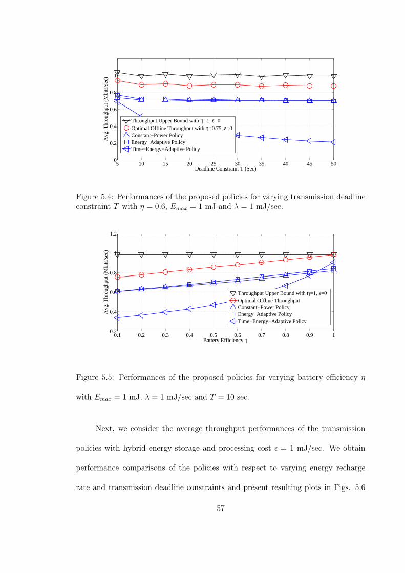
5 10 15 20 25 30 35 40 45 500

0.2

0.4

0.6

0.8

1

Deadline Constraint T (Sec)

Avg

. Thr

ough

put (

Mbi

ts/s

ec)

Throughput Upper Bound with η=1, ε=0Optimal Offline Throughput with η=0.75, ε=0Constant−Power PolicyEnergy−Adaptive PolicyTime−Energy−Adaptive Policy

Figure 5.4: Performances of the proposed policies for varying transmission deadlineconstraint T with η = 0.6, Emax = 1 mJ and λ = 1 mJ/sec.

0.1 0.2 0.3 0.4 0.5 0.6 0.7 0.8 0.9 10.2

0.4

0.6

0.8

1

1.2

Battery Efficiency η

Avg

. Thr

ough

put (

Mbi

ts/s

ec)

Throughput Upper Bound with η=1, ε=0Optimal Offline ThroughputConstant−Power PolicyEnergy−Adaptive PolicyTime−Energy−Adaptive Policy

Figure 5.5: Performances of the proposed policies for varying battery efficiency η

with Emax = 1 mJ, λ = 1 mJ/sec and T = 10 sec.

Next, we consider the average throughput performances of the transmission

policies with hybrid energy storage and processing cost ǫ = 1 mJ/sec. We obtain

performance comparisons of the policies with respect to varying energy recharge

rate and transmission deadline constraints and present resulting plots in Figs. 5.6

57

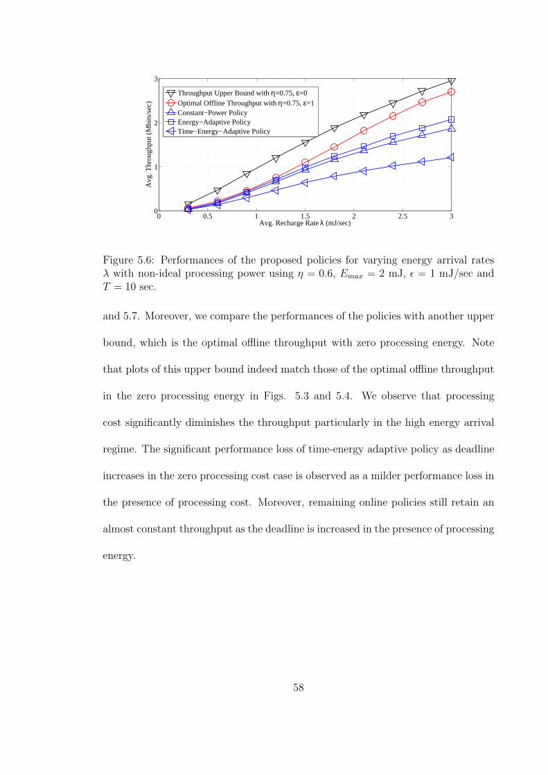
0 0.5 1 1.5 2 2.5 30

1

2

3

Avg. Recharge Rate λ (mJ/sec)

Avg

. Thr

ough

put (

Mbi

ts/s

ec)

Throughput Upper Bound with η=0.75, ε=0Optimal Offline Throughput with η=0.75, ε=1Constant−Power PolicyEnergy−Adaptive PolicyTime−Energy−Adaptive Policy

Figure 5.6: Performances of the proposed policies for varying energy arrival ratesλ with non-ideal processing power using η = 0.6, Emax = 2 mJ, ǫ = 1 mJ/sec andT = 10 sec.

and 5.7. Moreover, we compare the performances of the policies with another upper

bound, which is the optimal offline throughput with zero processing energy. Note

that plots of this upper bound indeed match those of the optimal offline throughput

in the zero processing energy in Figs. 5.3 and 5.4. We observe that processing

cost significantly diminishes the throughput particularly in the high energy arrival

regime. The significant performance loss of time-energy adaptive policy as deadline

increases in the zero processing cost case is observed as a milder performance loss in

the presence of processing cost. Moreover, remaining online policies still retain an

almost constant throughput as the deadline is increased in the presence of processing

energy.

58

5 10 15 20 25 30 35 40 45 500

0.2

0.4

0.6

0.8

1

Deadline Constraint T (Sec)

Avg

. Thr

ough

put (

Mbi

ts/s

ec)

Throughput Upper Bound with η=0.75, ε=0Optimal Offline Throughput with η=0.75, ε=1Constant−Power PolicyEnergy−Adaptive PolicyTime−Energy−Adaptive Policy

Figure 5.7: Performances of proposed policies for varying deadline constraint T with

non-ideal processing power using η = 0.6, Emax = 1 mJ, ǫ = 1 mJ/sec and λ = 1

mJ/sec.

59

Chapter 6

Conclusions

In this thesis, we consider optimal transmission schemes for energy harvesting

transmitters in wireless communication. The transmitter is equipped with a hybrid

energy storage unit, using a combination of a super-capacitor (SC) and a battery.

We first solve the optimization problem of maximizing the system throughput

in an AWGN channel under causality and storage capacity constraints, as imposed

by the energy harvesting profile. We analyze internal energy dynamics and their ad-

justment in the hybrid energy storage. Since the SC suffers from a storage capacity

limitation while battery has a low power density, the combination of both these ele-

ments offers better performance from a practical point of view. Although the energy

variables in both storage elements are highly coupled in this situation, we show that

the optimal solution is found by repeated application of the directional water-filling

algorithm. We generalize the single stage energy storage scenario and observe how

energy is spread in time subject to the aforementioned energy constraints.

Next, we extend the hybrid energy storage setup to include the processing

power consumed by the system circuitry. The processing power is assumed to be

constant and independent of the transmit power level. We observe that in presence

of a constant processing cost, the optimal transmission scheme is bursty in nature

and the directional water-filling algorithm gets transformed into a directional glue-

60

pouring algorithm. The bursty nature of communication is to transmit for a certain

fraction of the available time and for the rest of the time, the transmitter remains

inactive. Finally, we present numerical illustrations of the optimal policies and

performance comparisons with heuristic online transmission policies.

61

Bibliography

[1] A. Ephremides. Energy concerns in wireless networks. IEEE Wireless Commu-

nications, 9(4):48–59, Aug. 2002.

[2] V. Raghunathan, A. Kansal, J. Hsu, J. K. Friedman, and M. B. Srivastava.

Design considerations for solar energy harvesting wireless embedded systems.

In Int. Symp. on Inf. Process. in Sens. Nets, pages 457–462, April 2005.

[3] S. Sudevalayam and P. Kulkarni. Energy harvesting sensor nodes: Survey and

implications. IEEE Communication Surveys & Tutorials, 13(3):443–461, 2011.

[4] J. A. Stankovic and T. He. Energy management in sensor networks. Phil.

Trans. R. Soc., 370(1958):52–67, Nov. 2011.

[5] D. Niyato, E. Hossain, M. M. Rashid, and V. K. Bhargava. Wireless sensor

networks with energy harvesting technologies: A game-theoretic approach to

optimal energy management. IEEE Wireless Communications, 14(4):90–96,

Aug. 2007.

[6] N. Kumar and S. S. Manjunath. A reliable ultracapacitor based solar en-

ergy harvesting system for wireless sensor network enabled intelligent buildings.

IEEE-IAMA, pages 20–25, Sep.7-9 2011.

[7] A. S. Weddell, G. V. Merrett, T. J. Kazmierski, and B. A. Al-Hashimi. Accurate

supercapacitor modeling for energy-harvesting wireless sensor nodes. IEEE

Transactions on Circuits and Systems II, 58(12):911–915, Dec. 2011.

[8] G. V. Merrett and A. S. Weddell. Supercapacitor leakage in energy-harvesting

sensor nodes: Fact or fiction? Ninth International Conference on Networked

Sensing Systems (INSS), pages 1–5, Jun. 11-14 2012.

62

[9] C. Alippi and C. Galperti. Energy storage mechanisms in low power embedded

systems: Twin batteries and supercapacitors. Wireless VITAE, pages 31–35,

May.17-20 2009.

[10] J. Cao and A. Emadi. A new battery/ultracapacitor hybrid energy storage sys-

tem for electric, hybrid and plug-in hybrid electric vehicles. IEEE Transactions

on Power Electronics, 27(1):122–132, Jan. 2012.

[11] S. Saggini, F. Ongaro, C. Galperti, and P. Mattavelli. Supercapacitor-based

hybrid storage systems for energy harvesting in wireless sensor networks. IEEE-

APEC, pages 2281–2287, Feb. 21-25 2010.

[12] J. Yang and S. Ulukus. Optimal packet scheduling in an energy harvesting

communication system. IEEE Trans. Comm., 60(1):220–230, January 2012.

[13] K. Tutuncuoglu and A. Yener. Optimum transmission policies for battery lim-

ited energy harvesting nodes. IEEE Trans. Wireless Comm., 11(3):1180–1189,

March 2012.

[14] O. Ozel, K. Tutuncuoglu, J. Yang, S. Ulukus, and A. Yener. Transmission with

energy harvesting nodes in fading wireless channels: Optimal policies. IEEE

Jour. on Selected Areas in Commun., 29(8):1732–1743, September 2011.

[15] J. Yang, O. Ozel, and S. Ulukus. Broadcasting with an energy harvesting

rechargeable transmitter. IEEE Trans. Wireless Comm., 11(2):571–583, Febru-

ary 2012.

[16] O. Ozel, J. Yang, and S. Ulukus. Optimal broadcast scheduling for an energy

harvesting rechargeable transmitter with a finite capacity battery. IEEE Trans.

Wireless Comm., 11(6):2193–2203, June 2012.

63

[17] M. A. Antepli, E. Uysal-Biyikoglu, and H. Erkal. Optimal packet schedul-

ing on an energy harvesting broadcast link. IEEE Jour. on Selected Areas in

Commun., 29(8):1721–1731, September 2011.

[18] J. Yang and S. Ulukus. Optimal packet scheduling in a multiple access channel

with energy harvesting transmitters. Jour. of Comm. and Netw., 14(2):140–150,

April 2012.

[19] K. Tutuncuoglu and A. Yener. Sum-rate optimal power policies for energy

harvesting transmitters in an interference channel. Jour. of Comm. and Netw.,

14(2):151–161, April 2012.

[20] C. Huang, R. Zhang, and S. Cui. Throughput maximization for the Gaussian

relay channel with energy harvesting constraints. IEEE Jour. on Selected Areas

in Commun., 31(8):1469 – 1479, Aug. 2013.

[21] D. Gunduz and B. Devillers. Two-hop communication with energy harvesting.

In IEEE CAMSAP, December 2011.

[22] B. Devillers and D. Gunduz. A general framework for the optimization of

energy harvesting communication systems with battery imperfections. Jour. of

Comm. and Netw., 14(2):130 – 139, Apr. 2012.

[23] B. Gurakan, O. Ozel, J. Yang, and S. Ulukus. Energy cooperation in energy

harvesting wireless communications. In IEEE ISIT, July 2012.

[24] B. Gurakan, O. Ozel, J. Yang, and S. Ulukus. Two-way and multiple access

energy harvesting systems with energy cooperation. In Asilomar Conference,

November 2012.

[25] B. Gurakan, O. Ozel, J. Yang, and S. Ulukus. Energy cooperation in energy

harvesting two-way communications. In IEEE ICC, June 2013.

64

[26] J. Xu and R. Zhang. Throughput optimal policies for energy harvesting wireless

transmitters with non-ideal circuit power. 2012. Available at [ArXiv:1204.3818].

[27] O. Orhan, D. Gunduz, and E. Erkip. Throughput maximization for an energy

harvesting system with processing cost. In IEEE ITW, September 2012.

[28] K. Tutuncuoglu and A. Yener. Communicating using an energy harvesting

transmitter: Optimum policies under energy storage losses. IEEE Trans. Wire-

less Comm., submitted August 2012. Available at [arXiv:1208.6273].

[29] S. Luo, R. Zhang, and T. J. Lim. Optimal save-then-transmit protocol for

energy harvesting wireless transmitters. IEEE Transactions on Wireless Com-

munications, 12(3):1196–1207, Mar. 2013.

[30] X. Jiang, J. Polastre, and D. Culler. Perpetual environmentally powered sensor

networks. In Fourth Int. Symp. on Inf. Processing in Sens. Nets, April 2005.

[31] S. Cui, A. J. Goldsmith, and A. Bahai. Energy-constrained modulation opti-

mization. IEEE Trans. Wireless Commun., 4(5):2349–2360, September 2005.

[32] Q. Bai and J. A. Nossek. Throughput maximization for energy harvesting nodes

with generalized circuit power modelling. IEEE 13th International Workshop

on Signal Processing Advances in Wireless Communication, pages 485–489,

June 2012.

[33] M. Gregori and M. Payaro. Throughput maximization for a wireless energy

harvesting node considering the circuitry power consumption. IEEE Vehicular

Technology Conference, pages 1–5, September 2012.

[34] S. Boyd and L. Vandenberghe. Convex Optimization. Cambridge University

Press, United Kingdom, 2004.

65

[35] P. Youssef-Massaad, L. Zheng, and M. Medard. Bursty transmission and glue

pouring: On wireless channels with overhead costs. IEEE Trans. Wireless

Commun., 7(12):5188–5194, December 2008.

[36] M. Gorlatova, A. Wallwater, and G. Zussman. Networking low-power energy

harvesting devices: Measurements and algorithms. Proc. IEEE INFOCOM,

pages 1602–1610, April 2011.

66