ABSTRACT

Title of dissertation: SYNCHRONIZATION OF NETWORKCOUPLED CHAOTIC AND OSCILLATORYDYNAMICAL SYSTEMS

Gilad Barlev, Doctor of Philosophy, 2013

Dissertation directed by: Professor Edward OttDepartment of Physics

We consider various problems relating to synchronization in networks of cou-

pled oscillators. In Chapter 2 we extend a recent exact solution technique developed

for all-to-all connected Kuramoto oscillators to certain types of networks by con-

sidering large ensembles of system realizations. For certain network types, this

description allows for a reduction to a low dimensional system of equations. In

Chapter 3 we compute the Lyapunov spectrum of the Kuramoto model and con-

trast our results both with the results of other papers which studied similar systems

and with those we would expect to arise from a low dimensional description of the

macroscopic system state, demonstrating that the microscopic dynamics arise from

single oscillators interacting with the mean field. Finally, Chapter 4 considers an

adaptive coupling scheme for chaotic oscillators and explores under which conditions

the scheme is stable, as well as the quality of the stability.

SYNCHRONIZATION OF NETWORK COUPLED CHAOTICAND OSCILLATORY DYNAMICAL SYSTEMS

by

Gilad Barlev

Dissertation submitted to the Faculty of the Graduate School of theUniversity of Maryland, College Park in partial fulfillment

of the requirements for the degree ofDoctor of Philosophy

2013

Advisory Committee:Professor Edward Ott, Chair/AdvisorProfessor Rajarshi RoyProfessor Michelle GirvanProfessor Thomas AntonsenProfessor Thomas Murphy

c© Copyright byGilad Barlev

2013

Dedication

For Jen, who reminds me why I do this work, who puts it in perspective, and

who gives me something to look forward to at the end of each day.

ii

Acknowledgments

I thank my co-authors and collaborators, Prof. Francesco Sorrentino, Prof.

Thomas Antonsen and especially my advisor, Dr. Edward Ott.

This work was supported by grants from the U.S. Office of Naval Research

(N00014-07-1-0734) and the U.S. Army Research Office (W911NF-12-1-1010).

iii

Table of Contents

List of Figures vi

1 Introduction 11.1 The Kuramoto Model and Order . . . . . . . . . . . . . . . . . . . . 11.2 Lyapunov Exponents and Stability . . . . . . . . . . . . . . . . . . . 31.3 Outline . . . . . . . . . . . . . . . . . . . . . . . . . . . . . . . . . . . 5

2 The Dynamics of Network Coupled Phase Oscillators: An Ensemble Ap-proach 72.1 Overview . . . . . . . . . . . . . . . . . . . . . . . . . . . . . . . . . . 72.2 Introduction . . . . . . . . . . . . . . . . . . . . . . . . . . . . . . . . 8

2.2.1 Background . . . . . . . . . . . . . . . . . . . . . . . . . . . . 82.2.2 Numerical Methods . . . . . . . . . . . . . . . . . . . . . . . . 11

2.3 Unimodal Frequency Distribution . . . . . . . . . . . . . . . . . . . . 132.3.1 Formulation . . . . . . . . . . . . . . . . . . . . . . . . . . . . 132.3.2 Bulk Order Parameter . . . . . . . . . . . . . . . . . . . . . . 202.3.3 Steady State . . . . . . . . . . . . . . . . . . . . . . . . . . . . 212.3.4 Maximum Eigenvalue Approximation . . . . . . . . . . . . . . 242.3.5 Special case: Uniform in-degree . . . . . . . . . . . . . . . . . 29

2.4 Bimodal Frequency Distribution . . . . . . . . . . . . . . . . . . . . . 322.4.1 Formulation . . . . . . . . . . . . . . . . . . . . . . . . . . . . 322.4.2 Uniform In-degree . . . . . . . . . . . . . . . . . . . . . . . . . 332.4.3 Dynamics . . . . . . . . . . . . . . . . . . . . . . . . . . . . . 35

2.5 Conclusion . . . . . . . . . . . . . . . . . . . . . . . . . . . . . . . . . 44

3 Lyapunov Spectrum of the Kuramoto Model 483.1 Overview . . . . . . . . . . . . . . . . . . . . . . . . . . . . . . . . . . 483.2 Introduction . . . . . . . . . . . . . . . . . . . . . . . . . . . . . . . . 483.3 Macroscopic Description . . . . . . . . . . . . . . . . . . . . . . . . . 503.4 Microscopic Lyapunov Spectrum . . . . . . . . . . . . . . . . . . . . . 52

3.4.1 Average Lyapunov Spectrum . . . . . . . . . . . . . . . . . . . 543.4.2 Near-Zero Exponents . . . . . . . . . . . . . . . . . . . . . . . 57

iv

3.4.3 Comparison with Macroscopic Dynamics . . . . . . . . . . . . 603.5 Single Oscillator Approximation of Lyapunov Vectors and Exponents

Based on the Behavior in the Mean Field . . . . . . . . . . . . . . . . 633.6 Conclusion . . . . . . . . . . . . . . . . . . . . . . . . . . . . . . . . . 69

4 The Stability of Adaptive Synchronizationof Chaotic Systems 714.1 Overview . . . . . . . . . . . . . . . . . . . . . . . . . . . . . . . . . . 714.2 Introduction . . . . . . . . . . . . . . . . . . . . . . . . . . . . . . . . 724.3 Adaptive strategy formulation . . . . . . . . . . . . . . . . . . . . . . 744.4 Stability analysis . . . . . . . . . . . . . . . . . . . . . . . . . . . . . 77

4.4.1 Linearization and master stability function . . . . . . . . . . . 774.4.2 Generalized adaptive strategy . . . . . . . . . . . . . . . . . . 82

4.5 Numerical experiments . . . . . . . . . . . . . . . . . . . . . . . . . . 844.6 Conclusion . . . . . . . . . . . . . . . . . . . . . . . . . . . . . . . . . 91

A Stability of the generalized adaptive strategy 97

B Determination of unstable periodic orbits 98

Bibliography 100

v

List of Figures

1.1 The Kuramoto model is often visualized as beads on a ring, coupledby an attractive pseudo-force whose magnitude is proportional to thedistance between the oscillators. . . . . . . . . . . . . . . . . . . . . . 2

1.2 The order parameter R (Eq. (1.2)) can be visualized as the vectorfrom the center of the ring to the center of mass of the system. . . . . 3

1.3 Example of Lyapunov dynamics. As a cloud of states around someinitial condition are evolved, that cloud will expand in some directionsand contract in others. The rates of expansion and contraction alongdifferent orthogonal axes give the Lyapunov exponents of the system. 4

2.1 In-degree distributions for the the Erdos-Renyi and scale-free net-works used in this chapter. The Erdos-Renyi network’s degree dis-tribution (dot-dashed line) is peaked around 100. Past a minimumdegree, the scale-free network takes on a degree distribution (dottedline) of the form P (d) ∼ d−2.5, as is more clearly seen in the inset,which is the same plot shown on a log-log scale. . . . . . . . . . . . . 14

2.2 Eigenspectrum plots for the the three networks used in this chap-ter: (a) a directed network with uniform in-degree, (b) an undi-rected Erdos-Renyi network and (c) an undirected scale-free network(γ = 2.5). In all cases, N = 104 and λ1 ' 100. Since the Erdos-Renyiand scale-free graphs are undirected, all eigenvalues in those cases arereal. . . . . . . . . . . . . . . . . . . . . . . . . . . . . . . . . . . . . 15

vi

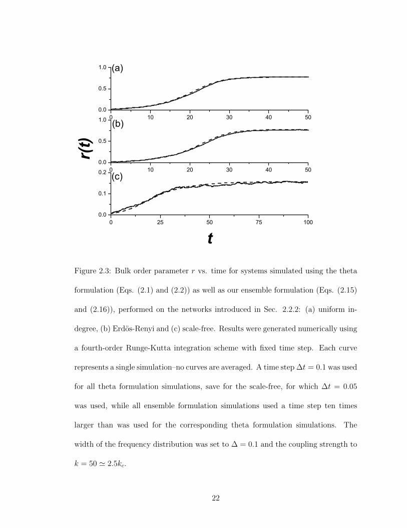
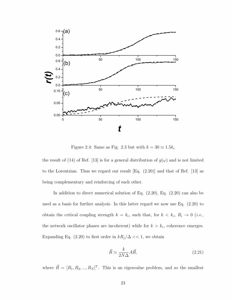
2.3 Bulk order parameter r vs. time for systems simulated using thetheta formulation (Eqs. (2.1) and (2.2)) as well as our ensembleformulation (Eqs. (2.15) and (2.16)), performed on the networksintroduced in Sec. 2.2.2: (a) uniform in-degree, (b) Erdos-Renyi and(c) scale-free. Results were generated numerically using a fourth-order Runge-Kutta integration scheme with fixed time step. Eachcurve represents a single simulation–no curves are averaged. A timestep ∆t = 0.1 was used for all theta formulation simulations, savefor the scale-free, for which ∆t = 0.05 was used, while all ensembleformulation simulations used a time step ten times larger than wasused for the corresponding theta formulation simulations. The widthof the frequency distribution was set to ∆ = 0.1 and the couplingstrength to k = 50 ' 2.5kc. . . . . . . . . . . . . . . . . . . . . . . . . 22

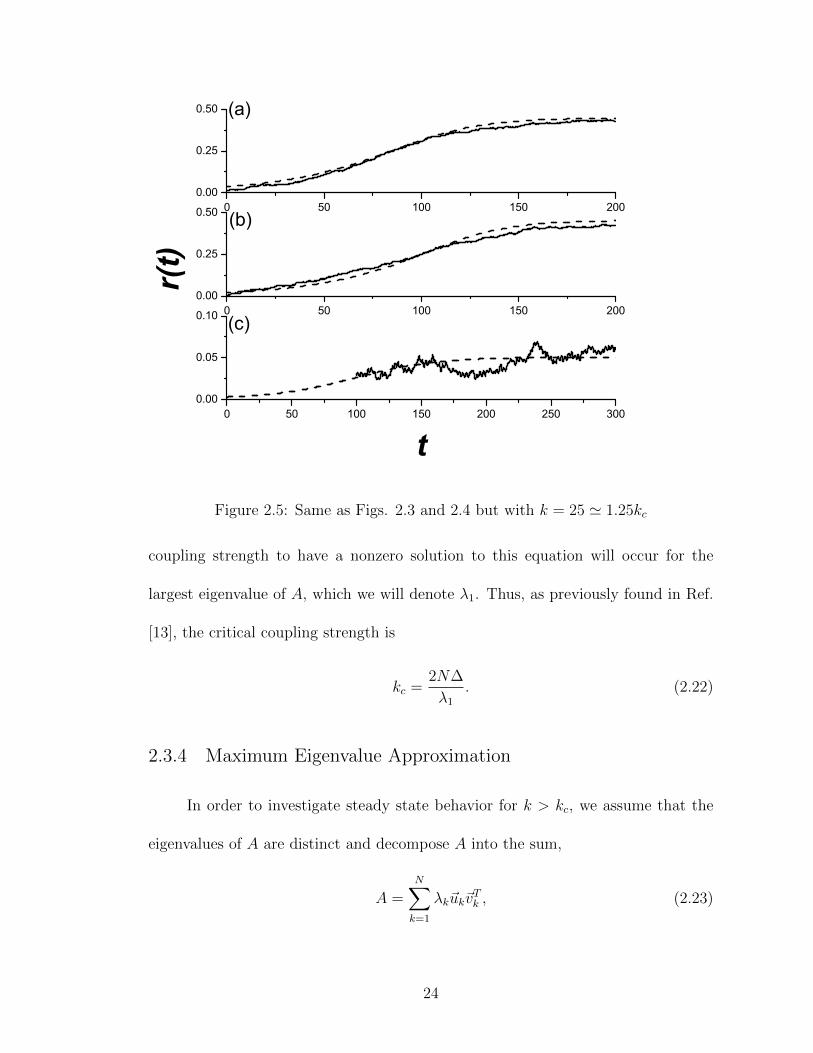
2.4 Same as Fig. 2.3 but with k = 30 ' 1.5kc . . . . . . . . . . . . . . . . 232.5 Same as Figs. 2.3 and 2.4 but with k = 25 ' 1.25kc . . . . . . . . . . 242.6 Long-time-averaged values of r vs. k for systems simulated using the

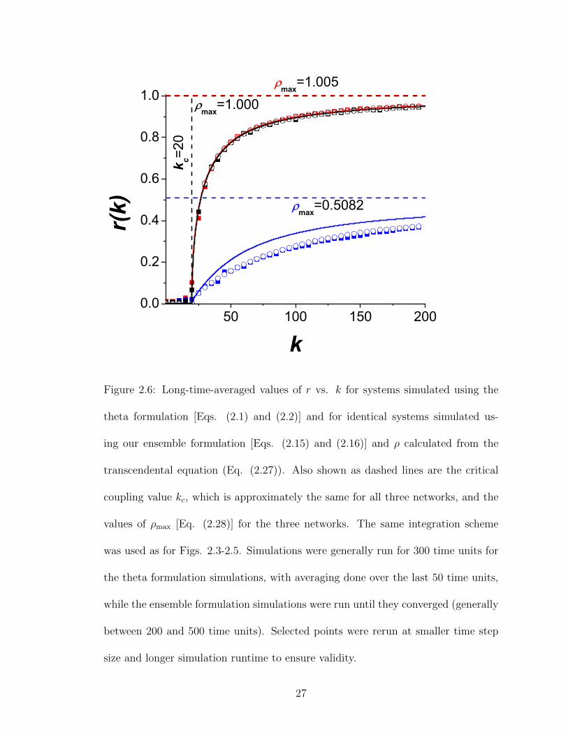
theta formulation [Eqs. (2.1) and (2.2)] and for identical systemssimulated using our ensemble formulation [Eqs. (2.15) and (2.16)]and ρ calculated from the transcendental equation (Eq. (2.27)). Alsoshown as dashed lines are the critical coupling value kc, which isapproximately the same for all three networks, and the values of ρmax

[Eq. (2.28)] for the three networks. The same integration scheme wasused as for Figs. 2.3-2.5. Simulations were generally run for 300 timeunits for the theta formulation simulations, with averaging done overthe last 50 time units, while the ensemble formulation simulationswere run until they converged (generally between 200 and 500 timeunits). Selected points were rerun at smaller time step size and longersimulation runtime to ensure validity. . . . . . . . . . . . . . . . . . . 27

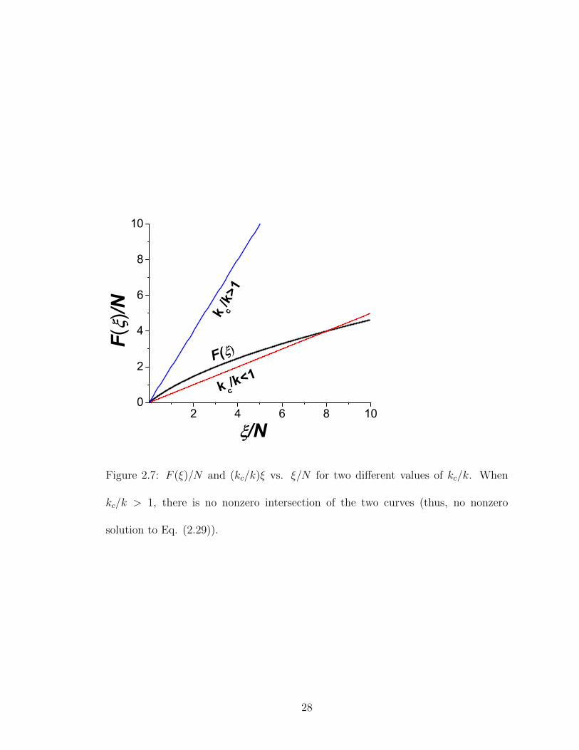
2.7 F (ξ)/N and (kc/k)ξ vs. ξ/N for two different values of kc/k. Whenkc/k > 1, there is no nonzero intersection of the two curves (thus, nononzero solution to Eq. (2.29)). . . . . . . . . . . . . . . . . . . . . . 28

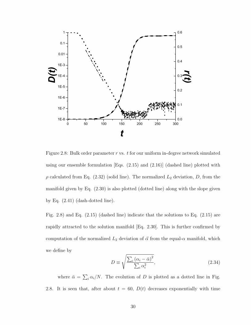
2.8 Bulk order parameter r vs. t for our uniform in-degree network simu-lated using our ensemble formulation [Eqs. (2.15) and (2.16)] (dashedline) plotted with ρ calculated from Eq. (2.32) (solid line). The nor-malized L2 deviation, D, from the manifold given by Eq. (2.30) isalso plotted (dotted line) along with the slope given by Eq. (2.41)(dash-dotted line). . . . . . . . . . . . . . . . . . . . . . . . . . . . . 30

2.9 (a) Bulk order parameter r plotted vs. time for a theta formulationsimulations [Eq. (2.1)] on our uniform in-degree network using a bi-modal distribution (solid line) and for a simulation using Eqs. (2.51)and (2.52) (dashed line). A time step of 0.05 was used for both simu-lations. The parameters of the simulation were k = 40, ∆ = 0.5 andω0 = 0.2. (b) A parametric polar plot (a, ψ) of the same simulations,starting at incoherent initial conditions (r << 1). . . . . . . . . . . . 36

vii

2.10 Phase diagram in (ω0, ∆) parameter space showing regions corre-sponding to different attractor types denoted by I (incoherent steadystate attractor at r = 0), SS (steady state attractor with r > 0), andLC (limit cycle attractor corresponding to time periodic variation ofr). Bifurcations of these attractors occur as the region boundaries arecrossed [39]. The dashed horizontal lines at ∆ = 1.5, 1.1, 0.9 and 0.5correspond to the scans of parameter ω0 shown in Fig. 2.11. . . . . . 38

2.11 Long-time behavior of r vs. ω0 for systems simulated using the thetaformulation [Eqs. (2.1) and (2.2)], plotted in black, and our ensem-ble formulation [Eqs. (2.51) and (2.52)], plotted in green, for fourdifferent values of ∆: (a) ∆ = 1.5, (b) ∆ = 1.1, (c) ∆ = 0.9 and (d)∆ = 0.5. We discard the first 1, 000 time units of our simulations,time average the results over the next 1, 000 time units [40] and plotthe averages as solid squares. When the trajectories are apparentlylimit cycles, the results are plotted as vertical bars indicating therange of r values in the oscillation. Vertical dashed lines representthe region boundaries of Fig. 2.10. The coupling strength k washeld fixed at k = 40. Simulations were performed on the uniform in-degree network introduced in Sec. 2.2.2. Where needed, simulationsin this figure were run twice, once starting from an incoherent stateand again from a coherent initial condition (obtained by pre-runningthe simulations for large k). . . . . . . . . . . . . . . . . . . . . . . . 40

2.12 Polar plot of (a, ψ) for a variety of initial conditions for ∆ = 1.1 andω0 = 1.10. The solid lines represent simulations performed using ourreduced ensemble equations [Eqs. (2.51) and (2.52)] and are color-coded to indicate which attractor each simulation ended on (blue forsynchronized steady-state, red for incoherent). The locations of eachattractor and of a saddle point are marked by grey dots. The regionssurrounding each attractor are blown up in (b) (SS) and (c) (I), withorbits from theta formulation simulations [Eq. (2.1)] shown in blackwith transients removed. . . . . . . . . . . . . . . . . . . . . . . . . . 42

2.13 Polar plot of (a, ψ) for a variety of initial conditions for ∆ = 1.1 andω0 = 1.05. The solid lines represent simulations performed using ourreduced ensemble equations [Eqs. (2.51) and (2.52)] and are color-coded to indicate which attractor each simulation ended on (blue forsynchronized steady-state, red for incoherent). The location of eachattractor and of the saddle point is marked by a grey dot. (b) Amagnification of the region of interest, with points on the orbit ofa theta formulation simulation [Eq. (2.1)] plotted in black, showingthe system starting in the incoherent attractor and escaping to thesteady-state attractor. (c) a plotted vs. time for the same thetaformulation simulation plotted in (b). . . . . . . . . . . . . . . . . . . 43

2.14 Two of the graphs from Fig. 2.11 re-plotted to include simulationsdone on the Erdos-Renyi network (red) introduced in Sec. 2.2.2. . . . 45

viii

3.1 The magnitude ρ of the order parameter R vs. time t for a systemof N = 105 oscillators whose natural frequencies ωj were selectedfrom a Lorentzian distribution of width ∆ = 1 (so kc = 2) and centerΩ = 0. The coupling strength was set to k = 4 = 2kc. The systemwas initialized in a random (incoherent) state and was evolved ac-cording to Eq. (3.1). Insets show on a log-linear scale the distanceof the system from the two steady-state solutions: (a) the unstableincoherent state ρ = 0 and (b) the stable coherent state ρ = 1/

√2, as

calculated from Eq. (3.6). The slopes of the dashed lines correspondto the predicted Lyapunov exponents hIL and hSL. . . . . . . . . . . . 53

3.2 The Lyapunov spectrum plotted vs. coupling strength k for one real-ization of a system of N = 200 oscillators whose natural frequencieswere sampled randomly from a Lorentzian distribution with width∆ = 1. Black solid curves: the computed Lyapunov spectrum basedon the evolution of Eq. (3.1). Blue dashed curves: the Lyapunovspectrum as predicted using Eq. (3.19) of Sec. 3.5. Red dotted lines:the low dimensional spectrum, Eqs. (3.7), (3.9) and (3.10). Inset:Long-time values of the magnitude ρ of the order parameter R plot-ted vs. k. Black solid curve: average long-time value of ρ of thesystem as calculated using Eq. (3.3). Red dots: Eq. (3.6) as thesynchronized steady state solution to the low-dimensional equation,Eq. (3.4). . . . . . . . . . . . . . . . . . . . . . . . . . . . . . . . . . 55

3.3 Histograms of the average Lyapunov spectra for approximately 2500realizations of our system (different values of ωj each time). Separatecurves are plotted for four values of the coupling strength k: k = 1(black), which is below kc, k = 2 = kc (red), k = 4 (green), which istwice kc, and k = 10 (blue), which is much larger than kc. Histogramsfor the expected Lyapunov exponents according to the single oscillatorhypothesis of Sec. 3.5 are plotted in faded colors. The vertical dashedlines indicate the locations of the low-dimensional Lyapunov exponenthSL (Eq. (3.10)) for each curve, k > kc, while the vertical dotted linesindicate the locations of the asymptotic value h∞ (Eq. (3.21)). . . . . 56

3.4 Figure 3.3 enlarged around h = 0 using a smaller bin size. . . . . . . . 573.5 Median values of h1 plotted vs. number of oscillators N for an

ensemble of realizations, at three values of coupling strength: (a)k = 1 < kc, (b) k = 2 = kc and (c) k = 4 > kc. Positive errorbars correspond to the range between the second and third quartiles,negative error bars to between the first and second. . . . . . . . . . . 58

3.6 Fraction of positive Lyapunov exponents, h > 0, for large ensemblesof realizations of our system for various values of N at four values ofcoupling strength k. . . . . . . . . . . . . . . . . . . . . . . . . . . . . 59

ix

3.7 Scatterplot showing the macroscopicness of each Lyapunov vector, ascomputed from Eq. (3.14), vs. each vector’s associated Lyapunovnumber hi for a single realization of a system of N = 500 oscillatorswith coupling strength k = 4. The dashed red line correspond to thelow dimensional Lyapunov exponent hSL. . . . . . . . . . . . . . . . . 62

3.8 (a) Grayscale heat map showing the magnitudes of the inner products(darker color indicates greater magnitude) of each of the N + 1 pre-dicted Lyapunov vectors—~v0 corresponding to Eq. (3.12) and ~vSOH1 -~vSOHN corresponding to Eq. (3.18)—with the N Lyapunov vectors ofour system of N = 200 oscillators for a coupling strength of k = 4.Each set of vectors was ranked by their corresponding Lyapunov ex-ponent, hn > hn+1. (b) Same as (a) but for k = 10. (c) The valuesof the Lyapunov exponents associated with each of the Lyapunovvectors of the system for (a) and (b). In both cases, V (0), the ini-tial matrix for our algorithm, was generated by selecting Vmn(0)randomly and uniformly from the range [−1, 1], and the calculationruntime was 500 time units. . . . . . . . . . . . . . . . . . . . . . . . 64

3.9 Same as Fig. 3.3 but for approximately 1000 realizations of a systemof 500 oscillators. . . . . . . . . . . . . . . . . . . . . . . . . . . . . . 67

3.10 The Lyapunov spectrum for a system of N = 200 oscillators withnatural frequencies sampled randomly from a Gaussian distributionwith width σ = 1 plotted vs. coupling strength k. Black solid: thehigh dimensional spectrum based on the evolution of Eq. (3.1). Bluedashed: the high dimensional spectrum as predicted using the singleoscillator hypothesis Eq. (3.19). Inset: Long-time average values ofρ as calculated using Eq. (3.3), plotted vs. k. . . . . . . . . . . . . . 68

4.1 The plot shows the master stability function M(ξ) versus ξ for thecase in which no adaptation was introduced, corresponding to σ ≡ 1(black continuous line) and for three different values of ν, i.e., ν =0.1, 2, 6 (dashed and dotted lines). The master stability functions ob-tained by choosing xs(t) to be a typical chaotic orbit in the attractor(respectively, the maximally unstable periodic orbit embedded in theattractor of period up to four) are in black (respectively, grey). F (x)is the Rossler equation (4.18), H(x(t)) = u(t), and Γ = [1, 0, 0]T . . . 85

4.2 The figure is a level curve plot in ξ-ν space of the values assumed bythe master stability function M , evaluated for xs(t) being a typicalchaotic orbit. The area of stability (corresponding to M < 0) is de-limited by the thick 0-level contour line. F (x) is the Rossler equation(4.18), H(x(t)) = u(t), and Γ = [1, 0, 0]T . . . . . . . . . . . . . . . . 88

x

4.3 In plot (a), thick solid curves (thick dashed curves) bound the areain which the master stability function M(ξ, ν) is negative for xs(t)corresponding to a typical chaotic orbit in the Rossler attractor (forxs(t) corresponding to the maximally unstable periodic orbit embed-ded in the attractor of period up to four), F (x) is the Rossler equation(4.18), H(x(t)) = u(t), and Γ = [1, 0, 0]T . Each data point shown inthe figure is the result of a simulation involving a sender (maestro)system connected to a receiver, where the receiver state was initial-ized by a displacement of 10−8 from the sender state. A step-size of10−4 was used for a run time of 105 time units. If, in that time span,the synchronization error E never converged to 0 and, at some point,exceeded 0.1, the run was considered to be unstable (× symbols). IfE converged to 0, a 1% mismatch in the Rossler parameter a wasintroduced to the receiver, and the run was repeated with an initialseparation of 0. Then, if E ever exceeded 0.1, the run was consideredto be bubbling (green circles), otherwise the run was considered to bestable (red triangles). Plot (b) is a blow up of the lower left corner ofplot (a). Plot (c) shows the synchronizability ratios st (solid curve)and sp (dashed curve) versus ν. The missing data for the dashed curveare a result of the low period orbits not having a range of stability forthose values of ν. The synchronizability ratios for the nonadaptivecase were found to be equal to those in the limit ν → 0. . . . . . . . 93

4.4 The figure shows the synchronization error E(t) versus t for a simplenetwork consisting of a sender connected to a receiver (Eqs. (4.21)),F (x) is the Rossler equation (4.18), H(x(t)) = u(t), Γ = [1, 0, 0]T ,γ = 5, ν = 2.5, A(t) = 1, dt = 10−3. The receiver has a 0.1%mismatch in the parameter a. The two insets are zooms showingphase-space projections in the plane (u2, v2), over two different timeintervals. Inset (b) corresponds to a typical chaotic orbit for whichthe synchronization error is small, i.e., E(t) < 5 × 10−2, while inset(a) corresponds to an unstable period 4 periodic orbit embedded inthe attractor, for which E(t) is eventually large (i.e., a burst occurs). 94

4.5 The plot shows the area in the parameter space (φ, ξ) in whichM(ξ, φ)obtained from (4.16) is negative, for three different values of ν =[0.1, 2.0, 6.0]; F (x) is the Rossler equation (4.18), H(x(t)) = u(t),and Γ = [1, 0, 0]T . The stability areas are upper and lower boundedby the ξ+ curve and the ξ− curve, plotted as function of φ. As thefigure shows, at φ = 2, ξ+ and ξ− are independent of ν, correspondingto the case of no-adaptation. . . . . . . . . . . . . . . . . . . . . . . 95

4.6 The figure is a plot of the synchronization error E(t) (defined inEq. (4.22)) versus t for a simple network consisting of a senderconnected to a receiver (Eqs. (4.21)), F (x) is the Rossler equa-tion (4.18), H(x(t)) = u(t), Γ = [1, 0, 0]T , ν = 1, γ = 2, A(t) =1 + 0.2 sin(2π × 10−3t), dt = 10−3. As can be seen, the dynamics ofE(t) exhibits intermittent bursting. . . . . . . . . . . . . . . . . . . . 96

xi

Chapter 1: Introduction

Synchronization is an important behavior in systems of coupled units. Some-

times, as in communications, it is desirable for multiple units to behave in a coor-

dinated fashion. In other circumstances, such collective behavior in large systems

can be disastrous, as in epileptic seizures. The Kuramoto model is perhaps the

simplest system used to study synchronization in large populations, and it is the

focus of Chapters 2 and 3. Chapter 4 analyzes the stability of an adaptive method

for synchronizing chaotic oscillators. This is done through use of a Master Stability

Function which relies on Lyapunov analysis, which is also used to characterize the

microscopic behavior of the Kuramoto model in Chapter 3.

1.1 The Kuramoto Model and Order

The Kuramoto model is a simple phase oscillator model in which each oscillator

i in a system of N oscillators is represented by a phase angle θi, with dynamics given

by

dθj(t)

dt= ωj +

k

N

N∑j=1

sin (θj(t)− θi(t)) , (1.1)

with each oscillator having its own so-called “natural frequency” ωi which gives the

rate at which the oscillator evolves in the absence of coupling (k = 0). This system

1

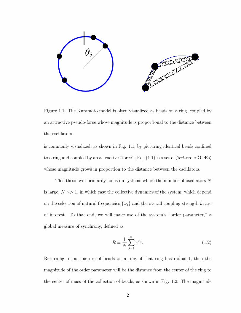
Figure 1.1: The Kuramoto model is often visualized as beads on a ring, coupled by

an attractive pseudo-force whose magnitude is proportional to the distance between

the oscillators.

is commonly visualized, as shown in Fig. 1.1, by picturing identical beads confined

to a ring and coupled by an attractive “force” (Eq. (1.1) is a set of first-order ODEs)

whose magnitude grows in proportion to the distance between the oscillators.

This thesis will primarily focus on systems where the number of oscillators N

is large, N >> 1, in which case the collective dynamics of the system, which depend

on the selection of natural frequencies ωj and the overall coupling strength k, are

of interest. To that end, we will make use of the system’s “order parameter,” a

global measure of synchrony, defined as

R ≡ 1

N

N∑j=1

eiθj . (1.2)

Returning to our picture of beads on a ring, if that ring has radius 1, then the

magnitude of the order parameter will be the distance from the center of the ring to

the center of mass of the collection of beads, as shown in Fig. 1.2. The magnitude

2

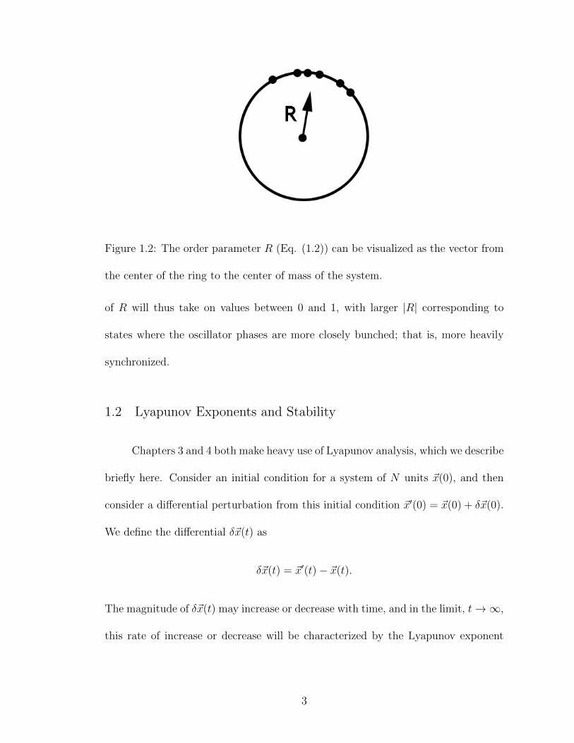
Figure 1.2: The order parameter R (Eq. (1.2)) can be visualized as the vector from

the center of the ring to the center of mass of the system.

of R will thus take on values between 0 and 1, with larger |R| corresponding to

states where the oscillator phases are more closely bunched; that is, more heavily

synchronized.

1.2 Lyapunov Exponents and Stability

Chapters 3 and 4 both make heavy use of Lyapunov analysis, which we describe

briefly here. Consider an initial condition for a system of N units ~x(0), and then

consider a differential perturbation from this initial condition ~x′(0) = ~x(0) + δ~x(0).

We define the differential δ~x(t) as

δ~x(t) = ~x′(t)− ~x(t).

The magnitude of δ~x(t) may increase or decrease with time, and in the limit, t→∞,

this rate of increase or decrease will be characterized by the Lyapunov exponent

3

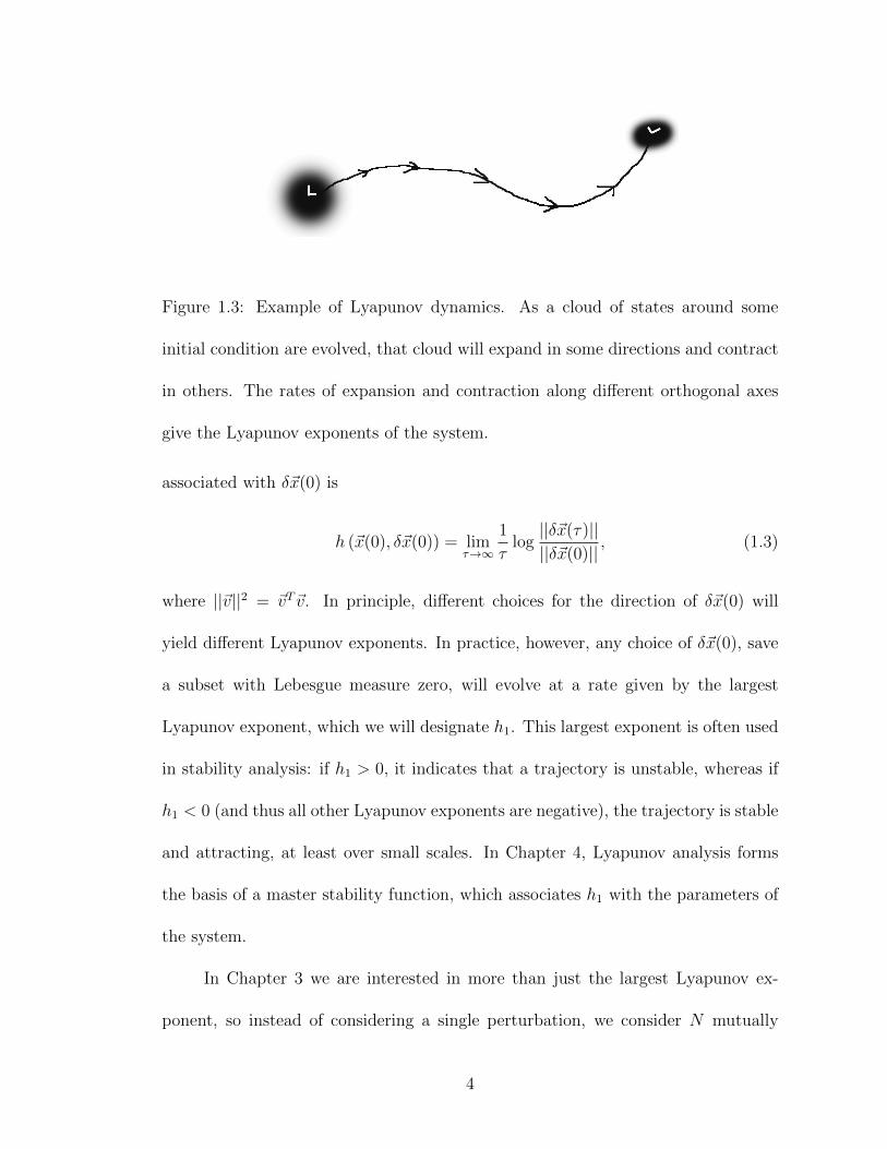
Figure 1.3: Example of Lyapunov dynamics. As a cloud of states around some

initial condition are evolved, that cloud will expand in some directions and contract

in others. The rates of expansion and contraction along different orthogonal axes

give the Lyapunov exponents of the system.

associated with δ~x(0) is

h (~x(0), δ~x(0)) = limτ→∞

1

τlog||δ~x(τ)||||δ~x(0)||

, (1.3)

where ||~v||2 = ~vT~v. In principle, different choices for the direction of δ~x(0) will

yield different Lyapunov exponents. In practice, however, any choice of δ~x(0), save

a subset with Lebesgue measure zero, will evolve at a rate given by the largest

Lyapunov exponent, which we will designate h1. This largest exponent is often used

in stability analysis: if h1 > 0, it indicates that a trajectory is unstable, whereas if

h1 < 0 (and thus all other Lyapunov exponents are negative), the trajectory is stable

and attracting, at least over small scales. In Chapter 4, Lyapunov analysis forms

the basis of a master stability function, which associates h1 with the parameters of

the system.

In Chapter 3 we are interested in more than just the largest Lyapunov ex-

ponent, so instead of considering a single perturbation, we consider N mutually

4

orthogonal tangent vectors ~vm which form a complete basis for the space. If ~vm

are chosen such that they evolve orthornormally, then perturbations in the direc-

tions of these tangent vectors will give a set of N Lyapunov exponents hm which

characterize the microscopic evolution of the system.

1.3 Outline

The problems addressed and main results are as follows.

Chapter 2: In this chapter we consider a variant of the Kuramoto problem

(Eq. (1.1)) in which the coupling between oscillators, rather than being all-to-all

and equal strength, is determined by a network. That is, the coupling term in Eq.

(1.1) is replaced by

k

N

N∑j=1

Aij sin (θj(t)− θi(t)) ,

where Aij = 1 if there is a network edge from j to i and Aij = 0 if not. The main

result is that for large N a recent exact solution technique for the all-to-all case can

be extended to obtain results for certain types of newtorks.

Chapter 3: In this chapter we compute the full N -dimensional Lyapunov spec-

trum for a system of Kuramoto oscillators and show that the majority of Lyapunov

exponents and their associated vectors are well-described as arising from the evo-

lution of single oscillators interacting with the mean field. We contrast our results

both with the results of other papers which studied similar systems and with those

we would expect to arise from a low dimensional description of the macroscopic

system state.

5

Chapter 4: In the final chapter we consider an adaptive coupling scheme for

nearly-identical chaotic oscillators and explore through numerical simulations the

conditions under which the scheme is stable. Using Master Stability analysis, we

differentiate between “high quality” synchronization, in which the oscillators re-

main synchronized through the entire attractor, and conditions where “bubbling”

(occasional bursts of desynchrony) occurs.

6

Chapter 2: The Dynamics of Network Coupled Phase Oscillators:

An Ensemble Approach

2.1 Overview

We consider the dynamics of many phase oscillators that interact through a

coupling network. For a given network connectivity we further consider an ensem-

ble of such systems where, for each ensemble member, the set of oscillator natural

frequencies is independently and randomly chosen according to a given distribution

function. We then seek a statistical description of the dynamics of this ensemble.

Use of this approach allows us to apply the recently developed ansatz of Ott and

Antonsen [Chaos 18, 037113 (2008)] to the marginal distribution of the ensemble of

states at each node. This, in turn, results in a reduced set of ordinary differential

equations determining these marginal distribution functions. The new set facilitates

the analysis of network dynamics in several ways: (i) the time evolution of the re-

duced system of ensemble equations is much smoother, and thus numerical solutions

can be obtained much faster by use of longer time steps; (ii) the new set of equa-

tions can be used as a basis for obtaining analytical results; and (iii) for a certain

type of network, a reduction to a low dimensional description of the entire network

7

dynamics is possible. We illustrate our approach with numerical experiments on a

network version of the classical Kuramoto problem, first with a unimodal frequency

distribution, and then with a bimodal distribution. In the latter case, the network

dynamics is characterized by bifurcations and hysteresis involving a variety of steady

and periodic attractors.

2.2 Introduction

2.2.1 Background

Dynamical processes on networks are a central theme in the study of large

complex systems. Issues in this general class of problems include disease spread,

communications, opinion formation and synchronization, among others [1, 2]. In

this chapter we will be concerned with synchronization of N >> 1 nonidentical

oscillatory dynamical systems that are coupled to each other via a network whose

adjacency matrix we denote A (Aij = 1 if there is a link from j to i and Aij = 0

if there is no link). Furthermore, we will assume that the state of each oscillator i

is completely described by its phase θi (0 ≤ θi < 2π). Such oscillators are called

“phase oscillators.”

For the examples treated in this chapter, the dynamics will be taken to be

described by

dθi(t)

dt= ωi +

k

N

N∑j=1

Aij sin(θj − θi). (2.1)

In the special case where Aij = 1 for all i and j, we recover the classical, glob-

ally coupled, all-to-all Kuramoto model [3–7]. We emphasize that, although our

8

examples in Secs. 2.3 and 2.4 are of the form specified in Eq. (2.1), the general

technique that our chapter will present is also applicable to other types of coupling

and other types of systems (see Refs. [7–9] for a discussion of various system types

and problems in the special context of global all-to-all coupling).

The case of network coupling (i.e., nontrivial A in Eq. (2.1)) has recieved much

recent attention (e.g. Refs. [10–14]), but general methods for facilitating analysis

and understanding of large network coupled systems of phase oscillators (either of

the type of Eq. (2.1) or more generally) have been lacking. In contrast, Refs. [8]

and [9] have recently provided a broadly applicable analytical technique for various

types of globally all-to-all coupled systems. This technique has so far been applied to

a diverse set of issues. These include modeling of birdsong [15], bursting neurons [16],

pedestrian induced shaking of London’s Millennium Bridge [17], circadian rhythm

[18], Josephson junction circuits [19], coupled excitable systems [20], noise [21],

bimodal distributions of oscillator frequencies [22, 23], interaction time delay [24],

phase resetting [25], time dependent connectivity [26], groups of coupled oscillators

[27] and chimera states [28–33] (i.e., states where one oscillator group is coherent

while another is incoherent).

The utility of Refs. [8] and [9] for treating all-to-all coupled systems of phase

oscillators suggests that an extension to network coupling, if possible, might prove

useful. This chapter addresses the goal of making such an extension, and we test

and illustrate our approach by application to the system of equations given by Eq.

(2.1).

In defining the system (Eq. ( 2.1)), most previous works assign the values of

9

the oscillator natural frequencies ωi by choosing them randomly and independently

from some prespecified distribution function. Behavior of the system with these

specified natural frequencies can then be investigated, e.g., by numerical solution of

Eq. (2.1). If one is interested in the statistics of the behavior originating from many

different random choices of the natural frequencies, one could, in principle, integrate

Eq. (2.1) with many such choices, and then examine the results. Here we consider

a procedure related to this. In particular, we imagine an ensemble of systems,

all with the same adjacency matrix A, but with each ensemble member having a

different randomly chosen collection ωi of natural frequencies, and we consider

the evolution of this entire ensemble. This evolution can be thought of as being

characterized by the set of marginal oscillator state distributions, fi(θi, ωi, t), giving

the probability density that oscillator i of a randomly selected ensemble member has

natural frequency ωi and, at time t, has the phase θi. At first sight, this appears to

be a much more demanding problem than Eq. (2.1), since the time t state of node

i of the ensemble is now described by a distribution function, while in Eq. (2.1) the

time t state of node i is described by the single scalar variable θi. However, by use of

the method of Refs. [8] and [9], we will show that, under appropriate conditions, the

ensemble problem can be reduced to a set of ordinary differential equations whose

size is similar to that of the original system; that is, for the case considered in Sec.

2.3 our formulation leads to a system of equations describing the ensemble that is

of the same dimensionality as Eq. (2.1) (i.e, N , the number of oscillators), while in

the case considered in Sec. 2.4 the dimensionality of the reduced description of the

ensemble is 2N .

10

Although this reduced ensemble description has, so far, not lead to a reduction

of system dimensionality, we will show that it has advantages. These include:

(i) The time evolution of the reduced ensemble system is much smoother than is

the case for Eq. (2.1), and thus numerical integrations of the reduced system

can be done faster using much larger time steps.

(ii) In certain cases the reduced ensemble description is amenable to analysis that

can enhance understanding and facilitate approximate quantitative results.

(iii) For the special case of networks with uniform in-degree, the reduced ensemble

description leads to a massive reduction in dimensionality from O(N) to O(1).

The rest of this chapter will be devoted to justifying, illustrating and testing

the above points through two examples (Sec. 2.3 and 2.4). Specifically, Sec. 2.3

considers Eq. (2.1) with a unimodal natural frequency distribution, while Sec. 2.4

considers the case of a bimodal natural frequency distribution (similar to the all-to-

all case investigated in Ref. [22]). We note that in the bimodal case, the network

dynamics is characterized by fairly complicated behavior including bifurcations and

hysteresis involving a variety of steady and periodic attractors. Section 2.5 gives

final discussion and conclusions.

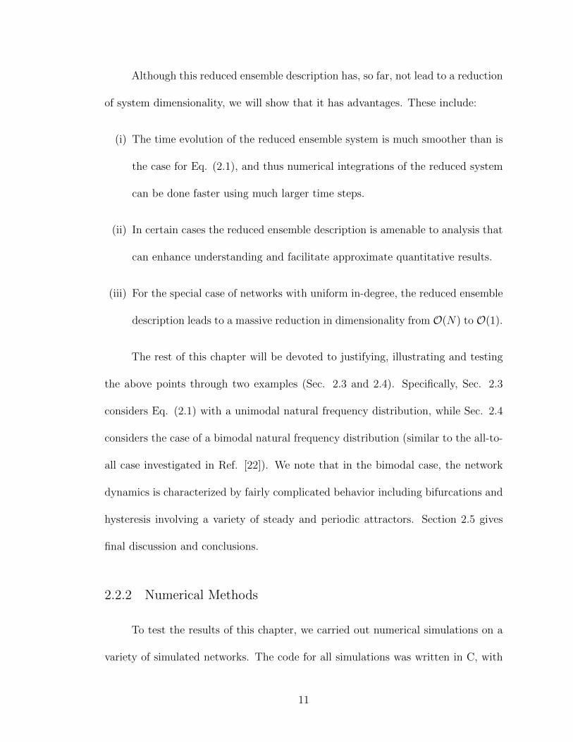
2.2.2 Numerical Methods

To test the results of this chapter, we carried out numerical simulations on a

variety of simulated networks. The code for all simulations was written in C, with

11

parallelization done using either OpenMP to take advantage of multiple CPU cores

(4x 3.2 GHz AMD Phenom II) or CUDA to utilize our Nvidia Tesla C1060 GPGPU

(240x 1.3 GHz stream processors). Any scripts were written in Bash. Eigenspectum

computation was done in Python using the LAPACK package for NumPy.

In performing our numerical simulations, we used three different adjacency

matrices: a directed network of uniform in-degree, an undirected Erdos-Renyi ran-

dom graph and an undirected scale-free network. The same network size, N = 104,

was used throughout.

The uniform in-degree network was generated in such a way as to have an

in-degree din = 100 for all nodes: for each node i, exactly din other discrete nodes

j were randomly selected. For each of those nodes j, Aij was set to 1. The largest

eigenvalue of this matrix is λ1 = din = 100, and each entry of the corresponding

right eigenvector ~u1 is u1i = 1/√N , for the normalization ~uT1 ~u1 = 1.

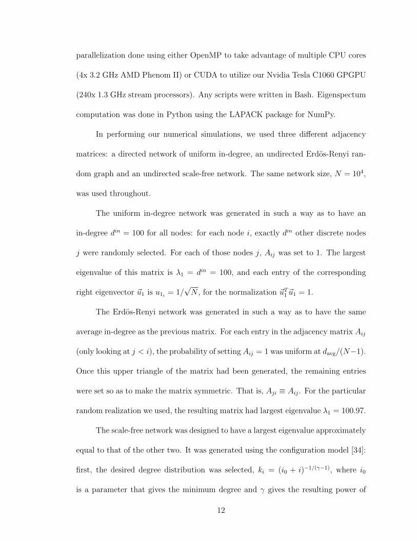
The Erdos-Renyi network was generated in such a way as to have the same

average in-degree as the previous matrix. For each entry in the adjacency matrix Aij

(only looking at j < i), the probability of settingAij = 1 was uniform at davg/(N−1).

Once this upper triangle of the matrix had been generated, the remaining entries

were set so as to make the matrix symmetric. That is, Aji ≡ Aij. For the particular

random realization we used, the resulting matrix had largest eigenvalue λ1 = 100.97.

The scale-free network was designed to have a largest eigenvalue approximately

equal to that of the other two. It was generated using the configuration model [34]:

first, the desired degree distribution was selected, ki = (i0 + i)−1/(γ−1), where i0

is a parameter that gives the minimum degree and γ gives the resulting power of

12

the power-law degree distribution; then, for each entry of the adjacency matrix

Aij, j < i, the probability of setting Aij = 1 was taken to be ckikj where c is a

renormalizing factor that allows us to control the number of edges in the network. As

with the Erdos-Renyi network, once the upper triange of the matrix was generated,

the lower triangle was set so that Aji ≡ Aij. The scale-free matrix we used had

γ = 2.5 and largest eigenvalue λ1 = 100.34.

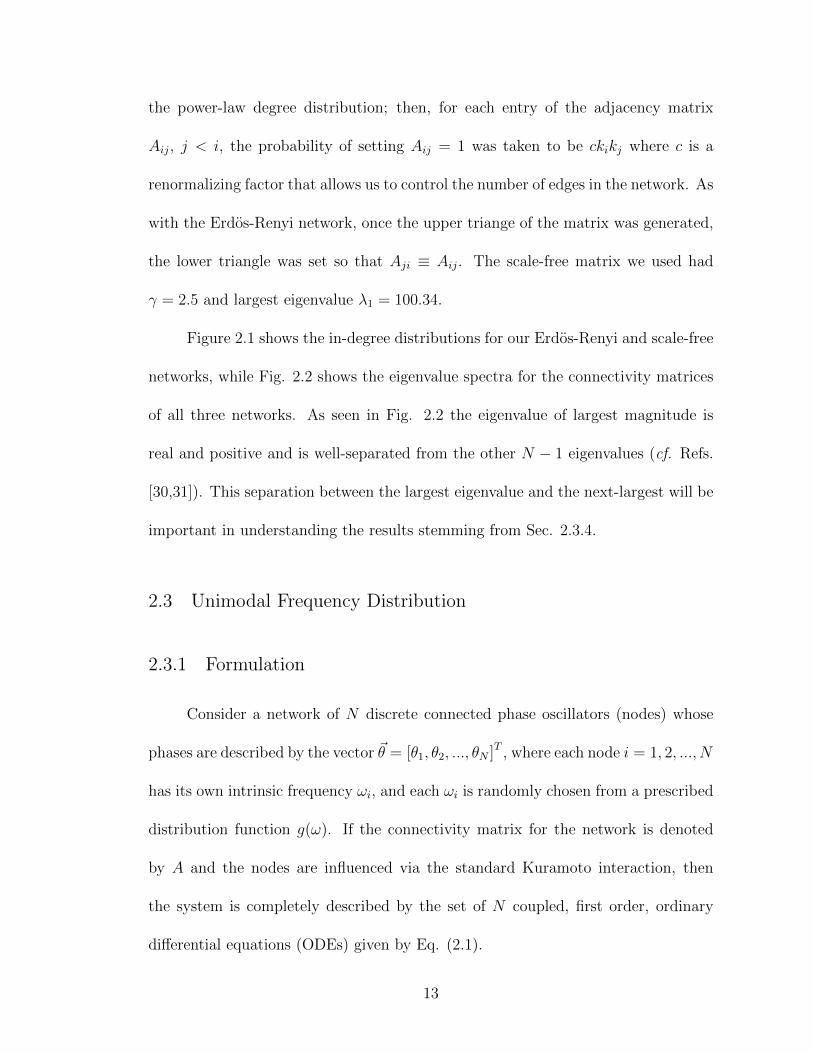
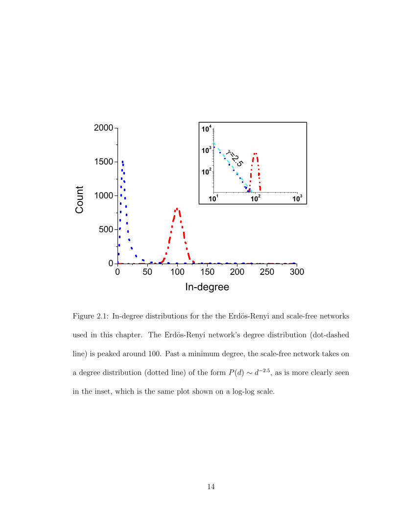
Figure 2.1 shows the in-degree distributions for our Erdos-Renyi and scale-free

networks, while Fig. 2.2 shows the eigenvalue spectra for the connectivity matrices

of all three networks. As seen in Fig. 2.2 the eigenvalue of largest magnitude is

real and positive and is well-separated from the other N − 1 eigenvalues (cf. Refs.

[30,31]). This separation between the largest eigenvalue and the next-largest will be

important in understanding the results stemming from Sec. 2.3.4.

2.3 Unimodal Frequency Distribution

2.3.1 Formulation

Consider a network of N discrete connected phase oscillators (nodes) whose

phases are described by the vector ~θ = [θ1, θ2, ..., θN ]T , where each node i = 1, 2, ..., N

has its own intrinsic frequency ωi, and each ωi is randomly chosen from a prescribed

distribution function g(ω). If the connectivity matrix for the network is denoted

by A and the nodes are influenced via the standard Kuramoto interaction, then

the system is completely described by the set of N coupled, first order, ordinary

differential equations (ODEs) given by Eq. (2.1).

13

0 50 100 150 200 250 3000

500

1000

1500

2000

101 102 103

102

103

104

Cou

nt

In-degree

=2.5

Figure 2.1: In-degree distributions for the the Erdos-Renyi and scale-free networks

used in this chapter. The Erdos-Renyi network’s degree distribution (dot-dashed

line) is peaked around 100. Past a minimum degree, the scale-free network takes on

a degree distribution (dotted line) of the form P (d) ∼ d−2.5, as is more clearly seen

in the inset, which is the same plot shown on a log-log scale.

14

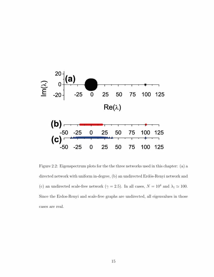
Figure 2.2: Eigenspectrum plots for the the three networks used in this chapter: (a) a

directed network with uniform in-degree, (b) an undirected Erdos-Renyi network and

(c) an undirected scale-free network (γ = 2.5). In all cases, N = 104 and λ1 ' 100.

Since the Erdos-Renyi and scale-free graphs are undirected, all eigenvalues in those

cases are real.

15

Defining the order parameter Ri for each oscillator i,

Ri ≡1

N

N∑j=1

Aijeiθj , (2.2)

we can rewrite Eq. (2.1) as

dθidt

= ωi + kIm[e−iθiRi

]. (2.3)

We now consider an ensemble of systems of the form of Eq. (2.3), where each

member of the ensemble has the same fixed network as specified by its adjacency

matrix A, and each member of the ensemble has a different randomly chosen set of

nodal frequencies ωi. Thus we assume that a randomly chosen system ensemble

member has nodal natural frequencies in the ranges,

ω1 ∈ [ω′1 + dω′1] ,

ω2 ∈ [ω′2 + dω′2] ,

...

ωN ∈ [ω′N + dω′N ] ,

with probability

g(ω′1)g(ω′2)...g(ω′N)dω′1dω′2...dω

′N .

We further envision that at t = 0 the initial angles are given with some probability

distribution,

fN(θ1, θ2, ..., θN ;ω1, ω2, ..., ωN ; 0)

which evolves into the future t ≥ 0 according to the oscillator conservation equation,

∂fN∂t

+N∑i=1

∂

∂θi

[fN θi

]= 0. (2.4)

16

In Eq. (2.4) θi ≡ dθi/dt is given by Eq. (2.3) (note that ωi = 0), and

Ri ≡1

N

N∑j=1

Aij

∫eiθjfNd

NωdNθ,

Ri =1

N

N∑j=1

Aij

∫ ∞−∞

dωj

∫ 2π

0

dθjeiθjfj(θj, ωj, t), (2.5)

where fj is the marginal distribution function

fi(θi, ωi, t) =

∫fN(θj, ωj)

∏j 6=i

dωjdθj. (2.6)

Multiplying Eq. (2.4) by∏

j 6=i dωjdθj and integraing, we find that the marginal

distribution functions satisfy

∂fi∂t

+∂

∂θ(fiθi) =

∂fi∂t

+∂fi∂θ

θi + fi∂θi∂θ

= 0. (2.7)

Note that by use of this formulation we calculate the average behavior of

the oscillator order parameters Ri over the ensemble [Eq. (2.5)] rather than the

oscillator order parameter for a single realization [Eq. (2.2)]. For large systems (in

the limit N → ∞), one expects some degree of self-averaging, so that a suitable

bulk order parameter (such as the one we introduce later in this section) will be the

same, regardless of whether it was calculated from Eqs. (2.2) and (2.3) or from Eqs.

(2.5) and (2.7).

Following Ref. [8], we proceed by seeking a special solution in the particular

assumed form,

fi(θi, ωi, t) =g(ωi)

2π

[1 +

∞∑n=1

(αni (ωi, t)e

inθi + αn∗i (ωi, t)e−inθi

)], (2.8)

where |αi| < 1 is assumed for convergence.

17

Inserting Eq. (2.8) in Eq. (2.7), we find that our special assumed form is a

solution of Eq. (2.7) if

dαidt

+ iαiωi +k

2

[α2iRi −R∗i

]= 0. (2.9)

Furthermore, inserting Eq. (2.8) in Eq. (2.5) yields

Ri =1

N

N∑j=1

Aij

∫ ∞−∞

α∗j (ωj, t)g(ωj)dωj. (2.10)

We now consider the case where g(ω) is Lorentzian,

g(ω) =1

π

∆

(ω − ω0)2 + ∆2=

1

2πi

(1

ω − ω0 + i∆− 1

ω − ω0 − i∆

). (2.11)

It has been shown [8] that, under appropriate restrictions in the initial conditions,

α(ω, t) is bounded and analytic in the lower-half ω-plane. Thus, we can close the

integral in Eq. (2.10) in the lower-half plane to obtain from the pole at ω = ω0− i∆

Ri =1

N

N∑j=1

Aijα∗j (ω0 − i∆, t). (2.12)

We define αi(t) ≡ αi(ω0 − i∆, t) and set ω = ω0 − i∆ in Eq. (2.9) to obtain a

system of N ordinary differential equations, for the quantities αi,

0 =dαi(t)

dt+ i(ω0 − i∆)αi(t) +

k

2

[α2i (t)Ri(t)−R∗i (t)

], (2.13)

Ri =1

N

N∑j=1

Aijα∗j (t). (2.14)

As shown in Ref. [9], the long-time system behavior of Eqs. (2.5) and (2.7) is

attracted to the manifold of solutions of the form of Eq. (2.8), and Eqs. (2.13) and

(2.14) thus describe all possible attractors and bifurcations of the system.

18

By making the transformation αi → αieiω0t, the quantity ω0 is transformed to

zero. With this done, Eqs. (2.13) and (2.14) become consistent with the assumption

that αi and Ri are real, and we obtain

0 =dαi(t)

dt+ ∆αi(t) +

kRi

2

[α2i (t)− 1

], (2.15)

Ri =1

N

N∑j=1

Aijαj(t). (2.16)

While this ensemble formulation of the Kuramoto problem has not resulted in a

decrease in the number of equations compared to the original formulation, Eqs. (2.3)

and (2.2) (which we henceforth refer to as the theta formulation), the set of equations

described in Eqs. (2.15) and (2.16) offer several advantages. One advantage is

that the system described by our ensemble formulation equations is more “robust,”

owing to the fact that the ensemble formulation equations, by their nature, average

over a range of initial conditions. Computationally, as shown in Figs. 2.3-2.5,

whereas the theta formulation equations require many trials to produce smooth

data, the ensemble formulation equations require only one, and may be run using

larger timesteps: generally, we found that for ensemble formulation simulations, we

could use a time step size ten times larger than the one required for theta formulation

simulations.

Another advantage of our ensemble formulation equations is that they fa-

cilitate analysis of the system. In particular, in Secs. 2.3.3 and 2.3.4 we will use

these equations to obtain information about the fixed-point attractors of the system.

Furthermore, in Sec. 2.3.5 we will demonstrate, for the case of uniform in-degree, a

reduction of the full system [Eq. (2.15)] of N ODEs to a single ODE.

19

2.3.2 Bulk Order Parameter

In describing the behavior of the system, we are more concerned with the

aggregate behavior, rather than, say, the individual order parameters Ri (as given

by Eq. (2.2) and equivalently by Eq. (2.5)). Thus, we define an average order

parameter for the entire network,

r ≡ |~vT1 ~R|, (2.17)

where ~v1 is the left eigenvector of the adjacency matrix A corresponding to its

eigenvalue of largest magnitude, and is normalized so that ~vT1 ~u1 = ~uT1 ~u1 = 1, where

~u1 is the associated right eigenvector. The reason for this choice of order parameter

will be made more clear in Sec. 2.3.4.

Figures 2.3-2.5 shows the time-evolution of r for simulations carried out on

the three networks introduced in Sec. 2.2.2, for a selection of coupling strengths

k. For the theta formualtion simulations the initial values of θi were random in

[0, 2π); for the ensemble formulation the αi(0) were set to zero, save α1, which was

initialized small compared to one; to compare the time evolutions, the ensemble

formulation curves in Figs. 2.3-2.5 were horizontally shifted to most closely match

those of the theta formulation. For all three networks, the ensemble formulation

simulations reproduces the results for the theta formulation simulations: not only

does r asymptote to the same values, but the evolution takes the same shape, ac-

curately reproducing the transient rise to synchrony. The agreement between the

theta and ensemble formulation results is best when r is large, as there is noise

20

inherent to the theta formulation results. Note that, as previously claimed, these

ensemble formulation computations can be carried out at larger time step than the

theta formulation computations, and thus are much faster.

2.3.3 Steady State

Setting dαi/dt = 0, Eq. (2.15) gives the quadratic equation,

0 = α2i − 1 +

2∆

kRi

αi. (2.18)

With the requirement that |αi| ≤ 1, we have the solution,

αi =

√∆2

k2R2i

+ 1− ∆

kRi

. (2.19)

Inserting this into Eq. (2.16), we obtain a system of N transcendental equations for

the oscillator order parameters,

Ri =1

N

N∑j=1

Aij

(√∆2

k2R2j

+ 1− ∆

kRj

). (2.20)

Equations (2.20) can be solved numerically by inserting an initial guess for

Rj on the right side, calculating the new Ri and iterating this process. This

results in steady state values of Ri with much less computation than would be

necessary if the same information were obtained using either our theta formulation

or ensemble formulation equations.

Our Eq. (2.20) agrees with Eq. (14) of Ref. [13] for g(ω) Lorentzian. How-

ever, our derivation followed without approximation once the ensemble viewpoint

is adopted, while Eq. (14) of Ref. [13] was derived using approximations that, al-

though reasonable, are not easy to justify in a rigorous way. On the other hand,

21

0 10 20 30 40 500.0

0.5

1.0

0 10 20 30 40 500.0

0.5

1.0

0 25 50 75 1000.0

0.1

0.2

(a)

(b)

r(t)

t

(c)

Figure 2.3: Bulk order parameter r vs. time for systems simulated using the theta

formulation (Eqs. (2.1) and (2.2)) as well as our ensemble formulation (Eqs. (2.15)

and (2.16)), performed on the networks introduced in Sec. 2.2.2: (a) uniform in-

degree, (b) Erdos-Renyi and (c) scale-free. Results were generated numerically using

a fourth-order Runge-Kutta integration scheme with fixed time step. Each curve

represents a single simulation–no curves are averaged. A time step ∆t = 0.1 was used

for all theta formulation simulations, save for the scale-free, for which ∆t = 0.05

was used, while all ensemble formulation simulations used a time step ten times

larger than was used for the corresponding theta formulation simulations. The

width of the frequency distribution was set to ∆ = 0.1 and the coupling strength to

k = 50 ' 2.5kc.

22

0 50 100 1500.0

0.2

0.4

0.6

0 50 100 1500.0

0.2

0.4

0.6

0 50 100 1500.00

0.05

0.10

(a)

(b)

r(t)

t

(c)

Figure 2.4: Same as Fig. 2.3 but with k = 30 ' 1.5kc

the result of (14) of Ref. [13] is for a general distribution of g(ω) and is not limited

to the Lorentzian. Thus we regard our result [Eq. (2.20)] and that of Ref. [13] as

being complementary and reinforcing of each other.

In addition to direct numerical solution of Eq. (2.20), Eq. (2.20) can also be

used as a basis for further analysis. In this latter regard we now use Eq. (2.20) to

obtain the critical coupling strength k = kc, such that, for k < kc, Ri → 0 (i.e.,

the network oscillator phases are incoherent) while for k > kc, coherence emerges.

Expanding Eq. (2.20) to first order in kRj/∆ << 1, we obtain

~R ' k

2N∆A~R, (2.21)

where ~R = [R1, R2, ..., RN ]T . This is an eigenvalue problem, and so the smallest

23

0 50 100 150 2000.00

0.25

0.50

0 50 100 150 2000.00

0.25

0.50

0 50 100 150 200 250 3000.00

0.05

0.10

(a)

(b)

r(t)

t

(c)

Figure 2.5: Same as Figs. 2.3 and 2.4 but with k = 25 ' 1.25kc

coupling strength to have a nonzero solution to this equation will occur for the

largest eigenvalue of A, which we will denote λ1. Thus, as previously found in Ref.

[13], the critical coupling strength is

kc =2N∆

λ1

. (2.22)

2.3.4 Maximum Eigenvalue Approximation

In order to investigate steady state behavior for k > kc, we assume that the

eigenvalues of A are distinct and decompose A into the sum,

A =N∑k=1

λk~uk~vTk , (2.23)

24

where ~uk and ~vk are, respectively, the sets of right and left eigenvectors of A and

λk is the set of corresponding eigenvalues (the eigenvectors are normalized such

that ~vTl ~uk = δkl and |~uk| = 1). Since all entries of the adjacency matrix are non-

negative, the Perron-Frobenius theorem suggests that there is a unique eigenvalue of

largest magnitude, which is real and positive. Assuming that this largest eigenvalue

is much larger than all the others, we consider only the first term in Eq. (2.23),

A ' λ1~u1~vT1 . (2.24)

As shown in Fig. 2.2, we expect this approximation to be more appropriate for

our uniform in-degree network and our Erdos-Renyi graphs, where λ1 is larger than

the magnitude of the second largest eigenvalue λ2 by a factor of 9.93 and 5.05,

respectively, and less so for the scale-free network, where the ratio is only 1.89.

Using Eq. (2.24) in Eq. (2.16) implies that ~R is approximately parallel to ~u1,

and thus we define a scalar ρ by

~R = ρ~u1, (2.25)

where, again using Eq. (2.16), ρ is

ρ ≡ λ1

N

N∑i=1

v1iαi(t) (2.26)

Note that ~vT1 ~R = ρ~vT1 ~u1 = ρ. Thus, as long as the maximum eigenvalue approxima-

tion [Eq. 2.24)] holds, our bulk order parameter [Eq. (2.17)] is given by r = ρ.

Using Eq. (2.25) in Eq. (2.20), we obtain to a single transcendental equation

for ρ,

ρ2 =λ1

N

N∑j=1

v1j

u1j

(√∆2

k2+ ρ2u2

1j− ∆

k

)(2.27)

25

As shown in Fig. 2.6, this solution matches the steady-state results of running

lengthy theta formulation or ensemble formulation simulations only to the extent

that the maximum eigenvalue approximation holds. Specifically, we see excellent

agreement for our uniform in-degree and Erdos-Renyi networks, while, for scale-free

networks, for which the maximum eigenvalue approximation does not hold well, we

see discrepancies.

From Eq. (2.27), we can obtain an upper bound to our bulk order parameter

by considering the limit where ∆/k → 0,

ρmax =λ1

N

N∑j=1

v1j . (2.28)

We note that for the uniform in-degree and Erdos-Renyi networks, each entry of

the right eigenvalue u1i is approximately equal, and thus, due to normalization,

approximately equal to 1/√N . Since ~vT1 u1 = 1, this implies that the sum in Eq.

(2.28) is approximately equal to√N and thus, ρmax ' λ1/

√N . We further note

that this does not hold for the scale-free case.

Equation (2.27) may be further simplified if we define ξ ≡ ρ2k2/∆2. In terms

of this new quantity,

ξ =2k

kc

N∑j=1

v1j

u1j

(√1 + ξu2

1j− 1)≡ k

kcF (ξ). (2.29)

We remark that one can show that the function F (ξ) in Eq. (2.29) has F (0) = 0,

F ′(0) = 1, F ′′(ξ) < 0 and increases as√ξ for large positive ξ. As illustrated in Fig.

2.7, these properties imply that Eq. (2.29) has no positive solutions if k < kc and

exactly one positive solution if k > kc.

26

50 100 150 2000.0

0.2

0.4

0.6

0.8

1.0max=1.000

max=1.005

r(k)

k

max=0.5082

k c=20

Figure 2.6: Long-time-averaged values of r vs. k for systems simulated using the

theta formulation [Eqs. (2.1) and (2.2)] and for identical systems simulated us-

ing our ensemble formulation [Eqs. (2.15) and (2.16)] and ρ calculated from the

transcendental equation (Eq. (2.27)). Also shown as dashed lines are the critical

coupling value kc, which is approximately the same for all three networks, and the

values of ρmax [Eq. (2.28)] for the three networks. The same integration scheme

was used as for Figs. 2.3-2.5. Simulations were generally run for 300 time units for

the theta formulation simulations, with averaging done over the last 50 time units,

while the ensemble formulation simulations were run until they converged (generally

between 200 and 500 time units). Selected points were rerun at smaller time step

size and longer simulation runtime to ensure validity.

27

2 4 6 8 100

2

4

6

8

10k c/k>1

F()/N

/N

k c/k<1

F(

Figure 2.7: F (ξ)/N and (kc/k)ξ vs. ξ/N for two different values of kc/k. When

kc/k > 1, there is no nonzero intersection of the two curves (thus, no nonzero

solution to Eq. (2.29)).

28

2.3.5 Special case: Uniform in-degree

In the case of networks with uniform in-degree, din =∑

j Aij independent of

i, Eqs. (2.15) and (2.16) admit a special solution,

α1(t) = α2(t) = ... = αN(t) ≡ α(t). (2.30)

Restricting Eqs. (2.15) and (2.16) to this manifold yields

1

∆

dα

dt+ α +

kdin

2N∆

(α2 − 1

)α = 0. (2.31)

If we define K ≡ (kdin)/(N∆), Eq. (2.31) becomes identical to Eq. (10) of Ref. [8]

which was derived for the all-to-all coupled case. As noted in Ref. [8], the solution

to Eq. (2.31) is

α(t)

α∞=

1 +

[(α∞α0

)2

− 1

]exp

[1− K

2∆t

]−1/2

, (2.32)

where

α∞ =

√1−

(2

K

)(2.33)

is the value that α(t) approaches as t → ∞ when k > kc (that is, K > 2). Note

that this same value of α∞ follows from the solution of Eq. (2.20) in the uniform

in-degree case with all the Ri set equal. To test the relevance of Eq. (2.32), we

compare its prediction for r(t) with that from solution of Eq. (2.15) for k > kc,

where we initialize Eq. (2.15) with~α(0) far from the manifold given by Eq. (2.30) by

setting α1(0) to some nonzero value (α1(0) = 1) and α2(0) = α3(0) = ...αN(0) = 0.

Adjusting α(0) in Eq. (2.32) to provide the best apparent fit, we obtain the results

for r(t) plotted in Fig. 2.8. The good agreement between Eq. (2.32) (solid line in

29

0 50 100 150 200 250 3001E-8

1E-7

1E-6

1E-5

1E-4

1E-3

0.01

0.1

1

D(t)

t0.0

0.1

0.2

0.3

0.4

0.5

0.6

r(t)

Figure 2.8: Bulk order parameter r vs. t for our uniform in-degree network simulated

using our ensemble formulation [Eqs. (2.15) and (2.16)] (dashed line) plotted with

ρ calculated from Eq. (2.32) (solid line). The normalized L2 deviation, D, from the

manifold given by Eq. (2.30) is also plotted (dotted line) along with the slope given

by Eq. (2.41) (dash-dotted line).

Fig. 2.8) and Eq. (2.15) (dashed line) indicate that the solutions to Eq. (2.15) are

rapidly attracted to the solution manifold [Eq. 2.30]. This is further confirmed by

computation of the normalized L2 deviation of ~α from the equal-α manifold, which

we define by

D ≡

√∑i (αi − α)2∑

i α2i

, (2.34)

where α =∑

i αi/N . The evolution of D is plotted as a dotted line in Fig.

2.8. It is seen that, after about t = 60, D(t) decreases exponentially with time

30

(as indicated by the linear dependence on the semi-log plot of Fig. 2.8), reaching

the level of numerical roundoff by t ' 150. Although the curves in Fig. 2.8 are

for a difected network, to explain this exponential decrease, it is somewhat simpler

to consider an undirected network, in which case AT = A, λk is real, ~vk = ~uk,

~uTk ~ul = δkl, and we use the convention, λk ≥ λk+1. We note that for uniform in-

degree, λ1 = din and the elements of ~u1 are all equal. Thus, ~u1 corresponds to the

manifold given by Eq. (2.30), and, by the orthogonality condition (~uTk ~u1 = 0 for

k ≥ 2), all other eigen-directions are perpendicular to the manifold. Writing ~α in

the eigenvalue basis, we have

~α(t) =N∑k=1

ak(t)~uk, (2.35)

with ak(0) = ~uTk ~α(0). Thus we obtain

D =

√∑Nk=2 a

2k∑N

k=1 a2k

(2.36)

Initially the components of ~α are small and we may linearize Eq. (2.15) to obtain

d~α

dt+ ∆~α− k

2NA~α = 0. (2.37)

Inserting Eq. (2.35) into Eq. (2.37) we have

ak(t) = ak(0)eγkt (2.38)

and

γk(t) =kλk2N−∆. (2.39)

Since γk ≥ γk+1, after an inital phase, the sums in Eq. (2.36) are dominated by

their first terms,

D(t) ' |a1(t)||a2(t)|

= c exp [− (γ1 − γ2) t], (2.40)

31

where c is a constant. Thus we see that D(t) should decrease exponentially at the

rate

(γ1 − γ2) = k(din − λ2)/(2N). (2.41)

For the case in Fig. 2.8 (din = 100, λ2 = 9.94) this predicted slope is plotted as the

dash-dotted line segment and is seen to yield excellent agreement with the slope of

the dotted curve.

2.4 Bimodal Frequency Distribution

2.4.1 Formulation

We now turn our attention to the case where, instead of a single-peaked

Lorentzian for our frequency distribution g(ω), we choose a bimodal distribution,

g(ω) =∆

2π

(1

(ω − ω0)2 + ∆2+

1

(ω + ω0)2 + ∆2

). (2.42)

In this case, when we close the integral∫∞−∞ α

∗gdωj, in the lower-half plane, we

encircle two poles, one at ω = +ω0− i∆ and one at ω = −ω0− i∆. Thus we obtain

two residue contributions,

Ri =1

2N

N∑j=1

Aij[α∗j (ω0 − i∆, t) + α∗j (−ω0 − i∆, t)

]. (2.43)

Evaluating Eq. (2.9) at our two poles, we obtain a set of 2N ODEs,

α±i ≡dα±idt

= −(∆± iω0)α±i +k

2

[R∗i −Ri(α

±i )2], (2.44)

where we have defined

α±i (t) ≡ αi(±ω0 − i∆, t). (2.45)

32

2.4.2 Uniform In-degree

Similar to the analysis in Sec. 2.3.5, by assuming that the network has uniform

in-degree din =∑

j Aij where din is independent of i, one finds that one can obtain

an exact special solution of Eq. (2.44) by setting

α±i = α±j ≡ α±, (2.46)

in which case the system of 2N ODEs given by Eq. (2.44) reduces to a system of

only two ODEs:

ρ± = −(∆∓ iω0)ρ± +kdin

4N

[(ρ+ + ρ−

)− 4N

(din)2

(ρ±)2 (

ρ+ + ρ−)∗]

, (2.47)

where

ρ± ≡ din

2√N

(α±)∗. (2.48)

Introducing polar coordinates, ρ± = a± exp (iφ±), we obtain three real ODEs,

a± = −∆a± +kdin

4N

(1− 4N

(din)2

(a±)2)(

a± + a∓ cosψ), (2.49)

where ψ ≡ φ+ − φ−, and

ψ = 2ω0 −kdin

4N

[a+

a−+a−

a++

8N

(din)2a+a−

]sinψ. (2.50)

Thus the set of 2N complex first order ODEs [Eq. (2.44)] reduces to a set of just

three real ODEs [Eqs. (2.49) and (2.50)].

If we further assume that the solutions of interest obey the symmetry a+ =

a− ≡ a, then the equations simplify further, from 3 ODEs to 2 ODEs,

a = akdin

4N

[1− 4N∆

kdin− 4N

(din)2a2 + (1− 4N

(din)2a2) cosψ

](2.51)

33

and

ψ = 2ω0 −kdin

2N

[1 +

4N

(din)2a2

]sinψ. (2.52)

These equations are equivalent to Eqs. (22) and (23) of Ref. [22], in the case where

din = N (representing global all-to-all coupling).

To relate a and ψ to the bulk order parameter used in previous sections, we

note that, from Eqs. 2.26 and 2.48,

ρ = ρ+ + ρ−

(with r ' ρ as long as the Maximum Eigenvalue approximation holds). From our

definitions of a and ψ, then, we find that

ρ = 2a cosψ/2 (2.53)

if we assume that ρ is real.

We stress that, while this is a solution to the reduced system, the ansatz

expressed in Eq. (2.46) (as well as the symmetry a+ = a−) has yet to be justified. In

particular, assuming that, by solving Eqs. (2.51) and (2.52), we have found solutions

α±i = α± of the system of Eq. (2.44), one can ask what happens if we add in small

perturbations δα±i to this solution; that is, we set α±i = α±+δα±i . Substituting these

perturbed states into Eq. (2.44), we can linearize to obtain evolution equations for

the perturbations. If these perturbations grow exponentially with time, then our

solutions are unstable and are not expected to exist in typical situations. This

problem is analogous to that of the stability of the synchronization manifold of

coupled chaotic systems, often studied by the master stability function technique

34

[37, 38]. Here we leave the study of the linearized equations for the quantitites δα±i

as a problem for further study. However, Fig. 2.9 supports the idea that this ansatz

is stable. Figure 2.9 plots r(t) for a simulation using the theta formulation for a

network with uniform in-degree and for a simulation using Eqs. (2.51) and (2.52).

Values for the various parameters were chosen such that the system converged to

a limit cycle attractor. The excellent agreement between the two curves at large

times, both in magnitude and period of oscillation, indicates that, even if the system

did not start on the manifold of Eq. (2.46), then it converged onto it.

In Sec. 2.4.3 we further address the question of the stability of the ansatz

(2.46) by comparing long-time solutions of Eqs. (2.51) and (2.52) with full theta

formulation simulations [Eq. (2.1)]. As shown in Sec. 2.4.3, these simulations

confirm that the manifold (2.46) in the full state space of Eq. (2.44) is stable, and

moreover, globally attracting.

2.4.3 Dynamics

We may rescale the parameters of Eqs. (2.51) and (2.52) to make the equations

independent of K, N and din by defining

∆ ≡ 4N∆/(kdin), (2.54)

ω0 ≡ 4Nω0/(kdin), (2.55)

t ≡ kdint/(4N) (2.56)

and

a ≡ 2√Na/din, (2.57)

35

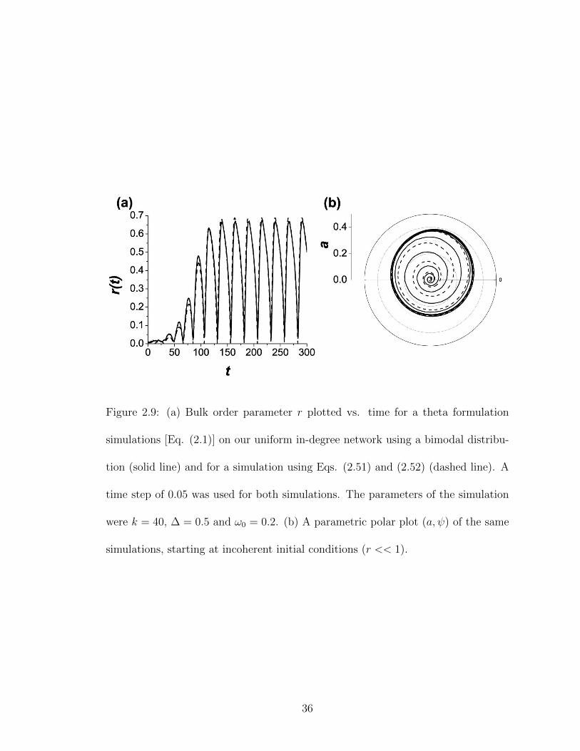
Figure 2.9: (a) Bulk order parameter r plotted vs. time for a theta formulation

simulations [Eq. (2.1)] on our uniform in-degree network using a bimodal distribu-

tion (solid line) and for a simulation using Eqs. (2.51) and (2.52) (dashed line). A

time step of 0.05 was used for both simulations. The parameters of the simulation

were k = 40, ∆ = 0.5 and ω0 = 0.2. (b) A parametric polar plot (a, ψ) of the same

simulations, starting at incoherent initial conditions (r << 1).

36

in which case Eqs. (2.51) and (2.52) become:

da

dt= a

[1− ∆− a2 +

(1− a2

)cosψ

](2.58)

and

dψ

dt= 2

[ω0 −

(1 + a2

)sinψ

](2.59)

The dynamics of Eqs. (2.58) and (2.59) have been thoroughly documented in Ref.

[22]. Whereas the unimodal problem only exhibited fixed point solutions, the bi-

modal case allows for such phenomena as hysteresis and limit cycle attractors. These

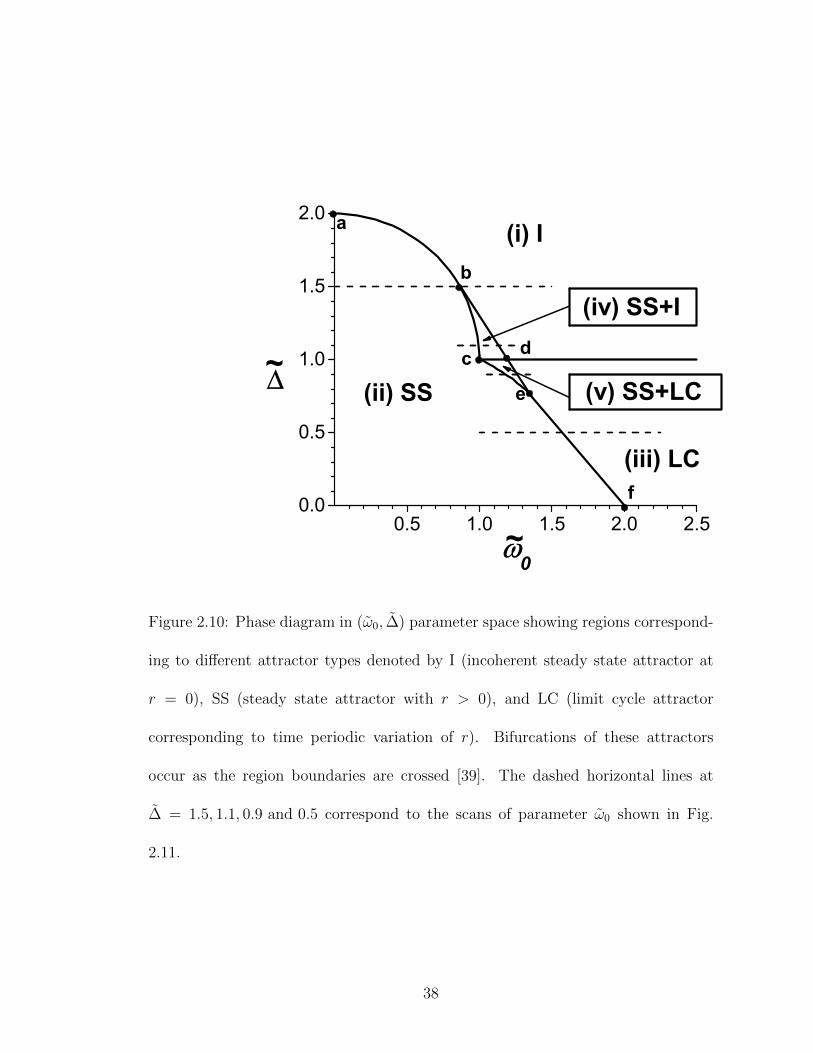
dynamics are summarized in our Fig. 2.10, which is similar to Fig. 2. of Ref. [22].

In Fig. 2.10 we show five distinct regions [labeled (i)-(v)]. For each of the five regions

in Fig. 2.10, we have indicated the type of attractor (or types of attractors) that

exist in that region using the following notations: I for incoherent, corresponding to

a steady state at r = 0; SS for coherent steady state, corresponding to a constant

nonzero attracting value of r; and LC for a limit cycle attractor for which r varies

periodically in time. Note that regions (i)-(iii) are characterized by the presence

of a single unique attractor, while regions (iv) and (v) each have two coexisting

attractors (SS and I for (iv); LC and SS for (v)). Thus we expect hysteresis to be

associated with parameter scans passing through regions (iv) and (v).

Figure 2.11 shows the results of a series of numerical simulations, scanning

across a range of values for ω0, while limiting ∆ to one of four values and keeping

the coupling constant fixed at k = 40 (the four dashed lines in Fig. 2.10). These

plots show the long time system behavior of the bulk order parameter r defined in

Eq. (2.17). Vertical dashed lines indicate the values of ω0 where a scan crosses one of

37

0.5 1.0 1.5 2.0 2.50.0

0.5

1.0

1.5

2.0

c

f

d

b

e (v) SS+LC

(iv) SS+I

(iii) LC

(ii) SS~

0~

(i) Ia

Figure 2.10: Phase diagram in (ω0, ∆) parameter space showing regions correspond-

ing to different attractor types denoted by I (incoherent steady state attractor at

r = 0), SS (steady state attractor with r > 0), and LC (limit cycle attractor

corresponding to time periodic variation of r). Bifurcations of these attractors

occur as the region boundaries are crossed [39]. The dashed horizontal lines at

∆ = 1.5, 1.1, 0.9 and 0.5 correspond to the scans of parameter ω0 shown in Fig.

2.11.

38

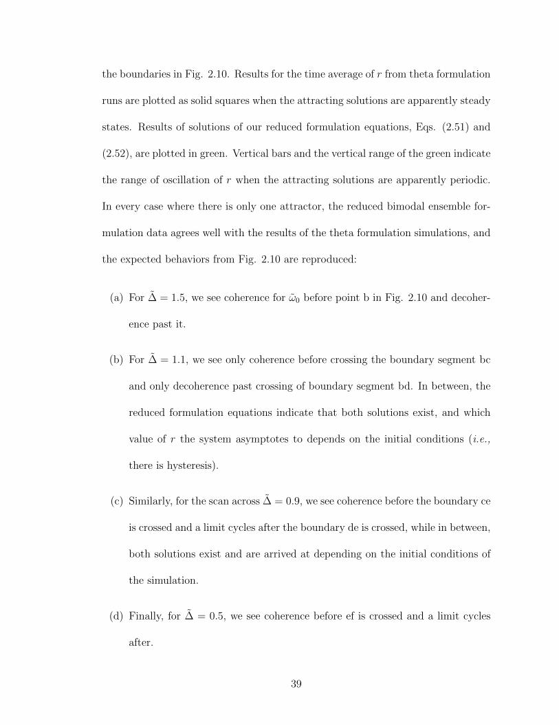
the boundaries in Fig. 2.10. Results for the time average of r from theta formulation

runs are plotted as solid squares when the attracting solutions are apparently steady

states. Results of solutions of our reduced formulation equations, Eqs. (2.51) and

(2.52), are plotted in green. Vertical bars and the vertical range of the green indicate

the range of oscillation of r when the attracting solutions are apparently periodic.

In every case where there is only one attractor, the reduced bimodal ensemble for-

mulation data agrees well with the results of the theta formulation simulations, and

the expected behaviors from Fig. 2.10 are reproduced:

(a) For ∆ = 1.5, we see coherence for ω0 before point b in Fig. 2.10 and decoher-

ence past it.

(b) For ∆ = 1.1, we see only coherence before crossing the boundary segment bc

and only decoherence past crossing of boundary segment bd. In between, the

reduced formulation equations indicate that both solutions exist, and which

value of r the system asymptotes to depends on the initial conditions (i.e.,

there is hysteresis).

(c) Similarly, for the scan across ∆ = 0.9, we see coherence before the boundary ce

is crossed and a limit cycles after the boundary de is crossed, while in between,

both solutions exist and are arrived at depending on the initial conditions of

the simulation.

(d) Finally, for ∆ = 0.5, we see coherence before ef is crossed and a limit cycles

after.

39

0.0 0.5 1.0 1.50.0

0.5

1.0

0.8 1.0 1.20.0

0.5

1.0

1.0 1.1 1.2 1.30.0

0.5

1.0

1.0 1.5 2.00.0

0.5

1.0 (d) =0.5(c) =0.9

(b) =1.1

r

~~

~

~

r

0~

(a) =1.5~

0

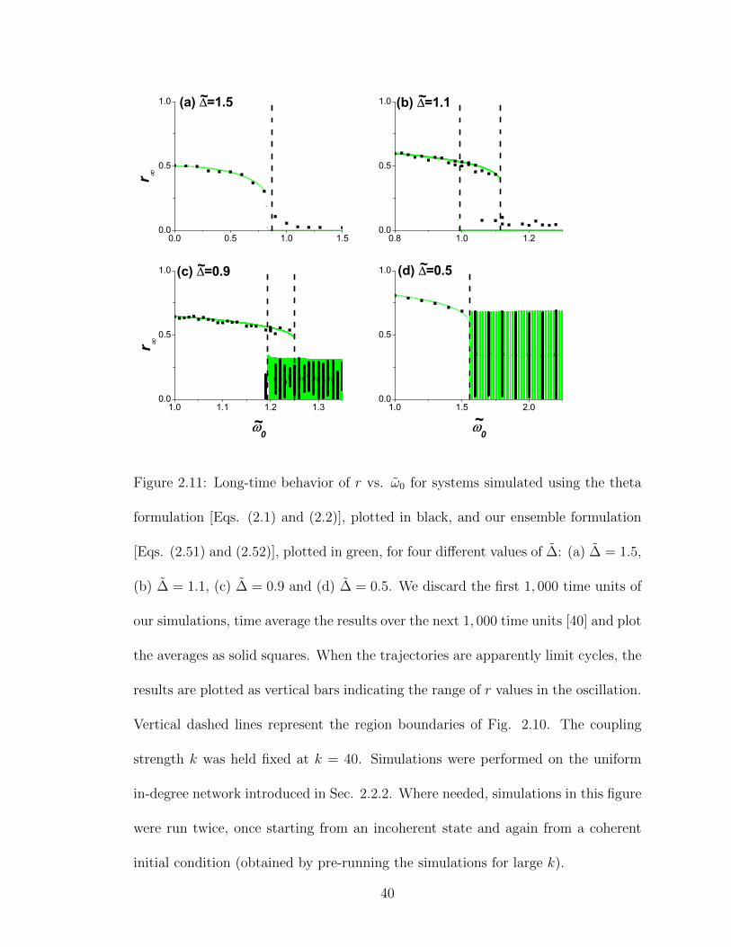
Figure 2.11: Long-time behavior of r vs. ω0 for systems simulated using the theta

formulation [Eqs. (2.1) and (2.2)], plotted in black, and our ensemble formulation

[Eqs. (2.51) and (2.52)], plotted in green, for four different values of ∆: (a) ∆ = 1.5,

(b) ∆ = 1.1, (c) ∆ = 0.9 and (d) ∆ = 0.5. We discard the first 1, 000 time units of

our simulations, time average the results over the next 1, 000 time units [40] and plot

the averages as solid squares. When the trajectories are apparently limit cycles, the

results are plotted as vertical bars indicating the range of r values in the oscillation.

Vertical dashed lines represent the region boundaries of Fig. 2.10. The coupling

strength k was held fixed at k = 40. Simulations were performed on the uniform

in-degree network introduced in Sec. 2.2.2. Where needed, simulations in this figure

were run twice, once starting from an incoherent state and again from a coherent

initial condition (obtained by pre-running the simulations for large k).

40

We note that our numerical theta formulation data in Fig. 2.11(b) does not

show all the attractors across the entire hysteretic range of region (iv). In Fig.

2.11(b), both solutions are observed for the theta formulation simulations only to-

wards the right edge of region (iv). Since the ensemble formulation equations capture

both attractors, we postulate that the incoherent attractor can be close enough to

its basin boundary that the noise inherent in the theta formulation simulations is

enough to knock the system into the coherent attractor for most values of ω0 in the

left part of region (iv).

Support for this view is provided in Figs. 2.12 and 2.13. Figures 2.12(a)

and 2.13(a) show polar polots in (a, ψ) of orbits of our reduced formulation with

the inital value of a set to a = 0.5 for different initial values of ψ in the case

where ∆ = 1.1, corresponding to Fig. 2.11(b). Figure 2.12 is for ω0 = 1.10 and

Fig. 2.13 is for ω0 = 1.05. Orbits tending to the I attractor are plotted (cf. Fig.

2.11b) as red curves, while orbits lending to the SS attractor are plotted as blue

curves. Grey dots mark the attractors and a saddle point. Note that the basin

of the I attractor is substantially smaller at ω0 = 1.05 (Fig. 2.13(a)) as compared

to ω0 = 1.10 (Fig. 2.12(a)). Also, note that the boundary separating these two

attractors is apparently the stable manifold of a saddle steady state and that the

left and right arms of the saddle’s unstable manifold go directly to the I and SS

attractors, respectively. Figures 2.12(b) and (c) show blown up regions centered

around the SS attractor (Fig. 2.12(b)) and around the I attractor (Fig. 2.12(c)),

where the regions are indicated by the rectangles in Fig. 2.12(a). The black curves

plotted in Figs. 2.12(b and c) correspond to the theta formulation orbits initialized

41

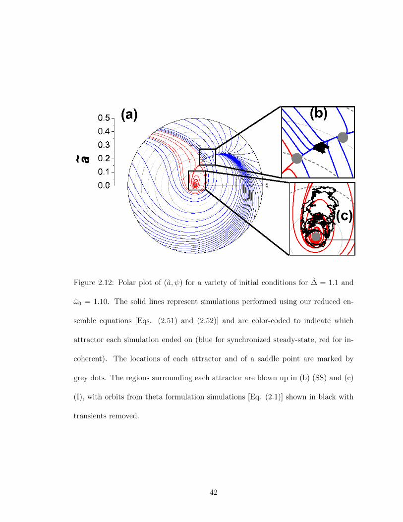
Figure 2.12: Polar plot of (a, ψ) for a variety of initial conditions for ∆ = 1.1 and

ω0 = 1.10. The solid lines represent simulations performed using our reduced en-

semble equations [Eqs. (2.51) and (2.52)] and are color-coded to indicate which

attractor each simulation ended on (blue for synchronized steady-state, red for in-

coherent). The locations of each attractor and of a saddle point are marked by

grey dots. The regions surrounding each attractor are blown up in (b) (SS) and (c)

(I), with orbits from theta formulation simulations [Eq. (2.1)] shown in black with

transients removed.

42

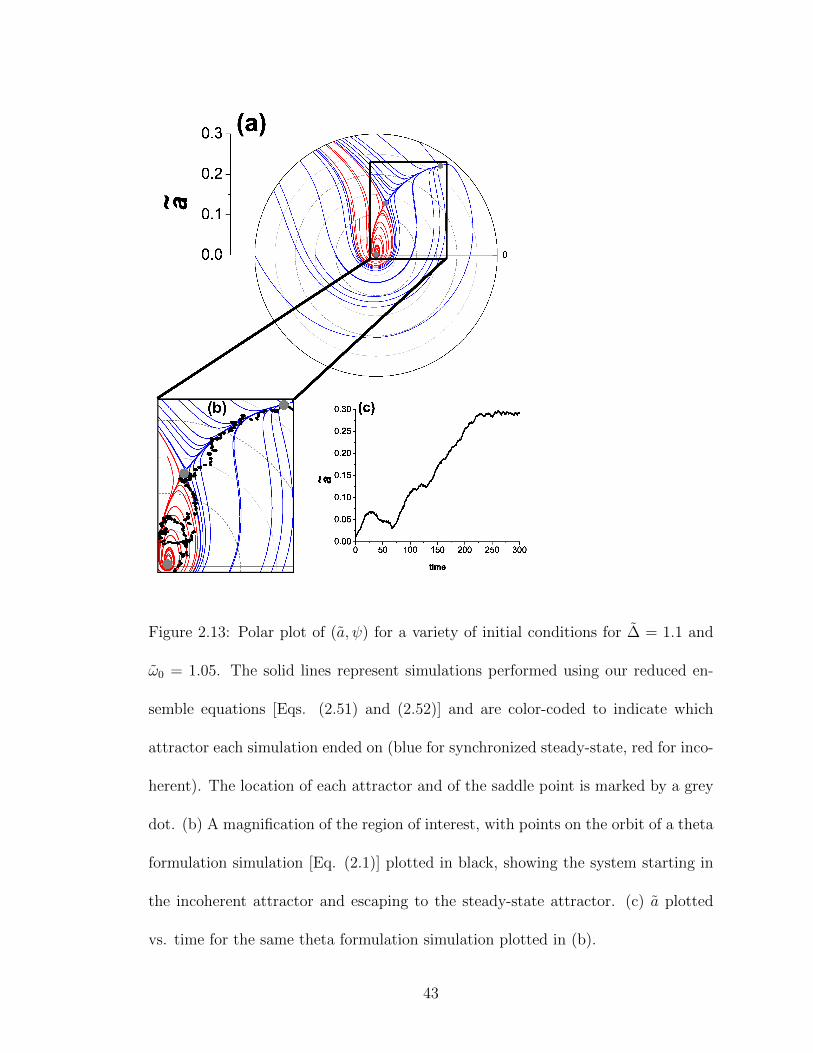
Figure 2.13: Polar plot of (a, ψ) for a variety of initial conditions for ∆ = 1.1 and

ω0 = 1.05. The solid lines represent simulations performed using our reduced en-

semble equations [Eqs. (2.51) and (2.52)] and are color-coded to indicate which

attractor each simulation ended on (blue for synchronized steady-state, red for inco-

herent). The location of each attractor and of the saddle point is marked by a grey

dot. (b) A magnification of the region of interest, with points on the orbit of a theta

formulation simulation [Eq. (2.1)] plotted in black, showing the system starting in

the incoherent attractor and escaping to the steady-state attractor. (c) a plotted

vs. time for the same theta formulation simulation plotted in (b).

43

near the I attractor and near the SS attractor. We see that, although the points stay

near their attractors, there is noticeable scatter reflecting the existence of noise.

In Figs. 2.13(b) and (c), we plot points on a theta formulation simulation orbit

that was initialized incoherently. As shown, although this orbit initially stays close

to the I attractor, it is eventually kicked by noise fluctuations into the SS basin

in the vicinity of the boundary saddle and then goes to the SS attractor closely

following the right arm of the saddle’s unstable manifold. Furthermore, we note

that this mode of escape from the I attractor to the SS attractor is characteristic of

what is to be expected in a noisy environment [41].

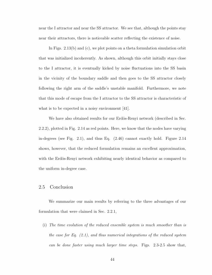
We have also obtained results for our Erdos-Renyi network (described in Sec.

2.2.2), plotted in Fig. 2.14 as red points. Here, we know that the nodes have varying

in-degrees (see Fig. 2.1), and thus Eq. (2.46) cannot exactly hold. Figure 2.14

shows, however, that the reduced formulation remains an excellent approximation,

with the Erdos-Renyi network exhibiting nearly identical behavior as compared to

the uniform in-degree case.

2.5 Conclusion

We summarize our main results by referring to the three advantages of our

formulation that were claimed in Sec. 2.2.1,

(i) The time evolution of the reduced ensemble system is much smoother than is

the case for Eq. (2.1), and thus numerical integrations of the reduced system

can be done faster using much larger time steps. Figs. 2.3-2.5 show that,

44

0.8 1.0 1.20.0

0.5

1.0

1.0 1.1 1.2 1.30.0

0.5

1.0

~

(b) =0.9

r

~

(a) =1.1

~

r

0

Figure 2.14: Two of the graphs from Fig. 2.11 re-plotted to include simulations

done on the Erdos-Renyi network (red) introduced in Sec. 2.2.2.

45

especially at larger values of r, our ensemble formulation reproduces the dy-

namics of the theta formulation. This result was obtained using a time step

ten times larger than that used for each theta formulation simulation, thus

drastically reducing runtime. At small values of r, our results suggest that

the noise inherent to the theta formulation simulations is dominant over the

dynamics. Thus, to obtain usable data in this regime with the theta formula-

tion simulations would require averaging multiple runs. In contrast, ensemble

formulation simulations are effectively noiseless, requiring no averaging.

(ii) In certain cases the reduced ensemble description is amenable to analysis that

can enhance understanding and facilitate approximate quantitative results. In

Sec. 2.3.3, we solve our ensemble formulation equations for the case of steady

state, yielding an exact transcendental solution [Eq. (2.20)] describing the co-

herent fixed points in the unimodal system for k > kc. In Sec. 2.3.4, we apply

the maximum eigenvalue approximation [Eq. (2.24)] to our network connec-

tivity matrices to obtain simplified results which agree well with theta and

ensemble formulation simulations to the extent that the maximum eigenvalue

approximation is valid (see Fig. 2.6).

(iii) For the special case of networks with uniform in-degree, the reduced ensemble

description leads to a massive reduction in dimensionality from O(N) to O(1).

In Sec. 2.3.5, by applying the ansatz of Eq. (2.30) we reduce our number of

equations from N to 1, obtaining a generalization of Eq. (10) of Ref. [8]

[Eq. (2.32)]. Figure 2.8 lends support to the validity of this ansatz, showing

46

that the dynamics match, and that our ensemble formulation system rapidly

converges on the manifold described by Eq. (2.30). Exploring the case of a

bimodal frequency distribution, in Sec. 2.4.2, applying a similar ansatz to Eq.

(2.30) reduces our system of equations from 2N complex ODEs to 2 real ODEs.

Interestingly, the results using our reduced bimodal ensemble formulation [Eqs.

(2.51) and (2.52)] match not only our theta formulation results for the uniform

in-degree network, but, as shown in Fig. 2.14, the results for our Erdos-Renyi

network as well.

47

Chapter 3: Lyapunov Spectrum of the Kuramoto Model

3.1 Overview

We compute and analyze the Lyapunov spectrum of the Kuramoto model. We

find that the behavior of most of the exponents in the spectrum is well-described

as arising from the motion of single oscillators subject to the system’s mean field.

We believe that similar behavior should occur generally for other large systems with

mean-field-type coupling.

3.2 Introduction

In the study of coupled oscillator systems, perhaps the simplest and most

common model is one developed by Kuramoto [3–7]. In its original form, each

oscillator i is represented by a phase angle θj ∈ [0, 2π) whose dynamics are given by

dθj(t)

dt= ωj +

k

N

N∑l=1

sin (θl(t)− θj(t)) , (3.1)

where ωj is each oscillator’s “natural frequency.” The basic phase oscillator descrip-

tion of the Kuramoto model has been adapted in a myriad of ways, including the in-

troduction of network coupling, as described in Chapter 2, external global drive [42],

time delayed coupling [24], excitable dynamics [20], noise [21], bimodal frequency

48

distributions [22], phase resetting [25] and discrete-time dynamics [43], and it has

been used to study systems as diverse as London’s Millennium bridge [17], circa-

dian rhythm [18], neuronal population interactions [16], birdsong [15], Josephson

junctions [19], and chimera states [28–33], and its global dynamics have been well

studied [8]. This chapter is focused on characterizing the microscopic behavior of

the system, Eq. (3.1), by computation and analysis of its Lyapunov spectrum. This

topic has previously been addressed by Popovych, Maestrenko and Tass, who looked

at the high-dimensional dynamics for an equally-spaced distribution of natural fre-

quencies [44], and by Wolfrum and Omel’chenko, who investigated in the conext of

chimera states for the Kuramoto model with phase lag and globally equal natural

frequencies [45]. In this chapter we consider systems with natural frequencies se-

lected randomly from a distribution g(ω). We will mostly consider cases where g(ω)

is Lorentzian, that is, of the form

g(ω) =1

π

∆

(ω − Ω))2 + ∆2, (3.2)

but we will also show that our results are applicable to other frequency distributions

as well, namely ones of Gaussian form. Our focus will also be on the case where

N >> 1, a regime where the macroscopic dynamics were analytically described

in Ref. [8]. One of our main results is that, past the critical synchrony coupling

point, most of the exponents in the Lyapunov spectrum can be well-described as

arising from the dynamics of individual oscillators forced by the mean field. We

believe that this result should be fairly universal in the sense that it should hold

generally for many large systems of heterogeneous dynamical units that interact via

49

mean-field-type coupling.

Our chapter is organized as follows. Section 3.3 reviews background on the

macroscopic dynamics of the Kuramoto system. Section 3.4 presents and discusses

our results on the Lyapunov spectrum. Section 3.5 discusses our analytical mean-

field approach to calculating Lyapunov exponents and compares it with the numer-

ical results. Conclusions are listed in Sec. 3.6.

3.3 Macroscopic Description

The Kuramoto model can characterized in terms of a complex “order param-

eter” R,

R ≡ ρeiΘ ≡ 1

N

N∑j=1

eiθj . (3.3)

Reference [8] showed that for N >> 1, and g(ω) given by Eq. (3.2) (which is the

case we usually consider) with suitable initial conditions, the macroscopic dynamics

are described by

dρ

dt= −∆ρ− k

2

(ρ3 − ρ

), (3.4)

and

dΘ

dt= Ω. (3.5)

The fixed points of Eq. (3.4) correspond to steady state solutions for the global level

of synchrony. The first fixed point ρ = 0 corresponds to a completely incoherent

state where the the distribution of oscillator phase angles is uniform and where the

motion of each oscillator is uncorrelated with that of every other. For coupling

strength k above the critical coupling strength kc = 2∆, a second solution exists

50

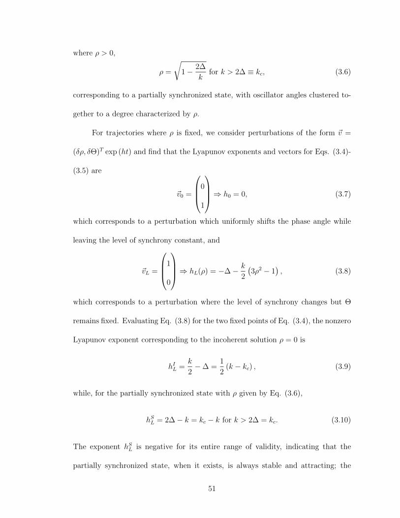
where ρ > 0,

ρ =

√1− 2∆

kfor k > 2∆ ≡ kc, (3.6)

corresponding to a partially synchronized state, with oscillator angles clustered to-

gether to a degree characterized by ρ.

For trajectories where ρ is fixed, we consider perturbations of the form ~v =

(δρ, δΘ)T exp (ht) and find that the Lyapunov exponents and vectors for Eqs. (3.4)-

(3.5) are

~v0 =

0

1

⇒ h0 = 0, (3.7)

which corresponds to a perturbation which uniformly shifts the phase angle while

leaving the level of synchrony constant, and

~vL =

1

0

⇒ hL(ρ) = −∆− k

2

(3ρ2 − 1

), (3.8)

which corresponds to a perturbation where the level of synchrony changes but Θ

remains fixed. Evaluating Eq. (3.8) for the two fixed points of Eq. (3.4), the nonzero

Lyapunov exponent corresponding to the incoherent solution ρ = 0 is

hIL =k

2−∆ =

1

2(k − kc) , (3.9)

while, for the partially synchronized state with ρ given by Eq. (3.6),

hSL = 2∆− k = kc − k for k > 2∆ = kc. (3.10)

The exponent hSL is negative for its entire range of validity, indicating that the

partially synchronized state, when it exists, is always stable and attracting; the

51

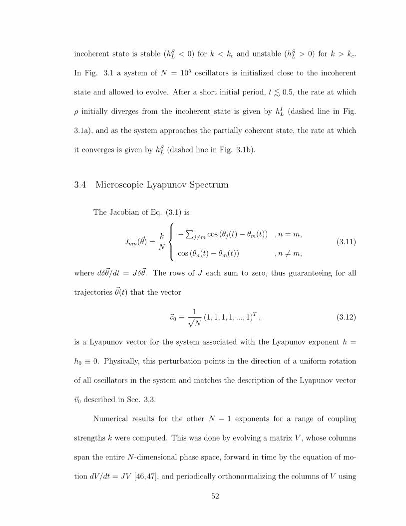
incoherent state is stable (hSL < 0) for k < kc and unstable (hSL > 0) for k > kc.

In Fig. 3.1 a system of N = 105 oscillators is initialized close to the incoherent

state and allowed to evolve. After a short initial period, t . 0.5, the rate at which

ρ initially diverges from the incoherent state is given by hIL (dashed line in Fig.

3.1a), and as the system approaches the partially coherent state, the rate at which

it converges is given by hSL (dashed line in Fig. 3.1b).

3.4 Microscopic Lyapunov Spectrum

The Jacobian of Eq. (3.1) is

Jmn(~θ) =k

N

−∑

j 6=m cos (θj(t)− θm(t)) , n = m,

cos (θn(t)− θm(t)) , n 6= m,

(3.11)

where dδ~θ/dt = Jδ~θ. The rows of J each sum to zero, thus guaranteeing for all

trajectories ~θ(t) that the vector

~v0 ≡1√N

(1, 1, 1, 1, ..., 1)T , (3.12)

is a Lyapunov vector for the system associated with the Lyapunov exponent h =

h0 ≡ 0. Physically, this perturbation points in the direction of a uniform rotation

of all oscillators in the system and matches the description of the Lyapunov vector

~v0 described in Sec. 3.3.

Numerical results for the other N − 1 exponents for a range of coupling

strengths k were computed. This was done by evolving a matrix V , whose columns

span the entire N -dimensional phase space, forward in time by the equation of mo-

tion dV/dt = JV [46,47], and periodically orthonormalizing the columns of V using

52

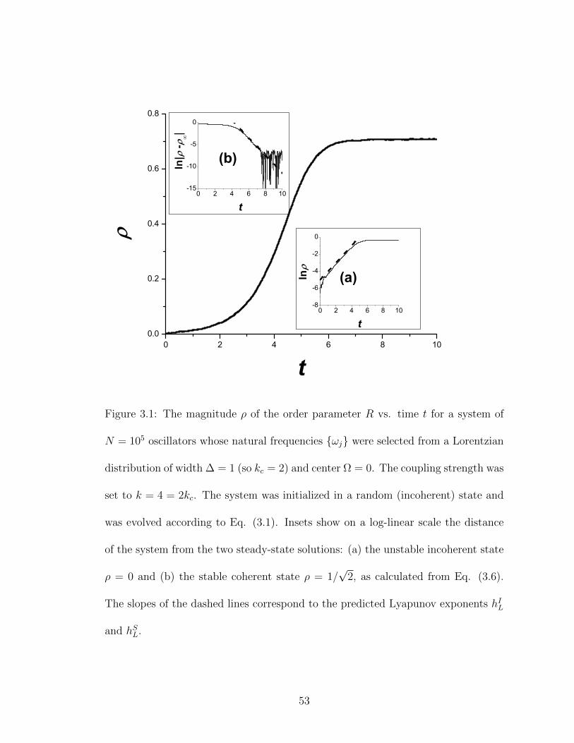
0 2 4 6 8 100.0

0.2

0.4

0.6

0.8

(b)

t

(a)

0 2 4 6 8 10-8

-6

-4

-2

0

ln

t

0 2 4 6 8 10-15

-10

-5

0

ln|

-|

t

Figure 3.1: The magnitude ρ of the order parameter R vs. time t for a system of

N = 105 oscillators whose natural frequencies ωj were selected from a Lorentzian

distribution of width ∆ = 1 (so kc = 2) and center Ω = 0. The coupling strength was

set to k = 4 = 2kc. The system was initialized in a random (incoherent) state and

was evolved according to Eq. (3.1). Insets show on a log-linear scale the distance

of the system from the two steady-state solutions: (a) the unstable incoherent state

ρ = 0 and (b) the stable coherent state ρ = 1/√

2, as calculated from Eq. (3.6).

The slopes of the dashed lines correspond to the predicted Lyapunov exponents hIL

and hSL.

53

the QR decomposition [48]. After a sufficiently long run time, the decomposition

of this matrix, V = QR, provides the Lyapunov exponents of the dynamics as the

diagonal elements of the upper-triangular matrix R, hn = Rnn, and the Lyapunov

vectors associated with each exponent as the columns of the orthonormalized matrix

Q (~vn is the nth column of Q).

Figure 3.2 plots these exponents for a particular random realization of the

natural frequencies, for k varied in the range 0 < k < 10, in a system of N =

200 oscillators. Tracing single Lyapunov exponents in Fig. 3.2 (solid curves) as

k is increased, we find that the exponents appear to have a common asymptotic

relation with k (except for the single exponent whose value is always zero and

whose associated direction is given by Eq. (3.12)). As k decreases, we find that

most exponents increase monotonically to near zero, at which point they remain

near zero for all k less than that value. The dependence of the nth largest exponent

hn as it approaches zero and the critical k value below which hn is near zero are

each different for different n. We will explore these properties further in Sec. 3.5.

3.4.1 Average Lyapunov Spectrum

Averaging over 2500 realizations (different initial conditions and selections for

ωj), Fig. 3.3 (dark colored curves) shows the distributions of Lyapunov exponents

in this spectrum for k = 1.0 < kc, k = 2.0 = kc, and two values for k > kc: k = 4

and k = 10. For k > kc the predominant features of these distributions is the

presence of two peaks: one peak centered around h = 0 and another peak centered

54

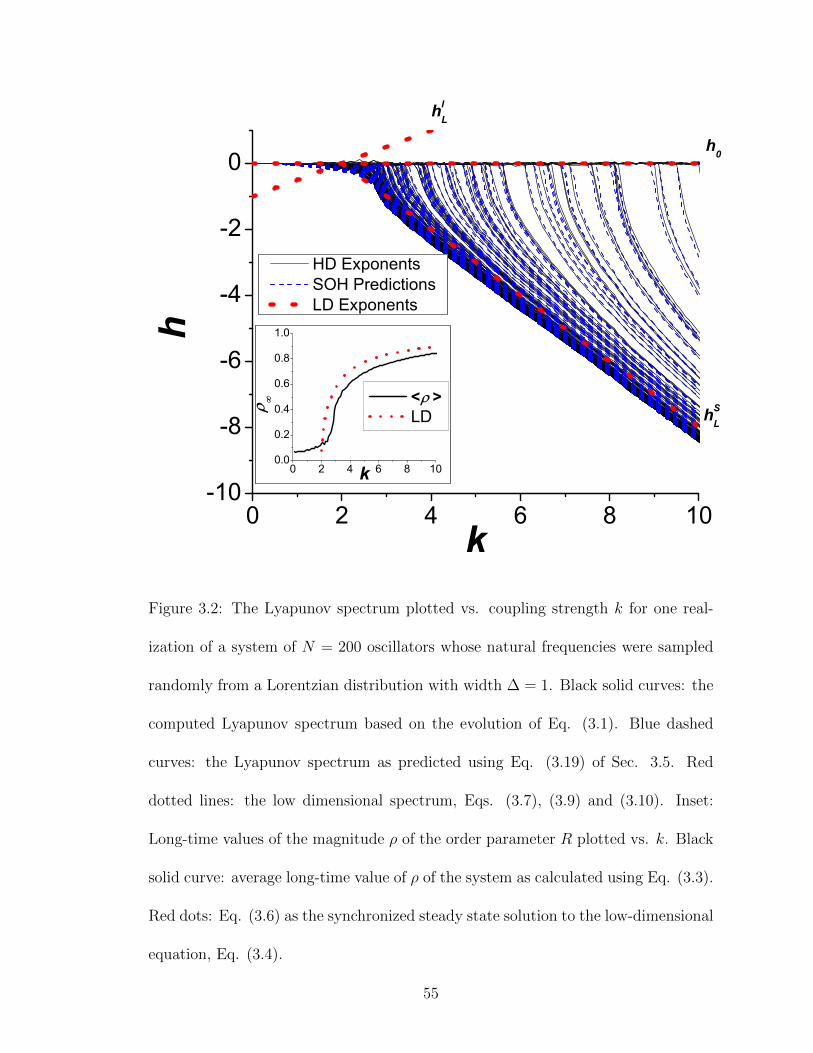
0 2 4 6 8 10-10

-8

-6

-4

-2

0

hIL

hSL

HD Exponents SOH Predictions LD Exponents

h

k

h0

0 2 4 6 8 100.0

0.2

0.4

0.6

0.8

1.0

< > LD

k

Figure 3.2: The Lyapunov spectrum plotted vs. coupling strength k for one real-

ization of a system of N = 200 oscillators whose natural frequencies were sampled

randomly from a Lorentzian distribution with width ∆ = 1. Black solid curves: the

computed Lyapunov spectrum based on the evolution of Eq. (3.1). Blue dashed

curves: the Lyapunov spectrum as predicted using Eq. (3.19) of Sec. 3.5. Red

dotted lines: the low dimensional spectrum, Eqs. (3.7), (3.9) and (3.10). Inset:

Long-time values of the magnitude ρ of the order parameter R plotted vs. k. Black

solid curve: average long-time value of ρ of the system as calculated using Eq. (3.3).

Red dots: Eq. (3.6) as the synchronized steady state solution to the low-dimensional

equation, Eq. (3.4).

55

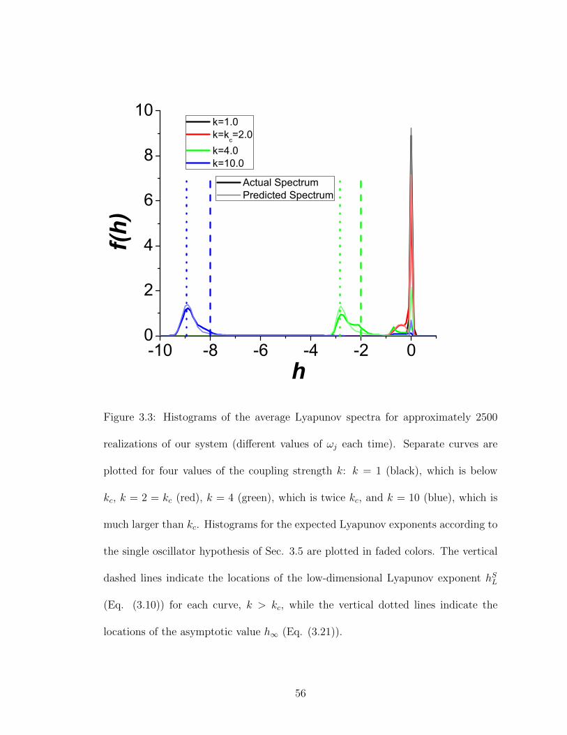
-10 -8 -6 -4 -2 00

2

4

6

8

10

Actual Spectrum Predicted Spectrum

f(h)

h

k=1.0 k=k

c=2.0

k=4.0 k=10.0

Figure 3.3: Histograms of the average Lyapunov spectra for approximately 2500

realizations of our system (different values of ωj each time). Separate curves are

plotted for four values of the coupling strength k: k = 1 (black), which is below

kc, k = 2 = kc (red), k = 4 (green), which is twice kc, and k = 10 (blue), which is

much larger than kc. Histograms for the expected Lyapunov exponents according to

the single oscillator hypothesis of Sec. 3.5 are plotted in faded colors. The vertical

dashed lines indicate the locations of the low-dimensional Lyapunov exponent hSL

(Eq. (3.10)) for each curve, k > kc, while the vertical dotted lines indicate the

locations of the asymptotic value h∞ (Eq. (3.21)).

56

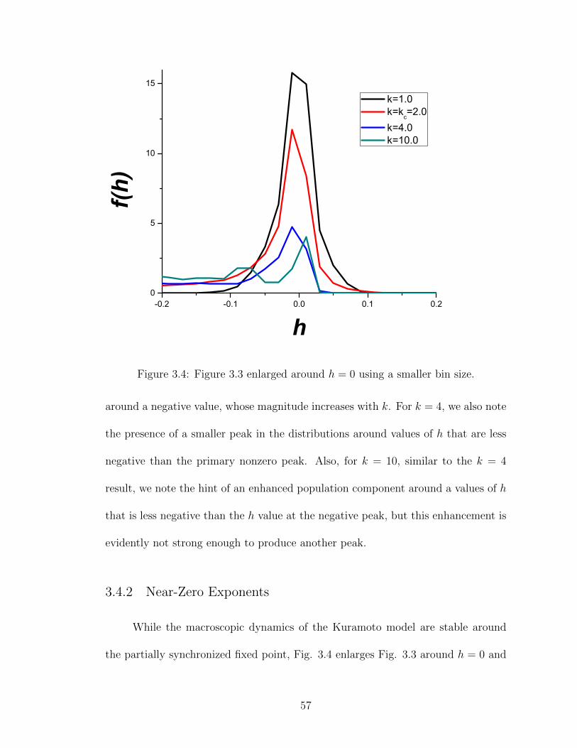
-0.2 -0.1 0.0 0.1 0.20

5

10

15

f(h)

h

k=1.0 k=k

c=2.0

k=4.0 k=10.0

Figure 3.4: Figure 3.3 enlarged around h = 0 using a smaller bin size.

around a negative value, whose magnitude increases with k. For k = 4, we also note

the presence of a smaller peak in the distributions around values of h that are less

negative than the primary nonzero peak. Also, for k = 10, similar to the k = 4

result, we note the hint of an enhanced population component around a values of h

that is less negative than the h value at the negative peak, but this enhancement is

evidently not strong enough to produce another peak.

3.4.2 Near-Zero Exponents

While the macroscopic dynamics of the Kuramoto model are stable around

the partially synchronized fixed point, Fig. 3.4 enlarges Fig. 3.3 around h = 0 and

57

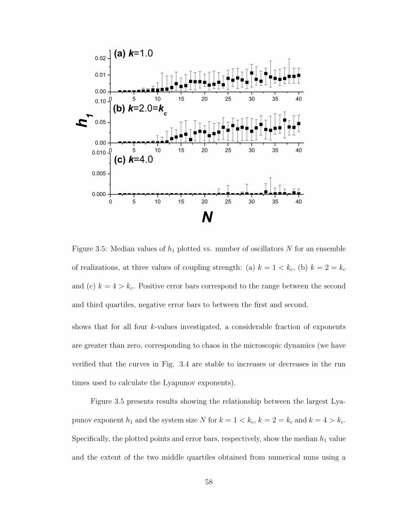
0 5 10 15 20 25 30 35 400.00

0.01

0.02

0 5 10 15 20 25 30 35 400.00

0.05

0.10

0 5 10 15 20 25 30 35 400.000

0.005

0.010

(b) k=2.0=kc

(a) k=1.0

(c) k=4.0

h 1

N

Figure 3.5: Median values of h1 plotted vs. number of oscillators N for an ensemble

of realizations, at three values of coupling strength: (a) k = 1 < kc, (b) k = 2 = kc

and (c) k = 4 > kc. Positive error bars correspond to the range between the second

and third quartiles, negative error bars to between the first and second.

shows that for all four k-values investigated, a considerable fraction of exponents

are greater than zero, corresponding to chaos in the microscopic dynamics (we have

verified that the curves in Fig. 3.4 are stable to increases or decreases in the run

times used to calculate the Lyapunov exponents).

Figure 3.5 presents results showing the relationship between the largest Lya-

punov exponent h1 and the system size N for k = 1 < kc, k = 2 = kc and k = 4 > kc.

Specifically, the plotted points and error bars, respectively, show the median h1 value

and the extent of the two middle quartiles obtained from numerical nuns using a

58

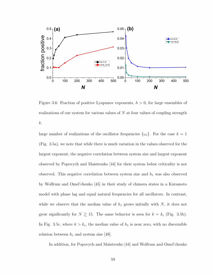
0 100 200 300 400 5000.0

0.1

0.2

0.3

0.4

0.5

0 100 200 300 400 5000.00

0.01

0.02

0.03

0.04

0.05 (b)

fract

ion

posi

tive

N

k=1.0 k=kc=2.0

(a)

N

k=4.0 k=10.0

Figure 3.6: Fraction of positive Lyapunov exponents, h > 0, for large ensembles of

realizations of our system for various values of N at four values of coupling strength

k.

large number of realizations of the oscillator frequencies ωi. For the case k = 1

(Fig. 3.5a), we note that while there is much variation in the values observed for the

largest exponent, the negative correlation between system size and largest exponent

observed by Popovych and Maistrenko [44] for their system below criticality is not

observed. This negative correlation between system size and h1 was also observed

by Wolfrum and Omel’chenko [45] in their study of chimera states in a Kuramoto

model with phase lag and equal natural frequencies for all oscillators. In contrast,

while we observe that the median value of h1 grows initially with N , it does not

grow significantly for N & 15. The same behavior is seen for k = kc (Fig. 3.5b).

In Fig. 3.5c, where k > kc, the median value of h1 is near zero, with no discernible

relation between h1 and system size [49].

In addition, for Popovych and Maistrenko [44] and Wolfrum and Omel’chenko

59

[45] each found for their systems that the proportion of Lyapunov exponents which

were positive was consistent as system size was varied, up to N = 80 for Popovych

and Maistrenko, and up to N = 50 for Wolfrum and Omel’chenko. In Fig. 3.6,

we show that the fraction of Lyapunov exponents observed to be positive over large

ensembles changed dramatically in the range N < 100: the fraction of positive

exponents increases with system size for k ≤ kc (Fig. 3.6a), leveling off only for

N & 200, and the fraction decreases with system size for k > kc (Fig. 3.6b), where

the fraction is constant for N & 100.

3.4.3 Comparison with Macroscopic Dynamics

While there is no a priori general reason to expect a precise correspondence

between the perturbation dynamics obtained from the microscopic and macroscopic

descriptions of a system, it is still of interest to compare them. As we have already

noted, an h0 corresponding to a uniform rotation of all the oscillator phases may be

obtained as an eigenvalue of the Jacobian for both the low dimensional system of

equations (Eqs. (3.4)-(3.5)) and the high dimensional system (Eq. (3.1)). As for hIL

given by Eq. (3.9), we observe for k < kc from Fig. 3.2 that it is substantially more

negative than the microscopic Lyapunov exponents (for k < kc), and the microscopic

and macroscopic Lyapunov numbers have qualitatively different behavior. However,

considering hSL for k > kc, given by Eq. (3.10), Fig. 3.2 shows that for large k, the

value of hSL scales with k at the same rate as the bulk of the microscopic spectrum.

On the other hand, in Fig. 3.3, we see that hSL is significantly less negative than the

60

bulk of the nonzero exponents.

To investigate further, we seek to characterize how “macroscopic” each high-

dimensional Lyapunov vector is. Given a perturbation δ~θ, we may linearize Eq.

(3.3) to find the effect such a perturbation on the complex order parameter:

δR =1

N

N∑j=1

eiθj iδθj. (3.13)

To compare the relative effect on R from perturbations in the directions of the Lya-

punov vectors, we will thus compare the magnitudes of the quantities∑N

j=1 eiθjvnj.

Using ~v0 given by Eq. (3.12) as a point of reference, we thus define the “macroscop-

icness” µn of a Lyapunov vector ~vn to be:

µn =|∑N

j=1 eiθjvnj|

|∑N

j=1 eiθjv0j|

=|∑N

j=1 eiθjvnj|

ρ√N

(3.14)

Figure 3.7 plots µn for each Lyapunov vector vs. its associated Lyapunov ex-

ponent for a single system of N = 500 oscillators at k = 4 > kc, showing that the

only significantly macroscopic perturbation of the system is the zero vector, with

the largest nontrivial µ having a value of only about 0.2. Additional numerical cal-

culations have shown this value to be a finite size effect, and (aside from the vector

~v0 with h = 0, µ ≡ 1) the largest µ varies roughly inversely with N . Furthermore,

we note the general trend that, as h becomes more negative, µ decreases, with the

least macroscopic vectors corresponding to the most negative Lyapunov exponent.

Together with Fig. 3.3, this leads to conclusion that the trend we observed between

hSL and the bulk of the microscopic Lyapunov exponents for large k is coinciden-

tal and that Lyapunov vectors with exponents around this value have no greater

connection to the macroscopic dynamics than any other vectors.

61

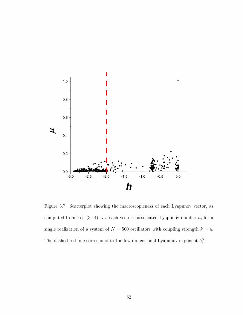
-3.0 -2.5 -2.0 -1.5 -1.0 -0.5 0.00.0

0.2

0.4

0.6

0.8

1.0

h

Figure 3.7: Scatterplot showing the macroscopicness of each Lyapunov vector, as

computed from Eq. (3.14), vs. each vector’s associated Lyapunov number hi for a

single realization of a system of N = 500 oscillators with coupling strength k = 4.

The dashed red line correspond to the low dimensional Lyapunov exponent hSL.

62

3.5 Single Oscillator Approximation of Lyapunov Vectors and Expo-

nents Based on the Behavior in the Mean Field

Equation (3.1) may be rewritten as

dθj(t)

dt= ωj + kρ(t) sin (Θ(t)− θj(t)) . (3.15)

From Eqs. (3.4)-(3.5), we expect that at long times, ρ will be fixed and Θ will vary

with a constant rate. Thus, seeking values of θj for which

Ω =dΘ

dt=dθjdt

= ωj + kρ sin (Θ− θj) . (3.16)

We call oscillators for which kρ > |ωj − Ω| “locked,” and these oscillators have

solutions to Eq. (3.16) given by

θ0j = sin−1

(ωj − Ω

kρ

)+ Θ (3.17)

while “unlocked” oscillators have θj(t) either increasing or decreasing monotonically

with time at a constant average rate. We now show that, for N >> 1, most of the

Lyapunov exponents correspond to perturbations of single oscillators forced by the

mean field and represented by the Lyapunov vectors ~vSOHj with one entry of unity

and the rest zero:

~vSOHj = (δ1j, δ2j, δ3j, δ4j, ..., δNj)T . (3.18)

Figures 3.8(a,b) show, via greyscale heat maps, the extent to which these pre-

dicted Lyapunov vectors match the actual Lyapunov vectors of the system. The

vertical and horizontal axes are indices n of Lyapunov vectors ordered so that

63

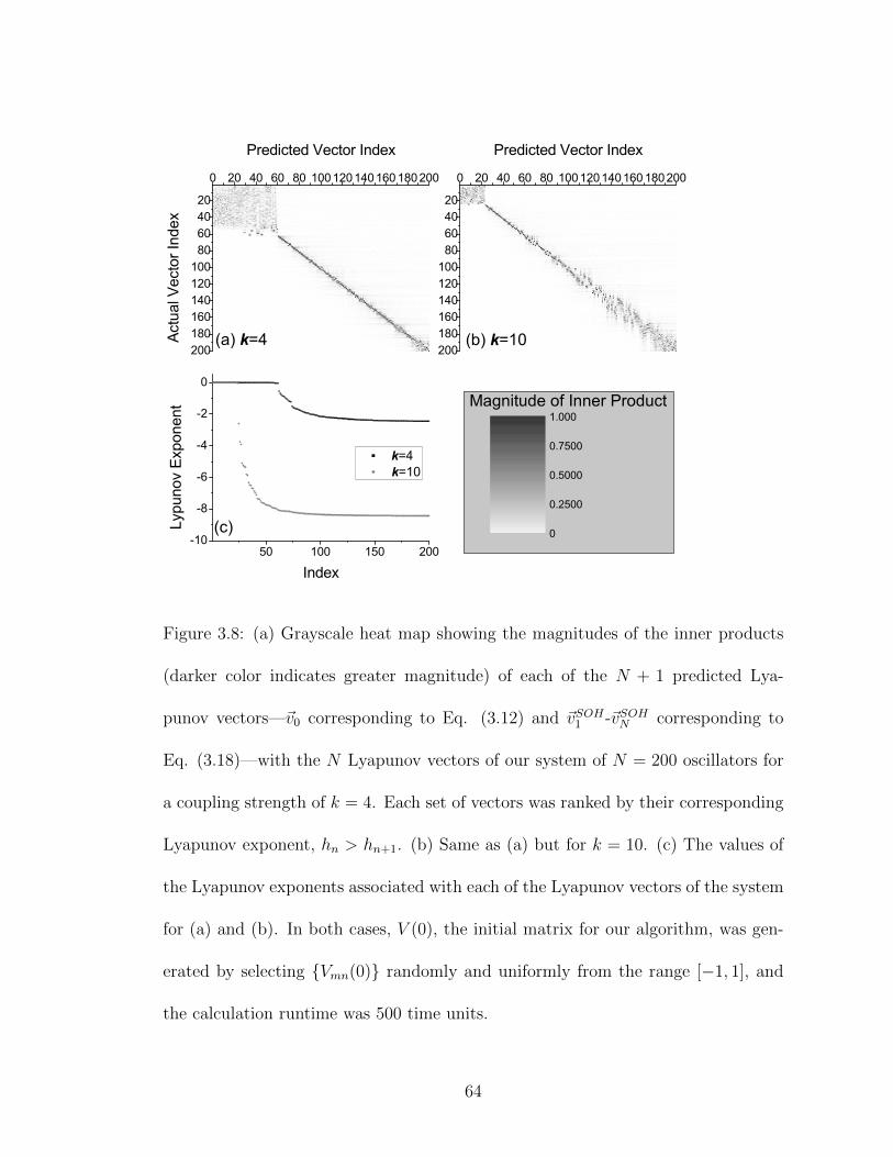
50 100 150 200-10

-8

-6

-4

-2

0

0 20 40 60 80 100120140160180200

20406080

100120140160180200

Actu

al V

ecto

r Ind

exPredicted Vector Index

0

0.2500

0.5000

0.7500

1.000

0 20 40 60 80 100120140160180200

20406080

100120140160180200

Predicted Vector Index

Magnitude of Inner Product

(c)

(b) k=10

k=4 k=10

Lypu

nov

Expo

nent

Index

(a) k=4

Figure 3.8: (a) Grayscale heat map showing the magnitudes of the inner products

(darker color indicates greater magnitude) of each of the N + 1 predicted Lya-

punov vectors—~v0 corresponding to Eq. (3.12) and ~vSOH1 -~vSOHN corresponding to

Eq. (3.18)—with the N Lyapunov vectors of our system of N = 200 oscillators for

a coupling strength of k = 4. Each set of vectors was ranked by their corresponding

Lyapunov exponent, hn > hn+1. (b) Same as (a) but for k = 10. (c) The values of

the Lyapunov exponents associated with each of the Lyapunov vectors of the system

for (a) and (b). In both cases, V (0), the initial matrix for our algorithm, was gen-

erated by selecting Vmn(0) randomly and uniformly from the range [−1, 1], and

the calculation runtime was 500 time units.

64

hn > hn+1, where the hn’s for the vertical scale are from our previously described

computations of the Lyapunov spectrum of Eq. (3.1), and the hn’s for the horizontal

scale are obtained from the single oscillator hypothesis (Eq. (3.19)). In both cases

plotted in Figs. 3.8(a,b), k = 4 and k = 10, a proportion of the corresponding

Lyapunov exponents (plotted in Fig. 3.8(c)) are near zero, and thus that part of

the spectra is nearly degenerate. Consequently, the upper-left corners of the Fig.

3.8(a,b) are blocks of seemingly random values. In addition, as seen best in Fig.

3.8(b), the bottom-right corner is somewhat degenerate as well, due to the fact that

the most negative Lyapunov exponents have values that are very close to each other

as they approach their predicted common asymptotic value observed in Fig. 3.2.

In between, however, most of the actual Lyapunov vectors agree well with their

corresponding predicted Lyapunov vector ~vSOHj . The lack of perfect agreement is

probably due, at least partially, to the fact that the single oscillator hypothesis pro-

vides only an approximate solution to the dynamics, since, although N >> 1, it is

still finite. That being said, we believe that some of the discrepancy observed may

also be due to numerical limitations of the algorithm—to differentiate between the

nearly degenerate most-negative Lyapunov exponents, our algorithm would have to

be run for an extremely long time [50].

Linearizing Eq. (3.15) with respect to θj and evaluating at θ0j we obtain a

prediction for the Lyapunov exponent of a locked state oscillator j,

hSOHj ' −√k2ρ2 − (ωj − Ω)2 , kρ > |ωj − Ω|. (3.19)

Again we note that this is an approximate equation which ignores the finite-N noisy

65

fluctuations of ρ and Θ. For kρ < |ωj − Ω|, Eq. (3.16) has no solution. In that

case, θj −Θ will be monotonically increasing or decreasing, and since Eq. (3.16) is

one-dimensional, the Lyapunov exponent in that case will be

hSOHj = 0 for kρ < |ωj − Ω|. (3.20)

The Lyapunov spectrum as predicted by the single oscillator hypothesis was

also plotted in Fig. 3.2 (dashed blue curves) and in 3.3 (faded color curves), showing

that the majority of exponents are well predicted by the single oscillator hypothesis.

The values hj(k) agree well with those predicted by Eqs. (3.19)-(3.20), and the

critical values of k below which hi ' 0 are given by |ωj −Ω|/ρ. We also find that it

is the single oscillator hypothesis, not the low dimensional theory, that gives us the

asymptotic value for hi for large k: Inserting the value of ρ given by by Eq. (3.6)

into Eq. (3.19), we find the asymptotic value of hj in the limit kρ >> |ωj − Ω|:

h∞ =√k(kc − k). (3.21)

Figure 3.3 showed h∞ as a dotted vertical line, showing that the main nonzero

peak for the distributions of Lyapunov exponents is centered around this value h∞.

The width of this peak is a finite size effect, and as the number of oscillators is

increased, this peak becomes narrower. This is reflected by comparing Fig. 3.3

and Fig. 3.9, which shows the distribution of Lyapunov exponents for a system of

N = 500 oscillators.

As a final demonstration, Fig. 3.10 applies the single oscillator hypothesis to

the analysis of a system where the natural frequency distribution is Gaussian in

form rather than Lorentzian. As expected, the hypothesis does just as well in this

66

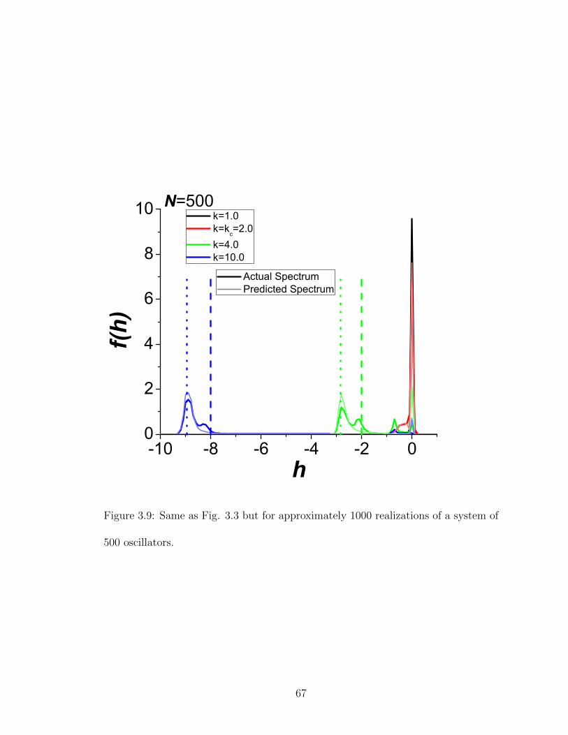
-10 -8 -6 -4 -2 00

2

4

6

8

10 N=500

Actual Spectrum Predicted Spectrum

f(h)

h

k=1.0 k=k

c=2.0

k=4.0 k=10.0

Figure 3.9: Same as Fig. 3.3 but for approximately 1000 realizations of a system of

500 oscillators.

67

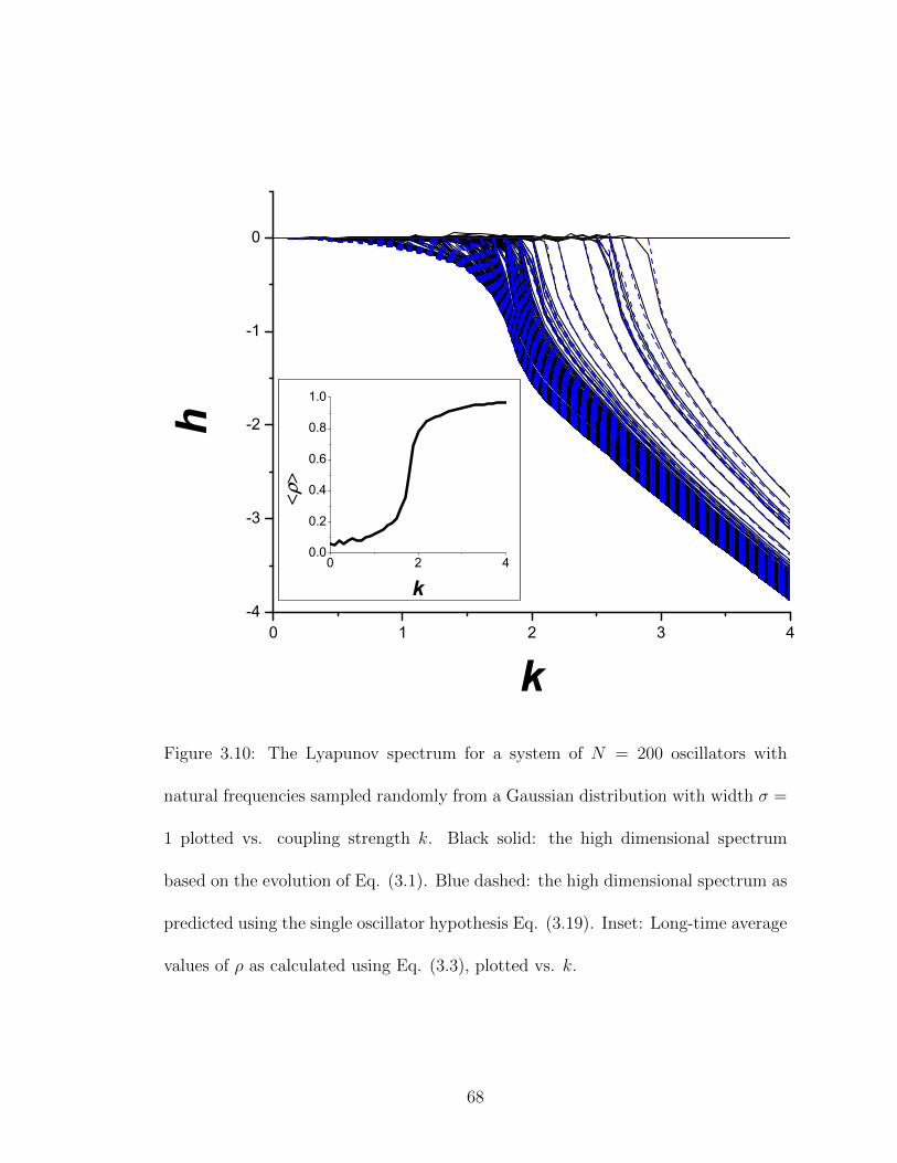
0 1 2 3 4-4

-3

-2

-1

0

h

k

0 2 40.0

0.2

0.4

0.6

0.8

1.0

k

Figure 3.10: The Lyapunov spectrum for a system of N = 200 oscillators with

natural frequencies sampled randomly from a Gaussian distribution with width σ =

1 plotted vs. coupling strength k. Black solid: the high dimensional spectrum

based on the evolution of Eq. (3.1). Blue dashed: the high dimensional spectrum as

predicted using the single oscillator hypothesis Eq. (3.19). Inset: Long-time average

values of ρ as calculated using Eq. (3.3), plotted vs. k.

68

case as for the Lorentzian, Eq. (3.2), predicting the critical values of k below which

hj is near zero, the asymptotic behavior for kρ >> |ωj − ω| (where ω is the center

of the Gaussian distribution) and the intermediate values hj(k).

3.6 Conclusion

We summarize our conclusions as follows:

(i) For large N and k > kc, Lyapunov exponents with appreciably negative values

can be well approximated as resulting from specific individual “locked oscilla-

tors” (i.e., oscillators with |ωj| < kρ) that are forced by the mean field. The

complementary nonlocked oscillators contribute a spectral component of Lya-

punov exponents with values near zero, some of which are slightly negative

and some slightly positive (corresponding to chaotic dynamics). These latter

oscillators are smaller in number for larger k/kc, and we show how the number

of positive exponents scales with N and k.

(ii) We believe that our finding in (i) (that many of the Lyapunov exponents

in the spectrum can be well described by examination of the perturbation

dynamics of individual oscillators forced by the mean field) should have general

applicability to many large systems of heterogeneous dynamical units that are

coupled by a mean field.

(iii) Chaos of the finite N system as characterized by the largest Lyapunov expo-

nent h1 has been found to be approximately independent of the system size N .

This finding contrasts with the N−1 scaling of h1 found in Refs. [44,45] which

69

investigate somewhat different situations. Thus it appears that the scaling of

h1 with N can be different under different circumstances, and that universality

in the saling of h1 with N is unlikely.

70

Chapter 4: The Stability of Adaptive Synchronization

of Chaotic Systems

4.1 Overview

We consider an adaptive scheme for maintaining the synchronized state in a

network of identical coupled chaotic systems in the presence of a priori unknown

slow temporal drift in the couplings. Stability of this scheme is addressed through

an extension of the master stability function technique to include adaptation. We

observe that noise and/or slight nonidenticality between the coupled systems can

be responsible for the occurrence of intermittent bursts of large desynchronization

events (bubbling). Moreover, our numerical computations show that, for our adap-

tive synchronization scheme, the parameter space region corresponding to bubbling

can be rather substantial. This observation becomes important to experimental

realizations of adaptive synchronization, in which small mismatches in the parame-

ters and noise cannot be avoided. We also find that, for our coupled systems with

adaptation, bubbling can be caused by a slow drift in the coupling strength.

71

4.2 Introduction

It has been shown [37, 38, 51] that, in spite of their random-like behavior, the

states xi(t) (i = 1, 2, ..., N) of a collection of N interacting chaotic systems that

are identical can synchronize (i.e., be attracted toward a common chaotic evolution,

x1(t) = x2(t) = ... = xN(t)) provided that they are properly coupled. This phe-

nomenon has been the basis for proposals for secure communication [52–54], system

identification [55–58], data assimilation [59, 60], sensors [61], information encoding

and transmission [62,63], multiplexing [64], combatting channel distortion [65], etc.

In all of these applications it is typically assumed that one has accurate knowledge

of the interaction between the systems, allowing one to choose the appropriate cou-

pling protocol at each node (here we use the network terminology, referring to the

N chaotic systems as N nodes of a connected network whose links (i, j) correspond

to the input that node i receives from node j). In a recent paper [66], an adaptive

strategy was proposed for maintaining synchronization between identical coupled

chaotic dynamical systems in the presence of a priori unknown, slowly time vary-

ing coupling strengths (e.g., as might arise from temporal drift of environmental

parameters). This strategy was successfully tested on computer simulated networks

of many coupled dynamical systems in which, at each time, every node receives

only one aggregate signal representing the superposition of signals transmitted to it

from the other network nodes. In addition, the strategy has also been successfully

implemented in an experiment on coupled optoelectronic feedback loops [67]. Fur-

thermore, a more generalized adaptive strategy, suitable for sensor applications, has

72

also been proposed [61].

In past works, various other schemes for adaptive synchronization of chaos

have also been proposed [68–77]. So far, in all these studies, when the question

of stability of the considered adaptive schemes has been studied, the question has

been addressed using the Lyapunov function method (see e.g., [70,71,73,75]), which

provides a sufficient but not necessary condition for stability. While this technique

has the advantage that it can sometimes yield global stability conditions, it also has

the disadvantages that its applicability is limited to special cases, and its implemen-

tation, when possible, requires nontrivial system specific analysis. In this chapter,

we address the stability of adaptive synchronization for the example of the scheme

discussed in Ref. [66]. In particular, our analysis will extend the previously de-

veloped stability analysis of chaos synchronization by the master stability function

technique [37, 38] to include adaptation. We will observe that the range in which

the network eigenvalues are associated with stability, is dependent on the choice

of the parameters of the adaptive strategy. The type of analysis we present, while

for a specific illustrative adaptive scheme, can be readily applied to other adaptive

schemes (e.g., those in [76,77]).

As compared to the Lyapunov technique, master stability techniques are much

more generally applicable but they provide conditions for local, rather than global

stability. We also note that, within that context, the master stability technique

allows one to distinguish between stability of typical chaotic orbits and stability of

atypical orbits within the synchronizing chaotic attractor (i.e., stability to ‘bubbling’

[6, 78–80,82,83]; see Secs. 4.4 and 4.5).

73

In Sec. 4.3 we review the adaptive synchronization strategy formulation of

Ref. [66], which applies to a network of chaotic systems with unknown temporal

drifts of the couplings. In Sec. 4.4, we present a master stability function approach

to study linear stability of the synchronized solution in the presence of adaptation;

we also consider a generalized formulation of our adaptive strategy and study its

stability. Numerical simulations are finally presented in Sec. 4.5. Our work in Sec.

4.5 highlights the important effect of bubbling in the dynamics.

4.3 Adaptive strategy formulation

As our example of the application of the master stability technique to an adap-

tive scheme, we consider the particular scheme presented in Ref. [66]. To provide

background, in this section we present a brief exposition of a formulation similar to

that in Ref. [66], as motivated by the situation where the couplings are unknown

and drift with time. We consider a situation where the dynamics at each of the

network nodes is described by,

xi(t) = F (xi(t)) + γΓ[σi(t)ri(t)−H(xi(t))], i = 1, ..., N, (4.1)

where, xi is the m-dimensional state of system i = 1, ..., N ; F (x) determines the

dynamics of an uncoupled (γ → 0) system (hereafter assumed chaotic), F : Rm →

Rm; H(x) is a scalar output function, H : Rm → R. We take Γ to be a constant

m-vector, Γ = [Γ1,Γ2, ...,Γm]T , with∑

i Γ2i = 1, and the scalar γ is a constant

characterizing the strength of the coupling. The scalar signal each node i receives

74

from the other nodes in the network is,

ri(t) =∑j

Aij(t)H(xj(t)). (4.2)

The quantity Aij(t) is an adjacency matrix whose values specify the strengths of the

couplings from node j to node i. We note that if

σi(t) = [∑j

Aij]−1 (4.3)

then Eq. (4.1) admits a synchronized solution,

x1(t) = x2(t) = ... = xN(t) = xs(t), (4.4)

where xs(t) satisfies

xs(t) = F (xs(t)), (4.5)

which corresponds to the dynamics of an isolated system. We regard the Aij(t) as

unknown at each node i, while the only external information available at node i is

its received signal (4.2). The goal of the adaptive strategy is to adjust σi(t) so as to

maintain synchronism in the presence of slow, a priori unknown time variations of

the quantities Aij(t). That is, we wish to maintain approximate satisfaction of Eq.

(4.3). For this purpose, as discussed in Ref. [66], our scheme can be extended to the

case where the output function is `-dimensional, H : Rm → R`, where ` < m and Γ

is an `×m dimensional matrix. For simplicity we consider ` = 1. We assume that

each node independently implements an adaptive strategy. At each system node i,

we define the exponentially weighted synchronization error ψi = 〈(σiri −H(xi))2〉ν ,

where

〈G(t)〉ν =

∫ t

G(t′)e−ν(t′−t)dt′, (4.6)

75

and we evolve σi(t) so as to minimize this error (a slightly more general approach

is taken in [66]). We then set ∂ψi/∂σi equal to zero to obtain

σi(t) =〈H(xi(t))ri(t)〉ν〈ri(t)2〉ν

=pi(t)

qi(t). (4.7)

By virtue of d 〈G(t)〉ν/dt = −ν 〈G(t)〉ν + G(t), we obtain the numerator and the

denominator on the right-hand side of Eq. (4.7) by solving the differential equations,

pi(t) = −νpi(t) + ri(t)H(xi(t)), (4.8a)

qi(t) = −νqi(t) + ri(t)2. (4.8b)

Since we imagine the dynamics of Aij(t) occur on a timescale which is slow compared

to the other dynamics in the network, we can approximate Aij(t) as constant Aij.

This essentially assumes that we are dealing with perturbations from synchroniza-

tion whose growth rates (in the case of unstable synchronization) or damping rates

(in the case of stable synchronization) have magnitudes that substantially exceed

|A−1ij (t)dAij/dt|. Under this assumption, we note that Eqs. (4.1), (4.7), and (4.8)

admit a synchronized solution, given by Eqs. (4.4), (4.5), and

psi = −νpsi + (∑j

Aij)H(xs)2, i = 1, ..., N, (4.9a)

qsi = −νqsi + (∑j

Aij)2H(xs)2, i = 1, ..., N. (4.9b)

To simplify the notation, in what follows, we take DF s(t) = DF (xs(t)), Hs(t) =

H(xs(t)), and DHs(t) = DH(xs(t)); e.g., we can now write,

psi = ki⟨(Hs)2

⟩ν,

qsi = k2i

⟨(Hs)2

⟩ν,

(4.10)

76

where ki = (∑

j Aij). If the synchronization scheme is locally stable, we expect that

the synchronized solution Eqs. (4.4), (4.5) and (4.9) will be maintained under slow

time evolution of the couplings Aij(t).

4.4 Stability analysis

4.4.1 Linearization and master stability function

Our goal is to study the stability of the reference solution Eqs. (4.4), (4.5) and

(4.9). By linearizing Eqs. (4.1) and (4.8) about Eqs. (4.5), and (4.9), we obtain,

δxi = DF sδxi + γΓ

DHs

[k−1i

∑j

Aijδxj − δxi]+

Hs

k2i 〈(Hs)2〉ν

εi

, i = 1, ..., N,

(4.11a)

εi = −νεi −HsDHski

[∑j

Aijδxj − kiδxi], i = 1, ..., N,

(4.11b)

where we have introduced the new variable εi(t) = kiδpi(t)− δqi(t).

Equations (4.11) constitute a system of (m+ 1)N coupled equations. In order

to simplify the analysis, we seek to decouple this system into N independent systems,

each of dimension (m + 1). For this purpose we seek a solution where δxi is in the

form δxi = cix(t), where ci is a time independent scalar that depends on i and x(t) is

a m-vector that depends on time but not on i. Substituting in Eqs. (4.11a),(4.11b),

77

we obtain,

˙x = DF sx+ γΓ

[∑j Aijcj

kici− 1

]DHsx+

γΓHs

cik2i 〈(Hs)2〉ν

εi, i = 1, ..., N, (4.12a)

εi = −νεi − ki[∑

j

Aijcj − kici]HsDHsx, i = 1, ..., N. (4.12b)

To make Eqs. (4.12) independent of i, we consider β(t) = εi(t)/[ciki2(α − 1)] and∑

j Aijcj = αkici, where α is a quantity independent of i. Namely, the possible

values of α are the eigenvalues, A′~c = α~c, corresponding to linearly independent

eigenvectors ~c = [c1, c2, ..., cN ]T , where A′ = A′ij = ki−1Aij. This gives,

˙x = DF sx− γ(1− α)

[ΓDHsx+ Γ

Hsβ

〈(Hs)2〉ν

], (4.13a)

β = −νβ −HsDHsx, (4.13b)

which is independent of i, but depends on the eigenvalue α. Considering the typ-

ical case where there are N distinct eigenvalues of the N × N matrix A′, we see

that Eqs. (4.12) constitute N decoupled linear ordinary differential equations for

the synchronization perturbation variables x and β. All the rows of A′ sum to 1.

Therefore A′ has at least one eigenvalue α = 1, corresponding to the eigenvector

c1 = c2 = ... = cN = 1. Furthermore, since A′ij ≥ 0 for all (i, j), we have by the

Perron-Frobenius theorem that α ≤ 1, and thus (1−α) ≥ 0. For α = 1, Eq. (4.13a)

becomes,

˙x = DF sx. (4.14)

This equation reflects the chaos of the reference synchronized state (Eq. (4.5)) and

(because all the ci are equal) is associated with perturbations which are tangent to

the synchronization manifold and are therefore irrelevant in determining synchro-

78

nization stability. Stability of the synchronized state thus demands that Eqs. (4.12)

yield exponential decay of x and β for all the (N − 1) eigenvalues α, excluding this

α = 1 eigenvalue.

It thus becomes possible to introduce a master stability function [37,38], M(ξ),

that associates the maximum Lyapunov exponent of system (4.13) with ξ = γ(1−α).

In so doing, one decouples the effects of the network topology (reflected in the

eigenvalues α and hence the relevant values of ξ = γ(1 − α)) from the choices of

F,H, ν. In general an eigenvalue, and hence also ξ, can be complex. For simplicity,

in our discussion and numerical examples to follow, we assume that the eigenvalues

are real (which is for instance the case when the adjacency matrix is symmetric).

For any given value of γ stability demands that M(ξ) < 0 for all those values of

ξ = γ(1− α) corresponding to the eigenvalues α 6= 1.

Following Refs. [84–87], we now introduce the following definition of synchro-

nizability. Let us assume that the master stability function M(ξ) is negative in

a bounded interval of values of ξ, say [ξ−, ξ+]. Then, in order for the network to

synchronize, two conditions need to be satisfied, (i) ξ− < γ(1 − αmin), and (ii)

ξ+ > γ(1 − αmax), where αmin (αmax) is the smallest (largest) network eigenvalue

over all the eigenvalues α 6= 1. The network synchronizability is defined as the width

of the range of values of γ, for which M(ξ) < 0. Assuming that αmin and αmax are

assigned (e.g., the network topology is given), then the network synchronizability

increases with the ratio ξ+/ξ−. In what follows, we will compare different adaptive

strategies in terms of their effects on the synchronizability ratio ξ+/ξ−.

In our analysis above, since we divide by ki, we have implicitly assumed that

79

all the ki 6= 0, i.e., that every node has an input. There is, however, a case of interest

where this is not so, and this case requires separate consideration. In particular, say

there is one and only one special node (which we refer to as the maestro or sender)

that has no inputs, but sends its output to other nodes (which interact with each

other), and we give this special node the label i = N . Since node N receives no

inputs, we do not include adaption on this node, and we replace Eq.(1) for i = N by

xN(t) = F (xN(t)). In addition, when investigating the stability of the synchronized

state, it suffices to set δxN(t) = 0 (i.e., not to perturb the maestro). Following the

steps of our previous stability analysis, we again obtain Eqs. (4.12) and (4.13), but

with important differences. Namely, Eqs. (4.12) now apply for i = 1, ..., N − 1, the

values of α in Eqs. (4.13) are now the eigenvalues of the (N − 1)× (N − 1) matrix

A′ij = ki−1Aij for i, j = 1, 2, ..., (N − 1); i.e., only the interactions between the

nodes i, j ≤ (N − 1) are included in this matrix. Note that ki is still given by∑Nj=1Aij, still including the input AiN from the maestro node. Also since δxN = 0,

all of the eigenvalues represent transverse perturbations and are therefore relevant

to stability. (This is in contrast to the case without a maestro in which we had to

exclude an eigenvalue, i.e., α = 1 corresponding to c1 = c2 = ... = cN = 1. For

a similar discussion for the case of the standard master stability problem with no

adaptation, see [88].) The simplest case of this type (used in some of our subsequent

numerical experiments) is the case N = 2, where there is one receiver node (i = 1)

and one sender/maestro node (i = 2). Since there is only one receiver node whose

only input is received by the sender, A reduces to the scalar A = 0 and α = 0,

yielding ξ ≡ γ.

80

As stated above, xs(t) in (4.4) is an orbit of the uncoupled system (4.4). In

general, two types of orbits xs(t) are of interest: (i) a typical chaotic orbit on

the relevant chaotic attractor of (4.4), and (ii) the orbit that is ergodic on the

maximally synchronization-unstable invariant subset embedded within the relevant

chaotic attractor of (4.4). Here, by ‘relevant chaotic attractor’ we mean that, if the

system (4.4) has more than one attractor, then we restrict attention to that attractor

on which synchronized motion is of interest. Also, in (i), by the word ‘typical’, we

mean orbits of (4.4) that ergodically generate the measure that applies for Lebesgue

almost every initial condition in the attractor’s basin of attraction. In this sense,

the orbit in (ii) is not typical. In general the criterion for stability as assessed by (ii)

is more restrictive than that assessed by (i). Conditions in which the synchronized

dynamics is stable according to (i), but unstable according to (ii), are referred

to as the ‘bubbling’ regime [6, 78–80, 82]. In previous work on synchronization of

chaos [6, 78–80, 82, 83], it has been shown that, when the system is in the bubbling

regime, small noise and/or small ‘mismatch’ between the coupled systems can lead

to rare, intermittent, large deviations from synchronism, called ‘desynchronization

bursts’ [81]. By small system mismatch we mean that, for each node i, the functions

F in (4.1) are actually different, F → Fi, but that these differences are small

(i.e., |Fi(x)−F (x)| is small, where F (x) now denotes a reference uncoupled system

dynamics; e.g., Fi averaged over i). With reference to our adaptive synchronization

problem (4.1), we shall see that, in addition to small noise and small mismatch

in F , bursting can also be induced by slow drift in the unknown couplings Aij(t).

From the practical, numerical perspective, the complete and rigorous application

81

of the stability criterion (ii) is impossible, since there will typically be an infinite

number of distinct invariant sets embedded in a chaotic attractor, and, to truly be

sure of stability, each of these must be found and numerically tested. In practice,

therefore, as done previously by others, we will evaluate stability for all the unstable

periodic orbits embedded in the attractor up to some specified period. This will give

a necessary condition for stability according to (ii), and furthermore, it has been

argued and numerically verified in Ref. [82] that stability, as assessed from a large

collection of low period periodic orbits (and embedded unstable fixed points, if they

exist in the relevant attractor), will extremely often yield the true delineation of the

parameters of the bubbling regime, or, if not, an accurate approximation of it. Our

numerical results of Sec. IV lend further support to this idea.

4.4.2 Generalized adaptive strategy

We now analyze a generalization of our adaptive strategy. Namely, we replace

Eq. (4.8b) by,

pi(t) = −νpi(t) + [qi(t)/pi(t)]H(xi(t))2Q

(pi(t)ri(t)

qi(t)H(xi(t))

), (4.15)

where Q(z) is an arbitrary function of z, normalized so that Q(1) ≡ 1. The key

point is that at synchronism σiri = H(xi(t)), corresponding to piri = qiH(xi(t));

and thus, since we take Q(1) = 1, the synchronized solution is unchanged. The

stability analysis for this generalization is given in the Appendix I and results in the

82

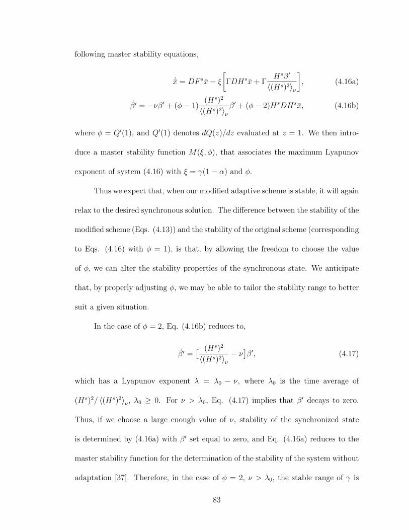
following master stability equations,

˙x = DF sx− ξ[ΓDHsx+ Γ

Hsβ′

〈(Hs)2〉ν

], (4.16a)

β′ = −νβ′ + (φ− 1)(Hs)2

〈(Hs)2〉νβ′ + (φ− 2)HsDHsx, (4.16b)

where φ = Q′(1), and Q′(1) denotes dQ(z)/dz evaluated at z = 1. We then intro-

duce a master stability function M(ξ, φ), that associates the maximum Lyapunov

exponent of system (4.16) with ξ = γ(1− α) and φ.

Thus we expect that, when our modified adaptive scheme is stable, it will again

relax to the desired synchronous solution. The difference between the stability of the

modified scheme (Eqs. (4.13)) and the stability of the original scheme (corresponding

to Eqs. (4.16) with φ = 1), is that, by allowing the freedom to choose the value

of φ, we can alter the stability properties of the synchronous state. We anticipate

that, by properly adjusting φ, we may be able to tailor the stability range to better

suit a given situation.

In the case of φ = 2, Eq. (4.16b) reduces to,

β′ =[ (Hs)2

〈(Hs)2〉ν− ν]β′, (4.17)

which has a Lyapunov exponent λ = λ0 − ν, where λ0 is the time average of

(Hs)2/ 〈(Hs)2〉ν , λ0 ≥ 0. For ν > λ0, Eq. (4.17) implies that β′ decays to zero.

Thus, if we choose a large enough value of ν, stability of the synchronized state

is determined by (4.16a) with β′ set equal to zero, and Eq. (4.16a) reduces to the

master stability function for the determination of the stability of the system without

adaptation [37]. Therefore, in the case of φ = 2, ν > λ0, the stable range of γ is

83

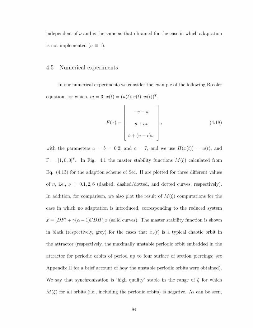
independent of ν and is the same as that obtained for the case in which adaptation

is not implemented (σ ≡ 1).

4.5 Numerical experiments

In our numerical experiments we consider the example of the following Rossler

equation, for which, m = 3, x(t) = (u(t), v(t), w(t))T ,

F (x) =

−v − w

u+ av

b+ (u− c)w

, (4.18)

with the parameters a = b = 0.2, and c = 7, and we use H(x(t)) = u(t), and

Γ = [1, 0, 0]T . In Fig. 4.1 the master stability functions M(ξ) calculated from

Eq. (4.13) for the adaption scheme of Sec. II are plotted for three different values

of ν, i.e., ν = 0.1, 2, 6 (dashed, dashed/dotted, and dotted curves, respectively).

In addition, for comparison, we also plot the result of M(ξ) computations for the

case in which no adaptation is introduced, corresponding to the reduced system

˙x = [DF s + γ(α− 1)ΓDHs]x (solid curves). The master stability function is shown

in black (respectively, grey) for the cases that xs(t) is a typical chaotic orbit in

the attractor (respectively, the maximally unstable periodic orbit embedded in the

attractor for periodic orbits of period up to four surface of section piercings; see

Appendix II for a brief account of how the unstable periodic orbits were obtained).

We say that synchronization is ‘high quality’ stable in the range of ξ for which

M(ξ) for all orbits (i.e., including the periodic orbits) is negative. As can be seen,

84

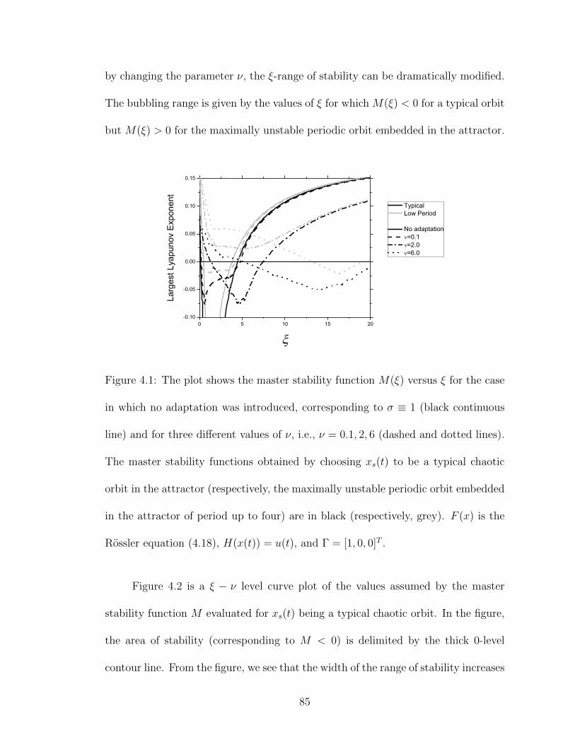
by changing the parameter ν, the ξ-range of stability can be dramatically modified.

The bubbling range is given by the values of ξ for which M(ξ) < 0 for a typical orbit

but M(ξ) > 0 for the maximally unstable periodic orbit embedded in the attractor.

0 5 10 15 20-0.10

-0.05

0.00

0.05

0.10

0.15

La

rges

t Lya

puno

v E

xpon

ent

Typical Low Period

No adaptation =0.1 =2.0 =6.0

Figure 4.1: The plot shows the master stability function M(ξ) versus ξ for the case

in which no adaptation was introduced, corresponding to σ ≡ 1 (black continuous

line) and for three different values of ν, i.e., ν = 0.1, 2, 6 (dashed and dotted lines).

The master stability functions obtained by choosing xs(t) to be a typical chaotic

orbit in the attractor (respectively, the maximally unstable periodic orbit embedded

in the attractor of period up to four) are in black (respectively, grey). F (x) is the

Rossler equation (4.18), H(x(t)) = u(t), and Γ = [1, 0, 0]T .

Figure 4.2 is a ξ − ν level curve plot of the values assumed by the master

stability function M evaluated for xs(t) being a typical chaotic orbit. In the figure,

the area of stability (corresponding to M < 0) is delimited by the thick 0-level

contour line. From the figure, we see that the width of the range of stability increases

85

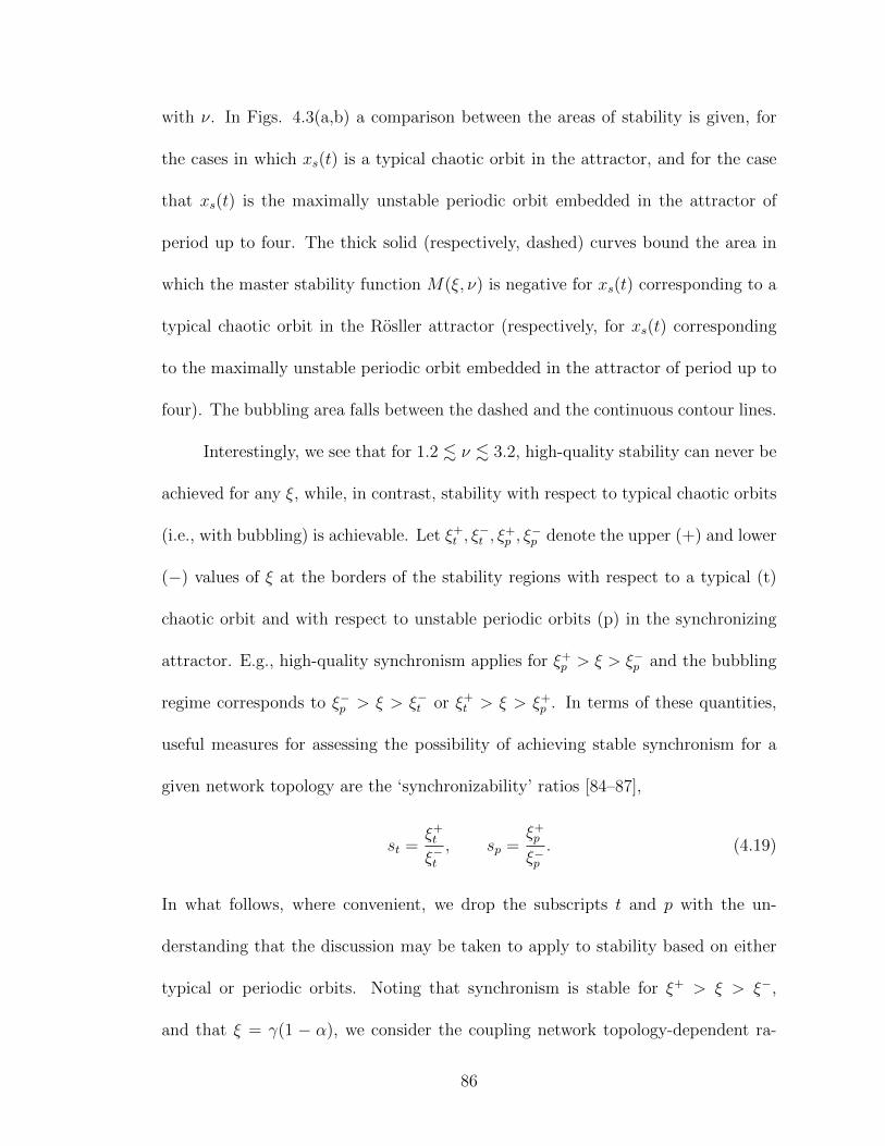
with ν. In Figs. 4.3(a,b) a comparison between the areas of stability is given, for

the cases in which xs(t) is a typical chaotic orbit in the attractor, and for the case

that xs(t) is the maximally unstable periodic orbit embedded in the attractor of

period up to four. The thick solid (respectively, dashed) curves bound the area in

which the master stability function M(ξ, ν) is negative for xs(t) corresponding to a

typical chaotic orbit in the Rosller attractor (respectively, for xs(t) corresponding

to the maximally unstable periodic orbit embedded in the attractor of period up to

four). The bubbling area falls between the dashed and the continuous contour lines.

Interestingly, we see that for 1.2 . ν . 3.2, high-quality stability can never be

achieved for any ξ, while, in contrast, stability with respect to typical chaotic orbits

(i.e., with bubbling) is achievable. Let ξ+t , ξ

−t , ξ

+p , ξ

−p denote the upper (+) and lower

(−) values of ξ at the borders of the stability regions with respect to a typical (t)

chaotic orbit and with respect to unstable periodic orbits (p) in the synchronizing

attractor. E.g., high-quality synchronism applies for ξ+p > ξ > ξ−p and the bubbling

regime corresponds to ξ−p > ξ > ξ−t or ξ+t > ξ > ξ+

p . In terms of these quantities,

useful measures for assessing the possibility of achieving stable synchronism for a

given network topology are the ‘synchronizability’ ratios [84–87],

st =ξ+t

ξ−t, sp =

ξ+p

ξ−p. (4.19)

In what follows, where convenient, we drop the subscripts t and p with the un-

derstanding that the discussion may be taken to apply to stability based on either

typical or periodic orbits. Noting that synchronism is stable for ξ+ > ξ > ξ−,

and that ξ = γ(1 − α), we consider the coupling network topology-dependent ra-

86

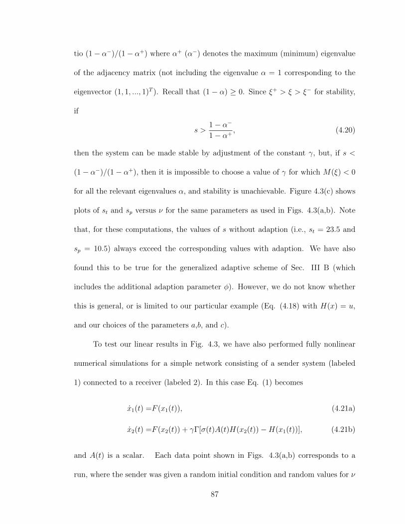
tio (1− α−)/(1− α+) where α+ (α−) denotes the maximum (minimum) eigenvalue

of the adjacency matrix (not including the eigenvalue α = 1 corresponding to the

eigenvector (1, 1, ..., 1)T ). Recall that (1 − α) ≥ 0. Since ξ+ > ξ > ξ− for stability,

if

s >1− α−

1− α+, (4.20)

then the system can be made stable by adjustment of the constant γ, but, if s <

(1− α−)/(1− α+), then it is impossible to choose a value of γ for which M(ξ) < 0

for all the relevant eigenvalues α, and stability is unachievable. Figure 4.3(c) shows

plots of st and sp versus ν for the same parameters as used in Figs. 4.3(a,b). Note

that, for these computations, the values of s without adaption (i.e., st = 23.5 and

sp = 10.5) always exceed the corresponding values with adaption. We have also

found this to be true for the generalized adaptive scheme of Sec. III B (which

includes the additional adaption parameter φ). However, we do not know whether

this is general, or is limited to our particular example (Eq. (4.18) with H(x) = u,

and our choices of the parameters a,b, and c).

To test our linear results in Fig. 4.3, we have also performed fully nonlinear

numerical simulations for a simple network consisting of a sender system (labeled

1) connected to a receiver (labeled 2). In this case Eq. (1) becomes

x1(t) =F (x1(t)), (4.21a)

x2(t) =F (x2(t)) + γΓ[σ(t)A(t)H(x2(t))−H(x1(t))], (4.21b)

and A(t) is a scalar. Each data point shown in Figs. 4.3(a,b) corresponds to a

run, where the sender was given a random initial condition and random values for ν

87

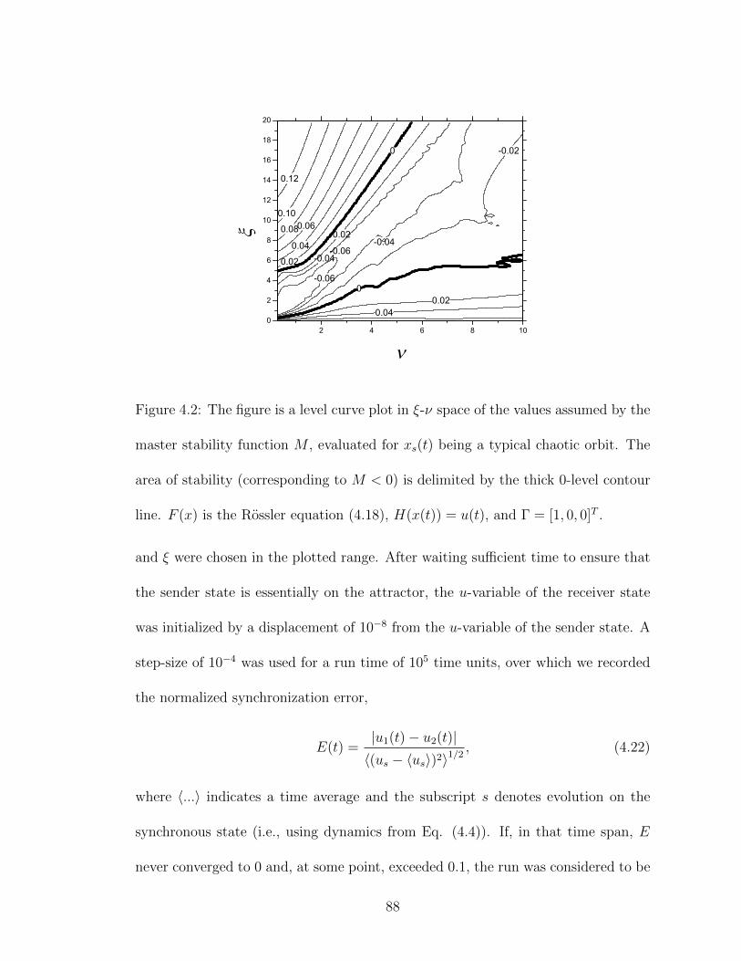
0.040.02

0

-0.02

-0.04

-0.04

-0.02

0

0.02

0.04

0.060.08

0.10

0.12

-0.06

-0.06

2 4 6 8 100

2

4

6

8

10

12

14

16

18

20

Figure 4.2: The figure is a level curve plot in ξ-ν space of the values assumed by the

master stability function M , evaluated for xs(t) being a typical chaotic orbit. The

area of stability (corresponding to M < 0) is delimited by the thick 0-level contour

line. F (x) is the Rossler equation (4.18), H(x(t)) = u(t), and Γ = [1, 0, 0]T .

and ξ were chosen in the plotted range. After waiting sufficient time to ensure that

the sender state is essentially on the attractor, the u-variable of the receiver state

was initialized by a displacement of 10−8 from the u-variable of the sender state. A

step-size of 10−4 was used for a run time of 105 time units, over which we recorded

the normalized synchronization error,

E(t) =|u1(t)− u2(t)|〈(us − 〈us〉)2〉1/2

, (4.22)

where 〈...〉 indicates a time average and the subscript s denotes evolution on the

synchronous state (i.e., using dynamics from Eq. (4.4)). If, in that time span, E

never converged to 0 and, at some point, exceeded 0.1, the run was considered to be

88

unstable (corresponding to an × in the figure). If E converged to 0, a 1% mismatch

in the Rossler parameter a was introduced to the receiver, and the run of duration 105

time units was repeated with an initial separation of 0. If, at any time during the run,

E ever exceeded 0.1, the run was considered to be bubbling (corresponding to a green

circle in the figure), otherwise the run was considered to be stable (corresponding

to a red triangle in the figure). We see that the master stability computations of

the high-quality stable, bubbling, and unstable regions (the solid and dashed lines)

correspond well with these results. We also did a sampling of points up to period

5 and did not find that this altered our results. From Fig. 4.3(a), we observe the

presence of a few green circles (i.e, bubbling) within the high-quality synchronization

area, delimited by the dashed line. In reference to this observation, we note that (i)

for the case in which a small parameter mismatch is present, the synchronization

error is expected to vary smoothly with parameter variation, and there is no sharp

transition from the stable to the bubbling regime; and (ii) our computations show

that close to the dashed line, the master stability function associated with the most

unstable invariant set embedded in the attractor is rather small. Facts (i) and (ii)

explain our difficulty in using our nonlinear computations to clearly separate the

bubbling from the stable regions about the dashed line in Fig. 4.3(a). An important

point concerning Figs. 4.3(a,b) is that the area associated with bubbling in Fig.

4.3(a) is rather substantial. This observation would become particularly important

in experimental realizations of adaptive synchronization, since small mismatches in

the parameters and noise cannot be avoided in experiments.

Figure 4.4 shows a sample plot of the normalized synchronization error E(t),

89

versus t. We implemented our adaptive strategy with values of ν = 2.5 and γ = 5,

corresponding to the bubbling regime (see Fig. 4.3), A(t) = 1, and the receiver

has 0.1% mismatch in the parameter a. The two insets are zooms showing phase-

space projections in the plane (u2, v2), over two different time intervals. Inset (b)

corresponds to a range of time between bursts (E(t) < 5 × 10−2) and shows that

during this time the orbit is essentially that of a typical chaotic orbit. Inset (a)

shows the orbit trajectory for a range of time during which a burst is growing. It is

seen from inset (b) that during the time range of the growing burst the orbit closely

follows a period 4 orbit embedded in the attractor. The burst is evidently caused

by the instability of this period 4 orbit to perturbations that are transverse to the

synchronization manifold.

We have also performed numerical master stability computations for our gen-

eralized adaptive strategy, presented in Sec. IIIb. This is shown in Fig. 4.5, where

the ξ+(φ) and ξ−(φ) curves, corresponding respectively to the largest (smallest) val-

ues of ξ for which M(ξ, φ) > 0 (M(ξ, φ) < 0), are plotted versus φ for three different

values of ν = [0.1, 2.0, 6.0] for typical chaotic orbits. For small ν (e.g., ν = 0.1

in the figure), the range of stability [ξ−, ξ+] is almost independent of φ, while for

larger values of ν the choice of φ can significantly affect the ξ-range of stability. As

expected, at φ = 2, ξ+(φ) and ξ−(φ) are independent of ν.

Finally, we investigated whether, for our coupled systems with adaptation,

bubbling can be caused by a slow drift in the coupling strength. For this purpose

90

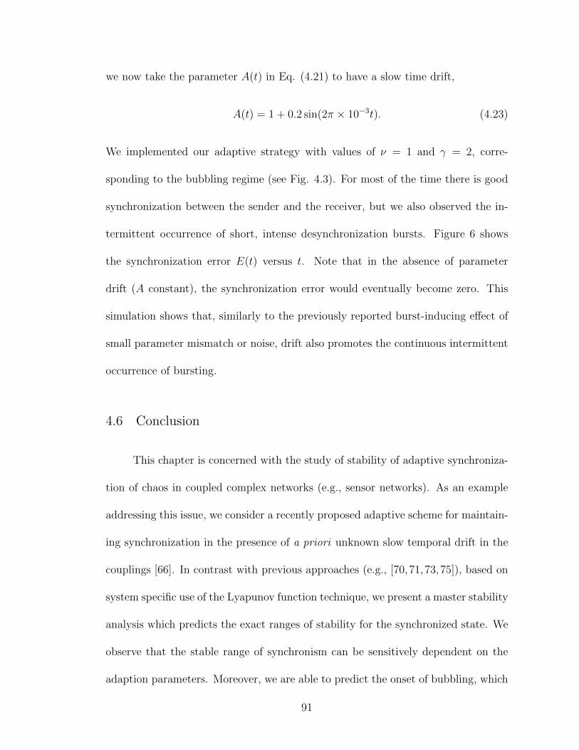
we now take the parameter A(t) in Eq. (4.21) to have a slow time drift,

A(t) = 1 + 0.2 sin(2π × 10−3t). (4.23)

We implemented our adaptive strategy with values of ν = 1 and γ = 2, corre-

sponding to the bubbling regime (see Fig. 4.3). For most of the time there is good

synchronization between the sender and the receiver, but we also observed the in-

termittent occurrence of short, intense desynchronization bursts. Figure 6 shows

the synchronization error E(t) versus t. Note that in the absence of parameter

drift (A constant), the synchronization error would eventually become zero. This

simulation shows that, similarly to the previously reported burst-inducing effect of

small parameter mismatch or noise, drift also promotes the continuous intermittent

occurrence of bursting.

4.6 Conclusion

This chapter is concerned with the study of stability of adaptive synchroniza-

tion of chaos in coupled complex networks (e.g., sensor networks). As an example

addressing this issue, we consider a recently proposed adaptive scheme for maintain-

ing synchronization in the presence of a priori unknown slow temporal drift in the

couplings [66]. In contrast with previous approaches (e.g., [70,71,73,75]), based on

system specific use of the Lyapunov function technique, we present a master stability

analysis which predicts the exact ranges of stability for the synchronized state. We

observe that the stable range of synchronism can be sensitively dependent on the

adaption parameters. Moreover, we are able to predict the onset of bubbling, which

91

occurs when the synchronized state is stable for typical chaotic orbits but is unstable

for certain unstable periodic orbits within the synchronized chaotic attractor. We

define stability to be high quality when the synchronized state is stable with respect

to all the orbits embedded in the attractor and numerically find the regions of ‘high

quality stability’ for a given system of interest. We also found that, for our coupled

systems with adaptation, bubbling can be caused by a slow drift in the coupling

strength, in addition to small noise and small mismatch in F . We emphasize that,

since parameter mismatch, noise and drift are ubiquitous in experimental situations,

and since (e.g., Fig. 4.3(a)) bubbling can occupy substantial regions of parameter

space, consideration of bubbling can be expected to be essential for determining the

practical feasibility of chaos synchronization applications.

92

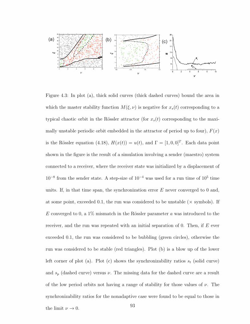
Figure 4.3: In plot (a), thick solid curves (thick dashed curves) bound the area in

which the master stability function M(ξ, ν) is negative for xs(t) corresponding to a

typical chaotic orbit in the Rossler attractor (for xs(t) corresponding to the maxi-

mally unstable periodic orbit embedded in the attractor of period up to four), F (x)

is the Rossler equation (4.18), H(x(t)) = u(t), and Γ = [1, 0, 0]T . Each data point

shown in the figure is the result of a simulation involving a sender (maestro) system

connected to a receiver, where the receiver state was initialized by a displacement of

10−8 from the sender state. A step-size of 10−4 was used for a run time of 105 time

units. If, in that time span, the synchronization error E never converged to 0 and,

at some point, exceeded 0.1, the run was considered to be unstable (× symbols). If

E converged to 0, a 1% mismatch in the Rossler parameter a was introduced to the

receiver, and the run was repeated with an initial separation of 0. Then, if E ever

exceeded 0.1, the run was considered to be bubbling (green circles), otherwise the

run was considered to be stable (red triangles). Plot (b) is a blow up of the lower

left corner of plot (a). Plot (c) shows the synchronizability ratios st (solid curve)

and sp (dashed curve) versus ν. The missing data for the dashed curve are a result

of the low period orbits not having a range of stability for those values of ν. The

synchronizability ratios for the nonadaptive case were found to be equal to those in

the limit ν → 0.93

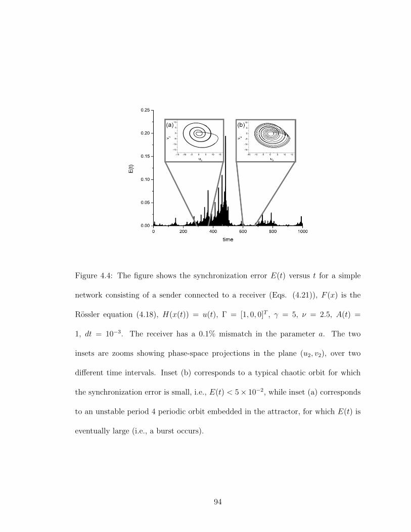
Figure 4.4: The figure shows the synchronization error E(t) versus t for a simple

network consisting of a sender connected to a receiver (Eqs. (4.21)), F (x) is the

Rossler equation (4.18), H(x(t)) = u(t), Γ = [1, 0, 0]T , γ = 5, ν = 2.5, A(t) =

1, dt = 10−3. The receiver has a 0.1% mismatch in the parameter a. The two

insets are zooms showing phase-space projections in the plane (u2, v2), over two

different time intervals. Inset (b) corresponds to a typical chaotic orbit for which

the synchronization error is small, i.e., E(t) < 5× 10−2, while inset (a) corresponds

to an unstable period 4 periodic orbit embedded in the attractor, for which E(t) is

eventually large (i.e., a burst occurs).

94

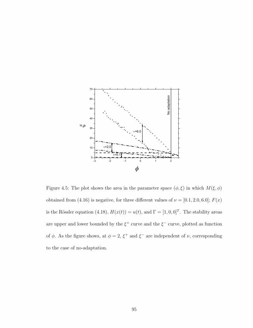
-3 -2 -1 0 1 20

10

20

30

40

50

60

70

=0.1

=2.0

=6.0

No

adap

tatio

n

Figure 4.5: The plot shows the area in the parameter space (φ, ξ) in which M(ξ, φ)

obtained from (4.16) is negative, for three different values of ν = [0.1, 2.0, 6.0]; F (x)

is the Rossler equation (4.18), H(x(t)) = u(t), and Γ = [1, 0, 0]T . The stability areas

are upper and lower bounded by the ξ+ curve and the ξ− curve, plotted as function

of φ. As the figure shows, at φ = 2, ξ+ and ξ− are independent of ν, corresponding

to the case of no-adaptation.

95

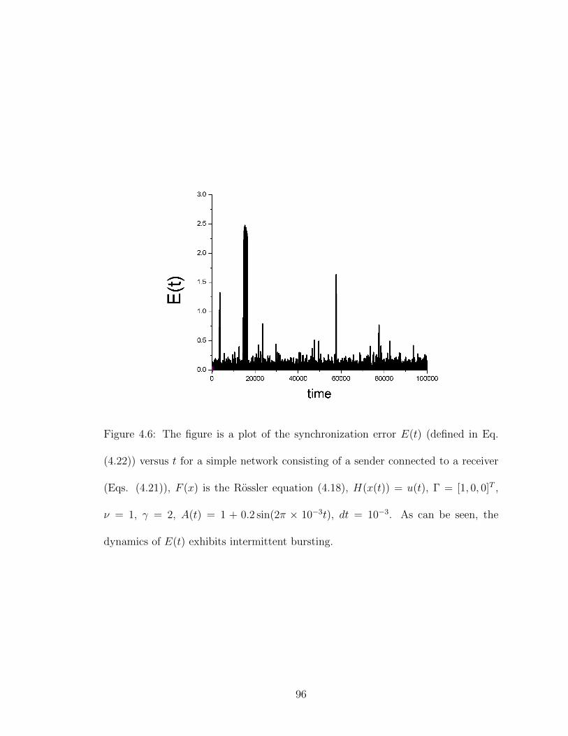
Figure 4.6: The figure is a plot of the synchronization error E(t) (defined in Eq.

(4.22)) versus t for a simple network consisting of a sender connected to a receiver

(Eqs. (4.21)), F (x) is the Rossler equation (4.18), H(x(t)) = u(t), Γ = [1, 0, 0]T ,

ν = 1, γ = 2, A(t) = 1 + 0.2 sin(2π × 10−3t), dt = 10−3. As can be seen, the

dynamics of E(t) exhibits intermittent bursting.

96

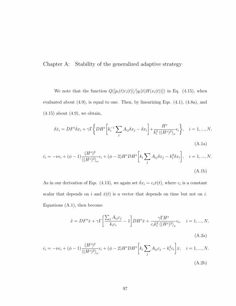
Chapter A: Stability of the generalized adaptive strategy

We note that the function Q([pi(t)ri(t)]/[qi(t)H(xi(t))]) in Eq. (4.15), when

evaluated about (4.9), is equal to one. Then, by linearizing Eqs. (4.1), (4.8a), and

(4.15) about (4.9), we obtain,

δxi = DF sδxi + γΓ

DHs

[k−1i

∑j

Aijδxj − δxi]+

Hs

k2i 〈(Hs)2〉ν

εi

, i = 1, ..., N,

(A.1a)

εi = −νεi + (φ− 1)(Hs)2

〈(Hs)2〉νεi + (φ− 2)HsDHs

[ki∑j

Aijδxj − k2i δxi

], i = 1, ..., N.

(A.1b)

As in our derivation of Eqs. (4.13), we again set δxi = cix(t), where ci is a constant

scalar that depends on i and x(t) is a vector that depends on time but not on i.

Equations (A.1), then become

˙x = DF sx+ γΓ

[∑j Aijcj

kici− 1

]DHsx+

γΓHs

cik2i 〈(Hs)2〉ν

εi, i = 1, ..., N,

(A.2a)

εi = −νεi + (φ− 1)(Hs)2

〈(Hs)2〉νεi + (φ− 2)HsDHs

[ki∑j

Aijcj − k2i ci

]x, i = 1, ..., N.

(A.2b)

97

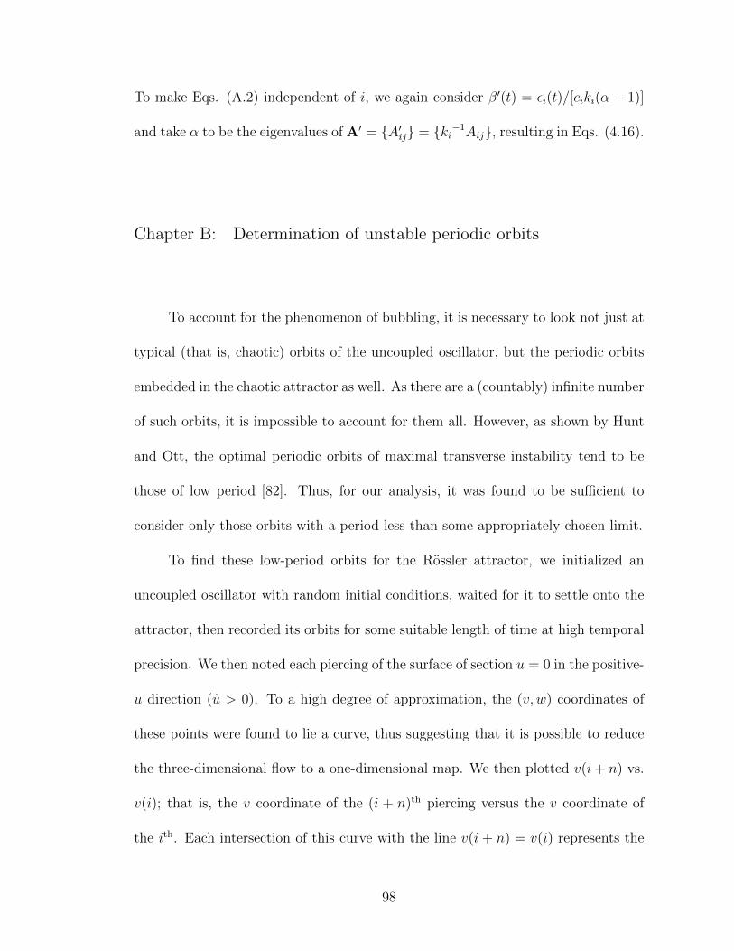
To make Eqs. (A.2) independent of i, we again consider β′(t) = εi(t)/[ciki(α − 1)]

and take α to be the eigenvalues of A′ = A′ij = ki−1Aij, resulting in Eqs. (4.16).

Chapter B: Determination of unstable periodic orbits

To account for the phenomenon of bubbling, it is necessary to look not just at

typical (that is, chaotic) orbits of the uncoupled oscillator, but the periodic orbits

embedded in the chaotic attractor as well. As there are a (countably) infinite number

of such orbits, it is impossible to account for them all. However, as shown by Hunt

and Ott, the optimal periodic orbits of maximal transverse instability tend to be

those of low period [82]. Thus, for our analysis, it was found to be sufficient to

consider only those orbits with a period less than some appropriately chosen limit.

To find these low-period orbits for the Rossler attractor, we initialized an

uncoupled oscillator with random initial conditions, waited for it to settle onto the

attractor, then recorded its orbits for some suitable length of time at high temporal

precision. We then noted each piercing of the surface of section u = 0 in the positive-

u direction (u > 0). To a high degree of approximation, the (v, w) coordinates of

these points were found to lie a curve, thus suggesting that it is possible to reduce

the three-dimensional flow to a one-dimensional map. We then plotted v(i+ n) vs.

v(i); that is, the v coordinate of the (i + n)th piercing versus the v coordinate of

the ith. Each intersection of this curve with the line v(i + n) = v(i) represents the

98

v coordinate of an initial condition for an orbit that starts on the surface of section

and returns to its original position after n piercing of the surface of section. With

two coordinates (namely u and v) known, all that remains is to find the value of w

such that (0, v, w) lies on the attractor.

Of course, for n > 1, many of these intersections will be redundant, as every

period n orbit pierces the surface of section n times, thus producing n intersections

on the curve. In addition, each curve will have intersections corresponding to orbits

of any period that is a factor of n. As an example, consider the curve v(i + 4) vs.

v(i). The Rossler system used in this paper has three Period 4 orbits, one Period

2 orbit and one Period 1 orbit. Thus, the number of times v(i + 4) vs. v(i) will

intersect v(i+ 4) = v(i) is 3× 4 + 1× 2 + 1× 1 = 15.

As these orbits are inherently unstable, error accumulated through numerical

integration can result in a trajectory leaving the periodic orbit after only a small

number of periods. Thus, for the long term computation of Lyapunov exponents to

obtain the master stability function, it is advisable to compute the trajectory for

only a single period, then return the oscillator to its initial position (u, v, w), and

repeat as often as needed.

99

Bibliography

[1] S. Boccaletti, V. Latora, Y. Moreno, M. Charles, D.-U. Wang, “Complex net-works: Structure and dynamics,” Phys. Rpts. 424,175 (2006).

[2] A.E. Motter, M.A. Matias, J. Kurths and E. Ott, “Dynamics on ComplexNetworks and Applications,” Physica D 224, vii (2006).

[3] Y. Kuramoto in International Symposium on Mathematrical Problems in Theo-retical Physics, Lecture Notes in Physics, edited by H. Araki (Springer-Verlag,Berlin 1975), vol. 39.

[4] Y. Kuramoto, Chemical Oscillators, Waves and Turbulence (Springer, NewYork, 1984).

[5] S.H. Strogatz, “From Kuramoto to Crawford: exploring the onset of synchro-nization in populations of coupled oscillators,” Physica D 143, 1 (2000).

[6] E. Ott, Chaos in Dynamical Systems (Cambridge University Press, second edi-tion, 2002).

[7] J.A. Acebron, L.L. Bonilla, C.J.P. Cincente, R. Ritort and R. Spigler, “TheKuramoto model: A simple paradigm for synchronization phenomena,” Rev.Mod. Phys. 77, 137 (2005).

[8] E. Ott and T.M. Antonsen, “Low dimensional behavior of large systems ofglobally coupled oscillators,” Chaos 18, 037113 (2008).

[9] E. Ott and T.M. Antonsen, “Long time evolution of phase oscillator systems,”Chaos 19, 023117 (2009).

100

[10] J. Stout, M. Whiteway, E. Ott, M. Girvan and T.M. Antonsen, “Local syn-chronization in complex networks of coupled oscillators,” Chaos 21, 025109(2011).

[11] J. Gomez-Gandenes, Y. Moreno and A. Arenas, “From scale-free to Erdos-Rnyinetworks,” Phys. Rev. E 73, 056124 (2006).

[12] M. Brede, “Locals vs. global synchronization in networks of non-identical Ku-ramoto oscillators,” Eur. Phys. J. B 62, 87 (2008).

[13] J.G. Restrepo, E. Ott and B.R. Hunt, “Onset of synchronization in large net-works of coupled oscillators,” Phys. Rev. E 71, 036151 (2005); Physica D 224,114 (2006).

[14] T. Ichimoiya, “Frequency synchronization in a random oscillator network,”Phys. Rev. E 70, 026116 (2004).

[15] L. M. Alonso, J.A. Allende and G.B. Mindlen, “Dynamical origin of complexmotor patterns,” Eur. Phys. J. D 60, 361 (2010).

[16] A. Ghosh, D. Roy and V.K. Jirsa, “Simple model for bursting dynamics ofneurons,” Phys. Rev. E 80, 041930 (2009).

[17] M.M. Abduelreheme and E. Ott, “Low dimensional description of pedestrian-induced oscillation of the Millennium Bridge,” Chaos 19, 013129 (2009).

[18] L.M. Childs and S.H. Strogatz, “Stability diagram for the forced Kuramotomodel,” Chaos 18, 043128 (2008).

[19] S.A. Marvel and S.H. Strogatz, “Invariant submanifold for series arrays ofJosephson junctions,” Chaos 19, 013132 (2009).

[20] L.F. Lafuerza, P. Colet and R. Toral, “Nonuniversal Results Induced by Diver-sity Distribution in Coupled Excitable Systems,” Phys. Rev. Lett. 105, 084101(2010).

[21] K.H. Nagai and H. Kori, “Noise-induced synchronization of a large populationof globally coupled nonidentical oscillators,” Phys. Rev. E 81, 065202 (2010).

[22] E.A. Martens, E. Barreto, S.H. Strogatz, E. Ott, P. So and T.M. Antonsen,“Exact results for the Kuramoto model with a bimodal frequency distribution,”Phys. Rev. E 79, 026204 (2009).

101

[23] D. Pazo and E. Montbrio, “Existence of hysteresis in the Kuramoto model withbimodal frequency distributions,” Phys. Rev. E 80, 046215 (2009).

[24] W.S. Lee, E. Ott and T.M. Antonsen, “Large Coupled Oscillator Systems withHeterogeneous Interaction Delays,” Phys. Rev. Lett. 103, 044101 (2009).

[25] Z. Levajic and A. Pikovsky, “Phase resetting of collective rhythm in ensemblesof oscillators,” Phys. Rev. E 82, 056202 (2010).

[26] P. So, B.C. Cotton and E. Barretto, “Synchronization in interacting populationsof heterogeneous oscillators with time-varying coupling,” Chaos 18, 037114(2008).

[27] Y. Kawamura, H. Nakao, K. Arai, H. Kori and Y. Kuramoto, “Phase syn-chronization between collective rhythms of globally coupled oscillator groups:Noiseless nonidentical case,” Chaos 20, 043110 (2010).

[28] A. Pikovsky and M. Rosenblum, “Partially Integrable Dynamics of HierarchicalPopulations of Coupled Oscillators,” Phys. Rev. Lett. 101, 264103 (2008).

[29] C.R. Lang, “Chimera states in heterogeneous networks,” Chaos 19, 013113(2009).

[30] C.R. Laing, “The dynamics of chimera states in heterogeneous Kuramoto net-works,” Physica D 238, 1569 (2009).

[31] E.A. Martens, “Bistable chimera attractors on a triangular network of oscillatorpopulations,” Phys. Rev. E 82, 016216 (2010).

[32] G. Borydugov, A. Pikovsky and M. Rosenblum, “Self-emerging and turbulentchimeras in oscillator chains,” Phys. Rev. E 82, 035205 (2010).

[33] E.A. Martens, “Chimeras in a network of three oscillator populations withvarying network topology,” Chaos 20, 043122 (2010).

[34] M.E.J. Newman, “The Structure and Function of Complex Networks” SIAMReview 45, 167 (2003) Sec. 4.2.1.

[35] J.G. Restrepo, E. Ott and B.R. Hunt, “Approximating the largest eigenvalueof network adjacency matrices,” Phys. Rev. E 76, 056119 (2007).

[36] S. Chauhan, M. Girvan, E. Ott, “Spectral properties of networks with commu-nity structure,” Phys. Rev. E 80, 056114 (2009).

102

[37] L. Pecora and T. L. Carroll, “Master Stability Functions for Synchronized Cou-pled Systems,” Phys. Rev. Lett. 80, 2109 (1998).

[38] H. Fujisaka and T. Yamada, “Stability Theory of Synchronized Motion inCoupled-Oscillator Systems,” Prog. Theor. Phys. 69, 32 (1983).

[39] In Fig. 2.10 we have omitted a curve on which there is a transcritical bifurcationfrom one fixed point to another (i.e., an interchange of stability and instabilityas the two fixed points pass through each other). In this case there is a singleSS attractor on both sides of the bifurcation. The omitted bifurcation curve isa 90 arc of the radious one circle centered at (ω0, ∆) = (0, 1) and extends frompoint c to the origin.

[40] A simulation length of 2, 000 time units (with time averaging done over the last1, 000 units) is far more than is usually required. It was usually sufficient to runthe simulations for 500 time units with time averaging done over the last 100units. The overly long simulations were done to ensure maximum accuracy.

[41] M.I. Freidlin, A.D. Wentzell and J. Szucs, Random Perturbations of DynamicalSystems (Springer-Verlag, New York, 1998).

[42] T. M. Antonsen, Jr., R. T. Faghih, M. Girvan, E. Ott and J. Platig, “Externalperiodic driving of large systems of globally coupled phase oscillators” Chaos18 037112 (2008).

[43] G. Barlev, M. Girvan and E. Ott, “Map model for synchronization of systemsof many coupled oscillators,” Chaos 20, 023109 (2010).

[44] O. Popovych, Y. Maistrenko, P. Tass, “Phase chaos in coupled oscillators,”Phys. Rev. E 71, 065201 (2005).

[45] M. Wolfrum, O. Omel’chenko, “Chimera states are chaotic transients,” Phys.Rev. E 84, 015201 (2011).

[46] I. Shimada and T. Nagashima, “A numerical approach to ergodic problem ofdissipative dynamical systems,” Prog. Theoret. Phys. 61, 1605 (1979).

[47] K. Ramasubramanian and M.S. Sriram, “A comparative study of computationof Lyapunov spectra with different algorithms,” Physica D 139 72 (2000).

[48] QR decomposition was performed using the LAPACK routine xGEQR2P, whichuses Householder reflections while guaranteeing positive entries for the diagonalterms of the matrix R. See J. Demmel, M. Hoemmen, Y. Hida and E.J. Riedy,

103

“Nonnegative Diagonals and High Performance on Low-Profile Matrices fromHouseholder QR,” SIAM Journal on Scientific Computing, 31 2832 (2009).

[49] We have reproduced the results of Ref. [44] using our Lyapunov exponent com-putation code. Thus, the difference between our results and those of Ref. [44]are not due to coding differences, but rather reflect the different situationstreated.

[50] The single oscillator hypothesis presents a small problem: it overdescribes thesystem by one vector, since there are N oscillators which should each have acorresponding Lyapunov vector ~vSOHj , but there is also the rotation vector ~v0,specified by Eq. (3.12). From a practical perspective, the issue is moot dueto the degeneracy of the Lyapunov spectrum: for small values of k, there aremultiple predicted Lyapunov exponents extremely near zero, any one of whichcould be “missing,” and at large k, the Lyapunov vectors converge to h∞ (Eq.(3.21)) so closely that they are nearly degenerate.

[51] V. S. Afraimovich, N. N. Verichev, and M. I. Rabinovich, “Stochastic synchro-nization of oscillations in dissipative systems,” Inv. VUZ Radiofiz. RPQAEC29, 795 (1986).

[52] K. M. Cuomo and A. V. Oppenheim, “Circuit implementation of synchronizedchaos with applications to communications,” Phys. Rev. Lett. 71, 65 (1993).

[53] A. Argyris, M. Hamacher, K. E. Chlouverakis, A. Bogris, and D. Syvridis, “Pho-tonic Integrated Device for Chaos Applications in Communications,” Phys. Rev.Lett. 100, 194101 (2008).

[54] M. Feki, “An adaptive chaos synchronization scheme applied to secure commu-nication,” Chaos, Solitons and Fractals 18, 141 (2003).

[55] H. D. I. Abarbanel, D. R. Creveling, and J. M. Jeanne, “Estimation of param-eters in nonlinear systems using balanced synchronization,” Phys. Rev. E 77,016208 (2008).

[56] D. R. Creveling, P. E. Gill, and H. D. I. Abarbanel, “State and parameterestimation in nonlinear systems as an optimal tracking problem,” Phys. Lett.A 372, 2640 (2008).

[57] J. C. Quinn, P. H. Bryant, D. R. Creveling, S. R. Klein, and H. D. I. Abar-banel, “Parameter and state estimation of experimental chaotic systems usingsynchronization,” Phys. Rev. E 80, 016201 (2009).

104

[58] F. Sorrentino and E. Ott, “Using synchronization of chaos to identify the dy-namics of unknown systems,” Chaos 19, 033108 (2009a).

[59] P. So, E. Ott, and W. P. Dayawansa, “Observing chaos: Deducing and trackingthe state of a chaotic system from limited observation,” Phys. Rev. E 49, 2650(1994).

[60] G. S. Duane, J. J. Tribbia, and J. B. Weiss, “Synchronicity in predictive mod-elling: a new view of data assimilation,” Nonlinear processes in Geophysics 13,601 (2006).

[61] F. Sorrentino and E. Ott, “Using synchronism of chaos for adaptive learning oftime-evolving network topology,” Phys. Rev. E 79, 016201 (2009b).

[62] S. Hayes, C. Grebogi, and E. Ott, “Communicating with chaos,” Phys. Rev.Lett. 70, 3031 (1993).

[63] V. Dronov, M. Hendrey, T. M. Antonsen, and E. Ott, “Communication with achaotic traveling wave tube microwave generator,” Chaos 14, 30 (2004).

[64] L. S. Tsimring and M. M. Sushchik, “Multiplexing chaotic signals using syn-crhonization,” Phys. Lett. A 213, 155 (1996).

[65] N. Sharma and E. Ott, “Exploiting synchronization to combat channel dis-tortions in communication with chaotic systems,” Int. J. Bif. Chaos 10, 777(2000).

[66] F. Sorrentino and E. Ott, “Adaptive Synchronization of Dynamics on EvolvingComplex Networks,” Phys. Rev. Lett. 100, 114101 (2008).

[67] B. Ravoori, A. B. Cohen, A. V. Setty, F. Sorrentino, T. E. Murphy,E. Ott, and R. Roy, “Adaptive synchronization of coupled chaotic oscillators,”arXiv:0907.3894 (2009).

[68] F. Mossayebi, H. K. Qammar, and T. T. Hartley, “Adaptive estimation andsynchronization of chaotic systems,” Phys. Lett. A 161, 255 (1991).

[69] C. R. Johnson Jr. and J. S. Thorp, “An adaptive calibration algorithm forsynchronized chaos,” IEEE Sig. Proc. Lett. 1, 194 (1994).

[70] U. Parlitz and L. Kocarev, “Multichannel communication using autosynchro-nization,” Int. J. Bif. Chaos 6, 581 (1996).

105

[71] C. W. Wu, T. Yang, and L. O. Chua, “On adaptive synchronization and controlof nonlinear dynamical systems,” Int. J. Bif. Chaos 6, 455 (1996).

[72] L. O. Chua, T. Yang, G.-Q. Zhong, and C. W. Wu, “Adaptive synchronizationof Chua’s oscillators,” Int. J. Bif. Chaos 6, 189 (1996).

[73] M. di Bernardo, “An adaptive approach to the control and synchronization ofcontinuous-time chaotic systems,” Int. J. Bif. Chaos 6, 557 (1996).

[74] D. J. Sobiski and J. S. Thorp, “PDMA-1: chaotic communication via the ex-tended Kalman filter,” IEEE Trans. Circ. Syst. I 45, 194 (1998).

[75] T.-L. Liao, “Adaptive syncrhonization of two Lorenz systems,” Chaos SolitonsFractals 9, 1555 (1998).

[76] C. Zhou and J. Kurths, “Dynamical weights and enhanced syncrhonization inadaptive complex networks,” Phys. Rev. Lett. 96, 164102 (2006).

[77] P. De Lellis, M. di Bernardo, and F. Garofalo, “Synchronization of complexnetworks through local adaptive coupling,” Chaos 18, 037110 (2008).

[78] P. Ashwin, J. Buescu, and I. N. Stewart, “Bubbling of attractors and synchro-nisation of chaotic oscillators,” Phys. Lett. A 193, 126 (1994a).

[79] P. Ashwin, J. Buescu, and I. N. Stewart, “From attractor to chaotic saddle: atale of transverse instability,” Nonlinearity 9, 703 (1994b).

[80] S. C. Venkataramani, B. R. Hunt, and E. Ott, “Bubbling transition,” Phys.Rev. E 54, 1346 (1996).

[81] In addition, to desynchronism bursts, it is also possible that a large desyn-chronization orbit event can result in capture of the system orbit on a desyn-chronized attractor with a so-called riddled basin of attraction (e.g., see Refs.[6,78–80,89]). This possibility, although a typical occurrence in such situations,did not manifest itself in the particular system used for our numerical studies inSec. IV. Thus we, henceforth, restrict our discussion to the case that bubblingis associated with bursts.

[82] B. R. Hunt and E. Ott, “Optimal periodic orbits of chaotic systems,” Phys.Rev. Lett. 76, 2254 (1996).

[83] J. G. Restrepo, E. Ott, and B. R. Hunt, “Spatial patterns of desynchronizationbursts in networks,” Phys. Rev. E 69, 066215 (2004).

106

[84] M. Barahona and L. Pecora, “Synchronization in small-world systems,” Phys.Rev. Lett. 89, 054101 (2002).

[85] T. Nishikawa, A. Motter, Y. Lai, and F. Hoppensteadt, “Heterogeneity in os-cillator networks: are smaller worlds easier to synchronize?,” Phys. Rev. Lett.91, 014101 (2003).

[86] M. Chavez, D. Huang, A. Amann, H. Hentschel, and S. Boccaletti, “Syn-chronization is enhanced in weighted complex networks,” Phys. Rev. Lett. 94,218701 (2005).

[87] D. Hwang, M. Chavez, A. Amann, and S. Boccaletti, “Synchronization in com-plex networks with age ordering,” Phys. Rev. Lett. 94, 138701 (2005).

[88] F. Sorrentino, M. di Bernardo, F. Garofalo, and G. Chen, “Controllability ofcomplex networks via pinning,” Phys. Rev. E 75, 046103 (2007).

[89] E. Ott and J. C. Sommerer, “Blowout bifurcations: the occurrence of riddledbasins and on-off intermittency,” Phys. Lett. A 188, 39 (1994).

107