NBER WORKING PAPER SERIES

USE OF PROPENSITY SCORES IN NON-LINEAR RESPONSE MODELS:THE CASE FOR HEALTH CARE EXPENDITURES

Anirban BasuDaniel Polsky

Willard G. Manning

Working Paper 14086http://www.nber.org/papers/w14086

NATIONAL BUREAU OF ECONOMIC RESEARCH1050 Massachusetts Avenue

Cambridge, MA 02138June 2008

We are grateful to Paul J. Rathouz and Tyler J. VanderWeele for their suggestions on an earlier draftof this paper. We also thank seminar participants at the University of Chicago, York and Glasgowfor their comments on this work. The views expressed in this paper are those of the authors and notnecessarily those of the National Bureau of Economic Research, the University of Chicago, or theUniversity of Pennsylvania. All errors are our own.

NBER working papers are circulated for discussion and comment purposes. They have not been peer-reviewed or been subject to the review by the NBER Board of Directors that accompanies officialNBER publications.

© 2008 by Anirban Basu, Daniel Polsky, and Willard G. Manning. All rights reserved. Short sectionsof text, not to exceed two paragraphs, may be quoted without explicit permission provided that fullcredit, including © notice, is given to the source.

Use of Propensity Scores in Non-Linear Response Models: The Case for Health Care ExpendituresAnirban Basu, Daniel Polsky, and Willard G. ManningNBER Working Paper No. 14086June 2008JEL No. C01,C21,I10

ABSTRACT

Under the assumption of no unmeasured confounders, a large literature exists on methods that canbe used to estimating average treatment effects (ATE) from observational data and that spans regressionmodels, propensity score adjustments using stratification, weighting or regression and even the combinationof both as in doubly-robust estimators. However, comparison of these alternative methods is sparsein the context of data generated via non-linear models where treatment effects are heterogeneous, suchas is in the case of healthcare cost data. In this paper, we compare the performance of alternative regressionand propensity score-based estimators in estimating average treatment effects on outcomes that aregenerated via non-linear models. Using simulations, we find that in moderate size samples (n= 5000),balancing on estimated propensity scores balances the covariate means across treatment arms but failsto balance higher-order moments and covariances amongst covariates, raising concern about its usein non-linear outcomes generating mechanisms. We also find that besides inverse-probability weighting(IPW) with propensity scores, no one estimator is consistent under all data generating mechanisms.The IPW estimator is itself prone to inconsistency due to misspecification of the model for estimatingpropensity scores. Even when it is consistent, the IPW estimator is usually extremely inefficient. Thuscare should be taken before naively applying any one estimator to estimate ATE in these data. Wedevelop a recommendation for an algorithm which may help applied researchers to arrive at the optimalestimator. We illustrate the application of this algorithm and also the performance of alternative methodsin a cost dataset on breast cancer treatment.

Anirban BasuSection of General Internal MedicineDepartment of MedicineUniversity of Chicago5841 S. Maryland AvenueMC-2007, AMD B226CChicago, IL 60637and NBERabasu@medicine.bsd.uchicago.edu

Daniel PolskyUniversity of Pennsylvania School of MedicineDivision of General Internal Medicine423 Guardian Drive, Blockley Hall, Rm 1212Philadelphia, PA 19104polsky@mail.med.upenn.edu

Willard G. ManningUniversity of ChicagoHarris School of Public Policy Studies1155 East 60th Street, Room 176Chicago, IL 60637w-manning@uchicago.edu

2

1. Introduction

Average treatment effect (ATE) and other mean treatment effect parameters (such as

the Effect on the Treated) are quintessential components of economic evaluation

(Heckman and Robb, 1985; Heckman 1990, 1992; Manski and Garfinkel, 1992; Heckman

and Smith, 1998; Dehejia, 2005). Researchers often rely on observational data to

estimate these effects because they are relatively inexpensive to obtain and often provide

population coverage. However assignment to treatment is typically not random in these

data, but is instead based on several confounding factors that may also affect outcomes.

The traditional way to adjust for these confounding variables is to do some variant of

regression analysis, where the effect of the treatment is estimated after holding the levels

of a variety of confounding covariates constant across the treatment groups (Altman,

1998; Greenland et al, 1999). More recently, propensity score methods have been

proposed and used as alternatives for estimating these effects. In such methods, one

estimates how various characteristics affect the probability of treatment receipt, creates a

score based on this estimation and then compares observed outcomes between treated

and untreated subjects conditional on this score (Rosenbaum and Rubin, 1983). The

theory of propensity scores suggests that, conditional on this scalar propensity score, all

of the selection bias generated by differences in observed covariate values between the

treatment and control group can be removed.

Proponents of propensity score methods have highlighted the robustness of these

methods in comparison to regression methods when there are multiple covariates to

adjust for, even though the later can be much more efficient when appropriately specified

(Rosenbaum, 1987; Rubin and Thomas, 1996; Rosenbaum, 2002; Angrist and Hahn,

3

2004) while misspecified models for estimating the propensity scores can lead to biases in

estimating treatment effects (Drake, 1993). However, these results on comparing

propensity score methods to regression methods have been primarily established only in

the context of linear data generating mechanisms.

In this work, we will extend this comparison to outcomes data that are generated

under a non-linear continuous data generating mechanism implying that treatment effects

are heterogeneous across the population.a We will use health care costs or expenditures

as the prototype example of such an outcome measure, which also have non-normal

characteristics: non-negative values and skewness on the right hand side. Many other

outcomes in economics carry similar features – earnings (Dehejia and Wahba, 1999),

income (Jalan and Ravallion, in press) and a variety of marketing outcomes such as sales

(Rubin and Waterman, 2006), - and our results extend readily to these outcomes as well.

There is a large literature since the 1960s that addresses skewness in outcome (e.g.,

cost or other) data and appropriate non-linear covariate adjustment methods that go with it

(Box and Cox, 1964; McCullagh and Nelder, 1983; Mullahy 1998; Blough et al., 1999;

Manning and Mullahy, 2001). For health care costs and expenditures, it is typical to find a

fraction of patients with expenditures much larger than the median patient that leads to

large skewness and kurtosis on the right hand side of the cost distribution. The

inapplicability of a linear model for this distribution, both in terms of bias and efficiency,

has been consistently demonstrated. On the other hand, even though the theory of

a Some existing work in econometrics do focus on such data while evaluating certain types of matching estimators where observations can be matched based on propensity scores using some pre-set callipers to define closeness of matches (see Imbens (2004) for a review). The consequent sample size for analysis relies on specific definitions of closeness of a match, since exact matches between treated and untreated subjects are rarely available. However, due to various generalizability issues that arise when a portion of the sample is not used in estimation, we do not deal with these methods in this paper. We discuss this issue further in our discussions section.

4

propensity score and its robustness issues has been extensively tested and supported in

the context of a linear model and under normality assumptions, these issues remain

largely unexplored in the context of data generated with non-linear mechanisms for

continuous outcomes.

Only recently, comparisons have been made between conditioning on propensity

scores and regression-based covariate adjustments for binary responses and survival

outcomes, which presumably follow non-linear data-generating processes (DGPs); the

results indicating substantial differences in estimated effects between these two methods

(Austin et al, 2007a; Austin et al, 2007b) . However, these papers highlight the fact that

these differences are due to the definitions of treatment effects that each method

employs. In non-linear regression, regression coefficient or some functions of the

regression coefficients are interpreted as effects conditional on other covariates in the

model. On the other hand, matching on the propensity score allows one to estimate

effects that are marginal over the observed covariates. Of course, one can construct

similar treatment effects that are marginal over the observed covariates based on

predictions from regression models, which would then be directly comparable to the

results from propensity score methods. It is not clear, however, how alternative estimators

would fare in direct comparison of these treatment effects marginal over observed

confounders.

A fundamental concern about the application of propensity scores to such data is the

need for propensity scores to not only balance the covariate means across treatment

arms, but also address their full joint distribution. Imbalances in higher order moments and

the covariances amongst covariates may lead to both bias and inefficiency in estimating

treatment effects, even when the means are perfectly balanced. To illustrate this

5

proposition, consider an exponential conditional mean model where E(Y|X) = exp(X1 +

X2). If X1, X2 are independent normal variables with mean 0 and variance 1, then EXE(Y|.)

= exp(0 + 0.5*2) = 2.72 (Variance = 47.2). Instead, if X1, X2 ~ N(0, 0.5), then EXE(Y|.) =

1.65 (Variance = 4.67); if X1, X2 ~ N(0, 1) & Corr(X1, X2) = 0.1, EXE(Y|.) = 3 (Variance =

72.4). Thus, slight variation in the joint distribution of X could lead to substantial

differences in both the expected outcomes and variances in a non-linear model.b

Our objective in this paper is to explore the role of propensity scores and non-linear

regression in the context of data generated via non-linear mechanisms. Specifically, we

explore the advantages and disadvantages to using propensity scores compared to non-

linear covariate adjustment methods as well as combinations of both estimation strategies

in estimating unbiased effects of alternative treatments or diseases on costs and other

outcomes marginal to other covariates in the model. We expect that our results and

discussions will provide necessary evidence and guidance for applied researchers:

Q1. Should we use propensity score methods for modeling non-linear data such as

costs or should we rely on non-linear covariate adjustment methods? If we use

propensity scores, which specific method is most appropriate for costs data? Should

we use a combination of covariate adjustment and propensity score methods?

Q2. Are flexible covariate adjustment methods comparable to propensity scoring

methods in terms of robustness to specification? How do the efficiencies from their

estimations compare to each other?

b This concern extends to randomization too. Optimal sample sizes for a randomized experiment are often based on effect-sizes and their variances. However, randomization may require larger sample sizes for the joint distribution of the covariates to converge across treatment arms, a point that is underappreciated in the design of experiment literature.

6

Q3. How sensitive are the results from propensity score methods to the

specification of the model estimating the propensity scores?

Throughout this paper, we will assume there are no hidden selection biases or other

forms of endogeneity. It is well known that neither traditional regression-based

adjustments nor propensity scores-based adjustment, nor any combinations thereof can

address such hidden selection biases (Heckman and Navarro-Lozano, 2004).c Therefore,

we will make the conventional assumption of “selection of observables” (Heckman and

Robb, 1985) or “treatment assignment strongly ignorable given observed covariates”

(Rosenbaum and Rubin, 1983) that is employed at-large in the literature on regression

and “matching”-based estimators, and assume that this selection bias can be addressed

through observed covariates.

Our paper is organized as follows. In Section 2, we formally present our main

parameter of interest, the average treatment effect (ATE),d give an overview for the

rationale for addressing selection biases in order to consistently estimate ATE, and the

methods commonly employed in the context of analyzing costs data to address these

selection biases. We discuss some earlier results on applying regression-based and

propensity-based adjustments to analyzing costs of breast cancer patients. We revisit this

empirical example in Section 6. In Section 3, we further motivate the readers in two ways:

we show the assumptions required for one of the popular model for propensity–based

adjustments to work; we then employ a simple simulation exercise which carries specific

concerns about generic propensity-based adjustments for data generated via non-linear

models. In Section 4, we describe the specific estimators we are going to study. In Section

c See also Wilde and Hollister (2007) for an illustration of this limitation. d Although we focus on ATE in this paper, our results generally extend to most other mean treatment effect parameters.

7

5, we present our full simulation designs, results and their implications for guidance to

applied researchers on the questions raised above. Application of alternative estimators to

the empirical example on the costs of breast cancer treatments is given in Section 6.

Section 7 concludes with the discussion of our findings.

2. Overview of addressing selection biases

2.a. Primary parameter of interest and selection bias

Selection bias occurs in observational data when there is an imbalance in the

characteristics, which independently influence the outcome, Y, between those who

receive treatment (T) and those who do not (S).e This type of bias is common in

estimating mean treatment effect parameters such as the average treatment effect (ATE)

because outcomes can be observed only in the state that corresponds to the chosen

treatment. To formally represent these ideas, we use the potential outcomes framework

that is widely used in the statistics and economics literature (Fisher, 1935; Neyman, 1990;

Roy 1951; Rubin 1974; Holland, 1986). The data generating process for the potential

outcomes can be summarized by:

( )( )

T T T

S S S

Y X UY X U

μ βμ β

= += +

( 1 )

where (.)μ represents the non-linear data generating mechanisms as a function of the

observed covariates X = (X0, X1,.., Xk) that includes a vector of ones (X0). UT and US are

e We focus on the case of discrete treatment alternatives. The case of marginal effects for changes in levels of continuous treatment variables follows a similar logic.

8

random errors, with E(Uj) = 0, j = T, S. The primary interest is estimate to the average

treatment effect (∆) parameter, which can be represented as the difference in potential

outcome if patients are treated rather than not treated:

∆=EX(YT-YS) = ( ( ) ( ))X T T S SE X Xμ β μ β− ( 2 )

Note that, unlike in linear models, the treatment effect for each individual not only

depends on the parameters β but also on the levels of X. This implies that the treatment

effects are essentially heterogeneous in the population, a typical manifestation of non-

linear data generating processes. Therefore, the average treatment effect is obtained by

averaging over the population distribution of X, as in EX(.). In most situations, each patient

is only observed in state T or state S, but never both at any point in time. Therefore, the

observed outcome (Y) becomes (Fisher 1935; Cox, 1958; Quandt, 1972, 1988; Rubin,

1978):

Y=DYT + (1-D)YS ( 3 )

where D is an indicator =1 if T is received and =0 if S is received. Consequently, the

difference in the sample averages of the outcome variable between the treatment and

control groups may fail to provide a consistent estimate for ATE because

( | 1) ( | 0)= − =X XE E Y D E E Y D

( | 1) ( | 0)= = − =X T X SE E Y D E E Y D

( ( ) | 1) ( ( ) | 0)X T X SE X D E X Dμ β μ β= = − =

( ( )) ( ( ))X T X SE X E X ATEμ β μ β≠ − = ( 4 )

The last inequality follows because the distribution of the observed covariates may not be

independent of the treatment group, i.e., ( | ) ( )≠E X D E X . The bias is generated because

9

the levels of observed factors (X) influencing outcomes are different for treated and the

untreated group and is called overt selection bias (Rosenbaum, 1998). In this work, we

focus on addressing overt selection bias.

The bias generated because the levels of unobserved factors influencing outcomes

are different for the treated and untreated groups is called the hidden selection bias. As

we noted before, we assume away hidden selection bias and will not address the issue

that arise when hidden bias in present.

The primary method of addressing overt biases in observational studies is to adjust for

observed information that affects outcomes. These methods can be jointly referred to as

the methods of matching because they try to match or balance the levels of observed

covariates between the treated and the untreated groups. Methods used in the context of

health care costs data are discussed in detail below.

2.b. Overview of non-linear model-based covariate adjustment

for cost data

Traditional linear regression usually fails to model well a skewed distribution. Even

when the linear model is correct in the sense that response is linear with additive error,

the least squares estimates could be unstable, due to skewness and kurtosis, and/or

inefficient due to heteroscedasticity. Econometricians have historically relied on

logarithmic or other Box-Cox transformations of Y followed by regression of the

transformed Y on X using OLS, to overcome the skewness, with some hope that such a

transformation will also reduce problems of heteroscedasticity and kurtosis (Box and Cox,

1964). The main drawback of transforming Y is that the analysis does not result in a

10

model for ( )xμ in the original scale, a scale that in most applications is the scale of

interest. In order to draw inferences about the mean ( )xμ or any functional thereof in the

natural scale of Y, one has to implement a retransformation from the scale of estimation to

the scale of interest. This involves the distribution of the error terms in the scale of

estimation (Duan, 1983; Manning, 1998). The retransformation is complicated in the

presence of heteroscedasticity on the scale of estimation (Manning, 1998; Mullahy 1998).

To avoid such problems of retransformation, biostatisticians and some economists

have focused on the use of generalized linear models (GLM) with quasi-likelihood

estimation (Wedderburn, 1974). In the GLM approach, a link function relates ( )xμ to a

linear specification Tx β of covariates. The retransformation problem is eliminated by

transforming ( )xμ instead of Y. Moreover, GLMs allow for heteroscedasticity (in the raw-

scale) through a variance structure relating ( | )=Var Y X x to the mean, correct

specification of which results in efficient estimators and may correspond to an underlying

distribution of the outcome measure (Crowder, 1987). The use of GLM models is

increasingly becoming popular in modeling health care costs data (Bao, 2002; Killian et al,

2002; Bullano et al, 2005; Ershler et al., 2005; Hallinen et al., 2006).

However, there is often no theoretical guidance as to what should be the

appropriate link function or the variance function for the data at hand. One approach to

this problem is to employ a series of diagnostic tests for candidate link and variance

function models; examples include the Pregibon link test (Pregibon 1980), the Hosmer-

Lemeshow test (Hosmer and Lemeshow, 1995). However, in many cases, even if these

tests detect problems, they do not provide any guidance on how to fix those problems.

Some tests, such as the modified Park test (Manning and Mullahy, 2001) can be

11

employed conditional on the appropriate specification of the link function, which may be a

strong assumption.

Basu and Rathouz (2005), propose an alternative semi-parametric method to estimate

the mean model ( )μ x and the variance structure for Y given X, concentrating on the case

where Y is a positive random variable. Following McCullagh and Nelder (1989) and

Blough et al. (1998), they use a mean model that contains an additional parameter

governing the link function using the Box-Cox-type link function, and also use parametric

models for the variance as a function of ( )μ x . However, unlike previous versions, Basu

and Rathouz’s method estimates all the additional model parameters simultaneously

along with the regression coefficients using extended estimating equations that maximize

a quasi-likelihood function. Hence it is named as the Extended Estimating Equations

(EEE) estimator. The flexible estimation method they propose has three primary

advantages: First, it helps to identify an appropriate link function and jointly suggests an

underlying model for the error distribution for a specific application; second, the proposed

method itself is a robust estimator when no specific distribution for the outcome measure

can be identified. That is, their approach is semi-parametric in that, while they employ

parametric models for the mean and variance of ( | )Y X they do not employ further

distributional assumptions or full likelihood estimation methods. Finally, their method helps

to decouple the scale of estimation for the mean model, determined by the link function,

from the scale of interest for the scientifically relevant effects as is typical in the health

economics literature. That is, regardless of what link function is used, treatment effects

such as the ATE, on any scale can be obtained.

12

2.c. Overview of conditioning, stratifying or weighting with

propensity scores

Propensity score (PS), e(X), is the conditional probability of exposure to treatments

given the covariates, i.e., e(X) = Pr(D = 1|X). Rosenbaum and Rubin (1983) show that

conditional on this propensity score all of the overt bias generated due to differences in

observed covariates values between the treatment and control group can be removed.

That is treated and untreated (controls) subjects selected to have the same value of e(X)

will have the same distribution of X, thereby accounting for the overt biases. Conditioning

on a scalar propensity score instead of multiple covariates also helps to reduce the

dimensionality of a matching problem (Lu and Rosenbaum, 2004). Typically, the

propensity score e(X) is estimated from a model, such as a logistic regression model,

log[ ( ) /{1 ( )}] θ− =e X e X X , and then one uses various estimators that effectively matches

treated and untreated observations based on the estimated propensity score ˆ( )e X or on

θ̂X .

There are several methods by which PS can be utilized in order to achieve balance of

observed covariates. These methods include conditioning, stratifying or weighting

outcomes based on the estimated PS.f The most commonly used methods of PS

matching involves an OLS regression of outcomes on PS, treatment indicator and their

interaction, adjusting for quintiles of PS, and inverse PS weighting of the outcomes.

f As discussed in the Introduction section, we do not evaluate calliper-based matching estimators. We discuss this issue further in the Discussion section.

13

Among these, Lunceford and Davidian (2004) have recently shown that the quintile

approach can produce inconsistent estimates of the ATE.

The use of PS for adjusting for covariate imbalances has gained popularity over the

past few years in the context of modelling costs and cost-effectiveness analysis. Coyte et

al. (2000) estimate costs associated with alternative discharge strategies following joint

replacement surgery using propensity scores. Mojtabai and Zivin (2003) use PS methods

for estimating the cost-effectiveness of four treatment modalities for substance disorders.

Both of these works used adjusting for propensity quintiles. Similarly, Polsky et al. (2003)

conduct economic evaluation of breast cancer treatments using propensity scores. More

recently Mitra et al. (2005, 2006) have proposed a propensity score approach to

estimating the cost–effectiveness of medical therapies from observational data. In their

method, they use the OLS regression with PS approach but did not include an interaction

with the treatment indicator. Their results show that estimates of net health benefits

obtained via propensity score matching are similar to those obtained via covariate

adjustment using OLS, albeit the former is slightly more efficient. Although the authors

recommend the use of propensity score methods, their result raises several concerns in

the context of skewed outcomes data. First, PS methods are found to be only slightly

more efficient than the OLS regression, which itself is an extremely inefficient estimator

with skewed outcomes data. This suggests that an appropriate non-linear model for such

data can produce large efficiency gains. Second, the mean estimates are very similar

between propensity scores and OLS, where OLS often produces biased estimates with

skewed data, raising further questions regarding the consistency of propensity score

methods in modelling data that are most likely generated using non-linear mechanisms.

This issue is further motivated in Section 3.

14

2.d. Overview of combination approaches – propensity scores +

covariate adjustments:

Using simulations, Rubin founds that if the model used for model-based covariate

adjustment is correct, then model-based adjustments may be more efficient than

propensity score matching (Rubin, 1973). On the contrary, if the model is substantially

incorrect model based adjustments may not only fail to remove overt biases, they may

even increase the bias, whereas propensity score matching methods are fairly consistent

in reducing overt biases. Similarly, methods based on weighing the data with estimated

propensity score may be inconsistent if the model used to estimate the propensity scores

is misspecified. Rubin concludes that the combined use of propensity score matching

along with model-based covariate adjustment is the superior strategy to implement in

practice, being both robust and efficient. Unfortunately, this approach is almost never

followed in practice.

Moreover, almost all studies that explored the performance of propensity score

methods combined with covariate adjustment have done so by using the traditional linear

models and sometimes employed with the normality assumption (Rubin and Thomas,

1992, 1996; Lunceford and Davidian, 2004). Extensions of these results to the non-linear

framework are only now beginning to emerge.

Recently, a series of papers have developed estimators that are “termed” doubly

robust (DR) and rely on the combinations of propensity matching and covariate

adjustments (Robins et al., 1995; Scharfstein et al., 1999; Bang and Robins, 2005). This

work tries to resolve the controversy on the use of propensity matching (or weighting)

models and covariate adjustment models by developing estimators that are consistent

15

for ( )μ x whenever at least one of the two models (covariate adjustment or propensity

score) is correct. This class of estimators is referred to as doubly robust as because it can

protect against misspecification of either the covariate adjustment model or the propensity

score model. It cannot protect against simultaneous misspecification of both. As Bang

and Robins (2005) write

“In our opinion, a DR estimator has the following advantage that argues for its

routine use: if either the [y-model] or the [e-model] is nearly correct, then the bias

of a DR estimator of µ will be small. Thus, the DR estimator . . . gives the analyst

two chances to get nearly correct inferences about the mean of Y.”

However, newer work (Kang and Schefer, 2007) on comparing alternative strategies of

addressing missing data reveals that although DR methods perform better than simple

inverse-probability weighting, they are sensitive to misspecification of the propensity

model when some estimated propensities are small and none of the DR methods the

authors employ improve upon the performance of simple regression-based prediction of

the missing values. To date, these methods have not been tried on costs data.

3. Motivating the need to compare the performance

of propensity-based adjustments with non-linear

models

We present two ideas here which will help motivate why one should carefully study the

performance of alternative propensity score methods on data generated via a non-linear

16

model. First, we lay out the assumptions required for a popular estimator, which uses

propensity scores, to work. Next, using a simulation exercise, we illustrate specific

concerns that arise with most propensity-based adjustments when applied to data

generated via non-linear models.

One of the popular models used for adjustments with propensity scores is a linear

OLS model where the observed outcome is regressed on an indicator of treatment, the

estimated propensity score and the interaction between them. This estimator is given in

detail under Method P2 in the next section. The model implies that the treatment effect

varies linearly with the estimate propensity score. However, this assumption can often be

violated where data is generated via non-linear models.

The theory of propensity score says that under the assumption of strongly ignorable

treatment assignment (which formally implies that YT, YS D | X, where denotes

statistical independence),

YT, YS D | e(X) ( 5 )

so that treatment exposure is unrelated to the counterfactuals for individuals sharing the

same propensity score. Following (1), we define E(Yj | X) = ( )jXμ β , j = S, T. Let us also

define

{ }*| ( )( ( )) ( ) | ( )j X e X j je X E X e Xμ μ β= , j = S, T, ( 6 )

representing the expected potential outcome conditional on the propensity score.

Therefore, due to the assumption of strongly ignorable treatment assignment as noted in

(5), the average treatment effect can be identified and written as:

∆=EX(YT-YS) = { }* *( ) ( ( )) ( ( ))e X T SE e X e Xμ μ− ( 7 )

17

Each of the components of ATE, *( ( ))j e Xμ , can be written as a first-order Taylor series

expansion about e(X) = eμ where ( ( ))e E e Xμ = :

*( ( ))j e Xμ = * *( ) ( ( ) ) ( ) (| ( ) |)j e e j e ee X o e Xμ μ μ μ μ μ′+ − ⋅ + − ( 8 )

where * ( )j eμ μ′ is the first derivative of *( )j eμ μ with respect to e(X) and evaluated at e(X)

= eμ . Therefore,

E(YT-YS|e(X)) =

{ } { } { }* * * * * *( ) ( ) ( ) (| ( ) |)T e S e e S T T S ee X o e Xμ μ μ μ μ μ μ μ μ μ′ ′ ′ ′⎡ ⎤− + ⋅ − + ⋅ − + −⎣ ⎦

( 9 )

Equation (9) shows that the ATE arising out of a non-linear data generating mechanism

can be approximated by a simple model where the treatment effect is allowed to vary

linearly over e(X) (which corresponds to Method P2 described in Section 4).g This is an

approximation which hold true at ( ) ee X μ= , where { (| ( ) |)}eE o e X μ− =0. The treatment

effect at that point will be{ }* *( ) ( )T e S eμ μ μ μ− . However, the extent to which such a

simplification may be successful to capture the true ATE would really depend on how the

non-linearity of potential outcomes in X translates to linearity of potential outcomes in

e(X). For example, a second order Taylor series expansion of (7) would lead to:

E(YT-YS) = { }* *( ) ( )T e S eμ μ μ μ− + { }* *{ ( )} T SVar e X μ μ′′ ′′⋅ − ( 10 )

g Note that unlike the model used by Indurkhya et al. (2006), this suggest that one should include an interaction of the treatment indicator with the propensity scores in the OLS regression of outcomes.

18

where * ( )j eμ μ′′ is the second derivative of *( )j eμ μ with respect to e(X) and evaluated at

e(X) = eμ , and the second term in (10) represents the bias that would arise from a

simplification as in (9).

Therefore, it is evident that the problems that arise due to misspecification of function

form in regular regression-based estimators would continue to persist in regression

models with propensity scores.

Besides the limitations for the specific model above, any method of propensity score

fundamentally depends on the assumption of strongly ignorable treatment assignment as

in (5). This also implies that the conditional distribution of the observed covariates X given

e(X) is the same for the treated (D=1) and the control (D=0) subjects (i.e. X D | e(X)).

Unfortunately, what has received relatively less attention in the literature is that

whether the rate of convergence for the equality of the conditional distribution of X

between treatment groups may be slower for the conditional joint distribution compared to

the marginal distribution of X. Additionally, the rate of convergence for the equality of the

conditional higher order moments of X may be slower that the equality in the conditional

means of X.h This aspect is of particular importance in the context of data generated via

non-linear mechanism where the expected value of the outcome depends on the joint

distribution of X. As such, whether conditioning on estimated PS can achieve equality of

the entire joint distribution of X in moderate sample sizes (~2000 – 10000) typical of most

health economic applications remains to be an open question. Note that this is not a

concern in regression models, since in regression models, once the parameters are

h This is evident from that fact that most balancing tests devised to look at the equality of conditional distributions have focused on the mean of the X’s. See Imai et al (2006) for a review and criticism of these tests.

19

estimated, the treatment effect is calculated by directly averaging predictions over the

empirical joint distribution of X in the sample.

To illustrate this, we design a simulation to study whether conditioning on PS results in

equality of not only the mean of the covariates across the two treatment groups, but also

achieves equality on the higher order moments and the joint distribution of these

covariates across treatment groups. We simulate the joint distribution of three

covariates 1 2 3{ , , }=X X X X , where X1 is a binary covariate. We generated 1,000 replicate

samples of 5,000 each for the vector * *1 2 3{ , , }X X X X= following

* *1 1 1~ (0,1), ( 0.5)X Uniform X X= >

*2 1~ 0.62* 2* (0,1);+X X Uniform and

*3 1~ 0.42* 2* (0,1).X X Uniform+

The correlations between them are given by * * 231 2 1 30.25, 0.18, 0.06ρ ρ ρ= = = , where

( , )′j jCorr X X ρ ′= jj . These correlations are in line with the typical correlations we observe

between covariates in a cost regression.i Using these covariates, we then define

treatment choice (D = 0,1) using a logit index model where ~ ( )D Bernoulli p , and

[ ]( )2 21 2 3 1 2 2 3( ) 0 ln(1.5) ln(0.5) ln(0.5) ln(1.5) ln(2.0) ln(1.75)⎡ ⎤ ⎡ ⎤= + ⋅ + ⋅ + ⋅ + ⋅ ⋅ + ⋅ + ⋅⎣ ⎦ ⎣ ⎦logit p X X X X X X X

( 11 )

i For example, in our empirical example, we found that the correlation between indicator nonwhite and covariate representing percentage under poverty level was about 0.25, between Charlson’s comorbidity index scores and indicator high payment for services was about 0.18 and a myriad number of correlations that exist in the range of 0.05 to 0.15.

20

The coefficients in (11) are fixed arbitrarily so that about 70% of the population receive

treatment.j

We estimate the PS, e(X), in each replicate sample based on a logistic regression of D

using the same specification as in (11). We estimate the mean of X and standard

deviation of X for each treatment group when they share the same propensity scores

rounded to two decimal places. Similarly, we estimate the correlation between any two X’s

for each treatment group when they share the same propensity scores rounded to one

decimal place. Results are averaged over 1000 replicate samples. Figure 1(a) reports the

densities of PS by treatment group. It shows that the densities exist over the same regions

for both the treatment group. Figures (b), (c) and (d) report connected plots of the means,

standard deviations and correlations among the X’s by treatment status conditional on the

estimated PS. As expected, conditional on the estimated PS, we find that the X’s have

almost identical means in both treatment groups. However, they do not have identical

standard deviation or correlations, with the biggest discrepancies arising at the upper end

of the estimated propensity scores. This implies that in many practical instances,

propensity scores may fail to remove imbalances in the joint distribution of covariates

across treatment groups. To what extent this limitation would affect estimation of

treatment effects would depend on the degree of non-linearity in the data-generating

model of the particular study population.

Our initial simulation exercise and the derivations above motivate our interest in a more

formal study of these issues.

j This is also in line with our empirical example where 75% of the breast cancer patients get mastectomy.

21

4. Alternative estimators for ATE

We focus on three covariate adjustment methods, three methods of adjustment by

propensity score alone, and three additional methods where covariate adjustment are

simultaneously used with propensity score matching. We use the word ‘estimator’

interchangeably with ‘method’ to refer to these alternatives. These methods are given in

details below. The three methods of covariate adjustments are:

i) Method C1 / OLS - Ordinary Least Squares (OLS) Regression: Here, the mean

function ( )μ x is assumed to be a linear model with additive error and the regression

model is written as

η ε= +Y and 0 1η β β β= + ⋅ + TXD X ( 12 )

where ε is an i.i.d. error term, D is the treatment indicator variable and X

represents other covariates. This is also the generic linear predictor that we will

use for all remaining estimators unless otherwise stated.

ii) Method C2 / log-GLM - Generalized Linear Model (GLM) with Log Link (McCullagh

and Nelder, 1989): Here the mean function ( )xμ is related to the linear

predictorη with a log link. And a gamma variance structure is assumed for

modeling heteroscedasticity,

log( ( ))μ η=X and Var(Y|X) 2( ( ))Xφ μ= ⋅ ( 13 )

iii) Method C3 / EEE – EEE estimator (Basu and Rathouz, 2005): Here the mean

function ( )xμ is related to the linear predictor with a Box-Cox link,

22

( 1) / ,log( ), 0.

λμ λ λη

μ λ⎧ − ≠

= ⎨=⎩

if 0 if

( 14 )

where the link parameter is estimated directly from the data. Additionally, similar to

the link function, a family 21 2 1( ; , ) θμ θ θ θ μ=i ih of variance functions indexed by (θ1, θ2)

is used, where the variance parameters are also directly estimated form the data.

All parameters in the model, given by the parameter vector γ = (βT, λ, θ1, θ2)T, are

estimated using an additional set of estimating equations following a Fisher-

Scoring algorithm yielding estimator γ̂ . The predicted mean in this model is

obtained by: 1

ˆˆ ˆˆ ( ) ( 1)Tx x λμ β λ= ⋅ + . Further details on this estimator can be found

elsewhere (Basu and Rathouz, 2005).

The methods of propensity score (PS) matching that we will use are:

i) Method P1 / PS-quintile – Stratifying by quintiles of PS: This is the most commonly

used methods of propensity scores (Rosenbaum and Rubin , 1983; Rubin, 1997;

Little and Rubin, 2000). Here the empirical distribution of propensity scores across

the entire sample (including treated and untreated patients) are divided into

quintiles. Indicator variables for the first four quintiles are then used as covariates

along with the treatment indicator and the interactions between them in an OLS

regression,

η ε′= +Y and ( )40 1 2 31

η α α α α=

′ = + ⋅ + ⋅ + ⋅ ⋅∑ j jj Q j QjD I D I ( 15 )

where jQI is the indicator for the jth quintile.

ii) Method P2 / OLS-PS- OLS Regression with PS: Here the outcome variable is

regressed on the treatment indicator, the estimated propensity score and the

23

interaction of the treatment indicator with the propensity score using ordinary least-

squares,

η ε′= +Y and 0 1 2 3ˆ ˆ( ) ( )η α α α α′ = + ⋅ + ⋅ + ⋅ ⋅D e X D e X ( 16 )

iii) Method P3 / IPW - Inverse Weighting with PS: Following Rosenbaum (1998) and

Hirano, Imbens and Ridder (2003), the difference in weighted average of the

outcomes between treatment and untreated group gives a consistent estimate of

the ATE, where the weights are proportional to the inverse of the estimated

propensity scores. Hirano, Imbens and Ridder claim that this approach would also

give an efficient estimate of ATE, although they provide evidence of this claim only

in the context of linear models. We follow their proposed method and estimate

ATE as

1 1

1 1 1 1

1 (1 )ˆˆ ˆ ˆ ˆ( ) ( ) 1 ( ) 1 ( )

N N N Ni i i i i i

i i i ii i i i

D D Y D D Ye X e X e X e X

− −

= = = =

⎛ ⎞ ⎛ ⎞⋅ − − ⋅Δ = ⋅ − ⋅⎜ ⎟ ⎜ ⎟− −⎝ ⎠ ⎝ ⎠

∑ ∑ ∑ ∑ ( 17 )

Note that this estimator is similar to the Horvitz-Thompson estimator (1952).

iv) Method P4 / DR. Doubly Robust (DR) Alternatives. Next, we study three more

methods that use PS, where simultaneous covariate adjustments are also done.

The underlying rationale for these estimators follows the works of Robins and

colleagues in developing a doubly robust (DR) estimator (Robins et al., 1995;

Scharfstein et al., 1999; Bang and Robins, 2005). The basic formulation of this

doubly robust estimator is as follows:

24

( ) ( )X gμ η′′= where

1 10 1 1 2

ˆ ˆ( ) (1 ) (1 ( ))TXD X D e X D e Xη β β β γ γ− −= + ⋅ + + ⋅ ⋅ + ⋅ − ⋅ − and

( | ) ( )Var Y X h X= . ( 18 )

Compared to the covariate adjustment model in Model C1-C3, the linear predictor

in equation (18) contains two additional covariates that are the inverses of a

subject’s estimated propensity score. Following this generic formulation, we study

three different doubly robust estimators mirroring the covariate adjustment

methods in Model C1-C3:

a) Method P4a / OLS-DR - DR estimator with OLS Regression - Here g(.) = 1 and

2( )h X σ= .

b) Method P4b / log-GLM-DR - DR estimator with GLM Gamma model with log

link - Here the model is same as in (13) but now η η′′= .

c) Method P4c / EEE-DR - DR estimator with EEE regression - Here the model is

same as in (14) but now η η′′= .

Note that for any method, the estimate for the incremental effect is obtained using the

method of recycled predictions (Oaxaca, 1973, Manning et al, 1987). In this method,

ˆ ( , ( ))μ i ix e x is predicted using estimated model parameters from covariate adjustment or

PS/DR methods. We average the predictions ˆˆ ( , 1, ( ))μ =i i ix d e x across all individuals i (i =1,

2,..,N). Here, ix and id are the values of X andD for the ith observation. Note that we have set

1=id for all i. We then assign the value of 0 to D for all the individuals as if they are not

treated and average the predictions ˆˆ ( , 0, ( ))μ =i i ix d e x across these individuals. Here the hat

25

( )∧ on μ̂ indicates that the regression parameters have been estimated. The difference in the

mean ( μ̂ ) between the two scenarios gives us the estimated ATE, Δ̂ :

Δ̂ = 1

1

ˆ ˆ{ ˆ( , 1, ( )) ˆ( , 0, ( ))}N

i i i i i ii

N x d e x x d e xμ μ−

=

= − =∑ . ( 19 )

5. Simulation designs and results

5.a. Designs

Our simulation study compare the performance of three covariate adjustment

methods, C1-C3, to the alternative propensity score methods, P1 – P4(a-c), under a

variety of non-linear data generating processes (DGP). Depending on the underlying

data generating process, one or more of the covariate adjustment methods represents a

misspecified estimator. Similarly, for the propensity score matching methods P1 – P4, the

estimator specified to estimate the propensity score could either be misspecified or

correctly specified. Additionally, for the doubly robust methods P4a – P4c, both, none or

either one of the covariate adjustment method or the propensity estimator could be

misspecified.

We use the same design points for the data on covariates and treatment receipt

described in Section 3 above. We do not use the exact specification that generated the

treatment choice data for estimating the propensity scores because in an actual analysis

the analyst would never know the true functional form generating choices. Instead, using

logistic regression, we estimate a saturated model that includes all second-order

26

polynomials of X and the one-way interactions among them. Although this is an over-

specified model given our data, it should not produce systematic biases in the prediction

of propensity scores. We also estimate an unsaturated model, where only the main effects

of X are used, and represent the misspecified propensity score estimator. Therefore, in all,

we study fifteen estimators corresponding to methods C1-C3, and two versions of P1-P3

and P4a-P4c based on varying the model estimating the propensity scores between the

unsaturated and the saturated models.

All of the four outcome data-generating processes (DGP) we consider belong to the

gamma distribution (shape = 2.0), which corresponds to a skewed-right bell-hsaped

distribution. They differ in their degrees of non-linearity between their mean and X’s

through different link functions and non-linear functional forms. The four mean functions

are given as:

D1. 2.51 2 3( | , ) (100 800 250 250 50 )E Y D X D X X X= + ⋅ + ⋅ + ⋅ + ⋅

D2: ( ) 4( | , ) 2.5 0.2 2 ( )E Y D X D p X −= + ⋅ − ⋅

D3. ( ) ( )

31 31

2 21 3

3

0.05 0.25 exp( ) 0.1 12 25( | , ) exp

0.20.05 2 11 exp( )

X XX

E Y D XD XD X X X

⎛ ⎞⋅⎛ ⎞+ ⋅ + ⋅ +⎜ ⎟⎜ ⎟⎝ ⎠⎜ ⎟=⎜ ⎟⋅ ⋅− ⋅ ⋅ + + −⎜ ⎟+⎝ ⎠

D4. ( ) 1( | , ) 0.4 0.266 0.4 ( ) 25 ( )E Y D X D p X D p X −= + ⋅ − ⋅ + ⋅ ⋅

Here, p(X) is given as the expit(.) of the linear predictor in (11). Y is scaled to have a

mean of 1. The coefficients are chosen so that the absolute standardized ATE, where

absolute ATE is divided by the standard deviation of Y, is 1 under each DGP. Except for

the combination of the EEE (Method C3) and DGP D1, all other regression estimators are

27

essentially misspecified for any given DGPs. Of special interest are the mean functions of

DGPs D2 and D4 as they are non-linear functions of p(X) themselves and therefore we

expect the OLS-PS model to fail based the theoretical reason stated in equation (10).

We generate 1,000 replicate samples of 5,000 each under each data generating

mechanism. For each replicate data set and under each of nine different estimators (k =

1,2,..15), we estimate the average treatment effect Δ̂k computed using (19), the predicted

means ˆ ( )k xμ = 1 ˆ ( )iki

n xμ− ⋅∑ , the root mean square error (RMSE) =

( )21 ˆ ( )ik iki

n y xμ− ⋅ −∑ and the mean absolute error (MAE) = 1 ˆ| ( ) |ik iki

n y xμ− ⋅ −∑ . We

report the % mean bias (and 95% CI) in estimating Δ under each methods that is given

by ˆ( ( ) ) 100 /k True TrueE Δ − Δ ⋅ Δ . (95% CI calculated using the standard deviation of Δ̂k across

replicates). We also report the relative mean absolute error (RMAE) and the relative root

mean square error (RRMSE) for each method relative to the inverse-propensity weighting

method (Method P3) where the propensity scores are estimated using the saturated

model.

5.b. Results

Table 1 reports the descriptive statistics for our DGPs and the associated ATE. Figure

2 illustrates the density of outcome Y from each DGP, where Y is scaled to have mean 1

in each case. All DGPS shows substantial skewness and kurtosis on the right hand side

of the distribution, typical of most costs datasets.

28

Figures 3(a) and (b) illustrate the %Mean Bias (and 95% CI) along with the RMAE and

RRMSE for all methods under the DGPs D1 and D2 respectively. Under DGP D1, as

expected, we find that the EEE method (C3) is consistent while the log-GLM (C2) and

OLS (C1) methods are not. Methods P2 and P3 produce biased estimates of ATE when

the propensity scores are estimated using the misspecified model. Method P1 is less

prone to the misspecified propensity model, most likely due to its reliance on quintiles and

not the actual level of the estimated propensity scores. When the saturated model is

used to estimate propensity scores, we find that all of the propensity score-based

methods, the PS-Quintile approach (P1), the OLS-PS (P2 ) and the IPW (P3) approaches

produce consistent estimate of ATE. The EEE-DR (P4c) produce consistent estimate of

ATE but have about 2.5 times higher standard errors for ATE compared to C3. The OLS-

DR (P4b) and log-GLM-DR (P4c) produce consistent estimates only when prediction of

propensity from the saturated model is used, upholding the doubly robust feature of the

estimator, although they are even more inefficient than EEE-DR. They produce biased

results with the misspecified propensity score model, as they become “doubly

misspecified” under this data-generating mechanism. The optimal estimator under DGP

D1 is the EEE (C3).

Under DGP D2, EEE (C3) is again consistent while the log-GLM (C2) and OLS (C1)

are not. However, in this case, the propensity score methods P1 and P2 are inconsistent

even when propensity scores are generated via the saturated model. Method P3 (IPW)

produces consistent estimates of ATE, however it is extremely inefficient. Compared to

P3, method C3 attains a 32% reduction in both RMSE and RMAE. The OLS-DR estimator

is also consistent, although at an expense of efficiency. Other DR methods have difficulty

converging under this DGP. The optimal estimator under DGP D1 is also the EEE (C3).

29

Figures 4(a) and (b) illustrates the %Mean Bias (and 95% CI) along with the RMAE

and RRMSE for all method under the DGPs D3 and D4 respectively. Under DGP D3, we

find all the three regression based estimators produce biased estimates of ATE. All of the

propensity score methods, P1, P2 and P3, produce consistent estimates of ATE, with P2

being the most efficient. All the DR estimators produce consistent estimates of ATE, again

upholding the doubly robust feature of the estimators. This is especially true for the log-

GLM DR estimator (P4b), which is consistent for estimating ATE only when propensity

scores are estimated via the saturated model. The optimal estimator under DGP D3 is the

OLS-PS (P2) when the propensity score estimates came from the saturated model.

Under DGP D4, regression-based estimators, OLS (C1), log- GLM (C2), EEE and the

propensity-based estimators, P1 and P2, are all biased for estimating ATE. The inverse-

probability weighted estimator, P3, is consistent only when propensity scores are

estimated via the saturated model, but, nevertheless, is extremely inefficient. EEE-DR

(model P4c) is the only doubly-robust estimator that produces consistent estimates of

ATE. In fact, it also produces 41% reduction in the RMSE and MAE compared to P3, and

becomes the optimal estimator under this DGP.

5.c. Summary of simulation results and an algorithm to choose

best estimator

Our simulations reveal several key features about the use of propensity scores to

estimating treatment effects in data generated via non-linear DGPs. The fact that

traditional methods (such as OLS and even log-link GLM) may not always capture the

underlying data generating mechanism is well known. The EEE regression method

30

provides quite a bit of flexibility to this end by estimating a link parameter from the data

that can guide the functional form based suited for the data at hand. However, even the

EEE is not the answer to all sorts of non-linear data generating mechanism (as we see in

the case of DGP D3). Propensity scores provide an alternative approach to overcome

some of the limitations of functional form inherent in regression methods, although these

approaches are also sensitive to specification of the propensity score estimator and are

generally quite inefficient. Nevertheless, instead of viewing the propensity score methods

as alternatives to regression methods, we have argued that they can serve as effective

complements.

To summarize the main results from our simulations in the context of estimating

the ATE from data with non-linear DGPs, we find that:

1. Using inverse probability weight (IPW) is the most robust PS method, - it is

always consistent but is often a severely inefficient estimator.

2. Doubly robust estimators are sensitive to both misspecifications of the

propensity score estimators and also of the regression methods.

Misspecification in one of them is often compensated by correctly specifying the

other method, although this double robustness comes at an expense of

efficiency. Efficiency of DR estimators lie somewhere in between the regression

methods and the IPW estimator.

3. Stratifying by quintiles of PS or OLS regression with PS can provide a robust

and a much more efficient alternative to the IPW estimator for a variety of

nonlinear DGPs. However, like the EEE method, they are not guaranteed to

provide unbiased estimates for all types of nonlinear DGPs. The OLS regression

with PS is usually more efficient that the quintile approach.

31

Based on these observations, we recommend the following algorithm for choosing the

optimal estimator. This algorithm is illustrated in Figure 5. First, one should pay attention

to the estimation of propensity scores. Very much like any regression analysis, a variety of

goodness of fit should be used to check for systematic biases in the prediction of

propensity scores. Once the analyst has a good model for propensity score, the first step

is to estimate ATE and its standard errors (SE) using an appropriate regression method

and also the IPW approach. Besides doing tradition checks of model fit for the regression,

the analyst should check to see whether the mean estimate of ATE from the IPW method

ˆ( )IPWΔ falls within the 95% CI for the regression-based estimate for ATE. If so, then the

analyst can stop and select the regression method as the optimal estimator. If not, then

the analyst should run the OLS-PS and check whether the 95% CI it estimates for ATE

contains ˆIPWΔ . If so, then the OLS-PS is the optimal estimator. If not, then the analyst

should select the regression model most suited to the data and apply a doubly robust

estimator. Following the same rule as before, if the 95% CI that the DR estimator

estimates for ATE contains ˆIPWΔ the DR becomes the optimal estimator. If not, IPW

becomes the best available estimator for estimating ATE.

We now illustrate the application of this algorithm is selecting the optimal estimator for

estimating the ATE between two treatment options among breast cancer patients.

6. Empirical example

Breast cancer is the second leading cause of cancer death in US Women. With

advances of screening and early detection, most cases of breast cancer are diagnosed in

32

early stages, when survival is excellent (Rias et al, 2000). However, costs associated with

treatments of breast cancer patients are quite substantial. Local therapies for early-stage

breast cancer include breast-conserving surgery with radiation (BCSRT) and mastectomy.

Large clinical trials that studied the efficacy of these treatments find that BCSRT and

mastectomy are equivalent in terms of long-term survival (NIH Consensus Conference ,

1991). These results have increased the relevance of comparing costs across alternative

treatments for early-stage breast cancer.

Several cost studies have compared surgical treatments for early-stage breast cancer.

These studies indicate that BCSRT may be more expensive than mastectomy, but

evidence is not conclusive (Norum et al, 1997; Desch et al., 1999; Given et al., 2001;

Barlow et al, 2001; Warren et al, 2002). Most have used ordinary least squares regression

to model costs (one exception is Given et al. (2001), who use log-OLS regression,

although without dealing with issues of retransformation). Polsky et al. Report an

economic evaluation of breast cancer treatments using propensity scores, but find their 5-

year incremental cost estimate between BCSRT and mastectomy ($14,054, 95% CI,

$9,791 - $18,317) is similar to that estimated via OLS regression ($13,775, 95% CI,

$9,853- $17,697).

6.a. Data

Our data came from the Center for Medicare and Medicaid Services national claims

database of a 5% random sample of all Medicare beneficiaries. The data were collected

as part of the Outcomes and Preferences in Older Women Nationwide Survey (OPTIONS)

project (Hadley et al., 1992), and were used by other researchers (Hadley et al, 2003;

33

Polsky et al, 2003). The dataset was constructed in four steps: 1) Medicare claims for

persons with a breast cancer diagnosis or relevant surgery procedure codes for calendar

years 1992 to 1994 were obtained. 2) Additional exclusions were applied so that the

sample was limited to women for whom breast-conserving surgery with radiation (BCSRT)

and mastectomy (MST) would be considered equivalent from the clinical point of view

(Hadley et al, 2003; Polsky et al, 2003). Cases for which breast cancer was not the

primary diagnosis were deleted. 3) Surgeons identified in the dataset were surveyed to

verify study eligibility of the patients based on the presence of primary stage I and II

invasive disease and the absence of the preceding exclusion criteria (as in (2)). 4)

Additional exclusions were applied to exclude patients who were in a Medicare health

maintenance organization in the month of the survey because their cost data were not

available in the claims file. Finally, patients who had breast-conservation surgery but did

not receive radiation are excluded. The data, although over 10 years old at this point,

provides a unique opportunity to analyze a large national sample of Medicare

beneficiaries with confirmed local stage of breast cancer. Moreover, we chose this dataset

for comparability to results published in the literature based on this dataset (Hadley et al,

1992; Hadley et al, 2003; Polsky et al, 2003).

All 5-year Medicare payments from inpatient, outpatient, and physician Part-B

claims are used to estimate direct medical costs, including costs related to breast cancer

treatment and all other medial costs covered by Medicare. The total costs are calculated

using an annual 3% discount rate. The final sample consisted of 2,517 patients of which

1,813 patients had mastectomies and the remaining had BCSRT. The distribution of

patient characteristics by treatment type is published elsewhere (Polsky et al, 2003). The

covariates that we adjust for are variables that are both measurable and theoretically

34

predictive of costs. In addition to the treatment group, we included age at the time of

surgery, cancer stage, Charlson co-morbidity index and race. Because claims do not

contain socioeconomic data, we use percentage college graduates, median household

income, and percentage below poverty level by 5-digit zip-code level of the women’s

residence. Additionally, we adjust for county-level data on health system characteristics,

such as hospital admissions, number of nursing homes and an indicator for urban area.

We assume that there are no unobserved confounders.

The primary goal of the analysis is to estimate the average treatment effect of BCSRT

over MST on total costs. For the sake of completeness we apply all the estimators that

we evaluated in our simulations. However, we give special emphasis on the use of the

algorithm we recommended above in arriving at the optimal estimator. In order to estimate

propensity scores, we start with a saturated logistic regression model that include all

quadratic terms and two-way interactions besides the main-effects and then follow a

stepwise approach with backward selection to arrive at a model that show reasonably

good fit to the treatment choices.

6.b. Results

The final logistic regression estimator for estimating propensity scores passes all the

goodness of fit test conducted based on raw-scale residuals (Pearson correlation test, rho

= 0.002, p-value = 0.94; Pregibon’s Link Test, z = -0.20, p-value = 0.85; and Hosmer-

Lemeshow test, F =0.93, p-value = 0.51). Figure 6 (a) shows the distribution of estimated

propensity score to select BCSRT for the two treatment categories. There are a few

instances where exact matches in propensity scores are not obtained across both

35

treatment categories. However, we do not exclude observation based on this imbalance.

We discuss this issue more broadly in the discussion section.

We also look at the overall levels of balance in the covariate means. We run a

seemingly unrelated regression where each covariate is regressed on the BCSRT

indicator and the estimated propensity score. We find that the p-value on the coefficient of

the BCSRT indicator is close 0.98 for every covariate that indicates excellent overall

balance in the covariate means across treatment groups once adjusted for propensity

scores. The joint test of the coefficients across all covariates is also highly insignificant (p-

value =0.99). However, a closer look at the distribution of covariates across estimate

propensity score reveals greater discrepancies. Figure 6(b) shows the level of match

attained between treatment groups after conditioning on the estimated propensity scores

for 3 statistics: (1) the mean and (2) the standard deviation of one of the covariates, the

Charlson’s score, and (3) the correlation between Charlson’s score and median

household income. We find substantial discrepancies in all the three statistics even in

regions where the estimated propensity scores have substantial probability density mass.

Table 2 reports the estimated incremental effects and their standard errors from

alternative estimators. Figures 6 (a) & (b) illustrates the goodness of fit for the

regressions, OLS-based PS and the DR estimators in terms of raw-scale residuals over

their corresponding deciles of linear predictors. Both OLS and the log-link GLM methods

show curvature in the raw-scale residuals over the deciles of their linear predictors. In fact

both of them fail the Pregibon’s Link test (OLS: z = -3.01, p-value =0.002; GLM: z = -6.01,

p-value < 0.001). The EEE on the other hand show no systematic biases and passes all

goodness of fit test. The systematic problems in prediction persist in the OLS-DR and the

GLM-DR methods as shown in Figure 7(b) and is evident through the Pregibon’s Link

36

tests (OLS-DR: z = -5.75, p-value =<0.001; GLM: z = -3.01, p-value = 0.003). The OLS-

PS estimator, on the other hand show no such systematic biases but appear to be less

efficient than either the EEE or the EEE-DR estimators.

These features translate to the average treatment effects shown in Table 2. The

OLS and the log-link GLM regression estimators produce ATEs that are significantly

different from the EEE estimate at the 10% and 5% levels respectively. The quintile-based

PS and the log-GLM-DR estimators produce bigger discrepancies than the OLS

regression estimate, but each is quite inefficient for its estimate to be significantly different

that the EEE estimate. The OLS_PS, the IPW and the OLS_DR and the EEE-DR

estimators produce consistent estimates of ATE but are inefficient.

Therefore following our algorithm in Figure 5, we see that the EEE estimator’s

estimate of ATE is $9,983 with 95% CI of ($7,337, $12,629). Since this interval contains

the ATE estimate of $10,994 from the IPW estimator, we conclude that the EEE is the

best estimator for this data.

7. Discussions

In this paper, we have compared the performance of various regression-based ,

propensity score-based, and doubly robust estimators (which uses both approaches) in

estimating average treatment effects on outcomes that are generated via non-linear data

generating processes. Using simulations, we find that besides inverse-probability

weighting (IPW) using propensity scores no one estimator is consistent under all data

generating mechanisms. The IPW estimator is prone to inconsistency due to

misspecification of the model for estimating propensity scores. Even when it is consistent,

37

the IPW estimator is usually extremely inefficient. Thus care should be taken before

naively applying any one estimator to estimate ATE in these data.

We have developed an algorithm that applied researchers can employ to arrive at the

optimal estimator. We illustrate the application of this estimator and also the performance

of alternative methods in a cost dataset on breast cancer treatment.

One limitation of our analyses is that we have not explored other potential methods of

propensity score matching, such as the nearest available matching or the Mahalanobis

metric matching. The drawback in using these methods is that they may result in the

reduction of sample size by failing to find appropriate matches to the treatment receivers

and not using all the available controls. Consequently, comparison to the covariate

adjustment methods, which uses the full sample, in terms of efficiency becomes difficult.

Furthermore, we assume in our work that empirical distribution of covariates in both the

treatment and control groups are drawn from the same population distribution of

covariates and, therefore, all the available controls can be effectively used in the

analyses.

There is a philosophical debate that one can engage about the practice of excluding

observations when exact or near exact matches in propensity scores are not found in

either treatment group (Lechner, 2001). The dilemma is quite stark. Proponents of this

approach have argued rightfully that if the distributions of some confounders do not

overlap substantially in the treated and untreated groups, the regression relationship is

determined primarily by treated subjects in one region of the X-space and by untreated

subjects in another. Thus the estimates of average treatment effects using direct modeling

are essentially based on extrapolation. Although, it would be nice to have an index or

statistics that summarizes the degree of extrapolation, what we would argue is that in

38

many cases such extrapolation is necessary, and any attempt to present results without

extrapolation is potentially misleading. The tenet of this argument rests on the scientific

merit of the treatment effect we are trying to estimate. If the policy decision we are to

make with the analysis and the estimate of ATE (often the case in cost analysis) is to say

something about the change in costs if the entire population gets one treatment versus

another, then such extrapolation in regression based model is necessary to capture the

whole population of interest, even if we have to make informed guesses for some factions

of the population. That is our best estimate of ATE given the data at hand.k

It is understandable that caution must be exercised in interpreting ATE estimates, if

the imbalance is quite large. Clearly, the more prudent conclusion may be that the ATE

cannot be identified with the data at hand.l However, it does not imply that one should

report a treatment effect estimate based on only the matched cases and controls. Such an

approach, that produces a local average treatment effect, could translate to treacherous

public policy decisions as it is not clear, in the context of heterogeneous treatment effects

that we study here, which part of the population this estimate applies to. It also has the

danger to being interpreted as an ATE, which it is certainly not.

We hope that our results, discussions and the recommended algorithm for selecting

optimal estimator will provide necessary evidence and guidance for applied researchers,

who plan to use these methods on observational studies for nonlinear outcomes such as

health care costs.

k Ofcourse, there is a distinction between estimating regression coefficients and estimating ATE that is a function of both regression coefficients and the distribution of X in the population. One might argue that a prudent approach is to calculate the regression coefficients based on matched samples and then used those estimated coefficients to extrapolate over the full range of X’s in the population. l Although, if every treatment group individual is matched, the average treatment effect on the treated parameter could be recovered.

39

40

References: Altman, D.G., 1998, Adjustment for covariate imbalance. In, Armitage P, Colton T, eds.

Encyclopaedia of Biostatistics. New York, Wiley, pp. 1000-5.

Angrist, J. and J. Hahn, 2004, When to control for covariates? Panel asymptotics for estimates of treatment effects. The Review of Economics and Statistics, 86(1), 58-72.

Austin, P.C., P. Grootendorst, S-L. T. Normand, and G.M. Anderson, 2007a, Condtioning on the propensity score can result in biased estimation of common measures of treatment effects, A Monte Carlo Study. Statistics in Medicine, 26, 754-768.

Austin, P.C., P. Grootendorst, and G.M. Anderson, 2007b, A comparison of the ability of different propensity score models to balance measured variables between treated and untreated subjects, a Monte Carlo study. Statistics in Medicine, 26, 734-753.

Bang, H. and J.M. Robins, 2005, Doubly robust estimation in missing data and causal inference models. Biometrics, 61, 962-972.

Bao, Y., 2002, Predicting the use of outpatient mental health services, do modeling approaches make a difference? Inquiry, 39(2), 168-83.

Barlow, W.E., S.H. Taplin, C.K. Yoshida, D.S. Buist, D. Seger, and M. Brown, 2001, Cost comparison of mastectomy versus breast-conserving therapy for early-stage breast cancer. Journal of the National Cancer Institute, 93, 447-455.

Basu, A., and P.J. Rathouz, 2005, Estimating marginal and incremental effects on health outcomes using flexible link and variance function models Biostatistics, 6(1),93-109.

Blough, D.K., C.W. Madden, and M.C. Hornbrook, 1999, Modeling risk using generalized linear models. Journal of Health Economics, 18,153-171.

Bullano, M.F., V. Willey, O. Hauch, G. Wygant, A.C. Spyropoulos, and L. Hoffman, 2005, Longitudinal evaluation of health plan costs per venous thromboembolism or bleed event in patients with a prior venous thromboembolism event during hospitalization. Journal of Managed Care Pharmacy, 11(8),663-73.

Catlin, A., C. Cowan, S. Heffler, B. Washington, and the National Health Expenditure Accounts Team, 2007, National Health Spending In 2005, The Slowdown Continues Health Affairs, 26(1), 142-153.

Cox, D.R., 1958, The planning of Experiments. Wiley, New York.

Coyte, P.C., W. Young, and R. Croxford, 2000, Costs and outcomes associated with alternative discharge strategies following joint replacement surgery, analysis of an observational study using a propensity score. Journal of Health Economics, 19: 907-929.

Crowder, M., 1987, On linear and quadratic estimating functions. Biometrika, 74(3),591-597.

Dehejia, R.H., 2005, Program evaluation as a decision problem. Journal of Econometrics, 125, 141-173.

41

Dehajia, R.H. and S. Wahba, 1999, Casual effects in nonexperimental studies, Reevaluating the evaluation of treating programs. Journal of the American Statistical Association, 94(448), 1053-1062.

Desch, C., L. Penberthy, B. Hillner, M.K. McDonald, T.J. Smith, A.L. PozezL, and S.M. Retchin, 1999, A sociodemographic and economic comparison of breast reconstruction, mastectomy, and conservation surgery. Surgery, 125, 441-447.

Drake, C., 1993, Effects of misspecification of the propensity score on estimators of treatment effect. Biometrics, 49(4),1231-1236.

Duan, N., 1983, Smearing estimate, a nonparametric retransformation method. Journal of the American Statistical Association, 78, 605-610.

Ershler, W.B., K. Chen, E.B. Reyes, and R. Dubois, 2005, Economic Burden of patients with anemia in selected diseases. Value in Health, 8(6), 629-38.

Fisher, R.A, 1935, Design of Experiments. Oliver and Boyd, Edinburgh.

Given, C., C. Bradley, A. Luca, B. Given, and J.R. Osuch, 2001, Observation interval for evaluating the costs of surgical interventions for older women with a new diagnosis of breast cancer. Medical Care, 39,1146-1157.

Greenland, S., J. Pearl, and J.M. Robins, 1999, Causal diagrams for epidemiological research. Epidemiology,10,37–47.

Greenlee, R.T., M.B. Hill-Harmon, T. Murray, M. Thun, 2001, Cancer Statistics 2001. CA, A Cancer Journal for Clinicians, 51,15-36.

Hadley, J., J.M. Mitchell, J. Mandelblatt, 1992, Medicare fees and small area variations in the treatment of localized breast cancer. New England Journal of Medicine, 52,334-360.

Hadley, J., D. Polsky, S. Mandelblatt, J.M. Mitchell, J.W. Weeks, Q. Wang, Y.T. Hwang, and OPTIONS Research Team, 2003, An exploratory instrumental variable analysis of the outcomes of localized breast cancer treatments in a medicare population. Health Economics, 12, 171-186.

Hallinen, T., J.A. Martikainen, E.J. Soini, L. Suominen, and T. Aronkyo, 2006, Direct costs of warfarin treatment among patients with atrial fibrillation in a Finnish healthcare setting. Current Medical Research Opinion, 22(4), 683-92.

Heckman, JJ. 1990, Varieties of selection bias. American Economic Review, 80, 313-318.

Heckman, J.J., 1992, Evaluating welfare and training programs. In. Manski and Garfinkel.

Heckman, J.J. and S. Navarro-Lozano, 2004, Using matching, instrumental variables, and control functions to estimate economic choice models. Review of Economics and Statistics,, 86(1), 30-57.

Heckman, J.J., and R. Robb, 1985, Alternative methods for evaluating the impact of interventions. In. Heckman J, Singer B (eds), Longitudinal Analysis of Labor Market Data. Econometric Society Monograph No. 10. Cambridge University Press, Cambridge.

42

Heckman, J.J., and J. Smith, 1998, Evaluating the welfare state. In storm S. (ed.), Econometrics in the 20th Century, The Ragnar Frisch Centenary. Econometric Society Monograph Series. Cambridge University Press, Cambridge.

Hirano, K., and G. W. Imbens, and G. Ridder, 2003, Efficient estimation of average treatment effects using the estimated propensity score. Econometrica, 71(4), 1161 – 1189. Also, National Bureau of Economic Research Working Paper, t0251 2000.

Holland, P., 1986, Statistics and causal inference. Journal of the American Statistical Association, 81,945-970.

Horvitz, D.G., and D.J. Thompson, 1952, A generalization of sampling without replacement from a finite universe. Journal of the American Statistical Association, 47, 663-685.

Hosmer, D.W. and S. Lemeshow, 1995, Applied Logistic Regression, 2nd edn. New York, John Wiley & Sons.

Imbens, G., 2004, Nonparametric estimation of average treatment effects under exogeniety, A review. Review of Economics and Statistics 86(1), 4-29

Indurkhya, A., N. Mitra, and D. Schrag, 2006, Using propensity scores to estimate the cost-effectiveness of medical therapies. Statistics in Medicine, 25(9), 1561-1576.

Jalan, J. and M. Ravallion, in press, Estimating the benefit incidence of an antipoverty program by propensity score matching. Journal of Business and Economic Statistics.

Kang, J.D.Y., and J.L. Schafer, 2007, Demystifying double robustness, A comparison of alternative strategies for estimating a population mean from incomplete data. Statistical Sciences 22(4), 523-539. (with discussions)

Killian, R., H. Matschinger, W. Loeffler, C. Roick, and M.C. Angermeyer, 2002, A comparison of methods to handle skew distributed cost variables in the analysis of the resource consumption of schizophrenia treatment. The Journal of Mental Health Policy and Economics, 5(1), 21-31.

Lechner, M., 2001, A note on the common support problem in applied evaluation studies. Discussion Paper no. 2001-01, Department of Economics, University of St. Gallen.

Little, R.J., and D.B. Rubin, 2000, Causal effects in clinical and epidemiological studies via potential outcomes, concepts and analytical approaches. Annual Review of Public Health, 21, 121–45.

Lu, B., and P.R. Rosenbaum, 2004, Optimal pair matching with two control groups. Journal of Computational and Graphical Statistics,13,422-434.

Lunceford, J.K., and M. Davidian, 2004, Stratification and weighting via propensity score in estimating of casual treatment effects, a comparative study. Statistics in Medicine, 23, 2937-2960.

Lunceford, J.K., and M. Davidian, 2004, Stratification and weighting via the propensity score in estimation of casual treatment effects, a comparative study. Statistics in Medicine, 23,2937-2960.

43

Manning, W.G., J. P. Newhouse, N. Duan, E. B. Keeler, A. Leibowitz, and M. S. Marquis, 1987, Health Insurance and the Demand for Medical Care, Evidence from a Randomized Experiment. American Economic Review, 77(3), 251-77.

Manning, W.G., and J. Mullahy, 2001, Estimating log models, To transform or not to transform? Journal of Health Economics, 20(4),461-494.

Manning, W.G.,1998, The logged dependent variable, heteroscedasticity, and the retransformation problem. Journal of Health Economics, 17, 283-295.

Manski ,C., and I. Garfinkel, 1992, Evaluating welfare and training programs. Harvard University Press, Cambridge.

McCullagh, P. and J.A. Nelder, 1989, Generalized Linear Models. Chapman and Hall, New York.

Mitra, N., and A. Indurkhya, 2005, A propensity score approach to estimating the cost-effectiveness of medical therapies from observational data. Health Economics, 14,805-815.

Mojtabai, R., and J.G. Zivin, 2003, Effectiveness and cost-effectiveness of four treatment modalities for substance disorders, A propensity score analysis. Health Services Research, 38(1 Part I),233-259.

Mullahy, J, 1998, Much ado about two, reconsidering retransformation and the two-part model in health econometrics. Journal of Health Economics, 17,247-281.

National Institutes of Health Consensus Conference, 1991, Treatment of early-stage breast cancer. Journal of the American Medical Association, 265,391-396.

Neyman, J., D.M. Dabrowska, and T.P. Speed, 1990, On the application of probability theory to agricultural experiments. Essay on Principles. Section 9. Statistical Science, 5,465-480.

Norum, J., J. Olsen, and E. Wist, 1997, Lumpectomy or mastectomy? Is breast conserving surgery too expensive? Breast Cancer Research and Treatment. 45,7-14.

Oaxaca, R., 1973, Male-female Wage Differentials in Urban Labor Markets. International Economic Review, 14(3), 693-709.

Polsky, D., J.S. Mandelblatt, J.C. Weeks, L. Venditti, Y-T. Hwang, H.A. Glick, J. Hadley, and K.A. Schulman, 2003, Economic evaluation of breast cancer treatment, Considering the value of patient choice. Journal of Clinical Oncology, 21(6),1139-1146.

Pregibon, D., 1980, Goodness of link tests for generalized linear models. Applied Statisics., 29, 15-24.

Quandt, R.E., 1972, A new approach to estimating switching regressions. Journal of the American Statistical Association, 67, 306-310.

Quandt, R.E., 1988, The econometrics of disequilibrium. Oxford, Blackwell.

Rias, L.A.G., M.P. Eisner, C.I. Kosary, B.F. Hankey, B.F. Miller, L. Clegg, and B.K. Edwards (eds), 2000, SEER Cancer Statistics Review, 1973 – 1997. Bethesda, MD, National Cancer Institute.

44

Robins, J.M., A. Rotnitzky, and L.P. Zhao, 1995, Analysis of semiparametric regression models for repeated outcomes in the presence of missing data. Journal of the American Statistical Association, 90, 106-121.

Rosenbaum, P.R., and D. Rubin, 1983, The central role of the propensity score in observational studies for causal effects. Biometrika, 70(1),41-55.

Rosenbaum, P.R., 2002, Covariance adjustment in randomized experiments and observational studies. Statistical Science, 17, 286-304.

Rosenbaum, P.R., 1987, Model-based direct adjustment. Journal of the American Statistical Association, 82, 387-394.

Rosenbaum, P.R., 1998, Propensity score. In Encyclopedia of Biostatistics, Armitage P, Colton T (eds), vol 5. Wiley, New York, 1998, 3551-3555.

Roy, A.D., 1951, Some thoughts on the distribution of earnings. Oxford Economic Papers, 3, 135-146.

Rubin, D., 1973, The use of matched sampling and regression adjustment to remove bias in observational studies. Biometrics, 29,185-203.

Rubin, D., 1974, Estimating causal effects of treatment in randomized and non-randomized studies Journal of Educational Psychology 1974, 66,688-701.

Rubin, D., 1978, Bayesian inference for causal effects, The role of randomization. Annals of Statistics, 6, 34-58.

Rubin, D.B., and N. Thomas, 1992, Characterizing the effect of matching using linear propensity score methods with normal distributions. Biometrika, 79(1), 297-809.

Rubin, D.B., and N. Thomas, 1996, Matching using estimated propensity scores, relating theory to practice. Biometrics, 52(1), 249-64.

Rubin, D.B., 1997, Estimating causal effects from large data sets using propensity scores. Annals of Internal Medicine, 127,757–63.

Rubin, D. B. and R.P. Waterman, 2006, Estimating the casual effects of marketing interventions using propensity score methodology. Statistical Science, 21(2), 206-222.

Scharfstein, D.O., A. Rotnitzky, and J.M. Robins, 1994, Adjusting for nonignorable drop-out using semiparametric nonresponse models. Journal of the American Statistical Association, 94, 1096 – 1120 (with rejoinder, 1135 – 1146).

Warren, J.L., M. Brown, M.P. Fay, N. Schussler, A.L. Potosky, G.F. Riley, 2002, Costs of treatment for elderly women with early-stage breast cancer in fee-for-service settings. Journal of Clinical Oncology, 20,307-316.

Wedderburn, R. W. M., 1974, Quasi-likelihood functions, generalized linear models, and the Gauss-Newton method. Biometrika, 61, 439-447.

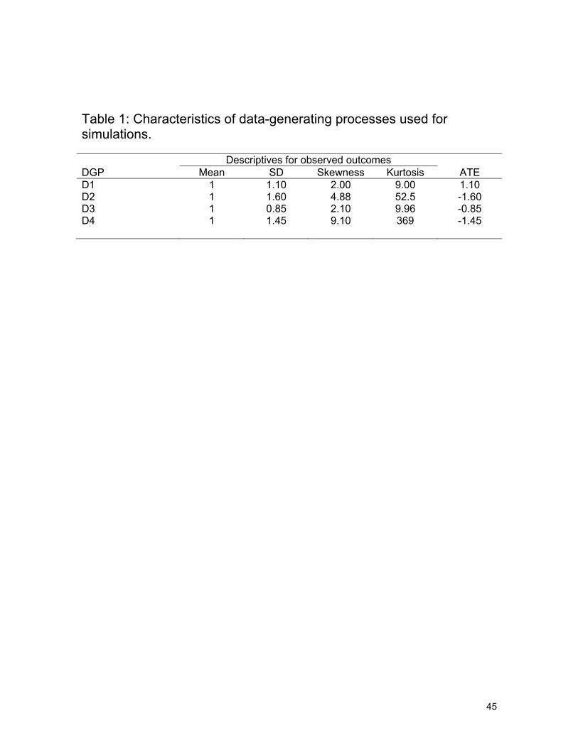
45

Table 1: Characteristics of data-generating processes used for simulations. Descriptives for observed outcomes DGP Mean SD Skewness Kurtosis ATE D1 1 1.10 2.00 9.00 1.10 D2 1 1.60 4.88 52.5 -1.60 D3 1 0.85 2.10 9.96 -0.85 D4 1 1.45 9.10 369 -1.45

46

Table 2: Estimated average treatment effect of BCSRT versus MST in breast cancer patients. Model: Estimator ATE (std. error) Difference from

ATE(EEE) C1: OLS 11,147 (1513) 1,164 (805)+

C2: log-link GLM 12,318 (1596) 2,335 (635)++

C3: EEE 9,983 (1350) - P1: Quintile-based PS 11,384 (1633) 1,401 (1389) P2: OLS-PS 10,869 (1546) 886 (1111) P3: IPW-PS 10,994 (2271) 1,011 (2151) P4a: OLS-DR 10,942 (2649) 959 (2492) P4b: log-GLM-DR 11,418 (1981) 1,435 (1752) P4c: EEE-DR 10,284 (1788) 301 (1350) Significant at: ++, 5%, +, 10%

47

Den

sity

.4 .5 .6 .7 .8 .9 1Estimated propensity scores

for D=1for D=0

Distribution of propensity scores by treatment groups

(a)

0.5

11.

52

2.5

.4 .5 .6 .7 .8 .9 1Estimated propensity Score

E(X1|D=0) E(X1|D=1)E(X2|D=0) E(X2|D=1)E(X3|D=0) E(X3|D=1)

(b)

0.1

.2.3

.4.5

.6

.4 .5 .6 .7 .8 .9 1Estimated propensity Score

SD(X1|D=0) SD(X1|D=1)SD(X2|D=0) SD(X2|D=1)SD(X3|D=0) SD(X3|D=1)

(c)

.3.2

.10

-.1-.2

-.3-.4

-.5-.6

-.7

.4 .5 .6 .7 .8 .9 1Estimated propensity Score

Corr(X1,X2|D=0) Corr(X1,X2|D=1)Corr(X1,X3|D=0) Corr(X1,X3|D=1)Corr(X2,X3|D=0) Corr(X2,X3|D=1)

(d) Figure 1: Initial Simulation Results (averaged over 1000 replicates): (a) Distribution of propensity scores by treatment groups; (b) Mean X’s by treatment status over estimated propensity score; (c) Std. Deviation of X’s by treatment status over estimated propensity score; (d) Correlation between X’s by treatment status over estimated propensity score.

48

Den

sitie

s

0 2 4 6 8 10Y (Scaled to have E(Y)=1)

DGP D1DGP D2DGP D3DGP D4

X-scale trucated at 10

Figure 2: Probability densities of Y under each data generating process, where Y was scaled so that E(Y) = 1in each case.

49

.91

.94

.9

.91

.911.91.95.9

.91

.911.9.93.9

.91

.94

.9

.91

.911.91.95.9

.91

.911.9.93.9

Regression Methods:C1: OLSC2: Log-GLMC3: EEE

PS & DR Methods (Sat.):P1: PS-QuintilesP2: PS-OLSP3: IPWP4a: OLS-DRP4b: Log-GLM-DRP4c: EEE-DR

PS & DR Methods (Unsat.):P1: PS-QuintilesP2: PS-OLSP3: IPWP4a: OLS-DRP4b: Log-GLM-DRP4c: EEE-DR

RRMSE RMAE

-150 -125 -100 -75 -50 -25 0 25 50 75 100 125 150% Bias

Sat.: Saturated PS estimator; Unsat.: Unsaturated PS estimator

(a)

.7

.65

.68

.64

.711.66..

.65

.75

.91

.67

.64

.73

.7

.65

.68

.64

.711.66..

.65

.75

.91

.67

.64

.73

Regression Methods:C1: OLSC2: Log-GLMC3: EEE

PS & DR Methods (Sat.):P1: PS-QuintilesP2: PS-OLSP3: IPWP4a: OLS-DRP4b: Log-GLM-DRP4c: EEE-DR

PS & DR Methods (Unsat.):P1: PS-QuintilesP2: PS-OLSP3: IPWP4a: OLS-DRP4b: Log-GLM-DRP4c: EEE-DR

RRMSE RMAE

-150 -125 -100 -75 -50 -25 0 25 50 75 100 125 150% Bias

Sat.: Saturated PS estimator; Unsat.: Unsaturated PS estimator

(b)

Figure 3: Simulation results on the %Bias and 95% CI in estimating ATE, ratio of Std. error of ATE and the ratio of RMSE between alternative estimators and IPW(Saturated model) estimator using (a) Data Generating Process D1 and (b) Data Generating Process D2.

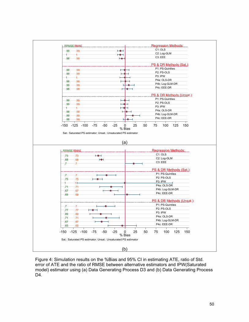
50

.991.98

.99

.991.98.99.98

.99

.991.98.99.98

.991.98

.99

.991.98.99.98

.99

.991.98.99.98

Regression Methods:C1: OLSC2: Log-GLMC3: EEE

PS & DR Methods (Sat.):P1: PS-QuintilesP2: PS-OLSP3: IPWP4a: OLS-DRP4b: Log-GLM-DRP4c: EEE-DR

PS & DR Methods (Unsat.):P1: PS-QuintilesP2: PS-OLSP3: IPWP4a: OLS-DRP4b: Log-GLM-DRP4c: EEE-DR

RRMSE RMAE

-150 -125 -100 -75 -50 -25 0 25 50 75 100 125 150% Bias

Sat.: Saturated PS estimator; Unsat.: Unsaturated PS estimator

(a)

.73

.68

.7

.7

.751.71.67.69

.7

.77

.89

.71

.67

.65

.73

.68

.7

.7

.751.71.67.69

.7

.77

.89

.71

.67

.65

Regression Methods:C1: OLSC2: Log-GLMC3: EEE

PS & DR Methods (Sat.):P1: PS-QuintilesP2: PS-OLSP3: IPWP4a: OLS-DRP4b: Log-GLM-DRP4c: EEE-DR

PS & DR Methods (Unsat.):P1: PS-QuintilesP2: PS-OLSP3: IPWP4a: OLS-DRP4b: Log-GLM-DRP4c: EEE-DR

RRMSE RMAE

-150 -125 -100 -75 -50 -25 0 25 50 75 100 125 150% Bias

Sat.: Saturated PS estimator; Unsat.: Unsaturated PS estimator

(b)

Figure 4: Simulation results on the %Bias and 95% CI in estimating ATE, ratio of Std. error of ATE and the ratio of RMSE between alternative estimators and IPW(Saturated model) estimator using (a) Data Generating Process D3 and (b) Data Generating Process D4.

51

% optimal: Data Generating Processes

DGP D1 DGP D2 DGP D3 DGP D4 Optimal Estimator EEE EEE OLS-PS Log-GLM-DR Methods EEE 43% 81% 7% 12% OLS-PS 39% 0% 89% 0% Log-GLM-DR 7% 0% 0% 46% IPW 11% 19% 4% 42% Figure 5: An algorithm to select optimal estimator (assumes that the initial regression run is the EEE model), w/i = within, nw/i = not within; and the percentage of simulated replicate datasets in which a method was found to be optimal following this algorithm.

52

0.1

.2.3

.4.5

.6.7

.8.9

1E

stim

ated

pro

pens

ity s

core

s

among BCSRT users among MST users

Propensity to choose BCSRT

(a)

-1.5

-1-.5

0.5

11.

52

2.5

3D

iffer

ence

s be

twee

n B

CS

RT

& M

ST

0 .1 .2 .3 .4 .5 .6 .7 .8 .9 1Estimated propensity Score

E(ChSc | BCSRT=1) - E(ChSc | BCSRT=0)SD(ChSc | BCSRT=1) - SD(ChSc | BCSRT=0)Corr(ChSc, HH_Inc | BCSRT=1) - Corr(ChSc, HH_Inc | BCSRT=0)

(b)

Figure 6: (a) Distribution of estimated propensity scores by treatment groups; (b) Imbalances in mean and standard deviation of Charlson Index score (ChSc) and the correlation between CHSc and median Household income between treatment groups at specific values (ranges in the case of correlation) of estimated propensity scores.

53

-15

-10

-50

510

%B

ias

0 2 4 6 8 10Deciles of Linear Predictors

OLSlog-GLMEEE

(a)

-15

-10

-50

510

%B

ias

0 2 4 6 8 10Deciles of Linear Predictors

OLS-PSOLS-DRlog-GLM-DREEE-DR

(b)

Figure 7: Analysis on cost of breast cancer treatments. Profile of residuals over the deciles of linear predictors for (a) OLS, log-GLM and EEE methods and (b) OLS=PS, OLS-DR, log-GLM-DR and the EEE-DR methods.