1

C o m p u t a b l e s c e n e s a n d s t r u c t u r e s i n F i l m s

Hari Sundaram and Shih-Fu Chang Email: {sundaram, sfchang}@ee.columbia.edu

Dept. Of Electrical Engineering, Columbia University,

New York, New York 10027.

Abstract

In this paper we present a computational scene model and also derive novel algorithms

for computing audio and visual scenes and within-scene structures in films. We begin by

mapping insights from film-making rules and experimental results from the psychology of

audition into a computational scene model. We define a visual computable scene to be a

segment that exhibits long-term consistency with regard to chromaticity and lighting. The

computable audio scene is a segment that exhibits long-term consistency with respect to

ambient sound. In our computational model, we derive four types of computable scenes that

arise due to different kinds of audio and video scene boundary synchronizations. Central to

the computational model is the notion of a causal, finite-memory viewer model. We segment

the audio and video data separately. In each case we determine the degree of correlation of

the most recent data in the memory with the past. The audio and video scene boundaries are

determined using local maxima and minima respectively. We show how to exploit the local

topology of an image sequence in conjunction with statistical tests, to determine dialogs. We

also derive a simple algorithm to detect silences in audio.

An important feature of our work is to introduce semantic constraints on our

computational model. This involves using silence and structural information to resolve

ambiguities in certain situations. This results in computable scenes that are more consistent

with human observations. The algorithms were tested on a difficult data set: three

commercial films. We take the first hour of data from each of the three films. The best

results: computational scene detection: 94% dialogue detection: 91% recall and 100%

precision.

2

1. Introduction

This paper deals with the problem of computing scenes, within films by fusing

information from audio and visual boundary detectors and visual structure. We also derive

algorithms for detecting visual structures in the film. The problem is important for several

reasons: (a) automatic scene segmentation is the first step towards greater semantic

understanding of the film (b) breaking up the film into scenes will help in creating film

summaries, thus enabling a non-linear navigation of the film. (c) the determination of visual

structure within each scene (e.g. dialogues), will help in the process of visualizing each scene

in the film summary. (d) in recent work, we have used these computable scenes in

conjunction with the idea of visual complexity for generating visual skims [25].

There has been prior work on video scene segmentation using image data alone [7] [30].

In [30], the authors derive scene transition graphs to determine scene boundaries. However,

cluster thresholds are difficult to set and must be manually tuned. In [7], the authors use a

infinite, non-causal memory model to segment the video. We use this idea of memory in our

current work, but in a finite, causal setting. Prior work [17] [19][22] concerning the problem

of audio segmentation dealt with very short-term (100 ms) changes in a few features (e.g.

energy, cepstra). This was done to classify the audio data into several predefined classes such

as speech, music ambient sounds etc. They do not examine the possibility of using the long-

term consistency found in the audio data for segmentation.

There has been some prior work on joint audio-visual segmentation [6] [10] [16]. In [6],

the authors, denote a scene change point to occur at a frame, which exhibits: (a) a shot cut

(b) an audio change and (c) a high motion change. However, these are short term

phenomena, and the they do not investigate long term correlations in either audio or video

data, or the relationship of these detectors to the presence of structure (e.g. dialogs). Also, by

focusing on synchronous audio visual events, they overlook the possibility of having single,

unsynchronized, but semantically important audio or visual events.

There has been some prior work that analyzed film data [5] [12]. In [5], the authors use

visual features alone to determine a logical story unit (LSU): a collection of temporally

interrelated events. The LSU is detected using a single link clustering algorithm with cluster

thresholds that change with the content of the cluster. The is done on the shots while

3

ignoring the duration. However, importantly, the duration of a scene can vary greatly with

directorial style and semantics. In [12], the authors aim at automating the process of creating

video abstracts, given a time budget, not segmentation. Neither of these works attempts to

incorporate film-making constraints on the minimum number of shots in a scene, dialogs, or

examines the inter-relationships between audio and video scene boundaries.

There has been prior work on structure detection [30], [31]. There, the authors begin

with time-constrained clusters of shots and assign labels to each shot. Then, by analyzing the

label sequence, they determine the presence of dialogue. This method critically depends

upon cluster threshold parameters that need to be manually tuned.

There are constraints on what we see and hear in films, due to rules governing camera

placement, continuity in lighting as well as due to the psychology of audition. In this paper,

we develop notions of a video and audio computable scenes by making use of these

constraints. A video computable scene (v-scene) exhibits long-term consistency with respect

to two properties: (a) chromatic composition of the scene (b) lighting conditions. The audio

computable scene (a-scene) exhibits long-terms consistency with respect to the ambient

audio. We derive four types of

computable scenes (c-scene) that

arise from different forms of

synchronizations between a-

scene and v-scene boundaries.

We term these scenes as

computable, since they can be

reliably computed using low-

level features alone. In this

paper, we do not deal with the

semantics of a scene. Instead, we

focus on the idea of determining

a computable scene, which we

believe is the first step in

deciphering the semantics of a

scene.

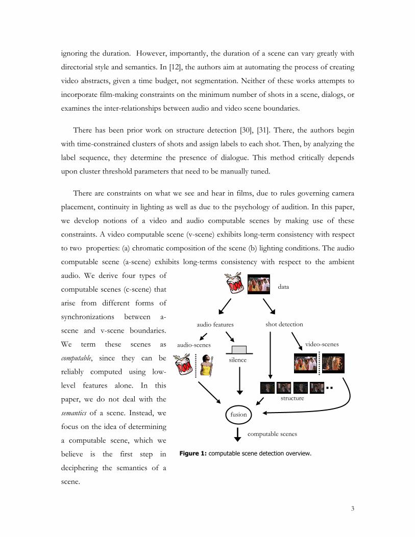
Figure 1: computable scene detection overview.

silence

structure

fusion

computable scenes

audio-scenes video-scenes

audio features shot detection

data

4

We present algorithms for determining computable scenes and periodic structures that

may exist within such scenes. We extend the memory model found in [7], to cover both

audio and video data. Secondly, we make our memory model causal and finite. The model

has two parameters: (a) an analysis window that stores the most recent data (the attention

span) (b) the total amount of data (memory). In order to segment the data into audio scenes,

we compute correlations amongst the audio features in the attention-span with the data in

the rest of the memory. The video data comprises shot key-frames. The key-frames in the

attention span are compared to the rest of the data in the memory to determine a coherence

value. This value is derived from a color-histogram dissimilarity. The comparison takes also

into account the relative shot length and the time separation between the two shots. We

local maxima and minima respectively, to determine scene change points.

We introduce a topological framework that examines the local metric relationships

between images for structure detection. Since structures (e.g. dialogs) are independent of the

duration of the shots, we can detect them independent of the v-scene detection framework.

We exploit specific local structure to compute a function that we term the periodic analysis

transform. We test for significant dialogs using the standard Students t-test. The silence is

detected via a threshold on the average energy; we also impose minimum duration

constraints on the detector.

A key feature of our work is the idea of imposing semantic constraints on our

computable scene model. This involves fusing (see figure 1) results from silence and

structure detection algorithms. The computational model cannot disambiguate between

these two cases involving two long and widely differing shots: (a) in a dialog sequence and

(b) adjoining video scenes. However, human beings recognize the structure in the sequence

and thus group the dialog shots together. Silence is useful in two contexts: (a) detecting the

start of conversation by determining significant pauses [4] and (b) in English films, the

transitions between computable scenes may involve silence. Our experiments show that the

c-scene change detector and the structure detection algorithm works well.

The rest of this paper is organized as follows. In the next section, we formalize the

definition of a computable scene. In section 3, we present our memory model. In sections 4

we discuss techniques to determine video scene boundaries. In section 5, we discuss our

5

topological framework for determining visual structure while in section 6, we discuss audio

scene boundary detection. In section 7, we discuss our technique to merge information from

audio, video scene boundaries, structure detection and silences. In sections 8 and 9 we

present our experimental results and a discussion on possible model breakdowns. Finally, in

section 10, we present our conclusions.

2. What is a computable scene?

In this section we shall define the notion of a computable scene. We begin with a few

insights obtained from understanding the process of film-making and from the psychology

of audition. We shall use these insights in creating our computational model of the scene.

2.1. Insights from Film Making Techniques

The line of interest is an imaginary line drawn by

the director in the physical setting of a scene [3].

During the filming of the scene, all the cameras are

placed on one side of this line (also referred to as the

180 degree rule). This is because we desire successive

shots to maintain the spatial arrangements between the

characters and other objects in the location1. The 180

degree rule has interesting implications on the

computational model of the scene. Since all the

cameras in the scene remain on the same side of the

line in all the shots, there is an overlap in the field of

view of the cameras (see figure 2). This implies that there will be a consistency to the

chromatic composition and the lighting in all the shots. Film-makers also seek to maintain

continuity in lighting amongst shots within the same physical location. This is done even

when the shots are filmed over several days. This is because viewers perceive the change in

lighting as indicative of the passage of time. For example, if two characters are shown talking

in one shot, in daylight, the next shot cannot show them talking at the same location, at

night.

1 This is so infrequent that directors who transgress the rule are noted in the film theory community. e.g. Alfred Hitchcock�s willful violation in a scene in his film North by Northwest [3].

Figure 2: showing the line of interest (thick dashed line) in a scene. We also see the fields-of-view of the two cameras intersecting.

6

2.2. The Psychology of Audition

The term auditory scene analysis was coined by Bregman in his seminal work on auditory

organization [1]. In his psychological experiments on the process of audition, Bregman made

many interesting observations, a few of which are reproduced below:

• Unrelated sounds seldom begin and end at the same time.

• A sequence of sounds from the same source seem to change its properties smoothly and

gradually over a period of time. The auditory system will treat the sudden change in

properties as the onset of a new sound.

• Changes that take place in an acoustic event will affect all components of the resulting

sound in the same way and at the same time. For example, if we are walking away from

the sound of a bell being struck repeatedly, the amplitude of all the harmonics will

diminish gradually. At the same time, the harmonic relationships and common onset2 are

unchanged.

Bregman also noted that different auditory cues (i.e. harmonicity, common-onset etc.)

compete for the user�s attention and depending upon the context and the knowledge of the

user, will result in different perceptions. Different computational models (e.g. [2]) have

emerged in response to those experimental observations. While these models differ in their

implementations and differ considerably in the physiological cues used, they focus on short-

term grouping strategies of sound. Notably, Bregman�s observations indicate that long-term

grouping strategies are also used by human beings (e.g. it is easy for us to identify a series of

footsteps as coming from one source) to group sound.

2.3. The Computable Scene Model

The constraints imposed by production rules in film and the psychological process of

hearing lead us to the following definition of audio and video scenes. A video scene is a

continuous segment of visual data that shows long-term3 consistency with respect to two

2 Different sounds emerging from a single source begin at the same time. 3 Analysis of experimental data (one hour each, from five different films) indicates that for both the audio and the video scene, a minimum of 8 seconds is required to establish context. These scenes are in the usually same location (e.g. in a room, in the marketplace etc.) are and are typically 40~50 seconds long.

7

properties: (a) chromaticity and (b) lighting conditions, while an audio scene exhibits a long

terms consistency with respect to ambient sound. We denote them to be computable since

these properties can be reliably and automatically determined using low-level features present

in the audio-visual data. The a-scene and the v-scenes represent elementary, homogeneous

chunks of information. We define a computable scene (abbreviated as c-scene) in terms of

the relationships between a-scene and v-scene boundaries. It is defined to be a segment

between two consecutive, synchronized4 audio visual scenes. This results in four cases of

interest5 (Table 1).

Table 1: The four types of c-scenes that exist between consecutive, synchronized audio-visual changes. solid circles: indicate audio scene boundaries, triangles indicate video scene boundaries

Type Abbr. Figure

Pure, no audio

or visual

change present.

P

Audio changes

consistent

visual.

Ac-V

Video changes

but consistent

audio.

A-Vc

Mixed mode:

contains

unsynchronized

audio and

visual scene

boundaries.

MM

4 In films, audio and visual scene changes will not exactly occur at the same time, since this is disconcerting to the audience. They make the audio flow �over the cut� by a few seconds [15], [18]. 5 Note that the figures for Ac_v, A-Vc and MM, in Table 1 show only one audio/visual change. Clearly, multiple changes are possible. We show only one change for the sake of figure clarity.

8

We validated the computable scene definition, which appeared out of intuitive

considerations, with actual film data. The data were from three one hour segments from

three English language films6. The definition for a scene works very well in many film

segments. In most cases, the c-scenes are usually a collection of shots that are filmed in the

same location and time and under similar lighting

conditions (these are the P and the Ac-V scenes).

The A-Vc (consistent audio, visuals change)

scenes seem to occur under two circumstances.

In the first case, the camera placement rules

discussed in section 2.1 are violated. These are

montage7 sequences and are characterized by

widely different visuals (differences in location,

time of creation as well as lighting conditions) which create a unity of theme by manner in

which they have been juxtaposed. Mtv videos are good examples of such scenes. The second

case consists of a sequence of v-scenes that individually obey the camera placement rules

(and hence each have consistent chromaticity and lighting). We refer to the second class as

transient scenes. Typically, transient scenes can occur when the director wants to show the

passage of time e.g. a scene showing a journey, characterized by consistent audio track.

Mixed mode (MM) scenes far less frequent, and can for example occur, when the

director continues an audio theme well into the next v-scene, in order to establish a

particular semantic feeling (joy/sadness etc.). Table 2 shows the c-scene type break-up from

the first hour of the film Sense and Sensibility. There were 642 shots detected in the video

segment. The statistics from the other films are similar. Clearly, c-scenes provide a high

degree of abstraction, that will be extremely useful in generating video summaries. Note that

while this paper focuses on computability, there are some implicit semantics in our model:

the P and the Ac-V scenes, that represent c-scenes with consistent chromaticity and lighting

are almost certainly scenes shot in the same location.

6 The English films: Sense and Sensibility, Pulp Fiction, Four Weddings and a Funeral. 7 In classic Russian montage, the sequence of shots are constructed from placing shots together that have no immediate similarity in meaning. For example, a shot of a couple may be followed by shots of two parrots kissing each other etc. The meaning is derived from the way the sequence is arranged.

C-scene breakup Count Fraction

Pure 33 65%

Ac-V 11 21%

A-Vc 5 10%

MM 2 4%

Total 51 100%

Table 2: c-scene breakup from the film sense and sensibility.

9

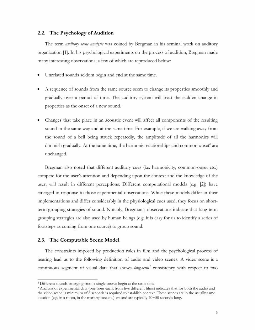
3. The Memory Model

In order to segment data into scenes, we use a causal, first-in-first-out (FIFO) model of

memory (figure 3). This model is derived in part from the idea of coherence [7]. In our

model of a listener, two parameters are of interest: (a) memory: this is the net amount of

information (Tm) with the viewer and (b) attention span: it is the most recent data (Tas) in the

memory of the listener. This data is used by the listener to compare against the contents of

the memory in order to decide if a scene change has occurred.

The work in [7] dealt with a non-causal, infinite memory model based on psychophysical

principles, for video scene change detection. We use the same psychophysical principles to

come up with a causal and finite memory model. Intuitively, causality and a finite memory

will more faithfully mimic the human memory-model than an infinite model. We shall use

this model for both audio and video scene

change detection.

The next three sections deal with our

core framework. In the next section we

shall discuss our video scene boundary

detection algorithm, and follow that with a

section on structure detection. In section 6, we discuss audio scene boundary and silence

detection. Finally in section 7, we discuss the challenging task of fusing the information

obtained in the prior sections, to determine computable scene boundaries as well as

detecting unsynchronized a-scene and v-scene boundaries.

4. Determining Video Scene boundaries

In this section, we shall describe the algorithm for v-scene boundary detection. The

algorithm is based on notions of recall and coherence. We model the v-scene as a contiguous

segment of visual data that is chromatically coherent and also possesses similar lighting

conditions. A v-scene boundary is said to occur when there is a change in the long-term

chromaticity and lighting properties in the video. This stems from the film-making

constraints discussed in section 2.1.

time

to attention span

memory Tm

Tas Figure 3: The attention span Tas is the most recent data in the memory. The memory (Tm) is the size of the entire buffer.

10

The framework that we propose, can conceptually work without having to detect shots,

i.e. with raw frames alone. However, this would lead to an enormous increase in the

computational complexity of the algorithm. Hence, the video stream is converted into a

sequence of shots using a simple color and motion based shot boundary detection algorithm

[9], that produces segments that have predictable motion and consistent chromaticity. A

frame at a fixed time after the shot boundary is extracted and denoted to be the key-frame.

4.1. Recall

In our visual memory model, the data is in the form of key-frames of shots (figure 4) and

each shot occupies a definite span of time. The model also allows for the most recent and

the oldest shots to be partially present in the buffer. A point in time (to) is defined to be a

scene transition boundary if the shots that come after that point in time, do not recall [7]

the shots prior to that point. The idea of recall between two shots a and b is formalized as

follows:

( , ) (1 ( , )) (1 / ),a b mR a b d a b f f t T= − • • • − ∆ <1>

where, R(a,b) is the recall between

the two shots a, b. d(a,b) is a L1 color-

histogram based distance between the

key-frames corresponding to the two

shots, fi is the ratio of the length of

shot i to the memory size (Tm). ∆t is

the time difference between the two

shots. The formula for recall indicates

that recall is proportional to the

length of each of the shots. This is

intuitive since if a shot is in memory

for a long period of time it will be

recalled more easily. Again, the recall

between the two shots should

decrease if they are further apart in time.

Figure 4: (a) Each solid colored block represents a single shot. (b) each shot is broken up into �shot-lets� each at most δ sec. long. (c) the bracketed shots are present in the memory and the attention span. Note that sometimes, only fractions of shots are present in the memory.

time

time

each shot is broken up into δ sec. long �shot-lets.�

to attention

memory Tm

Tas

time

(a)

(b)

(c)

11

We need to introduce the notion of a �shot-let.� A shot-let is a fraction of a shot,

obtained by breaking individual shots into δ sec. long chunks but could be smaller due to

shot boundary conditions. Each shot-let is associated with a single shot and its representative

frame is the key-frame corresponding to the shot. In our experiments, we find that δ = 1

sec. works well. Figure 4 shows how shot-lets are constructed. The formula for recall for

shot-lets is identical to that for shots.

4.2. Computing Coherence

Coherence is easily defined using the definition of recall:

max{ \ }

( ) ( , ) ( )as m as

o oa T b T T

C t R a b C t∈ ∈

=

∑ ∑ <2>

where, C(to) is the coherence across the boundary at to and is just the sum of recall values

between all pairs of shot-lets across the boundary at to. Cmax(to) is obtained by setting

d(a,b)=0 in the formula for recall (equation <1>) and re-evaluating the numerator of

equation <2>. This normalization compensates for the different number of shots in the

buffer at different instants of time. Note that shot-lets essentially fine-sample the coherence

function while preserving shot boundaries.

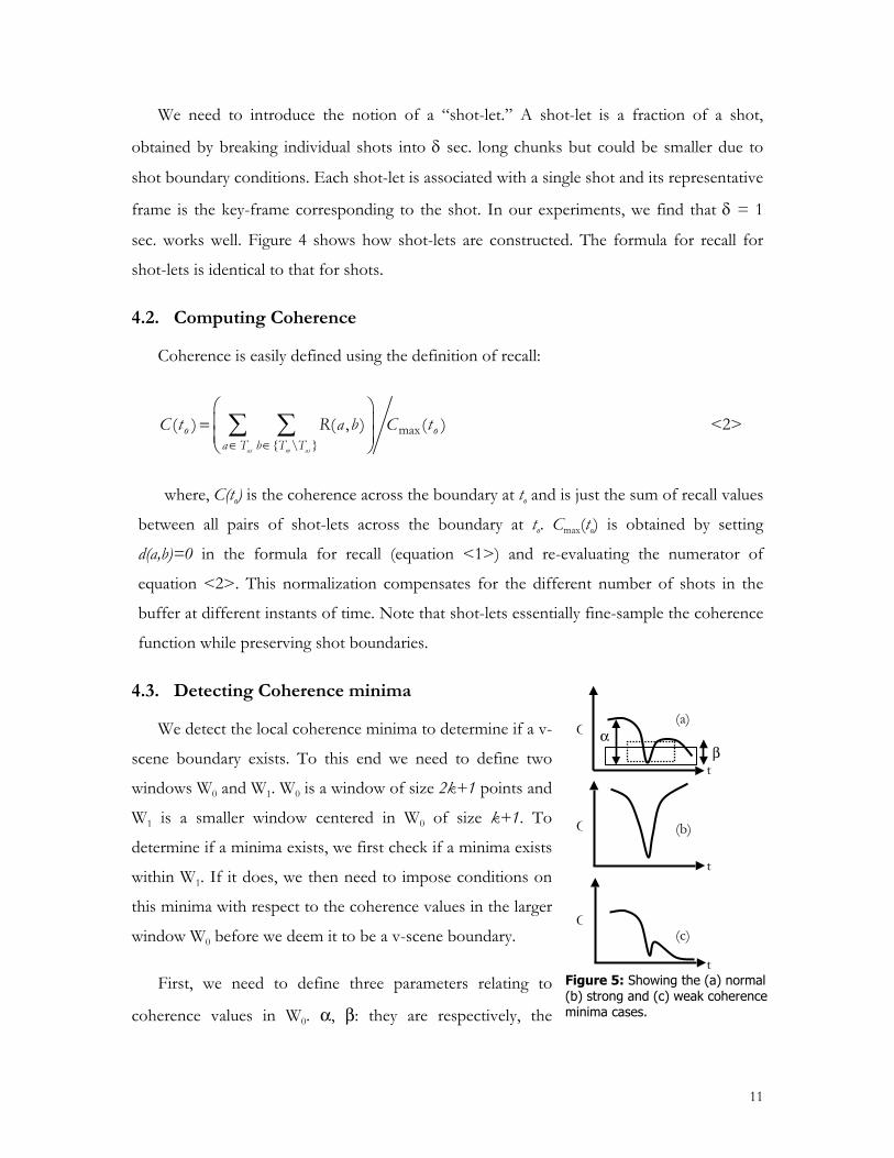
4.3. Detecting Coherence minima

We detect the local coherence minima to determine if a v-

scene boundary exists. To this end we need to define two

windows W0 and W1. W0 is a window of size 2k+1 points and

W1 is a smaller window centered in W0 of size k+1. To

determine if a minima exists, we first check if a minima exists

within W1. If it does, we then need to impose conditions on

this minima with respect to the coherence values in the larger

window W0 before we deem it to be a v-scene boundary.

First, we need to define three parameters relating to

coherence values in W0. a, b: they are respectively, the

Figure 5: Showing the (a) normal (b) strong and (c) weak coherence minima cases.

b t

C

t

C

t

C

(a)

(b)

(c)

a

12

difference between the maxima in the left and right half coherence windows and the minima

value. d : this is the difference between the minima and the global minima in W0. Then, on

the basis of these three values, we classify the minima into three categories (see figure 5):

1. Strong : min( , ) 0.3 ( min( , ) 0.1 max( , ) 0.4 )S α β α β α β≡ > ∨ > ∧ >

2. Normal: (max( ) 0.1) (min( ) 0.05) ( 0.1) ( )N Sα β α β δ≡ , > ∧ , > ∧ < ∧ ¬

3. Weak : max( , ) 0.1 ( ) ( )W S Nα β≡ > ∧ ¬ ∧ ¬

The two window technique helps us detect the weak minima cases. The strong case is

good indicator a v-scene boundary between two highly chromatically dissimilar scenes. The

weak case becomes important when we have a transition from a chromatically consistent

scene to a scene which is not as consistent. These are the P Æ A-Vc, or Ac-V Æ A-Vc (and

vice-versa) type scene transitions (see Table 1). These categories become very useful when

we are fusing information from a-scene boundary detection, v-scene boundary detection,

silence detection and structure analysis.

5. Computing Visual Structure

In this section, we shall give an overview of some of the possible structures that exist in

video sequences, an abstract representational technique and an algorithm for computing

dialogs. The analysis that follows assumes that the video data has been segmented into shots

and that each shot is represented by a single key-frame. We use a shot detector that uses

color coherence and predictable motion to do shot boundary detection [9].

Structures (e.g. dialogs) contain important semantic information, and also provide

complimentary information necessary to resolve v-scene boundaries. For example, in a

dialog that contains very long shots (say 25 sec. each) showing very different backgrounds,

the algorithm in section 4.2 will generate v-scene boundaries after each shot.

Computationally, this situation is no different from two long shots from completely

chromatically different (but adjacent) v-scenes. Human beings easily resolve this problem by

not only inferring the semantics from the dialogue, but also by recognizing the dialog

structure and grouping the shots contained in it into one semantic unit.

13

5.1. The Topology of Shots

Structures in video shot sequences, have an important property that the structure is

independent of the individual shot lengths. It is the topology (i.e. the metric relationships

between shots, independent of the duration of the shots) of the shots that uniquely

characterizes the structure. For example, in a dialog sequence (A-B-A-B-..), the lengths of

each shot will vary over the course of the dialog, and in general are related to: (a) the

semantics of the dialog, (b) the presence of one speaker to who may dominate and (c)

relationship dynamics between the speakers i.e. the dominant speaker may change over the

course of the conversation. We now introduce the idea of the topological graph, central to

all our structure detection algorithms.

5.2. The Topological graph

Let S = {I, d} be the metric space induced by the set of all images I in the video

sequence by the distance function d. The topological graph TG = {V,E} of a sequence of k

images, is a fully connected graph, with the images at the vertices and where the edges

specify the metric relationship between the images. The graph has associated with it, the

topological matrix TM, which is the k by k matrix where TM(i,j) contains the value of the

edge connecting node i to node j in the graph. For an idealized dialog sequence of 6 images

(A-B-A-B-A-B), with d(A,B) = 1, we would get the following topological matrix:

0 1 0 1 0 11 0 1 0 1 00 1 0 1 0 11 0 1 0 1 00 1 0 1 0 11 0 1 0 1 0

<3>

The idea of the topological graph is distinct from the scene transition graph [30][31].

There, the authors cluster shots, and examine relationships between these clusters to

determine scene change points as well as dialogs. Here, we are strictly interested in the

topological property of a sequence of images and not in determining scene transitions.

14

5.3. Topological Structures

We investigate two structures in this work: the regular anchor and the dialog. However,

for sake of brevity, we shall only present our dialog detection algorithm here. The details on

the detection of regular anchors (computed using random permutations on the idealized

topological matrix) and a more details on topological sequences can be found in [27].

Regular Anchors: A five image length regular

anchor sequence is as follows: A-I1-A-I2-A,

where, A is the anchor, and I1 and I2 can be

arbitrary images. The idealized topological

relationship is then: d(A,I1) = d(A,I2) = 1; and

since we don�t care about the relationship between I1 and I2, we specify the edge (and the

corresponding entry in the topological matrix) between the nodes representing I1 and I2 in

TG as -1. The extension to an odd8 (2N+1) sequence immediately follows. A three image

regular anchor is shown in figure 6.

Dialogs: A six image length dialog A-B-A-B-A-

B, is completely specified with the following

idealized topological relationship: d(A,B) = 1.

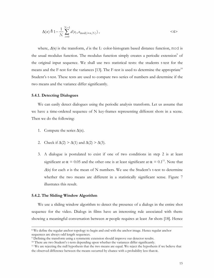
5.4. Detecting Dialogs

A dialog has a specific local topological

property: every 2nd frame is alike while adjacent

frames differ (figure 7). In the idealized

topological matrix for the dialog (equation <3>

), this appears as the 1st off-diagonal being all

ones, the 2nd off-diagonal being all zeros and

the 3rd off-diagonal being all ones. Hence we

need to define a periodic analysis transform to estimate existence of this pattern in a

sequence of N shot key-frames. Let oi where i ∈{0,N-1} be a time ordered sequence of

images. Then:

�

Figure 7: A dialogue scene and its corresponding periodic analysis transform. Note the distinct peaks at n = 2, 4 . . .

Figure 6: A three image regular anchor.

15

1

mod( , )0

1( ) 1 ( , )N

i i n Ni

n d o oN

−

+=

∆ − ∑! , <4>

where, ∆(n) is the transform, d is the L1 color-histogram based distance function, mod is

the usual modulus function. The modulus function simply creates a periodic extension9 of

the original input sequence. We shall use two statistical tests: the students t-test for the

means and the F-test for the variances [13]. The F-test is used to determine the appropriate10

Student�s t-test. These tests are used to compare two series of numbers and determine if the

two means and the variance differ significantly.

5.4.1. Detecting Dialogues

We can easily detect dialogues using the periodic analysis transform. Let us assume that

we have a time-ordered sequence of N key-frames representing different shots in a scene.

Then we do the following:

1. Compute the series ∆(n).

2. Check if ∆(2) > ∆(1) and ∆(2) > ∆(3).

3. A dialogue is postulated to exist if one of two conditions in step 2 is at least

significant at α = 0.05 and the other one is at least significant at α = 0.111. Note that

∆(n) for each n is the mean of N numbers. We use the Student�s t-test to determine

whether the two means are different in a statistically significant sense. Figure 7

illustrates this result.

5.4.2. The Sliding Window Algorithm

We use a sliding window algorithm to detect the presence of a dialogs in the entire shot

sequence for the video. Dialogs in films have an interesting rule associated with them:

showing a meaningful conversation between m people requires at least 3m shots [18]. Hence

8 We define the regular anchor topology to begin and end with the anchor image. Hence regular anchor sequences are always odd length sequences. 9 Defining the transform using a symmetric extension should improve our detector results. 10 There are two Student�s t-tests depending upon whether the variances differ significantly. 11 We are rejecting the null hypothesis that the two means are equal. We reject the hypothesis if we believe that the observed difference between the means occurred by chance with a probability less than α.

16

in a dialogue that shows two participants, this implies that we must have a minimum of six

shots. As a consequence, we analyze six frames at a time starting with the first shot key-

frame. The algorithm is as follows:

1. Run the dialogue detector on the current window.

2. If no dialogue is detected, keep shifting the window to the right by one key-frame to

the immediate right until either a dialogue has been detected or we have reached the

end of the video sequence.

3. If a dialogue has been detected, keep shifting the starting point of the window by

two key-frames, until we no longer have a statistically significant dialog or if we

reached the end of the video sequence.

4. Merge all the overlapping dialog sequences just detected.

5. Move the starting point of the window to be the first frame after the last frame of

the last successful dialog.

The sliding window algorithm can sometimes �overshoot� and �undershoot.� i.e. it can

include a frame before (or after) as being part of the dialog. These errors are eliminated by

simply checking if the local dialog topological property holds at the boundaries. If not, we

simply drop those frames. This results in an algorithm that generates statistically significant

dialogs, with precise begin and end locations.

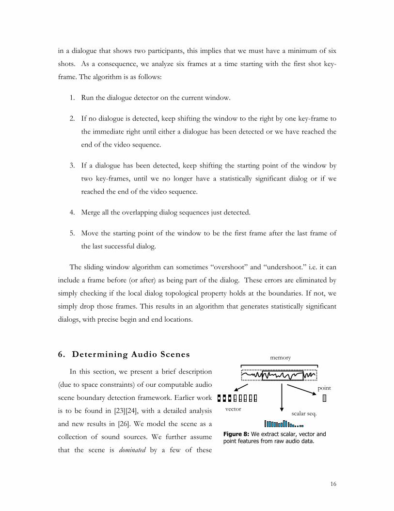
6. Determining Audio Scenes

In this section, we present a brief description

(due to space constraints) of our computable audio

scene boundary detection framework. Earlier work

is to be found in [23][24], with a detailed analysis

and new results in [26]. We model the scene as a

collection of sound sources. We further assume

that the scene is dominated by a few of these

Figure 8: We extract scalar, vector and point features from raw audio data.

vector

memory

point

scalar seq.

17

sources. These dominant sources are assumed to possess stationary properties that can be

characterized using a few features. For example, if we are walking away from a tolling of a

bell, the envelope of the energy of the sound of the bell will decay quadratically. A scene

change is said to occur when the majority of the dominant sources in the sound change.

We model the audio data using three types of features: scalar sequences, vector

sequences and single points (figure 8). Features ([14], [17], [21], [23], [31]) are extracted per

section of the memory, and each section is Tas sec. long (the length of the attention span).

We use six scalar features: (1) zero-crossing rate, (2) spectral flux, (3) cepstral flux, (4) energy,

(5) energy variance (6) the low energy fraction. We determine three vector features: (1)

cepstral vectors (2) multi-channel cochlear decomposition (3) mel-frequency cepstral

coefficients. We also compute two point features: (1) spectral roll off point and (2) variance

of the zero crossing rate. The point features are called so because, just one value is obtained

for the duration of the entire attention span. All other features (except for the low-energy

fraction and the energy variance, which are computed per second), are obtained per 100ms

frame of the attention span. The cochlear decomposition was used because it was based on a

psychophysical ear model. The cepstral features are known to be good discriminators [14].

All the other features were used for their ability to distinguish between speech and music

[17], [21], [31]. The scalar sequence of feature values are modeled to consist of three parts: a

trend (in order to incorporate Bregman�s constraints) , a set of periodic components and

noise.

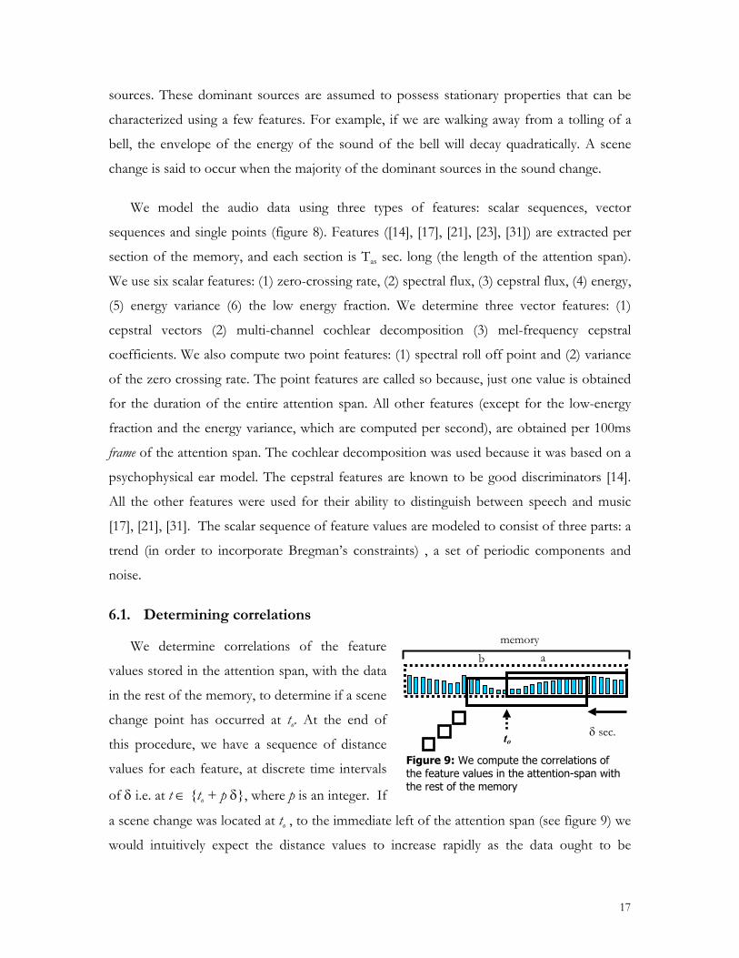
6.1. Determining correlations

We determine correlations of the feature

values stored in the attention span, with the data

in the rest of the memory, to determine if a scene

change point has occurred at to. At the end of

this procedure, we have a sequence of distance

values for each feature, at discrete time intervals

of δ i.e. at t ∈ {to + p δ}, where p is an integer. If

a scene change was located at to , to the immediate left of the attention span (see figure 9) we

would intuitively expect the distance values to increase rapidly as the data ought to be

Figure 9: We compute the correlations of the feature values in the attention-span with the rest of the memory

a memory

b

δ sec.to

18

dissimilar across scenes. We then compute β, the rate of increase of the distance at time t = 0.

The local maxima of the distance increase rate estimate β, represents the scene change

location point as estimated by that feature. Finally, we use a voting procedure amongst the

features, to determine scene change location points.

6.2. Determining Silences

Silences become particularly useful in detecting c-scene boundaries where v-scene

boundary occurs in a relatively silent section. There are two forms of silence in speech [21]:

within phrase silences and between phrase silences. The within phrase silences are due to

weak unvoiced sounds like /f/ or /th/ or weak voiced sounds such as /v/ or /m/.

However, such silences are short usually 20~150 ms long. In [21], the author uses a two class

classifier using Gaussian models for each pause class, to come up with a threshold of 165ms.

However, others have used a threshold of 647 ms [4], for distinguishing significant pauses.

In our experiments we detect silences greater than 500ms duration [26].

6.3. Determining weak a-scene boundaries

We now define the notion of a weak a-scene boundary. This is useful when determining

the rules for c-scene detection. A weak a-scene boundary has a significant amount of silence

at the boundary. We make further distinctions based on the amount of silence present.

• Compute the fraction of silence in a symmetric window (2WAS sec. long) around the

a-scene boundary. Let LAS and RAS be the left and right silence fractions. i.e. the

amount of silence in the left and right windows. Using the computed values of LAS

and RAS, we make the following distinctions:

o Pure Silence: ,min( ) 1.a AS ASF L R≡ = ,

o Silent: max( , ) 1.AS ASS L R≡ =

o Conversation:

≡ = ∧ > ∧ ¬min( , ) 0 max( , ) 0.125 ( ).p AS AS AS ASC L R L R S This is

just a test of significant silence in speech (ref. section 6.2).

19

7. Integrating Audio, Silence, Video and Structure

In this section we discuss our algorithm (figure 1 shows system overview) to integrate

information from the a-scene, v-scene boundary detection algorithms with the results of the

structure and silence detection algorithms. The computational scene model in Table 1, can

generate c-scenes that run counter to grouping rules that human beings routinely use. Hence,

the use of silence and structure detection imposes additional semantic constraints on the c-

scene boundary detection algorithm.

7.1. Detecting c-scenes

There are three principal rules for detecting c-scenes:

1. We detect a c-scene whenever we can associate a v-scene with an a-scene that lies

within a window of WC sec.

2. We declare a c-scene to be present when normal v-scenes (see section 4.3)

intersect silent regions.

3. We always associate a c-scene boundary with strong v-scene boundary locations.

The first rule is the synchronization rule for detecting c-scenes. The window WC is

necessary as film directors deliberately do not exactly align a-scene and v-scene boundaries;

at a perceptual level, this causes a smoother transition between scenes. There are some

exceptions to this rule, which we discuss later in the section. The second rule is important as

many transitions between c-scenes are silent (e.g. the first scene ends in silence and then the

second scene shows conversation, which also begins with silence). In such cases, audio scene

boundaries may not exist within WC sec. of the v-scene.

The third rule becomes necessary when there is no detectable a-scene boundary within

WC sec. of a strong v-scene boundary. Strong v-scene boundaries occur as transitions

between two v-scenes that are long in duration, and which differ greatly in chromatic

composition. Consider the following example. Alice and Bob are shown having

conversation. Towards the end of the scene, the director introduces background music to

emphasize a certain emotion. Then, the music is held over to the next scene for a few

seconds to maintain continuity. Note that in this case, there is no a-scene boundary near the

20

Figure 11: Remove a-scenes, v-scenes and detected silence, when present in structured sequences.

v-scene boundary, nor is there a silent region near the v-scene boundary. The notation used

in the figures in this section: silence: gray box, structure: patterned box, solid dot: a-scene

boundary, equilateral triangle: v-scene, solid right angled triangle: weak v-scene. Now, we

detail the steps in the algorithm.

Step 1: Remove v-scene or a-scene changes or silence

within structured sequences (i.e. within dialogs and regular

anchors) (figure 10.1). This is intuitive since human beings

recognize and group structured sequences into one

semantic unit.

Step 2: Place c-scene boundaries at strong (see section 4.3) v-scene boundaries. Remove all

strong v-scenes from the list of v-scenes.

Step 3: If an a-scene lies within WC sec. of a v-scene, place a c-scene boundary at the v-scene

location. However, there are three exceptions:

1. Do not associate a weak v-scene with a weak a-

scene.

2. If the v-scene is weak, it must synchronize with a

non-weak a-scene that is within WC/2 sec. i.e. we

have tighter synchronization requirements

for weak v-scenes.

3. Do not associate a normal v-scene with a

weak a-scene marked as silent (see section

6.3).

Step 4: Non-weak (see section 4.3) v-scene boundaries (i.e.

normal boundaries. Note that strong boundaries would have

already been handled in step 2) that intersect silent regions

are labeled as c-scene boundaries (figure 13). To determine

whether a v-scene boundary intersects silence, we do the

t

C

Figure 13: Non-weak coherence minimum intersecting silences (gray boxes) causes a c-scene boundary.

Figure 12: Do not associate normal v-scenes with a-scenes marked as silent.

Figure 11: Tight synchronization between weak v-scenes and non-weak a-scenes.

21

following:

• Compute the fraction of silence in a symmetric window (2WVS sec. long) around the

v-scene boundary. Let LVS and RVS be the left and right silence fractions. i.e. the

amount of data in the left and right windows that constitute silence.

• Then, declare a c-scene boundary if: 0.8 0.8VS VSL R> ∨ >

Now, we have a list of c-scenes, as well as lists of singleton video and audio scene

boundaries. The c-scenes are then post-processed to check if additional structure is present.

7.2. Post-processing c-scenes

Once we have detected all the c-scenes, we use a conservative post-processing rule to

eliminate false alarms. An irregular anchor shot in a semantic scene is a shot that the director

comes back to repeatedly, but not in a regular pattern, within the duration of the semantic

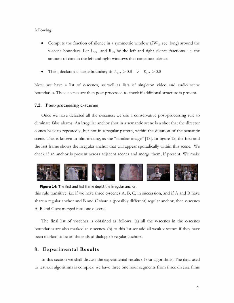
scene. This is known in film-making, as the �familiar-image� [18]. In figure 12, the first and

the last frame shows the irregular anchor that will appear sporadically within this scene. We

check if an anchor is present across adjacent scenes and merge them, if present. We make

this rule transitive: i.e. if we have three c-scenes A, B, C, in succession, and if A and B have

share a regular anchor and B and C share a (possibly different) regular anchor, then c-scenes

A, B and C are merged into one c-scene.

The final list of v-scenes is obtained as follows: (a) all the v-scenes in the c-scenes

boundaries are also marked as v-scenes. (b) to this list we add all weak v-scenes if they have

been marked to be on the ends of dialogs or regular anchors.

8. Experimental Results

In this section we shall discuss the experimental results of our algorithms. The data used

to test our algorithms is complex: we have three one hour segments from three diverse films

Figure 14: The first and last frame depict the irregular anchor.

22

in English: (a) Sense and Sensibility (b) Pulp Fiction and (c) Four Weddings and a Funeral. We begin

with a section that explains how the labeling of the ground truth data was done. It is

followed by sections on c-scene boundary detection and structure detection.

8.1. Labeling the Ground Truth

The audio and the video data were labeled separately (i.e. label audio without watching

the video and label video without hearing the audio). This was because when we use both the

audio and the video (i.e. normal viewing of the film) we tend to label scene boundaries

based on the semantics of the scene. Only one person (the first author) labeled the data.

apart. Due to space constraints, we summarize our labeling procedure.

We attempt to label the audio and video data into coherent segments. From empirical

observations of film data, it became apparent that for a group of shots to establish an

independent context, it must last at least 8 sec. Hence all the v-scenes that we label must last

more than 8 sec. We also set the minimum duration of an a-scene to be 8 sec. Then, the

labeling criteria were as follows: (a) do not mark v-scene boundaries in the middle of dialogs

or regular anchors, instead mark structure detection points at the beginning and end of the

dialogs/regular anchors. (b) when encountering montage sequences (see section 2.3), only

label the beginning and end of the montage sequence. (c) when encountering silences greater

than 8 sec. label the beginning and ends of the silence. (d) when encountering speech in the

presence of music, label the beginning and the end of the music segment. (e) do not mark

speaker changes.

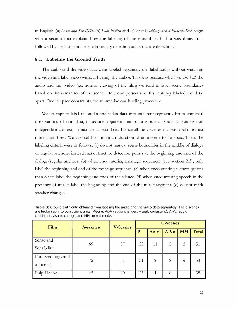
Table 3: Ground truth data obtained from labeling the audio and the video data separately. The c-scenes are broken up into constituent units: P-pure, Ac-V (audio changes, visuals consistent), A-Vc: audio consistent, visuals change, and MM: mixed mode.

C-Scenes Film A-scenes V-Scenes

P Ac-V A-Vc MM Total

Sense and

Sensibility 69 57 33 11 5 2 51

Four weddings and

a funeral 72 61 31 8 8 6 53

Pulp Fiction 45 40 25 4 8 1 38

23

Note, that an a-scene and v-scene are denoted to be synchronous if they less than 5 sec.

apart.

8.2. Scene Change Detector Results

There are several parameters that we need to set. The memory and attention span sizes

for the audio and video scene detection algorithm, and the synchronization parameter WC,

which we set to 5 sec (i.e. c-scene boundary is marked when the audio and video scenes are

within 5 sec. of each other). For detecting video coherence, video we set the attention span

to be 8 sec. (in accordance with our labeling rule) and the size of the memory is set to 24sec.

In general, increasing the memory size reduces false alarms, but increases misses.

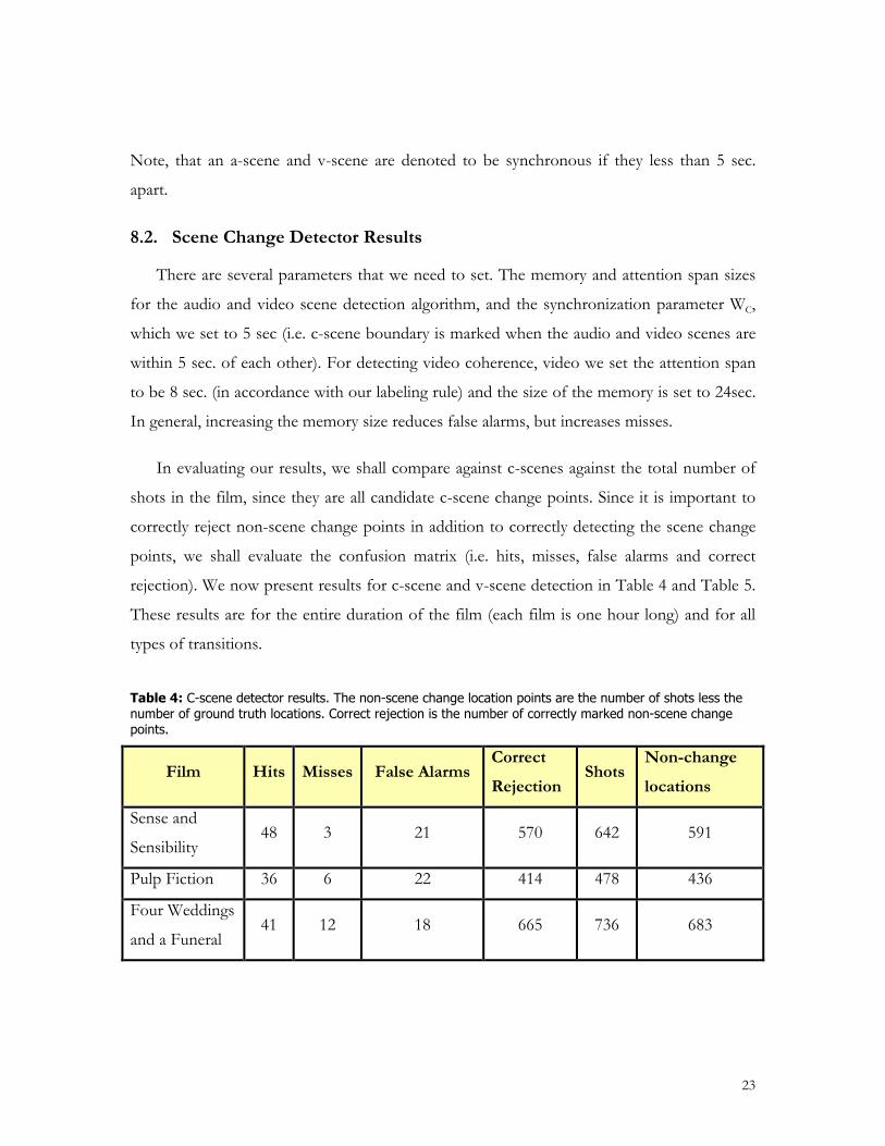
In evaluating our results, we shall compare against c-scenes against the total number of

shots in the film, since they are all candidate c-scene change points. Since it is important to

correctly reject non-scene change points in addition to correctly detecting the scene change

points, we shall evaluate the confusion matrix (i.e. hits, misses, false alarms and correct

rejection). We now present results for c-scene and v-scene detection in Table 4 and Table 5.

These results are for the entire duration of the film (each film is one hour long) and for all

types of transitions.

Table 4: C-scene detector results. The non-scene change location points are the number of shots less the number of ground truth locations. Correct rejection is the number of correctly marked non-scene change points.

Film Hits Misses False Alarms Correct Rejection

Shots Non-change locations

Sense and

Sensibility 48 3 21 570 642 591

Pulp Fiction 36 6 22 414 478 436

Four Weddings

and a Funeral 41 12 18 665 736 683

24

Table 5: V-scene detector results for the three films.

Film Hits Misses False Alarms Correct

Rejection Shots

Sense and

Sensibility 52 5 22 579 642

Pulp Fiction 38 2 20 458 478

Four Weddings

and a Funeral 49 12 41 695 736

The result shows that the c-scene and the v-scene detectors work well, with a best c-

scene detection performance of 94% detection for the film Sense and Sensibility, and a best

case v-scene detection performance of 95% in the case of Pulp Fiction. There are two sources

of error in our system: (a) uncertainty in the location of the audio labels due to human

uncertainty and (b) misses in the video shot boundary detection algorithm. Shot misses cause

the wrong key-frame to be present in the buffer, thus causing an error in the minima

location. In the film Four Weddings and a Funeral, there is a sequence of four c-scenes that is

missed due to very low chrominance difference between these scenes; it is likely that the

labeler managed to distinguish them on the basis of a semantic grouping of the shots. A

significant portion of the false alarms were cases that were correct from purely

computational standpoint, but wrong semantically. We discuss them in section 9.

We now briefly compare our results with prior work. In [5], the authors segment film

data on the basis of an adaptive shot clustering mechanism. They do not consider audio data

or the duration of the shot while segmenting the video. There is an important synergy

between audio and video that will not be examined in their work. Also, a semantically

meaningful scene can also be a few shots (or even a single shot), but of a long duration.

Hence, utilizing the duration of the shots, is important for segmentation. They also do not

consider the role of structure (especially dialogs) while grouping shots into a scene. Prior

work done in video scene segmentation used visual features alone [30], [7]. There, the

authors focus on detecting scene boundaries for sitcoms (and other TV shows) and do not

25

consider films. However, since we expect the v-scenes in sitcoms to be mostly long, and

coherent, we expect our combined audio visual detector to perform very well.

8.3. Structure Detection Results

In this section, we present our structure detection results. The statistical tests that are

central to the dialogue detection algorithm make it almost parameter free. These test are

used at the standard levels of significance (α = 0.05). The sliding window size Tw (6 frames).

The results of the dialog detector (Table 5) show that it performs very well. The best result is

a precision of 1.00 and recall of 0.91 for the film Sense and Sensibility. The misses are primarily

due to misses by the shot-detection algorithm. Missed key-frames will cause a periodic

sequence to appear less structured.

Table 6: The table shows the dialogue detector results for the three films. The columns are: Hits, Misses, False Alarms, Recall and Precision.

Film H M FA Recall Precision

Four Weddings and a Funeral 16 4 1 0.80 0.94

Pulp Fiction 11 2 2 0.84 0.84

Sense and Sensibility 28 3 0 0.91 1.00

There has been prior work [30][31] to determine dialogs in video sequences. The results

there are also good, however, they need to set cluster threshold parameters. In contrast, our

algorithm is almost parameter free.

9. Discussing C-Scene detector breakdowns

In this section we shall discuss three situations that arise in different film-making

situations. In each instance, the 180 degree rule is adhered to and yet our assumption of

chromatic consistency across shots is no longer valid.

1. Sudden change of scale: A sudden change of scale accompanied by a change in

audio cannot be accounted for in our algorithm. This can happen in the following

26

case: a long shot12 shows two people with low amplitude ambient sound; then, there

is a sudden close up of one person as he starts to speak. Detecting these breaks,

requires understanding the semantics of the scene. While labeling, these types of

scenes get overlooked by the labeler due to semantic grouping and hence are not

labeled as change points.

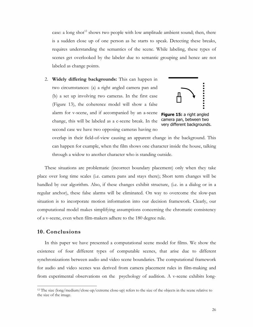
2. Widely differing backgrounds: This can happen in

two circumstances: (a) a right angled camera pan and

(b) a set up involving two cameras. In the first case

(Figure 13), the coherence model will show a false

alarm for v-scene, and if accompanied by an a-scene

change, this will be labeled as a c-scene break. In the

second case we have two opposing cameras having no

overlap in their field-of-view causing an apparent change in the background. This

can happen for example, when the film shows one character inside the house, talking

through a widow to another character who is standing outside.

These situations are problematic (incorrect boundary placement) only when they take

place over long time scales (i.e. camera pans and stays there); Short term changes will be

handled by our algorithm. Also, if these changes exhibit structure, (i.e. in a dialog or in a

regular anchor), these false alarms will be eliminated. On way to overcome the slow-pan

situation is to incorporate motion information into our decision framework. Clearly, our

computational model makes simplifying assumptions concerning the chromatic consistency

of a v-scene, even when film-makers adhere to the 180 degree rule.

10. Conclusions

In this paper we have presented a computational scene model for films. We show the

existence of four different types of computable scenes, that arise due to different

synchronizations between audio and video scene boundaries. The computational framework

for audio and video scenes was derived from camera placement rules in film-making and

from experimental observations on the psychology of audition. A v-scene exhibits long-

12 The size (long/medium/close-up/extreme close-up) refers to the size of the objects in the scene relative to the size of the image.

Figure 15: a right angled camera pan, between two very different backgrounds.

27

term consistency with regard to lighting conditions and chromaticity of the scene. The a-

scene shows long term consistency with respect to the ambient audio. We believe that the

computable scene formulation is the first step towards deciphering the semantics of a

semantic scene.

We showed how a causal, finite memory model formed the basis of our audio and video

scene segmentation algorithm. In order to determine audio scene segments we determine

correlations of the feature data in the attention span, with the rest of the memory. The

maxima of the rate of increase of the correlation is used to determine scene change points.

We use ideas of recall and coherence in our video segmentation algorithm. The algorithm

works by determining the coherence amongst the shot-lets in the memory. A local minima

criterion determines the scene change points.

We derived a periodic analysis transform based on the topological properties of the

dialog to determine the periodic structure within a scene. We showed how one can use the

Student�s t-test to detect the presence of statistically significant dialogues. We also showed

how to determine silences in audio.

We derived semantic constraints on the computable scene model, and showed how to

use the silence and structure information along with audio and video scene boundaries to

resolve certain ambiguities. These ambiguities cannot be determined with using just the a-

scene and the v-scene detection models.

The scene segmentation algorithms were tested on a difficult test data set: three hours

from commercial films. They work well, giving a best c-scene detection result of 94%. The

structure detection algorithm was tested on the same data set giving excellent results: 91%

recall and 100% precision. We believe that the results are very good when we keep the

following considerations in mind: (a) the data set is complex and (b) the shot cut detection

algorithm had misses that introduced additional error.

There are several clear improvements possible to this work (a) the computational model

for the detecting the video scene boundaries is limited, and needs to tightened in view of the

model breakdowns discussed. One possible improvement is to do motion analysis on the

video and prevent video scene breaks under smooth camera motion. (b) The v-scene

28

detection algorithm should dynamically adapt to the low-contrast scenarios to improve

performance. (c) Since shots misses can cause errors, we are also looking into using entropy-

based irregular sampling of the video data in addition to the key-frames extracted from our

shot-segmentation algorithm. Current work includes generating video skims using these

computable scenes [25].

11. Acknowledgement

The authors would like to thank Di Zhong for help with the shot boundary detection

algorithm.

12. References

[1] A.S. Bregman Auditory Scene Analysis: The Perceptual Organization of Sound, MIT Press,

1990.

[2] D.P.W. Ellis Prediction-Driven Computational Auditory Scene Analysis, Ph.D. thesis, Dept. of

EECS, MIT, 1996.

[3] Bob Foss Filmmaking: Narrative and Structural techniques Silman James Press LA, 1992.

[4] B. Grosz J. Hirshberg Some Intonational Characteristics of Discourse Structure, Proc. Int.

Conf. on Spoken Lang. Processing, pp. 429-432, 1992.

[5] A. Hanjalic, R.L. Lagendijk, J. Biemond Automated high-level movie segmentation for advanced

video-retrieval systems, IEEE Trans. on CSVT, Vol. 9 No. 4, pp. 580-88, Jun. 1999.

[6] J. Huang; Z. Liu; Y. Wang, Integration of Audio and Visual Information for Content-Based

Video Segmentation, Proc. ICIP 98. pp. 526-30, Chicago IL. Oct. 1998.

[7] J.R. Kender B.L. Yeo, Video Scene Segmentation Via Continuous Video Coherence, CVPR '98,

Santa Barbara CA, Jun. 1998.

[8] R. Lienhart et. al. Automatic Movie Abstracting, Technical Report TR-97-003, Praktische

Informatik IV, University of Mannheim, Jul. 1997.

[9] J. Meng S.F. Chang, CVEPS: A Compressed Video Editing and Parsing System, Proc. ACM

Multimedia 1996, Boston, MA, Nov. 1996

29

[10] J. Nam, A.H. Tewfik Combined audio and visual streams analysis for video sequence segmentation,

Proc. ICASSP 97, pp. 2665 �2668, Munich, Germany, Apr. 1997.

[11] R. Patterson et. al. Complex Sounds and Auditory Images, in Auditory Physiology and Perception

eds. Y Cazals et. al. pp. 429-46, Oxford, 1992.

[12] S. Pfeiffer et. al. Abstracting Digital Movies Automatically, J. of Visual Communication and

Image Representation, pp. 345-53, vol. 7, No. 4, Dec. 1996.

[13] W.H. Press et. al Numerical recipes in C, 2nd ed. Cambridge University Press, 1992.

[14] L. R. Rabiner B.H. Huang Fundamentals of Speech Recognition, Prentice-Hall 1993.

[15] K. Reisz, G. Millar, The Technique of Film Editing, 2nd ed. 1968, Focal Press.

[16] C. Saraceno, R. Leonardi Identification of story units in audio-visual sequences by joint audio and

video processing, Proc. ICIP 98. pp. 363-67, Chicago IL. Oct. 1998.

[17] Eric Scheirer Malcom Slaney Construction and Evaluation of a Robust Multifeature

Speech/Music Discriminator Proc. ICASSP ′97, Munich, Germany Apr. 1997.

[18] S. Pfeiffer et. al. Automatic Audio Content Analysis, Proc. ACM Multimedia ′96, pp. 21-30.

Boston, MA, Nov. 1996,

[19] John Saunders Real Time Discrimination of Broadcast Speech/Music, Proc. ICASSP ′96, pp.

993-6, Atlanata GA May 1996.

[20] S. Sharff The Elements of Cinema: Towards a Theory of Cinesthetic Impact, 1982, Columbia

University Press.

[21] L.J. Stifelman The Audio Notebook: Pen and Paper Interaction with Structured Speech, PhD

Thesis, Program in Media Arts and Sciences, School of Architecture and Planning,

MIT, Sep. 1997.

[22] S. Subramaniam et. al. Towards Robust Features for Classifying Audio in the CueVideo System,

Proc. ACM Multimedia ′99, pp. 393-400, Orlando FL, Nov. 1999.

[23] H. Sundaram S.F. Chang Audio Scene Segmentation Using Multiple Features, Models And Time

Scales, ICASSP 2000, International Conference in Acoustics, Speech and Signal

Processing, Istanbul Turkey, Jun. 2000.

30

[24] H. Sundaram, S.F. Chang Determining Computable Scenes in Films and their Structures using

Audio-Visual Memory Models, Proc. Of ACM Multimedia 2000, pp. 95-104, Nov. 2000,

Los Angeles, CA.

[25] H. Sundaram, S.F. Chang, Codensing Computable Scenes using Visual Complexity and Film

Syntax Analysis, submitted to Proc. ICME 2001.

[26] H. Sundaram, S.F Chang Computable audio scene boundary detection using a listener memory

model, ADVENT Tech. Report, Dept. of Electrical Engg., Columbia University, Jan.

2001.

[27] H. Sundaram, S.F Chang Topological analysis of Video Sequences, ADVENT Tech. Report,

Dept. of Electrical Engg., Columbia University, Mar. 2001.

[28] S. Uchihashi et. al. Video Manga: Generating Semantically Meaningful Video Summaries Proc.

ACM Multimedia ′99, pp. 383-92, Orlando FL, Nov. 1999.

[29] T. Verma A Perceptually Based Audio Signal Model with application to Scalable Audio

Compression, PhD thesis, Dept. Of Electrical Eng. Stanford University, Oct. 1999.

[30] M. Yeung B.L. Yeo Time-Constrained Clustering for Segmentation of Video into Story Units,

Proc. Int. Conf. on Pattern Recognition, ICPR ′96, Vol. C pp. 375-380, Vienna Austria,

Aug. 1996.

[31] M. Yeung B.L. Yeo Video Content Characterization and Compaction for Digital Library

Applications, Proc. SPIE �97, Storage and Retrieval of Image and Video Databases V,

San Jose CA, Feb. 1997.

[32] T. Zhang C.C Jay Kuo Heuristic Approach for Generic Audio Segmentation and Annotation,

Proc. ACM Multimedia ′99, pp. 67-76, Orlando FL, Nov. 1999.