—

-+

s

t-do,

plex

Sensor and Simulation Notes

Note 201

September 1974

Modes on a Finite-Width, Parallel-Plate SimulatorI. Narrow l?lates

Lennart.NarinDikewood Corporation, Westwood Research Branch

Los Angeles, California

Abstract

The higher-order TE and TM nodes on a simulator consisting of

parallel, narrow plates are studied. Expressions for the com-

transverse propagation constants are found showing that the

TM modes are less damped as they propagate along the line than are

the TE modes. The transverse variation of both the longitudinal

and the transverse field components of the lowost TM modes are

mapped. A general integral equation is also derived which 1s suit-”

able for the numerical evaluation of the leaky modes on a parallel-

plate simulator having an arbitrary separation-to-width ratio of the

parallel plates.

t

Contents

Abstract

Introduction

Integral Equations for the Field

Solution of the IntegraIEquation

Case of Narrow Plates

IV Modes on Narrow Plates

in the

v Fredholm Integral Equation of the Second “Kind

for the TM and TE Fields

Appendix A

Appendix B

Acknowledgement

References

Page

“1

5

9

14

20

52

58

67

69

70

● “S

2

* b

●

9

Figure

1

2

3

4a

4b

4C

5a

5b

5C

6

7a

7b

8a

Illustrations

Schematic picture of ATLAS I and 11 simulators.

Two, finite-width, parallel plates.

Transverse propagation constant of TM modes.

The variation along the y-axis of the absolute value of thenormalized electric field for the TEM mode (n = O) and thelowest antisymmetric TMmodes (n = 1,2,3), The plates arelocated at y/h = *1.

The variation along the y-axis of the real part of thenormalized electric field for the TEM mode (n = O) and thelowest antisynunetricTMmodes (n = 1,2,3), The plates arelocated at y/h = il.

The variation along the y-axis of the imaginary part of thenormalized electric field for the TEM mode (n = O) and thelowest antisymmetric TMmodes (n = 1,2,3). The plates arelocated at y/h = fl,

The variation along the x-axis of the absolute value of thenormalized electric field for the TEM mode (n = O) and thelowest antisymmetric TMmodes (n = 1,2$3). The plates arelocated at ylh = *1.

The variation along the x-axis of the real part of thenormalized electric field for the TEY mode (n = 0) and thelowest antisymmetric TMmodes (n = 1,2,3). The plates arelocated at y/h = tl.

The variation along the x-axis of the imaginary part of thenormalized electric field for the TEM mode (n = O) and thelowest antisymmetric TMmodes (n = 1,2,3). The plates arelocated at y/h = il.

The electric field lines (solid lines) and the magneticfield lines (broken lines) of the TEM mode.

The electric field lines (solid lines) and the magneticfield lines (broken lines) of the real part of the firstantisymmztric TM mode.

The electric field lines (solid lines) and the magneticfield lines (broken lines) of the imaginary part of thefirst antispmetric THmode,

The electric field lines (solid lines) and the magneticfield lines (broken lines) of the real part of the secondantisymwtric TX mode.

3

.—=.

Page

6

10

23

28

29

30

32

33

34

35

36

37

PageFigure

8b

9

10a

10b

Ioc

10d

10e

lof

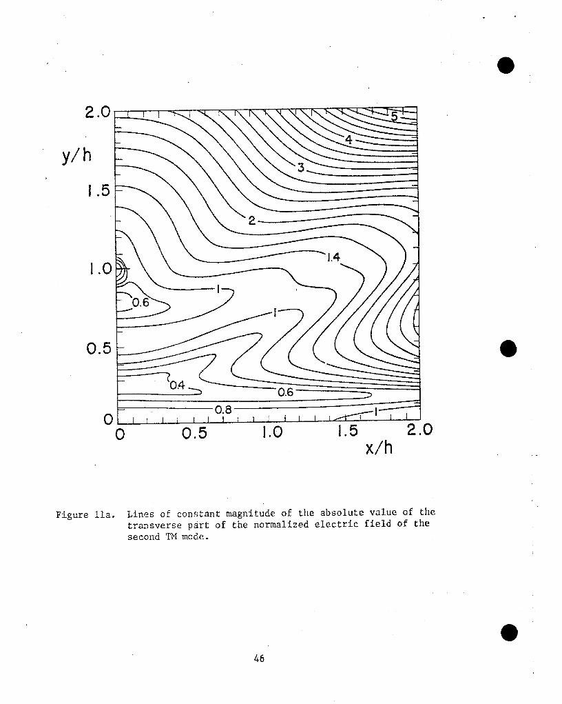
lla

Ilb

lIC

Ild

He

The electric field lines (solid lines) and the magnetic fieldlines (broken lines) of the imaginary part of the secondantisymmetri.cTM mode.

Lines of constant-magnitudeof the normalized electric andmagnetic fields of the TEM mode.

Lines of constant magnitude o~the absolute value of thetransverse part of the normalized electric and magnetic fieldsof the first TM mode.

Lines of constane Magnitude of the real part of the transversepart of the normalized electric and magnetic fields of thefirst TM mode.

Lines of constant magnitude of the imaginary pare of thetransverse part of the normalized electric and magnetic fieldsof the first TM mode.

Lines of constant magnitude of the absolute value of thelongitudinal part of the normalized electric field of thefirst TM mode.

Lines of constant magnitude of the real part of thelongitudinal part of the normalized electric field of the firstTM mode.

Lines of constant magnitude of the imaginary part of thelongitudinal part of the normalized electric field of thefirst TM mode.

Lines of constant magnitude of thetransverse part of the normalizedof the second TM mode.

Lines of constant magnitude of the

absolu~e value of theelectric and magnetic fields

real part of the transversepart of the normalized electric and magnetic fields of thesecond TM mode.

Lines of constant magnftude of the imaginary part of thetransverse part of the normalized electric and magnetic fieldsof the second TM mode.

Lines of constantlongitudinal partsecond TM mode.

Lines of constantlongitudinal partsecond TM mode.

Lines of constantlongitudinal partsecond TM mode.

The surfaces S,

magnitude–of the absolute value of theof the normalized electric

magnitude of the real partof the normalized electric

magnitude of the imaginaryof the normalized electric

field of the

of thefield of the

part of ehefield of the

~; So and the boundary curve L.

4

38

39

40

41

42

43

44

45

46

47

48

49

50

5159

—

I, Introduction

● Many EMP simulators, such as the ATIAS I and 11, the ARES and the

ALECS, make use of a parallel-plate transmission line as a guiding structure

for the electromagnetic field (see Fig. 1). One reason for using parailel-plate

simulators is that they support a TEM mode. In many of these simulators the

field distribution of the TEMmode is nearly uniform over a significant portion

of their cross section. For this reason and the reason that the TEMmode

propagates with the speed of light, the TEM mode provides a good approximation

to the free-space nuclear EME’. The TEMmode propagates at all frequencies but

for frequencies such that the free-space wavelength is of the same order as

the cross-sectional dimensions of the simulator the TEMmode alone may not be

the dominant part ‘ofthe simulator field. In most cases it is desirable to

launch fast rising pulses on the parallel-plate simulators whose risetimes are

significantly smaller than the transit time across the simulator. In doing

so the simulator field will consist not only of the TEM mode but.also of higher

order modes and a continuous spectrum.

The properties of the TEMmode on two parallel plates have been investigated[1-6]

using conformal mapping techniques o The effect of replacing the parallel

e[1,7]

plates by a number of parallel wires has also been investigated . The..----.._.=,,..=,,

transient curren~s’o;a simulator consisting of two parallel wires where each

wire is fed

in [8], It

manner, the

sum plus an

by a slice-generator with a step-function voltage has been studied .

is found in.[8] that when the two wires are fed in a push-pull

transient induced current can be expressed in terms of an infinite

infinite integral. One term in the sum represents the contribution

from the TEMmode$ whereas the other terms can be interpreted as the contribution

from higher order modes, the properties of which will be discussed below, The

combined contribution from all modes represent the contribution from the discrete

part of the spectrum, whereas the integral represents the contr~bution from tlio

continuous part of the spectrum.

The discrete spectrum of an open waveguide has properties which are

different from those of the discrete spectrum of a closed waveguide, In regions

of finite extent bounded by impenetrable walls, i.e., closed regions, the modes

(which are the source-free solutions of the Maxwell equations) generally posseus

orthogonality and completeness properties such that an arbitrary field distribution

5

—

TER MI NATION ●

TERMINATION

PULSER

I

Figure 1. Schematic picture of ATLAS I arid11 sirnulELtOrfi..,

6

.

● can be represented by their superposition. These modes are square integrable

over the cross section of the waveguide (because they have finite energy),

satisfy the source-free Maxwell equations and the appropriate boundary conditions

on the walls of the waveguide. In regions of infinite extent, i.e., open regions,

there may exist a corresponding discrete spectrum. However, to get a complete

representation of the field these modes must in general be supplemented by a

continuous spectrum. All modes of the discrete spectrum satisfy the source-free

field equations and the boundary conditions on the surface of the waveguide. In

contradistinction to the modes on a closed waveguide many modes of the discrete

spectrum of an open waveguide are not–square integrable on the cross section of

the waveguide. In fact, the field components of these modes OL’more aptly Lhe

leaky modes grow exponentially in the transverse direction far away from the

waveguide. Mathematically, this fact can be stated as follows: the propagation

constants of the leaky modes belong to the Riemann sheet in which the radiation

condition is violated. Although these modes in general do not form a complete

set of orthogonal functions, they can nevertheless be employed to obtain

econvergent representations of the field in certain regions in space, for example,

the region between the two parallel plates in a parallel-plate simulator.

Some comments are now in order concerning a method that may be used when

determining the excitation coefficient of each leaky mode. The “ordinary”

technique of matching fields at a cross section of a waveguide, which is so

useful when determining the excitation coefficient of each mode in a closed

waveguide, does not necessarily apply to open waveguides, since the leaky modes

are neither square integrable nor do they form a complete set of functions,

Instead of matching fields at a cross section of a waveguide the excitation

coefficients of the leaky modes can be obtained by requiring that the total

field satisfies the boundary conditions on the waveguide walls (cf. [8]).

Finally, we mention that-”the-leakymodes are the nontrivial solutions of

the Maxwell equations in.two dimensional regions which are exterior to a region

of finite–extent. Therefore, the leaky modes in two dimensions are the counter-

parts to the natural modes[9] in three dimensions.

This note is a continuation of a previous note[8]

which treats the transient

field around two parallel P?iresexcited at a delta gap. Whereas the attention

@ was focused on the time history of the induced currents on the wires in ~8].

7

.

this note places more emphasis on the field distribution of certain leaky modes

on two narrow parallel plates. These modes are found by formulating two @

different scalar integral equations of the first kind for the longitudinal

components of the electric and magnetic fields, respectively. When the

separation between the plates is large compared to their width these integral

equations can be solved analytically by first transforming them into a Fredholm

integral equation of the second kind which in turn can be solved using perturba-

tion techniques. The results of the field calculations are presented in graphical

forms for the transverse components of the”electric and magnetic fields of the

two lowest TM modes. Graphical results are given of the magnitude of the electric

field of the three lowest TM modes and of the transverse propagation constant.

A general method of reducing scalar scattering from open surfaces to the

solution of Fredholm integral equations of the second kind is given in the

Appendix. Both the Dirichlet problem and the..Neumannproblem are discussed.

These integral equations are then used to derive suitable integral e~uations of

the second kind for the TE fields and the TM fields on two parallel plates of

finite width. Certain properties of the integral equations are derived. It iS

also shown how they can be used to numerically determine the transverse, complex ●propagation constant and field distribution of the leaky modes on two parallel

plates of arbitrary separation-to-widthratio. Due to—

numerical calculations they are left to a future note.

the complexity of these

—.

II. Integral Equations for the Field

Consider a waveguide that consists of two parallel plates of finite width,

the width of each plate being 2W and the distance separating the two plates

being 2h, (see Fig. 2), The waveguide is excited by an incident electro-

‘nc(r,t), 3&c(~, t). To find the scattered field C(r,t),magnetic field ~ _ _ --

3C(r,ti)Laplace transform methods will be used,——

and similarly

the z-axis is

axes span the

Fig. 2). The

Wm

g(x,y,c,s) = H C(r,t)exp(-zz)exp(-st)dzdt (1)---m -m

for the magnetic field. The coordinate system is so chosen that

directed along the axis of the waveguide and that the x and y

plane which is perpendicular to the axis of the waveguide (see

transverse field components in the-Laplace transform domain are

related to the longitudinal components in that domain via

@

gt(x,y,c,s) = -Cp-2VtEz(x,y,L,s) - spop-*ixvtHz(x,Y& ys)

(2)

IIt(x,y,c,s)= -Lp-%tllz(x,y,c,s) + Seop‘2;xVtEz(x,y,G~s)

where p = m, c is the vacuum speed of light and the index t

denotes the transverse field components, Thus, once the longitudinal components

of-both the electric and magnetic fields are deter-minedin the Laplace trans-

form domain, the scattered field &(r,t) is given by (2) and the inverse-—

Laplace transform integral

1C(r,t) =—

)[J

12ni ~ X 1~(x,y,~,s)exp(~z)d; exp(st)ds——

s cc

where C and Cs c

are paths of integration parallel to the imaginary axes

the complex s and G planes. The scattered magnetic field 3C(r,t) is--

determined using a similar procedure.

o From the-Maxwell equations it follows that both Ez and Hz satisfy

the two-dimensional Helmholtz equation,

(3)

9

,

2hw

‘+--2W

Figure 2. Two$ finf.te-wfdth$paralIel plates.

. ,

V;EZ - p2Ez = 0, V$Z - p2Hz = O (/+)

and the boundary conditions on the plates imply that

Ez + E:nc_=o~ on‘+

and S

aH 2~Einc.

~+~Einc-~~=ay SPO ax

o on s+ and Sx

o

(5)

where S+ (S-) denotes the cross-section of the upper (lower) plate, i.e.,

in mathematical terms Sk = {x,Y:IxI<w, y = ih}, One observes tha~ Ez (lIZ)

is given by the solution of a Dirichlet (Neumann) boundary-value problem.

Next.,integral equations will be formulated the solutions of which enable “

one to determine E and H Therefore, first note that Ez andz z“

(a/ay)Hz

are continuous everfihere (including on St). However, (a/ay)Ez and Hz can

obe discontinuous across S+ and so the following quantities are introduced

[

aE 2Ef+(x) = lim e (x,th+ C,~,S)

~+() ay 1-#(x,fh- c,~,s)

(6)

(sHo)-lgJx) = lim [Hz(x,th + ~,~,s) - iz(x,~h - e,c,s)] .@o

The paths of integration in (3) has to be chosen so that the scattered field

satisfies the radiation condition at infinity. This implies that Ez and Hz

satisfy the radiation condition as (X2 +Yzp tends to infinity. Keeping

this in mind the Green’s theorem gives

fwEz(x,y,~,s) =

JG(x,y,x’,h;p)f+(x’)dx’+

JG(x,y,x’,-h;p)f-(x’)dx’

-w -w

(7)

~

w aG“w

SUoHz(x,y,L,s) = --w ~

(x,y,x’,h;p)g+\x’)dx’-~

~ (x,y,x’,-h;p)g-(x’)dx’-v ay

o where

G(x,y,x’,y’;p) = *.o(pmy - ,,)2)

11

and KO(E) is the modified Bessel function of the first kind. !llaking.the

y-derivative ~f the latter of the equations in (6) and using the fact that the

Green’s function satisfies the differential equation

V:G - P2G = O, x+x’ and y + yt (8)

one gets the following expression

aH

( )[~2 w

Spo& (x,y,&(s) = --- p2 G(x,y,x’,h;p)g+(x’)dx’ax2 “w

Iw

+ ---1G(x,y,x’,-h;p)g-(x’)dx’. (9)-w —

By requiring that the total longitudinal electric field vanishes on the

plates one obtains the following set of integral equations for f+(x) ‘

~

w

f

w

G(&h#J;p)f+(x’)dx’ -t- G(~h,x~,-h;p)f~(x’)dx’= a+(x), 1X1 <w-w -w

Iw

~

wG(x,-h,x’,fip)f+(x’)dx’-f- G(x,-h,x’rh;p)f-(x’)@’=a-(x), [xl ~ w

-w -w

where

a+(x) = -E~(x,lh,g,s).

(10)

Similarlj, the boundary conditions (5) for (~/ay)Hz on the plates result in

the following differential-integralequations for g+(x)

(~- ~)[~~(x,hx*;P~~+{x)dx, ~-~:~,h~rh~p)g~x)dxj = 13+(x],

1X1 < w

12

.

“owhere

This set of differential integral equations can be integrated to yield the

following set of i;tegral equations

1wG@h#,h; p)g4(x’)dx’ + r G&,h&’r~p )g_(x’)dx’

J -w J -w—

~

w= A+ cosh(px) +-B+ stnh(px) +

-w

sinh(plx-x’1) ~ ~x,)dx,2p +

(12)

Iw

\

w

G6t,-h#,h;p)g+(x’)dx’ + G(x,-h,x’,-h;pjg-(x’)dx?-w -w

= A_ cosh(px) +“B- sinh(px)+\

w sinh(plx-x’1) ~ ~xf)dx,2p

-w

where A. and B. are constants of integration to be determined~ ~

conditions which require that

2+g+(x) - (W2 - x ) as X+kwo

from the edge

The integral equations (10) and (12) constitute the mathematical formulation

of the scattering problem. In the next section the two sets of integral equations

(10) and (12) will be solved for narrow plates, i.e., when w << h.

,’

13

111. Solution of the Integral Equations in the Case of Narrow Plates

When the width of%he-p-lates is small compared to the distance separating

the two places an approximate solution of the sets of integral equations (10)

and (12) can be found using analytical techniques. In the first part of this

section a solution of (10) will be obtained from

the TM field (E waves) can be determined. Then,

TE field (H waves).

A. The Transverse Magnetic Field

which aU the properties of

(12) wiU be solved for the

The set of two coupled integral equations (10) can be transformed into

two uncoupled integral equations in the following way: first introduce the

two functions Uf(x) = f+(x) t f-(x), so tha~ 2ft(x) = u+(x) t u (x) and

then substitute them into (10). By adding and subtracting the two equations

in (10) one arrives at the following two uncoupled integral equations

\

w

~

wG(x,h,x’,h;p)uJx’)dx’ t G(x,h,x’,-h;p)ut(x’)dx’= U+(X)

-w “w(13)

where P+(x) = U<K(x)t a (x). The solution u+ corresponds to the case where

the longitudinal current on one plate has the same magnitude and direction as

that on the other plate, whereas the solution u corresponds to the case

where the longitudinal current on one plate has the same magnitude but opposite

direction as that on the other plate. The terms “push-push” and “push-pull”

were used in [8] for these two cases.

Now, consider the case where w <~ h. In this case there exists a

complex p SLIChthat lPw\ ‘< ~ but Iphl is not necessarily small. With

this restriction on p one can approximate Che kernels in (13) by the following

expressions

G(x,h,x’,h;p)= (2m)-1{-y - ln(plx-x’l/2) +p2(x-x’)2/4[1 - y - ‘~n(p[x-xf~/2)J}

[14)

G(x,h,x’,-h;p)w (2#[Ko(2ph) - (X-X’)2p/(2h)Kl(~ph)]

..’1

“o14

.

where y is Euler’s constant, Y sz0.5772..... Using these approx~ate

expressions for the kernels in (13) one arrives at the following approximate

integral equations for u+,

r ~wIn(plx-x’l)u+(x’)dx’ - [ln 2- y t Ko(2ph)]u+(x’)dx’-w -w

~

w-t L+(x,x’)u+(x’)dx’ = -21TP+(X)

-w -

(15)

where

L+(x,x’) = p2(x-x’)2[ln(plx-x’1) - In 2+y f (2/ph)K1(2ph)]/4.

}

The integral equation (15) where the kernel has a logarithmic singularity at

x=x’ can be transformed into the following l?redholmintegral equation of

the second kind with the aid of the Cauchy inEegral[10]

@ln(2/pw)-ytKo(2ph) w

Ut(x) +I

u+(x’)dx’

P ‘w-rln2 w-x

w w L+(x’,x’’)u+(x”)

‘f-~1-

dx~dx’f

IT2ln2 W2-X2 ‘w ‘w C2

-t-w \‘~dw

[J— — 1L+(x’,x’’)u+(x’’)dx”dx’

2/w~ -wXf-x dx‘

lT-w -

r.-i n

1w llt(x’)

\

w p;(x’){wz-x”

=

ITi;wfi‘w m ‘x’ - .k?‘w - “-xdx‘ (16)

whereI

denotes the principal-value integral.

The

following

● small, so

of (16) is small compared to the contribution from the first two terms. ‘l’lluBJ

integral equation (16) can be solved iteratively by making the

observation: when \pwl <.1 the norm of the kernel Ly(x,x’) fR

that the contribution from the last two terms on the I.eft-ilandside

15

to the first approximation one

equation

has u+ = u; where u: satisfies the integral

Iw p+(x’)

/

mw p:(x’) w -x= -—m’1.22‘w ti ‘“ 2+? ‘w - “-x

dx’.

.;

A closed-form solution of Lhis integral equation is found to be

,F-2-X2 XT-X

To find a better approximation for Ut one writes

dxt.

‘+U:u+ = u+

where Ilu;ll‘< Ilu;ll* Substituting the expression (19) into (16) and taking

into account the facts that the norm of L+(x,x’) is small and that u:

satisfies (17) the following expression for u: is obtained,

1w w Ly(x’,x’’)u~(x”)

u:(x) =w

lj-dx‘dx”

N2[ln(4/pw)-ytKo(2ph)]~~- ‘W ‘W ~~i

w ‘~riwI X’-x [/&T

1

L+(x’,x’’)u~(x’’)dx”dX’.2Jwq” -w -w -?T

(19)

(20)

The analytical properties in the complex p-plane of the solutidna (18)

and (20) will now be investi~ated, When the incident field is a holoamrpkfc

function of p iL follows immediately from (20) that u+ has two types of-..

singularities: a branch-point at p=cl and poles at those values of p for

16

.

.0 which the homogeneous integral equation (16) has a nontrivial solution. Each

one of these poles corresponds to a mode and in the next section certain

properties of these modes will be investigated. It should also be pointed

out that although these analytical properties in the p-plane of the scattered

field has only been proven for narrow plates, they are shared by the scattered

field on a parallel plate waveguide of arbitrary width-to-separation ratio.

B. The Transverse Electric Field

The transverse electric field is determined from the solution of the

set of integral equations (12). Similarly to the T’Mcase one introduces the

functions v+(x) = g+(x) * g_(x), so that 2gt(x) = v+(x) * v-(x) and

Vt(x) satisfies the integral equation

I

w

\

wG(x,h,x’,h;p)v~(x’)dx’ f G(x,h,x’,-h;p)v+(x’)dx’

-w -w

= Ct cosh(px) i-Dt sinh(px) -f-Vt(x) (21)

where - wv+(x) = J (2p)-1sinh(plx-x’\)[6+(x’) t B-(x’)]dx’

-w

.C+ =A+ ~A-, D+ =B+~B

and the constants C+ and D& are determined from the edge conditions at

x = tw. By comparin~ (16) and (21) it-follows from (13), (18), (19), (20)

that one has the following approximate solution of (21),

VJX) = v:(x) + v;(x) (22)

where

2W

~-

w C+ cosh(px’)+ D+sinh(px’) + Vt(x’)v:(x) =

n[ln(4/pw)-ytKo(2ph)]& e

dx‘-w 2 ,2

-xi

2W

\

w [PC+ sinh(px’)+pD+ P’cosh(px’)+v;(x’)j W ‘X.. ——

r

dx‘X1-X (23)

~ JXZ -w

17 “

.

v:(x) =w

wz~ln(4/pw)-ytKa(2ph)]

w “Y(z7/=2]W- -w

Xt-x

rr1L+(xT,X’t)V~(X”)

&22

‘w-w - ti “’’x” ‘ o

[Jd“1

L (xf,x’’)v;(v’’)dx”dx’.=-J

.

(24)

To determine the unknown constants Ct and D+ one invokes the edge conditions-2 &at x = iw which require thaC v+(x) N (W2 - x ) as x + &, These

conditions result in the following equations

1ln(4/pw)-ytKQ(2ph)

=-/w[pc+

-w -

Iw C+ cosh(px’)+ D+sinh(px’)+vt(x’)

‘X’-w e

,2

.

<

Ei+xtsinh(px’) + pD+ cosh(px’) i-v~(x~)]

z ‘x’

f“= J [pc~ sinh(px’) +pD+cosh(px’) +V;(X’)]

r~ ‘X’ (25) O

-w -

from which one gets—

-1W u;(x~)+Fi(p,w,h)x’v;(x~)

c+ =\-

dx‘m[Io(pw)+pwIl(pw)F~(p,w,h)] -w

m

(26)

-1 r’av~(x’)D+ = -’xl

mpaIo(pa) J‘w m

where %

l?~(p,w,h)= ln(4/pw) - y tKo(2ph)

and In(c) is the modified Bessel function of the first kind.

‘,.

●18

,

● Again, it is noted that v+(x) has a branch point at the origin of the

p-plane besides poles for certain values of p. In the next section it will

be shown that there are no poles, however, for Ipwl << 1.

.–

●

19

Iv. Modes on Narrow Pletes

In the previous section it was pointed out that the scattered Eield has

two types of singularities in the complex p-plane, namely, a branch point at

P = O and poles. When evaluating the inverse Laplace transform integral (3)

the branch point shows up in the form of an integral around the corresponding

branch cut and the poles give rise to modes propagating along the waveguide[81,2 -2The z-dependence of these modes is given by exp[-z(s c

2+- Pn) ] where pn

has the value such that the homogeneous equations (10) or (12) have a non-

trivial solution. The quantity pn may be called the transverse propagation

constant of the mode and is equal to the imaginary un”it~iqes the transverse—.

wavenumber. To each mode one associates a f-ielddistribution.’ Later in this

section the transverse electric and magnetic fields of certain important _!fM

modes will be investigated. First, the transverse propagation constants for

both TM and TE modes will be obtained.

A. Transverse Propagation Constants of TMModes

The transverse propagation constants of the TM modes are given by the

poles in u+(x), i.e., by those values of p for which the homogene~us integral

equation (13) has a nontrivial solution. Using the perturbation methad employed

in Sec.11’ian approximate value of p is given by the nontrivial solution of

ln(2/pw)-y*Ko(2ph) wa;(x) -1-

~;:(x~)dx’ = O

n ln2 ~ ‘w -

which, after integration, yields

Jw

[1-n(4/pwl- Y ~ Ko(2ph)] ;;(x)dx = O.-w -

..(27) ,_

From (27) one notes that &~(x) is an even function of the form

~i;(x)= A/(w2 - X2)-%. Thu:, from (27) and (28) it is clear that. A;O

only when

ln(4/pw) - y ~ Ko(2ph) = O.

The determinental equation (29) for TM modes on cwo parallel, narrotiplates

20

(29)

—

—

,.

● can be compared with ”thatfor two parallel wires with radii a and separated

by a distance 2h. In the wire case the determinental equation is[8],

ln(2/pa) - Y ~ Ko(2ph) = O

and the factor of 2 difference in the logarithmic term between the

expressions can be accounted fo’rby noting that’the effective radius

strip is w/2, i.e., a strip of width 2W has the same capacitance

length as a cylinder with radius w/2.

The transcendental equation (29) has to be solved numerically,

(30)

two

of the

per unit ‘

and its

solutions are denoted by pin. The corresponding nontrivial solution of ~~

is then

(31)

o and ~~(x) is normalized so that

~

w~~(x)dx = 1, (32)

-w -

Note that this function is independent of p~n.

To get a more accurate value of the poles of U2(X) in (16) one

substitutes the expansions

into the homogeneous equation (16) and obtains the following equatfon

\

k +2whp~np:nKl(2p~nh)“ .1 >wpln-0:(’) - u+(x’)dx’ =

&

- At(x) (34)2-X2 -w -

Pp~nr ln2 w -x

●

,,21

where

A+(X) = ‘“)’--Tr31U2 W2-X2

+W r’

w

~r

L+(x’,X”)

-w -w +(wu2) (wZ-x”Z)

,.

dx‘dx”

[1

~dw L+(x’,x”)

—.z J-w X’-X

3&~dx‘

m 1‘w‘mdx’’dx’”— ., –—

.

By integrating (34) and using the fact that u:(x) is an even function not

identically equal-to zero the following expression for pin iS derived%

~ (P:n)3w2{T2+2-1.51T2In 2-(n2-8)y/4+(T2-8)[M&/2)t2(~P:n)-lKl (2hP:n)]/4}

P~n =.

@t2hp:nK1(2hp:n)]fa’zl

Equation (29) was solved numerically for the twelve lowest roots. These

values were then used to numerically evaluate P;n from (35). The results

of th~se calculations are shown in Fig. 3 and Table 1 where the normalized

quantity p~w = (pan + p~n)w is presented.

.:B. Transverse Propagation Constants of TE Modes

The transverse propagation constant for the TE modes are given by those

values of p for which the homogeneous integral equation (21) has a nontrivial

solution. Since the main concern of this note is the case where ~pwl c< 1 one

can, in the first approximation, neglect the second term on the left-hand side

of (23) and also makes the approximations cosh(px) R 1, sinh(px) * pX.

Thus, one has the following approximate homogeneous integral cqu~~~~n

ln(2/pW)-yfKfi(2Ph)

Iwv~(x’)dx’

-w -

2WC+ 2wpDTxz

MF7+E*

(36)

22

. .

●

.,

1

I I I I Iw/2.h =0.001 , 0.01

%

●

☎

●

☎

☛

☎

●

x●

x

●

x●

x●

x●

x*

%

●

☎

●

☎

●

x●

x●

%●

x●

x9

x●

xe

x x● ●

w/2h =0.

●

x

Ix x, x

I I-3 -2 -1

Figure

Re {2ph\

3. Transverse propagation constant of-TM mo~es.

2ph}

23

W/2h n Re{2P31 Irn{2p>} Re{2p~h} Im{2p;h}

0.01 1 -1.902 2.552 -2.084 !5.8362 -2.185 9.051 -2.252 12.2463 -2.303 15.430 -2.342 18.6114 -2.374 21.785 -2.400 24.9625 -2.423 28.128 -2.443 31.3056 -2.461 34,464 -2.478 37.6467 -2.493 40.797 -2.506 43.9598 -2.519 47.126 -2.532 50.3239 -2.543 53.454 -2.555 56.66210 -2.566 59.780 -2.577 63.00211 -2.587 66*105 -2.598 69.34212 -2.608 72.429 -2.619 75.684

0.001 1 -2.280 2.349 -2.505 5.6332 -2.640 8.834 -2.734 12.o113 -2.805 15.178 -2.862 18.3394 -2.910 21.496 -2.951 24.6525 -2.986 27.805 -3,017 3S1.9586 -3.045 34.109 -3.070 37.2607 -3.093 40.410 -3.114 43,.5598 -3.133 46.708 -3.151 49.85719 -3.167 53.005 -3.183 56.15310 -30197 59.301 -3.211 62.44811 -3.224 65.596 -3.236 68.74312 -3,248 71.890 -3.259 75.037

Table 1. The transverse propagation constant of the TM modes,

.

.....0 ‘

●24

. .

@ The first term on the right-hand side of (36) is an even function of x,

whereas the second term is an odd function of x. From (36) one also observes

that ‘VA(X) can.be represented as’

VA(x) = v;(x) + v;(x)*

(v:(x)) is an evenwhere v:(x)

VJX) =

A

ln(2/pw)-ytKn(2ph)

2wpD+x-rfin

/“’_~’

The edge conditions require that

oonly solutions of (38) satisfying

v:(x) s O, C+ = O, D+ = O. One

narrow plates do not support a TE

p such that lpwl << 1.

(odd) function

(37)

of x and that

\

w + 2WC2v+(x’)dx’ =

-w ‘-— f=~n2 W2 X2

(38)

2!5v:(x) ‘-’ (W2 -x)asx+tw, and the

the edge conditions are the trivial solutions

therefore draws the conclusion that two

mode with a transverse propagation constant

That two narrow plates can support a TM mode but not a TE mode for

Ipwl <<1 can be understood from the fact that the TM mode only gives rise

to an axially directed current on the plates, whereas the TE mode gives rise

to both an axially directed and a transversely directed current on the plates.

c, The Field Distribution of the TM Modes

So far, all efforts have been concentrated on the calculation of the

transverse propagation constants. These calculations show how far each mode

propagates from the point of excitation until it has been attenuated to an

insignificant amplitude, In trying to understand the properties of–the higher-

order modes it is also important to have information on the transverse field

associated with each mode.

@In the following an investigation will be given of the transverse electric

25

—-.—

and magnetic fields of the TEM mode and the three lowest order antisymmetric

11 imodes(those modes whose current distribution is of equal magnitude-but

opposite direction on the two plates). The TE14mode has been investigated[1,4]

extensively elsewhere and so the field of this mode is included only

for the sake of completeness.

The normalized electric field distribution ~(x,y) of the TEMmode

is given by

h ti+(y+h)j h ti+(y-h)~q(x$y) = ~ *

-T 2X +(y+h)z X +(y-h)2

(39]

whereas the normalized magnetic field distribution is Il(x,y) = ;Xq(x,y).

The normalized ffeld distribution of the antisymnetric TMmodes are givemby

.~xi+(y+h) , IcJ#ziz7)‘(”y) 2e KI(p~h)

(40)

.

h+yj = 2X%(X,Y)

and ~(x,y) has been normalized such that ~(0,0) = $.

The variation along the y-axis of the electric and magnetic fields of the-

T~”mode and the three lowest TM modes is shown in Fig, 4. This figure clearly

shows that the field of each mode has an oscillatory variation between the p]iitr’t;

whereas outside the plates the field increases exponentially. The variation

along the x-axis of the field is shown in Fig. 5, This figure shows that,

although the absolute value of;the field is fairly constant the phase var~e~

quite rapidly with the distance from the center of the simulator.

To get more understanding for the properties of the higher order modes,

the transverse field lines of the T.EMmode and the two lowest TM modes are shown

[e

f

>...:in Figs. 6-8. It is noted from these figures ~b~t the magnetic field lines form

@

26

. .

@ orthogonal trajectories to the transverse electiricfield lines, These mode[11]

patterns show a resemblance with those of the TM modes on a closed waveguide ,

the major difference being that the leaky modes are complex whereas the field

components of an “ordinary” waveguide mode can be expressed in terms of a real

function. The mode patterns in Figs.,6-8 mainly show the direction of the

electric and magnetic fields of the modes. Therefore, as a complement to these

plots the magnitude of the field of the TEM mode and the two lowest TM modes

are portrayed in Figs. 9-11. Again it should be noticed that the absolute value

of both the transverse and longitudinal fields increase almost monotonically

away from the waveguide whereas the real and imaginary parts have both “peaks”

and “valleys”. Around the center of the waveguide the field of the lowest

modes is reasonably uniform such that the normalized transverse electric field

is in the y-direction, the normalized magnetic field is in the x-direction and

that both fields are almost real. Finally, it should be pointed out that, of

course, the transverse spatial variation is more rapid for modes with a large

transverse propagation constant than for those with a small transverse

9propagation constant.

27

, .I

I

2.5

k IY

2.0

.

[.5

Lo

0.5

1 I I i

.

$\..9%.

\

..::..

. .:: ::

:.:”:“. .

\/.*.:::... .: :“

/

\/::. ...

[.. .:.:.

.’●“

.“.“

.“

.’..“

,. .

.

: @:4:.: .“‘. .*

n=o —I -----

2 —.—*-

3 ..............

Figure 4a. The variation along,the y-axis of Lhe a~so]utc!value of tlienormalized electric field for the TIZMmrxlg (n = oj and thelowest anti.symmetricTM modes. (n= 1,2,3). The plates arelocated a~ y/h = t 1. @

.

Q

2.0

Re{Ey}

Lo

o

-1.0

-2.0

J :.“.

:\

‘n “\

.. ....~“ “.

“.“.

i “..: :.: ;:. 2. :

/.

/.

/.

/.

... . \

. . : \ ,;: .’:

\.“ I \\:

“. .“.; \::

“.“.

\.

-. .“ 1“ ~\\“. . .. . . . .

“d ,;

I i I

n=O—I -----

2 —. —.-

3 ..............

...... “..“ “.

I I

0.5 L5

Figure 4b. The variat-ionalong the y-axis ~f the real part of the normalizedelect-r.icfield for-the TE}lmode (n = O) and the lowest anti-symmetric TM modes (n = 1,2,3). The plates are located atyjk)= t 1.

@

h

2.0

I .0

0

-Lo

-2-.0

n=(lI23

●

I ...---.. /’.“ “.

/i~:ili,.“ :

\

. ~1. /:. V*

.. .“. .“

“. .. . ..”

-----

—.—. —

.. . . . . . . . . . . . .

. .-“. .“. ..“. .●.. .“

%.”

f i \ I ! I iI 0.5 Lo y/’h 1.5

F$gure 4c, The var<ation along the y-axis ofnormalized electric field for thelowest antisymmetric TM modes (n

the imaginary part of theTEM mode (n = O) and the= 1,2,3). The pktes are

located at y/h = ~ 1.

30

1.1

Lo

IEY

0.9

0.8

0.7

0.6

.“““” /

.““”””””/“...““”””””/‘ ,.

\

- -%+.*.., ...““””’”””/ “ /’

*’* ,.,.. /“ /““....., . .

\ \%”.............,........”””””’ /\“ \ 0“ /

● -.-”-+

00

\ /0-- ..4

n=o —I -----

2 —.—.-

3 ...............

‘L~. J—-_-L-d0.5

‘** )(/’h ‘“5The variation along the x-axis of the absoluLc!valuo of t.l]t:●

Figure 5a,normalized electric field for the TI?Mmode (n ~ 0) al~dLtle

lowest antisymmetric TM modes (n = 1,2,3). The pla~-esar[located at- y/h = ~ 1.

●

31

I .C

Re{Ey

0.5

c1

-0.5

-Lo

Figure 5b.

...c

. .

.“ :.“ .

“. . “.“. . .. : :“. . .. .

. .“ .“. . .. : :

:. :.. : ... ..

. ..“.. ...

\.... ....

\:... . .. \: . ...

\ /

:. $ .. ,.:. . :\ :.: :. \ ;\ /

:.::. .● : \.;: .: \ : \::. : /\:. :: ●::.: “i ; ‘,i :: .. . .% .

i’:. : :

n=O—: \ :: : .\ \: ..

I..-——— . .:

I \:: .:\

:2

: : \;—.—.. .: : \:-~ ................ ‘:.: { ./ \:”.. \:“. .. ..’ \;. .“. .‘....,.” \/ k. ‘i\

i.

I.././

●

“,.,\ I I I I [

o 0.5 Lo 1,5x/’h

The varia~ion along t-hex-axis of the real part of the normal~zcdelectric field for the TH4 mode (n =0) and Lhe I,OWLISLantisymme~ric TMmocles (n = :,.2,3). ‘Yheplat~>sarc located at ●y/1-l= * 1.

32

.

Lc

Im{Ey

0.5

0

-1.0

(?

‘=.

I I I I 1 I

n=o —1 ----

2 —.—.

3 ...............

i...:.......

:.:

. . ... “....“.

.“.

“.

.●

/“●

/\ .

\.

\●

\.

\.

.

w . #

“~> .. . . .. : .“....<\\ .“

/

.:. :: . .. . .. .

“.. . \ .

“.“.“...

‘.. \.. .“..

... \“.“.

‘. \:.”\ 4: :.. -.-. \ .-“. ..

. . /

“. ,,“. .

. . .“

I I I I 10.5 LO ~/h ~D5

Figure 5c. The variation along the x-axis of the imaginary part of the?

● normalized electric field for the TEM mode (n = O) and thelowest antisymmetric TM modes (n = 1,2,3), The plates arelocated at y/h = t 1.

33

.—

.,.{

I

;1

Y

2.0 I

/h

I .-5 -

xlh

!

Figure 6. The electric field lines (su]IcIline’ti)and ~ltemtl&yteLfcfielcllines (broken lines) of the ‘i’[;Mmod~’. —

b,

●

‘ .

0.5 1,0 1.5 2.0xlh

The electric field lines (solid lines) and,the magnetic fieldlines (broken lines) of the real part of the first anl:isymmetric~ mode,

35

.

I

2.0 ! I 1 I I

)/h i1L

o 10 0.5 100 1.5 2.

x/ho

..: i~!lrc7h. The electric field lines (solid lines) and che magnetic field

lines (broken lines) of the imaginary part of the first anti-symmetric TM mode.

-

●

36

2.0

y/h

m

H-0.5 -I- L-.1 //. / \r ‘---

0=-,.,o

-

0.54

0

●

)+(/h -Figure 8a. The electric field lines (solid l~nes) and the nmgnetfc field

lines (broken lines) of LI]Qreal,part of Ltlesecond @.nti-symmetric TM mode.

37

.

‘-•

Y

o

“Figure8b.

0.5 1.0 1.5 2.0xlh

38

2.0 -, I I I

Y/”h

0<

M 2.0XIh

Figure 9. Lines of constant magnitude of the normalized electric andmagnetic fic)ldsof the TE!lmode.

39

,.

2.0

y/h

I.5

! .0

0.5

0

Figure 10a. Liricsof constant magnitude of the absolute value of thetransverse part of the normalized electric and magnetic

fields of the first TM mode.

40

—

.

%/h

Figure 10b. Lines of—constant magnjtude of–the real part-part of the normalized electric and magnetic~ Eode._

of the Transversefields of Lhe.ftrfit

o

41

-. ●

2.0

yh

t .5

I .0

0.5

0

.2

.0

.5

5

7

0 0.5 1.0 [.5Xf=dl

Figure 10c. Lines of constant magnitude of the imaginarypart of the normalized electric and magneticTM mode.

2*O

pare of the t.ransvorscfields of the first

-–

42

●..

9 f), I I I 1.,

0.5 -

0. n--r-l 0.2

0 0.5 Lo

FI~;ure 10cI. Lines of constant magnitude of thelongitudinal.p.artoffirst TM mode,

1.5 2.Qx/h

absol,utevalue of thethe normalized electric field of the

43

. .

2.0

Y’”hM

1.0

0.5

0

Figure

ti\w

1 I I I I I I I I I I 1 I I I I I I I I i

o 0.5” Lo L5x/h

lof. Lines of constant magnitude of Che imaginarylongitudinal part of the normalized electricfirst TM mode.

/2,.0

‘1.0

2.0

part of thefield of the

45

o

y/

2.0

h\\\\\ \’3.~

l-\ \\\’2—

h\ —

L —

00.8—

I 1 I I f

>

1 I I~t-l

I I I

0 0.5 Lo 1.5 2.0xlh

Figure lla. Lines of constant magnitude of the absolute value ~f thetransverse part of the normalized electric Held of thesecond TM mode.

46

.

Figure

mc- >

\\\ “

1- \\\\\—

AI- IAAHI 1’o 0.5 Lo 1.5 2.0

xlh

llb. Lines of constant magnitude of the real partpart of–the normalized electric and magneticsecond TM mode.

●

ofithe transversefields of the

47

X/h

Figure llc. Lines of constant magnitude of the imaginary part of the transversepart of the normalized electric and magnetic fields of the .second TM mode.

48

.

i

‘ Ii’1 \

Lo

0.5

Figure lld.

o 0.5

Lines of constantlongitudinal part

—- J

I .0 i.5x/h

2.0

magnitude of the absolute value of theof the normalized electric

of–;he second TM mode.

,

49

y/h

1

I

o

I-- 1.4( p>

Figure Ile.

o 0.5 1.0 L5 2,0xlh

.5

.5

.5

.8

Lines af canstant magnitude of the real part of the longitudinalpart of the normalized electric field of the second TM mode.

..

50

●

. .

Figure

o

hf. Lines of constant magnitude of thelongitudinal part of=econd TM mode.

the

L5 2.(?)(/h

imaginary part of thenormalized electric field of the

●

51

.,

v. Fredholm Integral Equation of the Second Kindfor the TM and TE Fields

IQ section 11 it was obs&ved that the ~ field (TE field) is obtained

by solving a two-dimensional scalar Dirichlet (Neumann) boundary-value problem.

These two boundary-value problems were then reduced to solving two integral

equations of the first kind. In the special case of narrow plates these integral

equations were solved analytically by first transforming them into Fredholm

integral equations of the second kind. In the general case of arbitrary

separation-to-widthratio of the plates the sets of integral equations (10) and

(12) cannot be solved using only analytical techniques. In this case one has to

resort to numerical methods and it is then important to start the numerical

calculations from an equation that is suitable for numerical treatment. TO

this end an integral equation of the second kind will be derived in this seccion.

In Appendix A, scalar scattering from open surfaces is considered. Two

cases are treated, namely, (i) the case where the Dirichlet boundary condition

applies on the scattering surface and (ii,)the case where the Neumann boundary

condition applies on the scattering surface. The results obtained in Appendix A

will be used in this section to derive integral equations of the second kind

for both the TM modes and the TE modes of two parallel-plates of finite width.

A. Transverse Magnetic Modes

With the aid of the analysis in Appendix A, (c.f. (A9}, (A14), and (A19))

cne can derive the following homogeneous integral equations for the TM modes

Jw

~

wu+(x) - L(x,x’,O;p)ut(x!)dxt ~ L(x,x’,2h;p)ut(x’)dx’= O (41)

-w -w

whereas the TE modes are determined by the nontrivi:llsolutions of the “lt’[InRp)HL’11”

integral equation

r \wVt(x) - L(x;x,O;p)vt(x’)dx’ z L(x’,x,2h;p)vt(x’)dx’ = O (42)-w -w

52

a L(x,x’,y’;p) = ~ lim~[~

;W* (~) ( /==),.,K1p(x-x )+y Kop(x-x)+ym y+o 3Y

(x-x’’)2+y2

-w+“1

y+2h

(J

2) (“/4;].Kl p (x-x’’)2+-(y+2h) K. p (X’-X ) +y

‘w /(x-x!’)2+(y+2h)2

It was pointed out in Appendix A that the kernel in the integral equations

(41) and (42) has certain undesirable properties as far as the edge conditions

are concerned. It will later be shown explicitly how functions satisfying

certain edge conditions are transformed by the integral operators def-inedby

the kernels L(x,x’,y’;p) and L(x’,x,y’;p). But, first, consider an alternative

integral equation for u+(x), namely, the one that corresponds to (A32) in

Appendix A.

In the case of two parallel plates one can derive the following integral

equations from (A29) and (A32)

/

WA

IWA

u+(x) - L(x,x’,O;p)ut(x’)dx’ ~ L(x,x’,2h;p)u+(x’)dx’ = O (44)-w -w ‘

where

A

~

wL(x,x’,y’;p) = p2 sgn(x’’-x)K1(pIx’’-xl)

-w

~xT-xl K1(p/~)dxll

(x”-x‘)2+y‘2

-1-

x“

w

P2

~[‘w -& K’~p-)

1

X“-x’ c’ 2

)]Kl p (x’’-)2+(y~y2h)h) dX”

~(xt’-x’)2+(y’-2h)2

Iw“

P2(

KO(PIX’’-XI)KOp&’-X’)2+y’2

-w )dx”

\

From this expression one notes that ~(x,x’,y’;p) is a continuous-functionof

x and x’ when y’ # O aridthat

A

i(x,x’,O;y) = il(x,x’;p) i- Lo(x,xf;p)

IlW 11 A

~—

2 -w (X’’-Y;7X’’-X’)‘Lo(x’x’;p~ hm

(46)

where ~o(x,x’;p) is a continuous kernel. A relationship between the two

kernels L(x,x’,y’;p) and ~(x,x’,y’;p) will be derived later.

Finally, it is of value to know how functions u+(x) that satisfy the

appropriate edge condicons at x.~w are transformed by an integral operator

with the kernel ~(x,x’,O;p). Since the functions u+(x) are proportional to

the charge densi.ayon each plate it is expected that the nontrivial solutions of

(44) satisfy the edge conditions Uy(x) N (W2 - X2)-% as x+ tw. Indee-d,the

analysis in Appendix B shows that all nontrivial solutions of (44) must satisfy

these edge conditions. One therefore concludes that (44) is suitable for

numexical treatment.

Going back to the integral equation (41) one observes that the kernel

in this int-e-gralequation can, with the aid of (A26), be cast into the form

L(x,x’,y’;pj = t(x,x’,y’;p) - n-zp.,~p(’w-x,j.o(p=)

- T-2, , ‘-x .,(PS)KO(PFX,2+,2,-Y,2)(w-x]2+4112

‘;2p&K(p=)KJp4w+x““)

54

o from which it follows that

L(x,x’,O;p) = il(x,x’;p) + i2(x,x’;p) + i3(x,x’;p)

11

[ 1 [1In (w-&) (w-x’) 1 J_ In Wtx’.—= ~2 x-x’ (w-x)(w+x’) -~w+x w

[1+~~hl-+i (X,xf;p)

~2 w-x w 3 (48)

where ~3(x,x’;p) is a continuous function. From (48) it is noted that an

integral operator with th,ekernel ~2(x,x’;p) transforms any integrable function

Uf(x) into a function that behaves like l/(w2 - X2) as x + iw. Thus, the

kernel L(x,x?,O;p) maps any function Ut(x) that satisfies the edge conditions2-+as X++w

Ut(x) - (W2 - x ) into a function with higher singularities at.

the edges. This feature of the kernel in (41) is considered undesirable and

therefore the integral equation (44) is preferable to (41) when determining

the properties of the TM modes

●on two parallel plates of finite width.

B. Transverse Electric Modes

To find the properties of the TE modes one needs the solution of (42),

For this reason the kernel L(x’,x,O;p) is first investigated,

L(x’,x,O;p) =-$+ In[ 1

(w+x)(W-x’) 1

[-1

In W+x

T- (W-x)(w+x’) -~+ ,.

+~—[12’w-lx’ln v +

Tri3(x’,x;p)

1 1 (v7-x’)ld(w-x’)/w]-(w-x)lIf(y.7-x) /~1s.—_2 w-x’T x-x1

1 1 (v7+x’)l~(w+x’)/w]-(w+x)ln[(w+x)/w1_T2W+x’ x-x‘ + i3(x’,x;p) (49)

which shows that L(x’,tw,O;p) is an integrable function of x’. l>utt~ng

x= &w

●in (42) and noting that Vt(fw) = O one gets, af~er multlpl.icnb~on

with (wtx)/2,

55

[Jw ~

w(**X) /2 L(x’,tw,O;P)v~(x’)dx’ t

1

L(x’,tw,M,p)v+(x’)dx’ = O. (50)

-w -w

Combining (42)

where

with (!50)yields the following integral equaCion for v+(x),

Ww

~ J

wL(x,x’,O;p)vt(x’)dx’ T t(x,x’~h;p)vt(x’)dx’= O (51)

-w -w

%L(x’,x’,y;p)= L(x’,x,y;p) - [(xfi)L(x’,w,y;p) + (x-w)L(x’,w,y;p)]/2.

By using methods similar to those employed in Appendix B one can show that=the24

nontrivial solutions of (5~ behaves like v+(x) x (W2 - x ) as X+fw

which is in accordance with the edge conditions. It is therefore concluded

that (51) is suitable for numerical calculations.

c. Numerical Solution of (44) and (51) . ...

A brief-discussion is now given of one method of solving (44) and (51).

Starting with <44) one notes that the edge conditions and the properties ofA.

the kernel L(x,x~,.O;p) imply that it is feasible first to expand the unkn&

function u+(x) in the following series

2 -.%Ut(x) = (W2 - x ) ~ U~Tj(x/W)

j=0

where Tj(c) is Che first kind Chebysheff polynomial of degree j, To find

the unknown coefficients u; one first substitutes the representation (52)

for u+(x) into (44) and then multiplies this equation wfth Ti(x/a) and

Lntegraces over the width of each plate (the method of moments). TIIisprocedur~’.~eads to the following se~ of simultaneous equations,

.

0

--+

!

. .

56

.

●where

Ww

iij(Y;P) =H

Ti(x/w)t(x,x’,y;p)(w2 - X’2)-l%j(X’/w)dx’dx-w -w

and 6ij

is the Kronecker symbol, 6 =1, i= j and 6ij =0, i#j andij

‘i= 1 + aio.

Similarly, when using (51) to numerically determine the TE modes the edge%

conditions and the properties of L(x,:;’,O;p) suggest that it is useful first

to expand the unknownfunction v+(x) in the series

24 i v:u.(x/w)v+(x) = (W2 - x ) (54)j=l J 3

where Uj(C) is the second kind Chebysheff polynomial of degree j. Again,

by using moment methods one obtains the set of simultaneous algebraic equations

for v;,

m

(n/2)dijv; - ~ [~ij(o;p) t~ij(2h;p)]v~=O> i=l,2,3,... (55)j=O J

where

I

w

‘ij(y;”) = ‘,2h;p)(w2 -2&

ui(x/w):ij(x,x X’ ) U (x’/w)dxdx’.-w j

To numerically determine the transverse propagation constants and the

field distributions of the TM and TE modes the sets of equations (53) and (55)

are truncated to form a set of N equations for N unknowns. These numerical

aspects of the problem will–be left to future work where..themethods outlined

above are intended to be used when determining the properties of thu TM /Ii~d

TE modes.

57

.. .

.’.

Appendix AFredholm Integral Equation of the Second Kind for @

Scattering From Open Surfaces

It is well known that scattering from an open, infinitely thin stirface

can be reduced to integral equations ur integral-differentialequations of the

first kind. From both theoretical and computational standpoints it is of great

value to reduce the scattering problem to a Fredholrnintegtal equ-a%ionof the

second kind. In this appendix scalar scattering from open surfaces will be

considered, The Dirichlet as well as the Neumann boundary conditions are

considered and the results are valid in both three and twa dimensions.

A. Ilirf.chletBoundary Conditions

Let an open surface S with boundary L be illuminated by an Incident

scalar field ~o(r). The scattered field $(r_) these satisfies the%elmholtz

equation outside S+L,

V2$- P2$ = Q (AI)

9and the boundary conditions

.

$+(@ = O-(r._)= -@), ~cs (A2)

where $+(Q ($-(~)) denates the limiting value af $(r_) as ~ approaches

a poin~ on S from the positive (negative) side of S (see Fig.12 ). By‘“~

applying the Green’s theorem on the region autside S 1-L and noting that $ .?+

satisfies the.Sommerfeld radiation condition at infinity one gets

where

58

(A3)

(A4)

●

.’—...-

* .

●

o

nside d S

Figure 12. The surfaces S, L

59

s* and Lhc kmndary curvu 14,

. .

G(r,r~) is the free space Green’s function,-.

exp(-p~r-r~l)——.G(r,r’) =

41@~’~in 3 dimensions.—

(A5)

Ko(p]&~’l)G(r,r’) =-- 21T

in 2 dimensions

and Ko(x) is the modified Bessel

First, complete the surface

boundary L so that S + I forms

the Green’s theorem to the region outside So one gets

function.

S with an other open

a closed surface S .0

surface X having the

Next, by applying

-1.

which combined with (A3) and (A4) results in

Similarly, by applying the Green’s theorem to the region inside So one

derives an expression for a$-/~n which is given by (A7) provided that the

following substitution is made in the left-hand side of (A7),

(A7)

By adding the two integral expressions thus obtained for 3$t/3n on~:arrivcG

at ti~efollowing integral equahion of the second kind for f(~),

(A9)

●

60

.●

@ where

(A1O)

and

L(r,r’) = -I

-& (r,r’’)G(~’’,)dS”S”-—. ~ h~n – –

+f so

The kernel L(r,r’) is—— independent of the choice of the auxiliary surface Z

as can be seen in the following way. Let S1 be a closed surface enclosing

the region VI and let ~ and ~’ both be either outside or inside S1.

One then has

HVG(r,r”)1

~ (~’’,~’) - V% (~,~’’)G(~’’,)’)ds”——

‘1

= vH

G(r,r”)1

~ (~’’,~’)- G(~’’,~’)~ (~,~”) dS”——

‘1

= v1[

G(r,r’’)V’’2G(r,~’)~’)-1

G(~’’,~’)V’’2G(r,r”)dS”—— —-

‘1

= “o. (A12)

By letting ~ and ~’ approach points on the surface S1

one gets

From (A13) it is then clear that L(r,r’) can be cast into the following form.—

“which is explicitly independent of the auxiliary surface Z

L(r,r’) =%I

~ (r,r’’)G(~’’,)dS”,”,-— San ––~ES, r’cs. (Alt+)

61

Equations (A9), (A1O) and (A14) constitute a Fredholm integral equation of the

second kind from which one can determine the scattered field. Before continuing o

with the investigation of this integral equation a corresponding integral

equation of the second kind for the Neumann scattering problem will be derived.

B. Neumann Boundary Conditions

Consider

field ~o(r_).

outside S +“L

Using the same

arrives at the

the case where the open surface S is illuminated

The scattered field $(Q satisfies the Helmholtz

and the

approach

boundary condition

by an incident

equation (Al)

as in the case with the Dirichlet boundary conditions one

following expression

\

-1G(r,r’’)dS”

1

22Gs an’’~n’

“(~’’,~’)g(~’)dS’——z

where

Similarly, ~-(Q is given by (A16) provided that one makc~ the following

substitution in the left-hand side of (A16),

Equations (A16)-(A18)make it p.o.ssibleto derive the following integral

equation for g(~),

62

(A16)

(ALi.)

+ g(q -IL(~’,r_)g(~’)dS’= go(Qs

where L(r,r’) is given by (A14) and——

Equation (A20) is the Fredholm integral equation of the second kind

sought for the scattered field. The formal similarities between (A9) and

(A19)

(A20)

(A19)

is striking in that the Dirichlet and Neumann problems can be obtained from

the solution of two integral equations whose kernels only differ in the order

of the arguments ~ and r’. The solutions of the two integral equations (A9)

and (A19) are of course very different since the kernel L(r,r’) is not——

symmetric,

c. Alternative Integral Equations

o The solutions of the integral equations (A9) and (A19) must satisfy the

edge conditions on L, A careful investigation shows that the integral

operators with the kernels L(r,r’) or L(~’,@ does not in general transform——

a function satisfying certain edge conditions into a function satisfying the

same edge conditions. Starting with the integral equations (A9) and (A19)

alternative integral equations will be derived with kernels that preserve the

edge conditions,

For that-reason consider the following integral expression (the reason!.for doing this will become clear later on)

N(r,r’) =f

G(r,r’’)G(~’’,)d&”,”,--- r,r’ 4 S-EL-—‘L–-

(A21)

so”that with ~ = a(r) being an arbitrary vector satisfying necessary——

continuity requirements one has, by using the Stoke theorem,

~~[VxN(r,r’)] =———ItJ*VX[~’’XVG(~”,~t)G(r,r’l)]dsrl

s —-

●+

IG(~’’,~’)@x[~’’xG(~,~~)]dS”]dS”. (A22]

s

63

2 p2G(r,r”) = OFurthermore? since VC(r,rf’)= -V’’G(ZyS’t)and since V ‘(2QZ”) - —--—

for ~~ S+L one gets ●

(A24)

Therefore,

g“cvxl’u~,f)] = j{ ax~n’’xV’’G(r~f,~’)]]*V’’G(~,~’’)dS1’

s–-–

- P2 1aOn’’G(r,r’’)G(,~’)dS”dS”—-. —

s

-1 (s*V) (Q”●VG(@’)G(Z” ,~’ )dS‘ (A2!T)

s

oand by letting ~ and LT approach points OXI S and bY wtttig @ = E(Z)*

Z6 S one obtains

- P21n.n’’G(r,r’’)G(~~’,>’)dS~’---—

s

where/

denotes the principal value integral.

Similarly, by making the same manipula~ions on the right--handside OF

(A9) one arrives at the following expressions

64

●

.

.

0, j (@ = -

=-

+

resulting in

~3n f

~ (r,r’)$o(r_’)dS’s an --

/ /{~X[~’XV’@o(~’)]}.V’G(r,r’)dS’+p2 n~n’G(r,r’)$ (r’)dS’-- --- -

s“o-

n+vx-f

G(r,r’)$o(~’)d~’.—L

the following alternative equation for f(Q

- n*vX-1 f’G(r,r’’)G(~’’,r_’)d~”f(~’)dS’ __s L

where

i(r,r’) =!

{~x[~’’xV’’G(~”,2’)])●V’’G(~,~’’)dS”--s

/-P2 __ –-n*n’’G(r,r’’)G(r,r_,)dS”dS”

s

and

.

;O(Q = - J{nx[nlxV’$o(r’)]}.VG(~,r_’)dS’s––-

(A27)

.

1. .._,

-1- p2 n*n’G(r,r’)@o(r_’)dS’. (A30)--- —s

‘l’helast two terms in (A28) cancel as can be seen from the following consideration

Ey changing the order of,integration in the last term of (A30) and observing

that +(:) = -$O(Q on S+L one obtains

n.vxd G(r,r’’)d~”IG(~’’,~’)f(~’)dS’=~~VX

}G(r,r’’)~o(r’’)dfl”,—- --

T-—

c T. “ u

●

65

TO sum up, the following integral equation has been

I+f(~)- __~(r,r’)f(~’)dS’ = ~o(~)

s

# .

derived

o

(A32)

which is the Fredholm integral equation of the second kind sought for bhe

scattered field, The integral equation (A32) has been used in Sec. V to

formulate an equation which was used co study certain p-ropfftiesof the trans-

verse magnetic field on two parallel plates of finite width.

.

e“

66

. .

“m Appendix B

Properties of the Kernel ~l(x,x’;p) in (46)

This appendix presents a study of how an integral operator defined by the

kernel ~l(x,x’;p) transforms a function f(x) of the form

f(x) = (W2 - x*)-~g(x) (Bl)

where g(x) is continuous for ~xl ~ w and g(tw) # O. The kernel ~l(x,x’;p)

is defined by

where

It is

,that

il(x,x’;p) =1

[

In (w+x)(W-x’)

Tr2(x-x’) 1(W-x)(w+x’) “

One has

~

w.F(x) = Ll(x,x’;p)f(x’)dxi

-w

1lW1

[ 1

In (Wtx) (w-x’) (W2 -x,2)-ug(x,)dx,=—~2 -w x-x’ (W-x) (w+x’)

2 ‘a [ (-y-’ ;::f g(-)d’=%(W2-X)IT

c W+x=—w-x “

(B2)

(B3)

easy to see that the integral in (B3) is finite for all va].uesof x such

and finite f-or 1x1 ~ w Thus, F(x) is of the form. (1]1), 8how611}{Lll{ttIilly

function of the form (Bl) is transformed into a function of the same form by atiA

integral operator defined by the kernel Ll(x,x’;p).

Next, the values of a are found that allow nontrivial.solutions of--(44),

Substituting the expression

u+(x) = (W2 - x*)-ag+(x),a<l (134)

67

into (44) multiplying this

equation thus obEained one

2aequation by (W2 -x)

arrives at the following

13+(W)U - h(a)] = O

.

and putting x R w in the

expression

(S35)

,.

where

h(a) =+J‘Inn ~n

●

m o (T1-l)na

It is easy to see that (i) h(a) has a minimum for.

a = + and (ii) that

h(~) = 1. Thus, the only value of a for which (44) has a solution such thatL

gt(kw) # O is a =+, showing that the sol.’utionsof (44) indeed satisfy the

edge conditions a~ x = -%.

:1

*Acknowledgementt

Thanks go to Dr. K. S. H. Lee for many enlightening discussions

regarding this topic and to Drs. C. E. Baum and J. P. Ca$tillo for their

interest,

69.-

1.

2.

3.

4.

5.

6.

7.

8.

9.

iO.

11.

C,E.

Line

C.E.

Some

* ~..a=-. . .

:

References

Baum, “Impedances and Field Distributions for Parallel-~Qite~ransiiiissiona

Simulators~’iSensor and Simulation Note 21, June ~~66.

Baum, “General Principles for the Design of ATLAS I-=tid’~l,’”Part~:

Approximate Figures of Merit for Comparing the Waveforms Ldtinchedby

ImperfecE Pulser Arrays onto TEM Transmission Lin6s~’ Sensor a~d-”Siiitiiatfon

Note 148, May 1972.

A.E.H. Love, “Some Electrostatic Distributions in Two ‘Iliwensidns~’-Pioc.

LoridonMath. SOC., Vol. 22, pp. 337-369, 1923.

T.L. Brown and K.I?.Gr-anzow,.“A Parameter Study of-Two”Para~lel””?%te

Transmission Line Simulators of El@ Sensor and Simulat-ionNote ’ZIY1’Sensor

and Simulation Note 52, April 1968.

G.W. Carlisle, ‘~Impedanceand Fields of Two Parallel Plates of unequal

Width,” Sensor and Simulation Note 90, ..Tuly1969.

P. Moon and D.E. Spencer, Field Theory HandbQok, Springer-Verlag,”Heide~berg,

1961.

L. Marin, “Effect of Replacing One “ConductingPlate of a

Transmission Line by a Grid of Rods,’’%morairl‘Simulatio~

1970.

L. Mariri,‘rTransientElectromagnetic Properties of ‘Two-P-arallel~i”t%s,%

Sensor and Simulation Note 173, March 1973.

L. Matin and R.W. Latham, “Analytical Properties of the Field Scattered

by a Perfectly Conducting, Finite Body,” IfiteractionNote 92, JaiitiaFy1972.

T. Carleman, ‘%ber die Abelsche Integralgleichungenmit konstanten

Integrationsgrenzen,”Math. Zeits. Vol. 15, pp. 111-120, 1922.

N. Marcuvitz, Wavegufdc.Jlandbook,Boston”’TechnicalPublishers, Inc.,

Boston, 1964.

70

. . .