Abstract Vector Spaces, Linear Transformations, and TheirCoordinate Representations

Contents

1 Vector Spaces 11.1 Definitions . . . . . . . . . . . . . . . . . . . . . . . . . . . . . . . . . . . . . . . . . . 1

1.1.1 Basics . . . . . . . . . . . . . . . . . . . . . . . . . . . . . . . . . . . . . . . . 11.1.2 Linear Combinations, Spans, Bases, and Dimensions . . . . . . . . . . . . . . 11.1.3 Sums and Products of Vector Spaces and Subspaces . . . . . . . . . . . . . . 3

1.2 Basic Vector Space Theory . . . . . . . . . . . . . . . . . . . . . . . . . . . . . . . . 5

2 Linear Transformations 152.1 Definitions . . . . . . . . . . . . . . . . . . . . . . . . . . . . . . . . . . . . . . . . . . 15

2.1.1 Linear Transformations, or Vector Space Homomorphisms . . . . . . . . . . . 152.2 Basic Properties of Linear Transformations . . . . . . . . . . . . . . . . . . . . . . . 182.3 Monomorphisms and Isomorphisms . . . . . . . . . . . . . . . . . . . . . . . . . . . . 202.4 Rank-Nullity Theorem . . . . . . . . . . . . . . . . . . . . . . . . . . . . . . . . . . . 23

3 Matrix Representations of Linear Transformations 253.1 Definitions . . . . . . . . . . . . . . . . . . . . . . . . . . . . . . . . . . . . . . . . . . 253.2 Matrix Representations of Linear Transformations . . . . . . . . . . . . . . . . . . . 26

4 Change of Coordinates 314.1 Definitions . . . . . . . . . . . . . . . . . . . . . . . . . . . . . . . . . . . . . . . . . . 314.2 Change of Coordinate Maps and Matrices . . . . . . . . . . . . . . . . . . . . . . . . 31

1 Vector Spaces

1.1 Definitions

1.1.1 Basics

A vector space (linear space) V over a field F is a set V on which the operations addition,+ : V × V → V , and left F -action or scalar multiplication, · : F × V → V , satisfy: for allx, y, z ∈ V and a, b, 1 ∈ F

VS1 x+ y = y + x (V,+) is an abelian group

VS2 (x+ y) + z = x+ (y + z)VS3 ∃0 ∈ V such that x+ 0 = xVS4 ∀x ∈ V, ∃y ∈ V such that x+ y = 0VS5 1x = xVS6 (ab)x = a(bx)VS7 a(x+ y) = ax+ ayVS8 (a+ b)x = ax+ ay

If V is a vector space over F , then a subset W ⊆ V is called a subspace of V if W is a vector spaceover the same field F and with addition and scalar multiplication +|W×W and ·|F×W .

1

1.1.2 Linear Combinations, Spans, Bases, and Dimensions

If ∅ 6= S ⊆ V , v1, . . . , vn ∈ S and a1, . . . , an ∈ F , then a linear combination of v1, . . . , vn is thefinite sum

a1v1 + · · ·+ anvn (1.1)

which is a vector in V . The ai ∈ F are called the coefficients of the linear combination. Ifa1 = · · · = an = 0, then the linear combination is said to be trivial. In particular, consideringthe special case of 0 in V , the zero vector, we note that 0 may always be represented as a linearcombination of any vectors u1, . . . , un ∈ V ,

0u1 + · · ·+ 0un︸ ︷︷ ︸0∈F

= 0︸︷︷︸0∈V

This representation is called the trivial representation of 0 by u1, . . . , un. If, on the other hand,there are vectors u1, . . . , un ∈ V and scalars a1, . . . , an ∈ F such that

a1u1 + · · ·+ anun = 0

where at least one ai 6= 0 ∈ F , then that linear combination is called a nontrivial representationof 0. Using linear combinations we can generate subspaces, as follows. If S 6= ∅ is a subset of V ,then the span of S is given by

span(S) := {v ∈ V | v is a linear combination of vectors in S} (1.2)

The span of ∅ is by definitionspan(∅) := {0} (1.3)

In this case, S ⊆ V is said to generate or span V , and to be a generating or spanning set. Ifspan(S) = V , then S said to be a generating set or a spanning set for V .

A nonempty subset S of a vector space V is said to be linearly independent if, taking any finitenumber of distinct vectors u1, . . . , un ∈ S, we have for all a1, . . . , an ∈ F that

a1u1 + a2u2 + · · ·+ anun = 0 =⇒ a1 = · · · = an = 0

That is S is linearly independent if the only representation of 0 ∈ V by vectors in S is the trivial one.In this case, the vectors u1, . . . , un themselves are also said to be linearly independent. Otherwise,if there is at least one nontrivial representation of 0 by vectors in S, then S is said to be linearlydependent.

Given ∅ 6= S ⊆ V , a nonzero vector v ∈ S is said to be an essentially unique linear combinationof the vectors in S if, up to order of terms, there is one and only one way to express v as a linearcombination of u1, . . . , un ∈ S. That is, if there are a1, . . . , an, b1, . . . , bm ∈ F\{0} and distinctu1, . . . , un ∈ S and distinct v1, . . . , vm ∈ S distinct, then, re-indexing the bis if necessary,

v = a1u1 + · · ·+ anun

= b1v1 + · · ·+ bmvm

}=⇒ m = n and

{ai = bi

ui = vi

}∀i = 1, . . . , n

A subset β ⊆ V is called a (Hamel) basis if it is linearly independent and span(β) = V . We alsosay that the vectors of β form a basis for V . Equivalently, as explained in Theorem 1.13 below, βis a basis if every nonzero vector v ∈ V is an essentially unique linear combination of vectors in β.In the context of inner product spaces of inifinite dimension, there is a difference between a vectorspace basis, the Hamel basis of V , and an orthonormal basis for V , the Hilbert basis for V , becausethough the two always exist, they are not always equal unless dim(V ) <∞.

2

The dimension of a vector space V is the cardinality of any basis for V , and is denoted dim(V ).V finite-dimensional if it is the zero vector space {0} or if it has a basis of finite cardinality.Otherwise, if it’s basis has infinite cardinality, it is called infinite-dimensional. In the former case,dim(V ) = |β| = n < ∞ for some n ∈ N, and V is said to be n-dimensional, while in the lattercase, dim(V ) = |β| = κ, where κ is a cardinal number, and V is said to be κ-dimensional.

If V is finite-dimensional, say of dimension n, then an ordered basis for V a finite sequence orn-tuple (v1, . . . , vn) of linearly independent vectors v1, . . . , vn ∈ V such that {v1, . . . , vn} is a basisfor V . If V is infinite-dimensional but with a countable basis, then an ordered basis is a sequence(vn)n∈N such that the set {vn | n ∈ N} is a basis for V . The term standard ordered basis isapplied only to the ordered bases for Fn, (Fω)0, (FB)0 and F [x] and its subsets Fn[x]. For Fn,the standard ordered basis is given by

(e1, e2, . . . , en)

where e1 = (1, 0, . . . , 0), e2 = (0, 1, 0, . . . , 0), . . . , en = (0, . . . , 0, 1). Since F is any field, 1 representsthe multiplicative identity and 0 the additive identity. For F = R, the standard ordered basis is justas above with the usual 0 and 1. If F = C, then 1 = (1, 0) and 0 = (0, 0), so the ith standard basisvector for Cn looks like this:

ei =((0, 0), . . . ,

ith term

(1, 0) , . . . , (0, 0))

For (Fω)0 the standard ordered basis is given by

(en)n∈N, where en(k) = δnk

and generally for (FB)0 the standard ordered basis is given by:

(eb)b∈B , where eb(x) =

{1, if x = b

0, if x 6= b

When the term standard ordered basis is applied to the vector space Fn[x], the subspace of F [x] ofpolynomials of degree less than or equal to n, it refers the basis

(1, x, x2, . . . , xn)

For F [x], the standard ordered basis is given by

(1, x, x2, . . . )

1.1.3 Sums and Products of Vector Spaces and Subspaces

If S1, . . . , Sk ∈ P (V ) are subsets or subspaces of a vector space V , then their (internal) sum isgiven by

S1 + · · ·+ Sk =

k∑i=1

Si := {v1 + · · ·+ vk | vi ∈ Si for 1 ≤ i ≤ k} (1.4)

More generally, if {Si | i ∈ I} ⊆ P (V ) is any collection of subsets or subspaces of V , then their sumis defined to be ∑

i∈ISi =

{v1 + · · ·+ vn

∣∣ si ∈ ⋃i∈I

Si and n ∈ N}

(1.5)

If S is a subspace of V and v ∈ V , then the sum {v}+S = {v+ s | s ∈ S} is called a coset of S andis usually denoted

v + S (1.6)

3

We are of course interested in the (internal) sum of subspaces of a vector space. In this case,we may have the special condition

V =

k∑i=1

Si and Sj ∩∑i 6=j

Si = {0}, ∀j = 1, . . . , k (1.7)

When this happens, V is said to be the (internal) direct sum of S1, . . . , Sk, and this is symbolicallydenoted

V = S1 ⊕ S2 ⊕ · · · ⊕ Sk =

k⊕i=1

Si = {s1 + · · ·+ sk | si ∈ Si} (1.8)

In the infinite-dimensional case we proceed similarly. If F = {Si | i ∈ I} is a family of subsets of Vsuch that

V =∑i∈I

Si and Sj ∩∑i 6=j

Si = {0}, ∀j ∈ I (1.9)

then V is a direct sum of the Si ∈ F , denoted

V =⊕F =

⊕i∈I

Si ={s1 + · · ·+ sn

∣∣ sj ∈ ⋃i∈I

Si, and sji ∈ Si if sji 6= 0}

(1.10)

We can also define the (external) sum of distinct vector spaces which do not lie inside a largervector space: if V1, . . . , Vn are vector spaces over the same field F , then their external direct sum isthe cartesian product V1× · · · ×Vn, with addition and scalar multiplication defined componentwise.And we denote the sum, confusingly, by the same notation:

V1 ⊕ V2 ⊕ · · · ⊕ Vn := {(v1, v2, . . . , vn) | vi ∈ Vi, i = 1, . . . , n} (1.11)

In the infinite-dimensional case, we have two types of external direct sum, one where there is norestriction on the sequences, the other where we only allow sequences with finite support. Todistinguish these two cases we use the terms direct product and external direct product, respectively:let F = {Vi | i ∈ I} be a family of vector spaces over the same field F . Then their direct productis given by ∏

i∈IVi :=

{v = (vi)i∈I

∣∣ vi ∈ Vi} (1.12)

={f : I →

⋃i∈I

Vi∣∣ f(i) ∈ Vi

}(1.13)

The infinite-dimensional external direct sum is then defined:⊕i∈I

Vi :={

v = (vi)i∈I∣∣ vi ∈ Vi and v has finite support

}(1.14)

={f : I →

⋃i∈I

Vi∣∣ f(i) ∈ Vi and f has finite support

}(1.15)

When all the Vi are equal, there is some special notation:

V n (finite-dimensional) (1.16)

V I :=∏i∈I

V (infinite-dimensional) (1.17)

(V I)0 :=⊕i∈I

V (1.18)

4

Example 1.1 Common examples of vector spaces are the sequence space Fn, Fω, FB, (Fω)0and (FB)0 in a field F over that field, i.e. the various types of cartesian products of F equippedwith addition and scalar multiplication operations defined componentwise (ω = N and B is any set,and where (Fω)0 and (FB)0 denote all functions f : ω → F , respectively f : B → F , with finitesupport). Some typical ones are

Qn Rn Cn

Qω Rω Cω

QB RB CB

(Qω)0 (Rω)0 (Cω)0(QB)0 (RB)0 (CB)0

each over Q or R or C, respectively. �

5

1.2 Basic Vector Space Theory

Theorem 1.2 If V is a vector space over a field F , then for all x, y, z ∈ V and a, b ∈ F thefollowing hold:

(1) x+ y = z + y =⇒ x = z (Cancellation Law)

(2) 0 ∈ V is unique.

(3) x+ y = x+ z = 0 =⇒ y = z (Uniqueness of the Additive Inverse)

(4) 0x = 0

(5) (−a)x = −(ax) = a(−x)

(6) The finite external direct sum V1⊕· · ·⊕Vn is a vector space over F if each Vi is a vector spaceover F and if we define + and · componentwise by

(v1, . . . , vn) + (u1, . . . , un) := (v1 + u1, . . . , vn + un)

c(v1, . . . , vn) := (cv1, . . . , cvn)

More generally, if F = {Vi | i ∈ I} is a family of vector spaces over the same field F , then thedirect product

∏i∈I Vi and external direct sum

⊕i∈I Vi = (V I)0 are vector spaces over F , with

+ and · given by

v + w =(f : I →

⋃i∈I

Vi

)+(g : I →

⋃i∈I

Vi

):=

(f + g : I →

⋃i∈I

Vi

)cv = c

(f : I →

⋃i∈I

Vi

):=

(cf : I →

⋃i∈I

Vi

)Proof: (1) x = x+0 = x+(y+(−y)) = (x+y)+(−y) = (z+y)+(−y) = z+(y+(−y)) = z+0 = z.(2) ∃01, 02 =⇒ 01 = 01 + 02 = 02 + 01 = 02. (3)(a) x + y1 = x + y2 = 0 =⇒ y1 = y2 by theCancellation Law. (b) y1 = y1 + 0 = y1 + (x + y2) = (y1 + x) + y2 = 0 + y2 = y2 + 0 = y2. (4)0x+ 0x = (0 + 0)x = 0x = 0x+ 0V =⇒ 0x = 0V by the Cancellation Law. (5) ax+ (−(ax)) = 0,and by 3 −(ax) is unique. But note ax+ (−a)x = (a+ (−a))x = 0x = 0, hence (−a)x = −(ax), andalso a(−x) = a((−1)x) = (a(−1))x = (−a)x, which we already know equals −(ax). (6) All 8 vectorspace properties are verified componentwise, since that is how addition and scalar multiplication aredefined. But the components are vectors in a vector space, so all 8 properties will be satisfied. �

Theorem 1.3 Let V be a vector space over F . A subset S of V is a subspace iff for all a, b ∈ Fand x, y ∈ S we have one of the following equivalent conditions:

(1) ax+ by ∈ S(2) x+ y ∈ S and ax ∈ S(3) x+ ay ∈ S

Proof: If S satisfies any of the above implications, then it is a subspace because vector spaceproperties VS1-2 and VS5-8 follow from the fact that S ⊆ V , while VS3 follows because we canchoose a = b = 0 and 0 ∈ V is unique (Theorem 1.2), and VS4 follows from VS3, in the first caseby choosing b = −a and x = y, in the second case by choosing y = (−1)x, and in the third case bychoosing a = −1 and y = x. Conversely, if S is a vector space, then (1)-(3) follow by definition. �

6

Theorem 1.4 Let V be a vector space. If C = {Si | i ∈ K} is a collection of subspaces of V , then∑i∈K

Si,⊕i∈K

Si and⋂i∈K

Si (1.19)

are subspaces.

Proof: (1) If C = {Si | i ∈ K} is a collection of subspaces, then none of the Si are empty bythe previous theorem, so if a, b ∈ F and v, w ∈

∑i∈K Si, then v = si1 + · · · + sin ∈

⋃i∈K Si and

w = sj1 + · · ·+ sjm ∈⋃i∈K Si such that sik ∈ Sik for all ik ∈ K. Consequently

av + bw = a(si1 + · · ·+ sin) + b(sj1 + · · ·+ sjn)

= asi1 + · · ·+ asin + bsj1 + · · ·+ bsjn

∈∑i∈K

Si

because asik ∈ Sik for all ik ∈ K because the Sik are subspaces. Hence by the previous theorem∑i∈K Si is a subspace of V . The direct sum case is a subcase of this general case.

(2) If a, b ∈ F and u, v ∈⋂i∈K Si, then u, v ∈ Si for all i ∈ K, whence au + bv ∈ Si for all i ∈ K,

or au+ bv ∈⋂i∈K Si, and

⋂i∈K Si is a subspace by the previous theorem. �

Theorem 1.5 If S and T are subspaces of a vector space V , then S ∪T is a subspace iff S ⊆ T orT ⊆ S.

Proof: If S ∪ T is a subspace, then for all a, b ∈ F and x, y ∈ S ∪ T we have ax + by ∈ S ∪ T .Suppose neither S ⊆ T nor S ⊆ T holds, and take x ∈ S\T and y ∈ T\S. Then, x + y is neitherin S nor in T (for if it were in S, say, then y = (x+ y) + (−x) ∈ S, a contradiction), contradictingthe fact that S ∪ T is a subspace. Conversely, suppose, say, S ⊆ T , and choose any a, b ∈ F andx, y ∈ S ∪ T . If x, y ∈ S, then ax+ by ∈ S ⊆ S ∪ T , while if x, y ∈ T , then ax+ by ∈ T ⊆ S ∪ T . Ifx ∈ S and y ∈ T , then x ∈ T as well and ax+ by ∈ T ⊆ S ∪ T . Thus in all cases ax+ by ∈ S ∪ T ,and S ∪ T is a subspace. �

Theorem 1.6 If V is a vector space, then for all S ⊆ V , span(S) is a subspace of V . Moreover,if T is a subspace of V and S ⊆ T , then span(S) ⊆ T .

Proof: If S = ∅, span(∅) = {0}, which is a subspace of V ; if T is a subspace, then ∅ ⊆ T and{0} ⊆ T . If S 6= ∅, the any x, y ∈ S have the form x = a1v1 + · · ·+anvn and y = b1w1 + · · ·+ bmwmfor some a1, . . . an, b1, . . . , bn ∈ F and v1, . . . , vn, w1, . . . , wn ∈ S. Then, if a, b ∈ F we have

ax+ by = a(a1v1 + · · ·+ anvn) + b(b1w1 + · · ·+ bmwm)

= (aa1)v1 + · · ·+ (aan)vn + (bb1)w1 + · · ·+ (bbm)wm

∈ span(S)

so span(S) is a subspace of V . Now, suppose T is a subspace of V and S ⊆ T . If w ∈ span(S), thenw = a1w1 + · · ·+ akwn for some w1, . . . , wn ∈ S and a1, . . . , an ∈ F . Since S ⊆ T , w1, . . . , wk ∈ T ,whence w = c1w1 + · · ·+ ckwk ∈ T . �

Corollary 1.7 If V is a vector space, then S ⊆ V is a subspace of V iff span(S) = S.

Proof: If S is a subspace of V , then by the theorem S ⊆ S =⇒ span(S) ⊆ S. But if s ∈ S, thens = 1s ∈ span(S), so S ⊆ span(S), and therefore S = span(S). Conversely, if S = span(S), then Sis a subspace of V by the theorem. �

7

Corollary 1.8 If V is a vector space and S, T ⊆ V , then the following hold:

(1) S ⊆ T ⊆ V =⇒ span(S) ⊆ span(T )

(2) S ⊆ T ⊆ V and span(S) = V =⇒ span(T ) = V

(3) span(S ∪ T ) = span(S) + span(T )

(4) span(S ∩ T ) ⊆ span(S) ∩ span(T )

Proof: (1) and (2) are immediate, so we only need to prove 3 and 4:

(3) If v ∈ span(S ∪ T ), then ∃v1, . . . , vm ∈ S, u1, . . . , un ∈ T and a1, . . . , am, b1, . . . , bn ∈ F suchthat

v = v1a1 + · · ·+ vmam + b1u1 + · · ·+ bnun

Note, however, v1a1 + · · ·+vmam ∈ span(S) and b1u1 + · · ·+ bnun ∈ span(T ), so that v ∈ span(S) +span(T ). Thus span(S ∪ T ) ⊆ span(S) + span(T ). Conversely, if v = s + t ∈ span(S) + span(T ),then s ∈ span(S) and t ∈ span(T ), so that by 1, since S ⊆ S ∪ T and T ⊆ S ∪ T , we must havespan(S) ⊆ span(S ∪ T ) and span(T ) ⊆ span(S ∪ T ). Consequently, s, t ∈ span(S ∪ T ), and sincespan(S ∪ T ) is a subspace, v = s + t ∈ span(S ∪ T ). That is span(S) + span(T ) ⊆ span(S ∪ T ).Thus, span(S) + span(T ) = span(S ∪ T ).

(4) By Theorem 1.6 span(S∩T ), span(S) and span(T ) are subspaces, and by Theorem 1.4 span(S)∩span(T ) is a subspace. Now, consider x ∈ span(S ∩ T ). There exist vectors v1, . . . , vn ∈ S ∩ T andscalars a1, . . . , an ∈ F such that x = a1v1 + · · · + anvn. But since v1, . . . , vn belong to both S andT , x ∈ span(S) and x ∈ span(T ), so that x ∈ span(S) ∩ span(T ). It is not in general true, however,that span(S) ∩ span(T ) ⊆ span(S ∩ T ). For example, if S = {e1, e2} ⊆ R2 and T = {e1, (1, 1)},then span(S) ∩ span(T ) = R2 ∩ R2 = R2, but span(S ∩ T ) = span({e1}) = R, and R2 6⊆ R. �

Theorem 1.9 If V is a vector space and S ⊆ T ⊆ V , then

(1) S linearly dependent =⇒ T linearly dependent

(2) T linearly independent =⇒ S linearly independent

Proof: (1) If S is linearly dependent, there are scalars a1, . . . , am ∈ F , not all zero, and vectorsv1, . . . , vm ∈ S such that a1v1 + · · ·+ amvm = 0. If S ⊆ T , then v1, . . . , vm are also in T , and havethe same property, namely a1v1 + · · ·+amvm = 0. Thus, T is linearly dependent. (2) If T is linearlyindependent, then if v1, . . . , vn ∈ S, a1, . . . , an ∈ F and a1v1 + · · ·+ anvn = 0, since S ⊆ T impliesv1, . . . , vn ∈ T , we must have a1 = a2 = · · · = an = 0, and S is linearly independent. �

Theorem 1.10 If V is a vector space, then S ⊆ V is linearly dependent iff S = {0} or there existdistinct vectors v, u1, . . . , un ∈ S such that v is a linear combination of u1, . . . , un.

Proof: If S is linearly dependent, then S consists of at least one element by definition. SupposeS has only one element, v. Then, either v = 0 or v 6= 0. If v 6= 0, consider a ∈ F . Then,av = 0 =⇒ a = 0, which means S is linearly independent, contrary to assumption. Therefore,v = 0, and so S = {0}. If S contains more than one element and v ∈ S, then since S is linearlydependent, there exist distinct u1, . . . , un ∈ S and a1, . . . , an ∈ F , not all zero such that

a1u1 + · · · anun = 0

If v = 0, we’re done. If v 6= 0, then, since {u1, . . . , un} is linearly dependent, so is {u1, . . . , un, v},by Theorem 1.9, so that there are b1, . . . , bn+1 ∈ F , not all zero, such that

b1u1 + · · ·+ bnun + bn+1v = 0

8

Choose bn+1 6= 0, for if we let bn+1 = 0 we have gained nothing. Then,

v =

(− b1bn+1

)u1 + · · ·+

(− bnbn+1

)un

and v is a linear combination of distinct vectors in S.

Conversely, if S = {0}, clearly S is linearly dependent, for we can choose a, b ∈ F both nonzero andhave a0 + b0 = 0. Otherwise, if there are distinct u1, . . . , un, v ∈ S and a1, . . . , an ∈ F such thatv = a1u1 + · · ·+ anun, then obviously 0 = −1v + a1u1 + · · ·+ anun, and since −1 6= 0, S is linearlydependent. �

Corollary 1.11 If S = {u1, . . . , un} ⊆ V , then S is linearly dependent iff u1 = 0 or for some1 ≤ k < n we have uk+1 ∈ span(u1, . . . , uk). �

Theorem 1.12 If V is a vector space and u, v ∈ V are distinct, then {u, v} is linearly dependentiff u or v is a multiple of the other.

Proof: If {u, v} is linearly dependent, there are scalars a, b ∈ F not both zero such that au+bv = 0.If a = 0, then b 6= 0, and so au+ bv = bv = 0 =⇒ v = 0 =⇒ u 6= 0, and so v = 0u. If neither a norb is equal to zero, then au + bv = 0 =⇒ u = −a−1bv. Conversely, suppose, say, u = av. If a = 0,then u = 0 and v can be any vector other than v, since by hypothesis u 6= v, whence au+ 0v = 0 forany a ∈ F , including nonzero a, so that {u, v} is linearly dependent. Otherwise, if a 6= 0, we haveu = av =⇒ 1u+ (−a)v = 0, and both 1 6= 0 and −a 6= 0, so that {u, v} is linearly dependent. �

Theorem 1.13 (Properties of a Basis) If V is a vector space, then the following are equivalent,and any S ⊆ V satisfying any of them is a basis:

(1) S is linearly dependent and V = span(S).

(2) (Essentially Unique Representation) Ever nonzero vector v ∈ V is an essentially uniquelinear combination of vectors in S.

(3) No vector in S is a linear combination of other vectors in S.

(4) S is a minimal spanning set, that is V = span(S) but no proper subset of S spans V .

(5) S is a maximal linearly independent set, that is S is linearly independent but any propersuperset is not linearly independent.

Proof: (1)=⇒ (2): If S is linearly independent and v ∈ S is a nonzero vector such that for distinctsi and ti in S

v = a1s1 + · · ·+ ansn

= b1t1 + · · ·+ bmsm

then grouping any sij and tij that are equal, we have

0 = (ai1 − bi1)si1 + · · ·+ (aik − bik)sik + aik+1sik+1

+ · · ·+ ainsin

+ bik+1tik+1

+ · · ·+ bimtim

implies aik+1= · · · = ain = bik+1

= · · · = bim = 0, so n = m = k, and for j = 1, . . . , k we haveaij = bij , whence v is essentially uniquely represented as a linear combination of vectors in S.

9

(1)=⇒ (2): The contrapositive of Theorem 1.10.

(3)=⇒ (1): If 3 holds and a1s1 + · · · + ansn = 0, where the si are distinct and a1 6= 0, then n > 1and s1 = − 1

a1(a2s2 + · · ·+ ansn), which violates 3. Thus 3 implies 1.

(1)⇐⇒ (4): If S is a linearly independent spanning set and T is a proper subset of S that also spansV , then any vectors in S\T would have to be linear combinations of the vectors in T , violating 3for S (3 is equivalent to 1, as we just showed). Thus S is a minimal spanning set. Conversely, if Sis a minimal spanning set, then it must be linearly independent, for otherwise there would be somes ∈ S that is a linear combination of other vectors in S, which would mean S\{s} also spans V ,contradicting minimality. Thus 4 implies 1.

(1)⇐⇒ (5): If 1 holds, so S is linearly independent and spans V , but S is not maximal, then∃v ∈ V \S such that S ∪ {v} is also linearly independent. But v /∈ span(S) by 3, contradiction.Therefore S is maximal and 1 implies 5. Conversely, if S is a maximal linearly independent set,then S must span V , for otherwise there is a v ∈ V \S that isn’t a linear combination of vectorsin S, implying S ∪ {v} is linearly independent proper superset, violating maximality. Thereforespan(S) = V , and 5 implies 1. �

Corollary 1.14 If V is a vector space, then S = {v1, . . . , vn} ⊆ V is a basis for V iff

V = span(v1)⊕ span(v2)⊕ · · · ⊕ span(vn) (1.20)

�

The previous theorem did not say that any such basis exists for a given vector space. It merely gavethe defining characteristics of a basis, should we ever come across one. The next theorem assures usthat all vector spaces have a basis – a consequence of Zorns lemma.

Theorem 1.15 (Existence of a Basis) If V is a nonzero vector space and I ⊆ S ⊆ V with Ilinearly independent and V = span(S), then ∃B basis for V for which

I ⊆ B ⊆ S (1.21)

More specifically,

(1) Any nonzero vector space has a basis.

(2) Any linearly independent set in V is contained in a basis.

(3) Any spanning set in V contains a basis.

Proof: Let A ⊆ P (V ) be the set of all linearly independent sets L such that I ⊆ L ⊆ S. Then Ais non-empty because I ⊆ I ⊆ S, so I ∈ A. Now, if

C = {Ik | k ∈ K} ⊆ A

is a chain in A, that is a totally ordered (under set inclusion) subset of A, then the union

U =⋃C =

⋃i∈K

Ii

is linearly independent and satisfies I ⊆ U ⊆ S, that is U ∈ A. But by Zorn’s lemma every chainhas a maximal element B, so that ∃B ∈ A maximal which is linearly independent. But of coursesuch a B is a basis for V = span(S), for if any s ∈ S is not a linear combination of elements in B,then B∪{s} is linearly independent and B ( B∪{s}, contradicting the maximality of B. ThereforeS ⊆ span(B), and so V = span(S) ⊆ span(B) ⊆ V , or V = span(B). This shows that (1) there is abasis B for V , (2) any linearly independent set I has I ⊆ B for this B, and (3) any spanning set Shas B ⊆ S for this B. �

10

Corollary 1.16 (All Subpaces Have Complements) If S is a subspace of a vector space V ,then there exists a subspace T of V such that

V = S ⊕ T (1.22)

Proof: If S = V , then let T = {0}. Otherwise, if V \S 6= ∅, then since V has a basis B and B ismaximal, we must have S = span(B ∩ S) and B ∩ (V \S) 6= ∅. That is, there is a nonzero subspaceT = span(B ∩ (V \S)), and by Corollary 1.8

V = span(B) = span((B ∩ S) ∪ (B ∩ (V \S))) = span(B ∩ S) + span(B ∩ (V \S)) = S + T

But S ∩ T = {0} because of the essentially unique representation of vectors in V as linear combina-tions of vectors in B. Hence, V = S ⊕ T , and T is a complement of S. �

Theorem 1.17 (Replacement Theorem) If V is a vector space such that V = span(S) for someS ⊆ V with |S| = n, and if B ⊆ V is linearly independent with |B| = m, then

(1) m ≤ n(2) ∃C ⊆ S with |C| = n−m such that V = span(B ∪ C)

Proof: The proof is by induction on m, beginning with m = 0. For this m, B = ∅, so taking C = S,we have B ∪ C = ∅ ∪ S = S, which generates V . Now suppose the theorem holds for some m ≥ 0.For m+1, let B = {v1, . . . , vm+1} ⊆ V be linearly independent. By Corollary 1.8, B′ = {v1, . . . , vm}is linearly independent, and so by the induction hypothesis m ≤ n and ∃C ′ = {u1, . . . , un−m} ⊆ Ssuch that {v1, . . . , vn} ∪ C ′ generates V . This means ∃a1, . . . , am, b1, . . . , bn−m ∈ F such that

vm+1 = a1v1 + · · ·+ amvm + b1u1 + · · ·+ bn−mun−m (1.23)

Note that if n = m, C ′ = ∅, so that vm+1 ∈ span(B′), contradicting the assumption that B islinearly independent. Therefore, n > m, or n ≥ m + 1. Moreover, some bi, say b1, is nonzero,for otherwise we have vm+1 = a1v1 + · · · + amvm, leading again to B being linearly dependent incontradiction to assumption. Solving (1.23) for u1, we get

u1 = (−b−11 a1)v1 + · · ·+ (−b−11 am)vm + b−11 vm+1 + (−b−11 b2)u2 + · · ·+ (−b−11 bn−m)un−m

Let C = {u2, . . . , un−m}. Then u1 ∈ span(B ∪C), and since v1, . . . , vm, u2, . . . , un−m ∈ B ∪C, theyare also in span(B ∪ C), whence

B′ ∪ C ′ ⊆ span(B ∪ C)

Now, since span(B′ ∪C ′) = V by the induction hypothesis, we have by Corollary 1.8 that span(B ∪C) = V . So we have B linearly independent with |B| = m+ 1 vectors, m+ 1 ≤ n, span(B∪C) = V ,and C ⊆ S with |C| = (n−m)− 1 = n− (m+ 1) vectors, so the theorem holds for m+ 1. Thereforethe theorem is true for all m ∈ N by induction. �

Corollary 1.18 If V is a vector space with a finite spanning set, then every basis for V containsthe same number of vectors.

Proof: Suppose S is a finite spanning set for V , and let β and γ be two bases for V with |γ| > |β| = k,so that some subset T ⊆ γ contains exactly k + 1 vectors. Since T is linearly independent and βgenerates V , the replacement theorem implies that k + 1 ≤ k, a contradiction. Therefore γ is finiteand |γ| ≤ k. Reversing the roles of β and γ shows that k ≤ |γ|, so that |γ| = |β| = k. �

11

Corollary 1.19 If V is a finite-dimensional vector space with dim(V ) = n, then the following hold:

(1) Any finite spanning set for V contains at least n vectors, and a spanning set for V that containsexactly n vectors is a basis for V .

(2) Any linearly independent subset of V that contains exactly n vectors is a basis for V .

(3) Every linearly independent subset of V can be extended to a basis for V .

Proof: Let B be a basis for V . (1) Let S ⊆ V be a finite spanning set for V . By Theorem1.15, ∃B ⊆ S that is a basis for V , and by Corollary 1.18 |B| = n vectors. Therefore |S| ≥ n,and |S| = n =⇒ S = B, so that S is a basis for V . (2) Let I ⊆ V be linearly independentwith |I| = n. By the replacement theorem ∃T ⊆ B with |T | = n − n = 0 vectors such thatV = span(I ∪ T ) = span(I ∪ ∅) = span(I). Since I is also linearly independent, it is a basis forV . (3) If I ⊆ V is linearly independent with |I| = m vectors, then the replacement theorem assertsthat ∃H ⊆ B containing exactly n −m vectors such that V = span(I ∪H). Now, |I ∪H| ≤ n, sothat by 1 |I ∪H| = n, and so I ∪H is a basis for V extended from I. �

Theorem 1.20 Any two bases for a vector space V have the same cardinality.

Proof: If V is finite-dimensional, then the previous corollary applies, so we need only consider basesthat are infinite sets. Let B = {bi | i ∈ I} ba a basis for V and let C be any other basis for V . Thenall c ∈ C can be written as finite linear combinations of vectors in B, where all the coefficients arenonzero. That is, if Uc = {1, . . . , nc}, we have

c =

nc∑i=1

aibi =∑i∈Uc

aibi

for unique a1, . . . , anc ∈ F . But because C is a basis, we must have I =⋃c∈C Uc, for if

⋃c∈C ( I,

then all c ∈ C can be expressed by a proper subset B′ of B, so that V = span(B′), which iscontradiction of the minimality of B as a spanning set. Now, for all c ∈ C we have |Uc| < ℵ0, whichimplies that

|B| = |I| =∣∣∣⋃c∈C

Uc

∣∣∣ ≤ ℵ0|C| = |C|Reversing the roles of B and C gives |C| ≤ |B|, so by the Schroder-Bernstein theorem we have|B| = |C|. �

Corollary 1.21 If V is a vector space and S is a subspace of V :

(1) dim(S) ≤ dim(V )

(2) dim(S) = dim(V ) <∞ =⇒ S = V

(3) V is infinite-dimensional iff it contains an infinite linearly independent subset. �

Theorem 1.22 Let V be a vector space.

(1) If B is a basis for V and B = B1 ∪B2, where B1 ∩B2 = ∅, then V = span(B1)⊕ span(B2).

(2) If V = S⊕T and B1 is a basis for S and B2 is a basis for T , then B1∩B2 = ∅ and B = B1∪B2

is a basis for V .

Proof: (1) If B1∩B2 = ∅ and B = B1∪B2 is a basis for V , then 0 /∈ B1∪B2. But, if a nonzero vectorv ∈ span(B1) ∩ span(B2), then B1 ∩ B2 6= ∅, a contradiction. Hence {0} = span(B1) ∩ span(B2).Moreover, since B1 ∪ B2 is a basis for V , and since it is also a basis for span(B1) + span(B2), we

12

must have V = span(B1) + span(B2), and hence V = span(B1) ⊕ span(B2). (2) If V = S ⊕ T ,then S ∩ T = {0}, and since 0 /∈ B1 ∪ B2, we have B1 ∩ B2 = ∅. Also, since all v ∈ V = S ⊕ Thave the form a1u1 + · · · + amum + b1v1 + · · · + bnvn for u1, . . . , um ∈ B1 and v1, . . . , vn ∈ B2,v ∈ span(B1 ∪B2), so B1 ∪B2 is a basis for V by Theorem 1.13. �

Theorem 1.23 If S and T are subspaces of a vector space V , then

dim(S) + dim(T ) = dim(S + T ) + dim(S ∩ T ) (1.24)

As a consequence, V = S ⊕ T iff dim(V ) = dim(S) + dim(T ).

Proof: If B = {bi | i ∈ I} is a basis for S ∩T , then we can extend this to a basis A∪B for S and toanother basis B∪C for T , where A = {aj | j ∈ J}, C = {ck |k ∈ K} and A∩B = ∅ and B∩C = ∅.Then A ∪ B ∪ C is a basis for S + T : clearly span(A ∪ B ∪ C) = S + T , so we need only verifythat A∪B ∪C is linearly independent. To that end, suppose not, suppose ∃c1, . . . , cn ∈ F\{0} andv1, . . . , vn ∈ A ∪B ∪ C such that

c1v1 + c2v2 + · · ·+ cnvn = 0

Then some vi ∈ A∩C since by our construction A∪B and B∪C are linearly independent. Isolatingthe vectors in A, say v1, . . . , vk, on one side of the equality shows that there is a nonzero vector,

x =

∈span(A)︷ ︸︸ ︷a1v1 + · · ·+ akvk

= ak+1vk+1 + · · ·+ anvn︸ ︷︷ ︸∈span(B∪C)

=⇒ x ∈ span(A) ∩ span(B ∪ C) = span(A) ∩ T ⊆ S ∩ T

since span(A) ⊆ S. Consequently x = 0, and therefore a1 = · · · = an = 0 since A and B ∪ C arelinearly independent sets, a contradiction. Thus A∪B∪C is linearly independent and hence a basisfor S + T . Moreover,

dim(S) + dim(T ) = |A ∪B|+ |B ∪ C|= |A|+ |B|+ |B|+ |C|= |A ∪B ∪ C|+ |B|= dim(S + T ) + dim(S ∩ T )

Of course if S ∩ T = {0}, then dim(S ∩ T ) = 0, and

dim(S) + dim(T ) = dim(S ⊕ T ) = dim(V )

while if dim(V ) = dim(S) + dim(T ), then dim(S ∩ T ) = 0, so S ∩ T = {0}, and so V = S ⊕ T . �

Corollary 1.24 If S and T are subspaces of a vector space V , then

(1) dim(S + T ) ≤ dim(S) + dim(T )

(2) dim(S + T ) ≤ max{dim(S),dim(T )}, if S and T are finite-dimensional. �

13

Theorem 1.25 (Direct Sums) If F = {Si | i ∈ I} is a family of subspaces of a vector space Vsuch that V =

∑i∈I Si, then the following statements are equivalent:

(1) V =⊕

i∈I Si.

(2) 0 ∈ V has a unique expression as a sum of vectors each from different Si, namely as a sumof zeros: for any distinct j1, . . . , jn ∈ I, we have

vj1 + vj2 + · · ·+ vjn = 0 and vji ∈ Sji for each i =⇒ vj1 = · · · = vjn = 0

(3) Each v ∈ V has a unique expression as a sum of distinct vji ∈ Sji\{0},

v = vj1 + vj2 + · · ·+ vjn

(4) If γi is a basis for Si, then γ =⋃i∈I γi is a basis for V . If V is finite-dimensional, then this

may be restated in terms of ordered bases γi and γ.

Proof: (1) =⇒ (2): Suppose 1 is true, that is V =⊕

i∈I Si, and choose v1, . . . , vn ∈ V such thatvi ∈ Ski and v1 + · · ·+ vk = 0. Then for any j,

−vj =∑i6=j

vi ∈∑i 6=j

Si

However, −vj ∈ Sj , whence

−vj ∈Wj ∩∑i 6=j

Si = {0}

so that vj = 0. This is true for all j = 1, . . . , k, so v1 = · · · = vk = 0, proving 2.

(2) =⇒ (3): Suppose 2 is true and let v ∈ V =∑i∈I Si be given by

v = u1 + · · ·+ un

= w1 + · · ·+ wm

for some ui ∈ Ski and wj ∈ Skj . Then, grouping terms from the same subspaces

0 = v − v = (ui1 − wi1) + · · ·+ (uik − wik) + uik+1+ · · ·+ uin − wik+1

− · · · − wim

=⇒

{ui1 = wi1 , · · · , uik = wik

and uik+1= · · · = uin = wik+1

= · · · = wim = 0

proving uniqueness.

(3) =⇒ (4): Suppose each vector v ∈ V =∑ni∈I Si can be uniquely written as v = v1 + · · · + vk,

for vi ∈ Sji . For each i ∈ I let γi be an ordered basis for Si, so that since V =∑ni∈I Si, we must

have that V = span(γ) = span(⋃k

i=1 γi

), so we only need to show that γ is linearly independent.

To that end, let

v11, v12, . . . , v1n1∈ γi1...

vm1, vm2, . . . , vmnm ∈ γim

for any bases γij for Sij ∈ F , then let aij ∈ F for i = 1, . . . ,m and j = 1, . . . , ni, and let wi =∑ni

j=1 aijvij . Then, suppose

w1 + · · ·+ wm =∑i,j

aijvij = 0

14

since 0 ∈⋂mi=1 Sji and 0 = 0 + · · ·+ 0, by the assumed uniqueness of expression of v ∈ V by wi ∈ Si

we must have wi = 0 for all i, and since all the γi are linearly independent, we must have aij = 0for all i, j.

(4) =⇒ (1): if 4 is true, then there exist ordered bases γi the Si such that γ =⋃i∈I γi is an ordered

basis for V . By Corollary 1.8 and Theorem 1.22,

V = span(γ) = span(⋃i∈I

γi) =∑i∈I

span(γi) =∑i∈I

Si

Choose any j ∈ I and suppose for a nonzero vector v ∈ V we have v ∈ Sj ∩∑i 6=j Si. Then,

v ∈ Sj = span(γj) ∩ span(⋃i6=j

γi) =∑i 6=j

Si

which means v is a nontrivial linear combination of elements in γi and elements in⋃i 6=j γi, so that

v can be expressed as a linear combination of⋃i∈I γi in more than one way, which contradicts

uniqueness of representation of vectors in V in terms of a basis for V , Theorem 1.13. Consequently,any such v must be 0. That is,

Sj ∩∑i 6=j

Si = {0}

and the sum is direct, i.e. V =⊕

i∈I Si, proving 1. �

15

2 Linear Transformations

2.1 Definitions

2.1.1 Linear Transformations, or Vector Space Homomorphisms

If V and W are vector spaces over the same field F , a function T : V → W is called a lineartransformation or vector space homomorphism if it preserves the vector space structure, thatis if for all vectors x, y ∈ V and all scalars a, b ∈ F we have

T (x+ y) = T (x) + T (y)

T (ax) = aT (x)or equivalently T (ax+ by) = aT (x) + bT (y) (2.1)

The set of all linear transformations from V to W is denoted

L(V,W ) or Hom(V,W ) (2.2)

Linear transformation, like group and ring homomorphisms, come in different types:

1. linear operator (vector space endomorphism) on V – if V is a vector space over F , alinear operator, or vector space endomorphism, is a linear transformation T ∈ L(V, V ). Theset of all linear operators, or vector space endomorphisms, is denoted

L(V ) or End(V ) (2.3)

2. monomorphism (embedding) – a 1-1 or injective linear transformation.

3. epimorphism – an onto or surjective linear transformation.

4. isomorphism (invertible linear transformation) from V to W – a bijective (and there-fore invertible) linear transformation T ∈ L(V,W ), i.e. a monomorphism which is also anepimorphism. If such an isomorphism exists, V is said to be isomorphic to W , and thisrelationship is denoted

V ∼= W (2.4)

The set of all linear isomorphomorphisms from V to W is denoted

GL(V,W ) (2.5)

by analogy with the general linear group.

5. automorphism – a bijective linear operator. The set of all automorphisms of V isdenoted

Aut(V ) or GL(V ) (2.6)

Some common and important linear transformations are:

1. The identity transformation, IV : V → V, given by IV (x) = x for all x ∈ V . It’s linearityis obvious: IV (ax+ by) = ax+ by = aIV (x) + bIV (y).

2. The zero transformation, T0 : V →W, given by T0(x) = 0 for all x ∈ V . Sometimes this isdenoted by 0 if the context is clear, like the zero polynomial 0 ∈ F [x]. This is also clearly alinear transformation.

3. An idempotent operator T ∈ L(V ) satisfies T 2 = T .

16

A crucial concept, which will allow us to classify and so distinguish operators, is that of similarityof operators. Two linear operators T,U ∈ L(V ) are said to be similar, denoted

T ∼ U (2.7)

if there exists an automorphism φ ∈ Aut(V ) such that

T = φ ◦ U ◦ φ−1 (2.8)

Similarity is an equivalence relation on L(V ):

1. T ∼ T , because T = I ◦ T ◦ I−1

2. T ∼ U implies T = φ ◦U ◦ φ−1 for some automorphism φ ∈ L(V ), so that U = φ−1 ◦ T ◦ φ, orU = ψ ◦ T ◦ ψ−1, where ψ = φ−1 is an automorphism. Thus U ∼ T .

3. S ∼ T and T ∼ U implies S = φ◦T ◦φ−1 and T = ψ◦U◦ψ−1 where φ and ψ are automorphisms,so

S = φ ◦ T ◦ φ−1 = φ ◦ (ψ ◦ U ◦ ψ−1) ◦ φ−1 = (φ ◦ ψ) ◦ U(φ ◦ ψ)−1

and since φ ◦ ψ is an automorphism of V , we have S ∼ U .

This partitions L(V ) into equivalence classes. As we will see, each equivalence class corresponds toa single matrix representation, depending only on the choice of basis for V , which maybe differentfor each operator.

The kernel or null space of a linear tranformation T ∈ L(V,W ) is the pre-image of 0 ∈ W underT :

ker(T ) = T−1(0) (2.9)

i.e. ker(T ) = {x ∈ V | T (x) = 0}. As we will show below, ker(T ) is a subspace of V .

The range or image of a linear tranformation T ∈ L(V,W ) is the range of T as a set function: itis variously denoted by R(T ), T (V ) or im(T ),

R(T ) = im(T ) = T (V ) := {T (x) | x ∈ V } (2.10)

As we show below, R(T ) is a subspace of W . The rank of a linear transformation T ∈ L(V,W ) isthe dimension of its range:

rank(T ) := dim(R(T )

)(2.11)

The nullity of T ∈ L(V,W ) is the dimension of its kernel:

null(T ) := dim(ker(T )

)(2.12)

Given an operator T ∈ L(V ), a subspace S of V is said to be T -invariant if v ∈ S =⇒ T (v) ∈ S,that is if T (S) ⊆ S. The restriction of T to a T -invariant subspace S is denoted TS , and of courseTS ∈ L(S) is a linear operator on S. In the case that V = R ⊕ S decomposes as a direct sum ofT -invariant subspaces R and S, we say the pair (R,S) reduces T , or is a reducing pair for T , andwe say that T is the direct sum of operators TR and TS , denoting this by

T = TR ⊕ TS (2.13)

The expression T = τ ⊕σ ∈ L(V ) means there are subspaces R and S of V for which (R,S) reducesT and τ = TR and σ = TS .

If V is a direct sum of subspaces V = R⊕ S, then the function πR,S : V → V given by

πR,S(v) = πR,S(r + s) = r (2.14)

where r ∈ R and s ∈ S, is called the projection onto R along S.

17

Example 2.1 The projection on the y-axis along the x-axis is the map πRy,Rx: R2 → R2 given by

πRy,Rx(x) = y. �

Example 2.2 The projection on the y-axis along the line L = {(s, s) | s ∈ R} is the map πRy,L :R2 → R2 given by πRy,L(x) = πRy,L(s, s+ y) = y. �

Any projection πR,S is linear, i.e. πR,S ∈ L(V ):

πR,S(au+ bv) = πR,S(a(r1 + s1) + b(r2 + s2))

= πR,S((ar1 + br2) + (as1 + bs2))

= ar1 + br2

= aπR,S(u) + bπR,S(v)

And clearlyR = im(πR,S) and S = ker(πR,S) (2.15)

Two projections ρ, σ ∈ L(V ) are said to be orthogonal, denoted

ρ ⊥ σ (2.16)

ifρ ◦ σ = σ ◦ ρ = 0 ≡ T0 (2.17)

This is of course by analogy with orthogonal vectors v ⊥ w, for which we have 〈v, w〉 = 〈w, v〉 = 0.

We use projections to define a resolution of the identity, a sum of the form π1 + · · ·+ πk = I ∈L(V ), where the πi are pairwise orthogonal projections, that is πi ⊥ πj if i 6= j. This occurs whenV = S1 ⊕ S2 ⊕ · · · ⊕ Sk, πi = πSi,

⊕j 6=i Sj

, and πi ⊥ πj for i 6= j. Resolutions of the identity will beimportant in establishing the spectral resolution of a linear operator.

18

2.2 Basic Properties of Linear Transformations

Theorem 2.3 If V and W are vector spaces over the same field F and T ∈ L(V,W ), then ker(T )is a subspace of V and im(T ) is a subspace of W . Moreover, if T ∈ L(V ), then {0}, ker(T ), im(T )and V are T -invariant.

Proof: (1) If x, y ∈ ker(T ) and a, b ∈ F , we have T (ax + by) = aT (x) + bT (y) = a0 + b0 = 0 soax + by ∈ ker(T ), and the statement follows by Theorem 1.3. If x, y ∈ im(T ) and a, b ∈ F , then∃u, v ∈ V such that T (u) = x and T (v) = y, whence ax+ by = aT (u)+ bT (v) = T (au+ bv) ∈ im(T ).(2) Clearly {0} and V are T -invariant, the first because T (0) = 0, the second because the codomainof T is V . If x ∈ im(T ), then of course x ∈ V , so that T (x) ∈ im(T ), while if x ∈ ker(T ), thenT (x) = 0 ∈ ker(T ). �

Theorem 2.4 If V and W are vector spaces and B = {vi | i ∈ I} is a basis for V , then for anyT ∈ L(V,W ) we have

im(T ) = span(T (B)) (2.18)

Proof: T (vi) ∈ im(T ) for each i ∈ I by definition, and because im(T ) is a subspace, we havespan(T (B)) ⊆ im(T ). Moreover, span(T (B)) is a subspace by Theorem 1.6. For the reverse inclusion,choose any w ∈ im(T )j. Then ∃v ∈ V such that w = T (v), so that by Theorem 1.13 ∃!a1, . . . , an ∈ Fsuch that v = a1v1 + · · ·+ anvn, where by vi we mean vi ≡ vji . Consequently,

w = T (v) = T (a1v1 + · · ·+ anvn) = a1T (v1) + · · ·+ anT (vn) ∈ span(T (B)) �

Theorem 2.5 (A Linear Transformation Is Defined by Its Action on a Basis) Let V andW be vector spaces over the same field F . If B = {vi | i ∈ I} is a basis for V , then we can define aunique linear transformation T ∈ L(V,W ) by arbitrarily specifying the values wi = T (vi) ∈ W foreach i ∈ I and extending T by linearity, i.e. specifying that for all a1, . . . , an ∈ F our T satisfy

T (a1v1 + · · ·+ anvn) = a1T (v1) + · · ·+ anT (vn) (2.19)

= a1w1 + · · ·+ anwn

Proof: By Theorem 1.13: ∀v ∈ V , ∃a1, . . . , an ∈ F such that v = a1v1 + · · · + anvn. DefiningT ∈WV by (2.19) we have the following results:

(1) T ∈ L(V,W ): For any u, v ∈ V , there exist unique a1, . . . , an, b1, . . . , bm ∈ F and u1, . . . , un,v1, . . . , vm ∈ B such that

u = a1u1 + · · ·+ anun v = b1v1 + · · ·+ bmvm

If w1, . . . , wn, z1, . . . , zm ∈W are the vectors for which we have specified

T (u) = a1T (u1) + · · ·+ anT (un)

= a1w1 + · · ·+ anwn

T (v) = b1T (v1) + · · ·+ bmT (vm)

= b1z1 + · · ·+ bmzm

then, for all a, b ∈ F we have

T (au+ bv) = T(a(a1u1 + · · ·+ anun) + b(b1v1 + · · ·+ bmvm)

)= aa1T (u1) + · · ·+ aanT (un) + bb1T (v1) + · · ·+ bbmT (vm)

= aT (a1u1 + · · ·+ anun) + bT (b1v1 + · · ·+ bmvm)

= aT (u) + bT (u)

19

(2) T is unique: suppose ∃U ∈ L(V,W ) such that U(vi) = wi = T (vi) for all i ∈ I. Then for anyv ∈ V we have v =

∑ni=1 aivi for unique ai ∈ F , so that

U(v) =

n∑i=1

aiU(vi) =

n∑i=1

aiwi = T (v)

and U = T . �

Theorem 2.6 If V,W,Z are vector spaces over the same field F and T ∈ L(V,W ) and U ∈L(W,Z), then U ◦ T ∈ L(V,Z).

Proof: If v, w ∈ V and a, b ∈ F , then

(U ◦ T )(ac+ bw) = U(T (ac+ bw)) = U(aT (v) + bT (w))

= aU(T (v)) + bU(T (w)) = a(U ◦ T )(x) + b(U ◦ T )(y)

so U ◦ T ∈ L(V,Z). �

Theorem 2.7 If V and W are vector spaces over F , then L(V,W ) is a vector space over F underordinary addition and scalar multiplication of functions.

Proof: First, note that if T,U ∈ L(V,W ) and a, b, c, d ∈ F , then ∀v, w ∈ V

(aT + bU)(cv + dw) = aT (cv + dw) + bU(cv + dw)

= acT (v) + adT (w) + bcU(v) + bdU(w)

= c(aT (v) + bU(v)

)+ d(aT (w) + bU(w)

)= c(aT + bU)(v) + d(aT + bU)(w)

so (aT + bU) ∈ L(V,W ), and L(V,W ) is closed under addition and scalar multiplication. Moreover,L(V,W ) satisfies VS1-8 because W is a vector space, and addition and scalar multiplication inL(V,W ) are defined pointwise for values which any functions S, T, U ∈ L(V,W ) take in W . �

20

2.3 Monomorphisms and Isomorphisms

Theorem 2.8 If V,W,Z are vector spaces over the same field F and T ∈ GL(V,W ) and U ∈GL(W,Z) are isomorphisms, then

(1) T−1 ∈ L(W,V )

(2) (T−1)−1 = T , and hence T−1 ∈ GL(W,V ).

(3) (U ◦ T )−1 = T−1 ◦ U−1 ∈ GL(Z, V ).

Proof: (1) If w, z ∈ W and a, b ∈ F , since T is bijective ∃!u, v ∈ V such that T (u) = w andT (v) = z. Hence T−1(w) = u and T−1(z) = v, so that

T−1(aw + bz) = T−1(aT (u) + bT (v)

)= T−1

(T (au+ bv)

)= au+ bv = aT−1(w) + bT−1(z)

(2) T−1 ◦ T = IV and T ◦ T−1 = IW shows that T is the inverse of T−1, that is T = (T−1)−1.

(3) First, any composition of bijections is a bijection, so U ◦ T is bijective. Moreover,

(U ◦ T ) ◦ (U ◦ T )−1

= IZ = U ◦ U−1 = U ◦ IW ◦ U−1

= U ◦ (T ◦ T−1) ◦ U−1 = (U ◦ T ) ◦ (T−1 ◦ U−1)

and

(U ◦ T )−1 ◦ (U ◦ T ) = IV = T−1 ◦ T = T−1 ◦ IW ◦ T

= T−1 ◦ (U−1 ◦ U) ◦ T = (U−1 ◦ T−1) ◦ (U ◦ T )

so by the cancellation law and the fact that L(V,Z) is a vector space, we must have (U ◦ T )−1 =T−1 ◦ U−1 ∈ L(Z, V ) and by (1) it’s an isomorphism. Alternatively, we can get (3) from (2) viaTheorem 2.5:

U ◦ T : V → Z, so (U ◦ T )−1 : Z → V

and of courseT−1 ◦ U−1 : Z → V

Let α, β and γ be bases for V , W and Z, respectively, such that

T (α) = β and U(β) = U(T (α)) = (U ◦ T )(α) = γ, so that (U ◦ T )−1(γ) = α

which is possible by Theorem 2.10. But we also have

U−1(γ) = β and T−1(β) = α

so that(T−1 ◦ U−1)(γ) = α

By Theorem 2.5 (uniqueness) (U ◦ T )−1 = T−1 ◦ U−1 and by (1) it’s an isomorphism. �

Theorem 2.9 If V and W are vector spaces over the same field F and T ∈ L(V,W ), then T isinjective iff ker(T ) = {0}.

Proof: If T is 1-1 and x ∈ ker(T ), then T (x) = 0 = T (0), so that x = 0, whence ker(T ) = {0}.Conversely, if ker(T ) = {0} and T (x) = T (y), then,

0 = T (x)− T (y) = T (x− y) =⇒ x− y = 0

or x = y, and so T is 1-1. �

21

Theorem 2.10 Let V and W be vector spaces over the same field and S ⊆ V . Then for anyT ∈ L(V,W ),

(1) T is injective iff it carries linearly independent sets into linearly independent sets.

(2) T is injective implies S ⊆ V is linearly independent iff T (S) ⊆W is linearly independent.

Proof: (1) If T is 1-1 and S ⊆ V is linearly independent, then for any v1, . . . , vn ∈ S we have0V = a1v1 + · · ·+ anvn =⇒ a1 = · · · an = 0, so

0W = T (0V ) = T (a1v1 + · · ·+ anvn) = a1T (v1) + · · ·+ anT (vn)

whence {T (v1), . . . , T (vn)} is linearly independent, and since this is true for all vi ∈ S, T (S) is lin-early independent, so T carries linearly independent sets into linearly independent sets. Conversely,if T carries linearly independent sets into linearly independent sets, let B be a basis for V andsuppose T (u) = T (v) for some u, v ∈ V . Since u = a1u1 + · · ·+ anun and v = b1v1 + · · ·+ bmvm forunique ai, bi ∈ F and u1, . . . , un, v1, . . . , vm ∈ B, we have

0 = T (u)− T (v)

= T (u− v)

= T((ai1 − bj1)vi1 + · · ·+ (aik − bjk)vik + aik+1

uik+1+ · · ·+ ainuin

+bik+1vik+1

+ · · ·+ bimvim)

= (ai1 − bj1)T (vi1) + · · ·+ (aik − bjk)T (vik)

+aik+1T (uik+1

) + · · ·+ ainT (uin) + bik+1T (vik+1

) + · · ·+ bimT (vim)

so that aik+1= · · · = ain = bik+1

= · · · = bim = 0, which means m = n = k and therefore ai1 = bj1 ,. . . , aik = bjk . Consequently

u = ai1vi1 + · · ·+ aikvik = v

whence T is 1-1.

(2) If T is 1-1 and S ⊆ V is linearly independent, then by (1) T (S) is linearly independent. Con-versely, if T is 1-1 and T (S) is linearly independent, then for K = {v1, . . . , vk} ⊆ S ⊆ V we havethat

T (0) = 0 = a1T (v1) + · · ·+ akT (vk) = T (a1v1 + · · ·+ akvk)

implying simultaneously that a1v1 + · · · + akvk = 0 and a1 = · · · = ak = 0, so K is linearlyindependent. But this is true for all such K ⊆ S, so S is linearly independent. �

Theorem 2.11 If V and W are vector spaces over the same field F and T ∈ GL(V,W ), then forany S ⊆ V we have

(1) V = span(S) iff W = span(T (S)).

(2) S is linearly independent in V iff T (S) is linearly independent in W .

(3) S is a basis for V iff T (S) is a basis for W .

Proof: (1) V = span(S) ⇐⇒ W = im(T ) =

T∈GL(V,W )︷ ︸︸ ︷T (span(S)) = span(T (S)).

(2) S linearly independent means for any s1, . . . , sn ∈ S we have∑ni=1 aisi = 0 ⇐⇒ for all ai = 0,

which implies

T( n∑i=1

aisi

)=

n∑i=1

aiT (si) = 0 = T (0)T ∈GL(V,W )

=⇒n∑i=1

aisi = 0

S lin. indep.=⇒ a1 = · · · = an = 0

22

so T (S) is linearly independent, since this is true for all si ∈ S. Conversely, if T (S) is linearlyindependent we have for any T (s1), . . . , T (sn) ∈ T (S)

0 =

n∑i=1

aiT (si) = T( n∑i=1

aisi

)= T (0)

T ∈GL(V,W )=⇒

n∑i=1

aisi = 0

T (S) lin. indep.=⇒ a1 = · · · = an = 0

so S is linearly independent.

(3) S basis for V(1), (2)⇐⇒ T (S) linearly independent in W and W = span(T (S)) =⇒ T (S) is a

basis for W . We could also say that since T−1 is an isomorphism by Theorem 2.8, we have thatsince T (S) is a basis for W , S = T−1(T (S)) is a basis for V . �

Theorem 2.12 (Isomorphisms Preserve Bases) If V and W are vector spaces over the samefield F and B is a basis for V , then T ∈ GL(V,W ) iff T (B) is a basis for W .

Proof: If T ∈ GL(V,W ) is an isomorphism, then T is bijective, so by Theorem 2.11 T (B) is a basisfor W . Conversely, if T (B) is a basis for W , then ∀u ∈ V , ∃!a1, . . . , an ∈ F and v1, . . . , vn ∈ B suchthat u = a1v1 + · · ·+ anvn. Therefore,

0 = T (u) = T (a1v1 + · · ·+ anvn) = a1T (v1) + · · ·+ anT (vn) =⇒ a1 = · · · = an = 0

so ker(T ) = {0}, whence by Theorem 2.9 T is injective. But since span(T (B)) = W , we have forall w ∈ W that ∃!a1, . . . an ∈ F such that w = a1T (v1) + · · ·+ anT (vn) = T (a1v1 + · · ·+ anvn), so∃u = a1v1 + · · ·+ anvn ∈ V such that w = T (u), and W ⊆ im(T ). We obviously have im(T ) ⊆ W ,and so T is surjective. Therefore it is bijective and an isomorphism. �

Theorem 2.13 (Isomorphisms Preserve Dimension) If V and W are vector spaces over thesame field F , then

V ∼= W ⇐⇒ dim(V ) = dim(W ) (2.20)

Proof: V ∼= W =⇒ ∃T ∈ GL(V,W ), so B basis for V =⇒ T (B) basis for W , and dim(V ) = |B| =|T (B)| = dim(W ). Conversely, if dim(V ) = |B| = |C| = dim(W ), where C is a basis for W , then∃T : B → C bijective. Extending T to V by linearity defines a unique T ∈ L(V,W ) by Theorem2.5 and T is an isomorphism because it is surjective, im(T ) = W , and injective, ker(T ) = {0}, soV ∼= W . �

Corollary 2.14 If V and W are vector spaces over the same field and T ∈ L(V,W ), then dim(V ) <dim(W ) =⇒ T cannot be onto and dim(V ) > dim(W ) =⇒ T cannot be 1-1. �

Corollary 2.15 If V is an n-dimensional vector space over F , where n ∈ N, then

V ∼= Fn (2.21)

If κ is any cardinal number, B is a set of cardinality κ and V is a κ-dimensional vector space overF , then

V ∼= (FB)0 (2.22)

Proof: As a result of the fact that dim(Fn) = n and dim((FB)0

)= κ, by the previous theorem.�

Corollary 2.16 If V and W are vector spaces over the same field F and T ∈ GL(V,W ), then forany subspace S of V we have that T (S) is a subspace of W and dim(S) = dim(T (S)).

Proof: If S is a subspace of V , then ∀x, y ∈ S and a, b ∈ F , we have ax+by ∈ S, and T (x), T (y) ∈ Sand T (ax+by) = aT (x)+bT (y) ∈ T (S) imply that S is a subspace of W , while dim(S) = dim(T (S))follows from the theorem. �

23

2.4 Rank-Nullity Theorem

Lemma 2.17 If V and W are vector spaces over the same field F and T ∈ L(V,W ), then anycomplement of the kernel of T is isomorphic to the range of T , that is

V = ker(T )⊕ ker(T )c =⇒ ker(T )c ∼= im(T ) (2.23)

where ker(T )c is any complement of ker(T ).

Proof: By Theorem 1.23 dim(V ) = dim(ker(T )

)+ dim

(ker(T )c

). Let

T c = T |ker(T )c : ker(T )c → im(T )

and note that T is injective by Theorem 2.9 because

ker(T c) = ker(T ) ∩ ker(T c) = {0}

Moreover T c is surjective because T c(V ) = im(T ): first we obviously have T c(V ) ⊆ im(T ), while forthe reverse inclusion suppose v ∈ im(T ). Then by Theorem 1.25 ∃!s ∈ ker(T ) and t ∈ ker(T )c suchthat v = s+ t, so that

T (v) = T (s+ t) = T (s) +���*0

T (t) = T (s) = T c(s) ∈ T c(V )

so im(T ) = T c(V ) and T c is surjective, so that T c is an isomorphism, whence

ker(T )c ∼= im(T ) �

Theorem 2.18 (Rank-Nullity Theorem) If V and W are vector spaces over the same field Fand T ∈ L(V,W ), then

dim(V ) = rank(T ) + null(T ) (2.24)

Proof: By the lemma and we have ker(T )c ∼= im(T ), which by the previous theorem impliesdim

(ker(T )c

)= dim

(im(T )

)= rank(T ), while by Theorem 1.23 V = ker(T )⊕ ker(T )c implies

dim(V ) = dim(ker(T )

)+ dim

(ker(T )c

)= dim

(ker(T )

)+ dim

(im(T )

)= null(T ) + rank(T )

which completes the proof. �

Corollary 2.19 Let V and W are vector spaces over the same field F and T ∈ L(V,W ). Ifdim(V ) = dim(W ), then the following are equivalent:

(1) T is injective.

(2) T is surjective.

(3) rank(T ) = dim(V )

Proof: By the Rank-Nullity Theorem, rank(T ) + null(T ) = dim(V ), and by Theorem 2.9 we have

T is 1-1Thm 2.9⇐⇒ ker(T ) = {0}⇐⇒ null(T ) = 0

R-N Thm⇐⇒ dim(im(T )) = rank(T ) = dim(V )assump.

= dim(W )Thm 1.21.1⇐⇒ im(T ) = W.

⇐⇒ T is onto

which completes the proof. �

24

Theorem 2.20 For any linear operator T ∈ L(V ) we have that

ker(T ) ⊆ ker(T 2) ⊆ · · · (2.25)

Moreover, if there is an m ∈ N for which rank(Tm) = rank(Tm+1), then for all n ∈ N we have

rank(Tm) = rank(Tm+n) ker(Tm) = ker(Tm+n) (2.26)

Proof: (1) Let n ∈ N and v ∈ ker(Tn), so that Tn(v) = 0. Then, 0 = T (0) = T (Tn(v)) = Tn+1(v),so v ∈ ker(Tn+1), which proves (2.25).

(2) If there is an m ∈ N such that rank(Tm) = rank(Tm+1), then by the Rank-Nullity Theo-rem null(Tm) = null(Tm+1), which by (1) shows that ker(Tm) = ker(Tm+1) and hence Tm(V ) =Tm+1(V ). But then T |ker(Tm) = T0 ∈ L(ker(Tm)) and T |Tm(V ) must be bijective. Consequently,T |Tm(V )(v) 6= 0 if v 6= 0, so T |nTm(V )(v) 6= 0 if v 6= 0 for all n ∈ N. This shows that T |nTm(V )(v) = 0 iff

v ∈ ker(Tm) for all n ∈ N, so ker(Tm+n) = ker(Tm) and Tm(V ) = Tm+n(V ) for all n ∈ N, proving(2.26). �

25

3 Matrix Representations of Linear Transformations

3.1 Definitions

If β = (v1, . . . , vn) is an ordered basis for a finite-dimensional vector space V over F , then byTheorem 1.13 we know that for any vector x ∈ V there are unique scalars a1, . . . , an ∈ F such thatx = a1v1 + · · ·+ anvn. The coordinate vector of x ∈ V with respect to (relative to) β is definedto be the (column) vector in Fn consisting of the scalars ai:

[x]β :=

a1a2...an

(3.1)

and the coordinate map, also called the standard representation of V with respect to β,

φβ : V → Fn (3.2)

is given byφβ(x) = [x]β (3.3)

Let V and W be finite dimensional vector spaces over the same field F with ordered bases β =(v1, . . . , vn) and γ = (w1, . . . , wm), respectively. If there exist (and there do exist) unique scalarsaij ∈ F such that

T (vj) =

m∑i=1

aijwi for j = 1, . . . , n (3.4)

then the matrix representation of a linear transformation T ∈ L(V,W ) in the orderedbases β and γ is the m× n matrix A defined by Aij = aij ,

A = [T ]γβ :=[

[T (v1)]γ [T (v2)]γ · · · [T (vn)]γ

]

=

a11a21...

am1

a12a22...

am2

· · ·a1na2n

...amn

=

a11 · · · a1n...

. . ....

am1 · · · amn

Here are some examples:

1. If T ∈ L(R2,R3) is given by T (x1, x2) = (x1 + 3x2, 0, 2x1 − 4x2), and β = (e1, e2) andγ = (e1, e2, e3) are the standard ordered bases for R2 and R3, respectively, then the matrixrepresentation of T is found as follows:

T (e1) = T (1, 0) = (1, 0, 2) = 1e1 + 0e2 + 2e3

T (e2) = T (0, 1) = (3, 0,−4) = 3e1 + 0e2 − 4e3

}=⇒ [T ]γβ =

1 30 02 −4

2. If T ∈ L(R3[x],R2[x]) is given by T (f(x)) = f ′(x), and β = (1, x, x2, x3) and γ = (1, x, x2) are

the standard ordered bases for R3[x] and R2[x], respectively, the matrix representation of T isfound as follows:

T (1) = 0 · 1 + 0x+ 0x2

T (x) = 1 · 1 + 0x+ 0x2

T (x2) = 0 · 1 + 2x+ 0x2

T (x3) = 0 · 1 + 0x+ 3x2

=⇒ [T ]γβ =

0 1 0 00 0 2 00 0 0 3

26

3.2 Matrix Representations of Linear Transformations

Theorem 3.1 If A ∈Mm,n(F ), B,C ∈Mn,p(F ), D,E ∈Mq,m(F ), and a ∈ F , then

(1) A(B + C) = AB +AC and (D + E)A = DA+ EA

(2) a(AB) = (aA)B = A(aB)

(3) ImA = A = AIn

Proof: For each case we show the result by showing that it holds for each ijth entry as a result ofthe properties of the field F :

[A(B + C)]ij =

n∑k=1

Aik(B + C)kj =

n∑k=1

Aik(Bkj + Ckj) =

n∑k=1

(AikBkj +AikCkj)

=

n∑k=1

AikBkj +

n∑k=1

AikCkj = (AB)ij + (AC)ij = [AB +AC]ij

[(D + E)A]ij =

m∑k=1

(D + E)ikAkj =

m∑k=1

(Dik + Eik)Akj =

m∑k=1

(DikAkj + EikAkj)

=

m∑k=1

DikAkj +

m∑k=1

EikAkj = (DA)ij + (EA)ij = [DA+ EA]ij

[a(AB)]ij = a

n∑k=1

AikBkj =

n∑k=1

aAikBkj = [(aA)B]ij =

n∑k=1

aAikBkj

=

n∑k=1

AikaBkj = [A(aB)]ij

(ImA)ij =

m∑k=1

(Im)ikAkj =

m∑k=1

δikAkj = Aij =

n∑k=1

Aikδkj =

n∑k=1

Aik(In)kj = (AIn)ij �

Theorem 3.2 If A ∈Mm,n(F ) and B ∈Mn,p(F ), and bj is the jth column of B, then

AB = A[b1 b2 · · · bp] (3.5)

= [Ab1 Ab2 · · · Abp] (3.6)

That is if uj is the jth column of AB, then uj = Abj. As a result, if A ∈ Mm,n(F ) and aj is thejth column of A, then

A = AIn = ImA (3.7)

Proof: First, we have

uj =

(AB)1j...

(AB)mj

=

∑nk=1A1kBkj

...∑nk=1AmkBkj

= A

B1j

...Bnj

= Avj

As a resultA = [a1 a2 · · · an] = [Ae1 Ae2 · · · Aen] = AIn

andImA = Im[a1 a2 · · · an] = [Ima1 Ima2 · · · Iman] = [a1 a2 · · · an] = A �

27

Theorem 3.3 If V is a finite-dimensional vector space over a field F with ordered basis β =(b1, . . . , bn), the coordinate map φβ : V → Fn is an isomorphism,

φβ ∈ GL(V, Fn) (3.8)

Proof: First, φβ ∈ L(V, Fn) since ∀x, y ∈ V and a, b ∈ F we have by the ordinary rules of matrixaddition and scalar multiplication (or alternatively by the rules of addition and scalar multiplicationon n-tuples)

φβ(ax+ by) = [ax+ by]β = a[x]β + [y]β = aφβ(x) + φβ(y)

Second, because φβ(b1) = e1, . . . , φβ(bn) = en, it takes a basis into a basis. Therefore it is anisomorphism by Theorem 2.12. �

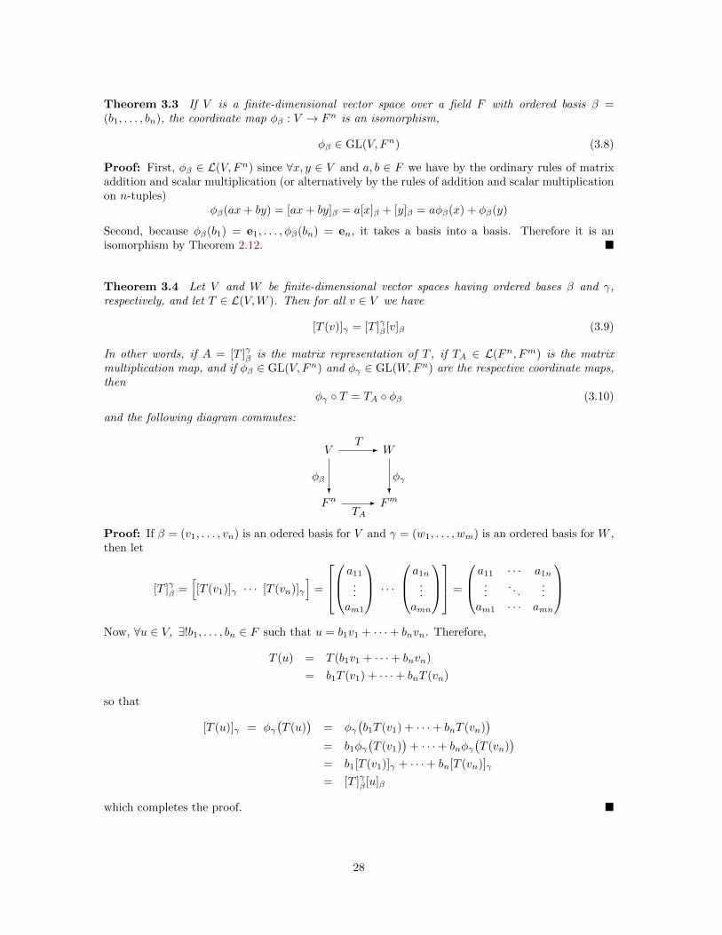
Theorem 3.4 Let V and W be finite-dimensional vector spaces having ordered bases β and γ,respectively, and let T ∈ L(V,W ). Then for all v ∈ V we have

[T (v)]γ = [T ]γβ [v]β (3.9)

In other words, if A = [T ]γβ is the matrix representation of T , if TA ∈ L(Fn, Fm) is the matrixmultiplication map, and if φβ ∈ GL(V, Fn) and φγ ∈ GL(W,Fn) are the respective coordinate maps,then

φγ ◦ T = TA ◦ φβ (3.10)

and the following diagram commutes:

VT - W

Fn

φβ?

TA- Fm

φγ?

Proof: If β = (v1, . . . , vn) is an odered basis for V and γ = (w1, . . . , wm) is an ordered basis for W ,then let

[T ]γβ =[[T (v1)]γ · · · [T (vn)]γ

]=

a11

...am1

· · ·a1n

...amn

=

a11 · · · a1n...

. . ....

am1 · · · amn

Now, ∀u ∈ V, ∃!b1, . . . , bn ∈ F such that u = b1v1 + · · ·+ bnvn. Therefore,

T (u) = T (b1v1 + · · ·+ bnvn)

= b1T (v1) + · · ·+ bnT (vn)

so that

[T (u)]γ = φγ(T (u)

)= φγ

(b1T (v1) + · · ·+ bnT (vn)

)= b1φγ

(T (v1)

)+ · · ·+ bnφγ

(T (vn)

)= b1[T (v1)]γ + · · ·+ bn[T (vn)]γ

= [T ]γβ [u]β

which completes the proof. �

28

Theorem 3.5 If V,W,Z are finite-dimensional vector spaces with ordered bases α, β and γ, re-spectively, and T ∈ L(V,W ) and U ∈ L(W,Z), then

[U ◦ T ]γα = [U ]γβ [T ]βα (3.11)

Proof: By the previous two theorems we have

[U ◦ T ]γα =[[(U ◦ T )(v1)]γ · · · [(U ◦ T )(vn)]γ

]=

[[U(T (v1))]γ · · · [U(T (vn))]γ

]=

[[U ]γβ [T (v1)]β · · · [U ]γβ [T (vn)]β

]= [U ]γβ

[[T (v1)]β · · · [T (vn)]β

]= [U ]γβ [T ]βα

which completes the proof. �

Corollary 3.6 If V is an n-dimensional vector space over F with an ordered basis β and I ∈ L(V )is the identity operator, then [I]β = In ∈Mn(F ).

Proof: By Theorem 3.5, given any T ∈ L(V ), T = I ◦T , so that [T ]β = [I ◦T ]β = [I]β [T ]β = In[T ]β ,so that [I]β = In by the cancellation law. �

Theorem 3.7 If V and W are finite-dimensional vector spaces of dimensions n and m, respectively,with ordered bases β and γ, respectively, and T ∈ L(V,W ), then

rank(T ) = rank([T ]γβ) and null(T ) = null([T ]γβ) (3.12)

Proof: This follows from Theorem 3.4, since φγ and φβ are isomorphisms, and so carry bases intobases, and φγ ◦ T = TA ◦ φβ , so that

rank(T ) = dim(im(T )

)= dim(φγ(im(T ))

)= rank(φγ ◦ T )

= rank(TA ◦ φβ) = dim(im(TA ◦ φβ))

)= dim

(im(TA)

)= rank(TA) = rank(A) = rank([T ]γβ)

while the second equality follows from the rank nullity theorem along with the fact that the ranksare equal. �

Theorem 3.8 If V and W are finite-dimensional vector spaces over F with ordered bases β =(b1, . . . , bn) and γ = (c1, . . . , cm), then the function

Φ : L(V,W )→Mm,n(F ) (3.13)

Φ(T ) = [T ]γβ (3.14)

is an isomorphism,Φ ∈ GL

(L(V,W ), Mm,n

)(3.15)

and consequentlyL(V,W ) ∼= Mm,n(F ) (3.16)

anddim

(L(V,W )

)= dim

(Mm,n(F )

)= mn (3.17)

29

Proof: First, Φ ∈ L(L(V,W ),Mm,n

): there exist scalars rij , sij ∈ F , for i = 1, . . . ,m and j =

1, . . . , n, such that for any T ∈ L(V,W ) we have

T (b1) = r11c1 + · · ·+ rm1cm

...

T (bn) = r1nc1 + · · ·+ rmncm

and

U(b1) = s11c1 + · · ·+ sm1cm

...

U(bn) = s1nc1 + · · ·+ smncm

Hence, for all k, l ∈ F and j = 1, . . . , n we have

(kT + lU)(bj) = kT (bj) + lU(bj) = k

m∑i=1

rijci + l

m∑i=1

sijci =

m∑i=1

(krij + lsij)ci

As a consequence of this and the rules of matrix addition and scalar multiplication we have

Φ(kT + lU) = [kT + lU ]γβ

=

kr11 + ls11 · · · kr1n + ls1n...

. . ....

krm1 + lsm1 · · · krmn + lsmn

= k

r11 · · · r1n...

. . ....

rm1 · · · rmn

+ l

s11 · · · s1n...

. . ....

sm1 · · · smn

= k[T ]γβ + l[U ]γβ= kΦ(T ) + lΦ(U)

Moreover, Φ is bijective by Theorem 2.5, since ∀A ∈ Mm,n, ∃!T ∈ L(V,W ) such that Φ(T ) = A,because there exists a unique T ∈ L(V,W ) such that

T (bj) = A1jc1 + · · ·+Anjcm for j = 1, . . . , n

This makes Φ onto, and also 1-1 because ker(Φ) = {T0} because for O ∈ Mm×n(F ) there is onlyT0 ∈ L(V,W ) such that Φ(T0) = O, because

T (bj) = 0c1 + · · ·+ 0cm = 0 for j = 1, . . . , n

defines a unique transformation, T0. �

Theorem 3.9 If V and W are finite-dimensional vector spaces over the same field F with orderedbases β = (b1, . . . , bn) and γ = (c1, . . . , cn), respectively, then T ∈ L(V,W ) is an isomporhpism iff[T ]γβ is invertible, in which case

[T−1]βγ =([T ]γβ

)−1(3.18)

Proof: If T is an isomorphism and dim(V ) = dim(W ) = n, then T−1 ∈ L(W,V ), and T ◦T−1 = IWand T−1 ◦ T = IV , so that by Theorem 3.5, Corollary 3.6 and Theorem 3.1 we have

[T ]γβ [T−1]βγ = [T ◦ T−1]γ = [IW ]γ = In = [IV ]β = [T−1 ◦ T ]β = [T−1]βγ [T ]γβ

so that [T ]γβ is invertibe with inverse [T−1]βγ , and by the uniqueness of the multiplicative inverse in

Mn(F ), which follows from the uniqueness of T−1A ∈ L(Fn), we have

[T−1]βγ =([T ]γβ

)−130

Conversely, if A = [T ]γβ is invertible, there is a n × n matrix B such that AB = BA = In, so by

Theorem 2.5 there is a unique U ∈ L(W,V ) such that U(cj) = vj =∑ni=1Bijbj . Hence B = [U ]βγ .

To show that U = T−1, note that

[U ◦ T ]β = [U ]βγ [T ]γβ = BA = In = [IV ]β and [T ◦ U ]γ = [T ]γβ [U ]βγ = AB = In = [IW ]γ

But since Φ ∈(L(V,W ),Mm,n(F )

)is an isomorphism, and therefore 1-1, we must have that

U ◦ T = IV and T ◦ U = IW

By the uniqueness of the inverse, however, U = T−1, and T is an isomorphism. �

31

4 Change of Coordinates

4.1 Definitions

We can also now define the change of coordinates or change of basis, operator. If V is afinite-dimensional vector space, say dim(V ) = n, and β = (b1, . . . , bn) and γ = (c1, . . . , cn) aretwo ordered bases for V , then the coordinate maps φβ , φγ ∈ L(V, Fn), which are isomorphisms byTheorem 2.15, may be used to define a change of coordinates operator φβ,γ ∈ L(Fn) changing βcoordinates into γ coordinates, that is having the property

φβ,γ([v]β) = [v]γ (4.1)

We define the operator byφβ,γ := φγ ◦ φ−1β (4.2)

The relationship between these three functions is illustrated in the following commutative diagram:

Fnφγ ◦ φ−1β - Fn

Vφγ

-

φβ

�

The change of coordinates operator has a matrix representation

Mβ,γ = [φβ,γ ]ρ = [φγ ]ρβ =[[b1]γ [b2]γ · · · [bn]γ

](4.3)

4.2 Change of Coordinate Maps and Matrices

Theorem 4.1 (Change of Coordinate Matrix) Let V be a finite-dimensional vector space overa field F and β = (b1, . . . , bn) and γ = (c1, . . . , cn) be two ordered bases for V . Since φβ and φγ areisomorphisms, the following diagram commutes,

Fnφγ ◦ φ−1β - Fn

Vφγ

-

φβ

�

and the change of basis operator φβ,γ := φγ◦φ−1β ∈ L(Fn), changing β coordinates into γ coordinates,is an automorphism of Fn. It’s matrix representation,

Mβ,γ = [φβ,γ ]ρ ∈Mn(F ) (4.4)

where ρ = (e1, . . . , en) is the standard ordered basis for Fn, is called the change of coordinatematrix, and it satisfies the following conditions:

1. Mβ,γ = [φβ,γ ]ρ

= [φγ ]ρβ

=[[b1]γ [b2]γ · · · [bn]γ

]2. [v]γ = Mβ,γ [v]β , ∀v ∈ V3. Mβ,γ is invertible and M−1β,γ = Mγ,β = [φβ ]ργ

32

Proof: The first point is shown as follows:

Mβ,γ = [φβ,γ ]ρ =[φβ,γ(e1) φβ,γ(e2) · · · φβ,γ(en)

]=

[(φγ ◦ φ−1β )(e1) (φγ ◦ φ−1β )(e2) · · · (φγ ◦ φ−1β )(en)

]=

[(φγ ◦ φ−1β )([b1]β) (φγ ◦ φ−1β )([b2]β) · · · (φγ ◦ φ−1β )([bn]β)

]=

[φγ(b1) φγ(b2) · · · φγ(bn)

]=

[[b1]γ [b2]γ · · · [bn]γ

]= [φγ ]β

or by Theorem 3.5 and Theorem 3.9 we have that

Mβ,γ = [φβ,γ ]ρ = [φγ ◦ φ−1β ]ρ = [φγ ]ρβ [φ−1β ]βρ = [φγ ]ργ([φβ ]ρβ)−1 = [φγ ]ρβI−1n = [φγ ]ρβIn = [φγ ]ρβ

The second point follows from Theorem 3.4, since

φγ(v) = (φγ ◦ I)(v) = (φγ ◦ (φ−1β ◦ φβ))(v) = ((φγ ◦ φ−1β ) ◦ φβ)(v)

implies that

[v]γ = [φγ(v)]ρ = [((φγ ◦ φ−1β ) ◦ φβ)(v)]ρ = [φγ ◦ φ−1β ]ρ[φβ(v)]ρ = [φβ,γ ]ρ[v]β = Mβ,γ [v]β

And the last point follows from the fact that φβ and φγ are isomorphism, so that φβ,γ is an isomor-phism, and hence φ−1β,γ ∈ L(Fn) is an isomorphism, and because the diagram above commutes wemust have

φ−1β,γ = (φγ ◦ φ−1β )−1 = φβ ◦ φ−1γ = φβ,γ

so that by 1M−1β,γ = [φ−1β,γ ]ρ = [φγ,β ]ρ = Mγ,β

or alternatively by Theorem 3.9

M−1β,γ = ([φβ,γ ]ρ)−1 = [φ−1β,γ ]ρ = [φγ,β ]ρ = [φβ ]ργ = Mγ,β �

Corollary 4.2 (Change of Basis) Let V and W be finite-dimensional vector spaces over the samefield F and let (β, γ) and (β′, γ′) be pairs of ordered bases for V and W , respectively. If T ∈ L(V,W ),then

[T ]γ′

β′ = Mγ,γ′ [T ]γβMβ′,β (4.5)

= Mγ,γ′ [T ]γβM−1β,β′ (4.6)

where Mγ,γ′ and Mβ′,β are change of coordinate matrices. That is, the following diagram commutes

FnTA - Fn

FnTA′-

φβ,β′

-

Fn

φγ′,γ

�

V

φβ′6

T-

φβ

�

W

φγ′6

φγ

-

33

Proof: This follows from the fact that if β = (b1, . . . , bn), β′ = (b′1, . . . , b′n), γ = (c1, . . . , cm),

γ = (c′1, . . . , c′m), then for each i = 1, . . . , n we have

[T (b′i)]γ′ = [(φγ,γ′ ◦ T ◦ φ−1β,β′)(b′i)]γ′

so

[T ]γ′

β′ = [φγ,γ′ ◦ T ◦ φ−1β,β′ ]γ′

β′

= [φγ,γ′ ]ρm [T ]γβ [φ−1β,β′ ]ρn

= [φγ,γ′ ]ρm [T ]γβ([φβ,β′ ]ρn)−1

= Mγ,γ′ [T ]γβM−1β,β′

which completes the proof. �

Corollary 4.3 (Change of Basis for a Linear Operator) If V is a finite-dimensional vectorspace with ordered bases β and γ, and T ∈ L(V ), then

[T ]γ = Mβ,γ [T ]βM−1β,γ (4.7)

where Mβ,γ is the change of coordinates matrix. �

Corollary 4.4 If we are given any two of the following:

(1) A ∈Mn(F ) invertible

(2) an ordered basis β for Fn

(3) an ordered basis γ for Fn

the third is uniquely determined by the equation A = Mβ,γ , where Mβ,γ is the change of coordinatesmatrix of the previous theorem.

Proof: If we have A = Mβ,γ = [φβ ]γ =[[b1]γ [b2]γ · · · [bn]γ

], suppose we know A and γ. Then,

[bi]γ is given by A, so bi = Ai1c1 + · · · + Aincn, so β is uniquely determined. If β and γ are given,

then by the previous theorem Mβ,γ is given by Mβ,γ =[[b1]γ [b2]γ · · · [bn]γ

]. Lastly, if A and β

are given, then γ is given by the first case applied to A−1 = Mγ,β . �

34