abstract wide-area mobile content delivery bo han, doctor of

ABSTRACT

Title of dissertation: WIDE-AREA MOBILE CONTENT DELIVERY

Bo Han, Doctor of Philosophy, 2012

Dissertation directed by: Professor Aravind SrinivasanDepartment of Computer ScienceandProfessor Bobby BhattacharjeeDepartment of Computer Science

Hybrid mobile content delivery systems improve performance of wide-area net-

works by combining both wide-area and local-area communications. In hybrid con-

tent delivery, service providers send data packets first to a small number of selected

users (e.g., those with good channel quality) and then these mobile users help for-

ward the packets to others (e.g., those with poor channel quality). The central

theme of our work is to identify the initial target set composed of influential mobile

users (i.e., individuals with high centrality in their social-contact graphs) and thus

improve the efficiency of hybrid mobile content distribution.

We first present two centralized algorithms for this target-set selection prob-

lem. The greedy algorithm has a provable performance guarantee, due to the sub-

modularity of the underlying information dissemination function. The heuristic

algorithm exploits the regularity of human mobility and is more practical than the

greedy algorithm. We then propose a lightweight and distributed protocol to iden-

tify these influential users through random-walk sampling. This distributed protocol

leverages random-walk probe messages to sample mobile users and estimates their

centrality based on how many times they are visited by the probe messages. This

protocol has low communication and computation overhead and lends itself well to

mobile content delivery. We verify the effectiveness of these approaches through

extensive trace-driven simulation studies using real-world mobility traces.

WIDE-AREA MOBILE CONTENT DELIVERY

by

Bo Han

Dissertation submitted to the Faculty of the Graduate School of theUniversity of Maryland, College Park in partial fulfillment

of the requirements for the degree ofDoctor of Philosophy

2012

Advisory Committee:Professor Aravind Srinivasan, Chair/AdvisorProfessor Bobby Bhattacharjee, Co-Chair/Co-AdvisorProfessor Richard J. La, Dean’s RepresentativeProfessor Amol DeshpandeProfessor Jennifer Golbeck

c© Copyright by

Bo Han2012

Dedication

To my family.

ii

Acknowledgments

First and foremost, I would like to thank my advisors, Aravind Srinivasan and

Bobby Bhattacharjee. I am deeply indebted to them for their invaluable guidance,

support and encouragement. Aravind has guided me on almost all things, including

identifying and approaching research problems, preparing papers and slides, job

searching and interviewing. He always encourages me to think big and then focus on

important problems. Bobby has brought me into the systems research and offered

me the freedom to work on topics that interested me. I am very grateful for his

help on shaping my attitude and ability towards research and work. I also want to

show my sincere gratitude to my dissertation committee members, Amol Deshpande,

Jennifer Golbeck and Richard La, for their support and feedback.

I owe a lot to Robert Miller and Lusheng Ji for their constant guidance and

encouragement throughout my graduate life. They introduced me to several prac-

tical problems of 802.11 WLANs and offered me three internship opportunities. It

has been a wonderful journey for me since I met Robert and Lusheng at AT&T Labs

Research, and they have been great mentors ever since. Fortunately, I will continue

to work with them after graduation.

I am grateful to my long-term collaborators, Madhav Marathe and Anil Vul-

likanti. They introduced me to the scheduling problems in wireless networks, shared

with me the mobility traces, and invited me to visit Virginia Tech. I was also ex-

tremely fortunate to work with Francesco Gringoli from the University of Brescia.

I learnt a lot from him about how to program the firmware of Broadcom chipsets.

iii

His work attitude always inspires me to pursue the best and go beyond that.

I thank Tianji Li and Katherine Guo for reviewing my job application mate-

rials and their comments about my job talk. I would also like to thank my other

collaborators/coauthors during the graduate study: Suman Banerjee, Luca Com-

inardi, Savio Dimatteo, Pan Hui, Pete Keleher, Seungjoon Lee, Dave Levin, Jian

Li, Victor O. K. Li, Cristian Lumezanu, Lorenzo Nava, Srinivasan Parthasarathy,

Guanhong Pei, Aaron Schulman, Jianhua Shao and Neil Spring.

I want to thank my friends Kan-Leung Cheng, Ran Liu, Shanchan Wu and

Xiaoyu Zhang for their help and stimulating discussions during my graduate life. I

also thank the technical and administrative staff of the department for their support.

Last but not least, my thanks go to my family – my parents, my wife, and my

sister – for their unconditional love.

iv

Table of Contents

List of Tables vii

List of Figures viii

1 Introduction 11.1 Mobile Content Delivery and Its Challenges . . . . . . . . . . . . . . 11.2 Our Contributions . . . . . . . . . . . . . . . . . . . . . . . . . . . . 4

2 Related Work 82.1 Mobile Content Delivery/Dissemination . . . . . . . . . . . . . . . . . 8

2.1.1 Cellular Multicast Systems . . . . . . . . . . . . . . . . . . . . 82.1.2 Hybrid Content Delivery . . . . . . . . . . . . . . . . . . . . . 92.1.3 Opportunistic Information Dissemination . . . . . . . . . . . . 9

2.2 Identifying Influential Users . . . . . . . . . . . . . . . . . . . . . . . 112.2.1 Traditional Social Networks . . . . . . . . . . . . . . . . . . . 112.2.2 Wireless Mobile Networks . . . . . . . . . . . . . . . . . . . . 122.2.3 Targeted Immunization . . . . . . . . . . . . . . . . . . . . . . 12

2.3 Random Walk And Its Applications . . . . . . . . . . . . . . . . . . . 132.4 Mobile Social Networks . . . . . . . . . . . . . . . . . . . . . . . . . . 15

3 Background of Wireless Networks – Bit Error Patterns 173.1 Introduction . . . . . . . . . . . . . . . . . . . . . . . . . . . . . . . . 173.2 IEEE 802.11 Wireless LAN Communications . . . . . . . . . . . . . . 193.3 Experimental Platform . . . . . . . . . . . . . . . . . . . . . . . . . . 22

3.3.1 Hardware Configuration . . . . . . . . . . . . . . . . . . . . . 223.3.2 RSSI Calibration . . . . . . . . . . . . . . . . . . . . . . . . . 233.3.3 Experimental Procedure . . . . . . . . . . . . . . . . . . . . . 25

3.4 Experiments and Results . . . . . . . . . . . . . . . . . . . . . . . . . 293.4.1 Overview . . . . . . . . . . . . . . . . . . . . . . . . . . . . . 293.4.2 Bit Error Distribution Patterns . . . . . . . . . . . . . . . . . 313.4.3 Quantification of Patterns . . . . . . . . . . . . . . . . . . . . 353.4.4 Different Physical Environments . . . . . . . . . . . . . . . . . 37

3.4.4.1 Emulab Wireless Testbed . . . . . . . . . . . . . . . 383.4.4.2 Shielded Room . . . . . . . . . . . . . . . . . . . . . 383.4.4.3 Cable . . . . . . . . . . . . . . . . . . . . . . . . . . 40

3.4.5 Different Hardware Platforms . . . . . . . . . . . . . . . . . . 413.4.5.1 Atheros AR5006 Receiver . . . . . . . . . . . . . . . 423.4.5.2 Broadcom Receiver . . . . . . . . . . . . . . . . . . . 453.4.5.3 Atheros AR9285 Receiver . . . . . . . . . . . . . . . 483.4.5.4 Intel Receiver . . . . . . . . . . . . . . . . . . . . . . 48

3.4.6 Different Modulation . . . . . . . . . . . . . . . . . . . . . . . 503.4.7 Challenged 802.11 Environments . . . . . . . . . . . . . . . . 503.4.8 Real Traces . . . . . . . . . . . . . . . . . . . . . . . . . . . . 54

v

3.4.9 Summary . . . . . . . . . . . . . . . . . . . . . . . . . . . . . 563.5 Hypotheses and Discussions . . . . . . . . . . . . . . . . . . . . . . . 57

4 Centralized Target Set Selection 614.1 Introduction . . . . . . . . . . . . . . . . . . . . . . . . . . . . . . . . 614.2 Submodularity of Information Dissemination Function . . . . . . . . . 664.3 Greedy and Heuristic Algorithms . . . . . . . . . . . . . . . . . . . . 694.4 Simulation Studies . . . . . . . . . . . . . . . . . . . . . . . . . . . . 71

4.4.1 Mobility Traces . . . . . . . . . . . . . . . . . . . . . . . . . . 714.4.1.1 Synthetic Mobility Trace . . . . . . . . . . . . . . . . 714.4.1.2 Traces From Real-World Experiments . . . . . . . . 72

4.4.2 Simulation Results . . . . . . . . . . . . . . . . . . . . . . . . 744.4.2.1 Pull Probability . . . . . . . . . . . . . . . . . . . . . 754.4.2.2 Delay-Tolerance Threshold . . . . . . . . . . . . . . . 774.4.2.3 Another Synthetic Mobility Trace . . . . . . . . . . . 784.4.2.4 Comparing Random, Heuristic, and Greedy . . . . . 78

5 Random-Walk Based Sampling 855.1 Introduction . . . . . . . . . . . . . . . . . . . . . . . . . . . . . . . . 855.2 Probabilistic Temporal Graphs . . . . . . . . . . . . . . . . . . . . . . 865.3 The Random-Walk Sampling Protocol . . . . . . . . . . . . . . . . . 89

5.3.1 The Protocol . . . . . . . . . . . . . . . . . . . . . . . . . . . 895.3.2 Theoretical Analysis . . . . . . . . . . . . . . . . . . . . . . . 915.3.3 Proof of Concept . . . . . . . . . . . . . . . . . . . . . . . . . 95

5.4 Facilitating Mobile Content Delivery . . . . . . . . . . . . . . . . . . 975.4.1 Target-Set Selection Using Random Walks . . . . . . . . . . . 975.4.2 Performance Evaluation . . . . . . . . . . . . . . . . . . . . . 98

5.4.2.1 Simulation Setup . . . . . . . . . . . . . . . . . . . . 995.4.2.2 The Amount of Cellular Data Traffic . . . . . . . . . 1005.4.2.3 Delivery Delay . . . . . . . . . . . . . . . . . . . . . 104

5.5 Controlling Infectious Diseases . . . . . . . . . . . . . . . . . . . . . . 1065.5.1 Random-Walk Based Immunization . . . . . . . . . . . . . . . 1065.5.2 Performance Evaluation . . . . . . . . . . . . . . . . . . . . . 107

5.5.2.1 Simulation Setup . . . . . . . . . . . . . . . . . . . . 1075.5.2.2 Targeted Immunization . . . . . . . . . . . . . . . . 1095.5.2.3 Effects of Various Random-Walk Parameters . . . . . 1135.5.2.4 Early Detection of Outbreaks . . . . . . . . . . . . . 116

6 Conclusions and Future Work 1196.1 What We Have Done . . . . . . . . . . . . . . . . . . . . . . . . . . . 1196.2 Unaddressed Issues . . . . . . . . . . . . . . . . . . . . . . . . . . . . 1206.3 Future Directions . . . . . . . . . . . . . . . . . . . . . . . . . . . . . 122

Bibliography 124

vi

List of Tables

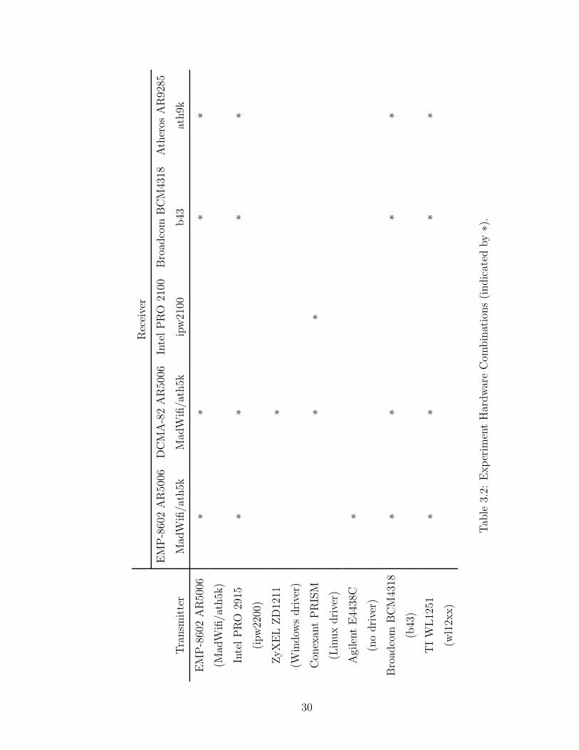
3.1 IEEE 802.11 PHY Parameters. . . . . . . . . . . . . . . . . . . . . . 203.2 Experiment Hardware Combinations (indicated by ∗). . . . . . . . . . 303.3 The slopes and intercepts of the fitting lines, and the calculated pe-

riods of the fitting saw-lines. . . . . . . . . . . . . . . . . . . . . . . . 373.4 Finger Width. . . . . . . . . . . . . . . . . . . . . . . . . . . . . . . . 37

4.1 The start time of three selected 1-hour periods from INFOCOM06trace. . . . . . . . . . . . . . . . . . . . . . . . . . . . . . . . . . . . . 73

4.2 The start time of three selected 6-hour periods from Reality Miningtrace. . . . . . . . . . . . . . . . . . . . . . . . . . . . . . . . . . . . . 73

4.3 The top 5 most active users for different periods and the expectednumber users that they can infect. . . . . . . . . . . . . . . . . . . . . 80

4.4 Summary of two real-world traces. . . . . . . . . . . . . . . . . . . . . 81

5.1 The power level of Bluetooth and WiFi on Nokia N900 during dis-covery and idle modes (in mW). . . . . . . . . . . . . . . . . . . . . . 96

vii

List of Figures

3.1 IEEE 802.11 bit stream encoding process for OFDM modulation. . . 223.2 Calibration setup. . . . . . . . . . . . . . . . . . . . . . . . . . . . . . 243.3 Boonton 4400 Power Meter Display. . . . . . . . . . . . . . . . . . . . 253.4 RSSI to received signal power mapping. The slope of the fitting line

is 1.002 with 95% confidence bounds (0.96, 1.044). . . . . . . . . . . . 263.5 Primary testbed topology. . . . . . . . . . . . . . . . . . . . . . . . . 283.6 Normalized bit error frequency, over the total number of received

error packets, for node 3; bit rate set to 54 Mbps. . . . . . . . . . . . 323.7 Normalized bit error frequency for node 4 with bit rate 54 Mbps. The

average RSSIs of correct packets, truncated packets and packets withbit errors are 36, 21 and 22, respectively. . . . . . . . . . . . . . . . . 33

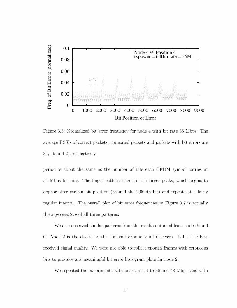
3.8 Normalized bit error frequency for node 4 with bit rate 36 Mbps. Theaverage RSSIs of correct packets, truncated packets and packets withbit errors are 34, 19 and 21, respectively. . . . . . . . . . . . . . . . . 34

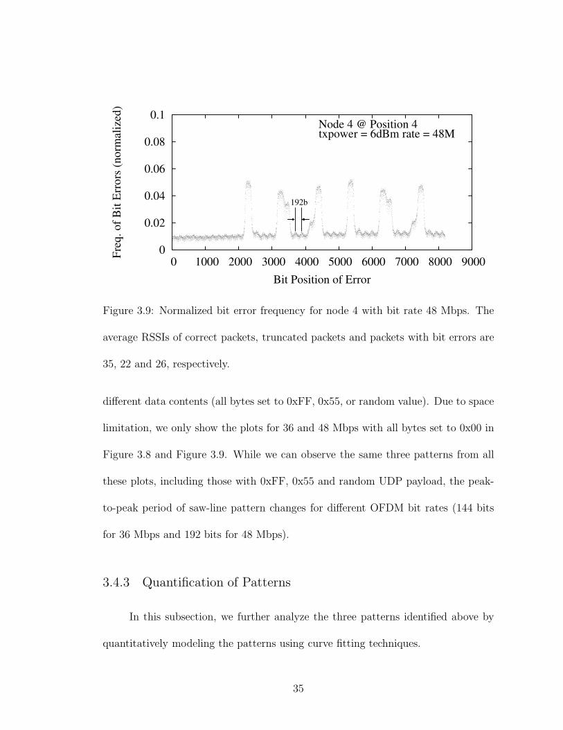
3.9 Normalized bit error frequency for node 4 with bit rate 48 Mbps. Theaverage RSSIs of correct packets, truncated packets and packets withbit errors are 35, 22 and 26, respectively. . . . . . . . . . . . . . . . . 35

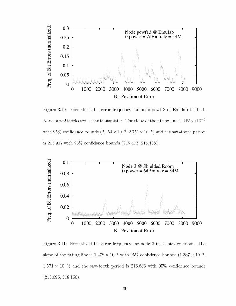
3.10 Normalized bit error frequency for node pcwf13 of Emulab testbed.Node pcwf2 is selected as the transmitter. The slope of the fitting lineis 2.553×10−6 with 95% confidence bounds (2.354×10−6, 2.751×10−6)and the saw-tooth period is 215.917 with 95% confidence bounds(215.473, 216.438). . . . . . . . . . . . . . . . . . . . . . . . . . . . . 39

3.11 Normalized bit error frequency for node 3 in a shielded room. Theslope of the fitting line is 1.478 × 10−6 with 95% confidence bounds(1.387×10−6, 1.571×10−6) and the saw-tooth period is 216.886 with95% confidence bounds (215.695, 218.166). . . . . . . . . . . . . . . . 39

3.12 Normalized bit error frequency for over the cable communication. Theslope of the fitting line is 4.720 × 10−7 with 95% confidence bounds(3.849×10−7, 5.591×10−7) and the saw-tooth period is 216.512 with95% confidence bounds (216.066, 216.961). . . . . . . . . . . . . . . . 41

3.13 Normalized bit error frequency for ZyXEL ZyDAS ZD1211 to DCMAAtheros AR5006. The slope of the fitting line is 2.434 × 10−6 with95% confidence bounds (2.323×10−6, 2.544×10−6) and the saw-toothperiod is 216.289 with 95% confidence bounds (215.030, 217.637). . . 43

3.14 Normalized bit error frequency for Conexant PRISM to DCMA AtherosAR5006. The slope of the fitting line is 2.575 × 10−6 with 95% con-fidence bounds (2.479 × 10−6, 2.670 × 10−6). The saw-line patternin this figure is not clear enough to perform curve fitting and thesaw-tooth period inferred from the fingers is 207.8. . . . . . . . . . . 43

viii

3.15 Normalized bit error frequency for Agilent signal generator to EMPAtheros AR5006. The slope of the fitting line is 3.165 × 10−7 with95% confidence bounds (2.410×10−7, 3.921×10−7) and the saw-toothperiod is 217.487 with 95% confidence bounds (212.845, 222.414). . . 44

3.16 Normalized bit error frequency for Intel PRO 2915 to DCMA AtherosAR5006. The slope of the fitting line is 1.286× 10−6 with 95% confi-dence bounds (1.276× 10−6, 1.297 × 10−6) and the saw-tooth periodis 217.487 with 95% confidence bounds (216.512, 218.394). . . . . . . 44

3.17 Normalized bit error frequency for Broadcom BCM4318 to BroadcomBCM4318. The slope of the fitting line is 6.506 × 10−6 with 95%confidence bounds (6.444 × 10−6, 6.572 × 10−6) and the saw-toothperiod is 216.066 with 95% confidence bounds (215.917, 216.140). . . 46

3.18 Normalized bit error frequency for EMP Atheros AR5006 to Broad-com BCM4318. The slope of the fitting line is 1.022×10−5 with 95%confidence bounds (1.016 × 10−5, 1.027 × 10−5) and the saw-toothperiod is 215.843 with 95% confidence bounds (215.769, 215.917). . . 46

3.19 Normalized bit error frequency for Intel PRO 2915 to BroadcomBCM4318. The slope of the fitting line is 1.638 × 10−5 with 95%confidence bounds (1.624 × 10−5, 1.653 × 10−5) and the saw-toothperiod is 215.769 with 95% confidence bounds (215.769, 215.843). . . 47

3.20 Normalized bit error frequency for EMP Atheros AR5006 to AtherosAR9285. The slope of the fitting line is 1.970× 10−5 with 95% confi-dence bounds (1.965× 10−5, 1.975 × 10−5) and the saw-tooth periodis 215.769 with 95% confidence bounds (215.695, 215.917). . . . . . . 47

3.21 Normalized bit error frequency for Intel PRO 2915 to Atheros AR9285.The slope of the fitting line is 1.935×10−6 with 95% confidence bounds(1.908×10−6, 1.961×10−6) and the saw-tooth period is 216.289 with95% confidence bounds (216.140, 216.363). . . . . . . . . . . . . . . . 49

3.22 Normalized bit error frequency for Broadcom BCM4318 to AtherosAR9285. The slope of the fitting line is 6.628× 10−6 with 95% confi-dence bounds (6.555× 10−6, 6.701 × 10−6) and the saw-tooth periodis 218.546 with 95% confidence bounds (216.438, 220.617). . . . . . . 49

3.23 Normalized bit error frequency for node 4 using IEEE 802.11b. Theslope of the fitting line is 4.224 × 10−7 with 95% confidence bounds(4.174 × 10−7, 4.274 × 10−7) and the saw-tooth period is 72.014 (9symbol lengths of DSSS CCK) with 95% confidence bounds (71.997,72.030). . . . . . . . . . . . . . . . . . . . . . . . . . . . . . . . . . . 51

3.24 Normalized bit error frequency for Conexant PRISM to Intel PRO2100. The slope of the fitting line is 1.288×10−6 with 95% confidencebounds (1.275 × 10−6, 1.301 × 10−6). . . . . . . . . . . . . . . . . . . 51

3.25 The mobile testbed in a hallway. During the experiments, we walkbetween A and B with the smartphone transmitter in hand. . . . . . 52

ix

3.26 Normalized bit error frequency for TI WL1251 to Atheros AR9285,mobile environment. The slope of the fitting line is 3.925×10−6 with95% confidence bounds (3.893×10−6, 3.957×10−6) and the saw-toothperiod is 215.769 with 95% confidence bounds (215.695, 215.917). . . 53

3.27 Normalized bit error frequency for TI WL1251 to Atheros AR9285,outdoor environment. The slope of the fitting line is 4.676 × 10−6

with 95% confidence bounds (4.551 × 10−6, 4.801 × 10−6) and thesaw-tooth period is 215.917 with 95% confidence bounds (215.843,215.991). . . . . . . . . . . . . . . . . . . . . . . . . . . . . . . . . . . 53

3.28 Normalized bit error frequency for TI WL1251 to DCMA AtherosAR5006, mobile environment. The slope of the fitting line is 1.771×10−6 with 95% confidence bounds (1.728 × 10−6, 1.815 × 10−6) andthe saw-tooth period is 215.473 with 95% confidence bounds (214.443,216.587). . . . . . . . . . . . . . . . . . . . . . . . . . . . . . . . . . . 55

3.29 Normalized bit error frequency for EMP Atheros AR5006 to DCMAAtheros AR5006 using real traces. The slope of the fitting line is2.316×10−6 with 95% confidence bounds (2.286×10−6, 2.346×10−6)and the saw-tooth period is 214.957 with 95% confidence bounds(214.370, 215.547). . . . . . . . . . . . . . . . . . . . . . . . . . . . . 55

4.1 A snapshot of the contact graph for a small group of subscribed mobileusers. . . . . . . . . . . . . . . . . . . . . . . . . . . . . . . . . . . . . 63

4.2 The social graph of mobile users shown in Figure 4.1. . . . . . . . . . 634.3 Performance of Random algorithm for different pull probabilities (Port-

land city data set). . . . . . . . . . . . . . . . . . . . . . . . . . . . . 764.4 Performance of Random algorithm for different delay-tolerance thresh-

olds (Portland city data set). . . . . . . . . . . . . . . . . . . . . . . . 764.5 Performance of Random algorithm for different pull probabilities (Utah

state data set). . . . . . . . . . . . . . . . . . . . . . . . . . . . . . . 794.6 Performance of Random algorithm for different delay-tolerance thresh-

olds (Utah state data set). . . . . . . . . . . . . . . . . . . . . . . . . 794.7 Performance comparison of Random, Heuristic, and Greedy algo-

rithms for the INFOCOM06 data set. . . . . . . . . . . . . . . . . . . 834.8 Performance comparison of Random, Heuristic, and Greedy algo-

rithms for the Reality Mining data set. . . . . . . . . . . . . . . . . . 83

5.1 The social-contact graph for information exchange of three users, Al-ice, Bob and Carol. The durations of these three contacts are 50, 10and 2 minutes with pe 0.01, 0.005 and 0.001. . . . . . . . . . . . . . . 89

5.2 Comparison of the normalized cellular data traffic for four target-setselection schemes with different values of p. . . . . . . . . . . . . . . . 101

5.3 Comparison of the normalized cellular data traffic for three target-set selection schemes with different values of p. Only target users canpropagate information to others. . . . . . . . . . . . . . . . . . . . . . 103

x

5.4 Comparison of delivery delay for 4 target-set selection schemes withdifferent values of p. . . . . . . . . . . . . . . . . . . . . . . . . . . . 105

5.5 Comparison of the evolution of infected individuals for three im-munization policies, random, degree-based, and random-walk-based,with different infection probabilities, immunization start conditions,and initial infections. . . . . . . . . . . . . . . . . . . . . . . . . . . . 111

5.6 Comparison of random-walk based immunizations with different lengths,probabilities and frequencies. . . . . . . . . . . . . . . . . . . . . . . . 114

5.7 Comparison of the amount of per-user control messages for differentlengths, probabilities and frequencies of random walks. The numberof per-user control messages for the degree-based scheme ranges from1,441 to 25,608. . . . . . . . . . . . . . . . . . . . . . . . . . . . . . . 115

5.8 Comparison of early detection of outbreaks with randomly selectedmonitors and those selected using RW-10. . . . . . . . . . . . . . . . . 117

xi

Chapter 1

Introduction

1.1 Mobile Content Delivery and Its Challenges

One-to-many group communication is useful in mobile systems, such as de-

livery of regional content (e.g., multimedia newspaper) to subscribed users, traffic

map with congestion information, mobile advertising, and distribution of software

patches. Multicast seems to be an attractive solution for the group-based communi-

cations. However, the data rates of cellular multicast are low (e.g., 10 to 384 Kbps

for 3GPP MBMS – Multimedia Broadcast Multicast Service [1], and 38.4 to 2457.6

Kbps for 3GPP2 BCMCS – BroadCast MultiCast Service [2]). 802.11 uses 1 Mbps,

the lowest data rate, for multicast traffic.

Application layer multicast [7, 17] is a potential solution. However, there is no

good solution when using only cellular networks, because unicast content forwarding

through cellular networks still cannot address the low-throughput problem for users

with poor channel quality. Modern mobile devices have cellular, WiFi and Bluetooth

radios, and a possible solution is to consider a hybrid delivery model that combines

the local-area peer-to-peer and wide-area cellular communications.

In this dissertation, we investigate the performance of hybrid mobile content

delivery systems which work as follows. At the beginning, service providers send

the delivered content to only a small number of selected target users. Then dur-

1

ing their movement, the application running on their mobile devices will forward

the content to others through mobile-to-mobile opportunistic communications using

either Bluetooth or WiFi. Finally, service providers send (over cellular networks)

the content to users who cannot receive it (through opportunistic communications)

before the delivery deadline.

The central theme of our work is to identify influential target users for mobile

content distribution networks. If these target users can forward the delivered content

to a large number of mobile users through opportunistic communications, we can

offer high-throughput delivery for most users and potentially reduce the data traffic

over cellular networks. The hypothesis we want to verify is:

Given multi-mode radio stations and the limitations of pure multicast/unicast,

can high centrality users improve the performance of hybrid mobile content

delivery?

In contrast to existing approaches that first send content to users with good

channel quality [11, 56], we propose to identify these target users by considering their

centrality in the social-contact graph. The centrality of mobile users is affected by

their mobility and not all mobile users are equal in terms of mobility. Some of them,

such as salespeople, may travel to many places during a day, while others, such as

graduate students, may stay in their office for most of the working time. When

considering the problem of content dissemination in mobile networks, if we employ

these active salespeople as the initial physical carriers, they may be able to forward

the delivered content to a much larger fraction of mobile users, compared with

2

selecting initial carriers randomly. This is exactly the rationale behind the influence

maximization problem of information diffusion in traditional social networks [19, 45].

There is a trade-off between the accuracy of measured centrality and the com-

munication overhead. With the complete social-contact graph of mobile users, cen-

tralized algorithms can apply well-known metrics, such as degree centrality, closeness

centrality and betweenness centrality, to identify the intital target users. However,

mobile devices need to periodically send the updates of social-contact graphs to

centralized servers which will increase the communication overhead and thus may

not be energy efficient for mobile devices. Distributed protocols may reduce the

communication overhead by sending only a small amount of sampled data to cen-

tralized servers, but the accuracy of measured centrality may not be as good as their

centralized counterparts. We investigate the pros and cons of both centralized and

distributed solutions for the target-set selection problem in mobile content delivery

systems.

Another challenging issue of centrality estimation of mobile users is that we

should take privacy and energy consumption into account. We need to provide users

with opt-in and out options of content forwarding and they will act as relays only

when they participate in the hybrid content delivery system. The proposed solutions

should require only the contact information among users and should not track mobile

users’ locations. Moreover, they should consider the energy consumption of different

wireless interfaces when selecting the underlying communication technology, because

mobile devices are supported by batteries.

Our scheme is orthogonal to the existing solutions that consider mainly the

3

channel quality of mobile users. Technically, a base station can send the delivered

content to high centrality mobile users only when they have good channel quality.

Given the high centrality of these users, they may not always stay at areas with

poor channel quality.

1.2 Our Contributions

We make several contributions in this dissertation work to improve the effi-

ciency of mobile content delivery.

• We investigate the target-set selection problem in hybrid mobile content de-

livery systems. A target set is composed of influential mobile users with high

centrality in the social-contact graph. We use this target set as the initial set

of users who receive the delivered content from service providers without any

delay. These users then act as relays and forward the content to others during

their movement.

• We prove that the information dissemination function is submodular for the

contact graph of mobile users, which changes dynamically over time. The

proof is an extension of the result of Kempe, Kleinberg, and Tardos [45]. An

information dissemination function maps the initial target set to the expected

number of users who can receive the content before the delivery deadline. It

follows from the work of Nemhauser et al. [65] that if the information dissem-

ination function is submodular, a greedy algorithm for the target-set selection

problem can achieve a provable approximation ratio of (1 − 1/e) (the best

4

known result so far), where e is the base of the natural logarithm.

• We also propose a heuristic algorithm by exploiting the regularity of human

mobility [34, 58]. This algorithm leverages the greedy algorithm to identify

target users based on history mobility information and then applies this target

set for future content delivery. The heuristic algorithm is more practical than

the greedy algorithm because it does not require the knowledge of user mobility

in the future.

• We design a distributed and lightweight protocol to identify the influential in-

dividuals in hybrid mobile content delivery. The key idea behind this protocol

is to sample users through random-walk probe messages generated period-

ically by mobile devices and estimate the centrality of individuals through

their random-walk counters (i.e., how many times their mobile devices are

visited by the probe messages). To verify the feasibility of our proposed dis-

tributed protocol, we implement a proof-of-concept prototype on Nokia N900

smartphones.

• We prove that for static graphs that are “expander-like” (see, e.g., Eubank

et al. [24]), the nodes with high random-walk counters are very likely to be

those with high degrees. Our networks are inherently mobile and thus not

static, but their static snapshots will likely be expander-like. Mobile networks

will also likely mix well, serving to explain intriguing results such as those

of Grossglauser and Tse [36]. We emphasize that our proposed approaches

themselves (both centralized and distributed) are for dynamic social-contact

5

graphs.

• We evaluate the performance of a hybrid content delivery system which chooses

target users based on the random-walk counters of mobile users. Surprisingly,

we find that if we choose all target users with high centrality, the resultant

scheme performs better than a random-selection approach only for small target

sets. We also propose another enhanced scheme that chooses both influential

and non-influential users into the target set. Our simulation results verify

that this enhanced scheme outperforms random selection for large target sets.

Moreover, we demonstrate that the centrality information provided by our

random-walk sampling protocol is also useful for a targeted immunization

policy which vaccinates high-centrality users first to contain the spread of

infectious diseases.

• We study the sub-frame bit error patterns of 802.11 transmission to provide

a background of wireless communications. We construct a number of IEEE

802.11 WLAN testbeds and conduct extensive experiments to study the char-

acteristics of bit errors and their location distribution. Our measurement

results identify three bit error patterns: the slope-line, saw-line and finger pat-

terns. Among these three patterns, we verify that the slope-line and saw-line

patterns are present in WLAN transmissions in different physical environments

and across different WLAN hardware platforms.

This dissertation is organized as follows. We review related work in Chapter 2.

In Chapter 3, we present our experimental studies about sub-frame level bit error

6

patterns of wireless communications which offer a background of wireless networks.

We present two centralized algorithms for the target-set selection problem in hybrid

mobile content delivery in Chapter 4. In Chapter 5, we design a distributed protocol

with low communication overhead to identify the influential mobile users through

random-walk sampling. We conclude and discuss the future work in Chapter 6.

7

Chapter 2

Related Work

We review related work on mobile content distribution systems, identifying

influential individuals in various networks, applications of random walks and the

emerging mobile social networks in this chapter.

2.1 Mobile Content Delivery/Dissemination

2.1.1 Cellular Multicast Systems

There are a number of standards developed to provide multicast service for cel-

lular networks, for example, MBMS for 3GPP and BCMCS for 3GPP2. Since a base

station needs to use the same data rate to serve users in the same multicast group

with different channel conditions, the supported data rates of cellular multicast are

usually low [1, 2]. To solve this problem, Won et al. [89] propose two adaptive mul-

ticast scheduling algorithms to provide proportional fairness among mobile devices.

These algorithms support different utility functions for different scenarios depending

on the upper layer models of service providers. Kozat [50] investigates the through-

put performance of opportunistic multicast by considering multiuser diversity and

rateless erasure codes. Compared with the work that aims to improve the perfor-

mance cellular multicast itself, we study how to select influential mobile users who

can relay the multicast packets to others using local-area communications.

8

2.1.2 Hybrid Content Delivery

Hybrid content delivery that leverages both wide-area cellular and local-area

peer-to-peer communications has been studied to improve the efficiency of cellular

networks. Luo et al. [56] propose UCAN, the Unified Cellular and Ad-Hoc Network

architecture, to enhance the throughput of 3G networks, by forwarding packets to

mobile devices with poor channel quality through those with better channel qual-

ity. They develop various protocols for refined 3G base station scheduling, ad-hoc

routing, proxy discovery and secure crediting. Bhatia et al. [11] propose ICAM, a

system that integrates cellular and ad-hoc multicast, to increase the throughput of

3G multicast. They design a polynomial-time approximation algorithm with prov-

able performance guarantee. Goemans et al. [32] investigate the Nash equilibria

of various market sharing games for the problem of offloading 3G traffic to ad-hoc

networks. They propose a protocol that enables distributed caching and design in-

centive mechanisms that prevent selfish players from colluding. Differently from the

above work, we propose to send mobile content to users with high centrality in their

social-contact graph, instead of those with good channel quality.

2.1.3 Opportunistic Information Dissemination

There are also several existing works for information dissemination in wire-

less networks. 7DS [71] is a peer-to-peer data dissemination and sharing system for

mobile devices, aiming at increasing the data availability for users who have inter-

mittent connectivity. Due to the heterogeneity of access methods and the spatial

9

locality of information, when mobile devices fail to access Internet through their own

connections, they can try to query data from peers in their proximity, who either

have the data cached, or have Internet access and thus can download and forward

the data to them. Lindemann and Waldhorst [54] model the epidemic-like infor-

mation dissemination in mobile ad hoc networks, using four variants of 7DS [71] as

examples. They consider the spread of multiple data items by devices with limited

buffers and use the least recently used (LRU) approach as their buffer management

scheme. Ioannidis et al. [42] study the dissemination of content updates in mobile

social networks, investigating how service providers can optimally allocate band-

width to keep the content updated as early as possible and how the average age of

content changes when the number of users increases. Compared to the above works,

we focus on the target-set selection problem to reduce mobile data traffic.

Diffusion has also been widely studied in wireless sensor networks and cellu-

lar networks. Directed diffusion [41] is a data-centric dissemination paradigm for

sensor networks, in the sense that the communication is for named data (attribute-

value pairs). It achieves energy efficiency by choosing empirically good paths, and

by caching data and processing it in-network. The parametric probabilistic sensor

network routing protocol [8] is a family of multi-path and light-weight routing pro-

tocols for sensor networks. It determines the forwarding probability of intermediate

sensors based on various parameters, including the distance between these sensors,

and the number of traveled hops of a message. Zhu et al. [93] propose solutions

to prevent the spread of worms in cellular networks by patching only a small num-

ber of phones. They construct a social relationship graph of mobile users where

10

the weights of edges are determined by the amount of traffic between two mobile

phones and use this graph to represent the most likely spreading path of worms.

After partitioning the graph, they can select the optimal set of phones to separate

these partitions and block the spreading of worms.

2.2 Identifying Influential Users

2.2.1 Traditional Social Networks

Identifying influential users has been extensively studied for information dif-

fusion in traditional social networks [19, 45, 79]. Domingos and Richardson [19, 79]

were the first to introduce a fundamental algorithmic problem of information diffu-

sion: what is the initial target set of k users, if we want to maximize the propagation

of information in a social network? Kempe et al. [45] prove that the information

dissemination function of this influence maximization problem is submodular for

the independent cascade model and the linear threshold model. They also leverage

the co-authorship graph from arXiv in physics publications to demonstrate that

the proposed algorithm outperforms heuristics based on node centrality and dis-

tance centrality, which are well-known metrics in social networks. To solve the

computational inefficiency of the centralized algorithms, Chen et al. [14] propose an

improvement to reduce the algorithm’s running time.

11

2.2.2 Wireless Mobile Networks

The problem of influence maximization has also been extended to mobile

networks. Similar to our work, Vukadinovic and Karlsson [85] propose to uti-

lize mobility-assisted wireless podcasting to offload the cellular operator’s network.

However, aiming to minimize the spectrum usage in cellular networks, they simply

select p% of the subscribers with the strongest propagation channels as target users

which may include inactive users. Nguyen et al. [67] propose to select critical nodes

through overlapping community detection in dynamic networks and nodes in more

communities have higher priority in scenarios, such as message forwarding. They

present a framework to adaptively update the community structure based on history

information.

2.2.3 Targeted Immunization

Targeted immunization has been proposed to eradicate infections for scale-free

complex networks, by considering the heterogeneous connectivity properties of these

networks. Christakis and Fowler [15] propose a mechanism for detecting contagious

outbreaks. Their work demonstrates that by monitoring only the friends of these

randomly selected students they can provide an early detection of flu by up to 13.9

days at Harvard College. Christley et al. [16] evaluate the performance of network

centrality measures for identifying high-risk individuals, including degree, shortest-

path betweenness and random-walk betweenness. They show that degree performs

very close to other network measures in predicting risk of infection.

12

Remark: All the above approaches for various problems, ranging from influence

maximization to targeted immunization, are based on centralized solutions. We use

random-walk probe messages generated by mobile devices to sample users during

their contacts and design a distributed protocol to identify the most influential

individuals.

2.3 Random Walk And Its Applications

The term random walk was first introduced by Karl Pearson [73]. We are

interested in random walks on graphs, where a walker starts from a source node to

a destination node and for each step of this travel, the next node to visit is selected

uniformly at random from the neighbor-set of the current node.

Random walks have been integrated into centrality measurement of social sci-

ence. For instance, Newman [66] proposes the random-walk betweenness centrality,

a relaxation of the shortest-path betweenness. This measure defines how often a

node in a graph is visited by random walkers between all possible node pairs. Noh

and Rieger [68] introduce the random-walk closeness centrality metric, which mea-

sures how fast a node can receive a random-walk message from other nodes in the

network.

Based on random walks, there are efficient sampling methods in peer-to-

peer networks [82], online social networks [31], and other complex networks [78].

Stutzbach et al. [82] propose the Metropolized Random Walk with Backtracking

(MRWB) to provide unbiased samples of representative peer properties in realis-

13

tic unstructured P2P systems. Gjoka et al. [31] demonstrate that the Metropolis-

Hastings random walk and a re-weighted random walk perform better than Breadth-

First-Search (BFS) for obtaining an unbiased sample of Facebook users. Ribeiro and

Towsley [78] propose the Frontier sampling method which uses multiple dependent

random walkers to solve a known problem that traps a random walker inside a local

neighborhood when the graphs are disconnected or loosely connected.

In the random surfer model of the PageRank [70] algorithm, we can also view

the rank of a webpage as how many times it is visited by a single very long random

walk. With a small probability, the random surfer will jump to a random page that

is selected uniformly from all pages. This jump is not feasible in our random-walk

sampling, because a mobile device may not know all other devices in a content

delivery system. Moreover, we use multiple random walks with fixed lengths to

speed up the centrality estimation of mobile users.

Random walks have also been widely explored in other fields, such as computer

security, social science, economics, biology and psychology, for various purposes. For

example, Xie et al. [91] propose to perform random moonwalks to identify the origins

of a warm attack, under the assumption that the complete communication graph

among hosts is available. Yu et al. [92] propose SybilGuard which uses a special kind

of random walk, where every node chooses the next hop based on a pre-computed

random permutation, to limit the bad effect of sybil attacks on peer-to-peer systems.

Differently from the above work, we employ random walks to design a dis-

tributed sampling scheme which can estimate the centrality of individuals. Also,

our approach with low control message overhead is suitable for mobile applications.

14

2.4 Mobile Social Networks

A recent trend for online social networking services, such as Facebook, is to

turn mobile. Meanwhile, native mobile social networks have been created, for ex-

ample, Foursquare and Loopt. Motivated by the fact that people are usually good

resources for location, community, and time-specific information, PeopleNet [64] is

designed as a wireless virtual social network that mimics how people seek informa-

tion in real life. In PeopleNet, queries of a specific type are first propagated through

infrastructure networks to bazaars (i.e., geographic locations of users that are re-

lated to the query). In a bazaar, these queries are further disseminated through

peer-to-peer communications, to find the possible answers. WhozThat [9] is a sys-

tem that combines online social networks and mobile smartphones to build a local

wireless networking infrastructure. It utilizes wireless connections to online social

networks to bind social networking IDs with location. WhozThat also provides an

entire ecosystem to build complex context-aware applications.

Micro-Blog [28] is a social participatory sensing application that can enable

the sharing and querying of content through mobile phones. In Micro-Blog, mobile

phones periodically send their location information to remote servers. When queries,

for example, about parking facilities around a beach, cannot be satisfied by the

current content available on the server, they will be directed to users in the specific

geographic area who may be able to answer these queries. CenceMe [59] is a people-

centric sensing application that infers individual’s sensing presence through off-the-

shelf sensor-enabled mobile phones and then shares this information using social

15

network portals such as Facebook and MySpace. Differently from the above work,

we study how social participation can help to disseminate information among mobile

users.

16

Chapter 3

Background of Wireless Networks – Bit Error Patterns

3.1 Introduction

Compared to their wired counterparts, wireless communications have unique

transmission error characteristics. In this chapter, we present experimental results

obtained from a study focusing on WLAN transmission bit errors. We study the bit

error patterns because knowing packet error rate may not be sufficient and simply

encoding to the packet error rate (e.g., by changing the modulation schemes and bit

rates for different packet error rates) will be overkill in a cellular system. Note that

although the MAC layer of a WLAN is different from that of 3G cellular networks,

they all use Orthogonal Frequency-Division Multiplexing (OFDM) at the physical

layer. As we will show later, some of our findings are directly related to the OFDM

modulation scheme.

Recent proposals [43, 90, 53] consider sub-frame information for error recovery.

For example, with frame combining, multiple possibly erroneous receptions of a

given frame are combined together to recover the original frame without further

retransmissions. Partly motivated by this trend, we began to study the position of

erroneous bits within a frame. We believe that repeatable and predictable patterns

are helpful for designing sub-frame level mechanisms, such as frame combining [62,

90], and may introduce new opportunities in channel coding, network coding [44],

17

and FEC-based error recovery protocols [53].

For WLAN transmissions, assuming both the transmitter and receiver are

stationary, conventional wisdom dictates that bit errors should be independent and

identically distributed [94]. This is largely due to the expectation that within frame-

transmission duration the channel condition likely remains unchanged. Markov

models with finite states are also popular [30, 23]. In addition, Poisson-distributed

bit error model has been used to measure the performance of wireless TCP protocols

(e.g., the snoop protocol [5]). Kopke et al. [47] propose a chaotic map model which

determines its parameters based on measurement data. There are also measurement

studies of error characteristics for in-building wireless networks [22], wireless links

in industrial environments [88], and urban mesh networks [4].

In order to better understand 802.11 data transmissions, we study the sub-

frame bit error characteristics of 802.11 using a number of different testbeds. Our

measurement results have identified that in addition to bit error distributions in-

duced by channel conditions, other bit error probability patterns also exist. We start

the experiments on an indoor testbed and observe three bit error patterns from the

experimental results: “slope”, “saw-tooth” and “finger”. To ascertain whether the

patterns are local to our initial testbed, we repeated our measurements on five dif-

ferent environments. Each show similar patterns. Further, subsets of these patterns

exist on different hardware combinations as well.

To the best of our knowledge, this is the first detailed systematic experimental

study of sub-frame bit error characteristics. The contributions of our bit error

studies are as follows.

18

• We have performed experiments on IEEE 802.11 WLAN testbeds to study

sub-frame error characteristics and their location distribution.

• We have identified the superposition of three patterns for bit error probabilities

with respect to bit position in a frame, namely the slope-line pattern, the saw-

line pattern, and the finger pattern.

• We have verified that the first two patterns (i.e., slope-line and saw-line) ex-

ist in different physical environments and across different WLAN hardware

platforms.

The rest of this chapter is organized as follows. We first give a brief intro-

duction of the IEEE 802.11 modulation and channel coding schemes in Section 3.2.

In Section 3.3, we describe our testbed construction and experiment configurations.

We report our measurement results in Section 3.4 and discuss hypotheses for the

reasons behind these bit error patterns in Section 3.5.

3.2 IEEE 802.11 Wireless LAN Communications

The IEEE 802.11 standard covers both the Medium Access Control (MAC)

and PHY layers [3]. For our study, the most important parts of the PHY layer are

modulation and channel coding schemes.

The original 802.11 standard defines a Direct Sequence Spread Spectrum

(DSSS) system operating in the 2.4 GHz frequency band. A number of amend-

ments have greatly expanded WLAN capability by specifying more modulation and

19

Rate 802.11 Modulation Coding Data bits /

(Mbps) amendment rate symbol

1 -/DSSS DBPSK 1 1/11 chips

2 -/DSSS DQPSK 1 2/11 chips

5.5 b/DSSS CCK 1 4/8 chips

11 b/DSSS CCK 1 8/8 chips

6 ag/OFDM BPSK 1/2 24/OFDM Symbol

9 ag/OFDM BPSK 3/4 36/OFDM Symbol

12 ag/OFDM QPSK 1/2 48/OFDM Symbol

18 ag/OFDM QPSK 3/4 72/OFDM Symbol

24 ag/OFDM 16-QAM 1/2 96/OFDM Symbol




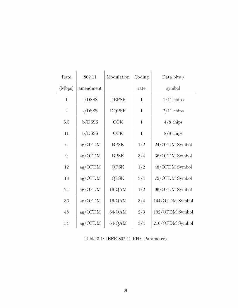
Table 3.1: IEEE 802.11 PHY Parameters.

20

coding schemes and more frequency bands. IEEE 802.11b uses DSSS and adds two

more PHY layer bit rates (5.5 and 11 Mbps). Both IEEE 802.11a and 802.11g

are Orthogonal Frequency-Division Multiplexing systems. We summarize the vari-

ous PHY layer parameters for different variations of the IEEE 802.11 standard in

Table 3.1.

In the following, we briefly describe the OFDM PHYs. More detailed and

complete information can be found in [3]. Each 802.11 frame begins with a PHY

layer header of a format that is known by all WLAN receivers. The PHY layer

header consists of a PLCP (Physical Layer Convergence Procedure) Preamble and a

PLCP Header. The PLCP Preamble contains a number of training symbols, which

help receivers detect signal, configure gain control, align frequency, and synchronize

timing. Time synchronization enables a receiver to determine the boundaries of

each symbol. The PLCP header specifies the modulation and coding scheme and

the length of a frame.

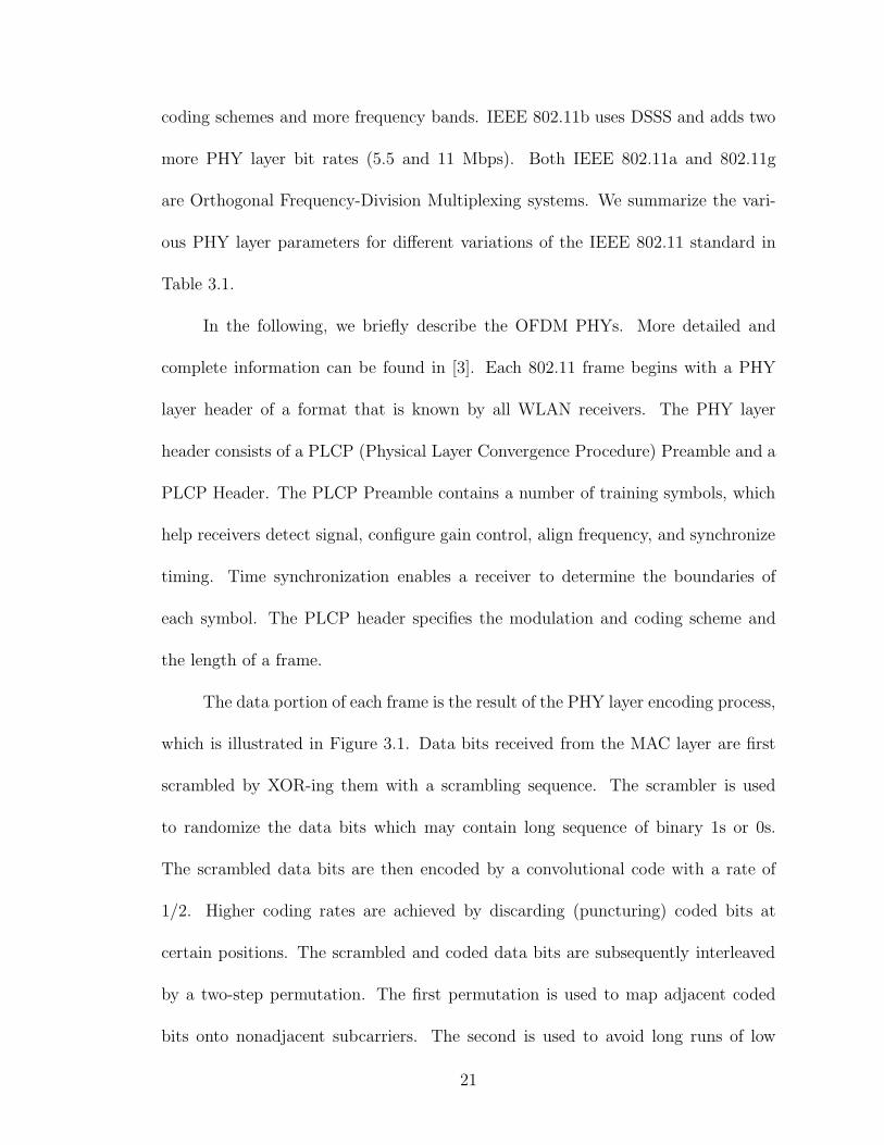
The data portion of each frame is the result of the PHY layer encoding process,

which is illustrated in Figure 3.1. Data bits received from the MAC layer are first

scrambled by XOR-ing them with a scrambling sequence. The scrambler is used

to randomize the data bits which may contain long sequence of binary 1s or 0s.

The scrambled data bits are then encoded by a convolutional code with a rate of

1/2. Higher coding rates are achieved by discarding (puncturing) coded bits at

certain positions. The scrambled and coded data bits are subsequently interleaved

by a two-step permutation. The first permutation is used to map adjacent coded

bits onto nonadjacent subcarriers. The second is used to avoid long runs of low

21

...010010011...

Data bits

...01

10

10

10

1...

Ra

nd

om

bits

R =

1/2

Co

nv

olu

tion

Pu

nc

tua

ting

Inte

rlea

vin

g

Su

b-c

arrie

r

Mo

du

latio

n

Ma

pp

ing

OF

DM

Mo

du

latio

n

Figure 3.1: IEEE 802.11 bit stream encoding process for OFDM modulation.

reliability bits by mapping adjacent coded bits onto less and more significant bits

of a constellation. Finally the scrambled, encoded, and interleaved data bits are

divided into groups with each group converted into a complex number according to

the specified modulation scheme for each sub-carrier of the OFDM system. Every

48 complex numbers are transformed into one clip of time-domain waveform, called

an OFDM symbol, by an Inverse Fast Fourier Transformation (IFFT).

3.3 Experimental Platform

We describe our experimental platform, including the hardware configuration,

RSSI calibration, and experimental procedure.

3.3.1 Hardware Configuration

We use the same hardware platform for both transmitter nodes and receiver

nodes on the primary testbed. Each node is a Soekris Engineering net4826 embed-

ded computer with 2 mini-PCI type III sockets for options such as WLAN cards.

22

We primarily use EMP-8602 and DCMA-82 mini PCI cards in our experiments.

Both use Atheros AR5006 802.11 a/b/g chipsets. On each node the WLAN card is

connected to an omni-directional antenna with 5 dBi (4.8 dBi after cable/connector

loss) gain. We use a USB port on each node to dump the received frames to an

external storage. Each node runs a Debian Linux distribution with kernel version

2.6.15 and its WLAN operation is supported by the MadWifi v0.9.3 device driver.

3.3.2 RSSI Calibration

Most WLAN chipsets report the received signal quality using a numerical value

called the Received Signal Strength Indicator (RSSI) [77, 76]. RSSI is captured

through an analog-to-digital converter on the IF (Intermediate Frequency) level,

and we expect that the relationship between RSSI and dBm to be quasi-linear.

There is, however, not a standard definition for RSSI, leaving device manufacturers

to interpret and implement it differently. We verified that the RSSI reported by

the MadWifi driver for Atheros chipsets is a linear scale representation of the actual

received signal power in dBm using an attenuator-based methodology. We calibrated

the RSSI values of the WLAN cards used in our experiments with the setup shown

in Figure 3.2. In this setup, a step attenuator is placed between the receiver and

the B port of a PE2031 RF signal splitter to produce different power levels of the

received signal.

With this setup, after the attenuation of all individual components is mea-

23

PE

2031TX

RX

Boonton Power Meter

RP-SMA

SMA

L1

L2

L3 L4

LA

LBFreq = 2437 (ch6),

5240 (ch48), 5765 (ch153)

Step Attenuator

Figure 3.2: Calibration setup.

sured, the signal strength at the receiver SRX can be calculated as:

SRX = SPM + L2 + LA − LB − L3 − LS − L4

where Li is cable i’s attenuation, LA and LB are the attenuations of splitter ports

A and B respectively, LS is the attenuation of the step attenuator, and SPM is

the power meter reading. During the calibration process, a WLAN transmitter

periodically transmits data frames of the same length and contents on channel 6

(2.437 GHz). The transmissions are received by both the power meter and the

WLAN receiver. Figure 3.3 shows the screen of the Boonton 4400 RF Peak Power

Meter (http://www.boonton.com), displaying a captured WLAN frame at 54 Mbps

bit rate. The received signal power at the WLAN receiver can then be calculated

and compared with the RSSI value reported by the same WLAN card. The step

attenuator is used to add series of different attenuations before the signal reaches

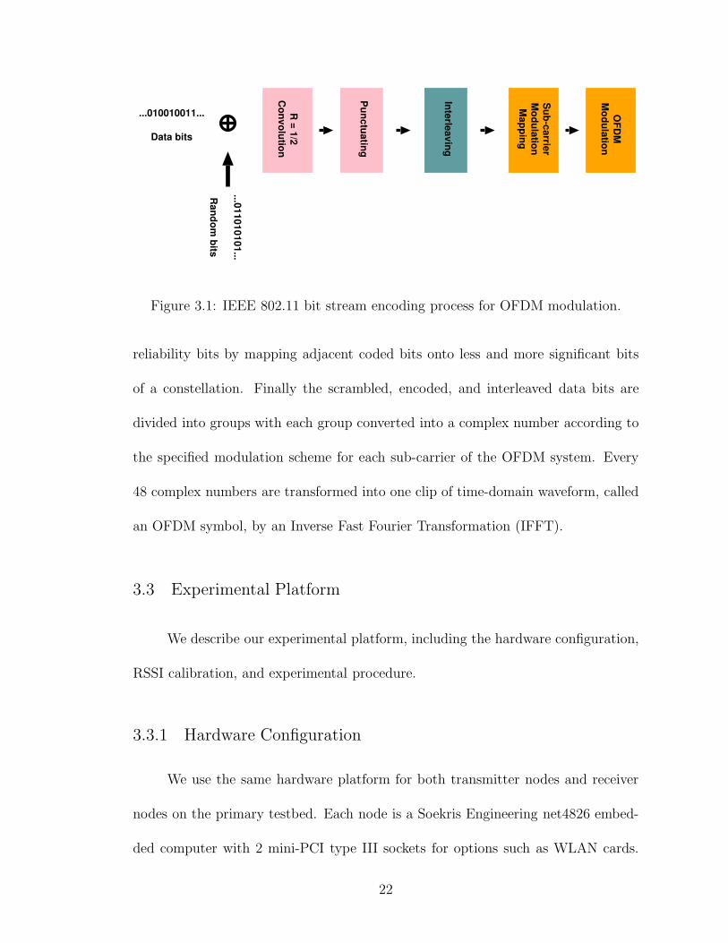
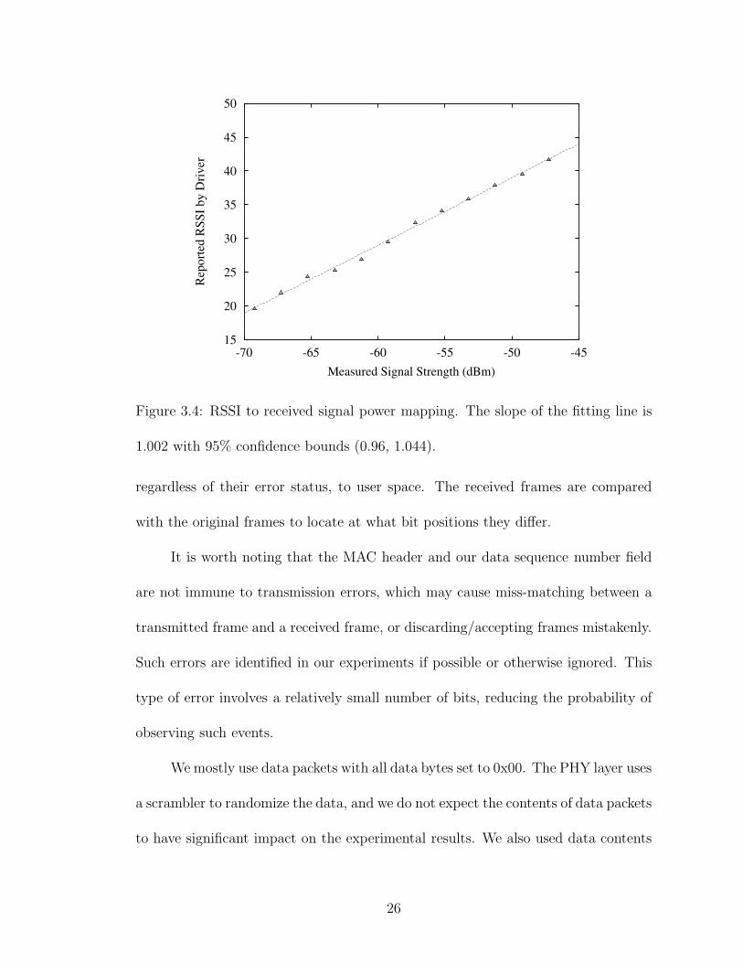
the receiver, as a way of controlling different received signal power. Figure 3.4 plots

a typical calibration result which indicates that for our WLAN cards, RSSI has a

24

Figure 3.3: Boonton 4400 Power Meter Display.

linear relationship with the received signal power in dBm.

3.3.3 Experimental Procedure

During the experiments, we configure one node to be the transmitter and a

number of nodes as the receivers. The EMP-8602 and DCMA-82 cards have two

antenna ports and we connect only one of them to the external antenna. We disable

antenna diversity on both transmitter and receiver nodes to avoid signal quality

variation caused by either end switching to a different antenna port. The transmitter

continuously sends 1024-byte long UDP packets every 10 ms. Within each data

packet, we reserve the first 4 data bytes as a sequence number to match received

frames with originally transmitted frames. We put the receivers under “monitor”

mode and configure them to pass all data frames received from the transmitter,

25

15

20

25

30

35

40

45

50

-70 -65 -60 -55 -50 -45

Rep

ort

ed R

SS

I b

y D

riv

er

Measured Signal Strength (dBm)

Figure 3.4: RSSI to received signal power mapping. The slope of the fitting line is

1.002 with 95% confidence bounds (0.96, 1.044).

regardless of their error status, to user space. The received frames are compared

with the original frames to locate at what bit positions they differ.

It is worth noting that the MAC header and our data sequence number field

are not immune to transmission errors, which may cause miss-matching between a

transmitted frame and a received frame, or discarding/accepting frames mistakenly.

Such errors are identified in our experiments if possible or otherwise ignored. This

type of error involves a relatively small number of bits, reducing the probability of

observing such events.

We mostly use data packets with all data bytes set to 0x00. The PHY layer uses

a scrambler to randomize the data, and we do not expect the contents of data packets

to have significant impact on the experimental results. We also used data contents

26

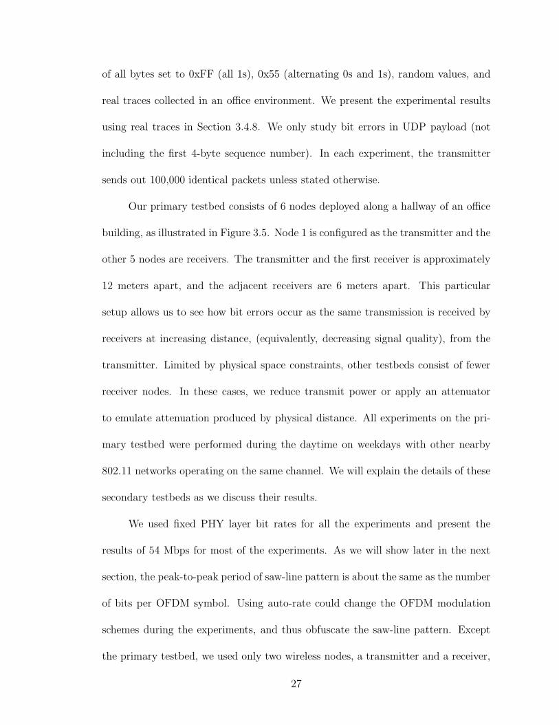
of all bytes set to 0xFF (all 1s), 0x55 (alternating 0s and 1s), random values, and

real traces collected in an office environment. We present the experimental results

using real traces in Section 3.4.8. We only study bit errors in UDP payload (not

including the first 4-byte sequence number). In each experiment, the transmitter

sends out 100,000 identical packets unless stated otherwise.

Our primary testbed consists of 6 nodes deployed along a hallway of an office

building, as illustrated in Figure 3.5. Node 1 is configured as the transmitter and the

other 5 nodes are receivers. The transmitter and the first receiver is approximately

12 meters apart, and the adjacent receivers are 6 meters apart. This particular

setup allows us to see how bit errors occur as the same transmission is received by

receivers at increasing distance, (equivalently, decreasing signal quality), from the

transmitter. Limited by physical space constraints, other testbeds consist of fewer

receiver nodes. In these cases, we reduce transmit power or apply an attenuator

to emulate attenuation produced by physical distance. All experiments on the pri-

mary testbed were performed during the daytime on weekdays with other nearby

802.11 networks operating on the same channel. We will explain the details of these

secondary testbeds as we discuss their results.

We used fixed PHY layer bit rates for all the experiments and present the

results of 54 Mbps for most of the experiments. As we will show later in the next

section, the peak-to-peak period of saw-line pattern is about the same as the number

of bits per OFDM symbol. Using auto-rate could change the OFDM modulation

schemes during the experiments, and thus obfuscate the saw-line pattern. Except

the primary testbed, we used only two wireless nodes, a transmitter and a receiver,

27

14m

48m

1 62 3 4 5

12m 6m

Figure 3.5: Primary testbed topology.

for all other testbeds.

We point out two limitations of our experiments. First, we could only inter-

cept the received bits at the top of the PHY layer (because in commercial WLAN

products the processes in the PHY layer including channel encoding/decoding are

concealed within hardware/firmware, and not accessible from outside). Thus we

cannot measure all of the over-the-air bits, but only those that pass the channel-

decoding procedure. The other is that not all experiments are conducted with the

same transmission power. Transmit power differed on non-primary testbed experi-

ments conducted in small enclosed environments. For these testbeds node distances

were constrained, and we varied transmission power to emulate effects of physical

distance.

28

3.4 Experiments and Results

3.4.1 Overview

In this section, we first present the three bit error patterns, the slope-line,

saw-line and finger patterns, which we identified on the primary testbed. We then

quantitatively model these patterns through curve fitting technology. Finally, we

perform more experiments to exclude some possible reasons of these patterns, such

as environmental effects and hardware platforms. We repeated the experiments

in five other different physical environments, on the Emulab wireless testbed, in a

shielded room, over the cable communications, in mobile and outdoor environments,

to verify that these patterns are not caused by and unique to our primary testbed.

We also repeated the experiments using different hardware platforms and device

drivers, as listed in Table 3.2. The experimental results show that the slope-line

and saw-line patterns are also present on these hardware platforms. However, the

finger pattern exists for only the receivers with Atheros AR5006/AR5212 chipsets.

We have tested not only IEEE 802.11b/g chipsets, but also 802.11n cards. For

most of the experiments, we used the open-source device drivers in Linux operating

systems for various cards. We used the proprietary Linux-based device driver for

the Conexant 3894 mini PCI card with a PRISM chipset and the production-level

Windows-based device driver for the ZyXEL AG-225H USB Adapter with a ZyDAS

ZD1211 chipset.

29

Rec

eive

r

EM

P-8

602

AR

5006

DC

MA

-82

AR

5006

Inte

lP

RO

2100

Bro

adco

mB

CM

4318

Ath

eros

AR

9285

Tra

nsm

itte

rM

adW

ifi/a

th5k

Mad

Wifi

/ath

5kip

w21

00b43

ath9k

EM

P-8

602

AR

5006

∗∗

∗∗

(Mad

Wifi

/ath

5k)

Inte

lP

RO

2915

∗∗

∗∗

(ipw

2200

)

ZyX

EL

ZD

1211

∗

(Win

dow

sdri

ver)

Con

exan

tP

RIS

M∗

∗

(Lin

ux

dri

ver)

Agi

lent

E44

38C

∗

(no

dri

ver)

Bro

adco

mB

CM

4318

∗∗

∗∗

(b43

)

TI

WL12

51∗

∗∗

∗

(wl1

2xx)

Tab

le3.

2:E

xper

imen

tH

ardw

are

Com

bin

atio

ns

(indic

ated

by∗).

30

3.4.2 Bit Error Distribution Patterns

As the received signal quality decreases, the difficulty for a receiver to re-

ceive a frame correctly increases. Loosely speaking, incorrectly-received frames fall

into one of three categories: frames received with bit errors, truncated frames, and

completely-lost frames. Frames with bit errors usually occur when the received sig-

nal quality is marginal. In this case only some bits within a frame are decoded in

error. Although 802.11a/g PHY layer utilizes a convolutional coding scheme for

error corrections, once the number and distribution of erroneous bits exceed the

coding correction capability, the resultant frame after the PHY layer decoding will

contain error bits. Such errors will likely be caught by the integrity check of MAC

layer and cause the frame to be discarded.

During the reception of a frame, if the received signal quality drops so much

that the receiver could no longer even detect the carrier, the PHY layer will prema-

turely exit from frame reception, which results in a truncated frame. In some cases,

a transmitted frame may be completely lost. Various conditions can cause entire

frames to be lost. For instance, the receiver may not detect the carrier at all, or it

may not be able to lock its clock with the synchronization symbols included in the

beginning of the frame, or it may not receive and/or decode the PLCP preamble

and PLCP header of the frame.

We have identified a number of unexpected bit error probability patterns from

the primary testbed measurements. Figure 3.6 is a histogram of where the erroneous

bits are located for receiver node 3 on the primary testbed. The x-axis is the bit

31

0

0.02

0.04

0.06

0.08

0.1

0 1000 2000 3000 4000 5000 6000 7000 8000 9000

Fre

q.

of

Bit

Err

ors

(n

orm

aliz

ed)

Bit Position of Error

txpower = 6dBm rate = 54M

slope

Node 3 @ Position 3

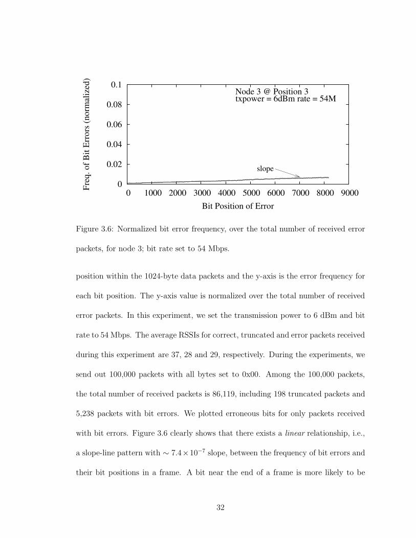
Figure 3.6: Normalized bit error frequency, over the total number of received error

packets, for node 3; bit rate set to 54 Mbps.

position within the 1024-byte data packets and the y-axis is the error frequency for

each bit position. The y-axis value is normalized over the total number of received

error packets. In this experiment, we set the transmission power to 6 dBm and bit

rate to 54 Mbps. The average RSSIs for correct, truncated and error packets received

during this experiment are 37, 28 and 29, respectively. During the experiments, we

send out 100,000 packets with all bytes set to 0x00. Among the 100,000 packets,

the total number of received packets is 86,119, including 198 truncated packets and

5,238 packets with bit errors. We plotted erroneous bits for only packets received

with bit errors. Figure 3.6 clearly shows that there exists a linear relationship, i.e.,

a slope-line pattern with ∼ 7.4×10−7 slope, between the frequency of bit errors and

their bit positions in a frame. A bit near the end of a frame is more likely to be

32

0

0.02

0.04

0.06

0.08

0.1

0 1000 2000 3000 4000 5000 6000 7000 8000 9000

Fre

q.

of

Bit

Err

ors

(n

orm

aliz

ed)



216b

saw-line

finger

Node 4 @ Position 4

Figure 3.7: Normalized bit error frequency for node 4 with bit rate 54 Mbps. The

average RSSIs of correct packets, truncated packets and packets with bit errors are

36, 21 and 22, respectively.

received in error than a bit near the beginning of the frame. For example, a bit at

position 8,000 (0.00656) is about 3 times more likely to be received in error than a

bit at position 1,000 (0.00161).

We show the same bit error frequency vs. bit position plot with the data

collected on receiver node 4, which is farther away from the transmitter than node

3, during the same experiment in Figure 3.7. This plot exhibits different bit error

behavior. While the slope pattern is still present, Figure 3.7 also displays two

additional patterns: what we refer to as the saw-line pattern and the finger pattern.

The saw-line pattern is the fine zig-zag line that goes across the full length of the

frame. What is interesting about this pattern is that the saw-tooth peak-to-peak

33

0

0.02

0.04

0.06

0.08

0.1

0 1000 2000 3000 4000 5000 6000 7000 8000 9000

Fre

q.

of

Bit

Err

ors

(n

orm

aliz

ed)



144b

Node 4 @ Position 4




period is about the same as the number of bits each OFDM symbol carries at

54 Mbps bit rate. The finger pattern refers to the larger peaks, which begins to

appear after certain bit position (around the 2,000th bit) and repeats at a fairly

regular interval. The overall plot of bit error frequencies in Figure 3.7 is actually

the superposition of all three patterns.

We also observed similar patterns from the results obtained from nodes 5 and

6. Node 2 is the closest to the transmitter among all receivers. It has the best

received signal quality. We were not able to collect enough frames with erroneous

bits to produce any meaningful bit error histogram plots for node 2.

We repeated the experiments with bit rates set to 36 and 48 Mbps, and with

34

0

0.02

0.04

0.06

0.08

0.1

0 1000 2000 3000 4000 5000 6000 7000 8000 9000

Fre

q.

of

Bit

Err

ors

(n

orm

aliz

ed)



192b

Node 4 @ Position 4




different data contents (all bytes set to 0xFF, 0x55, or random value). Due to space

limitation, we only show the plots for 36 and 48 Mbps with all bytes set to 0x00 in

Figure 3.8 and Figure 3.9. While we can observe the same three patterns from all

these plots, including those with 0xFF, 0x55 and random UDP payload, the peak-

to-peak period of saw-line pattern changes for different OFDM bit rates (144 bits

for 36 Mbps and 192 bits for 48 Mbps).

3.4.3 Quantification of Patterns

In this subsection, we further analyze the three patterns identified above by

quantitatively modeling the patterns using curve fitting techniques.

35

As we mentioned above, the bit error patterns are apparently a superposition

of slope-line, saw-line and fingers. We first use a linear function l(x) = u ∗ x + v to

fit the slope-line pattern. Because the fingers have high peaks that would affect the

fitting result, we calculate the slope parameters using a modified plot by removing

all the data points in the finger regions. We then model the saw-line for the first

2,000 bits, because the fingers only appear after certain point and within the first

2,000 bits there is no finger. Given the periodic nature of saw-line pattern, we use

the most common periodic curve fitting function to model it:

s(x) = a + b ∗ cos(ω ∗ x) + c ∗ sin(ω ∗ x) + l(x)

where l(x) is the bit errors contributed by the slope line at position x.

We summarize the fitting results for the patterns observed at node 4 for 54

Mbps (Figure 3.7), 48 Mbps (Figure 3.9), and 36 Mbps (Figure 3.8) in Table 3.3.

For the saw-line fitting, after we determine the value of ω, we can calculate the

saw-tooth period as 2 ∗ π/ω, which is shown in the last column of Table 3.3. The

calculated saw-tooth periods have verified our earlier observation that the saw-line

period is exactly the symbol length for the corresponding bit rate (216 for 54 Mbps,

192 for 48 Mbps and 144 for 36 Mbps).

Once the bit errors contributed by the slope and saw-line patterns are deter-

mined, they can be removed and all remaining bit errors are considered to be the

result of finger pattern. We present the width of the 6 fingers found in the results

for node 4 from all experiments in Table 3.4. The numbers in the parentheses are

the ratio between the finger width and the corresponding symbol length. This table

36

Bit Rate u v ω at 95% confidence Period

54M 5.1 × 10−7 7.3 × 10−3 (0.02906, 0.02917) 215.8

48M 4.5 × 10−7 8.8 × 10−3 (0.0325, 0.033) 191.9

36M 6.8 × 10−7 1.1 × 10−2 (0.04354, 0.04372) 144.0

Table 3.3: The slopes and intercepts of the fitting lines, and the calculated periods

of the fitting saw-lines.

Bit Rate 54M 48M 36M

Finger 1 648(3x) 775(4.036x) 436(3.028x)

Finger 2 858(3.972x) 768(4x) 436(3.028x)

Finger 3 848(4x) 768(4x) 432(3x)

Finger 4 648(3x) 768(4x) 432(3x)

Finger 5 649(3.005x) 768(4.x) 576(4x)

Finger 6 835(3.87x) 761(3.964x) 576(4x)

Table 3.4: Finger Width.

shows that the widths of the fingers are multiples of the corresponding number of

data bits per OFDM symbol. We curve fit the bit error patterns identified on other

testbeds; we present results from these testbeds and their curve fits next.

3.4.4 Different Physical Environments

We have repeated our experiments in five other different environments (Em-

ulab wireless testbed, a shielded room, over the cable communications, mobile and

37

outdoor environments) to verify that the three identified patterns are not the result

of the specific environment of our primary testbed. We present the experimental

results of the last two challenged mobile and outdoor environments in Section 3.4.7.

3.4.4.1 Emulab Wireless Testbed

Although Emulab is often used to provide emulated network environments for

experiments of wired networks, the Emulab wireless testbed uses over-the-air com-

munication through IEEE 802.11 wireless interfaces between stationary PC nodes

scattered around a typical office building. Each Emulab node has two Netgear

WAG311 cards, which use Atheros AR5212 802.11a/b/g chipsets. Figure 3.10 shows

the result when node pcwf2 is selected as the transmitter and pcwf 13 is used as the

receiver,1 which verifies the three bit error patterns. We note that in this experi-

ment, not only the environment is different, the hardware platform is also different

(Atheros AR5212 vs. Atheros AR5006).

3.4.4.2 Shielded Room

Our own testbed and Emulab wireless testbed are all deployed in office build-

ings. To identify whether these patterns are caused by radio interference in the

experimental environment, we construct another testbed using the same nodes as in

the primary testbed in a small shielded room located in the AT&T Shannon Lab.

The shielded room is a 12’ x 12’ room with metal floor, ceiling, and walls. It is

1The floorplan of Emulab wireless testbed is available at https://www.emulab.net/floormap.

php3.

38

0

0.05

0.1

0.15

0.2

0.25

0.3

0 1000 2000 3000 4000 5000 6000 7000 8000 9000

Fre

q. of

Bit

Err

ors

(norm

aliz

ed)


txpower = 7dBm rate = 54MNode pcwf13 @ Emulab

Figure 3.10: Normalized bit error frequency for node pcwf13 of Emulab testbed.

Node pcwf2 is selected as the transmitter. The slope of the fitting line is 2.553×10−6

with 95% confidence bounds (2.354×10−6, 2.751×10−6) and the saw-tooth period

is 215.917 with 95% confidence bounds (215.473, 216.438).

0

0.02

0.04

0.06

0.08

0.1

0 1000 2000 3000 4000 5000 6000 7000 8000 9000

Fre

q. of

Bit

Err

ors

(norm

aliz

ed)


txpower = 6dBm rate = 54MNode 3 @ Shielded Room

Figure 3.11: Normalized bit error frequency for node 3 in a shielded room. The

slope of the fitting line is 1.478× 10−6 with 95% confidence bounds (1.387× 10−6,

1.571 × 10−6) and the saw-tooth period is 216.886 with 95% confidence bounds

(215.695, 218.166).

39

designed to shield what is in the room from all external radio interferences. The

transmitter is located in one corner of the room and the receiver is put in another

corner diagonally across the room. We present the result for node 3 in Figure 3.11.

The bit rate is 54 Mbps. The total number of packets transmitted is 10,000. The

three aforementioned bit error patterns are still easy to observe.

3.4.4.3 Cable

Although the shielded room can separate external interferences, it cannot pre-

vent all environmental effects on over-the-air wireless transmissions. One particular

example is reflection. Hence we conducted another group of experiments in a lab-

oratory where the transmitter and receiver are directly connected using the same

setup as we used for RSSI calibration (Figure 3.2). The step attenuator is used to

gradually reduce the received signal strength. In this group of experiments, the bit

rate is 54 Mbps and 10,000 packets are transmitted over the directly connected sys-

tem. Because there is little fluctuation in the received signal quality in this case, the

transition from very good reception (almost no packets received with bit errors) to

very poor (almost no packets received correctly) is very rapid. Figure 3.12 captures

the bit error frequency when the average RSSI for the packets with bit errors is only

19. Still, the three patterns are identifiable.

Another interesting finding is that there is no truncated packet received when

the transmissions are over the cables. This indicates that frame truncations are

not likely due to transmitter and receiver hardware issues but likely because of

40

0

0.02

0.04

0.06

0.08

0.1

0.12

0.14

0 1000 2000 3000 4000 5000 6000 7000 8000 9000

Fre

q.

of

Bit

Err

ors

(n

orm

aliz

ed)


txpower = 6dBm rate = 54MConnected via Cables

Figure 3.12: Normalized bit error frequency for over the cable communication. The

slope of the fitting line is 4.720 × 10−7 with 95% confidence bounds (3.849 × 10−7,


(216.066, 216.961).

fluctuations of wireless channel conditions and interferences.

3.4.5 Different Hardware Platforms

The experimental results presented so far were all obtained using WLAN cards

made of Atheros AR5006/AR5212 chipsets. This raises another question: do these

patterns only occur on specific hardware platforms? In this subsection we present

experimental results obtained using hardware made by different manufactures with

different chipsets.

A problem of using WLAN hardware with non-Atheros chipsets is that the

device drivers for those chipsets normally support only a very limited configuration

interface. We need to control the bit rate and transmit power for each transmitter

41

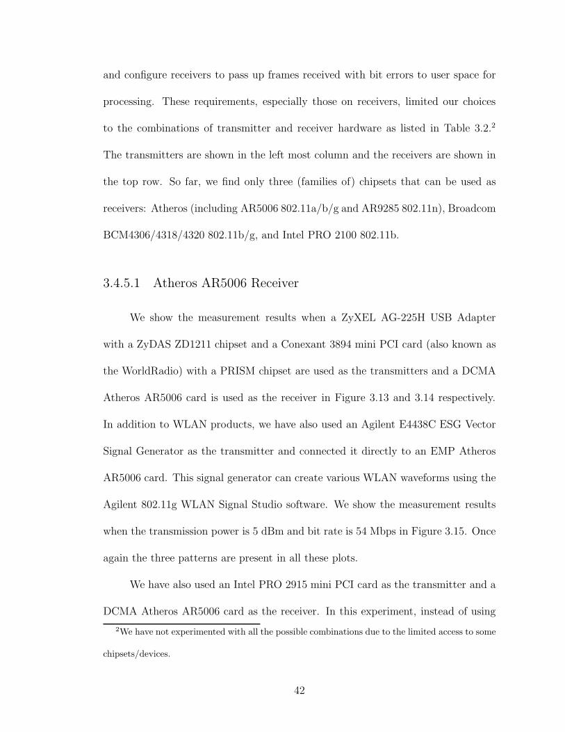
and configure receivers to pass up frames received with bit errors to user space for

processing. These requirements, especially those on receivers, limited our choices

to the combinations of transmitter and receiver hardware as listed in Table 3.2.2

The transmitters are shown in the left most column and the receivers are shown in

the top row. So far, we find only three (families of) chipsets that can be used as

receivers: Atheros (including AR5006 802.11a/b/g and AR9285 802.11n), Broadcom

BCM4306/4318/4320 802.11b/g, and Intel PRO 2100 802.11b.

3.4.5.1 Atheros AR5006 Receiver

We show the measurement results when a ZyXEL AG-225H USB Adapter

with a ZyDAS ZD1211 chipset and a Conexant 3894 mini PCI card (also known as

the WorldRadio) with a PRISM chipset are used as the transmitters and a DCMA

Atheros AR5006 card is used as the receiver in Figure 3.13 and 3.14 respectively.

In addition to WLAN products, we have also used an Agilent E4438C ESG Vector

Signal Generator as the transmitter and connected it directly to an EMP Atheros

AR5006 card. This signal generator can create various WLAN waveforms using the

Agilent 802.11g WLAN Signal Studio software. We show the measurement results

when the transmission power is 5 dBm and bit rate is 54 Mbps in Figure 3.15. Once

again the three patterns are present in all these plots.

We have also used an Intel PRO 2915 mini PCI card as the transmitter and a

DCMA Atheros AR5006 card as the receiver. In this experiment, instead of using

2We have not experimented with all the possible combinations due to the limited access to some

chipsets/devices.

42

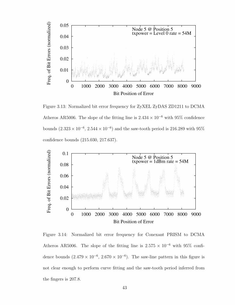
0

0.01

0.02

0.03

0.04

0.05

0 1000 2000 3000 4000 5000 6000 7000 8000 9000

Fre

q. of

Bit

Err

ors

(norm

aliz

ed)


txpower = Level 0 rate = 54MNode 5 @ Position 5

Figure 3.13: Normalized bit error frequency for ZyXEL ZyDAS ZD1211 to DCMA

Atheros AR5006. The slope of the fitting line is 2.434× 10−6 with 95% confidence

bounds (2.323× 10−6, 2.544× 10−6) and the saw-tooth period is 216.289 with 95%

confidence bounds (215.030, 217.637).

0

0.02

0.04

0.06

0.08

0.1

0 1000 2000 3000 4000 5000 6000 7000 8000 9000

Fre

q. of

Bit

Err

ors

(norm

aliz

ed)


txpower = 1dBm rate = 54MNode 5 @ Position 5

Figure 3.14: Normalized bit error frequency for Conexant PRISM to DCMA

Atheros AR5006. The slope of the fitting line is 2.575 × 10−6 with 95% confi-

dence bounds (2.479 × 10−6, 2.670 × 10−6). The saw-line pattern in this figure is

not clear enough to perform curve fitting and the saw-tooth period inferred from

the fingers is 207.8.

43

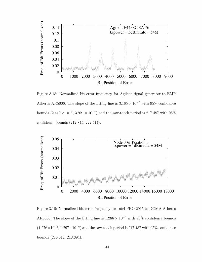
0

0.02

0.04

0.06

0.08

0.1

0.12

0.14

0 1000 2000 3000 4000 5000 6000 7000 8000 9000

Fre

q. of

Bit

Err

ors

(norm

aliz

ed)


txpower = 5dBm rate = 54MAgilent E4438C SA 76

Figure 3.15: Normalized bit error frequency for Agilent signal generator to EMP

Atheros AR5006. The slope of the fitting line is 3.165× 10−7 with 95% confidence



0

0.01

0.02

0.03

0.04

0.05

0 2000 4000 6000 8000 10000 12000 14000 16000 18000

Fre

q. of

Bit

Err

ors

(norm

aliz

ed)



Figure 3.16: Normalized bit error frequency for Intel PRO 2915 to DCMA Atheros

AR5006. The slope of the fitting line is 1.286 × 10−6 with 95% confidence bounds

(1.276×10−6, 1.297×10−6) and the saw-tooth period is 217.487 with 95% confidence

bounds (216.512, 218.394).

44

1024-byte packets we used 2200-byte packets to see if the patterns continue as the

packet length. The result, as plotted in Figure 3.16, shows that all three patterns

continue all the way till the end of the frames, regardless of the frame length. An-

other interesting characteristic of this plot is that the fingers are “flipped”. Instead

of being regions with elevated bit error probability, the fingers here are actually

regions with reduced bit error probability.

3.4.5.2 Broadcom Receiver

Benefiting from OpenFWWF [35], an open source firmware for Broadcom WiFi

cards, we can also modify the firmware to make the BCM4318 chipsets pass the cor-

rupted frames to user space. We show the experimental results when Broadcom

BCM4318, EMP Atheros AR5006, and Intel PRO 2195 cards are used as transmit-

ters in Figure 3.17, 3.18 and 3.19, respectively. Interestingly, when a Broadcom

BCM4318 card is used as the receiver, we do not observe the finger pattern for these

three transmitters. For the Broadcom BCM4318 transmitter, although the saw-line

is not regular and some saw-teeth have higher peaks, compared to the other two

transmitters, we cannot consider these saw-teeth as fingers, because the widths of

fingers are multiples (either 3 or 4, as in Table 3.4) of those of saw-teeth. However,

the slope and saw-line patterns are still evident in these three figures.

45

0

0.02

0.04

0.06

0.08

0.1

0.12

0.14

0 1000 2000 3000 4000 5000 6000 7000 8000 9000

Fre

q. of

Bit

Err

ors

(norm

aliz

ed)


txpower = 5dBm rate = 54MBCM4318@UMD

Figure 3.17: Normalized bit error frequency for Broadcom BCM4318 to Broadcom

BCM4318. The slope of the fitting line is 6.506×10−6 with 95% confidence bounds


bounds (215.917, 216.140).

0

0.05

0.1

0.15

0.2

0 1000 2000 3000 4000 5000 6000 7000 8000 9000

Fre

q. of

Bit

Err

ors

(norm

aliz

ed)


txpower = 4dBm rate = 54MBCM4318@UMD

Figure 3.18: Normalized bit error frequency for EMP Atheros AR5006 to Broadcom



bounds (215.769, 215.917).

46

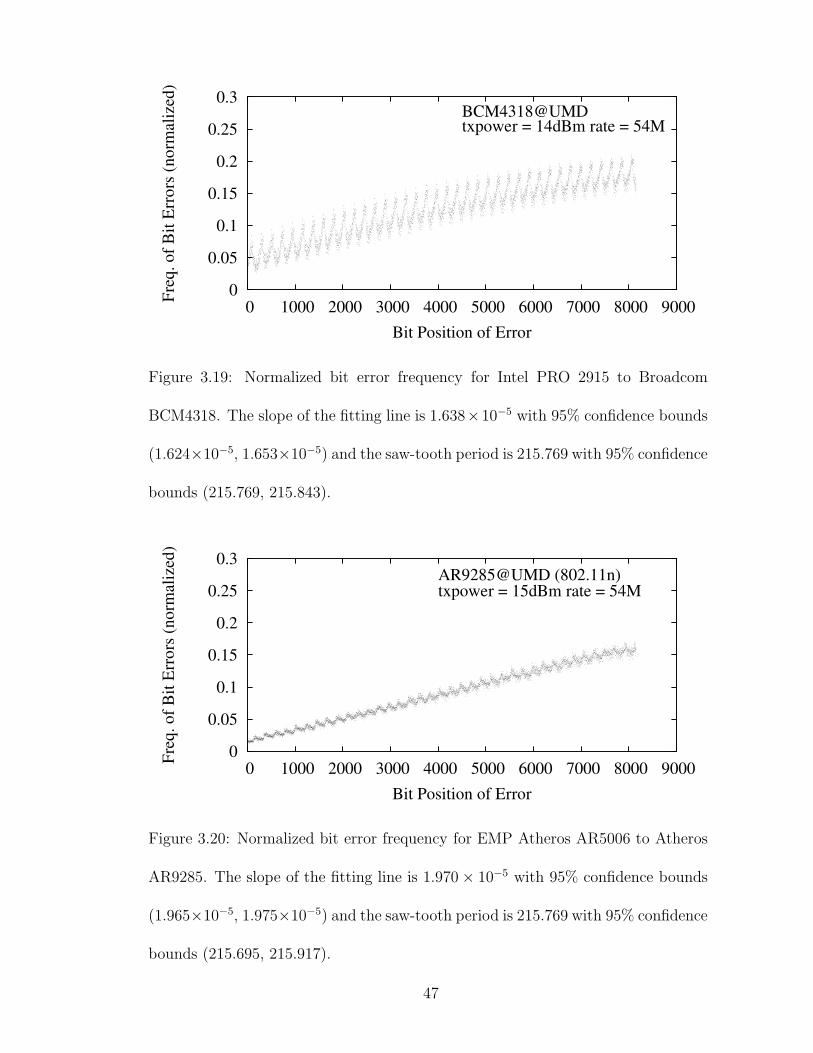
0

0.05

0.1

0.15

0.2

0.25

0.3

0 1000 2000 3000 4000 5000 6000 7000 8000 9000

Fre

q. of

Bit

Err

ors

(norm

aliz

ed)


BCM4318@UMDtxpower = 14dBm rate = 54M

Figure 3.19: Normalized bit error frequency for Intel PRO 2915 to Broadcom



bounds (215.769, 215.843).

0

0.05

0.1

0.15

0.2

0.25

0.3

0 1000 2000 3000 4000 5000 6000 7000 8000 9000

Fre

q. of

Bit

Err

ors

(norm

aliz

ed)


AR9285@UMD (802.11n)txpower = 15dBm rate = 54M

Figure 3.20: Normalized bit error frequency for EMP Atheros AR5006 to Atheros



bounds (215.695, 215.917).

47

3.4.5.3 Atheros AR9285 Receiver

Leveraging the recently developed iw utility for wireless devices, we can easily

add a monitor interface on Atheros AR9285 802.11n cards that can pass error packets

to user space. We show the experimental results when EMP Atheros AR5006, Intel

PRO 2195, and Broadcom BCM4318 cards are used as transmitters in Figure 3.20,

3.21 and 3.22, respectively. Similar to the results when a Broadcom BCM4318

card is used as the receiver, we do not observe the finger pattern for these three

transmitters with an Atheros AR9285 card as the receiver, although the slope-line

and saw-line patterns still exist.

Remark: Similar finger patterns were also observed in prior work, such as from

an 802.11b testbed using Harris/Intersil PRISM I chipsets in an industrial environ-

ment [88], an in-building 802.11a testbed with Atheros 5212 chipsets [62], and a

testbed of a static AP and a mobile user [60]. However, all of these testbeds used

the old version of 802.11 chipsets (e.g., PRISM I, or Atheros 5212). We verified that

the finger pattern does not appear when Broadcom BCM4318 and Atheros AR9285

802.11n chipsets (a newer product of Atheros) are used as the receivers.

3.4.5.4 Intel Receiver

Intel PRO 2100 chipsets support only 802.11b mode which uses DSSS modu-

lation. Thus, we present the experimental results using the Intel PRO 2100 receiver

in the next subsection (Figure 3.24).

48

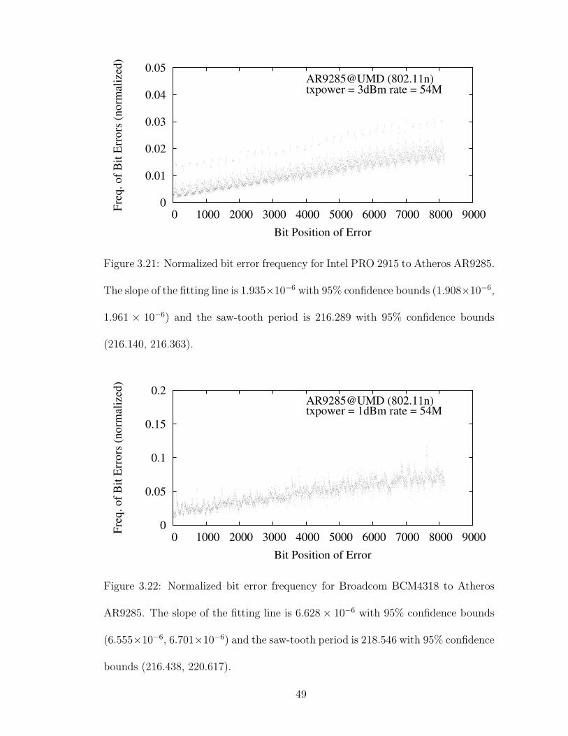
0

0.01

0.02

0.03

0.04

0.05

0 1000 2000 3000 4000 5000 6000 7000 8000 9000

Fre

q. of

Bit

Err

ors

(norm

aliz

ed)



Figure 3.21: Normalized bit error frequency for Intel PRO 2915 to Atheros AR9285.

The slope of the fitting line is 1.935×10−6 with 95% confidence bounds (1.908×10−6,


(216.140, 216.363).

0

0.05

0.1

0.15

0.2

0 1000 2000 3000 4000 5000 6000 7000 8000 9000

Fre

q. of

Bit

Err

ors

(norm

aliz

ed)



Figure 3.22: Normalized bit error frequency for Broadcom BCM4318 to Atheros



bounds (216.438, 220.617).

49

3.4.6 Different Modulation

IEEE 802.11b uses DSSS CCK modulation which is quite different from the

OFDM modulation used by IEEE 802.11a/g. Intrigued by the fact that the saw-

tooth peak period is exactly at symbol length, we repeated the experiments on the

primary testbed with 802.11b settings (e.g., 11 Mbps bit rate). We show the result in

Figure 3.23. The slope and saw-line patterns are observable in this figure. However,

instead of being the number of bits each symbol carries, the saw-line peak-to-peak

distance is much larger (e.g., 9 symbol lengths in Figure 3.23). Finally, Figure 3.24

shows the result when a Conexant PRISM card is used as the transmitter and an

Intel PRO 2100 card is configured as the receiver. The bit rate is 11Mbps, the

maximal rate for IEEE 802.11b which is the only mode supported by Intel PRO

2100. Under this configuration, we can still find the slope.

3.4.7 Challenged 802.11 Environments

With the increasing popularity of WiFi-enabled smartphones, IEEE 802.11

technology has been widely used for more challenged environments (compared to

traditional indoor WLANs), including mobile and outdoor environments. We also

performed experiments for these two challenged environments using smartphones.

We used a Nokia N900 smartphone as the transmitter for these experiments. Its

default OS, Maemo 5, is an open source Linux distribution (2.6.28 kernel). The WiFi

chipset is Texas Instruments WL1251, which supports 802.11b/g. The receiver was

an Asus Eee PC netbook equipped with an Atheros AR9285 802.11n card.

50

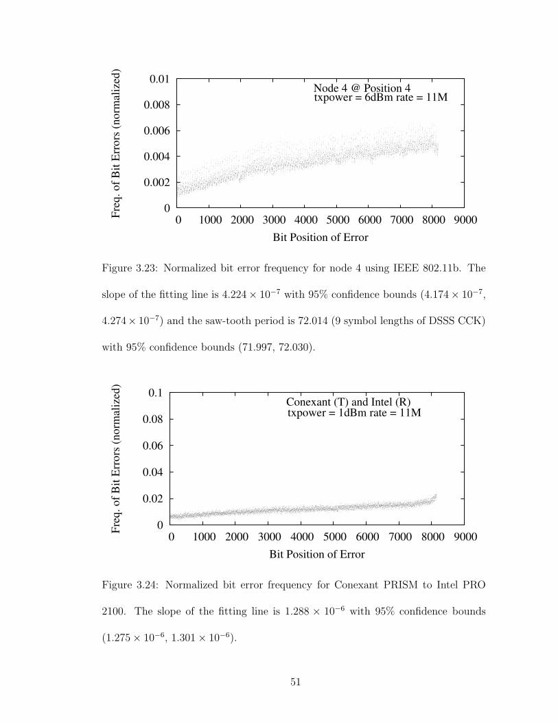
0

0.002

0.004

0.006

0.008

0.01

0 1000 2000 3000 4000 5000 6000 7000 8000 9000

Fre

q. of

Bit

Err

ors

(norm

aliz

ed)



Figure 3.23: Normalized bit error frequency for node 4 using IEEE 802.11b. The

slope of the fitting line is 4.224× 10−7 with 95% confidence bounds (4.174× 10−7,

4.274× 10−7) and the saw-tooth period is 72.014 (9 symbol lengths of DSSS CCK)

with 95% confidence bounds (71.997, 72.030).

0

0.02

0.04

0.06

0.08

0.1

0 1000 2000 3000 4000 5000 6000 7000 8000 9000

Fre

q. of

Bit

Err

ors

(norm

aliz

ed)


txpower = 1dBm rate = 11MConexant (T) and Intel (R)

Figure 3.24: Normalized bit error frequency for Conexant PRISM to Intel PRO

2100. The slope of the fitting line is 1.288 × 10−6 with 95% confidence bounds

(1.275 × 10−6, 1.301 × 10−6).

51

ReceiverA B

40m 9m

Figure 3.25: The mobile testbed in a hallway. During the experiments, we walk

between A and B with the smartphone transmitter in hand.

During the mobile experiments, we set up the receiver (which is also the moni-

tor to dump error packets) in a hallway of an office building, as shown in Figure. 3.25.

Then we walked between two locations, A and B in Figure. 3.25, in the same hallway

with the smartphone transmitter in hand. We performed the outdoor experiments

in an empty parking lot in the University of Maryland during a weekend. For both

environments, we collected error packets transmitted at 54 Mbps.

We show the result for mobile environment in Figure 3.26 and outdoor envi-

ronment in Figure 3.27, respectively. As we can see from these two figures, the slope

and saw-line patterns are still present for these challenged environments. However,

we do not identify a clear finger pattern, which further verifies the experimental

results in Section 3.4.5. To figure out whether the finger pattern appears in these

environments, we repeated the mobile experiments with a dedicated monitor using a

DCMA Atheros AR5006 card. We plot the result in Figure 3.28, which again shows

a superposition of the three patterns. Note that the monitor was supported by the

ath5k device driver for Atheros chipsets, which is a replacement of the MadWifi

device driver that we have used for all the previous experiments, where Atheros

52

0

0.02

0.04

0.06

0.08

0.1

0 1000 2000 3000 4000 5000 6000 7000 8000 9000

Fre

q. of

Bit

Err

ors

(norm

aliz

ed)



Figure 3.26: Normalized bit error frequency for TI WL1251 to Atheros AR9285,

mobile environment. The slope of the fitting line is 3.925×10−6 with 95% confidence



0

0.05

0.1

0.15

0.2

0.25

0.3

0 1000 2000 3000 4000 5000 6000 7000 8000 9000

Fre

q. of

Bit

Err

ors

(norm

aliz

ed)



Figure 3.27: Normalized bit error frequency for TI WL1251 to Atheros AR9285,

outdoor environment. The slope of the fitting line is 4.676 × 10−6 with 95% con-

fidence bounds (4.551 × 10−6, 4.801 × 10−6) and the saw-tooth period is 215.917


53

AR5006 and AR5212 chipsets were involved.

3.4.8 Real Traces

We finally performed experiments to study bit error patterns using traces

collected in an office environment, although we are confident that the identified bit

error patterns are not caused by packet contents.

We collected real IEEE 802.11 traces over-the-air in an office building which

contain only data packets with captured length at least 1200 bytes. Then we fed the

traces to a tool, called Bits-Analyzer, which works as follows. At the beginning of a

single experiment, the transmitter retrieves a packet from the traces, sends it to the

receiver through an Ethernet control channel, and then repeatedly transmits 1024

bytes of its payload over the wireless channel. When the receiver gets a corrupted

packet, it compares the received data bits with those in the reference packet received

through the control channel to determine which bits are corrupted. After the receiver

gets enough number of error receptions of a data packet (10 in our experiments) on

its monitor mode 802.11 interface, it notifies the transmitter to move on to the next

packet in the traces.

We present the experimental results using the EMP Atheros AR5006 trans-

mitter and the DCMA Atheros AR5006 receiver in Figure 3.29. The real trace

contains 10,000 data packets. As we can see from this figure, these three patterns

are independent of packet payloads and still exist when an Atheros AR5006 chipset

is used as a receiver.

54

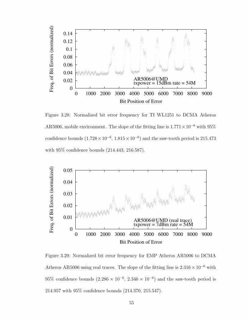
0

0.02

0.04

0.06

0.08

0.1

0.12

0.14

0 1000 2000 3000 4000 5000 6000 7000 8000 9000

Fre

q. of

Bit

Err

ors

(norm

aliz

ed)


AR5006@UMDtxpower = 15dBm rate = 54M

Figure 3.28: Normalized bit error frequency for TI WL1251 to DCMA Atheros

AR5006, mobile environment. The slope of the fitting line is 1.771×10−6 with 95%

confidence bounds (1.728×10−6, 1.815×10−6) and the saw-tooth period is 215.473


0

0.01

0.02

0.03

0.04

0.05

0 1000 2000 3000 4000 5000 6000 7000 8000 9000

Fre

q. of

Bit

Err

ors

(norm

aliz

ed)


AR5006@UMD (real trace)txpower = 7dBm rate = 54M

Figure 3.29: Normalized bit error frequency for EMP Atheros AR5006 to DCMA

Atheros AR5006 using real traces. The slope of the fitting line is 2.316×10−6 with

95% confidence bounds (2.286 × 10−6, 2.346 × 10−6) and the saw-tooth period is

214.957 with 95% confidence bounds (214.370, 215.547).

55

3.4.9 Summary

During the measurement study on IEEE 802.11 WLAN testbeds, we have

identified three distinct patterns for bit error probabilities with respect to bit posi-

tions: slope-line, saw-line, and finger. We have verified that the presence of the first

two patterns is consistent in different environments and across different hardware

platforms.

In our experience, the slope pattern is universal. It is present in all exper-

imental results. This pattern shows that there is apparently a linear relationship

between the chance of bit error occurrence and its bit position. Bits near the end

of a frame are more likely to be received in error compared to bits in earlier portion

of a frame.

The slope-line pattern may appear alone. However, as signal quality drops

further, the other two patterns begin to show. For example, we can see only the

slope pattern in Figure 3.6 for receiver node 3, but all three patterns in Figure 3.7

for receiver node 4. As node 4 is further away from the transmitter, compared to

node 3 (as shown in Figure 3.5), the quality of the received signal at node 4 may

be worse than that at node 3 for the same transmitted packet. The saw-line is also

observable in almost all experimental results. For OFDM transmissions, the saw-

tooth peak-to-peak distance is exactly the number of bits carried by each OFDM

symbol. For DSSS transmissions, the peak-to-peak distance appears to be a multiple

of the number of bits carried by each symbol.

The finger pattern has been observed mainly in OFDM transmissions, but not

56

for all hardware platforms. So far, we have not identified clear finger patterns for

the Broadcom BCM4318 and Atheros AR9285 receivers. It may be either in the

form of “peaks” or “valleys”. The width of the fingers is a multiple of the number

of bits carried by each symbol, usually 3-4 symbols.

3.5 Hypotheses and Discussions

It is difficult to pinpoint the exact causes of the identified patterns without

access to detailed WLAN hardware design. We explore some possible reasons for

the slope-line, saw-line, and finger patterns in this section. We note that these

patterns are not likely to be caused by flaws/bugs in device drivers, because we

used 9 different drivers on 10 different platforms in our experiments.

Two apparent reasons for the slope-line pattern are clock drift and changes

of channel conditions. As mentioned before, synchronization between receiver and

transmitter clocks is done only through receiving special symbols prepended at the

very beginning of each frame. Although there are four pilot subcarriers in each

OFDM symbol in order to make the coherent detection robust against phase noise

and frequency offsets [3], and thus make a receiver be able to track clock drifts

and channel errors, commodity hardware may do a poor job in implementing these

pilot subcarriers, probably due to cost reasons. Thus, because of synchronization

errors and clock drifting, as time goes on and bit reception progresses, the offset be-

tween the receiver’s clock and transmitter’s clock increases. As a result, boundary

alignment of transmitted symbols and receiver samples deteriorates. This inevitably

57

leads to increased bit error probability. Moreover, transmitters only sense the wire-

less channel prior to transmission. Therefore, some hidden terminals may start their

own transmissions during a packet reception, which will generate external interfer-

ences. Although this is more likely to cause truncated frames, we cannot rule out

this being a reason for later positions having higher bit error probability than earlier

positions.

The saw-line pattern of OFDM transmissions is likely caused by the frequency

selectivity characteristic of wireless channel, the transmitter, and the receiver [83].

Because of this frequency selectivity, certain OFDM subcarriers may experience

higher error rates than others [37]. The interleaver of 802.11a/g is designed to map

adjacent data bits to subcarriers that are far apart from each other. However, be-

cause the interleaving permutation is identical for all symbols, frequency selectivity

induced bit error pattern will also be repeated for every symbol. This is the reason

that the saw-line peak-to-peak distance is exactly the OFDM symbol length. By

exploring the difference between the error rates of these subcarriers, we may be able

to design more efficient retransmission protocols. For example, Li et al. [52] recently

propose Remap, a scheme that permutes the bit-to-subcarrier mapping after each

retransmission and thus improve decoding efficiency and link throughput.

Another possible reason for the saw-line pattern is the residual Sampling Fre-

quency Offset (SFO), which is caused by small oscillator frequency differences be-

tween transmitters and receivers. One of the principal disadvantages of OFDM is

its vulnerability to synchronization errors. For OFDM systems, the bit error rate

is very sensitive to mismatches of both timing and frequency between oscillators

58

of transmitters and receivers [63]. Although large sampling frequency offsets can

be corrected during receiver acquisition [81], small residual offsets (e.g., errors in

sampling offset estimates) result in a phase increase across frequencies which grows

linearly across OFDM subcarriers [69].

The finger pattern is the most difficult to explain, although it exists mainly

on Atheros AR5006 and AR5212 receivers. One possibility is that this pattern

is caused by the interplay between the transmitter’s power control loop and the

receiver’s gain control loop. The finger pattern may heavily depend on the OFDM

receiver hardware design of some specific 802.11 chipsets (e.g., Atheros AR5006),

as it does not appear for other types of chipsets (Atheros AR9285 and Broadcom

BCM4318). Further experiments and investigations on the reasons for the finger

pattern are part of our future work.

Previously the research community has been mainly focusing on characterizing

channel fading, noise, and interference resulted bit errors. However none of these

reasons is likely to produce the patterns reported here. Most of our current hy-

potheses point to hardware related reasons. We believe that hardware induced bit

error patterns do exist and play an important role in causing bit errors in WLAN

systems.

Despite the uncertainties in the root causes for these bit error patterns, we

believe that identifying these patterns alone is beneficial for a number of sub-frame

error recovery mechanisms [43]. For instance, knowing the slope-line bit error pat-

tern, instead of transmitting the same frame for the second time, retransmitting a

frame with data bits reordered in reversed order from the original frame may im-

59

prove loss resilience for retransmission-with-memory techniques [80]. Moreover, in

many cases the fingers are where most bit errors occur. For instance, for node 4

of our primary testbed, in some cases (e.g., 48 Mbps transmission bit rate) 17.64%

of packets received with bit errors have all their erroneous bits under the fingers.

A variable coding scheme that can code bits in the finger regions with rates lower

than other regions may potentially reduce the number of packets received with bit

errors by a healthy margin. For example, multi-rate wireless packetization [60] is a

scheme for which different parts of the same data packet are modulated at different

physical layer bit rates. It proposes to use the highest possible bit rate for bit posi-

tions with low error probabilities and reduce the bit rate for those with higher error

probabilities.

60

Chapter 4

Centralized Target Set Selection

4.1 Introduction

We first present centralized algorithms to choose the initial target set with

only k users, such that we can minimize the amount of mobile data traffic. We

can translate this objective into maximizing the expected number of users that

can receive the delivered information through opportunistic communications1. The

larger this number is, the less the mobile data traffic will be. If there are totally

n subscribed users and m users finally receive the information before the deadline,

the amount of reduced mobile data traffic will be n − (k + (n − m)) = m − k. For

a given mobile user, delivery delay is defined to be the time between when a service

provider delivers the information to the k users until a copy of it is received by that

user. Service providers will send the information to a user directly through cellular

networks, if he or she fails to receive the information before the delivery deadline.

It follows from the work of Nemhauser et al. [65] that if the information dissem-

ination function that maps the initial target set to the expected number of infected

users is submodular, a natural greedy algorithm can achieve a provable approxima-

1We call these users the infected users, similar to the infected individuals in the Susceptible-

Infected-Recovered (SIR) epidemic model for the transmission of communicable disease through

individuals.

61

tion ratio of (1 − 1/e) (the best known result so far), where e is the base of the

natural logarithm. Thus, if we can prove the submodularity of the information dis-

semination function, we will be able to apply the greedy algorithm to our target-set

selection problem. By extending the result of Kempe, Kleinberg, and Tardos [45]

we prove that the information dissemination function is submodular for the contact

graph of mobile users, which changes dynamically over time. However, although

this greedy algorithm achieves the best known result, it requires the knowledge of

user mobility in the future, which may not be practical.

We exploit the regularity of human mobility [34, 58] and apply the target set

identified using mobility history to future information delivery. For example, we

determine the target set using the greedy algorithm based on today’s user mobility

history of a given period, and then use it as the target set for tomorrow’s informa-

tion delivery during the same period. We show through an extensive trace-driven

simulation study that this heuristic algorithm always outperforms the simple ran-

dom selection algorithm (wherein the k target users are chosen randomly), and can

offload up to 73.66% of mobile data traffic for a real-world mobility trace. The

simulation results also indicate that social participation is a key enabling factor for

opportunistic-communication based mobile data offloading.

No matter which online social networking service we are using now, we are

going to see only a piece of our actual social network. However, mobile social

networks can integrate not only friends from all the major social networking sites,

but also work colleagues and family members who are hidden from these online

services. Moreover, mobile social networks can also provide a platform to signal face-

62

Mobile-to-Mobile Offloading

Cellular Delivery

Figure 4.1: A snapshot of the contact graph for a small group of subscribed

mobile users.

Figure 4.2: The social graph of mobile users shown in Figure 4.1.

63

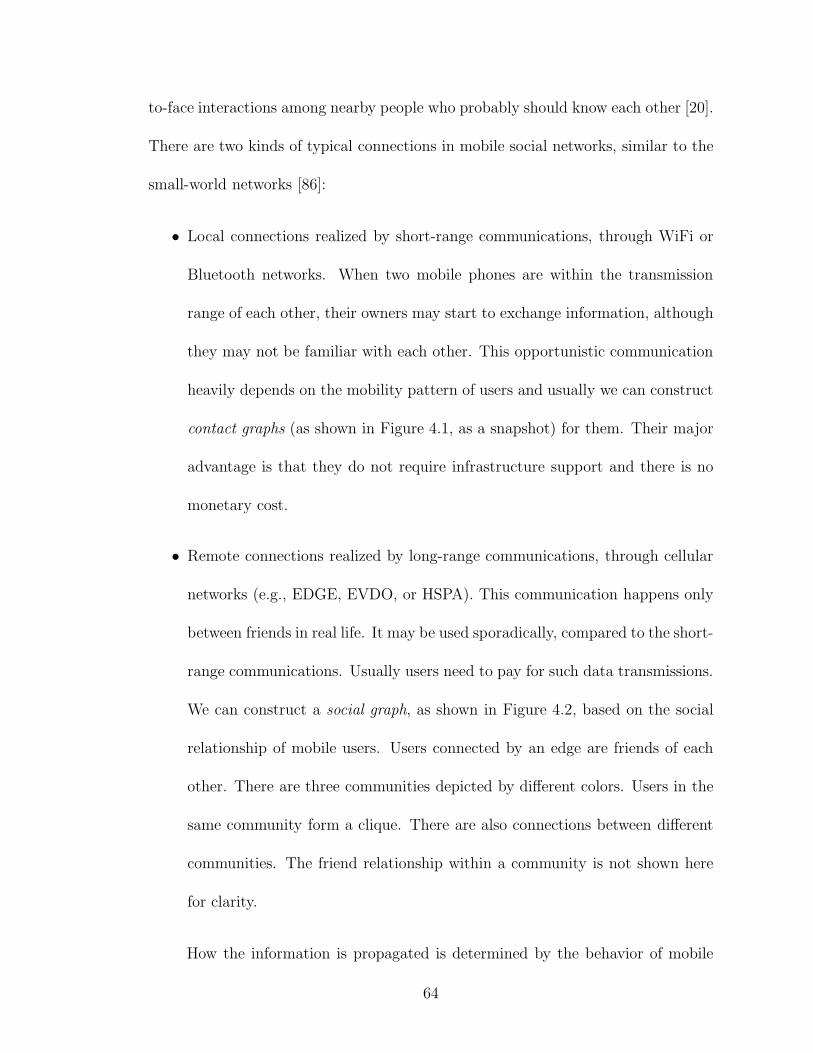
to-face interactions among nearby people who probably should know each other [20].

There are two kinds of typical connections in mobile social networks, similar to the

small-world networks [86]:

• Local connections realized by short-range communications, through WiFi or

Bluetooth networks. When two mobile phones are within the transmission

range of each other, their owners may start to exchange information, although

they may not be familiar with each other. This opportunistic communication

heavily depends on the mobility pattern of users and usually we can construct

contact graphs (as shown in Figure 4.1, as a snapshot) for them. Their major

advantage is that they do not require infrastructure support and there is no

monetary cost.

• Remote connections realized by long-range communications, through cellular

networks (e.g., EDGE, EVDO, or HSPA). This communication happens only

between friends in real life. It may be used sporadically, compared to the short-

range communications. Usually users need to pay for such data transmissions.

We can construct a social graph, as shown in Figure 4.2, based on the social

relationship of mobile users. Users connected by an edge are friends of each

other. There are three communities depicted by different colors. Users in the

same community form a clique. There are also connections between different

communities. The friend relationship within a community is not shown here

for clarity.

How the information is propagated is determined by the behavior of mobile

64

users, and we exploit a probabilistic dissemination model in this chapter. We define

the pull probability to be the probability that mobile users pull the information from

their peers during one of their contacts. The value of pull probability p may not

be the same for different types of information and might change as time goes on,

which reflects the dynamics of information popularity. After mobile users receive the

information from either the service providers or their peers, they may also forward

it, through cellular networks (e.g., MMS, Multimedia Messaging Service), to their

friends with probability q. Usually, p > q, because users may prefer the free op-

portunistic communications. Moreover, short-range communications consume much

less energy, in terms of data transmission, than long-range ones. For example, it

was reported in a measurement study that to download 10 KB data, WiFi consumes

one-sixth of 3G’s energy and one-third of GSM’s energy [6].

The modeling of information dissemination through opportunistic communi-

cations can be viewed as a combination of three sub-processes. First, to protect

their privacy, mobile users have the control of whether or not to share a piece of

information with their geographical neighbors and share it with probability p1. Sec-

ond, mobile users may want to explore the information in their proximity only when

they are not busy and mobile phones may not always be able to discover each other

during their short contacts. Thus they can find the meta-data of a piece of informa-

tion with probability p2. Finally, based on these meta-data, mobile users will decide

whether or not to fetch the information from their geographical neighbors and pull

it with probability p3. As a result, p = p1 · p2 · p3.

The rest of this chapter is organized as follows. We prove the submodularity

65

of information dissemination function in Section 4.2. In Section 4.3 we present two

centralized algorithms for the target-set selection problem in mobile content delivery.

We evaluate the performance of these two algorithms through extensive trace-driven

simulation studies in Section 4.4.

4.2 Submodularity of Information Dissemination Function

The information dissemination function is the function that maps the target set

to the expected number of infected users of the information dissemination process.

If we can prove that the information dissemination function is submodular, we can

then apply the well-known greedy algorithm proposed by Nemhauser et al. [65] to

identify the target set. For any subset S of the users, the information dissemination

function g(S) gives the final number of infected usres when S is the initial target

set. The function g(·) is submodular if it satisfies the diminishing returns rule. That

is, the marginal gain of adding a user, say u, into the target set S is greater than or

equal to that of adding the same user into a superset S ′ of S:

g(S ∪ u) − g(S) ≥ g(S ′ ∪ u) − g(S ′),

for all users u and all pairs of sets S ⊆ S ′. We prove the submodularity of the

information dissemination function by extending the approach developed in Kempe

et al. [45].

Our proof of the submodularity differs from that in Kempe et al. [45] in two

ways. First, Kempe et al. [45] prove that the information diffusion function is sub-

modular for the independent cascade model [33] of influence maximization. In that

66

model, when a node u becomes active, it has a single chance to activate any currently

inactive neighbor v with probability pu,v. In comparison, in our extended indepen-

dent cascade model, mobile users have the chance to pull/exchange information for

every contact. There are also several other diffusion models in the literature [84]

and some of them were derived from another basic model, the linear threshold

model [45]. Our enhanced independent cascade model is more realistic than these

previous models, as it can account for multiple contacts among mobile users.

Second, compared to the information diffusion in traditional social networks [45],

the contact graph of mobile social networks changes dynamically and mobile users

can pull information from their peers at every contact. To solve this problem, we

generate a time-stamped contact graph, which is also called time-expanded graph in

the literature, e.g., in Hoppe and Tardos [39]. Note that the delay-tolerance thresh-

old (i.e., the delivery deadline) determines the information dissemination duration

(from when service providers deliver information to target users to the delivery

deadline). As a result, only edges whose corresponding contacts occur before the

threshold will be included in this time-stamped graph.

Generally it is hard to compute exactly the underlying information dissemina-

tion function g(·) and obtain a closed form expression of it. However, as in Kempe

et al. [45], we can estimate the value of g(·) by Monte Carlo sampling. For each pair

of users u and v, if they are in contact ℓ times during the information dissemination

process, there will be ℓ time-stamped edges in the graph, one for each contact. Sup-

pose u’s pull probability for v during a given contact t is pu,v,t.2 We can view this

2We can define the pull probability pv,u,t accordingly.

67

random event as flipping a coin of bias pu,v,t. Note that whether we flip the coin at

the beginning of information dissemination or when u and v are in contact t will not

affect the final results. Thus, we can assume that for every contact t of each pair of

users u and v, we flip a coin of bias pu,v,t at the beginning of the process and save

the result to check later.

After we get all the results of coin flips, we mark the edges with successful

pulling of information as active and the remaining edges as inactive. Since we

already know the results of the coin flips (i.e., whether a mobile user can infect

his/her peers for a given contact) and the initial target set, we can calculate the

number of infected users at the end of the information dissemination process. In

fact, one possible set of results of the coin flips stands for a sample point in the

probability space. Suppose z is a sample point and define gz(S) to be the number of

infected users when S is the initial target set. Then gz(S) is a deterministic quantity

for a fixed contact trace. Further define I(u, z) to be the set of users that have a

path from u, for which all the edges on it are active and their time-stamps satisfy

the monotonically increasing requirement3. We have

gz(S) = ∪u∈SI(u, z).

We now prove that the function gz(S) is submodular for a given z. Consider

two sets S and S ′, S ⊆ S ′. gz(S ∪u)−gz(S) is the number of users in I(u, z) that

are not in ∪v∈SI(v, z). Note that ∪v∈S′I(v, z) is at least as large as ∪v∈SI(v, z). We

3This requirement reflects the temporal evolution of the information dissemination process along

the paths.

68

then have

gz(S ∪ u) − gz(S) ≥ gz(S′ ∪ u) − gz(S

′).

Since g(S) =∑

z Prob(z) · gz(S), we thus obtain that g(·) is submodular, because it

is a non-negative linear combination of a family of submodular functions.

4.3 Greedy and Heuristic Algorithms

We propose two algorithms for the target-set selection problem, called Greedy

and Heuristic. For the Greedy algorithm, initially the target set is empty. We

evaluate the information dissemination function g(u) for every user u, and select

the most active user (i.e., the one that can infect the largest number of uninfected

users) into the target set. Then we repeat this process, in each round selecting the

next user from the rest with the maximum increase of g(·) into the target set, until we

get the k users. Target-set selection is an NP-hard problem for both the independent

cascade model and the linear threshold model [45]. Let S∗ be the optimal target set,

Nemhauser et al. [65] show that if the function g(·) is non-negative, monotone and

submodular, and at each time we select a user that gives the maximum marginal

gain of g(·) to get a target set S with k users, then g(S) ≥ (1 − 1/e) · g(S∗). Thus,

given that the information dissemination function satisfies the above requirements,

the Greedy algorithm approximates the optimum solution to within a factor of

(1 − 1/e). However, we note that the limitation of the Greedy algorithm is that

it requires the knowledge of user mobility during the dissemination process, which

may not be available at the very beginning.

69

To make the Greedy algorithm practical, we propose to exploit the regularity

of human mobility [34, 58], which leads to the Heuristic algorithm. Based on a six-

month trace of the locations of 100,000 anonymized mobile phone users, Gonzalez et

al. [34] identify that human mobility shows a very high degree of temporal and spatial

regularity, and that each individual returns to a few highly frequented locations

with a significant probability. Benefiting from the regularity of human mobility,

the Heuristic algorithm identifies the target set using the history of user mobility,

and then uses this set for information delivery in the future. That is, for a given

period [s, t] of a day d, we apply the Greedy algorithm to determine the target

set S of the same history period [s, t] of the day d − c based on mobility history,

where c is a small integer (usually 1 or 2), and then for information delivery of [s, t]

of the day d, service providers send the information to mobile users in S at the

beginning to bootstrap the dissemination process. To enable the Greedy algorithm,

the information dissemination protocol can collect the contact information of the

subscribed users. At the end of a day, users can upload the information to the

service providers through either their PCs or the WiFi interfaces on their phones.

Finally, we also present the Random algorithm, as the baseline. In the Random

algorithm, the service providers select k target users randomly from all the sub-

scribed users. As we will show in Section 4.4, although this algorithm is simple,

it is still effective in the offloading process. Before presenting the simulation re-

sults, we introduce our prototype implementation in the next section, which verifies

the feasibility of mobile data offloading through opportunistic communications in

practice.

70

4.4 Simulation Studies

We now introduce the mobility traces that we use for performance evaluation,

and then present the results from a trace-driven simulator developed in C. The sim-

ulator first loads contact events from real-world traces or generates contact events

based on the movement history from the synthetic traces. It then replays the con-

tact events for the given information dissemination periods. At the beginning of

each contact, the simulator determines randomly whether a mobile user can get the

information from the peer based on the pre-configured pull probability.

4.4.1 Mobility Traces

4.4.1.1 Synthetic Mobility Trace

We use the SIGMA-SPECTRUM simulator [10] to generate a synthetic mo-

bility trace in the region of Portland, Oregon. The simulator combines different

real-world data sources and realistic models, including an urban mobility model,

synthetic population (according to U.S. Census data) and road-network data of

Portland. The trace records the location of mobile users every 30 seconds. We ran-

domly choose 10,000 people from the entire population of the city (around 1,600,000

people) as the subscribed users. The information dissemination periods start from

7:00AM with different durations. Note that the duration of the information dissem-

ination period is, in fact, also the delay-tolerance threshold for mobile users (i.e.,

the maximum delay they need to tolerate). We use this trace to evaluate the perfor-

mance of the Random algorithm for different pull probabilities and delay-tolerance

71

thresholds.

4.4.1.2 Traces From Real-World Experiments

To evaluate the performance of the Heuristic algorithm, we need the mobility

traces of different days, which is not available in the SIGMA-SPECTRUM simulator.

To this end, we exploit two real-world mobility traces from the Haggle project [12]

and the Reality Mining project [21].

We use the INFOCOM06 trace collected by the Haggle project for 4 days (from

2006-04-24 to 2006-04-27) during INFOCOM 2006 in Barcelona, Spain. This trace

recorded the mobility of students and researchers attending the student workshop,

using 78 iMotes which had a communication range of around 30 meters. We select

3 pairs of 1-hour periods from the trace as shown in Table 4.1. Thus, the delay-

tolerance threshold is 1 hour for this trace. To exploit the 24-hour regularity of

human mobility and evaluate the performance of the Heuristic algorithm, we use

the target set identified by the Greedy algorithm for the periods in the second

column (“History”) to predict the mobility of users for the periods in the third

column (“Delivery”) of the same row. We define active users as those who have at

least 1 contact with others during the delivery periods. As a result, the numbers of

active users for these periods are 70, 66 and 66. We can also use other thresholds

instead of 1. But they may exclude some inactive users for the simulation and thus

reduce the (already small) number of simulated users.

The Reality Mining trace was collected using 100 Nokia 6600 smartphones

72

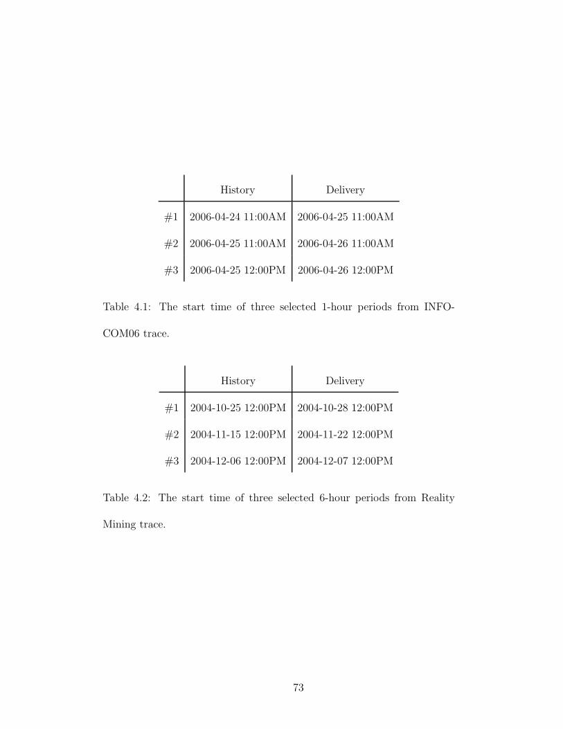
History Delivery

#1 2006-04-24 11:00AM 2006-04-25 11:00AM

#2 2006-04-25 11:00AM 2006-04-26 11:00AM

#3 2006-04-25 12:00PM 2006-04-26 12:00PM

Table 4.1: The start time of three selected 1-hour periods from INFO-

COM06 trace.

History Delivery

#1 2004-10-25 12:00PM 2004-10-28 12:00PM

#2 2004-11-15 12:00PM 2004-11-22 12:00PM

#3 2004-12-06 12:00PM 2004-12-07 12:00PM

Table 4.2: The start time of three selected 6-hour periods from Reality

Mining trace.

73

carried by people from the MIT Media Laboratory and Sloan Business School, from

2004-07-26 to 2005-05-05. The information in this trace includes call logs, neighbor-

ing Bluetooth devices, and associated cell-tower IDs, etc. The contact trace of these

users identified by the Bluetooth scanning is very sparse and thus is not suitable

for the simulation. As in Ioannidis et al. [42], we instead consider that two mobile

users are in contact of each other if their phones are associated with the same cell

tower. Even this cell-tower based contact trace is sparse: this is the reason that we

use 6-hour periods for the simulation. Therefore, the delay-tolerance threshold is

6 hours for this trace. Similar to Table 4.1, we show the 3 pairs of 6-hour periods

from the trace in Table 4.2. Benefiting from the long duration of the Reality Mining

project, we can also exploit the 3-day (#1 of Table 4.2) and 1-week (#2 of Table 4.2)

regularity of human mobility. The numbers of active users for these three periods

are 61, 71 and 53 for the Reality Mining trace. For both traces, we use only active

users in the simulation.

4.4.2 Simulation Results

In this section, we present the simulation results of the Random, Heuristic,

and Greedy algorithms. In the simulation, we emulate the information delivery of

multimedia newspapers (with size around several MB). Each direct cellular delivery

consumes one message containing the newspaper and for simplicity we assume there

is no further packetization. The simulated duration of a single run is determined

by the corresponding delay-tolerance threshold. Our goal here is to determine the

74

target set which leads to the most efficient mobile data offloading.

4.4.2.1 Pull Probability

We first evaluate the performance of Random algorithm for different pull prob-

abilities using the Portland trace. We show the mobile data traffic load for different

sizes of target set, from 5 to 3,000, and pull probabilities, 0.01, 0.05 and 0.1, in

Figure 4.3. The x-axis is the size of target set and the y-axis show the mobile traffic

load, in terms of the number of cellular messages. Every user who fails to receive the

information before the delivery deadline will consume a cellular message. Moreover,

each user in the target set will also consume a cellular message. The delivery dead-

line is 1 hour. For each combination of the size of target set and pull probability, we

run the simulation 10,000 times and report the average value. The horizontal dotted

line shows the amount of cellular messages without offloading, which is the same as

the total number of subscribed users. As we can see from this figure, even for the

very simple random algorithm, it can reduce the amount of mobile data traffic by

up to 81.42% when the pull probability is 0.1. When we reduce the pull probability

to 0.01, it can still offload mobile data traffic by up to 69.73%.

There are two main observations from this figure. First, the amount of mobile

data traffic decreases as the pull probability increases. It is because when mobile

users are all active in information propagation, a large number of users can get

the delivered information from their peers through opportunistic communications,

and thus avoid the data transmissions over cellular networks. Hence, active social

75

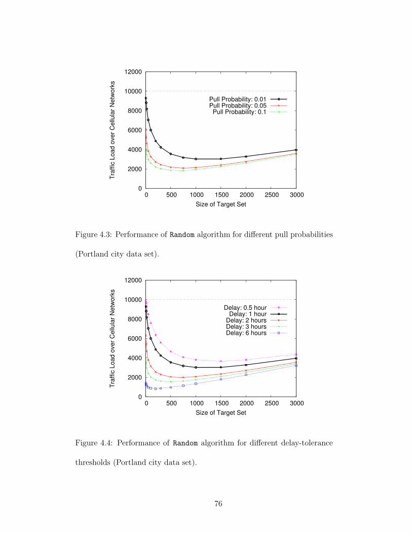
0

2000

4000

6000

8000

10000

12000

0 500 1000 1500 2000 2500 3000

Tra

ffic

Lo

ad

ove

r C

ellu

lar

Ne

two

rks

Size of Target Set

Pull Probability: 0.01Pull Probability: 0.05Pull Probability: 0.1

Figure 4.3: Performance of Random algorithm for different pull probabilities

(Portland city data set).

0

2000

4000

6000

8000

10000

12000

0 500 1000 1500 2000 2500 3000

Tra

ffic

Lo

ad

ove

r C

ellu

lar

Ne

two

rks

Size of Target Set

Delay: 0.5 hourDelay: 1 hour

Delay: 2 hoursDelay: 3 hoursDelay: 6 hours

Figure 4.4: Performance of Random algorithm for different delay-tolerance

thresholds (Portland city data set).

76

participation is a key enabling factor of efficient information delivery. Second, as

the size of target set increases, the amount of mobile data traffic first decreases

and then increases. The reasons are: (1). when the size of target set is small, the

expected number of users that can receive the information through opportunistic

communications is also small and thus a large number of users need to get the

information through cellular networks; (2). when the size of target set is large,

although it can make more users receive the information through opportunistic

communications, the users in the target set will directly generate a large amount of

mobile data traffic.

For the three curves in Figure 4.3, the pull probability is fixed for all the

contacts of these mobile users. We also tried different probabilities for different

contacts, uniformly and randomly selected between 0.01 and 0.1. The result looks

very similar to the curve with pull probability 0.05. Thus, we omit that result

for clarity. Note that, since information service providers will deliver information

to those users who cannot receive it before delay-tolerance threshold, the delivery

percentage is always 100% in our mobile data offloading solutions.

4.4.2.2 Delay-Tolerance Threshold

We then evaluate the performance of Random algorithm for different delay-

tolerance thresholds for the Portland trace. We show the traffic load over cellular

networks for five delay-tolerance thresholds, 0.5, 1, 2, 3 and 6 hours, in Figure 4.4,

as different types of data have different delay-tolerance requirements. The pull

77

probability is 0.01. We also run the simulation 10,000 times for a point in that

plot and report the average value. As we can see from this figure, if mobile users

are willing to tolerate longer delay we may be able to offload more traffic from

cellular networks. However, the benefit of increasing the delay-tolerance threshold

from 2 hours to 3 hours is not very significant, compared to that from 1 hour to

2 hours. One possible reason is that when we increase the threshold to 2 hours,

most of the active users can receive the delivered information through opportunistic

communications and thus the improvement of increasing it to 3 hours is limited.

4.4.2.3 Another Synthetic Mobility Trace

We also validate the simulation results about pull probability and delay-

tolerance threshold on a smaller synthetic mobility trace, again generated by the

SIGMA-SPECTRUM simulator [10]. This time, we randomly choose 1,000 people

around the Salt Lake City area as subscribed users. Other settings are similar to

those of the Portland trace. We plot the results in Figure 4.5 and Figure 4.6, which

show comparable trends as in Figure 4.3 and Figure 4.4.

4.4.2.4 Comparing Random, Heuristic, and Greedy

We compare the performance of Random, Heuristic and Greedy algorithms

using the two real-world traces. To verify the regularity of human mobility, we

show in Table 4.3 the IDs of the top 5 most active users for 2 pairs of selected

periods, for the INFOCOM06 trace and the Reality Mining trace. The numbers

78

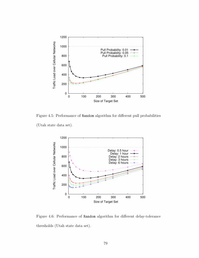
0

200

400

600

800

1000

1200

0 100 200 300 400 500

Tra

ffic

Lo

ad

ove

r C

ellu

lar

Ne

two

rks

Size of Target Set

Pull Probability: 0.01Pull Probability: 0.05Pull Probability: 0.1

Figure 4.5: Performance of Random algorithm for different pull probabilities

(Utah state data set).

0

200

400

600

800

1000

1200

0 100 200 300 400 500

Tra

ffic

Lo

ad

ove

r C

ellu

lar

Ne

two

rks

Size of Target Set

Delay: 0.5 hourDelay: 1 hour

Delay: 2 hoursDelay: 3 hoursDelay: 6 hours

Figure 4.6: Performance of Random algorithm for different delay-tolerance

thresholds (Utah state data set).

79

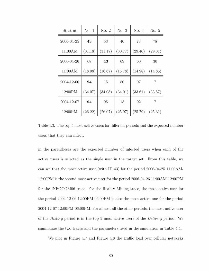
Start at No. 1 No. 2 No. 3 No. 4 No. 5

2006-04-25 43 53 40 73 78

11:00AM (31.18) (31.17) (30.77) (29.46) (29.31)

2006-04-26 68 43 69 60 30

11:00AM (18.08) (16.67) (15.78) (14.98) (14.86)

2004-12-06 94 15 80 97 7

12:00PM (34.07) (34.03) (34.01) (33.61) (33.57)

2004-12-07 94 95 15 92 7

12:00PM (26.22) (26.07) (25.97) (25.79) (25.31)

Table 4.3: The top 5 most active users for different periods and the expected number

users that they can infect.

in the parentheses are the expected number of infected users when each of the

active users is selected as the single user in the target set. From this table, we

can see that the most active user (with ID 43) for the period 2006-04-25 11:00AM-

12:00PM is the second most active user for the period 2006-04-26 11:00AM-12:00PM

for the INFOCOM06 trace. For the Reality Mining trace, the most active user for

the period 2004-12-06 12:00PM-06:00PM is also the most active one for the period

2004-12-07 12:00PM-06:00PM. For almost all the other periods, the most active user

of the History period is in the top 5 most active users of the Delivery period. We

summarize the two traces and the parameters used in the simulation in Table 4.4.

We plot in Figure 4.7 and Figure 4.8 the traffic load over cellular networks

80

Haggle MIT Reality

Trace INFOCOM06 Mining

Network type Bluetooth Bluetooth

Device type iMote Nokia 6600

Number of devices 78 100

Duration of trace 4 days 9 months

Regularity 1 day 1, 3, 7 days

Simulated duration 1 hour 6 hours

Pull probability 0.01 0.001

# of Active users ≤ 70 ≤ 71

Table 4.4: Summary of two real-world traces.

81

for the 6 pairs of periods listed in Table 4.1 and Table 4.2. Due to the small

number of mobile users in the traces, we set the size of target set to be 5. For

the Random and Heuristic algorithms, we simulate the information dissemination

process 100,000 times and report the averaged values. For the Greedy algorithm, we

run the simulation 10,000 times to determine the marginal gain for each user. After

we identify the target users, we also run the simulation 100,000 times and report

the averaged values. In these figures, the Base shows the amount of mobile data

traffic without offloading, which is the same as the number of active users during

these periods.

The performance of these algorithms depends on the pull probability. The

pull probability is 0.01 for the INFOCOM06 trace and 0.001 for the Reality Mining

trace. For high pull probabilities, there is no significant difference among them. As

we can see from these figures, Greedy performs the best, followed by the Heuristic

algorithm, for all the cases. Compared to the Base, the Random algorithm can

reduce the amount of mobile data traffic by up to 53.91% for the INFOCOM06

trace and 70.72% for the Reality Mining trace. Owing to the regularity of human

mobility, Heuristic can further reduce the amount of mobile data traffic of Random

by up to 18.95% for the INFOCOM06 trace and 12.25% for the Reality Mining

trace. Although Greedy and Heuristic perform better than Random, the difference

is not very significant. One of the possible reasons is that due to the small number

of mobile users and their limited active area, even if we choose the target users

randomly, with high probability the information will be disseminated to some very

active users quickly, who will then affect a large number of other users. Compared to

82

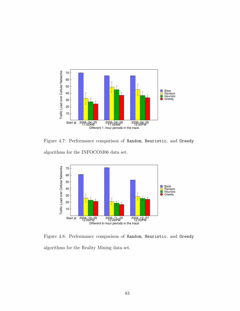
10

20

30

40

50

60

70

2006−04−2511:00AM

2006−04−2611:00AM

2006−04−2612:00PM

Tra

ffic

Lo

ad

ove

r C

ellu

lar

Ne

two

rks

Different 1−hour periods in the trace

Start at

BaseRandomHeuristicGreedy

Figure 4.7: Performance comparison of Random, Heuristic, and Greedy

algorithms for the INFOCOM06 data set.

10

20

30

40

50

60

70

2004−10−2812:00PM

2004−11−2212:00PM

2004−12−0712:00PM

Tra

ffic

Lo

ad

ove

r C

ellu

lar

Ne

two

rks

Different 6−hour periods in the trace

Start at

BaseRandomHeuristicGreedy

Figure 4.8: Performance comparison of Random, Heuristic, and Greedy

algorithms for the Reality Mining data set.

83

the Greedy and Heuristic algorithms, a unique advantage of the Random algorithm

is that information service providers can avoid collecting the contact information

from subscribed users, which may make them feel comfortable to participate in the

information dissemination.

We note that due to the incompleteness of the real-world traces (e.g., caused

by hardware errors), some users in the target set of the History period may not

be active during the Delivery period (i.e., they have no contacts with other users

for the delivery period). In these cases, we replace them with randomly selected

users. We have not evaluated how the push-based approach can help the information

dissemination among friends, because there is no information about the social graph

of mobile users for the above traces. However, we note that it is possible to construct

the graph through the analysis of traffic between mobile users [93], or historical data

of mobile users, such as proximity and location at a given time [21]. We leave the

evaluation of push-based approach as a future work.

84

Chapter 5

Random-Walk Based Sampling

5.1 Introduction

In this chapter, we address the following question: how do we identify influ-

ential users in mobile social networks through distributed solutions with low control-

message overhead? There are two practical requirements when finding these critical

users in mobile settings. First, because these proposed protocols usually run on

battery-supported mobile devices, such as smartphones, we need to control their

communication overhead, as data transmission is the major source of energy con-

sumption on mobile devices. Second, given the large size of mobile social networks,

the proposed solutions should be distributed. Most centralized algorithms require

the complete contact graphs of mobile users and sending the updates of dynamic

contact graphs may introduce extra communication overhead. Moreover, centralized

schemes are known to have high computational complexity, especially on large social

graphs. For example, as reported by Chen et al. [14], finding a small set of nodes

with high centrality in a graph with 15,000 vertices could take days on a modern

server machine.

Our distributed approach is motivated by the “friendship paradox” [26] that

“your friends have more friends than you do” and leverages random-walk probe

messages to sample mobile users and thus to identify critical users. The reason

85

behind this paradox is that people with a large number of friends may have a

high probability of being observed among one’s friend circle. Thus, the friends of

randomly selected individuals may have higher centrality in friendship graphs than

average. Although the original proof in Feld [26] is for the static friendship graph of

traditional social networks, we can easily extend it for the dynamic contact graph

of mobile social networks.

Besides the mobile content delivery application, we demonstrate that we can

also benefit from the identified influential users for other applications, such as tar-

geted immunization and outbreak detection of infectious diseases.

The rest of this chapter is organized as follows. We model the dynamically

changing social-contact graphs using probabilistic temporal graphs in Section 5.2. In

Section 5.3, we present the distributed random-walk sampling protocol and provide

the theoretical analysis on static graphs. We demonstrate the effectiveness of the

identified influential users for hybrid mobile content delivery in Section 5.4 and for

targeted immunization in Section 5.5.

5.2 Probabilistic Temporal Graphs

Graph theory has been widely examined to study complex social networks,

which uses edges to reflect relationships between individuals, locations or organi-

zations [14, 25]. In these models, the temporal nature of dynamic social networks

is often overlooked, as in practice it is hard to get rich temporal information for

large-scale social networks and relationships in some social networks may evolve

86

very slowly. Thus, we usually study a snapshot of these networks, where the edges

are aggregated into a single static graph [45], and only a few works consider the

time-evolving nature of social graphs [51].

It has been a challenging problem to build reasonable and realistic models to

capture the contact patterns of mobile social networks. Compared with relation-

ship graphs in traditional social networks, contact graphs of mobile social networks

may change very fast over time due to human mobility. Moreover, by taking into

consideration the technical issues of realistic applications, such as information dis-

semination, mobile users may not always be able to exchange information during

their contacts. Also, in reality infectious diseases cannot spread among individuals

during all their contacts.

Consider the following simple example of information exchange between three

students, Alice, Bob and Carol, in a campus. Alice and Bob meet with each during a

class in the morning from 09:00:00 to 09:50:00, and Bob and Carol meet on a shuttle

from 14:30:00 to 14:40:00 in the afternoon of the same day. In the static contact

graph, there is an edge between Alice and Bob and another between Bob and Carol.

Thus, we can find a path between Alice and Carol through Bob. However, it is

possible only for Alice to forward her information to Carol and the other direction

of information flow along this path is not feasible on the same day. Carol can only

forward information to Alice during their contact on the next day from 22:10:30 to

22:12:30, in the hallway of their dormitory.

Although it is straightforward to state, the above observations add more com-

plications for the analysis of information dissemination in mobile social networks.

87

Temporal graph models have been recently proposed to encode temporal data into

graphs and meanwhile retain the temporal nature of original data [48]. As the first

step to model the temporal nature of social contacts, there are two limitations of

this model when applying it for our purpose: (a) the considered temporal events

have no duration, which is not valid for face-to-face contacts of mobile users; (b) it

is unclear how to encode the probabilistic information into graphs.

We model social contacts using an undirected graph G = V, E, T, T, P,

where V is the set of users, the first T is the start time of an edge and the second is

the end time, and P is the probability space. Each edge in E, e = 〈u, v, ts, td, pe〉,

represents a possible event between mobile users u and v during their contact from

ts to td with a certain probability pe. The events could be exchanges of information

or infections of a disease during its outbreak. We show in Figure 5.1 the probabilistic

temporal graph of the above example.

As we mentioned above, the time dependency of edges in social-contact graphs

plays a vital role in information dissemination [38]. Information can flow from

e1 = 〈u1, v1, ts1, td1, pe1〉 to e2 = 〈u2, v2, ts2, td2, pe2〉 if and only if td1 > ts2 and

e1 and e2 share a common vertex. The same is true for the spread of infectious

diseases. We base our simulation studies of infectious disease control and information

dissemination in Sections 5.5 and 5.4 on this probabilistic temporal graph model.

88

Alice

Bob

Carol

D1 09:00:00D1 09:50:000.01

D1 14:30:00D1 14:40:000.005

D2 22:10:30D2 22:12:300.001

Figure 5.1: The social-contact graph for information exchange of three users, Alice,

Bob and Carol. The durations of these three contacts are 50, 10 and 2 minutes with

pe 0.01, 0.005 and 0.001.

5.3 The Random-Walk Sampling Protocol

In this section, we present the details of iWander design, offer its theoretical

analysis on static graphs, and discuss its proof-of-concept prototype implementation.

5.3.1 The Protocol

We propose to leverage random walks to design a distributed protocol, iWander,

for identifying influential users in mobile social networks. The intuition is that if

we periodically initialize random-walk probe messages from a small group of mobile

devices, influential users may be visited by these probe messages more frequently

than average.

The proposed iWander protocol works as follows. Every ∆T hours, iWander

89

generates a tiny probe message with a given probability q on each mobile device

and saves it in the device’s local queue. The message contains only a pre-configured

hop-limit field L. During the contacts of a mobile device with its peers, if it has a

probe message in its queue, it sends this message to another uniformly and randomly

selected peer. When a mobile device receives a probe message, it decreases L in the

message by 1, and then stores it in its local queue, waiting for the opportunity to

forward the message to other peers. A probe message with L = 0 will be finally

discarded. iWander maintains a random-walk counter on each mobile device, ini-

tialized to zero, to record how many times it has received the probe messages (i.e.,

visited by these random-walk messages).

After collecting the random-walk counters from all users recorded by their

mobile devices, we can determine the set of k critical users from the head of the user

list sorted by these counters. The reason is that based on the friendship paradox,

influential users have high probabilities to be visited by random walks and thus own

large random-walk counters.

Differently from the random-walk betweenness metric proposed by Newman [66],

iWander applies fixed-length instead of all-pairs random walks for two reasons. First,

in practice, it is difficult for a mobile user to know every other user and thus specify

the random-walk destination of probe messages. Second, the message overhead of

all-pairs random walks may be much higher than fixed-length random walks, which

makes them unsuitable for battery-powered mobile devices.

The update and reset of random-walk counters are determined by the upper

layer applications. In practice, they may reset these counters periodically, for ex-

90

ample, at midnight (12:00 AM) of every day. They can also apply an exponential

moving average to update these counters by assigning a higher weight to recent

counters.

In summary, the performance of iWander relies on three parameters: q – the

probability that a mobile device generates a random-walk probe message, L – the

length of random walks performed by probe messages (i.e., the number of mobile

users visited by a single probe message), and ∆T – the frequency of generating new

random-walk probe messages. It is important to understand the impact of these

three parameters on the performance of iWander, because they determine both the

quality of identified influential users and the number of probe messages spreading

over the network.

5.3.2 Theoretical Analysis

We analyze the parameter L of our protocol on static graphs. To reduce

energy consumption on mobile devices, we prefer short random walks with only a

few steps. “Static” versions of social-contact networks are often very dense and

expander-like. In such highly-mixing networks, we prove that a random walk of

length O(log n), where n is the number of nodes in the network, suffices to come

very close to the stationary distribution of the random walk (in which each vertex

has a probability proportional to its degree). Thus, the short random walks that

we take will likely come quite close to sampling vertices approximately according to

their degrees, because the static snapshots of dynamic mobile networks will likely

91

be expander-like.

Let n be the number of nodes and m be the number of edges in the graph

G(V, E), which refers to a static version of the dynamic graph. Let d(v) be the degree

of vertex v and d(S) =∑

v∈S d(v) for any S ⊆ V . Suppose A is the adjacency matrix

of G and D is the diagonal matrix diag( 1d(v1)

, . . . , 1d(vn)

). Suppose λ1 ≥ λ2 ≥ . . . λn

are the eigenvalues of the symmetric matrix N = D1/2AD1/2. We assume the graph

is an expander graph, which means the mixing rate λ = min(|λ2|, |λn|) of G is a

constant less than 1 [55]. There are several other definitions of expander graphs,

such as vertex expansion or edge expansion, and they are more or less equivalent to

each other.

Before proving the main theorem, we present the following well-known fact

(see, e.g., Lovasz [55]).

Lemma 1 Consider several independent random walks starting at arbitrary nodes.

Let Pi,t(v) be the probability that the ith random walk visits v at time t and let

Pi,t(S) =∑

v∈S Pi,t(v). The stationary distribution of the random walk is π. We

have that

|Pi,t(S) − π(S)| ≤√

d(S)λt.

It is well known that the stationary distribution of a random walk is proportional

to the degree distribution of the graph. More specifically, π(v) = d(v)2m

.

Initially, we choose αn nodes to generate random-walk probe messages where

α is a positive number between 0 and 1. After all random-walk probe messages

run L steps, we select βn vertices with the highest random-walk counters. Denote

92

this set by S and the set of βn vertices with the highest degrees by S∗. Here, α is

essentially the same as q (the probability to generate random-walk probe messages)

and β is an input parameter whose value depends on the upper layer applications.

We show that with high probability, the total degree of the chosen set S is close to

that of the optimal set S∗.

Theorem 1 For any constant α, β, ǫ > 0 and sufficiently large n, after L = 10ǫβ

log 1

λ

n =

O(log n) steps, we have that

Pr[d(S) ≥ (1 − ǫ)d(S∗)] ≥ 1 −1

exp(Ω(n))

Proof: Consider a particular vertex v ∈ V . Let Ii,t(v) be the indicator random

variable that the ith random walk visits v at time t. Denote the random-walk

counter of v at time t by Ct(v). We can easily see from our proposed protocol that

Ct(v) =∑αn

i=1

∑tt′=1 Ii,t′(v). By linearity of expectation,

E[Ct(v)] =

αn∑

i=1

t∑

t′=1

E[Ii,t′(v)] =∑

i

∑

t′≤t

Pi,t′(v)

Consider a random walk i. By Lemma 1, we can see that for any S ′ ⊆ V ,

∣

∣

∑

t′≤t

Pi,t′(S′) − π(S ′) · t

∣

∣ ≤∑

t′≤t

|Pi,t′(S′) − π(S ′)|

=∑

t′≤log 1

λ

n

|Pi,t′(S′) − π(S ′)|

+∑

log 1

λ

n≤t′≤t

|Pi,t′(S′) − π(S ′)|

≤ log 1

λ

n +√

d(S ′)λ

log 1

λ

n

1 − λ≤ 2 log 1

λ

n

Therefore, we obtain that for any S ′ ⊆ V ,

|E[Ct(S′)] − αntπ(S ′)| ≤ 2αn log 1

λ

n.

93

Letting L = 10ǫβ

log 1

λ

n, we have 2αn log 1

λ

n ≤ ǫ4αnLβ ≤ ǫ

4αnLπ(S∗) and

E[CL(S∗)] ∈ [(1 ±ǫ

5)αnLπ(S∗)]. (5.1)

Since all random walks are independent of each other, using Chernoff bound, we

can get that

Pr[

|Ct(S∗) ∈ [(1 ±

ǫ

5)E[Ct(S

∗)]]

≥ 1 − 2 exp(−E[Ct(S

∗)]ǫ2

75t)

= 1 −1

exp(Ω(n))(5.2)

Combining (5.1) and (5.2), we get

Pr[

Ct(S∗) ∈ [(1 ±

ǫ

2)αntπ(S∗)]

]

≥ 1 − 2 exp(−E[Ct(S

∗)]ǫ2

75t)

≥ 1 −1

exp(Ω(n))(5.3)

Similarly, we can get that

Pr[

Ct(S) ∈ [(1 ±ǫ

2)αntπ(S)]

]

≥ 1 −1

exp(Ω(n))(5.4)

From (5.3) and (5.4) and the fact that Ct(S) ≥ Ct(S∗) and π(S∗) ≥ π(S), we can

get

Pr[

|π(S∗) − π(S)| ≤ ǫπ(S∗)]

≥ 1 −1

exp(Ω(n))

Noting that π(S) = d(S)/2m, we complete the proof. 2

We note that compared with the degree-based scheme for identifying influential

mobile users, one of the attractive features of our random-walk sampling is its low

control-message overhead, which is verified in Section 5.5.

94

We leave the theoretical analysis of random walks on dynamic graphs for our

future work. Recently, Figueiredo et al. [27] study the steady state distribution of

continuous-time random walks on dynamic graphs, which are stationary and ergodic,

and may vary over time. They characterize this distribution under several cases,

e.g., the walker rate is much faster or slower than the changing rate of the graph, or

the rate is proportional to the node degree at each step of a random walk. In our

model, since mobile devices perform device discovery periodically, we are interested

in discrete-time random walks on dynamic graphs.

In Section 5.5.2, we investigate how the length of random walks L affects the

performance of iWander through trace-driven simulation studies. We also evaluate

the performance of iWander with different probabilities (q) and frequencies (∆T ) of

the generation of random-walk probe messages.

5.3.3 Proof of Concept

To demonstrate the feasibility of iWander, we implement a prototype in C

language on Nokia N900 smartphones. We choose Bluetooth as the underlying

communication protocol for iWander due to its low energy consumption. We mea-

sured the power of discovery and idle modes of Bluetooth and WiFi devices and

summarize the average results and standard deviations for 10 runs in Table 5.1,

which shows that in Bluetooth discovery mode the power of N900 is less than 1/3

of WiFi discovery. Moreover, when the Bluetooth device is in idle mode, the power

of N900 is negligible. The reason for high power of WiFi idle mode is that to en-

95

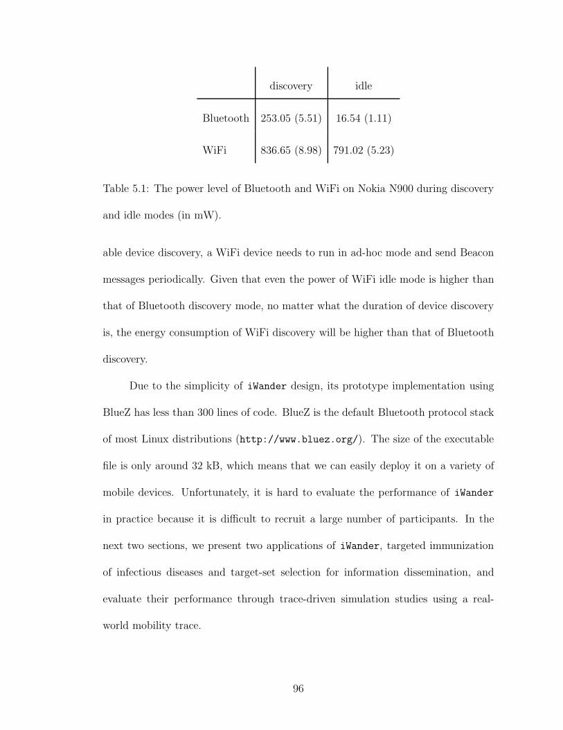
discovery idle

Bluetooth 253.05 (5.51) 16.54 (1.11)

WiFi 836.65 (8.98) 791.02 (5.23)

Table 5.1: The power level of Bluetooth and WiFi on Nokia N900 during discovery

and idle modes (in mW).

able device discovery, a WiFi device needs to run in ad-hoc mode and send Beacon

messages periodically. Given that even the power of WiFi idle mode is higher than

that of Bluetooth discovery mode, no matter what the duration of device discovery

is, the energy consumption of WiFi discovery will be higher than that of Bluetooth

discovery.

Due to the simplicity of iWander design, its prototype implementation using

BlueZ has less than 300 lines of code. BlueZ is the default Bluetooth protocol stack

of most Linux distributions (http://www.bluez.org/). The size of the executable

file is only around 32 kB, which means that we can easily deploy it on a variety of

mobile devices. Unfortunately, it is hard to evaluate the performance of iWander

in practice because it is difficult to recruit a large number of participants. In the

next two sections, we present two applications of iWander, targeted immunization

of infectious diseases and target-set selection for information dissemination, and

evaluate their performance through trace-driven simulation studies using a real-

world mobility trace.

96

5.4 Facilitating Mobile Content Delivery

In this section, we illustrate how to benefit from iWander for target-set selec-

tion in mobile content delivery. We employ opportunistic communications and social

participation to facilitate information dissemination and thus reduce the amount of

data traffic in cellular networks.

5.4.1 Target-Set Selection Using Random Walks

The centralized greedy and heuristic algorithms require the complete social-

contact graph of a given time period and share the same computational inefficiency

as the original greedy algorithm by Kempe, Kleinberg, and Tardos [45]. To solve

these problems, we leverage the random-walk counters of iWander to select target

users without requiring global network structure and thus design a distributed so-

lution for the target-set selection problem. Mobile devices attached with users run

iWander in the background and periodically report their random-walk counters to

a centralized server of information service providers. The providers then sort all

users based on these counters and choose the top-k users into the target set. In this

scenario mobile users not in the target set can also help to propagate information

once they receive it from either target users or others.

The process of information dissemination in mobile social networks is mainly

determined by user behaviors. Usually, mobile devices can start the exchange of

information after they know each other through periodic device discovery. A key

concept in the target-set selection problem is the information dissemination prob-

97

ability and it is defined as the probability p that information propagates among

mobile users after each device discovery. The value of p may be affected by several

factors, including status of mobile users and their privacy concerns. Mobile users

with high levels of privacy concerns or those who are very busy with their work may

have a low probability to involve in information dissemination process. Similar to

the transmission of infectious diseases, given the value of p, the probability that two

mobile users with a 60-second device discovery interval can exchange information

during a t-second contact is 1 − (1 − p)⌊t/60⌋.

We note that the purpose of target-set selection for mobile information dissem-

ination is different from targeted immunization, although the usage of random-walk

counters is similar in these two applications. For targeted immunization, we want

to vaccinate all influential individuals as early as possible. For target-set selection,

as we will show in Section 5.4.2.2, adding non-influential users into the target set

can increase the number of infected users for large target sets.

5.4.2 Performance Evaluation

We develop another trace-driven simulator also in C, using the same Dart-

mouth data set [49], to evaluate the performance of random-walk based target-set

selection. In this simulator, we assume that the underlying wireless communication

is reliable. We have measured the performance of Bluetooth-based opportunistic

communications on Nokia N900 smartphones, such as the device discovery proba-

bility [38]. We are currently working on a packet-level simulator to take into account

98

the low layer issues, including the failure of random-walk probe messages and the

transmission of data packets in information dissemination.

5.4.2.1 Simulation Setup

The simulator first generates the contacts trace of mobile users under the

same assumption that they are in contacts if their wireless devices are associated

with the same access point. It then replays the contact events for the given infor-

mation dissemination period, from 12:00PM to 15:00PM on 2004-03-01.1 Based on

the pre-configured information dissemination probability, the simulator determines

randomly whether a user can receive information from peers after each device dis-

covery. We also call the users that can receive information before delivery deadline

infected users. Usually, information providers will send information to uninfected

users at the end of dissemination period, to guarantee that every user can finally

receive the delivered information [38].

We compare the performance of random-walk based target-set selection, RW-1,

with random selection, Random, and the degree-based selection, Degree. The in-

terval of device discovery is 60 seconds, which means that mobile devices have the

chance to start the exchange of information every 60 seconds. Similar to degree-

based immunization, Degree also uses the number of other devices that a mobile

device has contacted with as the metric to select target users. For RW-1, mobile

devices generate 1-step random-walk probe messages of iWander with probability

1We have also evaluated other information dissemination periods with different dura-

tions and got similar results with those presented in this chapter.

99

0.1 every hour. RW-1 and Degree choose target users based on the updated random-

walk counters and the number of contacts of mobile devices at the beginning of

information dissemination period. We refer interested readers to Han et al. [38] for

the performance evaluation of the centralized greedy and heuristic algorithms.

5.4.2.2 The Amount of Cellular Data Traffic

We plot the normalized amount of cellular data traffic for RW-1, Random and

Degree in Figure 5.2. In these subfigures, the y-axis value is normalized over the

amount of cellular data traffic of a baseline scheme, in which information service

providers send content to every user through cellular unicast delivery. We run the

simulation 1,000 times and report the average values with standard deviations. The

information dissemination probability p is 0.01, 0.05 and 0.005 for Figures 5.2a, 5.2b

and 5.2c. We vary the size of target set from 10 to 2,000. As we can see from these

subfigures, RW-1 and Random outperform Degree when the size of target set is larger

than 10. RW-1 performs better than Random for small target sets. For example, for

a target set with 50 users, RW-1 can deliver information to 51% more users than

Random (667 vs. 441) when p is 0.005. The improvement is 37% when p is 0.01

(1054 vs. 772) and 14% when p is 0.05 (1863 vs. 1639). Thus, RW-1 can reduce more

cellular data traffic than Random.

The performance of RW-1 becomes worse than Random for large target sets. One

of the possible reasons is that non-influential users (i.e., users with low centrality in

social-contact networks) also play an important role in information dissemination.

100

0

0.2

0.4

0.6

0.8

1

0 400 800 1200 1600 2000

Norm

aliz

ed c

ellu

lar

data

tra

ffic

Number of initial target users

DegreeRW-1

RandomMix-1

(a) p: 0.01

0

0.2

0.4

0.6

0.8

1

0 400 800 1200 1600 2000

Norm

aliz

ed c

ellu

lar

data

tra

ffic


DegreeRW-1

RandomMix-1

(b) p: 0.05

0

0.2

0.4

0.6

0.8

1

0 400 800 1200 1600 2000

Norm

aliz

ed c

ellu

lar

data

tra

ffic


DegreeRW-1

RandomMix-1

(c) p: 0.005

Figure 5.2: Comparison of the normalized cellular data traffic for four target-set

selection schemes with different values of p.

101

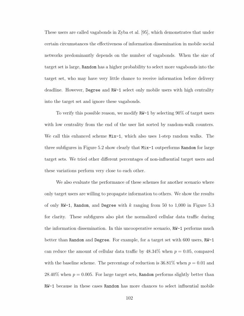
These users are called vagabonds in Zyba et al. [95], which demonstrates that under

certain circumstances the effectiveness of information dissemination in mobile social

networks predominantly depends on the number of vagabonds. When the size of

target set is large, Random has a higher probability to select more vagabonds into the

target set, who may have very little chance to receive information before delivery

deadline. However, Degree and RW-1 select only mobile users with high centrality

into the target set and ignore these vagabonds.

To verify this possible reason, we modify RW-1 by selecting 90% of target users

with low centrality from the end of the user list sorted by random-walk counters.

We call this enhanced scheme Mix-1, which also uses 1-step random walks. The

three subfigures in Figure 5.2 show clearly that Mix-1 outperforms Random for large

target sets. We tried other different percentages of non-influential target users and

these variations perform very close to each other.

We also evaluate the performance of these schemes for another scenario where

only target users are willing to propagate information to others. We show the results

of only RW-1, Random, and Degree with k ranging from 50 to 1,000 in Figure 5.3

for clarity. These subfigures also plot the normalized cellular data traffic during

the information dissemination. In this uncooperative scenario, RW-1 performs much

better than Random and Degree. For example, for a target set with 600 users, RW-1

can reduce the amount of cellular data traffic by 48.34% when p = 0.05, compared

with the baseline scheme. The percentage of reduction is 36.81% when p = 0.01 and

28.40% when p = 0.005. For large target sets, Random performs slightly better than

RW-1 because in these cases Random has more chances to select influential mobile

102

0

0.2

0.4

0.6

0.8

1

0 200 400 600 800 1000

Norm

aliz

ed c

ellu

lar

data

tra

ffic


DegreeRandom

RW-1

(a) p: 0.01

0

0.2

0.4

0.6

0.8

1

0 200 400 600 800 1000

Norm

aliz

ed c

ellu

lar

data

tra

ffic


DegreeRandom

RW-1

(b) p: 0.05

0

0.2

0.4

0.6

0.8

1

0 200 400 600 800 1000

Norm

aliz

ed c

ellu

lar

data

tra

ffic


DegreeRandom

RW-1

(c) p: 0.005

Figure 5.3: Comparison of the normalized cellular data traffic for three target-

set selection schemes with different values of p. Only target users can propagate

information to others.

103

users into a target set.

Differently from targeted immunization, increasing the values of q, L, or ∆T

has limited impact on the performance of random-walk based target-set selection.

We omit these results due to the limited space.

5.4.2.3 Delivery Delay

We finally compare the delivery delay of these four target-set selection schemes

for the cooperative scenario. We set the delivery delay of target users to be 0 and the

users who cannot receive information before delivery deadline to be 10,800 seconds,

the same as the duration of information dissemination period. We plot the delivery

delay for different information dissemination probabilities in Figure 5.4. Similarly to

the observation from Figure 5.2, RW-1 performs better than Random for small target

sets and Mix-1 outperforms Random for large target sets, in terms of delivery delay.

Moreover, they all perform better than Degree when the size of target set is larger

than 50.

In summary, when information service providers can deliver information di-

rectly to only a small number of users, we should use the pure random-walk based

target-set selection policy. However, the enhanced scheme that mixes both influen-

tial and non-influential users into the target set is preferable when it is possible to

deliver information to a large number of users directly.

104

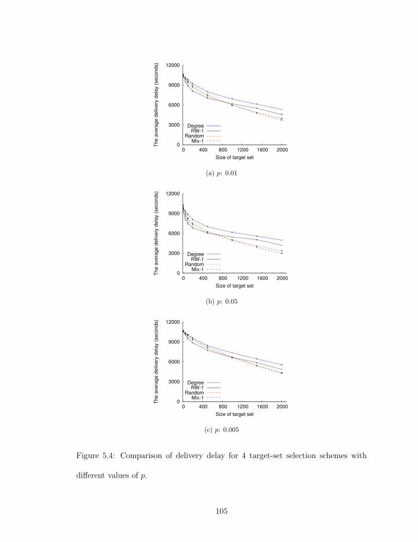
0

3000

6000

9000

12000

0 400 800 1200 1600 2000

The a

vera

ge d

eliv

ery

dela

y (

seconds)

Size of target set

DegreeRW-1

RandomMix-1

(a) p: 0.01

0

3000

6000

9000

12000

0 400 800 1200 1600 2000

The a

vera

ge d

eliv

ery

dela

y (

seconds)

Size of target set

DegreeRW-1

RandomMix-1

(b) p: 0.05

0

3000

6000

9000

12000

0 400 800 1200 1600 2000

The a

vera

ge d

eliv

ery

dela

y (

seconds)

Size of target set

DegreeRW-1

RandomMix-1

(c) p: 0.005

Figure 5.4: Comparison of delivery delay for 4 target-set selection schemes with

different values of p.

105

5.5 Controlling Infectious Diseases

In this section, we demonstrate how to utilize the critical individuals identified

by iWander to control infectious diseases and perform early outbreak detection.

5.5.1 Random-Walk Based Immunization

Mobile devices have recently been used to collect data pertaining to the be-

havior of individuals for various purposes, including disease control and health care.

For example, the FluPhone (https://www.fluphone.org/) study collects informa-

tion on social encounters in Cambridge, UK using mobile phones, with the goal of

helping medical researchers to better understand the propagation of close-contact

infections. Pollak et al. [75] design a mobile phone based game to motivate children

to practice healthy eating habits.

We propose to perform targeted immunization of infectious diseases based

on the random-walk counters maintained by iWander. For example, during the

flu season, iWander can periodically report these counters on the smartphones of

college students to the university health center. The medical staff can then vaccinate

students with high random-walk counters first to contain the spread of flu. We can

also use these counters to detect the outbreaks of infectious diseases, where the

medical staff monitor the health condition of students with high counters instead of

randomly selected students.

The centralized collection of random-walk counters is required by this spe-

cific application and the target-set selection for mobile information dissemination

106

in Section 5.4. For other applications, such as distribution of self-generated content

among users, it is possible to extend iWander and design a fully distributed proto-

col to compute and disseminate these counters among mobile users, for example, by

leveraging diffusing computations [18].

There are several differences between our proposed targeted immunization

scheme and those in the literature, for example, by Christakis and Fowler [15] and

Christley et al. [16]. First, our scheme can benefit from the social contacts de-

tected directly by mobile devices, instead of using the estimation through friendship

graphs generated from surveys [15]. Second, our scheme can reflect the dynamics

of social contacts in a timely way and avoid the computation-extensive centralized

data analysis. Finally, our fixed-length random-walk metric is an extension of the

general all-pairs random-walk betweenness centrality [66] and the one-step diffusion-

style estimation of node centrality [15], and its low control message overhead makes

it amenable to be run on mobile devices.

5.5.2 Performance Evaluation

We evaluate the performance of iWander for infectious disease control through

extensive trace-driven simulations.

5.5.2.1 Simulation Setup

We implement a simulator in C based on the SIR model [46], to simulate

the spread of infectious diseases. Each individual can be in one of three states:

107

susceptible, infectious, and recovered. Initially, all individuals are in the susceptible

state. At the beginning of the simulation, we randomly select a small group of

individuals and set their status to be infectious. Transmission of disease occurs

from an infectious to a susceptible individual with a probability of p per 60-second

contact. Thus, the probability of disease transmission from an infectious individual

to a susceptible individual, co-located for t seconds, is 1 − (1 − p)⌊t/60⌋. Finally, an

infectious individual is recovered from the disease if he or she is vaccinated.

To simulate the social contacts of individuals, we use a real-world mobility

trace, the Dartmouth data set [49], which records at WiFi access points the associ-

ation and disassociation events of wireless devices. We use a one-week trace of this

data set, from 2004-03-01 to 2004-03-07, which includes 4522 devices. As in many

previous studies that use this kind of data set, for example in Zyba et al. [95], we

consider that the owners of wireless devices are in “social contacts” if their devices

are associated with the same access point. We note that although the Dartmouth

data set is based on WiFi association data, the user mobility derived from it is for

general purpose and has been widely used in the literature [12, 95].

The main reason we chose the Dartmouth data set is that it involves a large

number of mobile users, although this data set has its own limitations. For example,

the user mobility derived from WiFi association events may not be complete (only

around WiFi APs). There are some other publicly available data sets, such as the

Haggle data set of mobile users [12] and the Cabspotting traces of San Francisco’s

taxi cabs (http://cabspotting.org/). However, some of them is too small (e.g.,

the Haggle data set with only less than 100 users) and others cannot represent the

108

human mobility (e.g., the traces of cabs); we believe the Dartmouth data set is more

suitable for our purpose.

For all figures presented in this section, we run the simulation 1,000 times

to get average values and standard deviations. We chose to not plot the standard

deviation for the sake of clarity. The standard deviations are small, for example,

usually less than 100 after 80 hours in Figure 5.5a.

5.5.2.2 Targeted Immunization

We compare the performance of random-walk based immunization with ran-

dom immunization, Random, and degree-based immunization, Degree. With Random,

the medical staff vaccinate college students randomly. Using Degree, the mobile de-

vice attached with a student performs device discovery every 60 seconds to record

the number of other devices it has contacted with (i.e., node degree in the aggre-

gated social-contact graphs). Then the medical staff vaccinate students with large

number of contacts first. During random-walk based immunization, iWander also

performs device discovery every 60 seconds only when the message queues on mobile

devices are not empty. Finally, we assume that vaccinations happen only during the

day time, from 9:00AM to 5:00PM, and that on average 60 students are vaccinated

every hour.

There are two reasons why we chose the degree-based immunization for com-

parison. First, Christley et al. [16] report that for the networks they examined,

degree performs at least as good as other network centrality metrics, such as shortest-

109

path or random-walk betweenness, in predicting risk of infection. Second, it can be

easily implemented in a distributed way. For example, Pasztor et al. [72] propose

a selective reprogramming mechanism for sensor networks, which determines target

sensor nodes using the results of distributed community detection based on node

degrees.

For the random-walk based and degree-based immunizations, we update the

medical staff with the latest random-walk counters and the number of contacts of all

students every 12 hours. Mobile devices can send this information to a centralized

server through cellular networks. This message overhead should be low, because it

contains only a number and two bytes should be enough for the most of the cases.

During the immunizations, the medical staff use the most recent information to get a

sorted list of all students and then select from this list the students to be vaccinated

for the next hour.

We plot the evolution of the number of infected individuals during the one-

week simulated period in Figure 5.5 for various immunization policies, with different

infection probabilities, immunization start conditions, and initial infections. During

the outbreak of an infectious disease, we assume that the medical staff start immu-

nizations under two conditions: (1) they have an estimation of the percentage of

infected individuals and start immunizations after a certain percentage of students

are infected; (2) they start immunizations after a certain amount of time, say 24

hours.

110

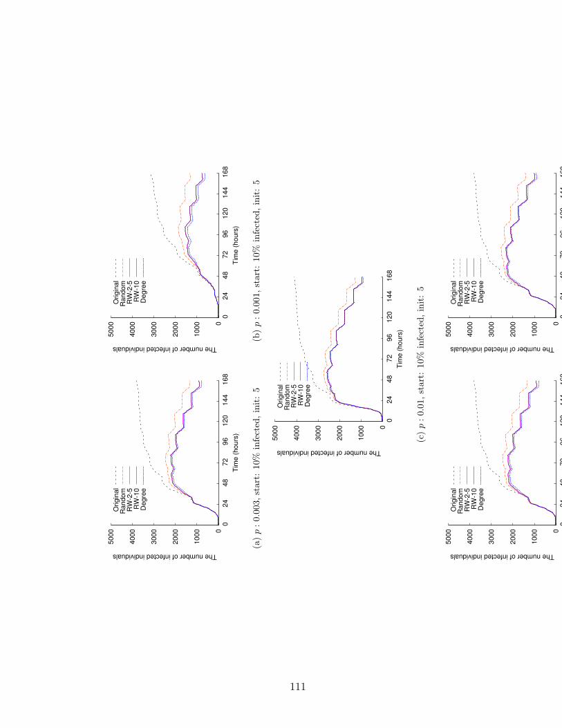
0

1000

2000

3000

4000

5000

0 2

4 4

8 7

2 9

6 1

20

144

168

The number of infected individuals

Tim

e (

hours

)

Origin

al

Random

RW

-2-5

RW

-10

Degre

e

(a)

p:0.0

03,st

art

:10%

infe

cted

,in

it:

5

0

1000

2000

3000

4000

5000

0 2

4 4

8 7

2 9

6 1

20

144

168


Tim

e (

hours

)

Origin

al

Random

RW

-2-5

RW

-10

Degre

e

(b)

p:0.0

01,st

art

:10%

infe

cted

,in

it:

5

0

1000

2000

3000

4000

5000

0 2

4 4

8 7

2 9

6 1

20

144

168


Tim

e (

hours

)

Origin

al

Random

RW

-2-5

RW

-10

Degre

e

(c)

p:0.0

1,st

art

:10%

infe

cted

,in

it:

5

0

1000

2000

3000

4000

5000

0 2

4 4

8 7

2 9

6 1

20

144

168


Origin

al

Random

RW

-2-5

RW

-10

Degre

e

0

1000

2000

3000

4000

5000

0 2

4 4

8 7

2 9

6 1

20

144

168


Origin

al

Random

RW

-2-5

RW

-10

Degre

e

111

In Figure 5.5, Original plots the curves without immunization as the baseline.

As we can see from these subfigures, the number of infected individuals increases

much more slowly from the midnight till the morning, compared with other periods

in a day, mainly because college students move less frequently during that time

period. It is true especially for the first 2 or 3 days, when a large number of students

get infected. In all figures of this chapter, RW-n plots the curves for generating a

single random-walk probe message from a given mobile device with n steps, and

RW-m-n for generating m probe messages from a mobile device with n steps.

In these 6 subfigures, Figures 5.5a, 5.5b, and 5.5c plot the number of infected

individuals with different infection probabilities, 0.003, 0.001 and 0.01, 5 initial in-

fections and immunizations after 10% of students are infected. Figures 5.5d and 5.5e

plot the cases for immunizations after 24 hours and 30% of infections with 0.003

infection probability and 5 initial infections. Figure 5.5f plots the case with 0.003

infection probability, 10 initial infections and immunizations after 10% infections.

As we can see from these 6 subfigures, RW-10 performs very close to Degree and

they all outperform Random. Compared to Random, the improvement of RW-10 ranges

from 14.10% (Figure 5.5c) to 25.36% (Figure 5.5b). On average RW-2-5 generates

the same amount of random-walk probe messages as RW-10, and it performs very

close to (slightly worse than) RW-10 because probe messages with longer steps have

more chances to visit influential users.

112

5.5.2.3 Effects of Various Random-Walk Parameters

We also evaluate the performance of random-walk based immunization with

different lengths, probabilities and frequencies of random walks performed by probe

messages, and plot the simulation results in Figures 5.6a, 5.6b and 5.6c. All the

curves in Figure 5.6 show the number of infected individuals under random-walk

based immunization with 0.001 infection probability, 5 initial infections and im-

munizations after 10% infections. As we can see from these 3 subfigures, we can

improve the performance of random-walk based immunization when increasing the

length of random walks from 1 to 10, increasing the probability from 0.1 to 0.4, or

increasing the frequency from once every 12 hours to 3 hours. However, we achieve

these improvements at the expense of higher message overhead.

We plot the control message overhead of iWander with different lengths, prob-

abilities and frequencies of random walks in Figures 5.7a, 5.7b and 5.7c. There

are three types of control messages, probe request and probe response messages for

device discovery, and random-walk probe messages for iWander. In all these subfig-

ures, the baseline is iWander with 1-step random walks and mobile devices generate

random-walk messages with probability 0.1 every 12 hours.

We plot the CDF of the amount of one-day per-user control messages transmit-

ted by mobile devices on 2004-03-01. As we can see from these subfigures, around

50% of mobile devices generate less than 200 control messages when using iWander.

For Degree, all messages are transmitted during device discovery and the number

of per-user control messages ranges from 1,441 to 25,608 for the simulated period.

113

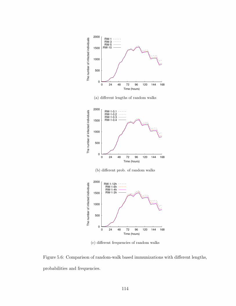
0

500

1000

1500

2000

0 24 48 72 96 120 144 168

The n

um

ber

of in

fecte

d indiv

iduals

Time (hours)

RW-1RW-3RW-5

RW-10

(a) different lengths of random walks

0

500

1000

1500

2000

0 24 48 72 96 120 144 168

The n

um

ber

of in

fecte

d indiv

iduals

Time (hours)

RW-1-0.1RW-1-0.2RW-1-0.3RW-1-0.4

(b) different prob. of random walks

0

500

1000

1500

2000

0 24 48 72 96 120 144 168

The n

um

ber

of in

fecte

d indiv

iduals

Time (hours)

RW-1-12hRW-1-6hRW-1-4hRW-1-3h

(c) different frequencies of random walks

Figure 5.6: Comparison of random-walk based immunizations with different lengths,

probabilities and frequencies.

114

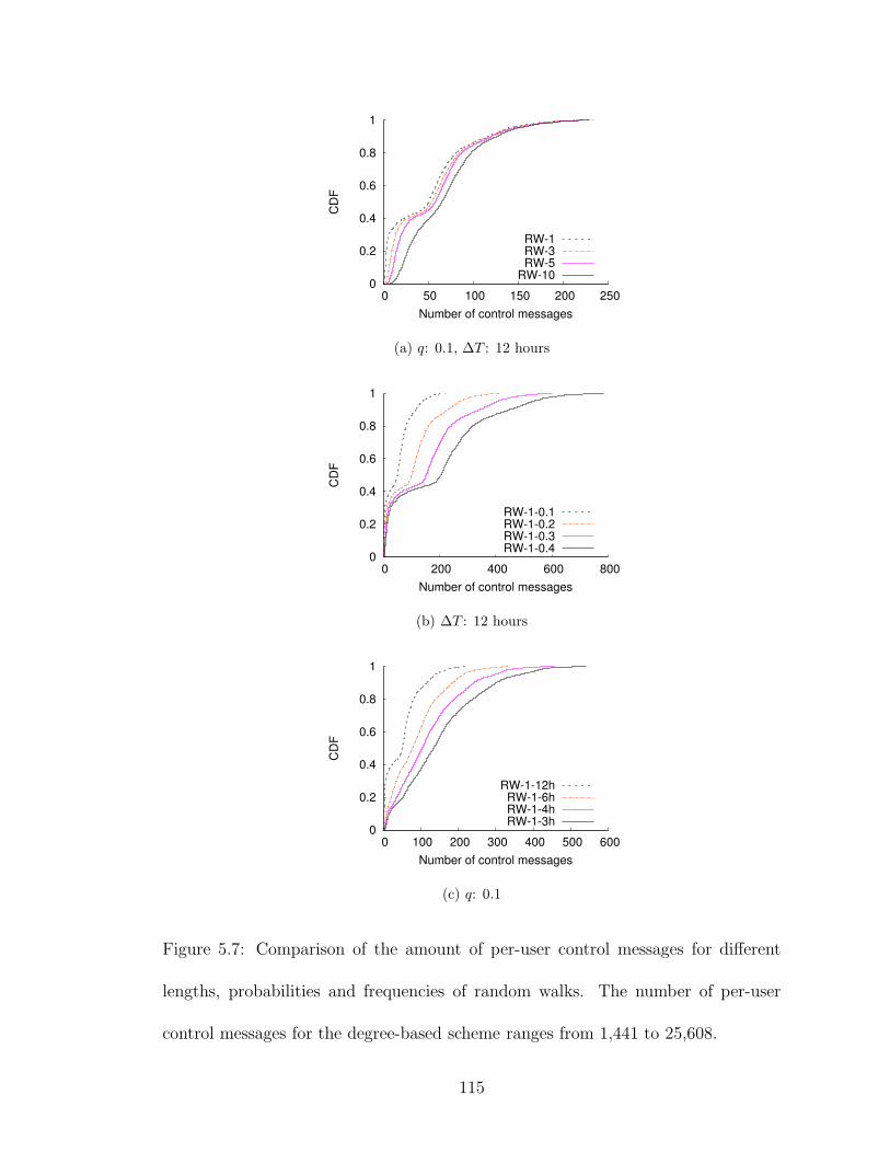
0

0.2

0.4

0.6

0.8

1

0 50 100 150 200 250

CD

F

Number of control messages

RW-1RW-3RW-5

RW-10

(a) q: 0.1, ∆T : 12 hours

0

0.2

0.4

0.6

0.8

1

0 200 400 600 800

CD

F


RW-1-0.1RW-1-0.2RW-1-0.3RW-1-0.4

(b) ∆T : 12 hours

0

0.2

0.4

0.6

0.8

1

0 100 200 300 400 500 600

CD

F


RW-1-12hRW-1-6hRW-1-4hRW-1-3h

(c) q: 0.1

Figure 5.7: Comparison of the amount of per-user control messages for different

lengths, probabilities and frequencies of random walks. The number of per-user

control messages for the degree-based scheme ranges from 1,441 to 25,608.

115

The amount of one-day per-user control messages transmitted by iWander is ex-

tremely low, less than 800 for all cases. An interesting observation from these three

subfigures is that there are two kinds of mobile devices: active (high mobility and

transmitting a large number of control messages) and inactive. In Section 5.4, we

harness this observation to improve the performance of mobile information dissem-

ination.

5.5.2.4 Early Detection of Outbreaks

We can also benefit from iWander for early outbreak detection, which is im-

portant to control the spread of infectious diseases [15, 24]. We investigate how

to choose a subset of students whose health conditions are monitored to provide

early detection, similar to the approach in Christakis and Fowler [15]. Motivated

by the observation that monitoring a sample of individuals with high centrality in

social-contact networks could allow early detection of contagious outbreaks before

they happen in the whole population [15], we propose to choose monitors based on

the random-walk counters maintained by iWander.

We plot the evolution of the number of infected monitors chosen randomly and

based on iWander in Figures 5.8a, 5.8b and 5.8c with 100, 200, and 400 monitors.

In this scenario, the infection probability is 0.003 and there are 5 initial infections.

Mobile devices generate random-walk probe messages with probability 0.1 every

hour. The medical staff choose a group of monitors based on the random-walk

counters reported at the noon of 2004-03-01. These subfigures confirm that iWander

116

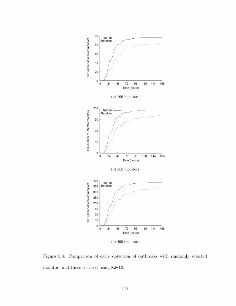
0

20

40

60

80

100

0 24 48 72 96 120 144 168

The n

um

ber

of in

fecte

d m

onitors

Time (hours)

RW-10Random

(a) 100 monitors

0

50

100

150

200

0 24 48 72 96 120 144 168

The n

um

ber

of in

fecte

d m

onitors

Time (hours)

RW-10Random

(b) 200 monitors

0

50

100

150

200

250

300

350

400

0 24 48 72 96 120 144 168

The n

um

ber

of in

fecte

d m

onitors

Time (hours)

RW-10Random

(c) 400 monitors

Figure 5.8: Comparison of early detection of outbreaks with randomly selected

monitors and those selected using RW-10.

117

does offer early outbreak detection, compared with the random selection scheme.

For example, if we draw the conclusion that an outbreak is occurring when 60% of

the monitors are infected, we can detect the outbreak around 21 hours earlier.

118

Chapter 6

Conclusions and Future Work

6.1 What We Have Done

In this dissertation, we investigate the problem of how to improve the effi-

ciency of hybrid mobile content delivery systems. We propose to send the delivered

content first to a small number of influential mobile users through wide-area cellular

communication. Then during the movement of these users, they will help forward

the content to others through local-area peer-to-peer communication. Previous work

on wide-area hybrid unicast/multicast considered mainly channel quality informa-

tion [56] and interference between local communications [11] when selecting the

relay devices. We advance the state of the art by taking the centrality information

of mobile users into account when identifying the initial target users.

Centrality estimation of mobile users is difficult due to two reasons. First, pre-

vious work on finding important users of information diffusion focuses on traditional

social networks with static relationship graphs [14, 45]. The contact graph of mo-

bile social networks changes dynamically because of the mobility of users. Second,

mobile devices are energy-constrained. Existing schemes that require the complete

social-contact graph of mobile users are not energy efficient due to frequent updates

of contact information between users.

We design both centralized and distributed schemes for the initial target-set

119

selection problem in mobile content delivery. Given the submodularity nature of

information dissemination functions that we prove for dynamic graphs, the greedy

algorithm can achieve a (1−1/e) approximation ratio. Differently from the greedy al-

gorithm that requires future mobility information, the heuristic algorithm leverages

the regularity of human mobility and uses history mobility information for future

content delivery. To reduce the communication overhead of centralized schemes, we

propose a lightweight and distributed protocol to identify influential mobile users

through random-walk sampling. This protocol uses probe messages that perform

fixed-length random walks to sample mobile users and estimates the centrality of

individuals based on the number of times their mobile devices are visited by these

probe messages. We prove that for expander-like static graphs the proposed random-

walk sampling is very close to sampling vertices according to their degrees. We verify

the effectiveness of our proposed approaches through extensive simulation studies

using both synthetic and real-world mobility traces.

6.2 Unaddressed Issues

In this section, we discuss several unsolved issues that we must take into

consideration for the large-scale deployment of our proposed approaches in mobile

content delivery systems.

The integration of effective incentive schemes into mobile content delivery is a

challenging problem. For content providers, with the hybrid delivery solution they

can decrease the amount of consumed cellular traffic and thus reduce their operation

120

cost. As a result, they may reduce the subscription fee for the initial target users.

To encourage social participation of mobile users, content providers can also exploit

other incentives: see, e.g., the Coupons approach of Garyfalos and Almeroth [29].

This system appends a sorted list of user IDs to a propagated message, which records

the sequence of users who helped to forward the content. Recently, Misra et al. [61]

propose a solution that provides incentives for peer-assisted services. Their goal is

to develop an economic framework that creates the right incentives for both users

and providers. They exploit a cooperative game theory approach to determine the

ideal incentive structure through fluid Shapley value. Similarly, we may apply this

scheme into the hybrid content delivery systems to encourage user participation.

Energy consumption is another important issue for the deployment of mobile

applications. In our current implementation of random-walk sampling, we use fixed

parameters for Bluetooth device discovery (e.g., inquiry duration and interval, and

inquiry scan window and interval). We believe that dynamically changing these

parameters according to user mobility patterns may make the device discovery pro-

cedure more energy efficient. For example, when users are not moving, larger inquiry

interval may be a better choice. Since device discovery is a common component for

several mobile applications like Social Serendipity [20] and Media Sharing [57], its

energy consumption can also be amortized by them. For data transfer after device

discovery, we can replace Bluetooth with WiFi to save battery life.

121

6.3 Future Directions

Several interesting future research problems arise naturally from this disserta-

tion work. The amount of cellular traffic will first decrease and then increase when

we add more users into the initial target set. Thus we need to find the optimal size

of a target set, given the budget of content providers. Another open problem related

to our proposed random-walk sampling is the theoretical analysis of discrete-time

random walks on dynamic graphs. Although a recent work of Figueiredo et al. [27]

has investigated the steady state distribution of continuous-time random walks on

dynamic graphs, our random walks are discrete in nature due to the non-continuous

device discovery.

When estimating the centrality of mobile users, we have not considered the

community structure [67] and temporal reachability [87] of the underlying social-

contact graphs and their interaction [74]. A future direction is to design a generic

framework that integrates several different metrics, including random-walk between-

ness, channel quality, community structure and temporal nature of social contacts.

For example, we can develop a new metric that combines the random-walk counter

and the community counter to improve the accuracy of centrality estimation. The

community counter records how many communities a mobile user belongs to and

users with a high community counter will be responsible for content forwarding [67].

Although the exchange of random-walk probe messages integrates implicitly the

temporal nature of social contacts, a deeper understanding of this property may

further improve the performance of content dissemination through local opportunis-

122

tic communications, as shown in Pietilainen and Diot [74] and Whitbeck et al. [87].

In this dissertation work, we have focused on leveraging local communica-

tions to enhance wide-area mobile content delivery. A natural extension would be

the investigation of more performance issues in the wide-area cellular networks.

Recently, we have seen several proposals about the “small cell” cellular network

architecture [13, 40], i.e., augmenting the existing macrocells with femtocells and

WiFi cells. However, there are a number of technical challenges in this small-cell

architecture, such as self-configuration, -optimization, and -healing mechanisms, in-

terference management, coverage and performance prediction, mobility management

and security. Further improving the efficiency of mobile content delivery by consid-

ering the architecture of cellular networks will be another interesting line of future

work.

123

Bibliography

[1] 3GPP-TS-22.246. Multimedia Broadcast/Multicast Service (MBMS) User Ser-vices, Mar. 2011.

[2] 3GPP2-C.S0054-A. CDMA2000 High Rate Broadcast-Multicast Packet DataAir Interface Specification, Feb. 2006.

[3] I. S. 802.11TM

2007. IEEE Standard for Information technology–Telecommunications and information exchange between systems–Local andmetropolitan area networks–Specific requirements–Part 11: Wireless LANMedium Access Control (MAC) and Physical Layer (PHY) Specifications, June2007.

[4] D. Aguayo, J. Bicket, S. Biswas, G. Judd, and R. Morris. Link-level Measure-ments from an 802.11b Mesh Network. In Proceedings of SIGCOMM 2004,pages 121–132, Aug.-Sept. 2004.

[5] H. Balakrishnan, S. Seshan, E. Amir, and R. H. Katz. Improving TCP/IPPerformance over Wireless Networks. In Proceedings of MOBICOM 1995, pages2–11, Nov. 1995.

[6] N. Balasubramanian, A. Balasubramanian, and A. Venkataramani. EnergyConsumption in Mobile Phones: A Measurement Study and Implications forNetwork Applications. In Proceedings of IMC 2009, pages 280–293, Nov. 2009.

[7] S. Banerjee, B. Bhattacharjee, and C. Kommareddy. Scalable Application LayerMulticast. In Proceedings of SIGCOMM 2002, pages 205–217, Aug. 2002.

[8] C. L. Barrett, S. J. Eidenbenz, L. Kroc, M. Marathe, and J. P. Smith. Para-metric Probabilistic Routing in Sensor Networks. Mobile Networks and Appli-cations, 10(4):529–544, Aug. 2005.

[9] A. Beach, M. Gartrell, S. Akkala, J. Elston, J. Kelley, K. Nishimoto, B. Ray,S. Razgulin, K. Sundaresan, B. Surendar, M. Terada, and R. Han. WhozThat?Evolving an Ecosystem for Context-Aware Mobile Social Networks. IEEE Net-work, 22(4):50–55, July-Aug. 2008.

[10] R. Beckman, K. Channakeshava, F. Huang, V. S. A. Kumar, A. Marathe,M. V. Marathe, and G. Pei. Implications of Dynamic Spectrum Access on theEfficiency of Primary Wireless Market. In Proceedings of DySPAN 2010, pages1–12, Apr. 2010.

[11] R. Bhatia, L. E. Li, H. Luo, and R. Ramjee. ICAM: Integrated Cellular andAd Hoc Multicast. IEEE Transactions on Mobile Computing, 5(8):1004–1015,Aug. 2006.

124

[12] A. Chaintreau, P. Hui, J. Crowcroft, C. Diot, R. Gass, and J. Scott. Impact ofHuman Mobility on Opportunistic Forwarding Algorithms. IEEE Transactionson Mobile Computing, 6(6):606–620, June 2007.

[13] V. Chandrasekhar, J. G. Andrews, and A. Gatherer. Femtocell Networks: ASurvey. IEEE Communications Magazine, 46(9):59–67, Sept. 2008.

[14] W. Chen, Y. Wang, and S. Yang. Efficient Influence Maximization in SocialNetworks. In Proceedings of SIGKDD 2009, pages 199–207, June-July 2009.

[15] N. A. Christakis and J. H. Fowler. Social Network Sensors for Early Detectionof Contagious Outbreaks. PLoS ONE, 5(9):e12948, Sept. 2010.

[16] R. M. Christley, G. L. Pinchbeck, R. G. Bowers, D. Clancy, N. P. French,R. Bennett, and J. Turner. Infection in Social Networks: Using NetworkAnalysis to Identify High-Risk Individuals. American Journal of Epidemiol-ogy, 162(10):1024–1031, Nov. 2005.

[17] Y.-H. Chu, S. G. Rao, and H. Zhang. A Case for End System Multicast. InProceedings of SIGMETRICS 2000, pages 1–12, June 2000.

[18] E. W. Dijkstra and C. S. Scholten. Termination Detection for Diffusing Com-putations. Information Processing Letters, 11(1):1–4, Aug. 1980.

[19] P. Domingos and M. Richardson. Mining the Network Value of Customers. InProceedings of SIGKDD 2001, pages 57–66, Aug. 2001.

[20] N. Eagle and A. Pentland. Social Serendipity: Mobilizing Social Software.IEEE Pervasive Computing, 4(2):28–34, Apr.-June 2005.

[21] N. Eagle, A. S. Pentland, and D. Lazer. Inferring friendship network structureby using mobile phone data. Proceedings of the National Academy of Sciences,106(36):15274–15278, Sept. 2009.

[22] D. Eckhardt and P. Steenkiste. Measurement and Analysis of the Error Char-acteristics of an In-Building Wireless Network. In Proceedings of SIGCOMM1996, pages 243–254, Aug. 1996.

[23] E. O. Elliot. Estimates of Error Rates for Codes on Burst-Noise Channels. BellSystems Technical Journal, 42:1977–1997, Sept. 1963.

[24] S. Eubank, H. Guclu, V. S. A. Kumar, M. V. Marathe, A. Srinivasan,Z. Toroczkai, and N. Wang. Modelling Disease Outbreaks in Realistic UrbanSocial Networks. Nature, 429(6988):180–184, May 2004.

[25] S. Eubank, V. A. Kumar, M. V. Marathe, A. Srinivasan, and N. Wang. Struc-tural and Algorithmic Aspects of Massive Social Networks. In Proceedings ofSODA 2004, pages 718–727, Jan. 2004.

125

[26] S. L. Feld. Why Your Friends Have More Friends Than You Do. AmericanJournal of Sociology, 96(6):1464–1477, May 1991.

[27] D. Figueiredo, P. Nain, B. Ribeiro, E. de Souza e Silva, and D. Towsley. Char-acterizing Continuous Time Random Walks on Time Varying Graphs. In Pro-ceedings of SIGMETRICS 2012, pages 307–318, June 2012.

[28] S. Gaonkar, J. Li, R. R. Choudhury, L. Cox, and A. Schmidt. Micro-Blog: Shar-ing and Querying Content Through Mobile Phones and Social Participation.In Proceedings of MobiSys 2008, pages 174–186, June 2008.

[29] A. Garyfalos and K. C. Almeroth. Coupons: A Multilevel Incentive Scheme forInformation Dissemination in Mobile Networks. IEEE Transactions on MobileComputing, 7(6):792–804, June 2008.

[30] E. N. Gilbert. Capacity of a Burst-Noise Channel. Bell Systems TechnicalJournal, 39:1253–1265, Sept. 1960.

[31] M. Gjoka, M. Kurant, C. T. Butts, and A. Markopoulou. Walking in Facebook:A Case Study of Unbiased Sampling of OSNs. In Proceedings of INFOCOM2010, pages 1–9, Mar. 2010.

[32] M. X. Goemans, L. E. Li, V. S. Mirrokni, and M. Thottan. Market SharingGames Applied to Content Distribution in Ad-Hoc Networks. In Proceedingsof MOBIHOC 2004, pages 55–66, May 2004.

[33] J. Goldenberg, B. Libai, and E. Muller. Talk of the Network: A ComplexSystems Look at the Underlying Process of Word-of-Mouth. Marketing Letters,12(3):211–223, Aug. 2001.

[34] M. C. Gonzalez, C. A. Hidalgo, and A.-L. Barabasi. Understanding individualhuman mobility patterns. Nature, 453(7196):779–782, June 2008.

[35] F. Gringoli and L. Nava. Open FirmWare for WiFi networks. http://www.

ing.unibs.it/openfwwf/.

[36] M. Grossglauser and D. N. C. Tse. Mobility Increases the Capacity of Ad HocWireless Networks. IEEE/ACM Transactions on Networking, 10(4):477–486,Aug. 2002.

[37] D. Halperin, W. Hu, A. Sheth, and D. Wetherall. Predictable 802.11 PacketDelivery from Wireless Channel Measurements. In Proceedings of SIGCOMM2010, pages 159–170, Aug.-Sept. 2010.

[38] B. Han, P. Hui, V. S. A. Kumar, M. V. Marathe, J. Shao, and A. Srini-vasan. Mobile Data Offloading through Opportunistic Communications andSocial Participation. IEEE Transactions on Mobile Computing, 11(5):821–834,May 2012.

126

[39] B. Hoppe and Eva Tardos. The Quickest Transshipment Problem. In Proceed-ings of SODA 1995, pages 512–521, Jan. 1995.

[40] J. Hoydis, M. Kobayashi, and M. Debbah. Green Small-Cell Networks. IEEEVehicular Technology Magazine, 6(1):37–43, Mar. 2011.

[41] C. Intanagonwiwat, R. Govindan, D. Estrin, J. Heidemann, and F. Silva. Di-rected Diffusion for Wireless Sensor Networking. IEEE/ACM Transactions onNetworking, 11(1):2–16, Feb. 2003.

[42] S. Ioannidis, A. Chaintreau, and L. Massoulie. Optimal and Scalable Distri-bution of Content Updates over a Mobile Social Network. In Proceedings ofINFOCOM 2009, pages 1422–1430, Apr. 2009.

[43] K. Jamieson and H. Balakrishnan. PPR: Partial Packet Recovery for WirelessNetworks. In Proceedings of SIGCOMM 2007, pages 409–420, Aug. 2007.

[44] S. Katti, H. Rahul, W. Hu, D. Katabi, M. Medard, and J. Crowcroft. XORsin The Air: Practical Wireless Network Coding. In Proceedings of SIGCOMM2006, pages 243–254, Sept. 2006.

[45] D. Kempe, J. Kleinberg, and Eva Tardos. Maximizing the Spread of Influencethrough a Social Network. In Proceedings of SIGKDD 2003, pages 137–146,Aug. 2003.

[46] W. O. Kermack and A. G. McKendrick. A Contribution to the MathematicalTheory of Epidemics. Proceedings of the Royal Society of London (Series A),115(772):700–721, Aug. 1927.

[47] A. Kopke, A. Willig, and H. Karl. Chaotic Maps as Parsimonious Bit ErrorModels of Wireless Channels. In Proceedings of the 22nd Annual Joint Confer-ence of the IEEE Computer and Communications Societies (INFOCOM 2003),pages 513–523, Mar.-Apr. 2003.

[48] V. Kostakos. Temporal Graphs. Physica A: Statistical Mechanics and its Ap-plications, 388(6):1007–1023, Mar. 2009.

[49] D. Kotz, T. Henderson, I. Abyzov, and J. Yeo. CRAWDAD tracedartmouth/campus/movement/01 04 (v. 2005-03-08). Downloaded fromhttp://crawdad.cs.dartmouth.edu/dartmouth/campus/movement/01_04,Mar. 2005.

[50] U. C. Kozat. On the Throughput Capacity of Opportunistic Multicasting withErasure Codes. In Proceedings of INFOCOM 2008, pages 520–528, Apr. 2008.

[51] J. Leskovec, J. Kleinberg, and C. Faloutsos. Graphs over Time: Densifica-tion Laws, Shrinking Diameters and Possible Explanations. In Proceedings ofSIGKDD 2005, pages 177–187, Aug. 2005.

127

[52] L. E. Li, K. Tan, H. Viswanathan, Y. Xu, and Y. R. Yang. Retransmission 6=Repeat: Simple Retransmission Permutation Can Resolve Overlapping ChannelCollisions. In Proceedings of MOBICOM 2010, pages 281–292, Sept. 2010.

[53] K. C.-J. Lin, N. Kushman, and D. Katabi. ZipTx: Harnessing Partial Packetsin 802.11 Networks. In Proceedings of MOBICOM 2008, pages 351–362, Sept.2008.

[54] C. Lindemann and O. P. Waldhorst. Modeling Epidemic Information Dissemi-nation on Mobile Devices with Finite Buffers. In Proceedings of SIGMETRICS2005, pages 121–132, June 2005.

[55] L. Lovasz. Random Walks on Graphs: A Survey. Combinatorics, Paul Erdosis Eighty, 2(1):1–46, 1993.

[56] H. Luo, R. Ramjee, P. Sinha, L. E. Li, and S. Lu. UCAN: A Unified Cellularand Ad-Hoc Network Architecture. In Proceedings of MOBICOM 2003, pages353–367, Sept. 2003.

[57] L. McNamara, C. Mascolo, and L. Capra. Media Sharing based on ColocationPrediction in Urban Transport. In Proceedings of MOBICOM 2008, pages 58–69, Sept. 2008.

[58] A. Mei and J. Stefa. SWIM: A Simple Model to Generate Small Mobile Worlds.In Proceedings of INFOCOM 2009, pages 2106–2113, Apr. 2009.

[59] E. Miluzzo, N. D. Lane, K. Fodor, R. Peterson, H. Lu, M. Musolesi, S. B. Eisen-man, X. Zheng, and A. T. Campbell. Sensing Meets Mobile Social Networks:The Design, Implementation and Evaluation of the CenceMe Application. InProceedings of SenSys 2008, pages 337–350, Nov. 2008.

[60] A. Mishra, S. Rayanchu, D. Agrawal, and S. Banerjee. Supporting ContinuousMobility through Multi-rate Wireless Packetization. In Proceedings of HotMo-bile 2008, pages 33–37, Feb. 2008.

[61] V. Misra, S. Ioannidis, A. Chaintreau, and L. Massoulie. Incentivizing Peer-Assisted Services: A Fluid Shapley Value Approach. In Proceedings of SIG-METRICS 2010, pages 215–226, June 2010.

[62] A. Miu, H. Balakrishnan, and C. E. Koksal. Improving Loss Resilience withMulti-Radio Diversity in Wireless Networks. In Proceedings of MOBICOM2005, pages 16–30, Aug.-Sept. 2005.

[63] P. H. Moose. A Technique for Orthogonal Frequency Division Multiplex-ing Frequency Offset Correction. IEEE Transactions on Communications,42(10):2908–2914, Oct. 1994.

128

[64] M. Motani, V. Srinivasan, and P. S. Nuggehalli. PeopleNet: Engineering AWireless Virtual Social Network. In Proceedings of MOBICOM 2005, pages243–257, Aug.-Sept. 2005.

[65] G. L. Nemhauser, L. A. Wolsey, and M. L. Fisher. An analysis of approxima-tions for maximizing submodular set functions. Mathematical Programming,14(1):265–294, Dec. 1978.

[66] M. E. Newman. A measure of betweenness centrality based on random walks.Social Networks, 27(1):39–54, Jan. 2005.

[67] N. P. Nguyen, T. N. Dinh, S. Tokala, and M. T. Thai. Overlapping Communitiesin Dynamic Networks: Their Detection and Mobile Applications. In Proceedingsof MOBICOM 2011, pages 85–95, Sept. 2011.

[68] J. D. Noh and H. Rieger. Random Walks on Complex Networks. PhysicalReview Letters, 92(11):118701, Mar. 2004.

[69] C. Oberli. ML-based Tracking Algorithms for MIMO-OFDM. IEEE Transac-tions on Wireless Communications, 6(7):2630–2639, July 2007.

[70] L. Page, S. Brin, R. Motwani, and T. Winograd. The PageRank CitationRanking: Bringing Order to the Web. Technical Report 1999-66, Nov. 1999.

[71] M. Papadopouli and H. Schulzrinne. Effects of Power Conservation, WirelessCoverage and Cooperation on Data Dissemination among Mobile Devices. InProceedings of MOBIHOC 2001, pages 117–127, Oct. 2001.

[72] B. Pasztor, L. Mottola, C. Mascolo, G. P. Picco, S. Ellwood, and D. Mac-donald. Selective Reprogramming of Mobile Sensor Networks through SocialCommunity Detection. In Proceedings of EWSN 2010, pages 178–193, Feb.2010.

[73] K. Pearson. The Problem of the Random Walk. Nature, 72(1865):294, July1905.

[74] A.-K. Pietilainen and C. Diot. Dissemination in Opportunistic Social Networks:the Role of Temporal Communities. In Proceedings of MOBIHOC 2012, pages165–174, June 2012.

[75] J. Pollak, G. Gay, S. Byrne, E. Wagner, D. Retelny, and L. Humphreys. It’sTime to Eat! Using Mobile Games to Promote Healthy Eating. IEEE PervasiveComputing, 9(3):21–27, July-Sept. 2010.

[76] L. Qiu, Y. Zhang, F. Wang, M. K. Han, and R. Mahajan. A General Modelof Wireless Interference. In Proceedings of MOBICOM 2007, pages 171–182,Sept. 2007.

129

[77] C. Reis, R. Mahajan, M. Rodrig, D. Wetherall, and J. Zahorjan. Measurement-Based Models of Delivery and Interference in Static Wireless Networks. InProceedings of SIGCOMM 2006, pages 51–62, Sept. 2006.

[78] B. Ribeiro and D. Towsley. Estimating and Sampling Graphs with Multidi-mensional Random Walks. In Proceedings of IMC 2010, pages 390–403, Nov.2010.

[79] M. Richardson and P. Domingos. Mining Knowledge-Sharing Sites for ViralMarketing. In Proceedings of SIGKDD 2002, pages 61–70, July 2002.

[80] P. S. Sindhu. Retransmission Error Control with Memory. IEEE Transactionson Communications, 25(5):473–479, May 1977.

[81] M. Speth, S. A. Fechtel, G. Fock, and H. Meyr. Optimum Receiver Design forWireless Broad-Band Systems Using OFDM – Part I. IEEE Transactions onCommunications, 47(11):1668–1677, Nov. 1999.

[82] D. Stutzbach, R. Rejaie, N. Dufld, S. Sen, and W. Willinger. On UnbiasedSampling for Unstructured Peer-to-Peer Networks. In Proceedings of IMC 2006,pages 27–39, Oct. 2006.

[83] D. Tse and P. Viswanath. Fundamentals of Wireless Communication. Cam-bridge University Press, 2005.

[84] T. W. Valente. Network Models of the Diffusion of Innovations. HamptonPress, 1995.

[85] V. Vukadinovic and G. Karlsson. Spectral Efficiency of Mobility-Assisted Pod-casting in Cellular Networks. In Proceedings of MobiOpp 2010, pages 51–57,Feb. 2010.

[86] D. J. Watts and S. H. Strogatz. Collective dynamics of ‘small-world’ networks.Nature, 393(6684):440–442, June 1998.

[87] J. Whitbeck, M. D. de Amorim, V. Conan, and J.-L. Guillaume. TemporalReachability Graphs. In Proceedings of MOBICOM 2012, Aug. 2012.

[88] A. Willig, M. Kubisch, C. Hoene, and A. Wolisz. Measurements of a WirelessLink in an Industrial Environment Using an IEEE 802.11-Compliant PhysicalLayer. IEEE Transactions on Industrial Electronics, 49(6):1265–1282, Dec.2002.

[89] H. Won, H. Cai, D. Y. Eun, K. Guo, A. Netravali, I. Rhee, and K. Sabnani.Multicast Scheduling in Cellular Data Networks. In Proceedings of INFOCOM2007, pages 1172–1180, May 2007.

[90] G. Woo, P. Kheradpour, D. Shen, and D. Katabi. Beyond the Bits: Coop-erative Packet Recovery Using Physical Layer Information. In Proceedings ofMOBICOM 2007, pages 147–158, Sept. 2007.

130

[91] Y. Xie, V. Sekar, D. A. Maltz, M. K. Reiter, and H. Zhang. Worm OriginIdentification Using Random Moonwalks. In Proceedings of the 2005 IEEESymposium on Security and Privacy, pages 242–256, May 2005.

[92] H. Yu, M. Kaminsky, P. B. Gibbons, and A. Flaxman. SybilGuard: DefendingAgainst Sybil Attacks via Social Networks. In Proceedings of SIGCOMM 2006,pages 267–278, Sept. 2006.

[93] Z. Zhu, G. Cao, S. Zhu, S. Ranjan, and A. Nucci. A Social Network BasedPatching Scheme for Worm Containment in Cellular Networks. In Proceedingsof INFOCOM 2009, pages 1476–1484, Apr. 2009.

[94] M. Zorzi, R. R. Rao, and L. B. Milstein. Error Statistics in Data Transmissionover Fading Channels. IEEE Transactions on Communications, 46(11):1468–1477, Nov. 1998.

[95] G. Zyba, G. M. Voelker, S. Ioannidis, and C. Diot. Dissemination in Oppor-tunistic Mobile Ad-hoc Networks: the Power of the Crowd. In Proceedings ofINFOCOM 2011, pages 1179–1187, Apr. 2011.

131

abstract wide-area mobile content delivery bo han, doctor of

Documents