World Models

David Ha 1 Jurgen Schmidhuber 2 3

AbstractWe explore building generative neural networkmodels of popular reinforcement learningenvironments. Our world model can be trainedquickly in an unsupervised manner to learn acompressed spatial and temporal representationof the environment. By using features extractedfrom the world model as inputs to an agent, wecan train a very compact and simple policy thatcan solve the required task. We can even trainour agent entirely inside of its own hallucinateddream generated by its world model, and transferthis policy back into the actual environment.

An interactive version of this paper is available athttps://worldmodels.github.io

1. IntroductionHumans develop a mental model of the world based onwhat they are able to perceive with their limited senses. Thedecisions and actions we make are based on this internalmodel. Jay Wright Forrester, the father of system dynamics,described a mental model as:

The image of the world around us, which we carry in ourhead, is just a model. Nobody in his head imagines allthe world, government or country. He has only selectedconcepts, and relationships between them, and uses thoseto represent the real system. (Forrester, 1971)

To handle the vast amount of information that flows throughour daily lives, our brain learns an abstract representationof both spatial and temporal aspects of this information.We are able to observe a scene and remember an abstractdescription thereof (Cheang & Tsao, 2017; Quiroga et al.,2005). Evidence also suggests that what we perceive at anygiven moment is governed by our brain’s prediction of thefuture based on our internal model (Nortmann et al., 2015;Gerrit et al., 2013).

One way of understanding the predictive model inside of ourbrains is that it might not be about just predicting the futurein general, but predicting future sensory data given our

1Google Brain 2NNAISENSE 3Swiss AI Lab, IDSIA (USI & SUPSI)

Figure 1. A World Model, from Scott McCloud’s UnderstandingComics. (McCloud, 1993; E, 2012)

current motor actions (Keller et al., 2012; Leinweber et al.,2017). We are able to instinctively act on this predictivemodel and perform fast reflexive behaviours when we facedanger (Mobbs et al., 2015), without the need to consciouslyplan out a course of action.

Take baseball for example. A batter has milliseconds to de-cide how they should swing the bat – shorter than the timeit takes for visual signals to reach our brain. The reasonwe are able to hit a 100 mph fastball is due to our ability toinstinctively predict when and where the ball will go. Forprofessional players, this all happens subconsciously. Theirmuscles reflexively swing the bat at the right time and loca-tion in line with their internal models’ predictions (Gerritet al., 2013). They can quickly act on their predictions ofthe future without the need to consciously roll out possiblefuture scenarios to form a plan (Hirshon, 2013).

Figure 2. What we see is based on our brain’s prediction of thefuture (Kitaoka, 2002; Watanabe et al., 2018).

arX

iv:1

803.

1012

2v4

[cs

.LG

] 9

May

201

8

World Models

In many reinforcement learning (RL) problems (Kaelblinget al., 1996; Sutton & Barto, 1998; Wiering & van Otterlo,2012), an artificial agent also benefits from having a goodrepresentation of past and present states, and a good pre-dictive model of the future (Werbos, 1987; Silver, 2017),preferably a powerful predictive model implemented on ageneral purpose computer such as a recurrent neural network(RNN) (Schmidhuber, 1990a;b; 1991a).

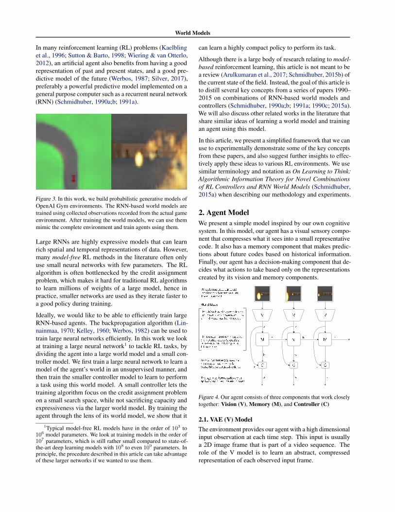
Figure 3. In this work, we build probabilistic generative models ofOpenAI Gym environments. The RNN-based world models aretrained using collected observations recorded from the actual gameenvironment. After training the world models, we can use themmimic the complete environment and train agents using them.

Large RNNs are highly expressive models that can learnrich spatial and temporal representations of data. However,many model-free RL methods in the literature often onlyuse small neural networks with few parameters. The RLalgorithm is often bottlenecked by the credit assignmentproblem, which makes it hard for traditional RL algorithmsto learn millions of weights of a large model, hence inpractice, smaller networks are used as they iterate faster toa good policy during training.

Ideally, we would like to be able to efficiently train largeRNN-based agents. The backpropagation algorithm (Lin-nainmaa, 1970; Kelley, 1960; Werbos, 1982) can be used totrain large neural networks efficiently. In this work we lookat training a large neural network1 to tackle RL tasks, bydividing the agent into a large world model and a small con-troller model. We first train a large neural network to learn amodel of the agent’s world in an unsupervised manner, andthen train the smaller controller model to learn to performa task using this world model. A small controller lets thetraining algorithm focus on the credit assignment problemon a small search space, while not sacrificing capacity andexpressiveness via the larger world model. By training theagent through the lens of its world model, we show that it

1Typical model-free RL models have in the order of 103 to106 model parameters. We look at training models in the order of107 parameters, which is still rather small compared to state-of-the-art deep learning models with 108 to even 109 parameters. Inprinciple, the procedure described in this article can take advantageof these larger networks if we wanted to use them.

can learn a highly compact policy to perform its task.

Although there is a large body of research relating to model-based reinforcement learning, this article is not meant to bea review (Arulkumaran et al., 2017; Schmidhuber, 2015b) ofthe current state of the field. Instead, the goal of this article isto distill several key concepts from a series of papers 1990–2015 on combinations of RNN-based world models andcontrollers (Schmidhuber, 1990a;b; 1991a; 1990c; 2015a).We will also discuss other related works in the literature thatshare similar ideas of learning a world model and trainingan agent using this model.

In this article, we present a simplified framework that we canuse to experimentally demonstrate some of the key conceptsfrom these papers, and also suggest further insights to effec-tively apply these ideas to various RL environments. We usesimilar terminology and notation as On Learning to Think:Algorithmic Information Theory for Novel Combinationsof RL Controllers and RNN World Models (Schmidhuber,2015a) when describing our methodology and experiments.

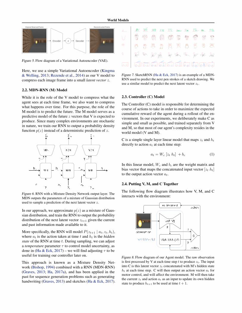
2. Agent ModelWe present a simple model inspired by our own cognitivesystem. In this model, our agent has a visual sensory compo-nent that compresses what it sees into a small representativecode. It also has a memory component that makes predic-tions about future codes based on historical information.Finally, our agent has a decision-making component that de-cides what actions to take based only on the representationscreated by its vision and memory components.

Figure 4. Our agent consists of three components that work closelytogether: Vision (V), Memory (M), and Controller (C)

2.1. VAE (V) ModelThe environment provides our agent with a high dimensionalinput observation at each time step. This input is usuallya 2D image frame that is part of a video sequence. Therole of the V model is to learn an abstract, compressedrepresentation of each observed input frame.

World Models

Encoder z Decoder

Original Observed Frame Reconstructed Frame

Figure 5. Flow diagram of a Variational Autoencoder (VAE).

Here, we use a simple Variational Autoencoder (Kingma& Welling, 2013; Rezende et al., 2014) as our V model tocompress each image frame into a small latent vector z.

2.2. MDN-RNN (M) Model

While it is the role of the V model to compress what theagent sees at each time frame, we also want to compresswhat happens over time. For this purpose, the role of theM model is to predict the future. The M model serves as apredictive model of the future z vectors that V is expected toproduce. Since many complex environments are stochasticin nature, we train our RNN to output a probability densityfunction p(z) instead of a deterministic prediction of z.

Figure 6. RNN with a Mixture Density Network output layer. TheMDN outputs the parameters of a mixture of Gaussian distributionused to sample a prediction of the next latent vector z.

In our approach, we approximate p(z) as a mixture of Gaus-sian distribution, and train the RNN to output the probabilitydistribution of the next latent vector zt+1 given the currentand past information made available to it.

More specifically, the RNN will model P (zt+1 | at, zt, ht),where at is the action taken at time t and ht is the hiddenstate of the RNN at time t. During sampling, we can adjusta temperature parameter τ to control model uncertainty, asdone in (Ha & Eck, 2017) – we will find adjusting τ to beuseful for training our controller later on.

This approach is known as a Mixture Density Net-work (Bishop, 1994) combined with a RNN (MDN-RNN)(Graves, 2013; Ha, 2017a), and has been applied in thepast for sequence generation problems such as generatinghandwriting (Graves, 2013) and sketches (Ha & Eck, 2017).

Figure 7. SketchRNN (Ha & Eck, 2017) is an example of a MDN-RNN used to predict the next pen strokes of a sketch drawing. Weuse a similar model to predict the next latent vector zt.

2.3. Controller (C) Model

The Controller (C) model is responsible for determining thecourse of actions to take in order to maximize the expectedcumulative reward of the agent during a rollout of the en-vironment. In our experiments, we deliberately make C assimple and small as possible, and trained separately from Vand M, so that most of our agent’s complexity resides in theworld model (V and M).

C is a simple single layer linear model that maps zt and htdirectly to action at at each time step:

at =Wc [zt ht] + bc (1)

In this linear model, Wc and bc are the weight matrix andbias vector that maps the concatenated input vector [zt ht]to the output action vector at.

2.4. Putting V, M, and C Together

The following flow diagram illustrates how V, M, and Cinteracts with the environment:

Figure 8. Flow diagram of our Agent model. The raw observationis first processed by V at each time step t to produce zt. The inputinto C is this latent vector zt concatenated with M’s hidden stateht at each time step. C will then output an action vector at formotor control, and will affect the environment. M will then takethe current zt and action at as an input to update its own hiddenstate to produce ht+1 to be used at time t+ 1.

World Models

Below is the pseudocode for how our agent model is usedin the OpenAI Gym (Brockman et al., 2016) environment:

def rollout(controller):’’’ env, rnn, vae are ’’’’’’ global variables ’’’obs = env.reset()h = rnn.initial_state()done = Falsecumulative_reward = 0while not done:

z = vae.encode(obs)a = controller.action([z, h])obs, reward, done = env.step(a)cumulative_reward += rewardh = rnn.forward([a, z, h])

return cumulative_reward

Running this function on a given controller C willreturn the cumulative reward during a rollout.

This minimal design for C also offers important practicalbenefits. Advances in deep learning provided us with thetools to train large, sophisticated models efficiently, pro-vided we can define a well-behaved, differentiable loss func-tion. Our V and M models are designed to be trained effi-ciently with the backpropagation algorithm using modernGPU accelerators, so we would like most of the model’scomplexity, and model parameters to reside in V and M.The number of parameters of C, a linear model, is mini-mal in comparison. This choice allows us to explore moreunconventional ways to train C – for example, even us-ing evolution strategies (ES) (Rechenberg, 1973; Schwefel,1977) to tackle more challenging RL tasks where the creditassignment problem is difficult.

To optimize the parameters of C, we chose the Covariance-Matrix Adaptation Evolution Strategy (CMA-ES) (Hansen,2016; Hansen & Ostermeier, 2001) as our optimizationalgorithm since it is known to work well for solution spacesof up to a few thousand parameters. We evolve parametersof C on a single machine with multiple CPU cores runningmultiple rollouts of the environment in parallel.

For more specific information about the models, training pro-cedures, and environments used in our experiments, pleaserefer to the Appendix section.

3. Car Racing ExperimentIn this section, we describe how we can train the Agentmodel described earlier to solve a car racing task. To ourknowledge, our agent is the first known solution to achievethe score required to solve this task.2

2We find this task interesting because although it is not difficultto train an agent to wobble around randomly generated tracks

3.1. World Model for Feature Extraction

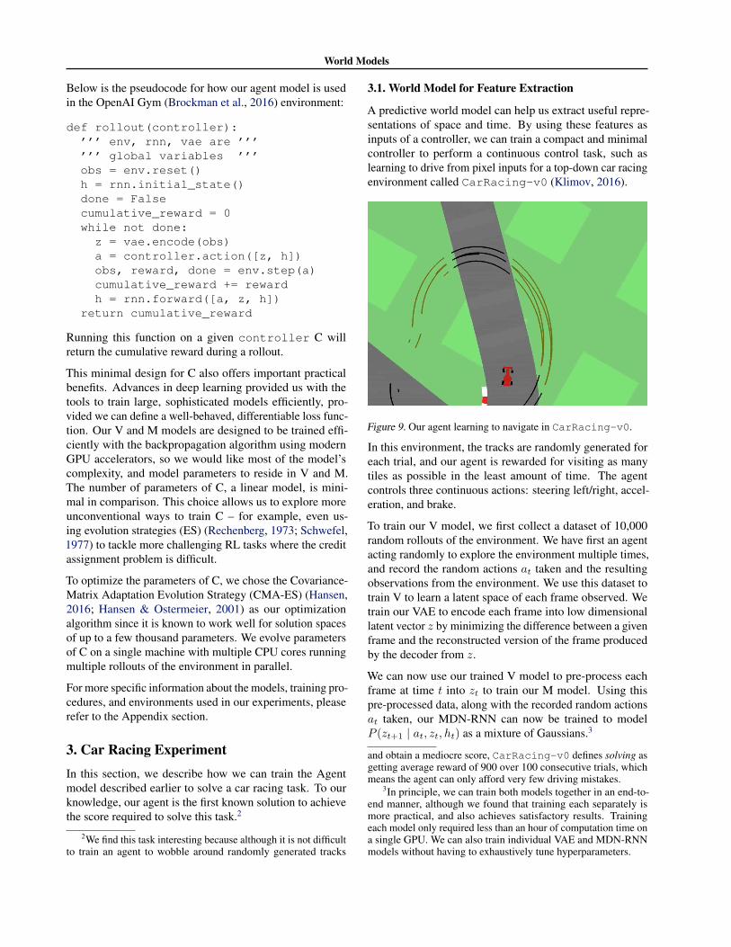
A predictive world model can help us extract useful repre-sentations of space and time. By using these features asinputs of a controller, we can train a compact and minimalcontroller to perform a continuous control task, such aslearning to drive from pixel inputs for a top-down car racingenvironment called CarRacing-v0 (Klimov, 2016).

Figure 9. Our agent learning to navigate in CarRacing-v0.

In this environment, the tracks are randomly generated foreach trial, and our agent is rewarded for visiting as manytiles as possible in the least amount of time. The agentcontrols three continuous actions: steering left/right, accel-eration, and brake.

To train our V model, we first collect a dataset of 10,000random rollouts of the environment. We have first an agentacting randomly to explore the environment multiple times,and record the random actions at taken and the resultingobservations from the environment. We use this dataset totrain V to learn a latent space of each frame observed. Wetrain our VAE to encode each frame into low dimensionallatent vector z by minimizing the difference between a givenframe and the reconstructed version of the frame producedby the decoder from z.

We can now use our trained V model to pre-process eachframe at time t into zt to train our M model. Using thispre-processed data, along with the recorded random actionsat taken, our MDN-RNN can now be trained to modelP (zt+1 | at, zt, ht) as a mixture of Gaussians.3

and obtain a mediocre score, CarRacing-v0 defines solving asgetting average reward of 900 over 100 consecutive trials, whichmeans the agent can only afford very few driving mistakes.

3In principle, we can train both models together in an end-to-end manner, although we found that training each separately ismore practical, and also achieves satisfactory results. Trainingeach model only required less than an hour of computation time ona single GPU. We can also train individual VAE and MDN-RNNmodels without having to exhaustively tune hyperparameters.

World Models

In this experiment, the world model (V and M) has no knowl-edge about the actual reward signals from the environment.Its task is simply to compress and predict the sequence ofimage frames observed. Only the Controller (C) Modelhas access to the reward information from the environment.Since there are a mere 867 parameters inside the linear con-troller model, evolutionary algorithms such as CMA-ES arewell suited for this optimization task.

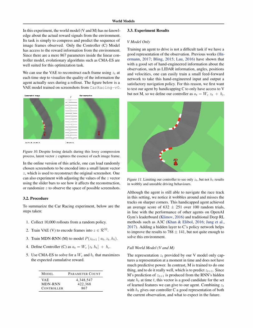
We can use the VAE to reconstruct each frame using zt ateach time step to visualize the quality of the information theagent actually sees during a rollout. The figure below is aVAE model trained on screenshots from CarRacing-v0.

Figure 10. Despite losing details during this lossy compressionprocess, latent vector z captures the essence of each image frame.

In the online version of this article, one can load randomlychosen screenshots to be encoded into a small latent vectorz, which is used to reconstruct the original screenshot. Onecan also experiment with adjusting the values of the z vectorusing the slider bars to see how it affects the reconstruction,or randomize z to observe the space of possible screenshots.

3.2. Procedure

To summarize the Car Racing experiment, below are thesteps taken:

1. Collect 10,000 rollouts from a random policy.

2. Train VAE (V) to encode frames into z ∈ R32.

3. Train MDN-RNN (M) to model P (zt+1 | at, zt, ht).

4. Define Controller (C) as at =Wc [zt ht] + bc.

5. Use CMA-ES to solve for a Wc and bc that maximizesthe expected cumulative reward.

MODEL PARAMETER COUNT

VAE 4,348,547MDN-RNN 422,368CONTROLLER 867

3.3. Experiment Results

V Model Only

Training an agent to drive is not a difficult task if we have agood representation of the observation. Previous works (Hn-ermann, 2017; Bling, 2015; Lau, 2016) have shown thatwith a good set of hand-engineered information about theobservation, such as LIDAR information, angles, positionsand velocities, one can easily train a small feed-forwardnetwork to take this hand-engineered input and output asatisfactory navigation policy. For this reason, we first wantto test our agent by handicapping C to only have access to Vbut not M, so we define our controller as at =Wc zt + bc.

Figure 11. Limiting our controller to see only zt, but not ht resultsin wobbly and unstable driving behaviours.

Although the agent is still able to navigate the race trackin this setting, we notice it wobbles around and misses thetracks on sharper corners. This handicapped agent achievedan average score of 632 ± 251 over 100 random trials,in line with the performance of other agents on OpenAIGym’s leaderboard (Klimov, 2016) and traditional Deep RLmethods such as A3C (Khan & Elibol, 2016; Jang et al.,2017). Adding a hidden layer to C’s policy network helpsto improve the results to 788 ± 141, but not quite enough tosolve this environment.

Full World Model (V and M)

The representation zt provided by our V model only cap-tures a representation at a moment in time and does not havemuch predictive power. In contrast, M is trained to do onething, and to do it really well, which is to predict zt+1. SinceM’s prediction of zt+1 is produced from the RNN’s hiddenstate ht at time t, this vector is a good candidate for the setof learned features we can give to our agent. Combining ztwith ht gives our controller C a good representation of boththe current observation, and what to expect in the future.

World Models

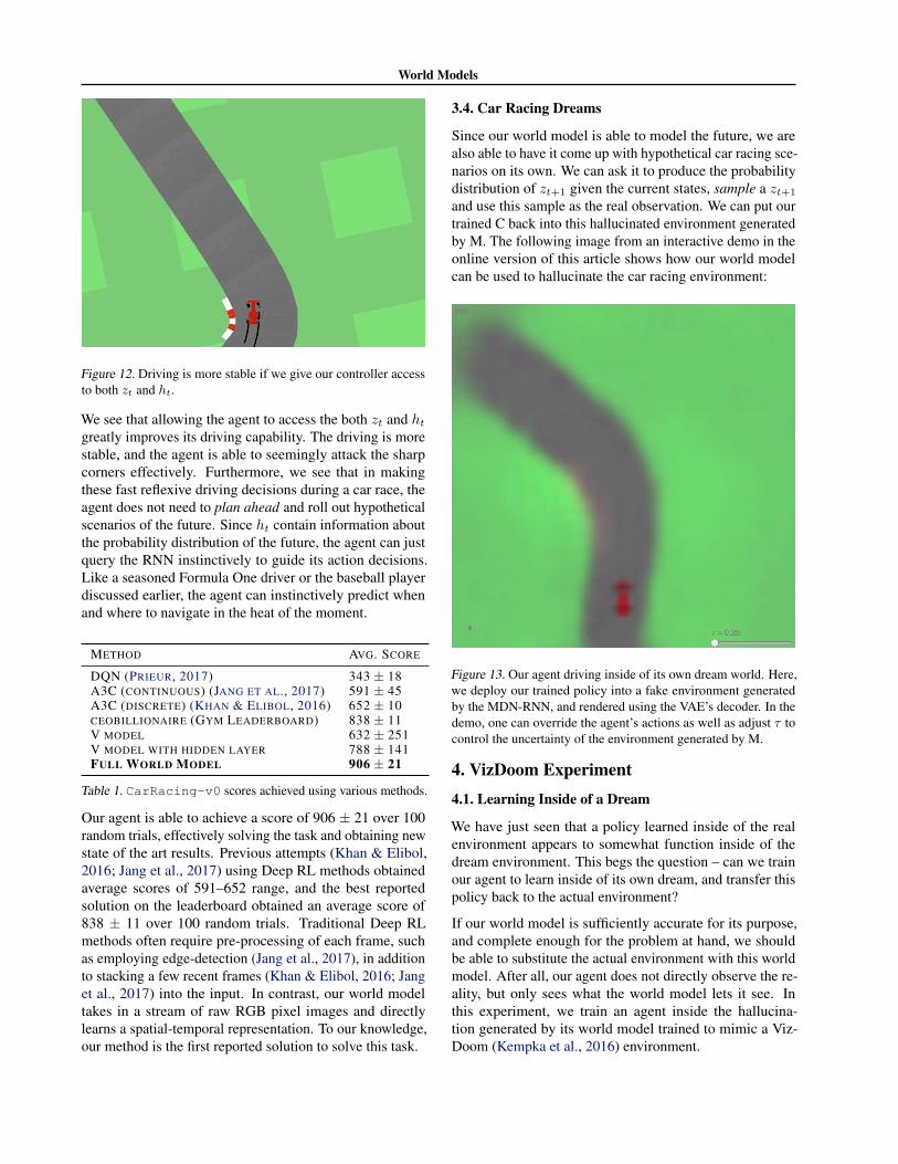
Figure 12. Driving is more stable if we give our controller accessto both zt and ht.

We see that allowing the agent to access the both zt and htgreatly improves its driving capability. The driving is morestable, and the agent is able to seemingly attack the sharpcorners effectively. Furthermore, we see that in makingthese fast reflexive driving decisions during a car race, theagent does not need to plan ahead and roll out hypotheticalscenarios of the future. Since ht contain information aboutthe probability distribution of the future, the agent can justquery the RNN instinctively to guide its action decisions.Like a seasoned Formula One driver or the baseball playerdiscussed earlier, the agent can instinctively predict whenand where to navigate in the heat of the moment.

METHOD AVG. SCORE

DQN (PRIEUR, 2017) 343 ± 18A3C (CONTINUOUS) (JANG ET AL., 2017) 591 ± 45A3C (DISCRETE) (KHAN & ELIBOL, 2016) 652 ± 10CEOBILLIONAIRE (GYM LEADERBOARD) 838 ± 11V MODEL 632 ± 251V MODEL WITH HIDDEN LAYER 788 ± 141FULL WORLD MODEL 906 ± 21

Table 1. CarRacing-v0 scores achieved using various methods.

Our agent is able to achieve a score of 906 ± 21 over 100random trials, effectively solving the task and obtaining newstate of the art results. Previous attempts (Khan & Elibol,2016; Jang et al., 2017) using Deep RL methods obtainedaverage scores of 591–652 range, and the best reportedsolution on the leaderboard obtained an average score of838 ± 11 over 100 random trials. Traditional Deep RLmethods often require pre-processing of each frame, suchas employing edge-detection (Jang et al., 2017), in additionto stacking a few recent frames (Khan & Elibol, 2016; Janget al., 2017) into the input. In contrast, our world modeltakes in a stream of raw RGB pixel images and directlylearns a spatial-temporal representation. To our knowledge,our method is the first reported solution to solve this task.

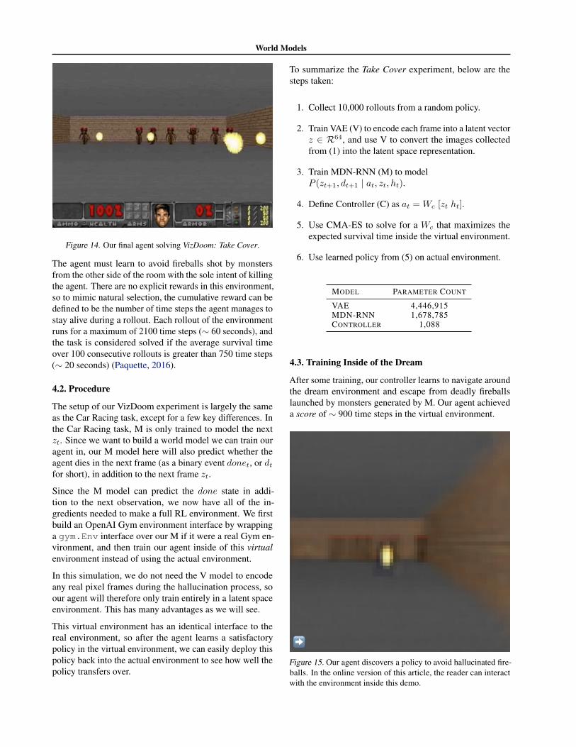
3.4. Car Racing Dreams

Since our world model is able to model the future, we arealso able to have it come up with hypothetical car racing sce-narios on its own. We can ask it to produce the probabilitydistribution of zt+1 given the current states, sample a zt+1

and use this sample as the real observation. We can put ourtrained C back into this hallucinated environment generatedby M. The following image from an interactive demo in theonline version of this article shows how our world modelcan be used to hallucinate the car racing environment:

Figure 13. Our agent driving inside of its own dream world. Here,we deploy our trained policy into a fake environment generatedby the MDN-RNN, and rendered using the VAE’s decoder. In thedemo, one can override the agent’s actions as well as adjust τ tocontrol the uncertainty of the environment generated by M.

4. VizDoom Experiment4.1. Learning Inside of a Dream

We have just seen that a policy learned inside of the realenvironment appears to somewhat function inside of thedream environment. This begs the question – can we trainour agent to learn inside of its own dream, and transfer thispolicy back to the actual environment?

If our world model is sufficiently accurate for its purpose,and complete enough for the problem at hand, we shouldbe able to substitute the actual environment with this worldmodel. After all, our agent does not directly observe the re-ality, but only sees what the world model lets it see. Inthis experiment, we train an agent inside the hallucina-tion generated by its world model trained to mimic a Viz-Doom (Kempka et al., 2016) environment.

World Models

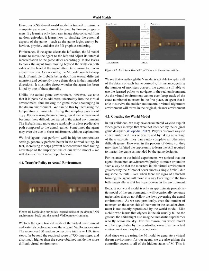
Figure 14. Our final agent solving VizDoom: Take Cover.

The agent must learn to avoid fireballs shot by monstersfrom the other side of the room with the sole intent of killingthe agent. There are no explicit rewards in this environment,so to mimic natural selection, the cumulative reward can bedefined to be the number of time steps the agent manages tostay alive during a rollout. Each rollout of the environmentruns for a maximum of 2100 time steps (∼ 60 seconds), andthe task is considered solved if the average survival timeover 100 consecutive rollouts is greater than 750 time steps(∼ 20 seconds) (Paquette, 2016).

4.2. Procedure

The setup of our VizDoom experiment is largely the sameas the Car Racing task, except for a few key differences. Inthe Car Racing task, M is only trained to model the nextzt. Since we want to build a world model we can train ouragent in, our M model here will also predict whether theagent dies in the next frame (as a binary event donet, or dtfor short), in addition to the next frame zt.

Since the M model can predict the done state in addi-tion to the next observation, we now have all of the in-gredients needed to make a full RL environment. We firstbuild an OpenAI Gym environment interface by wrappinga gym.Env interface over our M if it were a real Gym en-vironment, and then train our agent inside of this virtualenvironment instead of using the actual environment.

In this simulation, we do not need the V model to encodeany real pixel frames during the hallucination process, soour agent will therefore only train entirely in a latent spaceenvironment. This has many advantages as we will see.

This virtual environment has an identical interface to thereal environment, so after the agent learns a satisfactorypolicy in the virtual environment, we can easily deploy thispolicy back into the actual environment to see how well thepolicy transfers over.

To summarize the Take Cover experiment, below are thesteps taken:

1. Collect 10,000 rollouts from a random policy.

2. Train VAE (V) to encode each frame into a latent vectorz ∈ R64, and use V to convert the images collectedfrom (1) into the latent space representation.

3. Train MDN-RNN (M) to modelP (zt+1, dt+1 | at, zt, ht).

4. Define Controller (C) as at =Wc [zt ht].

5. Use CMA-ES to solve for a Wc that maximizes theexpected survival time inside the virtual environment.

6. Use learned policy from (5) on actual environment.

MODEL PARAMETER COUNT

VAE 4,446,915MDN-RNN 1,678,785CONTROLLER 1,088

4.3. Training Inside of the Dream

After some training, our controller learns to navigate aroundthe dream environment and escape from deadly fireballslaunched by monsters generated by M. Our agent achieveda score of ∼ 900 time steps in the virtual environment.

Figure 15. Our agent discovers a policy to avoid hallucinated fire-balls. In the online version of this article, the reader can interactwith the environment inside this demo.

World Models

Here, our RNN-based world model is trained to mimic acomplete game environment designed by human program-mers. By learning only from raw image data collected fromrandom episodes, it learns how to simulate the essentialaspects of the game – such as the game logic, enemy be-haviour, physics, and also the 3D graphics rendering.

For instance, if the agent selects the left action, the M modellearns to move the agent to the left and adjust its internalrepresentation of the game states accordingly. It also learnsto block the agent from moving beyond the walls on bothsides of the level if the agent attempts to move too far ineither direction. Occasionally, the M model needs to keeptrack of multiple fireballs being shot from several differentmonsters and coherently move them along in their intendeddirections. It must also detect whether the agent has beenkilled by one of these fireballs.

Unlike the actual game environment, however, we notethat it is possible to add extra uncertainty into the virtualenvironment, thus making the game more challenging inthe dream environment. We can do this by increasing thetemperature τ parameter during the sampling process ofzt+1. By increasing the uncertainty, our dream environmentbecomes more difficult compared to the actual environment.The fireballs may move more randomly in a less predictablepath compared to the actual game. Sometimes the agentmay even die due to sheer misfortune, without explanation.

We find agents that perform well in higher temperaturesettings generally perform better in the normal setting. Infact, increasing τ helps prevent our controller from takingadvantage of the imperfections of our world model – wewill discuss this in more depth later on.

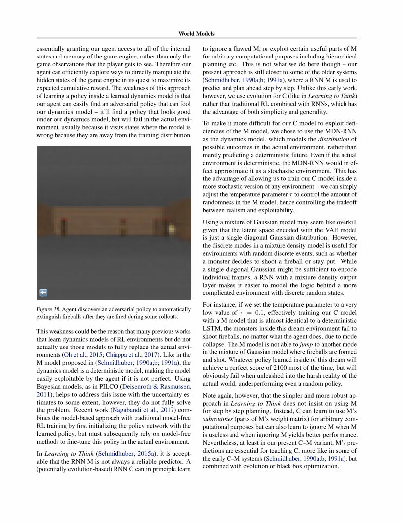
4.4. Transfer Policy to Actual Environment

Figure 16. Deploying our policy learned inside of the dream RNNenvironment back into the actual VizDoom environment.

We took the agent trained inside of the virtual environmentand tested its performance on the original VizDoom scenario.The score over 100 random consecutive trials is∼ 1100 timesteps, far beyond the required score of 750 time steps, andalso much higher than the score obtained inside the moredifficult virtual environment.

Figure 17. An interactive VAE of Doom in the online article.

We see that even though the V model is not able to capture allof the details of each frame correctly, for instance, gettingthe number of monsters correct, the agent is still able touse the learned policy to navigate in the real environment.As the virtual environment cannot even keep track of theexact number of monsters in the first place, an agent that isable to survive the noisier and uncertain virtual nightmareenvironment will thrive in the original, cleaner environment.

4.5. Cheating the World Model

In our childhood, we may have encountered ways to exploitvideo games in ways that were not intended by the originalgame designer (Wikipedia, 2017). Players discover ways tocollect unlimited lives or health, and by taking advantageof these exploits, they can easily complete an otherwisedifficult game. However, in the process of doing so, theymay have forfeited the opportunity to learn the skill requiredto master the game as intended by the game designer.

For instance, in our initial experiments, we noticed that ouragent discovered an adversarial policy to move around insuch a way so that the monsters in this virtual environmentgoverned by the M model never shoots a single fireball dur-ing some rollouts. Even when there are signs of a fireballforming, the agent will move in a way to extinguish the fire-balls magically as if it has superpowers in the environment.

Because our world model is only an approximate probabilis-tic model of the environment, it will occasionally generatetrajectories that do not follow the laws governing the actualenvironment. As we saw previously, even the number ofmonsters on the other side of the room in the actual environ-ment is not exactly reproduced by the world model. Likea child who learns that objects in the air usually fall to theground, the child might also imagine unrealistic superheroeswho fly across the sky. For this reason, our world modelwill be exploitable by the controller, even if in the actualenvironment such exploits do not exist.

And since we are using the M model to generate a virtualdream environment for our agent, we are also giving thecontroller access to all of the hidden states of M. This is

World Models

essentially granting our agent access to all of the internalstates and memory of the game engine, rather than only thegame observations that the player gets to see. Therefore ouragent can efficiently explore ways to directly manipulate thehidden states of the game engine in its quest to maximize itsexpected cumulative reward. The weakness of this approachof learning a policy inside a learned dynamics model is thatour agent can easily find an adversarial policy that can foolour dynamics model – it’ll find a policy that looks goodunder our dynamics model, but will fail in the actual envi-ronment, usually because it visits states where the model iswrong because they are away from the training distribution.

Figure 18. Agent discovers an adversarial policy to automaticallyextinguish fireballs after they are fired during some rollouts.

This weakness could be the reason that many previous worksthat learn dynamics models of RL environments but do notactually use those models to fully replace the actual envi-ronments (Oh et al., 2015; Chiappa et al., 2017). Like in theM model proposed in (Schmidhuber, 1990a;b; 1991a), thedynamics model is a deterministic model, making the modeleasily exploitable by the agent if it is not perfect. UsingBayesian models, as in PILCO (Deisenroth & Rasmussen,2011), helps to address this issue with the uncertainty es-timates to some extent, however, they do not fully solvethe problem. Recent work (Nagabandi et al., 2017) com-bines the model-based approach with traditional model-freeRL training by first initializing the policy network with thelearned policy, but must subsequently rely on model-freemethods to fine-tune this policy in the actual environment.

In Learning to Think (Schmidhuber, 2015a), it is accept-able that the RNN M is not always a reliable predictor. A(potentially evolution-based) RNN C can in principle learn

to ignore a flawed M, or exploit certain useful parts of Mfor arbitrary computational purposes including hierarchicalplanning etc. This is not what we do here though – ourpresent approach is still closer to some of the older systems(Schmidhuber, 1990a;b; 1991a), where a RNN M is used topredict and plan ahead step by step. Unlike this early work,however, we use evolution for C (like in Learning to Think)rather than traditional RL combined with RNNs, which hasthe advantage of both simplicity and generality.

To make it more difficult for our C model to exploit defi-ciencies of the M model, we chose to use the MDN-RNNas the dynamics model, which models the distribution ofpossible outcomes in the actual environment, rather thanmerely predicting a deterministic future. Even if the actualenvironment is deterministic, the MDN-RNN would in ef-fect approximate it as a stochastic environment. This hasthe advantage of allowing us to train our C model inside amore stochastic version of any environment – we can simplyadjust the temperature parameter τ to control the amount ofrandomness in the M model, hence controlling the tradeoffbetween realism and exploitability.

Using a mixture of Gaussian model may seem like overkillgiven that the latent space encoded with the VAE modelis just a single diagonal Gaussian distribution. However,the discrete modes in a mixture density model is useful forenvironments with random discrete events, such as whethera monster decides to shoot a fireball or stay put. Whilea single diagonal Gaussian might be sufficient to encodeindividual frames, a RNN with a mixture density outputlayer makes it easier to model the logic behind a morecomplicated environment with discrete random states.

For instance, if we set the temperature parameter to a verylow value of τ = 0.1, effectively training our C modelwith a M model that is almost identical to a deterministicLSTM, the monsters inside this dream environment fail toshoot fireballs, no matter what the agent does, due to modecollapse. The M model is not able to jump to another modein the mixture of Gaussian model where fireballs are formedand shot. Whatever policy learned inside of this dream willachieve a perfect score of 2100 most of the time, but willobviously fail when unleashed into the harsh reality of theactual world, underperforming even a random policy.

Note again, however, that the simpler and more robust ap-proach in Learning to Think does not insist on using Mfor step by step planning. Instead, C can learn to use M’ssubroutines (parts of M’s weight matrix) for arbitrary com-putational purposes but can also learn to ignore M when Mis useless and when ignoring M yields better performance.Nevertheless, at least in our present C–M variant, M’s pre-dictions are essential for teaching C, more like in some ofthe early C–M systems (Schmidhuber, 1990a;b; 1991a), butcombined with evolution or black box optimization.

World Models

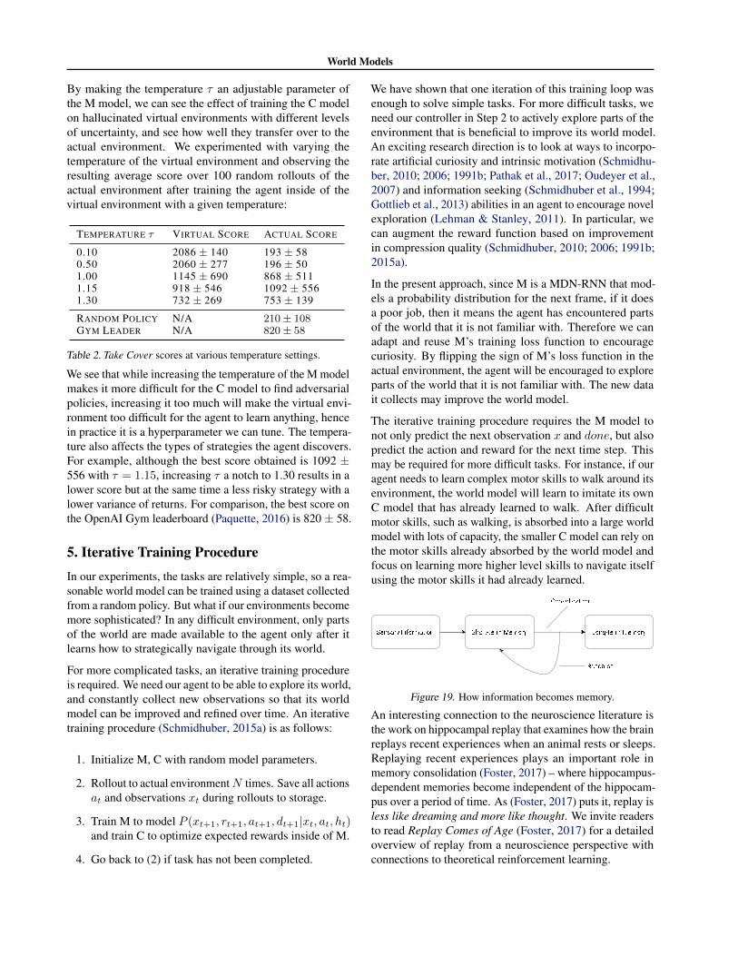
By making the temperature τ an adjustable parameter ofthe M model, we can see the effect of training the C modelon hallucinated virtual environments with different levelsof uncertainty, and see how well they transfer over to theactual environment. We experimented with varying thetemperature of the virtual environment and observing theresulting average score over 100 random rollouts of theactual environment after training the agent inside of thevirtual environment with a given temperature:

TEMPERATURE τ VIRTUAL SCORE ACTUAL SCORE

0.10 2086 ± 140 193 ± 580.50 2060 ± 277 196 ± 501.00 1145 ± 690 868 ± 5111.15 918 ± 546 1092 ± 5561.30 732 ± 269 753 ± 139

RANDOM POLICY N/A 210± 108GYM LEADER N/A 820± 58

Table 2. Take Cover scores at various temperature settings.

We see that while increasing the temperature of the M modelmakes it more difficult for the C model to find adversarialpolicies, increasing it too much will make the virtual envi-ronment too difficult for the agent to learn anything, hencein practice it is a hyperparameter we can tune. The tempera-ture also affects the types of strategies the agent discovers.For example, although the best score obtained is 1092 ±556 with τ = 1.15, increasing τ a notch to 1.30 results in alower score but at the same time a less risky strategy with alower variance of returns. For comparison, the best score onthe OpenAI Gym leaderboard (Paquette, 2016) is 820 ± 58.

5. Iterative Training ProcedureIn our experiments, the tasks are relatively simple, so a rea-sonable world model can be trained using a dataset collectedfrom a random policy. But what if our environments becomemore sophisticated? In any difficult environment, only partsof the world are made available to the agent only after itlearns how to strategically navigate through its world.

For more complicated tasks, an iterative training procedureis required. We need our agent to be able to explore its world,and constantly collect new observations so that its worldmodel can be improved and refined over time. An iterativetraining procedure (Schmidhuber, 2015a) is as follows:

1. Initialize M, C with random model parameters.

2. Rollout to actual environmentN times. Save all actionsat and observations xt during rollouts to storage.

3. Train M to model P (xt+1, rt+1, at+1, dt+1|xt, at, ht)and train C to optimize expected rewards inside of M.

4. Go back to (2) if task has not been completed.

We have shown that one iteration of this training loop wasenough to solve simple tasks. For more difficult tasks, weneed our controller in Step 2 to actively explore parts of theenvironment that is beneficial to improve its world model.An exciting research direction is to look at ways to incorpo-rate artificial curiosity and intrinsic motivation (Schmidhu-ber, 2010; 2006; 1991b; Pathak et al., 2017; Oudeyer et al.,2007) and information seeking (Schmidhuber et al., 1994;Gottlieb et al., 2013) abilities in an agent to encourage novelexploration (Lehman & Stanley, 2011). In particular, wecan augment the reward function based on improvementin compression quality (Schmidhuber, 2010; 2006; 1991b;2015a).

In the present approach, since M is a MDN-RNN that mod-els a probability distribution for the next frame, if it doesa poor job, then it means the agent has encountered partsof the world that it is not familiar with. Therefore we canadapt and reuse M’s training loss function to encouragecuriosity. By flipping the sign of M’s loss function in theactual environment, the agent will be encouraged to exploreparts of the world that it is not familiar with. The new datait collects may improve the world model.

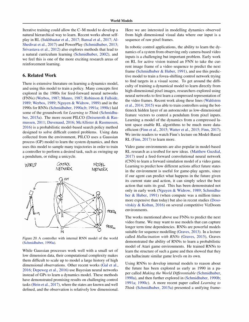
The iterative training procedure requires the M model tonot only predict the next observation x and done, but alsopredict the action and reward for the next time step. Thismay be required for more difficult tasks. For instance, if ouragent needs to learn complex motor skills to walk around itsenvironment, the world model will learn to imitate its ownC model that has already learned to walk. After difficultmotor skills, such as walking, is absorbed into a large worldmodel with lots of capacity, the smaller C model can rely onthe motor skills already absorbed by the world model andfocus on learning more higher level skills to navigate itselfusing the motor skills it had already learned.

Figure 19. How information becomes memory.

An interesting connection to the neuroscience literature isthe work on hippocampal replay that examines how the brainreplays recent experiences when an animal rests or sleeps.Replaying recent experiences plays an important role inmemory consolidation (Foster, 2017) – where hippocampus-dependent memories become independent of the hippocam-pus over a period of time. As (Foster, 2017) puts it, replay isless like dreaming and more like thought. We invite readersto read Replay Comes of Age (Foster, 2017) for a detailedoverview of replay from a neuroscience perspective withconnections to theoretical reinforcement learning.

World Models

Iterative training could allow the C–M model to develop anatural hierarchical way to learn. Recent works about self-play in RL (Sukhbaatar et al., 2017; Bansal et al., 2017; Al-Shedivat et al., 2017) and PowerPlay (Schmidhuber, 2013;Srivastava et al., 2012) also explores methods that lead toa natural curriculum learning (Schmidhuber, 2002), andwe feel this is one of the more exciting research areas ofreinforcement learning.

6. Related WorkThere is extensive literature on learning a dynamics model,and using this model to train a policy. Many concepts firstexplored in the 1980s for feed-forward neural networks(FNNs) (Werbos, 1987; Munro, 1987; Robinson & Fallside,1989; Werbos, 1989; Nguyen & Widrow, 1989) and in the1990s for RNNs (Schmidhuber, 1990a;b; 1991a; 1990c) laidsome of the groundwork for Learning to Think (Schmidhu-ber, 2015a). The more recent PILCO (Deisenroth & Ras-mussen, 2011; Duvenaud, 2016; McAllister & Rasmussen,2016) is a probabilistic model-based search policy methoddesigned to solve difficult control problems. Using datacollected from the environment, PILCO uses a Gaussianprocess (GP) model to learn the system dynamics, and thenuses this model to sample many trajectories in order to traina controller to perform a desired task, such as swinging upa pendulum, or riding a unicycle.

Figure 20. A controller with internal RNN model of the world(Schmidhuber, 1990a).

While Gaussian processes work well with a small set oflow dimension data, their computational complexity makesthem difficult to scale up to model a large history of highdimensional observations. Other recent works (Gal et al.,2016; Depeweg et al., 2016) use Bayesian neural networksinstead of GPs to learn a dynamics model. These methodshave demonstrated promising results on challenging controltasks (Hein et al., 2017), where the states are known and welldefined, and the observation is relatively low dimensional.

Here we are interested in modelling dynamics observedfrom high dimensional visual data where our input is asequence of raw pixel frames.

In robotic control applications, the ability to learn the dy-namics of a system from observing only camera-based videoinputs is a challenging but important problem. Early workon RL for active vision trained an FNN to take the cur-rent image frame of a video sequence to predict the nextframe (Schmidhuber & Huber, 1991), and use this predic-tive model to train a fovea-shifting control network tryingto find targets in a visual scene. To get around the diffi-culty of training a dynamical model to learn directly fromhigh-dimensional pixel images, researchers explored usingneural networks to first learn a compressed representation ofthe video frames. Recent work along these lines (Wahlstrmet al., 2014; 2015) was able to train controllers using the bot-tleneck hidden layer of an autoencoder as low-dimensionalfeature vectors to control a pendulum from pixel inputs.Learning a model of the dynamics from a compressed la-tent space enable RL algorithms to be much more data-efficient (Finn et al., 2015; Watter et al., 2015; Finn, 2017).We invite readers to watch Finn’s lecture on Model-BasedRL (Finn, 2017) to learn more.

Video game environments are also popular in model-basedRL research as a testbed for new ideas. (Matthew Guzdial,2017) used a feed-forward convolutional neural network(CNN) to learn a forward simulation model of a video game.Learning to predict how different actions affect future statesin the environment is useful for game-play agents, sinceif our agent can predict what happens in the future givenits current state and action, it can simply select the bestaction that suits its goal. This has been demonstrated notonly in early work (Nguyen & Widrow, 1989; Schmidhu-ber & Huber, 1991) (when compute was a million timesmore expensive than today) but also in recent studies (Doso-vitskiy & Koltun, 2016) on several competitive VizDoomenvironments.

The works mentioned above use FNNs to predict the nextvideo frame. We may want to use models that can capturelonger term time dependencies. RNNs are powerful modelssuitable for sequence modelling (Graves, 2013). In a lecturecalled Hallucination with RNNs (Graves, 2015), Gravesdemonstrated the ability of RNNs to learn a probabilisticmodel of Atari game environments. He trained RNNs tolearn the structure of such a game and then showed that theycan hallucinate similar game levels on its own.

Using RNNs to develop internal models to reason aboutthe future has been explored as early as 1990 in a pa-per called Making the World Differentiable (Schmidhuber,1990a), and then further explored in (Schmidhuber, 1990b;1991a; 1990c). A more recent paper called Learning toThink (Schmidhuber, 2015a) presented a unifying frame-

World Models

work for building a RNN-based general problem solver thatcan learn a world model of its environment and also learn toreason about the future using this model. Subsequent workshave used RNN-based models to generate many frames intothe future (Chiappa et al., 2017; Oh et al., 2015; Denton& Birodkar, 2017), and also as an internal model to reasonabout the future (Silver et al., 2016; Weber et al., 2017;Watters et al., 2017).

In this work, we used evolution strategies to train our con-troller, as it offers many benefits. For instance, we only needto provide the optimizer with the final cumulative reward,rather than the entire history. ES is also easy to parallelize –we can launch many instances of rollout with differentsolutions to many workers and quickly compute a set ofcumulative rewards in parallel. Recent works (Fernandoet al., 2017; Salimans et al., 2017; Ha, 2017b; Stanley &Clune, 2017) have confirmed that ES is a viable alternativeto traditional Deep RL methods on many strong baselines.

Before the popularity of Deep RL methods (Mnih et al.,2013), evolution-based algorithms have been shown to beeffective at solving RL tasks (Stanley & Miikkulainen, 2002;Gomez et al., 2008; Gomez & Schmidhuber, 2005; Gauci& Stanley, 2010; Sehnke et al., 2010; Miikkulainen, 2013).Evolution-based algorithms have even been able to solvedifficult RL tasks from high dimensional pixel inputs (Kout-nik et al., 2013; Hausknecht et al., 2013; Parker & Bryant,2012). More recent works (Alvernaz & Togelius, 2017)combine VAE and ES, which is similar to our approach.

7. Discussion

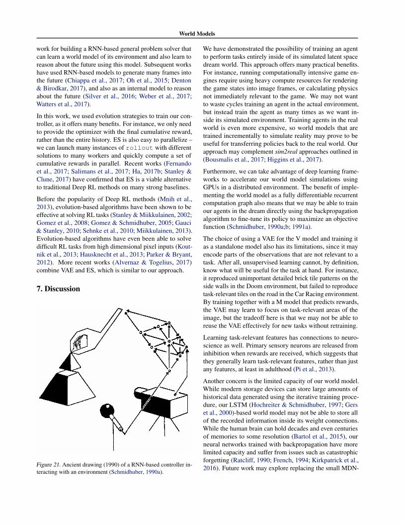
Figure 21. Ancient drawing (1990) of a RNN-based controller in-teracting with an environment (Schmidhuber, 1990a).

We have demonstrated the possibility of training an agentto perform tasks entirely inside of its simulated latent spacedream world. This approach offers many practical benefits.For instance, running computationally intensive game en-gines require using heavy compute resources for renderingthe game states into image frames, or calculating physicsnot immediately relevant to the game. We may not wantto waste cycles training an agent in the actual environment,but instead train the agent as many times as we want in-side its simulated environment. Training agents in the realworld is even more expensive, so world models that aretrained incrementally to simulate reality may prove to beuseful for transferring policies back to the real world. Ourapproach may complement sim2real approaches outlined in(Bousmalis et al., 2017; Higgins et al., 2017).

Furthermore, we can take advantage of deep learning frame-works to accelerate our world model simulations usingGPUs in a distributed environment. The benefit of imple-menting the world model as a fully differentiable recurrentcomputation graph also means that we may be able to trainour agents in the dream directly using the backpropagationalgorithm to fine-tune its policy to maximize an objectivefunction (Schmidhuber, 1990a;b; 1991a).

The choice of using a VAE for the V model and training itas a standalone model also has its limitations, since it mayencode parts of the observations that are not relevant to atask. After all, unsupervised learning cannot, by definition,know what will be useful for the task at hand. For instance,it reproduced unimportant detailed brick tile patterns on theside walls in the Doom environment, but failed to reproducetask-relevant tiles on the road in the Car Racing environment.By training together with a M model that predicts rewards,the VAE may learn to focus on task-relevant areas of theimage, but the tradeoff here is that we may not be able toreuse the VAE effectively for new tasks without retraining.

Learning task-relevant features has connections to neuro-science as well. Primary sensory neurons are released frominhibition when rewards are received, which suggests thatthey generally learn task-relevant features, rather than justany features, at least in adulthood (Pi et al., 2013).

Another concern is the limited capacity of our world model.While modern storage devices can store large amounts ofhistorical data generated using the iterative training proce-dure, our LSTM (Hochreiter & Schmidhuber, 1997; Gerset al., 2000)-based world model may not be able to store allof the recorded information inside its weight connections.While the human brain can hold decades and even centuriesof memories to some resolution (Bartol et al., 2015), ourneural networks trained with backpropagation have morelimited capacity and suffer from issues such as catastrophicforgetting (Ratcliff, 1990; French, 1994; Kirkpatrick et al.,2016). Future work may explore replacing the small MDN-

World Models

RNN network with higher capacity models (Shazeer et al.,2017; Ha et al., 2016; Suarez, 2017; van den Oord et al.,2016; Vaswani et al., 2017), or incorporating an externalmemory module (Gemici et al., 2017), if we want our agentto learn to explore more complicated worlds.

Like early RNN-based C–M systems (Schmidhuber,1990a;b; 1991a; 1990c), ours simulates possible futurestime step by time step, without profiting from human-likehierarchical planning or abstract reasoning, which often ig-nores irrelevant spatial-temporal details. However, the moregeneral Learning To Think (Schmidhuber, 2015a) approachis not limited to this rather naive approach. Instead it allowsa recurrent C to learn to address subroutines of the recurrentM, and reuse them for problem solving in arbitrary com-putable ways, e.g., through hierarchical planning or otherkinds of exploiting parts of M’s program-like weight matrix.A recent One Big Net (Schmidhuber, 2018) extension of theC–M approach collapses C and M into a single network, anduses PowerPlay-like (Schmidhuber, 2013; Srivastava et al.,2012) behavioural replay (where the behaviour of a teachernet is compressed into a student net (Schmidhuber, 1992))to avoid forgetting old prediction and control skills whenlearning new ones. Experiments with those more generalapproaches are left for future work.

AcknowledgementsWe would like to thank Blake Richards, Kai Arulkumaran,Ankur Handa, Kory Mathewson, Kyle McDonald, DennyBritz, Elwin Ha and Natasha Jaques for their thoughtfulfeedback on this article, and for offering their valuable per-spectives and insights from their areas of expertise.

The interactive online version of this article was built usingdistill.pub’s web technology. We would like to thankChris Olah and the rest of the Distill editorial team fortheir valuable feedback and generous editorial support, inaddition to supporting the use of their Distill technology.

The interative demos on worldmodels.github.iowere all built using p5.js. Deploying all of these machinelearning models in a web browser was made possible withdeeplearn.js, a hardware-accelerated machine learn-ing framework for the browser, developed by the People+AIResearch Initiative (PAIR) team at Google. A special thanksgoes to Nikhil Thorat and Daniel Smilkov for their helpduring the development process.

We would to extend our thanks to Alex Graves, Douglas Eck,Mike Schuster, Rajat Monga, Vincent Vanhoucke, Jeff Deanand the Google Brain team for helpful feedback and forencouraging us to explore this area of research. Experimentswere performed on Ubuntu virtual machines provided byGoogle Cloud Platform. Any errors here are our own anddo not reflect opinions of our proofreaders and colleagues.

A. AppendixIn this section we will describe in more details the modelsand training methods used in this work.

A.1. Variational Autoencoder

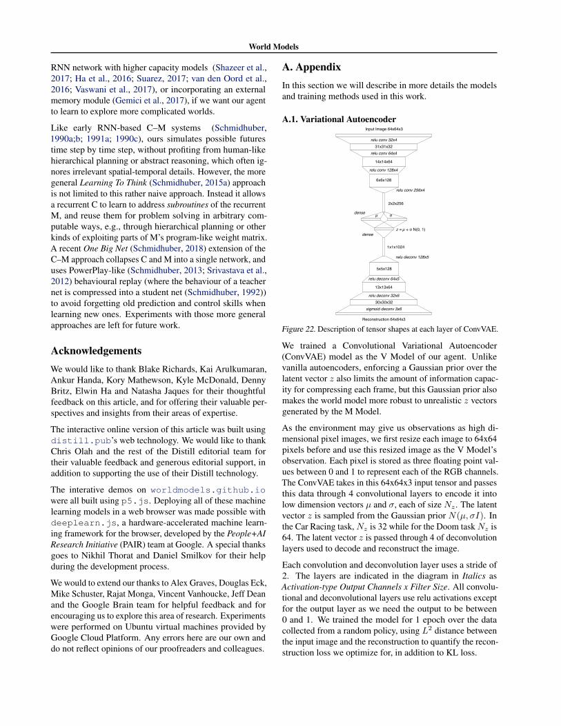
Figure 22. Description of tensor shapes at each layer of ConvVAE.

We trained a Convolutional Variational Autoencoder(ConvVAE) model as the V Model of our agent. Unlikevanilla autoencoders, enforcing a Gaussian prior over thelatent vector z also limits the amount of information capac-ity for compressing each frame, but this Gaussian prior alsomakes the world model more robust to unrealistic z vectorsgenerated by the M Model.

As the environment may give us observations as high di-mensional pixel images, we first resize each image to 64x64pixels before and use this resized image as the V Model’sobservation. Each pixel is stored as three floating point val-ues between 0 and 1 to represent each of the RGB channels.The ConvVAE takes in this 64x64x3 input tensor and passesthis data through 4 convolutional layers to encode it intolow dimension vectors µ and σ, each of size Nz . The latentvector z is sampled from the Gaussian prior N(µ, σI). Inthe Car Racing task, Nz is 32 while for the Doom taskNz is64. The latent vector z is passed through 4 of deconvolutionlayers used to decode and reconstruct the image.

Each convolution and deconvolution layer uses a stride of2. The layers are indicated in the diagram in Italics asActivation-type Output Channels x Filter Size. All convolu-tional and deconvolutional layers use relu activations exceptfor the output layer as we need the output to be between0 and 1. We trained the model for 1 epoch over the datacollected from a random policy, using L2 distance betweenthe input image and the reconstruction to quantify the recon-struction loss we optimize for, in addition to KL loss.

World Models

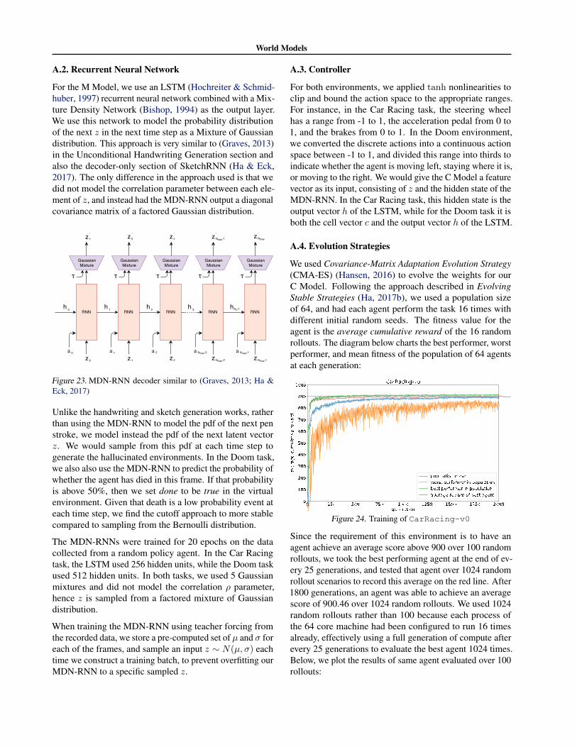
A.2. Recurrent Neural Network

For the M Model, we use an LSTM (Hochreiter & Schmid-huber, 1997) recurrent neural network combined with a Mix-ture Density Network (Bishop, 1994) as the output layer.We use this network to model the probability distributionof the next z in the next time step as a Mixture of Gaussiandistribution. This approach is very similar to (Graves, 2013)in the Unconditional Handwriting Generation section andalso the decoder-only section of SketchRNN (Ha & Eck,2017). The only difference in the approach used is that wedid not model the correlation parameter between each ele-ment of z, and instead had the MDN-RNN output a diagonalcovariance matrix of a factored Gaussian distribution.

Figure 23. MDN-RNN decoder similar to (Graves, 2013; Ha &Eck, 2017)

Unlike the handwriting and sketch generation works, ratherthan using the MDN-RNN to model the pdf of the next penstroke, we model instead the pdf of the next latent vectorz. We would sample from this pdf at each time step togenerate the hallucinated environments. In the Doom task,we also also use the MDN-RNN to predict the probability ofwhether the agent has died in this frame. If that probabilityis above 50%, then we set done to be true in the virtualenvironment. Given that death is a low probability event ateach time step, we find the cutoff approach to more stablecompared to sampling from the Bernoulli distribution.

The MDN-RNNs were trained for 20 epochs on the datacollected from a random policy agent. In the Car Racingtask, the LSTM used 256 hidden units, while the Doom taskused 512 hidden units. In both tasks, we used 5 Gaussianmixtures and did not model the correlation ρ parameter,hence z is sampled from a factored mixture of Gaussiandistribution.

When training the MDN-RNN using teacher forcing fromthe recorded data, we store a pre-computed set of µ and σ foreach of the frames, and sample an input z ∼ N(µ, σ) eachtime we construct a training batch, to prevent overfitting ourMDN-RNN to a specific sampled z.

A.3. Controller

For both environments, we applied tanh nonlinearities toclip and bound the action space to the appropriate ranges.For instance, in the Car Racing task, the steering wheelhas a range from -1 to 1, the acceleration pedal from 0 to1, and the brakes from 0 to 1. In the Doom environment,we converted the discrete actions into a continuous actionspace between -1 to 1, and divided this range into thirds toindicate whether the agent is moving left, staying where it is,or moving to the right. We would give the C Model a featurevector as its input, consisting of z and the hidden state of theMDN-RNN. In the Car Racing task, this hidden state is theoutput vector h of the LSTM, while for the Doom task it isboth the cell vector c and the output vector h of the LSTM.

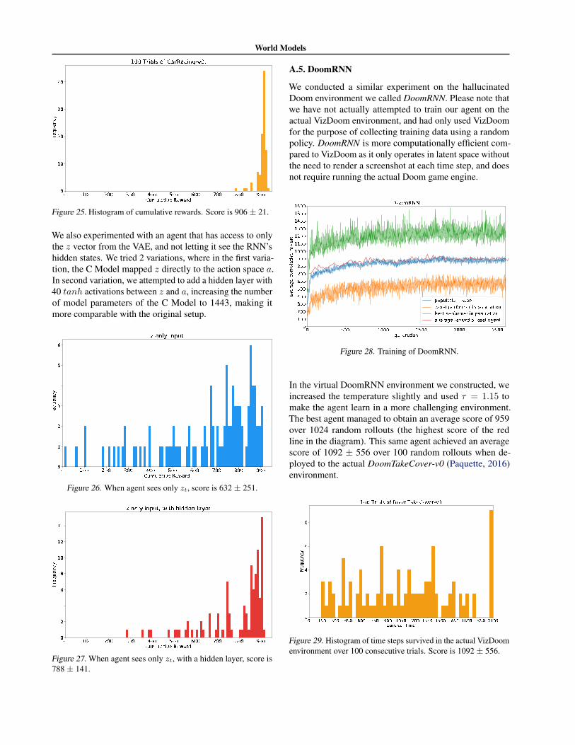
A.4. Evolution Strategies

We used Covariance-Matrix Adaptation Evolution Strategy(CMA-ES) (Hansen, 2016) to evolve the weights for ourC Model. Following the approach described in EvolvingStable Strategies (Ha, 2017b), we used a population sizeof 64, and had each agent perform the task 16 times withdifferent initial random seeds. The fitness value for theagent is the average cumulative reward of the 16 randomrollouts. The diagram below charts the best performer, worstperformer, and mean fitness of the population of 64 agentsat each generation:

Figure 24. Training of CarRacing-v0

Since the requirement of this environment is to have anagent achieve an average score above 900 over 100 randomrollouts, we took the best performing agent at the end of ev-ery 25 generations, and tested that agent over 1024 randomrollout scenarios to record this average on the red line. After1800 generations, an agent was able to achieve an averagescore of 900.46 over 1024 random rollouts. We used 1024random rollouts rather than 100 because each process ofthe 64 core machine had been configured to run 16 timesalready, effectively using a full generation of compute afterevery 25 generations to evaluate the best agent 1024 times.Below, we plot the results of same agent evaluated over 100rollouts:

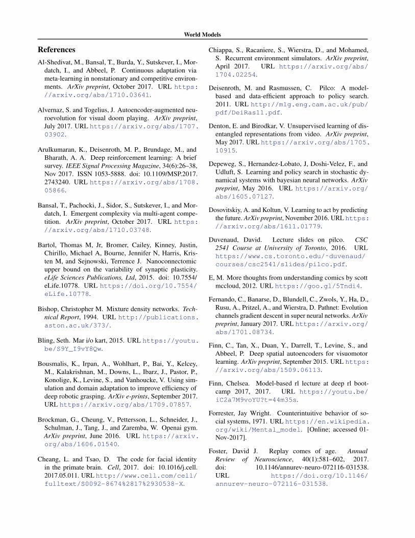
World Models

Figure 25. Histogram of cumulative rewards. Score is 906 ± 21.

We also experimented with an agent that has access to onlythe z vector from the VAE, and not letting it see the RNN’shidden states. We tried 2 variations, where in the first varia-tion, the C Model mapped z directly to the action space a.In second variation, we attempted to add a hidden layer with40 tanh activations between z and a, increasing the numberof model parameters of the C Model to 1443, making itmore comparable with the original setup.

Figure 26. When agent sees only zt, score is 632 ± 251.

Figure 27. When agent sees only zt, with a hidden layer, score is788 ± 141.

A.5. DoomRNN

We conducted a similar experiment on the hallucinatedDoom environment we called DoomRNN. Please note thatwe have not actually attempted to train our agent on theactual VizDoom environment, and had only used VizDoomfor the purpose of collecting training data using a randompolicy. DoomRNN is more computationally efficient com-pared to VizDoom as it only operates in latent space withoutthe need to render a screenshot at each time step, and doesnot require running the actual Doom game engine.

Figure 28. Training of DoomRNN.

In the virtual DoomRNN environment we constructed, weincreased the temperature slightly and used τ = 1.15 tomake the agent learn in a more challenging environment.The best agent managed to obtain an average score of 959over 1024 random rollouts (the highest score of the redline in the diagram). This same agent achieved an averagescore of 1092 ± 556 over 100 random rollouts when de-ployed to the actual DoomTakeCover-v0 (Paquette, 2016)environment.

Figure 29. Histogram of time steps survived in the actual VizDoomenvironment over 100 consecutive trials. Score is 1092 ± 556.

World Models

ReferencesAl-Shedivat, M., Bansal, T., Burda, Y., Sutskever, I., Mor-

datch, I., and Abbeel, P. Continuous adaptation viameta-learning in nonstationary and competitive environ-ments. ArXiv preprint, October 2017. URL https://arxiv.org/abs/1710.03641.

Alvernaz, S. and Togelius, J. Autoencoder-augmented neu-roevolution for visual doom playing. ArXiv preprint,July 2017. URL https://arxiv.org/abs/1707.03902.

Arulkumaran, K., Deisenroth, M. P., Brundage, M., andBharath, A. A. Deep reinforcement learning: A briefsurvey. IEEE Signal Processing Magazine, 34(6):26–38,Nov 2017. ISSN 1053-5888. doi: 10.1109/MSP.2017.2743240. URL https://arxiv.org/abs/1708.05866.

Bansal, T., Pachocki, J., Sidor, S., Sutskever, I., and Mor-datch, I. Emergent complexity via multi-agent compe-tition. ArXiv preprint, October 2017. URL https://arxiv.org/abs/1710.03748.

Bartol, Thomas M, Jr, Bromer, Cailey, Kinney, Justin,Chirillo, Michael A, Bourne, Jennifer N, Harris, Kris-ten M, and Sejnowski, Terrence J. Nanoconnectomicupper bound on the variability of synaptic plasticity.eLife Sciences Publications, Ltd, 2015. doi: 10.7554/eLife.10778. URL https://doi.org/10.7554/eLife.10778.

Bishop, Christopher M. Mixture density networks. Tech-nical Report, 1994. URL http://publications.aston.ac.uk/373/.

Bling, Seth. Mar i/o kart, 2015. URL https://youtu.be/S9Y_I9vY8Qw.

Bousmalis, K., Irpan, A., Wohlhart, P., Bai, Y., Kelcey,M., Kalakrishnan, M., Downs, L., Ibarz, J., Pastor, P.,Konolige, K., Levine, S., and Vanhoucke, V. Using sim-ulation and domain adaptation to improve efficiency ofdeep robotic grasping. ArXiv e-prints, September 2017.URL https://arxiv.org/abs/1709.07857.

Brockman, G., Cheung, V., Pettersson, L., Schneider, J.,Schulman, J., Tang, J., and Zaremba, W. Openai gym.ArXiv preprint, June 2016. URL https://arxiv.org/abs/1606.01540.

Cheang, L. and Tsao, D. The code for facial identityin the primate brain. Cell, 2017. doi: 10.1016/j.cell.2017.05.011. URL http://www.cell.com/cell/fulltext/S0092-8674%2817%2930538-X.

Chiappa, S., Racaniere, S., Wierstra, D., and Mohamed,S. Recurrent environment simulators. ArXiv preprint,April 2017. URL https://arxiv.org/abs/1704.02254.

Deisenroth, M. and Rasmussen, C. Pilco: A model-based and data-efficient approach to policy search.2011. URL http://mlg.eng.cam.ac.uk/pub/pdf/DeiRas11.pdf.

Denton, E. and Birodkar, V. Unsupervised learning of dis-entangled representations from video. ArXiv preprint,May 2017. URL https://arxiv.org/abs/1705.10915.

Depeweg, S., Hernandez-Lobato, J, Doshi-Velez, F., andUdluft, S. Learning and policy search in stochastic dy-namical systems with bayesian neural networks. ArXivpreprint, May 2016. URL https://arxiv.org/abs/1605.07127.

Dosovitskiy, A. and Koltun, V. Learning to act by predictingthe future. ArXiv preprint, November 2016. URL https://arxiv.org/abs/1611.01779.

Duvenaud, David. Lecture slides on pilco. CSC2541 Course at University of Toronto, 2016. URLhttps://www.cs.toronto.edu/˜duvenaud/courses/csc2541/slides/pilco.pdf.

E, M. More thoughts from understanding comics by scottmccloud, 2012. URL https://goo.gl/5Tndi4.

Fernando, C., Banarse, D., Blundell, C., Zwols, Y., Ha, D.,Rusu, A., Pritzel, A., and Wierstra, D. Pathnet: Evolutionchannels gradient descent in super neural networks. ArXivpreprint, January 2017. URL https://arxiv.org/abs/1701.08734.

Finn, C., Tan, X., Duan, Y., Darrell, T., Levine, S., andAbbeel, P. Deep spatial autoencoders for visuomotorlearning. ArXiv preprint, September 2015. URL https://arxiv.org/abs/1509.06113.

Finn, Chelsea. Model-based rl lecture at deep rl boot-camp 2017, 2017. URL https://youtu.be/iC2a7M9voYU?t=44m35s.

Forrester, Jay Wright. Counterintuitive behavior of so-cial systems, 1971. URL https://en.wikipedia.org/wiki/Mental_model. [Online; accessed 01-Nov-2017].

Foster, David J. Replay comes of age. AnnualReview of Neuroscience, 40(1):581–602, 2017.doi: 10.1146/annurev-neuro-072116-031538.URL https://doi.org/10.1146/annurev-neuro-072116-031538.

World Models

French, Robert M. Catastrophic interference in connec-tionist networks: Can it be predicted, can it be pre-vented? In Cowan, J. D., Tesauro, G., and Alspector,J. (eds.), Advances in Neural Information Processing Sys-tems 6, pp. 1176–1177. Morgan-Kaufmann, 1994. URLhttps://goo.gl/jwpLsk.

Gal, Y., McAllister, R., and Rasmussen, C. Improvingpilco with bayesian neural network dynamics models.April 2016. URL http://mlg.eng.cam.ac.uk/yarin/PDFs/DeepPILCO.pdf.

Gauci, Jason and Stanley, Kenneth O. Autonomous evolu-tion of topographic regularities in artificial neural net-works. Neural Computation, 22(7):1860–1898, July2010. ISSN 0899-7667. doi: 10.1162/neco.2010.06-09-1042. URL http://eplex.cs.ucf.edu/papers/gauci_nc10.pdf.

Gemici, M., Hung, C., Santoro, A., Wayne, G., Mohamed,S., Rezende, D., Amos, D., and Lillicrap, T. Generativetemporal models with memory. ArXiv preprint, Febru-ary 2017. URL https://arxiv.org/abs/1702.04649.

Gerrit, M., Fischer, J., and Whitney, D. Motion-dependentrepresentation of space in area mt+. Neuron, 2013. doi:10.1016/j.neuron.2013.03.010. URL http://dx.doi.org/10.1016/j.neuron.2013.03.010.

Gers, F., Schmidhuber, J., and Cummins, F. Learning toforget: Continual prediction with lstm. Neural Computa-tion, 12(10):2451–2471, October 2000. ISSN 0899-7667.doi: 10.1162/089976600300015015. URL ftp://ftp.idsia.ch/pub/juergen/FgGates-NC.pdf.

Gomez, F. and Schmidhuber, J. Co-evolving recurrentneurons learn deep memory pomdps. Proceedings ofthe 7th Annual Conference on Genetic and Evolution-ary Computation, pp. 491–498, 2005. doi: 10.1145/1068009.1068092. URL ftp://ftp.idsia.ch/pub/juergen/gecco05gomez.pdf.

Gomez, F., Schmidhuber, J., and Miikkulainen, R. Accel-erated neural evolution through cooperatively coevolvedsynapses. Journal of Machine Learning Research, 9:937–965, June 2008. ISSN 1532-4435. URL http://people.idsia.ch/˜juergen/gomez08a.pdf.

Gottlieb, J., Oudeyer, P., Lopes, M., and Baranes, A.Information-seeking, curiosity, and attention: compu-tational and neural mechanisms. Cell, September 2013.doi: 10.1016/j.tics.2013.09.001. URL http://www.pyoudeyer.com/TICSCuriosity2013.pdf.

Graves, Alex. Generating sequences with recurrent neu-ral networks. ArXiv preprint, 2013. URL https://arxiv.org/abs/1308.0850.

Graves, Alex. Hallucination with recurrent neural net-works, 2015. URL https://www.youtube.com/watch?v=-yX1SYeDHbg&t=49m33s.

Ha, D. Recurrent neural network tutorialfor artists. blog.otoro.net, 2017a. URLhttp://blog.otoro.net/2017/01/01/recurrent-neural-network-artist/.

Ha, D. Evolving stable strategies. blog.otoro.net,2017b. URL http://blog.otoro.net/2017/11/12/evolving-stable-strategies/.

Ha, D. and Eck, D. A neural representation ofsketch drawings. ArXiv preprint, April 2017.URL https://magenta.tensorflow.org/sketch-rnn-demo.

Ha, D., Dai, A., and Le, Q. Hypernetworks. ArXiv preprint,September 2016. URL https://arxiv.org/abs/1609.09106.

Hansen, N. The cma evolution strategy: A tutorial. ArXivpreprint, 2016. URL https://arxiv.org/abs/1604.00772.

Hansen, Nikolaus and Ostermeier, Andreas. Completelyderandomized self-adaptation in evolution strategies.Evolutionary Computation, 9(2):159–195, June 2001.ISSN 1063-6560. doi: 10.1162/106365601750190398.URL http://www.cmap.polytechnique.fr/

˜nikolaus.hansen/cmaartic.pdf.

Hausknecht, M., Lehman, J., Miikkulainen, R., and Stone, P.A neuroevolution approach to general atari game playing.IEEE Transactions on Computational Intelligence andAI in Games, 2013. URL http://www.cs.utexas.edu/˜ai-lab/?atari.

Hein, D., Depeweg, S., Tokic, M., Udluft, S., Hentschel, A.,Runkler, T., and Sterzing, V. A benchmark environmentmotivated by industrial control problems. ArXiv preprint,September 2017. URL https://arxiv.org/abs/1709.09480.

Higgins, I., Pal, A., Rusu, A., Matthey, L., Burgess, C.,Pritzel, A., Botvinick, M., Blundell, C., and Lerchner,A. Darla: Improving zero-shot transfer in reinforcementlearning. ArXiv e-prints, July 2017. URL https://arxiv.org/abs/1707.08475.

Hirshon, B. Tracking fastballs, 2013. URL http://sciencenetlinks.com/science-news/science-updates/tracking-fastballs/.

Hochreiter, Sepp and Schmidhuber, Juergen. Long short-term memory. Neural Computation, 1997. URL ftp://ftp.idsia.ch/pub/juergen/lstm.pdf.

World Models

Hnermann, Jan. Self-driving cars in the browser, 2017.URL http://janhuenermann.com/projects/learning-to-drive.

Jang, S., Min, J., and Lee, C. Reinforcementcar racing with a3c. 2017. URL https://www.scribd.com/document/358019044/Reinforcement-Car-Racing-with-A3C.

Kaelbling, L. P., Littman, M. L., and Moore, A. W. Rein-forcement learning: a survey. Journal of AI research, 4:237–285, 1996.

Keller, GeorgB., Bonhoeffer, Tobias, and Hbener,Mark. Sensorimotor mismatch signals in primaryvisual cortex of the behaving mouse. Neuron,74(5):809 – 815, 2012. ISSN 0896-6273. doi:https://doi.org/10.1016/j.neuron.2012.03.040. URLhttp://www.sciencedirect.com/science/article/pii/S0896627312003844.

Kelley, H. J. Gradient theory of optimal flight paths. ARSJournal, 30(10):947–954, 1960.

Kempka, Michael, Wydmuch, Marek, Runc, Grzegorz,Toczek, Jakub, and Jaskowski, Wojciech. Vizdoom: Adoom-based ai research platform for visual reinforcementlearning. In IEEE Conference on Computational Intelli-gence and Games, pp. 341–348, Santorini, Greece, Sep2016. IEEE. URL http://arxiv.org/abs/1605.02097. The best paper award.

Khan, M. and Elibol, O. Car racing using re-inforcement learning. 2016. URL https://web.stanford.edu/class/cs221/2017/restricted/p-final/elibol/final.pdf.

Kingma, D. and Welling, M. Auto-encoding variationalbayes. ArXiv preprint, 2013. URL https://arxiv.org/abs/1312.6114.

Kirkpatrick, J., Pascanu, R., Rabinowitz, N., Veness, J., Des-jardins, G., Rusu, A.and Milan, K., Quan, J., Ramalho,T., Grabska-Barwinska, A., Hassabis, D., Clopath, C.,Kumaran, D., and Hadsell, R. Overcoming catastrophicforgetting in neural networks. ArXiv preprint, Decem-ber 2016. URL https://arxiv.org/abs/1612.00796.

Kitaoka, Akiyoshi. Akiyoshi’s illusion pages, 2002. URLhttp://www.ritsumei.ac.jp/˜akitaoka/index-e.html.

Klimov, Oleg. Carracing-v0, 2016. URL https://gym.openai.com/envs/CarRacing-v0/.

Koutnik, J., Cuccu, G., Schmidhuber, J., and Gomez, F.Evolving large-scale neural networks for vision-based

reinforcement learning. Proceedings of the 15th An-nual Conference on Genetic and Evolutionary Compu-tation, pp. 1061–1068, 2013. doi: 10.1145/2463372.2463509. URL http://people.idsia.ch/

˜juergen/compressednetworksearch.html.

Lau, Ben. Using keras and deep determinis-tic policy gradient to play torcs, 2016. URLhttps://yanpanlau.github.io/2016/10/11/Torcs-Keras.html.

Lehman, Joel and Stanley, Kenneth. Abandoning objec-tives: Evolution through the search for novelty alone.Evolutionary Computation, 19(2):189–223, 2011. ISSN1063-6560. URL http://eplex.cs.ucf.edu/noveltysearch/userspage/.

Leinweber, Marcus, Ward, Daniel R., Sobczak, Jan M.,Attinger, Alexander, and Keller, Georg B. A senso-rimotor circuit in mouse cortex for visual flow predic-tions. Neuron, 95(6):1420 – 1432.e5, 2017. ISSN 0896-6273. doi: https://doi.org/10.1016/j.neuron.2017.08.036. URL http://www.sciencedirect.com/science/article/pii/S0896627317307791.

Linnainmaa, S. The representation of the cumulative round-ing error of an algorithm as a taylor expansion of the localrounding errors. Master’s thesis, Univ. Helsinki, 1970.

Matthew Guzdial, Boyang Li, Mark O. Riedl. Gameengine learning from video. In Proceedings of theTwenty-Sixth International Joint Conference on Artifi-cial Intelligence, IJCAI-17, pp. 3707–3713, 2017. doi:10.24963/ijcai.2017/518. URL https://doi.org/10.24963/ijcai.2017/518.

McAllister, R. and Rasmussen, C. Data-efficient reinforce-ment learning in continuous-state pomdps. ArXiv preprint,February 2016. URL https://arxiv.org/abs/1602.02523.

McCloud, Scott. Understanding Comics: The In-visible Art. Tundra Publishing, 1993. URLhttps://en.wikipedia.org/wiki/Understanding_Comics.

Miikkulainen, R. Evolving neural networks. IJCNN,August 2013. URL http://nn.cs.utexas.edu/downloads/slides/miikkulainen.ijcnn13.pdf.

Mnih, V., Kavukcuoglu, K., Silver, D., Graves, A.,Antonoglou, I., Wierstra, D., and Riedmiller, M. Playingatari with deep reinforcement learning. ArXiv preprint,December 2013. URL https://arxiv.org/abs/1312.5602.

World Models

Mobbs, Dean, Hagan, Cindy C., Dalgleish, Tim, Silston,Brian, and Prvost, Charlotte. The ecology of humanfear: survival optimization and the nervous system.,2015. URL https://www.frontiersin.org/article/10.3389/fnins.2015.00055.

Munro, P. W. A dual back-propagation scheme for scalarreinforcement learning. Proceedings of the Ninth AnnualConference of the Cognitive Science Society, Seattle, WA,pp. 165–176, 1987.

Nagabandi, A., Kahn, G., Fearing, R., and Levine, S. Neuralnetwork dynamics for model-based deep reinforcementlearning with model-free fine-tuning. ArXiv preprint, Au-gust 2017. URL https://arxiv.org/abs/1708.02596.

Nguyen, N. and Widrow, B. The truck backer-upper: An ex-ample of self learning in neural networks. In Proceedingsof the International Joint Conference on Neural Networks,pp. 357–363. IEEE Press, 1989.

Nortmann, Nora, Rekauzke, Sascha, Onat, Selim, Knig,Peter, and Jancke, Dirk. Primary visual cortex repre-sents the difference between past and present. CerebralCortex, 25(6):1427–1440, 2015. doi: 10.1093/cercor/bht318. URL http://dx.doi.org/10.1093/cercor/bht318.

Oh, J., Guo, X., Lee, H., Lewis, R., and Singh, S. Action-conditional video prediction using deep networks in atarigames. ArXiv preprint, July 2015. URL https://arxiv.org/abs/1507.08750.

Oudeyer, P., Kaplan, F., and Hafner, V. Intrinsic motivationsystems for autonomous mental development. Trans.Evol. Comp, apr 2007. doi: 10.1109/TEVC.2006.890271.URL http://www.pyoudeyer.com/ims.pdf.

Paquette, Philip. Doomtakecover-v0, 2016.URL https://gym.openai.com/envs/DoomTakeCover-v0/.

Parker, M. and Bryant, B. Neuro-visual control inthe quake ii environment. IEEE Transactions onComputational Intelligence and AI in Games, 2012.URL https://www.cse.unr.edu/˜bdbryant/papers/parker-2012-tciaig.pdf.

Pathak, D., Agrawal, P., A., Efros, and Darrell, T. Curiosity-driven exploration by self-supervised prediction. ArXivpreprint, May 2017. URL https://pathak22.github.io/noreward-rl/.

Pi, H., Hangya, B., Kvitsiani, D., Sanders, J., Huang, Z.,and Kepecs, A. Cortical interneurons that specializein disinhibitory control. Nature, November 2013. doi:10.1038/nature12676. URL http://dx.doi.org/10.1038/nature12676.

Prieur, Luc. Deep-q learning for box2d racecar rl problem.,2017. URL https://goo.gl/VpDqSw.

Quiroga, R., Reddy, L., Kreiman, G., Koch, C., and Fried, I.Invariant visual representation by single neurons in the hu-man brain. Nature, 2005. doi: 10.1038/nature03687. URLhttp://www.nature.com/nature/journal/v435/n7045/abs/nature03687.html.

Ratcliff, Rodney Mark. Connectionist models of recognitionmemory: constraints imposed by learning and forgettingfunctions. Psychological review, 97 2:285–308, 1990.

Rechenberg, I. Evolutionsstrategie: optimierung technis-cher systeme nach prinzipien der biologischen evolu-tion. Frommann-Holzboog, 1973. URL https://en.wikipedia.org/wiki/Ingo_Rechenberg.

Rezende, D., Mohamed, S., and Wierstra, D. Stochasticbackpropagation and approximate inference in deep gen-erative models. ArXiv preprint, 2014. URL https://arxiv.org/abs/1401.4082.

Robinson, T. and Fallside, F. Dynamic reinforcement drivenerror propagation networks with application to game play-ing. In CogSci 89, 1989.

Salimans, T., Ho, J., Chen, X., Sidor, S., and Sutskever,I. Evolution strategies as a scalable alternative to re-inforcement learning. ArXiv preprint, 2017. URLhttps://arxiv.org/abs/1703.03864.

Schmidhuber, J. Making the world differentiable:On using self-supervised fully recurrent neuralnetworks for dynamic reinforcement learning andplanning in non-stationary environments. 1990a.URL http://people.idsia.ch/˜juergen/FKI-126-90_(revised)bw_ocr.pdf.

Schmidhuber, J. An on-line algorithm for dynamic re-inforcement learning and planning in reactive environ-ments. 1990 IJCNN International Joint Conferenceon Neural Networks, pp. 253–258 vol.2, June 1990b.doi: 10.1109/IJCNN.1990.137723. URL ftp://ftp.idsia.ch/pub/juergen/ijcnn90.ps.gz.

Schmidhuber, J. A possibility for implementing curiosityand boredom in model-building neural controllers. Pro-ceedings of the First International Conference on Simula-tion of Adaptive Behavior on From Animals to Animats,pp. 222–227, 1990c. URL ftp://ftp.idsia.ch/pub/juergen/curiositysab.pdf.

Schmidhuber, J. Reinforcement learning in markovian andnon-markovian environments. Advances in Neural Infor-mation Processing Systems 3, pp. 500–506, 1991a. URLhttps://goo.gl/ij1uYQ.

World Models

Schmidhuber, J. Curious model-building control systems. InProc. International Joint Conference on Neural Networks,Singapore, pp. 1458–1463, 1991b.

Schmidhuber, J. Learning complex, extended sequencesusing the principle of history compression. Neural Com-putation, 4(2):234–242, 1992. (Based on TR FKI-148-91,TUM, 1991).

Schmidhuber, J. Optimal ordered problem solver. ArXivpreprint, July 2002. URL https://arxiv.org/abs/cs/0207097.

Schmidhuber, J. Developmental robotics, optimal artificialcuriosity, creativity, music, and the fine arts. ConnectionScience, 18(2):173–187, 2006.

Schmidhuber, J. Formal theory of creativity, fun, and intrin-sic motivation (1990-2010). IEEE Trans. AutonomousMental Development, 2010. URL http://people.idsia.ch/˜juergen/creativity.html.

Schmidhuber, J. Powerplay: Training an increasingly gen-eral problem solver by continually searching for the sim-plest still unsolvable problem. Frontiers in Psychology,4:313, 2013. ISSN 1664-1078. doi: 10.3389/fpsyg.2013.00313. URL https://www.frontiersin.org/article/10.3389/fpsyg.2013.00313.

Schmidhuber, J. On learning to think: Algorithmic infor-mation theory for novel combinations of reinforcementlearning controllers and recurrent neural world models.ArXiv preprint, 2015a. URL https://arxiv.org/abs/1511.09249.

Schmidhuber, J. Deep learning in neural networks: Anoverview. Neural Networks, 61:85–117, 2015b. doi:10.1016/j.neunet.2014.09.003. Published online 2014;based on TR arXiv:1404.7828 [cs.NE].

Schmidhuber, J. One big net for everything. PreprintarXiv:1802.08864 [cs.AI], February 2018. URL https://arxiv.org/abs/1802.08864.

Schmidhuber, J. and Huber, R. Learning to generate ar-tificial fovea trajectories for target detection. Interna-tional Journal of Neural Systems, 2(1-2):125–134, 1991.doi: 10.1142/S012906579100011X. URL ftp://ftp.idsia.ch/pub/juergen/attention.pdf.

Schmidhuber, J., Storck, J., and Hochreiter, S. Reinforce-ment driven information acquisition in nondeterministicenvironments. Technical Report FKI- -94, TUM Depart-ment of Informatics, 1994.

Schwefel, H. Numerical Optimization of Computer Models.John Wiley and Sons, Inc., New York, NY, USA, 1977.ISBN 0471099880. URL https://en.wikipedia.org/wiki/Hans-Paul_Schwefel.

Sehnke, F., Osendorfer, C., Ruckstieb, T., Graves, A.,Peters, J., and Schmidhuber, J. Parameter-exploringpolicy gradients. Neural Networks, 23(4):551–559, 2010. doi: 10.1016/j.neunet.2009.12.004.URL http://citeseerx.ist.psu.edu/viewdoc/download;jsessionid=A64D1AE8313A364B814998E9E245B40A?doi=10.1.1.180.7104&rep=rep1&type=pdf.

Shazeer, N., Mirhoseini, A., Maziarz, K., Davis, A., Le,Q., Hinton, G., and Dean, J. Outrageously large neuralnetworks: The sparsely-gated mixture-of-experts layer.ArXiv preprint, January 2017. URL https://arxiv.org/abs/1701.06538.

Silver, D., van Hasselt, H., Hessel, M., Schaul, T., Guez, A.,Harley, T., Dulac-Arnold, G., Reichert, D., Rabinowitz,N., Barreto, A., and Degris, T. The predictron: End-to-end learning and planning. ArXiv preprint, Decem-ber 2016. URL https://arxiv.org/abs/1612.08810.

Silver, David. David silver’s lecture on inte-grating learning and planning, 2017. URLhttp://www0.cs.ucl.ac.uk/staff/d.silver/web/Teaching_files/dyna.pdf.

Srivastava, R., Steunebrink, B., and Schmidhuber, J. First ex-periments with powerplay. ArXiv preprint, October 2012.URL https://arxiv.org/abs/1210.8385.

Stanley, Kenneth and Clune, Jeff. Welcoming the eraof deep neuroevolution, 2017. URL https://eng.uber.com/deep-neuroevolution/.

Stanley, Kenneth O. and Miikkulainen, Risto. Evolvingneural networks through augmenting topologies. Evolu-tionary Computation, 10(2):99–127, 2002. URL http://nn.cs.utexas.edu/?stanley:ec02.

Suarez, Joseph. Language modeling with recurrent highwayhypernetworks. In Guyon, I., Luxburg, U. V., Bengio, S.,Wallach, H., Fergus, R., Vishwanathan, S., and Garnett,R. (eds.), Advances in Neural Information ProcessingSystems 30, pp. 3269–3278. Curran Associates, Inc., 2017.URL https://goo.gl/4nqHXw.

Sukhbaatar, S., Lin, Z., Kostrikov, I., Synnaeve, G., Szlam,A., and Fergus, R. Intrinsic motivation and automaticcurricula via asymmetric self-play. ArXiv preprint, Octo-ber 2017. URL https://arxiv.org/abs/1703.05407.

Sutton, Richard S. and Barto, Andrew G. Intro-duction to Reinforcement Learning. MIT Press,Cambridge, MA, USA, 1st edition, 1998. ISBN0262193981. URL http://ufal.mff.cuni.

World Models

cz/˜straka/courses/npfl114/2016/sutton-bookdraft2016sep.pdf.

van den Oord, A., Dieleman, S., Zen, H., Simonyan, K.,Vinyals, O., Graves, A., Kalchbrenner, N., Senior, A.,and Kavukcuoglu, K. Wavenet: A generative modelfor raw audio. ArXiv preprint, September 2016. URLhttps://arxiv.org/abs/1609.03499.

Vaswani, A., Shazeer, N., Parmar, N., Uszkoreit, J., Jones,L., Gomez, A, Kaiser, L., and Polosukhin, I. Attention isall you need. ArXiv preprint, June 2017. URL https://arxiv.org/abs/1706.03762.

Wahlstrm, N., Schn, T., and Deisenroth, M. Learning deepdynamical models from image pixels. ArXiv preprint,October 2014. URL https://arxiv.org/abs/1410.7550.

Wahlstrm, N., Schn, T., and Deisenroth, M. From pixelsto torques: Policy learning with deep dynamical models.ArXiv preprint, June 2015. URL https://arxiv.org/abs/1502.02251.

Watanabe, Eiji, Kitaoka, Akiyoshi, Sakamoto, Kiwako,Yasugi, Masaki, and Tanaka, Kenta. Illusory mo-tion reproduced by deep neural networks trainedfor prediction. Frontiers in Psychology, 9:345,2018. ISSN 1664-1078. doi: 10.3389/fpsyg.2018.00345. URL https://www.frontiersin.org/article/10.3389/fpsyg.2018.00345.

Watter, M., Springenberg, J., Boedecker, J., and Riedmiller,M. Embed to control: A locally linear latent dynam-ics model for control from raw images. ArXiv preprint,June 2015. URL https://arxiv.org/abs/1506.07365.

Watters, N., Tacchetti, A., Weber, T., Pascanu, R., Battaglia,P., and Zoran, D. Visual interaction networks. ArXivpreprint, June 2017. URL https://arxiv.org/abs/1706.01433.

Weber, T., Racanire, S., Reichert, D., Buesing, L., Guez,A., Rezende, D., Badia, A., Vinyals, O., Heess, N., Li,Y., Pascanu, R., Battaglia, P., Silver, D., and Wierstra, D.Imagination-augmented agents for deep reinforcementlearning. ArXiv preprint, July 2017. URL https://arxiv.org/abs/1707.06203.

Werbos, P. J. Learning how the world works: Specificationsfor predictive networks in robots and brains. In Proceed-ings of IEEE International Conference on Systems, Manand Cybernetics, N.Y., 1987.

Werbos, P. J. Neural networks for control and system identi-fication. In Proceedings of IEEE/CDC Tampa, Florida,1989.

Werbos, Paul J. Applications of advances in nonlinear sen-sitivity analysis. In System modeling and optimization,pp. 762–770. Springer, 1982.

Wiering, Marco and van Otterlo, Martijn. ReinforcementLearning. Springer, 2012.

Wikipedia, Authors. Video game exploits, 2017. URLhttps://en.wikipedia.org/wiki/Video_game_exploits. [Online; accessed 01-Nov-2017].