abstracts - auhgg.au.dk/fileadmin/ from session b ip2016 – 6-8 june, aarhus, denmark 1 sip time...
TRANSCRIPT

Abstracts from session B

IP2016 – 6-8 June, Aarhus, Denmark 1
SIP time constant based petrophysical relations for two sandstone formations: the role of pore volume normalized surface area Judy Robinson Lee Slater Kristina Keating Rutgers University-Newark Rutgers University Newark Rutgers University Newark
Newark, NJ, USA Newark, NJ, USA Newark, NJ, USA
[email protected] [email protected] [email protected]
Beth Parker Carla Rose Tonian Robinson University of Guelph, CA University of Guelph, CA Rutgers University Newark
[email protected] [email protected] Newark, NJ, USA
INTRODUCTION
Contamination of fractured rock remains a long-term,
persistent problem. The pore space that controls the mass
transfer rates of contaminants into and out of the lower
permeability matrix is currently difficult to characterize from
borehole logs. Field technologies that non-invasively
characterize the matrix are needed to estimate pore space (i.e.
effective porosity, diffusion coefficients and hydraulic
properties) controlling mass transfer rates. Spectral induced
polarization (SIP) is a promising technology to non-invasively
acquire such information and the spatial variability e.g. from a
borehole geophysical logging survey.
Revil et al. (2015) propose the prediction of intrinsic
permeability (k) from a measurement of a characteristic
relaxation time () and the electrical formation factor (F),
F
Dk
4
)(
(1)
where )(
D is the diffusion coefficient of the charge transport
of ions in the Stern layer. Equation 1 is based on the premise
that is an indirect measure of effective pore radius controlling
fluid flow. The objective of this work was to determine
whether this relaxation time-based estimation of permeability
is applicable to laboratory datasets acquired on fractured rock
sandstone formations from two sites in the United States (US).
METHOD AND RESULTS
Samples were acquired from two fractured rock sites referred
to as [1] Santa Susana, and [2] Hydrite. Santa Susana is a deep
sea sandstone turbidite deposit whereas Hydrite is composed
of fine grained quartzose sandstones. Eighteen Santa Susanna
samples and fifteen Hydrite samples were acquired. Pore
geometrical properties characterization conducted on all
samples to date includes specific surface area using nitrogen
gas adsorption, gas permeability (with Klinkenberg correction),
total porosity and electrical formation factor, estimated from
real part of complex conductivity measurements with an
empirically derived correction for surface conductivity
described in Weller et al. (2013). Spectral induced polarization
measurements were acquired between 0.001-1000 Hz using the
LSIP instrument (Ontash & Ermac, USA). All samples were
fully saturated with a synthetic groundwater (660 µS/cm) using
a vacuum/pressure saturation method.
Specific surface area of the Santa Susana cores varied from
0.7-2.8 m2/g whereas Hydrite cores showed a larger variation
from 0.19-5.6 m2/g. Permeability varied from 0.15-14.9 mD in
the Santa Susanna cores, and the Hydrite cores again showed a
larger variation from 0.09-367 mD, in part due to
measurements in the vertical and horizontal directions. Phase
spectra for one borehole at each site are shown in Figure 1.
Nearly all samples are characterized by a clear peak in the
spectrum, making the dataset well suited to application of the
relaxation time-based model given in equation 1. Some
exceptions are noted for the Hydrite samples, i.e. those
samples with a small phase angle below 0.005 rad (a phase
peak may still be estimated). Many of the Hydrite samples
show a sharper peak in the phase response than in the Santa
Susana samples. Despite over three orders of magnitude of k
SUMMARY Recent models propose the prediction of permeability for
spectral induced polarization (SIP) data using estimates of
formation factor and a hydraulic length scale related to
fluid flow based on either a dominant relaxation time ()
or a representative imaginary conductivity ( ). We
acquired SIP and supporting petrophysical data on two
sandstone fractured rock sites in the United States. The
time constant based model describes the permeability
reasonably well from one site that is characterized by
relatively low values of pore volume normalized surface
area (Spor). However, the fitting is poor for the samples
from the second site that are characterized by higher
values of Spor and a wider variation in Spor. We find that
imaginary conductivity is related to Spor and that our
samples are consistent with a previously defined empirical
relation determined for a wide range of samples spanning
multiple datasets. We also find that imaginary
conductivity of our samples is correlated with
permeability, supporting the application of models based
on the formation factor (F) and . However, such
models involve F raised to a large exponent, meaning that
highly accurate estimates of the formation factor are
needed for reliable permeability prediction.

SIP time constant based petrophysical relations for two sandstones Robinson et al.
IP2016 – 6-8 June, Aarhus, Denmark 2
variation, the phase peaks only vary by approximately an order
of magnitude.
Figure 1. Phase spectra for all samples in the study: Santa
Susana samples (left) and Hydrite samples (right). Samples
colour coded by pore normalized surface area (Spor)
Figure 2 shows the predictions of equation 1 for both sets of
samples assuming a single value of )(
D equal to 3.8x10⁻¹²
m2/s that has been proposed for clayey materials (Revil, 2013).
The colours of the symbols in the two plots represent
variations in pore volume normalized surface area (Spor). The
solid line represents the 1:1 relation and the dashed lines
represent one order of magnitude variation on either side of the
1:1 relation.
Figure 2. Phase spectra for all samples in the study: Santa
Susana samples (left) and Hydrite samples (right).
Most of the k predictions (21 out of 25 samples) from equation
1 fall within +/- one order of magnitude of the measurements
for the Santa Susana samples. These samples have a narrow
range of Spor. The samples cluster well around the 1:1 line,
suggesting the applicability of the model. In contrast, Hydrite
samples do not cluster around the 1:1 line and show no
correspondence with the model. Most Hydrite samples (14 out
of 22 samples) fall outside of the range of one order of
magnitude bounds from the 1:1 line. Unlike the Santa Susana
samples, Hydrite samples show a broad range in Spor.
The pore volume normalized surface area provides an
alternative effective hydraulic length scale to the pore radius
and can be estimated from the imaginary part of the complex
conductivity (σ”) (e.g. Weller et al., 2010). The relationship
between σ” and Spor is shown overlain on the database and
relationship described in Weller et al. (2010) in Figure 3. To be
consistent with the data reported in Weller et al., (2010), our
sample imaginary conductivities are plotted at a frequency of 1
Hz. The Santa Susana samples fall very close to the 1:1 line of
the relationship σ”= 0.01 Spor with Spor in m-1 and σ” in
mS/m. The Hydrite samples fall within +/- one order of
magnitude of the measurements with the exception of one
sample. However, the high por
S samples cluster well below
the 1:1 line.
Figure 3. Samples from this study plotted with the
database of Weller et al. (2010). The solid line shows the
relationship.
Permeability, k, has been shown to be related to imaginary
conductivity, σ” and F with a relationship of the form (Weller
et al., 2015):
cb
F
ak
(2)
where a, b and c are fitting parameters. Weller et al. (2015)
found the best fitting value of b to equal 5.35 indicating a
strong influence of F on the k estimate and the need for
extremely accurate estimates of F for accurate k estimation
from such a model. Given that we currently only have F
estimates from the IP correction for surface conductivity
procedure proposed by Weller et al. (2013), we do not apply
this model here (note in contrast equation 1 includes F-1
making uncertainty in F less of a concern). However, analysis
of the relationship between imaginary conductivity and
permeability on our database encourages the use of a model
with the form of equation 2 that uses σ” instead of (equation
1) to predict permeability (Figure 4).

SIP time constant based petrophysical relations for two sandstones Robinson et al.
IP2016 – 6-8 June, Aarhus, Denmark 3
DISCUSSION
The two sandstone datasets exhibit distinctly different SIP
behaviour that appears to be related to Spor. The Santa Susana
samples are characterized by low Spor values and a relatively
narrow range of Spor variation. These samples all show a phase
peak in the complex conductivity spectrum, although the
spectra are much broader than those observed for most of the
Hydrite samples. Given the clear peaks in the complex
conductivity spectra for the Santa Susana samples, the time
constant based model for k prediction can readily be applied.
Figure 2 shows that these samples satisfy the model (equation
1) well.
The Hydrite samples show a greater variation in pore
geometric properties and numerous samples have a relatively
high Spor. These high Spor samples show sharp phase peaks
(Figure 1) and are therefore in theory very well-suited for
application of the time constant based permeability model.
However, these samples do not satisfy the model well (Figure
2) with fourteen of the samples falling outside of +/- one order
of magnitude from the 1:1 line.
Figure 4: Relationship between permeability and
imaginary conductivity Santa Susana and Hydrite samples
combined.
The Revil et al. (2015) model relies on an estimate of the
diffusion coefficient that has been argued to assume one of
two values depending on whether the sample can be
characterized as clayey or clay free (Revil, 2014). Weller et al.
(this volume) report on findings that do not support the
existence of a single, or two-end member, diffusion
coefficient(s). Using an extensive database, they define an
apparent diffusion coefficient that is strongly correlated with
Spor. They propose two explanations for the wide variation in
D(+): [1] the relaxation time is not controlled by the pore radius
as assumed in the model; [2] there is a wide range of actual
diffusion coefficients that depend on the mineralogical
composition of the rock. Our results support these arguments:
despite the existence of strong phase peaks in the Hydrite
samples, these samples with a larger variation in Spor are not
well described by the model.
An alternative way to estimate k from SIP data is through the
link between imaginary conductivity and Spor (Weller et al.,
2015). Figure 3 demonstrates that the samples from both
sandstone formations comply with the empirical relation
between σ” and Spor identified by Weller et al. (2010). Figure 4
shows empirical evidence for a dependence of k on σ” in the
combined sample database, supporting the application of a
model based on σ” (equation 2) instead of (equation 1).
However, equation 2 requires high confidence in the F
estimate that may make it inapplicable using F estimates based
on the correction for surface conductivity using IP data
proposed by Weller et al. (2013) and applied here to date. High
salinity experiments are currently underway to determine the
true formation factor.
CONCLUSIONS
Examination of SIP data from two new sandstone formations
where spectra are characterized by a distinct peak in the phase
spectra indicate challenges with the application of permeability
estimation models based on a relaxation time. The model
performance is degraded for samples from a sandstone
formation characterized by higher variations in Spor, and
overall higher Spor, relative to samples from a formation where
Spor values are low and vary over a narrow range. Alternative
models that use the imaginary conductivity (instead of ) as
proxies of length scales controlling fluid flow may be more
robust. A dependence of permeability on imaginary
conductivity is observed in support of this approach. However,
such models are highly sensitive to errors in the formation
factor.
ACKNOWLEDGMENTS
This project was supported by US Department of Defense
project ER 201118 (Slater, PI). We thank Andreas Weller
(Institut für Geophysik, TU Clausthal) for valuable discussion
on SIP source mechanisms.
REFERENCES
Revil, A., 2013, Effective conductivity and permittivity of
unsaturated porous materials in the frequency range 1 mHz-
1GHz: Water Resources Research, 49, 306-327.
Revil, A., 2014, Comment on: “On the relationship between
induced polarization and surface conductivity: Implications for
petrophysical interpretation of electrical measurements” (A.
Weller, L. Slater, and S. Nordsiek, Geophysics, 78, no. 5,
D315-D325): Geophysics, 79, X1-X5.
Revil, A., Binley, A., Mejus, L., and Kessouri, P., 2015,
Predicting permeability from the characteristic relaxation time
and intrinsic formation factor of complex conductivity spectra:
Water Resources Research, 51, 6672-6700.
Weller, A., Slater, L., Binley, A., Nordsiek, S., and Xu, S.,
2015, Permeability prediction based on induced polarization:
Insights from measurements on sandstone and unconsolidated

SIP time constant based petrophysical relations for two sandstones Robinson et al.
IP2016 – 6-8 June, Aarhus, Denmark 4
samples spanning a wide permeability range: Geophysics 80,
No. 2, D161-D173.
Weller, A., Slater, L., Nordsiek, S., and Ntarlagiannis, D., 2010,
On the estimation of specific surface per unit pore volume
from induced polarization: A robust empirical relation fits
multiple data sets: Geophysics, 75, WA105-WA112.
Weller, A., Slater, L., and Nordsiek, S., 2013, On the
relationship between induced polarization and surface
conductivity: Implications for petrophysical interpretation of
electrical measurements: Geophysics, 78, D315-D325.
Weller, A., Zhang, Z., Slater, L., Kruschwitz, S., and Halisch,
M., Induced polarization and pore radius – a discussion: This
volume.

IP2016 – 6-8 June, Aarhus, Denmark 1
Identifying pollutants in soils using spectral induced polarization Idit Shefer Nimrod Schwartz Alex Furman Technion Catholic university of Louvain Technion Israel Belgium Israel
[email protected] [email protected] [email protected]
INTRODUCTION
As soil and groundwater resources become scarcer and more vulnerable there is a pressing need to manage their usage.
Therefore, a great need exists to develop tools and approaches
for monitoring and characterizing the variety of processes in
the subsurface, preferably in a useful non-invasive manner.
Geophysical methods can fulfil that need, specifically the
spectral induced polarization (SIP) method. SIP measures the
frequency dependent electrical conductivity and soil's polarization by applying an alternating current field. In the
induced polarization method the resultant electrical field (due
to current injection) is known to show a phase lag φ with
respect to the applied electrical current. The complex electrical conductivity relationship to the phase lag and conductivity
(or resistivity) magnitude and the imaginary (σ") and real (σ')
components is expressed by:
* 1i ie e i
The SIP response is a complex function of pore solution
volume and chemistry, microgeometry and grain surface
chemical properties. Hence, it is greatly affected by the presence of pollutants. The interactions of pollutants with the
soil influence the soil's electrical properties which are
reflected in the SIP signature.
In the low frequency range (<100Hz), used throughout this
work, the polarization phenomenon is attributed to
polarization processes taking place at the electrical double
layer (EDL). This polarization may be due to the Stern layer and membrane polarization processes. Stern layer polarization
refers to the polarization of this layer at the EDL, which is in
close vicinity to the grain and therefore relates mainly to
tangential movement of counter-ions in the Stern layer. Membrane polarization takes place in the diffuse layer and the
pore space (in certain distance from the grain surface), and
mainly refers to accumulation of charge in the pore throat as a
result of ion migration in an applied electric field. Most existing models that describe SIP are involved with the Stern
layer polarization, connecting spectral induced polarization to
the electrochemistry and the Stern layer polarization model on
the grain surface (Leroy and Revil 2009; Leroy et al. 2008; Jougnot et al. 2010; Revil and Florsch 2010; Vaudelet et al.
2011). Few studies (Titov et al. 2002; Titov et al. 2004;
Bucker and Hordt 2013) developed the IP membrane
polarization model, originally presented by Marshall and Madden (1959). Both models account for the chemo-physical
properties of co-ions and counter-ions in EDL, however the
developed Stern layer model refers to the chemistry more
explicitly. The Stern layer model considers polarization occurring at the Stern layer alone, where the different species
occupying the layer closest to the grain surface, can create
outer or inner-sphere complexes with the surface (with or
without intermediate water molecules, respectively). As membrane polarization does not explicitly refer to the grain
surface chemistry, the Stern layer model is commonly used
when dealing with chemical surface processes. The measured
complex conductivity is greatly dependent on the composition of the surface counter-ions and their properties. Therefore, the
SUMMARY
The main objective of this study is to examine SIP as a
tool for identifying and quantifying the presence of
organic and inorganic pollutants in the soil. Several experiments were performed in this study. First the
influence of a free-phase organic liquid on the SIP
signature was examined on an unsaturated sandy loam
soil. The added non-aqueous phase liquid (NAPL; decane) caused a decrease of the imaginary part of the
soil's complex conductivity as well as the relaxation
frequency. We suggest that membrane polarization is the
main polarization mechanism responsible for these results. Altering the characteristic pore throat length, due
to the interaction between water and decane, controls the
SIP response when a free-phase compound is added to
the system. Further, we used Loess soil (calcium rich) to investigate the SIP effect of several different organic
pollutants and their mixtures, in order to examine the
ability to distinguish them by the SIP method. The same
trend of decreasing polarization was observed. However, the real part of the conductivity had a clear decrease
when decane was added. The calcium rich environment
had apparently contributed to the formation of different
surface interactions of the polar organic compounds in the presence of decane. Furthermore, we present an
artificial neural network classification with preliminary
satisfying ability to indicate the existence of a specific
contaminant. Third, the soil solution and adsorbed phase inorganic composition influence on the SIP signature was
examined. A clear influence on the soil's electrical
signature was observed. Coherent changes exist in the
relaxation time and chargeability when the chemical composition of the soil was changed. Addition of divalent
cation to the porous media causes an instantaneous shift
in the relaxation frequency, while the polarization magnitude is affected in a more gradual way. Three types
of data driven models to potentially predict inorganic
species are introduced. Dominant species were fairly well
predicted.
Key words: organic contaminants, pollution
identification, soil solution composition, polarization
mechanism.
Identifying pollutants with SIP Shefer, Schwartz and Furman
IP2016 – 6-8 June, Aarhus, Denmark 2
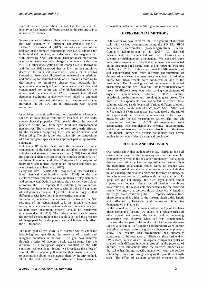
spectral induced polarization method has the potential to
identify and distinguish different species in the subsurface in a non-invasive manner.
Several studies investigated the effect of organic pollutants on
the SIP signature of different contaminants.<sup>10–14</sup>. Schwartz et al. (2012) observed an increase of the
real part of the complex conductivity with NAPL addition for
both diesel and motor oil, and a decrease of the imaginary part
with increasing NAPL saturation. Their proposed mechanism was cation exchange with charged compounds within the
NAPL. Further investigation of the charged NAPL (Schwartz
and Furman 2012) showed that its low surface mobility,
decreased the bulk soil polarization. Blondel et al. (2014) showed that free-phase oil caused an increase of the resistivity
and phase lag for saturated conditions. However, according to
the authors no prominent change was noticeable for
quadrature conductivity (σ") measurements between clean and contaminated nor before and after biodegradation. On the
other hand, Personna et al. (2013) showed that ethanol
depressed quadrature conductivity when added to saturated
sand-clay mixtures and attributed it to suppressed charge movement at the EDL due to interactions with ethanol
molecules.
In addition to organic pollutants, the composition of inorganic species in soils has a well-known influence on the soil's
chemo-physical properties. This greatly affects the use and
practices of the soil, from agricultural and environmental
perspectives. The characteristics of soils are greatly affected by the elements composing their solution (Anderson and
Rubin 1981). Therefore, the need to identify the composition
of these inorganic species is an important part of appropriate
soil usage. Not many IP studies dealt with the influence of ionic
composition of the soil solution and adsorbed species on the
soil electrical signature. Lesmes and Frye (2001) have studied
the pore fluid chemistry effect on the complex conductivity of sandstone. In another work, the SIP signature for adsorption of
hydroxides and mineral precipitation on sand and silica gel
was investigated (Zhang et al. 2012).
Leroy and Revil (2004; 2009) proposed an electrical triple layer chemical complexation model (TLM) to describe
electrochemical properties of clay minerals or clay rich soils
and groundwater. Optimized surface site densities were able to
reproduce the SIP response thus indicating the connection between the Stern layer surface species and the SIP signature
of soil particles such as clays. The literature suggests that
different species have their unique electrical signature.
In order to understand the mechanism controlling the SIP response of the contaminated soil, the possible chemical
interactions between the contaminants and the soil solids (i.e.
as part from adsorption process) should be considered
(Underwood et al. 2015). The surface interactions influence the formed electric field at the double layer and the presence
of charge particles in the pore space, which eventually affect
the SIP response.
The main goal of this study is to examine SIP as a tool for
identifying and quantifying the presence of organic and
inorganic pollutants in the soil. This goal was achieved
through a series of laboratory-scale experiments. First the influence of a free-phase organic pollutant on the SIP
signature was examined. Second, we investigate the effect of
several different organic pollutants and their mixtures, in order
to examine the ability to distinguish them by the SIP method. Third, the soil solution and adsorbed phase inorganic
composition influence on the SIP signature was examined.
EXPERIMENTAL METHODS In this work we have explored the SIP signature of different
soils with various contaminants using the SIP ZEL-SIP04
impedance spectrometer (Forschungszentrum Juelich,
Germany) (Zimmermann et al. 2008). All electrical measurements were conducted with four electrodes in a
Wenner or Schlumberger arrangement. We executed three
main sets of experiments. The first experiment was conducted
on an unsaturated red sandy loam soil in horizontal columns (Shefer et al. 2013). In this experiment the SIP signature of
soil contaminated with three different concentrations of
decane aside a clean treatment were examined. In addition
timely SIP measurements were conducted on one of the treatments. The following set of experiments involved
unsaturated calcium rich Loess soil. SIP measurements were
taken for different treatments with varying combinations of
organic contaminants (decane, TBP, aniline hexadecyltrimethylammonium bromide) in glass boxes. The
third set of experiments was conducted in vertical flow
columns with red sandy loam soil. Various different solutions
that included chloride salts of Ca+2, Na+1, Mg+2, NH4+1 and
K+1 (a single Ba+2 treatment was also conducted at the end of
the experiment) and different combinations of them were
measured with the SIP measurement system. The total salt
concentration was set to 0.01N. All experiments were accompanied with complementary chemical measurements
and in the last two sets the data was also fitted to the Cole-
Cole model. Further, we present preliminary data driven
models for pollutants identification and predication.
RESULTS AND DISCUSSION
Our results show that adding free-phase NAPL to the soil
causes a decrease of the imaginary part of the complex
conductivity as well as the relaxation frequency. We suggest that the polarization mechanism responsible for these results is
the membrane polarization model. Since no change was
observed in solution major ion composition we conclude that
no ion exchange process took place and therefore no change in Stern layer composition. Together with the fact that the soil's
grain size did not change, the Stern layer model cannot
support our findings. Hence, by elimination, membrane
polarization is, the responsible mechanisms for the observed results. We imply that the pore throat characteristic length is
the length scale controlling the SIP response when a free-
phase compound is added to the system, altering this length
and affecting polarization and relaxation time (as demonstrated in Figure 1).
In the second set of experiments, where on top of the free-
phase compound (decane) we added to a calcium-rich soil
other organic compounds, the same trend of decreasing polarization was observed when soil was contaminated.
However, the real part of the conductivity had a clear decrease
(due to a decline in Ca+2 solution concentration) when decane
was added, as opposed to no significant change in the previous study. The calcium rich environment had apparently
contributed to the formation of different surface (mineral or
OM surface) interactions of the organic compounds (polar or
charged with different functional groups) in the presence of decane. These interactions affect the electrical properties of
the soil either through specific interactions with the surface
(Stern layer model) or through changing the pore throat length
scale. The effect of calcium carbonate presence is also

Identifying pollutants with SIP Shefer, Schwartz and Furman
IP2016 – 6-8 June, Aarhus, Denmark 3
considered, as its crystallization might have been encouraged
in the presence of the organic solvents. Due to its insolating nature, it can greatly affect the soil conductivity and
polarization.
In addition, an artificial neural network classification was
presented, that showed a preliminary satisfying ability to indicate the existence of a specific contaminant (see Figure 2).
When examining the SIP method ability to identify and
distinguish inorganic pollutants we see a clear influence of the chemical composition of the soil solution and the adsorbed
phase on the soil's electrical signature. Coherent changes in
the relaxation time and chargeability (or phase values) when
the chemical composition of the soil is changed. Furthermore, we note that divalent cations have a unique influence on the
electrical signature: addition of divalent cation to the porous
media (consisting mainly of monovalent cations) causes an
instantaneous shift in the relaxation frequency, while the polarization magnitude is affected in a more gradual way (see
Figure 3). This raises the idea that perhaps the changes in
relaxation time and in polarization values are independent,
however it should thoroughly examined. Additionally, we have presented three types of data-driven
models to potentially classify the presence or predict the
concentration of inorganic species in the soil, based on the SIP
measurements. The first model was an ANN model that based on the SIP signature of the different treatments can predict the
adsorbed concentrations in the soil. The second model is a
simplified chemical model that enables the prediction of
species mobility, as a first step for their identification. The last model is a linear regression optimization to find the
coefficients which relate the concentrations of species to
chargeability and relaxation time. Even though the models
were based on a limited amount of data, they were able to classify or predict fairly well the concentrations of the primary
soil species.
Figure 3. Phase lag as a function of frequency, for the
second experiment set. Treatments of sodium, sodium-
calcium at 2:1 ratio, sodium- calcium 1:2 ratio
respectively, and calcium (total 0.01N concentration).
CONCLUSIONS The main goal of this study was to examine the ability of the
SIP method to locate and identify pollutants or solution
composition in the soil. A part of this objective was to further
understand the mechanisms responsible for the SIP phenomena of soils. From our work we can draw the
following conclusions:
(1) Membrane polarization model is the dominant mechanism
to explain the findings of free-phase contaminant that are primarily related to the temporal relaxation of pore scale liquid
arrangement. (2) Calcium cations play an important role in
surface interactions with soil mineral and OM in the presence
of hydrocarbons, affecting both membrane and Stern layer polarization mechanisms. (3) Classification of organic
contaminants can be potentially achieved using SIP and data-
driven models. (4) The properties (mobility, valance, radii,
and affinity) of the adsorbed cations affect the electrical signature of the soil. (5) The measured spectra has the
potential to reveal adsorbed concentrations of dominant
species at the solid surface.
REFERENCES
Anderson, N.A. and Rubin, A.J., 1981. Adsorption of
inorganics at solid-liquid interfaces., Ann Arbor Science Publishers, Inc.
Blondel, A. et al., 2014. Temporal evolution of the
geoelectrical response on a hydrocarbon contaminated
site. Journal of Applied Geophysics, 103, pp.161–171. Borner, F.D., Gruhne, M. and Schon, J., 1993. Contamination
Indications Derived From Electrical Properties in the
Low Frequency Range. Geophysical Prospecting, 41,
pp.83–98. Bucker, M. and Hordt, a., 2013. Analytical modelling of
membrane polarization with explicit parametrization of
pore radii and the electrical double layer. Geophysical
Journal International, 194(2), pp.804–813. Jougnot, D. et al., 2010. Spectral induced polarization of
partially saturated clay-rocks: a mechanistic approach.
Geophysical Journal International, 180(1), pp.210–
224. Leroy, P. et al., 2008. Complex conductivity of water-
saturated packs of glass beads. Journal of colloid and
interface science, 321(1), pp.103–17.
Leroy, P. and Revil, a., 2009. A mechanistic model for the spectral induced polarization of clay materials. Journal
of Geophysical Research, 114(B10), p.B10202.
Leroy, P. and Revil, a., 2004. A triple-layer model of the
surface electrochemical properties of clay minerals. Journal of Colloid and Interface Science, 270(2),
pp.371–380.
Lesmes, D.P. and Frye, K.M., 2001. Influence of pore fluid
chemistry on the complex conductivity and induced polarization responses of Berea sandstone. Journal of
Geophysical Research, 106(B3), p.4079.
Marshall, D.J. and Madden, T.R., 1959. INDUCED
POLARIZATION, A STUDY OF ITS CAUSES. GEOPHYSICS, 24(4), pp.790–816.
Olhoeft, G.R., 1985. Low‐ frequency electrical properties.
Geophysics, 50(12), pp.2492–2503.
Personna, Y.R. et al., 2013. Complex resistivity signatures of ethanol biodegradation in porous media. Journal of
Contaminant Hydrology, 153, pp.37–50.
Revil, A. and Florsch, N., 2010. Determination of
permeability from spectral induced polarization in granular media. Geophysical Journal International,
pp.1480–1498.
Revil, A., Schmutz, M. and Batzle, M.L., 2011. Influence of
oil wettability upon spectral induced polarization of oil-bearing sands. Geophysics, 76(5), pp.A31–A36.
Schmutz, M. et al., 2010. Influence of oil saturation upon
spectral induced polarization of oil-bearing sands.
Geophysical Journal International, 183(1), pp.211–224.

Identifying pollutants with SIP Shefer, Schwartz and Furman
IP2016 – 6-8 June, Aarhus, Denmark 4
Schwartz, N. and Furman, A., 2012. Spectral induced
polarization signature of soil contaminated by organic pollutant: Experiment and modeling. Journal of
Geophysical Research: Solid Earth, 117(B10),
Schwartz, N., Huisman, J. a. and Furman, a., 2012. The effect
of NAPL on the electrical properties of unsaturated porous media. Geophysical Journal International,
188(3), pp.1007–1011.
Shefer, I., Schwartz, N. and Furman, a., 2013. The effect of
free-phase NAPL on the spectral induced polarization signature of variably saturated soil. Water Resources
Research, 49(10), pp.6229–6237.
Titov, K. et al., 2002. Theoretical and experimental study of
time domain-induced polarization in water-saturated sands. Journal of Applied Geophysics, 50(4), pp.417–
433.
Titov, K. et al., 2004. through Time Domain Measurements. ,
1168, pp.1160–1168. Underwood, T. et al., 2015. Molecular Dynamic Simulations
of Montmorillonite–Organic Interactions under Varying
Salinity: An Insight into Enhanced Oil Recovery. The
Journal of Physical Chemistry C, 119(13), pp.7282–
7294.
Vanhala, H., Soininen, H. and Kukkonen, I., 1992. Detecting organic chemical contaminants by spectral-induced
polarization method in glacial till environment.
Geophysics, 57(8), pp.1014–1017.
Vaudelet, P. et al., 2011. Changes in induced polarization associated with the sorption of sodium, lead, and zinc
on silica sands. Journal of colloid and interface science,
360(2), pp.739–52.
Zhang, C. et al., 2012. Spectral induced polarization signatures of hydroxide adsorption and mineral precipitation in
porous media. Environmental Science and Technology,
46(8), pp.4357–4364.
Zimmermann, E. et al., 2008. A high-accuracy impedance spectrometer for measuring sediments with low
polarizability. Measurement Science and Technology,
19(10), p.105603.
Figure 1. Solution of the Young-Laplace equation (courtesy of Dr. Leonid Fel) for the described multiphase system, (a) the
clean soil- water air interface (the border of the blue color and white background), before decane was added. (b) after decane
was added : water- decane interface (the border of blue and red colors), and the decane- air interface (border of red color
and white background).
Figure 2. Neural network classification for the binnary presence of the examined pollutants in the soil. Each rectangle
represents a specific conatminant : 0-for not present and 1- present in the soil. Blue dots are for the original measuremnts,
green and red circles are trained and tested data by the ANN respectively. A succesful prediction is indicated by a dot within
a circle. The bottom axis indictaes the type of treatmnent.

IP2016 – 6-8 June, Aarhus, Denmark 1
Doubling the spectrum of time-domain induced polarization: removal of non-linear self-potential drift, harmonic noise and spikes, tapered gating, and uncertainty estimation Per-Ivar Olsson Gianluca Fiandaca Jakob Juul Larsen Torleif Dahlin Esben Auken Engineering Geology Earth Sciences Engineering Engineering Geology Earth Sciences Lund University Aarhus University Aarhus University Lund University Aarhus University Sweden. Denmark Denmark Sweden Denmark [email protected] [email protected] [email protected] [email protected] [email protected]
INTRODUCTION
Recently, the interpretation and inversion of time-domain induced polarization (TDIP) data has changed. Research is moving from only inverting for the integral changeability to also consider the spectral information and inverting for the full induced polarization (IP) response curves. Furthermore, efforts have been made to achieve faster acquisitions and better signal-to-noise ratio (SNR) by using a 100% duty cycle current waveform, without current off-time, for TDIP measurements. However, there still remains drawbacks for the spectral TDIP
measurements, especially its limited spectral information content compared to for example laboratory frequency-domain spectral IP measurements (Revil et al., 2015). To date, only limited work has been done on increasing the spectral information content in TDIP measurement data even though recent developments in TDIP acquisition equipment have enabled access to full waveform recordings of measured potentials and transmitted current (e.g. the Terrameter LS and the Elrec pro). This paper presents a full waveform processing scheme for handling multiple issues limiting the spectral information quality and content. These issues are handled separately starting with background drift removal which is followed by identifying spikes, harmonic denoising, spike removal, tapered gating and uncertainty estimation.
DATA ACQUISITION
To be able to apply the processing scheme described in this paper it is necessary to use an instrument that is capable of recording full waveform data of the measured potentials. The required sampling rate for the full waveform depends mainly on the desired width of the shortest gate, how close it should be to the current switch and avoiding of aliasing. The data presented in this paper were acquired with a 50% duty cycle current waveform and 4s on-time using a Terrameter LS instrument for transmitting current and measuring potentials. The instrument operates at a sampling rate of 30 kHz and applies digital filtering and averaging depending on selected data rate. A data rate of 3750 Hz, corresponding to approximately 0.267 ms per sample, was used for the measurements presented in the paper. The sampling rate was chosen for being able to have the first IP gate one millisecond from the current pulse, considering that earlier gates would certainly suffer from EM-effects which we at present want to avoid, it was not judged meaningful with earlier gates. The instrument input filters were modified with a 4th order Butterworth filter with cutoff frequency of 1.5 kHz to avoid aliasing. Two TDIP profiles (74 meter, 38 electrodes with spacing of two meter) were acquired on a grass field in Aarhus University Campus, with presence of multiple noise sources common in urban environments. The profiles were acquired with the instrument and settings as described in the previous paragraph, a multiple gradient protocol (364 quadrupoles) and acid-grade stainless steel electrodes.
IP GATE DISTRIBUTION For retrieving spectral information close to the current pulses there is a need for gates which are shorter than the time-period of the harmonic noise (i.e. shorter than 20 ms for 50 Hz). This
SUMMARY This paper presents an advanced signal processing scheme for time-domain induced polarization full waveform data. The scheme includes several steps with an improved induced polarization (IP) response gating design using convolution with tapered windows to suppress high frequency noise, a logarithmic gate width distribution for optimizing IP data quality and an estimate of gating uncertainty. Additional steps include modelling and cancelling of non-linear background drift and harmonic noise and a technique for efficiently identifying and removing spikes. The cancelling of non-linear background drift is based on a Cole-Cole model which effectively handles current induced electrode polarization drift. The model-based cancelling of harmonic noise reconstructs the harmonic noise as a sum of harmonic signals with a common fundamental frequency. After segmentation of the signal and determining of noise model parameters for each segment, a full harmonic noise model is subtracted. Furthermore, the uncertainty of the background drift removal is estimated which together with the gating uncertainty estimate and a uniform uncertainty gives a total, data-driven, error estimate for each IP gate. The processing steps is successfully applied on full field profile data sets. With the model-based cancelling of harmonic noise, the first usable IP gate is moved one decade closer to time zero. Furthermore, with a Cole-Cole background drift model the shape of the response at late times is accurately retrieved. In total, this processing scheme achieves almost four decades in time and thus doubles the available spectral information content of the IP responses compared to the traditional processing. Key words: Spectral induced polarization; Time-domain; Signal processing; Uncertainty estimate; Electrical properties;
Doubling the spectrum of time-domain induced polarization Olsson et al.
IP2016 – 6-8 June, Aarhus, Denmark 2
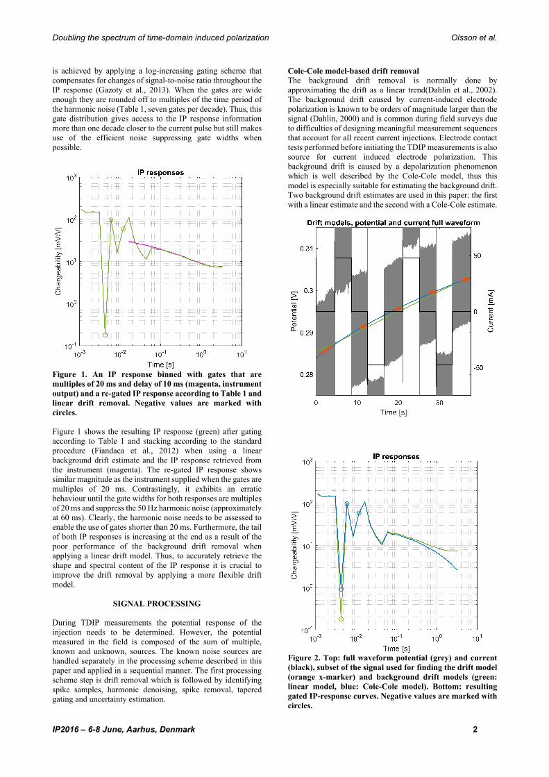
is achieved by applying a log-increasing gating scheme that compensates for changes of signal-to-noise ratio throughout the IP response (Gazoty et al., 2013). When the gates are wide enough they are rounded off to multiples of the time period of the harmonic noise (Table 1, seven gates per decade). Thus, this gate distribution gives access to the IP response information more than one decade closer to the current pulse but still makes use of the efficient noise suppressing gate widths when possible.
Figure 1. An IP response binned with gates that are multiples of 20 ms and delay of 10 ms (magenta, instrument output) and a re-gated IP response according to Table 1 and linear drift removal. Negative values are marked with circles. Figure 1 shows the resulting IP response (green) after gating according to Table 1 and stacking according to the standard procedure (Fiandaca et al., 2012) when using a linear background drift estimate and the IP response retrieved from the instrument (magenta). The re-gated IP response shows similar magnitude as the instrument supplied when the gates are multiples of 20 ms. Contrastingly, it exhibits an erratic behaviour until the gate widths for both responses are multiples of 20 ms and suppress the 50 Hz harmonic noise (approximately at 60 ms). Clearly, the harmonic noise needs to be assessed to enable the use of gates shorter than 20 ms. Furthermore, the tail of both IP responses is increasing at the end as a result of the poor performance of the background drift removal when applying a linear drift model. Thus, to accurately retrieve the shape and spectral content of the IP response it is crucial to improve the drift removal by applying a more flexible drift model.
SIGNAL PROCESSING
During TDIP measurements the potential response of the injection needs to be determined. However, the potential measured in the field is composed of the sum of multiple, known and unknown, sources. The known noise sources are handled separately in the processing scheme described in this paper and applied in a sequential manner. The first processing scheme step is drift removal which is followed by identifying spike samples, harmonic denoising, spike removal, tapered gating and uncertainty estimation.
Cole-Cole model-based drift removal The background drift removal is normally done by approximating the drift as a linear trend(Dahlin et al., 2002). The background drift caused by current-induced electrode polarization is known to be orders of magnitude larger than the signal (Dahlin, 2000) and is common during field surveys due to difficulties of designing meaningful measurement sequences that account for all recent current injections. Electrode contact tests performed before initiating the TDIP measurements is also source for current induced electrode polarization. This background drift is caused by a depolarization phenomenon which is well described by the Cole-Cole model, thus this model is especially suitable for estimating the background drift. Two background drift estimates are used in this paper: the first with a linear estimate and the second with a Cole-Cole estimate.
Figure 2. Top: full waveform potential (grey) and current (black), subset of the signal used for finding the drift model (orange x-marker) and background drift models (green: linear model, blue: Cole-Cole model). Bottom: resulting gated IP-response curves. Negative values are marked with circles.

Doubling the spectrum of time-domain induced polarization Olsson et al.
IP2016 – 6-8 June, Aarhus, Denmark 3
To reduce the risk of any harmonic noise or IP response interfering with the drift model data, the fit is conducted for a subset of a down-sampled signal, taken at the end of the off-time period for the 50% duty-cycle and on-time period if applying a 100% duty-cycle current waveform. Fig. 2 show examples of generated drift models, as well as the resulting IP responses after gating and stacking the signal. Clearly, the linear model is not sufficient for accurately describing the drift in the full waveform potential and as a result it gives unrealistic increasing chargeability values for late gates of the IP response. Contrastingly, the Cole-Cole model shows a good fit to drift data and consequently the resulting IP response does not exhibit the erroneous behavior at late gates. In total, it is clear that a linear drift model gives incorrect IP responses, especially at late times when signal-to-noise ratio is smaller and that a more advanced drift model such as the Cole-Cole is needed. Model-based cancelling of harmonic noise The processing approach applied in this paper is similar to the processing successfully applied on data from other geophysical methods, for example magnetic resonance soundings (Larsen et al., 2013) and seismoelectrics (Butler and Russell, 1993) but it has in this case been adapted to be applicable for data from TDIP measurement. The method takes a model-based approach for processing the TDIP full waveform potential by describing the harmonic noise in terms of a sum of harmonic signals. The different harmonic signals have frequencies given by a common fundamental frequency (f0) multiplied with an integer (m) to describe the different harmonics but have independent amplitudes (αm and βm) for each harmonic m:
cos 2 sin 2
for sample index n and sampling frequency fs. The reader is referred to the mentioned references for details. Removal of full waveform spikes Despiking of the measured full waveform signal is done for two main reasons. The first reason is that spikes in the full waveform data can corrupt the integrated values for IP gates, especially for short gates consisting of a few samples when only part of the spike falls within the gate thus having large effect on the integrated value. The second reason is related to the modelling of the harmonic noise and how the finding of noise model parameters is implemented in this paper which is known to be sensitive to spikes in data (Larsen et al., 2013). The method for finding the spikes used in this paper employs several steps to enhance the spikes in the signal and defines a data-driven, automatic threshold limit based on a Hampel filter (Pearson, 2002) to determine if a sample index is to be considered as spike or not. By applying the filters in this manner an automatic data-driven threshold variable along the full-waveform acquisition is defined. All the samples above the threshold are marked as spikes and are neglected when performing the calculations for the residual energy in the harmonic denoising procedure. After harmonic denoising are the spike sample values replaces by the mean of their non-spike neighbours in the denoised signal. Tapered gate design and error estimation Today, the standard procedure for gating IP is to average the data within the predefined IP gates, corresponding to a discrete and normalized convolution with a rectangular window. In other geophysical methods (e.g. electromagnetic) a gate method applying different kinds of tapered windows have been used since decades (Macnae et al., 1984). Tapered window functions are superior in suppressing high frequency noise compared to
the rectangular counterpart. Furthermore, the tapered windows allow the use of wider gates which has higher noise suppression, without distorting the signal. I this paper, a Gaussian window with 3.5 times the width of the traditional rectangular window width was applied before evaluating the IP gate values. With this window, the main frequency response lobe of both windows cuts at approximately the same normalized frequency but the side lobes of the Gaussian window have around 40 dB higher frequency suppression. Uncertainty estimation of the data for individual IP gates cannot be retrieved by directly comparing the individual IP stacks because each individual stack is different due to superposition from previous pulses (Fiandaca et al., 2012), hence other approaches are needed. It is also desirable that an uncertainty estimate make use of the advantage of applying the convolution with tapered gates as described in this paper. If enough gates per decade are used for gating the data, the signal variability is almost linear within the gates and for IP signals the linearity is more evident in lin-log space. Thus, it is possible to use a linear fit of the convoluted gate in lin-log space for estimating the gate uncertainty by taking the difference between the fit and the convoluted gate data. The difference gives a measure of the noise content within the gate after the convolution.
FULL FIELD PROFILE PROCESSING EXAMPLE
The processing scheme presented in this paper has been successfully applied to the entire test datasets with substantial improvements in spectral information content, data reliability and quality. One of the datasets is presented here as an illustration. Figure 4 shows IP responses from instrument processing and the redesigned processing scheme presented by this paper. The spurious IP increase present at late times in the response retrieved by the instrument is removed in the reprocessed IP response as a result of the improved drift removal. At the same time, the harmonic denoising processing enables to retrieve reliable IP data already 2.2 ms after the current switch, one decade closer to time zero compared to instrument IP processing.
Figure 4. IP responses from instrument processing (magenta, instrument output) and the redesigned processing scheme presented by this paper (light blue) with error bars corresponding to one STD. Gates rejected by processing for containing spikes are marked in grey.

Doubling the spectrum of time-domain induced polarization Olsson et al.
IP2016 – 6-8 June, Aarhus, Denmark 4
Figure 5 shows pseudosections for a full data set acquired on the same profile as the previous data example was extracted from. It shows gates for IP responses generated by the full signal processing routine and corresponding pseudosections for the same gates but only applying the linear background drift removal. For the early gates which are not a multiple of the time period of the harmonic noise there is a clear improvement with much smoother pseudosection from gate 3 and higher. Contrastingly, IP gate number 18 which is little affected by the background drift removal shows very similar pseudosections for the two processing examples. However, the pseudosections for the last IP gate (25) show some difference due to the sensitivity of the late gates for background drift estimates where the linear drift model sometimes causes the IP responses to increase at late times. Again, the improved processing with Cole-Cole drift estimate shows smoother variation in the pseudosection, especially on the left side.
Figure 5. Pseudosections for IP gates 3, 9, 18 and 25 (from top-down) for processed data without harmonic denoising and linear drift removal (left) and with harmonic denoising and Cole-Cole drift removal (right) of full waveform data.
CONCLUSIONS
The TDIP signal processing scheme described in this paper significantly improves the handling of background drift, spikes and harmonic noise superimposed on the potential response in the measured full waveform potential. The Cole-Cole background drift removal substantially increases the accuracy of the drift model for non-linear drift cases and recovers the shape of the IP response at late times. The reliability of early IP response times, down to a few ms, is generally increased with a flexible data-driven despiking algorithm and model-based harmonic denoising. Furthermore, the improved gate distribution and tapered design gives access to early spectral IP response information and overall increases the signal-to-noise ratio by applying tapered and overlapped gates without distorting the IP response. Additionally, the data driven uncertainty estimates of the individual IP gate values provides valuable information for assessing data quality and for succeeding spectral inversion. In total, this processing moves the first gate one decade closer to time zero, recovers the late gates with reduced bias and supplies valuable estimates of IP gate uncertainty. These improvements double the usable spectral information of the IP response, achieving almost four decades in time, compared to instrument processing procedure.
ACKNOWLEDGMENTS
Funding for the work was provided by Formas - The Swedish Research Council for Environment, Agricultural Sciences and Spatial Planning, (ref. 2012-1931), BeFo - Swedish Rock Engineering Research Foundation, (ref. 331) and SBUF - The Development Fund of the Swedish Construction Industry, (ref. 12719). The project is part of the Geoinfra-TRUST framework (Transparent Underground Structure, http://www.trust-geoinfra.se/). Further support was provided by the research project GEOCON, Advancing GEOlogical, geophysical and CONtaminant monitoring technologies for contaminated site investigation (contract 1305-00004B). The funding for GEOCON is provided by The Danish Council for Strategic Research under the Programme commision on sustainable energy and environment. Finally, additional funding was provided by Hakon Hansson foundation (ref. HH2015-0074) and Ernhold Lundström foundation.
REFERENCES
Butler, K.E., Russell, R.D., 1993. Subtraction of powerline harmonics from geophysical records. Geophysics 58, 898. doi:10.1190/1.1443474
Dahlin, T., 2000. Short note on electrode charge-up effects in DC resistivity data acquisition using multi-electrode arrays. Geophysical Prospecting 48, 181–187. doi:10.1046/j.1365-2478.2000.00172.x
Dahlin, T., Leroux, V., Nissen, J., 2002. Measuring techniques in induced polarisation imaging. Journal of Applied Geophysics 50, 279–298. doi:10.1016/S0926-9851(02)00148-9
Fiandaca, G., Auken, E., Christiansen, A.V., Gazoty, A., 2012. Time-domain-induced polarization: Full-decay forward modeling and 1D laterally constrained inversion of Cole-Cole parameters. Geophysics 77, E213–E225. doi:10.1190/geo2011-0217.1
Gazoty, A., Fiandaca, G., Pedersen, J., Auken, E., Christiansen, A. V, 2013. Data repeatability and acquisition techniques for time-domain spectral induced polarization. Near Surface Geophysics 391–406. doi:10.3997/1873-0604.2013013
Larsen, J.J., Dalgaard, E., Auken, E., 2013. Noise cancelling of MRS signals combining model-based removal of powerline harmonics and multichannel Wiener filtering. Geophysical Journal International 196, 828–836. doi:10.1093/gji/ggt422
Macnae, J.C., Lamontagne, Y., West, G.F., 1984. Noise processing techniques for time-domain EM systems. Geophysics 49, 934–948. doi:10.1190/1.1441739
Pearson, R.K., 2002. Outliers in process modeling and identification. IEEE Transactions on Control Systems Technology 10, 55–63. doi:10.1109/87.974338
Revil, A., Binley, A., Mejus, L., Kessouri, P., 2015. Predicting permeability from the characteristic relaxation time and intrinsic formation factor of complex conductivity spectra. Water Resources Research 51, 6672–6700. doi:10.1002/2015WR017074
Table 1. Duration of delay time and IP gates for the processed field data corresponding to seven gates per decade. Note that the width of the gates from 13 and higher are multiples of 20 ms.
Gate number Delay 1 2 3 4 5 6 7 8 9 10 11 12 Width [ms] 1 0.26 0.53 0.80 1.06 1.33 2.13 2.93 4 5.33 7.46 10.4 14.4 Gate number 13 14 15 16 17 18 19 20 21 22 23 24 25 Width [ms] 20 20 40 60 60 120 120 180 300 360 540 780 1020
IP2016 – 6-8 June, Aarhus, Denmark 1
An analysis of Cole-Cole parameters for IP data using Markov chain Monte Carlo L. M. Madsen, C. Kirkegaard, G. Fiandaca, A. V. Christiansen, and E. Auken University of Aarhus, HydroGeophysics Group, Institute for Geoscience C. F. Møllers Alle 4, DK-8000 Aarhus C, Denmark Correspondence to: L. M. Madsen ([email protected])
INTRODUCTION
Recently, the interpretation and inversion of TDIP data has
changed from only inverting for the integral changeability to
also consider the spectral information contained in the IP
response curves (Fiandaca et al., 2012, 2013). Several
examples of spectral TDIP applications have been presented,
for landfill delineation (Gazoty et al., 2012b, 2013), lithotype
characterization (Chongo et al., 2015; Gazoty et al., 2012a;
Johansson et al., 2015), time-lapse monitoring of CO2
injection (Doetsch et al., 2015a; Fiandaca et al., 2015) and
freezing of active layer in permafrost (Doetsch et al., 2015b).
Furthermore, efforts have been made to achieve a wider time-
range in TDIP acquisition, up to four decades in time (Olsson
et al., 2016), for enhanced spectral content.
The spectral inversion of TDIP data is a high dimensional
nonlinear problem. Ghorbani et al. (2007) argued that the
problem is too nonlinear to be solved with least-squares
methods, and that Cole-Cole parameters cannot be resolved
from TDIP data.
The aim of this study is to analyse the uncertainty and
correlation of spectral Cole-Cole parameters retrieved from
TDIP data. This is done using the Markov chain Monte Carlo
(MCMC) method with a novel model proposer.
MCMC ALGORITHM
A new MCMC algorithm is developed to sample the posterior
probability distribution of the model space of the Cole-Cole
parameters (Pelton et al., 1978) for the 1D TDIP forward
mapping described in Fiandaca et al. (2012):
(1)
Where ρj is the DC resistivity and m0,j, τj, and Cj are the IP
parameters of the j’th layer with thickness thkj.
The Markov chain follows a random walk through the model
space, where the next model in the chain only depends on the
current model. Our MCMC algorithm is based on the
Metropolis-Hastings sampling algorithm, which includes the
following two steps (Metropolis et al., 1953; Hasting 1970):
(1) A new model (mnew) is proposed from a proposal
distribution q(mnew|mc), where mc is the current model. The
model proposer used here is introduced in the next section.
(2) The proposed model is accepted or rejected based on an
acceptance criterion, which is also described later.
These two steps are repeated to generate a Markov Chain of
models.
Model proposer
The computations are carried out in a logarithmic space to
enhance linearity, with the model vector defined by:
m = log(ρi), log(m0,i), log(τi), log(Ci), log(thkj);
i=1:Nlayers; j=1:Nlayers-1
(2)
Where ρ is the resistivity [Ωm], m0 is the chargeability
[mV/V], τ is the time constant [sec], C is the dimensionless
frequency exponent, and thk is the layer thickness [m].
SUMMARY
The Markov chain Monte Carlo (MCMC) method is used
to invert time-domain induced polarization (TDIP) data.
A novel random-walk algorithm samples models from a
probability distribution based on a realisation of the
model covariance matrix, allowing the algorithm to vary
step lengths according to parameter uncertainty. The
algorithm was found to converge to the posterior
distribution over one hundred times faster than a standard
Gaussian distributed model proposer.
Synthetic TDIP data, simulating homogenous half spaces
and three-layer models, are inverted using the MCMC
method. The results show bell-shaped posterior
distributions for all spectral Cole-Cole parameters with
clear correlations between the parameters.
Small values of the frequency exponent (C) are found to
decrease the resolution of the model parameters. A
comparative analysis between the standard deviations of
the MCMC posterior distributions and the results of a
linearized inversion shows that the linearized approach
works well with well-resolved model parameters.
We have compared inversion results of different
acquisition times and current waveforms. We found that
as the time range decreases the parameter correlations
become nonlinear and the parameters become poorly
resolved or completely unresolved.
Combined, the inversion results show that it is possible to
extract the spectral Cole-Cole parameters from time-
domain IP data and that a linearized approach is justified
for a sufficient acquisition range.
Key words: Time-domain induced polarization, Inverse
theory, Markov chain Monte Carlo, Electric properties,
Hydrogeophysics.

MCMC analysis of TDIP data Madsen et al.
IP2016 – 6-8 June, Aarhus, Denmark 2
The new model, mnew, is drawn from a normal distribution.
The new proposed model is defined by:
mnew = mc + Δ (3)
Where mc and Δ are the current model and the perturbation in
the Markov chain, with Δ computed as:
Δ = L ·n ·k (4)
The vector n contains random numbers drawn from a normal
distribution and the constant k is the step length. L is the
Cholesky decomposition of the linearized covariance matrix
Cest of the initial model:
Cest= LLT (5)
This realisation of the model covariance matrix allows the
proposer to take larger steps for poorly defined parameters.
This makes the Markov chain convergence faster towards the
target distribution. The covariance matrix, Cest, is defined as in
Auken et al. (2005).
The step length is adjusted for each Markov chain, so that the
acceptance rate of new models is approximately 20-35%. A
value of five is chosen as a maximum for the perturbation in
order to confine the distance between mnew and mc.
Model acceptance criterion
The next step of the Metropolis-Hastings algorithm is to
determine whether a proposed model should be accepted or
rejected. If mnew is accepted, the model becomes the next
model mc in the Markov chain. If P(m) is the probability
distribution of the model m, then the acceptance probability of
the new model is given by:
(6)
As the proposal distribution is symmetric in the logarithmic
space, the equation reduces to:
(7) (6)
So, the model mnew is always accepted if its probability is
larger than the probability of the current model. If its
probability is smaller, then the model is accepted with
probability α.
SYNTETIC DATA
Given a layered medium described by the Cole-Cole model,
the 1D forward TDIP response is calculated using the
algorithm presented by Fiandaca et al. (2012).
Single quadrupolar measurements (geometric factor of
approximately 470 m) and Schlumberger soundings (20
quadrupoles) are simulated for homogenous half spaces and
three-layer models, respectively. The Cole-Cole parameters
range between ρ = 10 - 1000 Ωm, m0 = 5 - 800 mV/V, τ =
0.001 - 10 sec and C = 0.1 - 0.6. Three stacks are considered
for each quadrupole, with both 50% duty cycle and 100% duty
cycle waveforms (Olsson et al., 2015). Two different
distributions of gates are used to simulate varying acquisition
range. The minimum range has 20 gates generated with
increasing widths of 20-200 msec, a current on-time of 2 sec
and a measurement delay of 20 msec as used by Ghorbani et
al. (2007). The maximum range has 22 gates generated with
approximately log-distributed widths from 1.06 to 1300 sec.
The on- and off-time of the current is 4 sec, and the
measurement delay is 2.59 msec.
A Gaussian noise model is added to resistivity and
chargeability values with a standard deviation equal to 2% for
the resistivity and 10% for the chargeability. Additional a
voltage threshold of 0.01 V is added to the data. The noise is
added to give the best simulation of the noise level in the field
(Gazoty et al., 2013).
In the following the results of a homogenous half space with
model parameters ρ = 100 Ωm, m0 = 200 mV/V, τ = 0.01 sec,
C = 0.6 and a maximum acquisition range with 50% duty
cycle is presented as an example.
CONVERGENCE
We have tested the convergence of the covariance-scaled
MCMC model proposer in comparison to the basic Gaussian
model proposer. For the Gaussian proposer Eq. (4) reduces to:
Δ = n ·k (8) (7)
It is found that the covariance-scaled proposer and the
Gaussian proposer find approximately the same posterior
model distribution (Figure 1), but the covariance-scaled
proposer convergences towards the target distribution much
faster. For the previous defined homogenous half space, the
proposers analyse 5.000 and > 500.000 models, respectively,
before reaching convergence. Using the scaled model
proposer reduces the computation time for simple models
from approximate one hour to 20 sec on 10 cores.
Figure 1: The normalised posterior distributions of Cole-
Cole parameter τ resulting from two different model
proposers: A covariance-scaled proposer (A) and a
Gaussian proposer (B). The figure illustrates the faster
convergence rate of the covariance-scaled model proposer,
where we see convergence after just 5000 model proposes.
RESULTS

MCMC analysis of TDIP data Madsen et al.
IP2016 – 6-8 June, Aarhus, Denmark 3
Figure 2 (last page) shows the posterior distribution of the DC
resistivity and the IP parameters for the homogeneous half
space defined earlier. 100,000 models are proposed and 33 %
are accepted and added to the posterior distribution. The
histograms along the diagonal show the distributions of
parameter values in log space with the true model values
indicated in red. The off-diagonal are cross-plots of all
combinations of the four parameters.
The distributions are all bell-shaped, which means they are all
approximately log-normal. The parameters show a single
maximum and are resolved to a different extent. However
skewness is evident for m0 and τ.
The DC resistivity is almost uncorrelated to the Cole-Cole
parameters. The chargeability shows a negative correlation to
τ and C with a Person’s correlation coefficient of 0.77 and
0.70 respectively. The correlation between to τ and C is
positive with a correlation coefficient of 0.86.
It is possible to compute the standard deviation (STD) on the
model parameters from the posterior distributions. A relative
standard deviation factor (STDF) is used here, where the 68%
confidence interval for parameter p then lies between:
(9)
A perfect resolution will give STDF = 1. Using the
terminology from Auken et al., (2005), STDF < 1.2 is a well-
resolved parameter, 1.2 < STDF < 1.5 is a moderately
resolved parameter, 1.5 < STDF < 2 is a poorly resolved
parameter and STDF > 2 is an unresolved parameter. For the
MCMC posterior distribution the standard deviation is
calculated over all accepted models.
The STDF values are shown in Figure 3 for a varying value of
the frequency exponent C. Together with the MCMC STDFs,
we show the STDFs obtained from the linearized approach.
Figure 3 shows that the uncertainty increases if the value of C
is decreased. This holds for both the MCMC- and the
linearized approach. For C = 0.6 all parameters, except τ, is
well resolved with STDF < 1.2 for both MCMC- and
linearized inversion. For C = 0.2, only the resistivity value is
well resolved. The linearized estimations of the STDFs are
reasonable for well resolved parameters, but are
underestimated for poorly resolved parameters. As the C-
value decreases the posterior distribution of the Cole-Cole
parameters resulting from the MCMC analysis become more
non-loglinear and the correlation between the model
parameters becomes stronger.
More complex three-layer models verify the results with
resolved bell-shaped posterior distributions for all the Cole-
Cole parameters and linear correlations. Synthetic data are
simulated on the same homogenous half space with a
minimum acquisition range. The MCMC result shows nearly
bell-shaped posterior distributions, but with nonlinear
correlations between the parameter C and m0 and between C
and tau. The STDFs of the DC resistivity and C are almost
unchanged compared to the result of the maximum range, but
τ and m0 are unresolved. The maximum of the posterior
distribution and the true model is not consistent as well.
Similar results are obtained for the 100% duty cycle data,
confirming the equivalence of the 50% and 100% duty cycle
waveforms for spectral resolution.
Figure 3: Standard deviation factor (STDF) as a function
of the Cole-Cole parameter C. The STDF is computed for
the results of a linearized approach and the MCMC
results. NB: If the STDF value is above 5, it is put to 5.
CONCLUSIONS
The results of running a MCMC inversion of synthetic TDIP
data show that it is possible to extract the spectral Cole-Cole
parameters from time-domain data.
The sampled posterior probability distributions of the Cole-
Cole parameters are all bell-shaped with one maximum.
Strong correlations are present between the IP parameters and
for more complex models correlations can also been seen
between these and the DC resistivity.
The uncertainties of the model parameters increase with
decreasing values of C, which makes it more difficult to
resolve parameters. This holds for the MCMC and the
linearized approach. However the linearized standard
deviations work well for well resolved parameters.
If the acquisition range is too short (2 decades or less), then
the Cole-Cole parameters become poorly- or completely
unresolved, and the correlations become nonlinear.
In general, all the results justify the linearized inversion of
TDIP data for resolved Cole-Cole parameters, when the
necessary acquisition range is used.
REFERENCES
Auken, E., A. V. Christiansen, B. H. Jacobsen, N. Foged, and
K. I. Sørensen, 2005, Piecewise 1D laterally constrained
inversion of resistivity data: Geophysical Prospecting, 53,
497–506.
Chongo M., Christiansen A.V., Fiandaca G., Nyambe I.A.,
Larsen F. & Bauer-Gottwein P., 2015. Mapping localised
freshwater anomalies in the brackish paleo-lake sediments of
the Machile-Zambezi Basin with transient electromagnetic
sounding, geoelectrical imaging and induced polarisation,
Journal of Applied Geophysics, 123, 81-92.
10.1016/j.jappgeo.2015.10.002.
Doetsch J., Ingeman-Nielsen T., Christiansen A.V., Fiandaca
G., Auken E. & Elberling B., 2015a. Direct current (DC)
resistivity and induced polarization (IP) monitoring of active

MCMC analysis of TDIP data Madsen et al.
IP2016 – 6-8 June, Aarhus, Denmark 4
layer dynamics at high temporal resolution, Cold Regions
Science and Technology, 119, 16-28.
10.1016/j.coldregions.2015.07.002.
Doetsch J., Fiandaca G., Auken E., Christiansen A.V., Cahill
A.G. & Jakobsen R., 2015b. Field-scale time-domain spectral
induced polarization monitoring of geochemical changes
induced by injected CO2 in a shallow aquifer, Geophysics, 80,
WA113-WA126. 10.1190/geo2014-0315.1.
Fiandaca, G., Auken, E., Christiansen, A. V. and Gazoty, A.,
2012, Time-domain-induced polarization: Full-decay forward
modelling and 1D laterally constrained inversion of Cole-Cole
parameters: Geophysics, 77, 3, E213-E225.
Fiandaca G., Ramm J., Binley A., Gazoty A., Christiansen
A.V. & Auken E., 2013. Resolving spectral information from
time domain induced polarization data through 2-D inversion,
Geophysical Journal International, 192, 631-646.
10.1093/gji/ggs060.
Fiandaca G., Doetsch J., Vignoli G. & Auken E., 2015a.
Generalized focusing of time-lapse changes with applications
to direct current and time-domain induced polarization
inversions, Geophysical Journal International, 203, 1101-
1112. 10.1093/gji/ggv350.
Gazoty A., Fiandaca G., Pedersen J., Auken E., Christiansen
A.V. & Pedersen J.K., 2012a. Application of time domain
induced polarization to the mapping of lithotypes in a landfill
site, Hydrology and Earth System Sciences, 16, 1793-1804.
10.5194/hess-16-1793-2012.
Gazoty, A., Fiandaca, G., Pedersen, J., Auken, E. and
Christiansen, A. V., 2012b. Mapping of landfills using time-
domain spectral induced polarization data: the Eskelund case
study: Near Surface Geophysics, 10, 575-586.
Gazoty A., Fiandaca G., Pedersen J., Auken E. and
Christiansen A.V., 2013. Data repeatability and acquisition
techniques for time-domain spectral induced polarization:
Near Surface Geophysics, 11, 391-406.
Ghorbani, A., C. Camerlynck, N. Florsch, P. Cosenza, and A.
Revil, 2007, Bayesian inference of the Cole-Cole parameters
from time- and frequency-domain induced polarization:
Geophysical Prospecting, 55, 589–605.
Johansson S., Fiandaca G. & Dahlin T., 2015. Influence of
non-aqueous phase liquid configuration on induced
polarization parameters: Conceptual models applied to a time-
domain field case study, Journal of Applied Geophysics, 123,
295-309. 10.1016/j.jappgeo.2015.08.010.
Olsson P.I., Fiandaca G., Larsen J.J., Dahlin T., Auken E.,
2016. Doubling the spectrum of time-domain induced
polarization: removal of non-linear self-potential drift,
harmonic noise and spikes, tapered gating, and uncertainty
estimation. 4th IP Workshop, 6-8 June 2016, Aarhus,
Denmark.
Olsson, P.-I., Dahlin, T., Fiandaca, G., and Auken E., 2015.
Measuring time-domain spectral induced polarization in the
on-time: decreasing acquisition time and increasing signal-to-
noise ratio, Journal of Applied Geophysics, 123, 316-321.
10.1016/j.jappgeo.2015.08.009.
Hastings, w. K., 1970, Monte Carlo sampling method using
Markov Chains and their appllications: Biometrika, 57, 97-
109.
Pelton, W. H., S. H. Ward, P. G. Hallof, W. R. Sill, and P. H.
Nelson, 1978, Mineral discrimination and removal of
inductive coupling with multifrequency IP: Geophysics, 43,
588–609.
Metropolis, N., Rosenbulth, A., Rosenbulth, M., Teller, A.
and Teller, E., 1953, equation of state calculations by fast
computing machines: Journal of Chemical Physics, 21, 1087-
1092.
Figure 2: The posterior probability distribution of the Cole-Cole parameters for a homogenous half space: ρ = 100 Ωm, m0 =
200 mV/V, τ = 0.01 sec, C = 0.6. The diagonal shows histograms of the distribution of each Cole-Cole parameter. The off-
diagonal shows the correlation between the parameters. The true model parameters are indicated in red. Note the figure is
symmetric about the diagonal.

IP2016 – 6-8 June, Aarhus, Denmark 1
Simulation of membrane polarization for 2D and 3D pore networks Hermann Stebner Andreas Hördt TU Braunschweig TU Braunschweig
Mendelssohnstr. 3 Mendelssohnstr. 3
38106 Braunschweig 38106 Braunschweig
[email protected] [email protected]
INTRODUCTION
The characterization of porous media (e.g. unconsolidated
sediment or rocks) by geophysical methods is a research topic
of fundamental importance in environmental and economic
issues like the investigation of water reservoirs or the
evaluation of waste deposits. The spectral induced polarization
(SIP) method is supposed to have big potential to provide
useful information based on relationships between electric and
hydraulic parameters.
Several empirical approaches for the interpretation of the
measured SIP response exist. Attempts have been made to
correlate a characteristic time scale, derived from the phase-
shift spectra, with measured material parameters like hydraulic
conductivity or pore radii (Titov et al., 2010; Binley et al.,
2005). Another approach is to compare the imaginary
conductivity at a single frequency (Weller et al., 2010) to the
specific surface of the pore space. Although both methods are
based on different assumptions they are supported by
examples of reasonable agreement with laboratory
experiments.
The formulation of a comprehensive theoretical model is
difficult because the underlying physical processes on the pore
scale are not yet fully understood. The two main models, the
theory of electrochemical polarization, first suggested by
Schwarz (1962), and subsequently extended by several authors
(e.g. Leroy et al. 2008; Revil and Florsch 2010), and the theory
of membrane polarization, first suggested by Marshall and
Madden (1959) and extended by Bücker and Hördt (2013), are
both based on the ion movement in the electrical double layer.
The fundamental difference between the both models is
expressed in the definition of the mineral geometry. The
electrochemical polarization is based on mineral grains where
the polarization effect is based on a local concentration of
charge on the grain. The membrane polarization is based on
sequences of narrow and wide pores where the polarization
effect is caused by narrow throats between the pores (FIGURE
1).
Figure 1: Marshall and Madden polarization. Overlapping
cation layers in pore throats (grey) lead to decreased anion
mobility. An applied electric field causes concentration
gradients which relax with a characteristic time after
switch-off.
While the original membrane polarization model was (besides
the pore fluid properties) primarily parametrized by pore
lengths and differing ion mobilities, the expansion by Bücker
and Hördt (2013) introduced a parametrization by pore radii
instead of ion mobilities. This allowed to describe the pore
geometry by a sequence of narrow and wide cylinders
(FIGURE 2). With subsequent development on the electrolyte
parametrization and on the pH, salinity and temperature
dependence the model had some success in reproducing
features also observed with experimental data (e.g. Hördt et al.
2016a; Bairlein et al. 2016).
Figure 2: 2D-extension of the model. Parameterizing the
narrow and wide pores through pore radii allows to
SUMMARY
We extend an existing membrane polarization model to
2D and 3D pore combinations networks, which are
numerically solved to obtain an overall SIP response. We
investigate the behaviour of these networks by varying
the distribution function of the pore combinations and the
size of the network.
Equally distributed pore combinations show a dominance
of high phase shifts. For empirically distributed
combinations, obtained from measured pore radii
distributions, high phase shifts tend to dominate only in
big 3D networks. Our simulations show that for networks,
which are comparable to real rocks, higher maximum
phase shifts than the mean of the original pore
combinations are possible. The results suggest that
networks may allow a simulation of more realistic pore
geometries than the original 2-pore system.
Key words: membrane polarization, pore networks,
measured pore radii distribution.
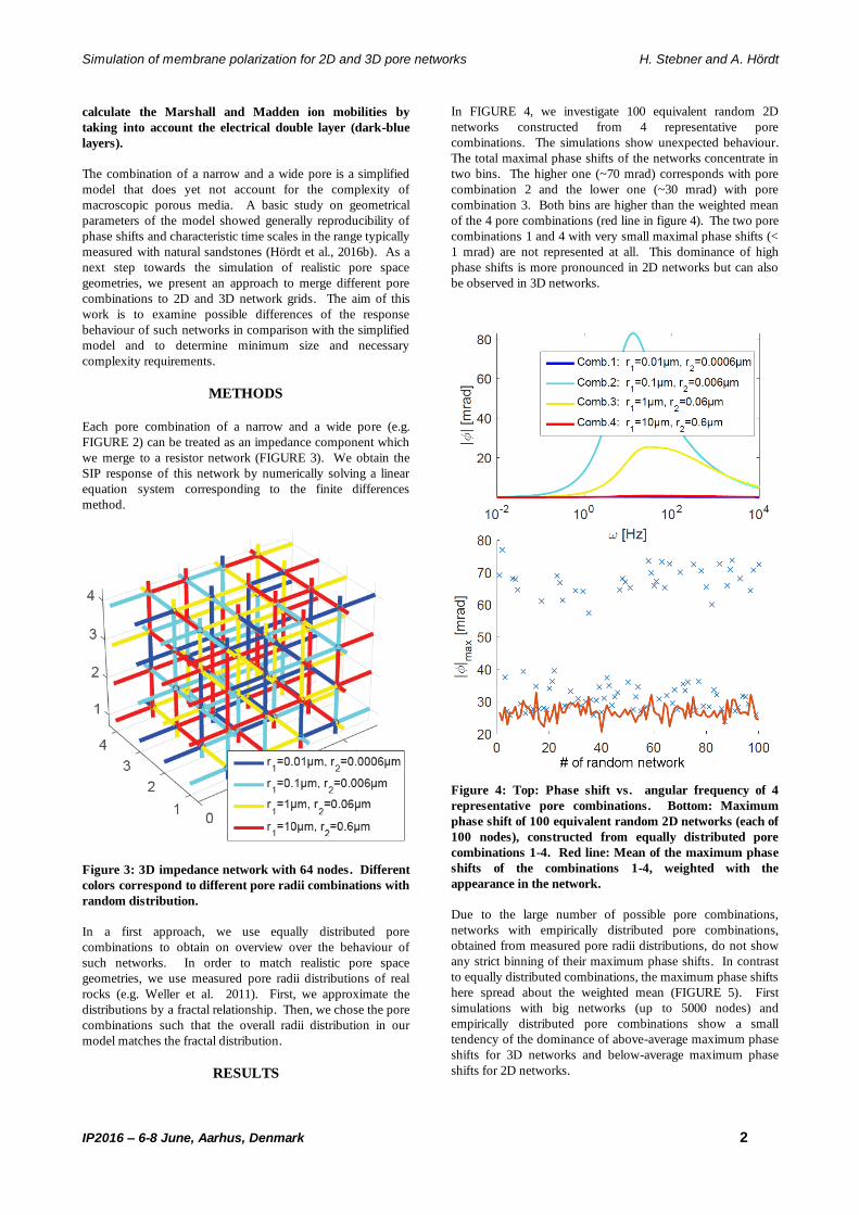
Simulation of membrane polarization for 2D and 3D pore networks H. Stebner and A. Hördt
IP2016 – 6-8 June, Aarhus, Denmark 2
calculate the Marshall and Madden ion mobilities by
taking into account the electrical double layer (dark-blue
layers).
The combination of a narrow and a wide pore is a simplified
model that does yet not account for the complexity of
macroscopic porous media. A basic study on geometrical
parameters of the model showed generally reproducibility of
phase shifts and characteristic time scales in the range typically
measured with natural sandstones (Hördt et al., 2016b). As a
next step towards the simulation of realistic pore space
geometries, we present an approach to merge different pore
combinations to 2D and 3D network grids. The aim of this
work is to examine possible differences of the response
behaviour of such networks in comparison with the simplified
model and to determine minimum size and necessary
complexity requirements.
METHODS
Each pore combination of a narrow and a wide pore (e.g.
FIGURE 2) can be treated as an impedance component which
we merge to a resistor network (FIGURE 3). We obtain the
SIP response of this network by numerically solving a linear
equation system corresponding to the finite differences
method.
Figure 3: 3D impedance network with 64 nodes. Different
colors correspond to different pore radii combinations with
random distribution.
In a first approach, we use equally distributed pore
combinations to obtain on overview over the behaviour of
such networks. In order to match realistic pore space
geometries, we use measured pore radii distributions of real
rocks (e.g. Weller et al. 2011). First, we approximate the
distributions by a fractal relationship. Then, we chose the pore
combinations such that the overall radii distribution in our
model matches the fractal distribution.
RESULTS
In FIGURE 4, we investigate 100 equivalent random 2D
networks constructed from 4 representative pore
combinations. The simulations show unexpected behaviour.
The total maximal phase shifts of the networks concentrate in
two bins. The higher one (~70 mrad) corresponds with pore
combination 2 and the lower one (~30 mrad) with pore
combination 3. Both bins are higher than the weighted mean
of the 4 pore combinations (red line in figure 4). The two pore
combinations 1 and 4 with very small maximal phase shifts (<
1 mrad) are not represented at all. This dominance of high
phase shifts is more pronounced in 2D networks but can also
be observed in 3D networks.
Figure 4: Top: Phase shift vs. angular frequency of 4
representative pore combinations. Bottom: Maximum
phase shift of 100 equivalent random 2D networks (each of
100 nodes), constructed from equally distributed pore
combinations 1-4. Red line: Mean of the maximum phase
shifts of the combinations 1-4, weighted with the
appearance in the network.
Due to the large number of possible pore combinations,
networks with empirically distributed pore combinations,
obtained from measured pore radii distributions, do not show
any strict binning of their maximum phase shifts. In contrast
to equally distributed combinations, the maximum phase shifts
here spread about the weighted mean (FIGURE 5). First
simulations with big networks (up to 5000 nodes) and
empirically distributed pore combinations show a small
tendency of the dominance of above-average maximum phase
shifts for 3D networks and below-average maximum phase
shifts for 2D networks.

Simulation of membrane polarization for 2D and 3D pore networks H. Stebner and A. Hördt
IP2016 – 6-8 June, Aarhus, Denmark 3
Figure 5: Maximum phase shift of 100 equivalent random
3D networks (each of 125 nodes), constructed from
empirically distributed pore combinations. Red line: Mean
of the maximum phase shifts of the empirical
combinations, weighted with the appearance in the
network.
CONCLUSIONS
In order to get closer to a realistic description of real rocks we
extended an existing membrane polarization model to
impedance networks. We investigated the behaviour of 3D
and 2D networks of different size and different pore
combination distributions. The choice of the distribution
function influences the SIP response behaviour. While equally
distributed pore combinations in small networks (~100 nodes)
show dominance of high phase shifts, this behaviour cannot be
confirmed with empirically distributed combinations. In big
networks (> 1000 nodes) the behaviour tends to split between
the dominance of high phase shifts for 3D and low phase shifts
for 2D networks.
Our results show that for impedance networks, higher
maximum phase shifts than the mean are in general possible.
This is more pronounced with equally distributed
combinations, but can also be shown, although with much
smaller evidence, for big 3D networks with empirically
distributed combinations. Big empirically distributed networks
are most comparable to real rocks, which allows us to get
closer to realistic SIP response modelling than with the
simplified 2-pore model only.
ACKNOWLEDGMENTS
We thank Klaus Spitzer, Ralph-Uwe Börner, Jana Börner, Julia
Weißflog and Wenke Wilhelms from Institute of Geophysics
and Geoinformatics, TU Freiberg, for useful discussions on the
numerical implementation.
The work is sponsored by the German Science foundation
(Project Ho1506/23-1).
REFERENCES
Bairlein, K., Bücker, M., Hördt, A., Hinze, B., and Nordsiek, S.
(2016). Temperature dependence of spectral induced
polarization data: experimental data and membrane
polarization theory. Geophysical Journal International.
Accepted.
Binley, A., Slater, L. D., Fukes, M., and Cassiani, G. (2005).
Relationship between spectral induced polarization and
hydraulic properties of saturated and unsaturated sandstone.
Water Resources Research, 41(W12417).
Bücker, M. and Hördt, A. (2013). Analytical modelling of
membrane polarization with explicit parametrization of pore
radii and the electrical double layer. Geophysical Journal
International., 194:804–813.
Hördt, A., Bairlein, K., Bielefeld, A., Bücker, M., Kuhn, E.,
Nordsiek, S., and Stebner, H. (2016a). The dependence of
induced polarization on fluid salinity and ph, studied with an
extended model of membrane polarization. Journal of Applied
Geophysics, accepted.
Hördt, A., Bairlein, K., and Stebner, H. (2016b). Constraints on
pore space geometries with membrane polarization, this issue.
Leroy, P., Revil, A., Kemna, A., Cosenza, P., and Ghorbani, A.
(2008). Complex conductivity of water-saturated packs of
glass beads. Journal of Colloid and Interface Science, 321:103–
117.
Marshall, D. J. and Madden, T. R. (1959). Induced
polarization, a study of its causes. Society of Exploration
Geophysicists, 24(4):790–816.
Revil, A. and Florsch, N. (2010). Determination of
permeability from spectral induced polarization in granular
media. Geophysical Journal International, 181:1480–1498.
Schwarz, G. (1962). A theory of the low-frequency dielectric
dispersion of colloidal particles in electrolyte solution. The
Journal of Physical Chemistry, 66:2636–2642.
Titov, K., Tarasov, A., Ilyin, Y., Seleznev, N., and Boyd, A.
(2010). Relationships between induced polarization relaxation
time and hydraulic properties of sandstone. Geophysical
Journal International, 180:1095–1106.
Weller, A., Breede, K., Slater, L., and Nordsiek, S. (2011).
Effect of changing water salinity on complex conductivity
spectra of sandstones. Geophysics, 76(5):F315–F327.
Weller, A., Slater, L., Nordsiek, S., and Ntarlagiannis, D.
(2010). On the estimation of specific surface per unit pore
volume from induced polarization a robust empirical relation
fits multiple data sets. Geophysics, 75(4):WA105–WA112.

IP2016 – 6-8 June, Aarhus, Denmark 1
Lithological characterization of a contaminated site using Direct current resistivity and time domain Induced Polarization
INTRODUCTION
Groundwater and surface water can be contaminated due to
various types of human activities e.g. waste from residential,
commercial, industrial, and agricultural activities. Especially
in cities with an industrial history this is often a severe
problem. In order to evaluate the risks, characterization of the
contaminated sites in terms of geology and contaminant
leachate is needed. This characterization is often carried out
using limited drill hole information, but a much more detailed
picture of the subsurface can be obtained by dense surface-
based geophysical methods.
Multi-electrode direct current (DC) resistivity and induced
polarization(DCIP) methods have proven their capability to
delineate the contaminant mass from the host geology, as
contamination strongly influences the resistivity and
chargeability of the subsurface (Gazoty et al., 2012). The
method has recently advanced in terms of data acquisition
techniques (Dahlin et. at., 2002) and processing and inversion
optimizations (Auken et al., 2009).
In this study we investigated a contaminated site using DCIP
measurements along a stream in the city of Grindsted
(southern part of Denmark) where a pharmaceutical industry
deposited massive amounts of chemicals on a number of sites.
METHODS AND RESULTS
DCIP Methodology
Direct current resistivity and Induced polarization methods
(DCIP) have been extensively used in environmental studies.
The resistivity method is based on the fact that distribution of
electrical potential in the subsurface depends on the
resistivities around a current injecting electrode. In normal
practice two electrodes are used for injection and another pair
of electrodes measures the potential. The IP method is based
on the chargeability effects of the subsurface. When
measuring in the time-domain and when the subsurface is
chargeable, the voltage does not drop immediately to zero
following the current shut down, but rather it decays slowly
over a few seconds. The magnitude of the polarization and the
shape and length of the decay depend on subsurface
parameters such as ion content and type, clay content, and
pore structure to mention a few. Time-domain IP data are
recorded along with the traditional DC data using the same
measurement setup.
Recent developments in the field of data acquisition such as
multichannel measurements (Dahlin et al., 2002) have made
the time-domain DCIP method more robust, faster and more
convenient to perform in the field. Combined with
advancements in the numerical modelling of IP data including
modelling of transmitter waveform and low-pass filters enable
us to retrieve the Cole-Cole parameters from time-domain
measurements of the entire decaying IP signal (Fiandaca et al.,
2012). The cole–cole model (Pelton et al., 1978) is a
commonly used empirical model which involves the
parameters resistivity, chargeability, relaxation time, and
frequency exponent.
Field Site and Geological Settings
The investigated study area is located in the region of southern
Denmark, Grindsted. Two of Denmark’s 122 locations
classified as "large contaminated sites" are located here
(Grindsted factory and Grindsted landfill). Contamination
from the landfill and factory site is posing great risks to
Grindsted stream and a large impact from contaminations have
been observed in the stream (Nielsen et al., 2014).
The geology of the Grindsted area consists of an upper 10-12
m quaternary sand layer and a lower tertiary sand layer,
locally separated by silt and clay layer (Heron et al., 1998).
Below this layer, we have a regional micaceous sandy layer
approximately 65 m thick, which is underlain by a clay layer
at 80 m depth.
SUMMARY Characterization tools for contaminated sites have
become advanced with the continued development of
geophysical methods. Resistivity methods and time-
domain induced polarization methods have proven their
capability to delineate the subsurface properties by
complementing each other. In the present study a large
contaminated site in Denmark was investigated using
direct current resistivity and time domain induced
polarization (DCIP). For this purpose 14 profiles were
collected alongside a stream in order to investigate the
contamination and delineate the lithological units.
2D inversion using a cole-cole model of two selected
profiles are presented. They show that the resistivity
model alone cannot depict the geology as inferred in the
borehole. However, when including the models of
chargeability and mean relaxation time the geological
units are clearly defined, which helps in identifying the
possible contaminations.
Key words: Time Domain Induced Polarization, Cole-
Cole model
Pradip Kumar Maurya Department of Geoscience
Aarhus University
C.F. Møllers Allé 4,
8000 Aarhus C
Gianluca Fiandaca Department of Geoscience
Aarhus University
C.F. Møllers Allé 4,
8000 Aarhus C
Esben Auken Department of Geoscience
Aarhus University
C.F. Møllers Allé 4,
8000 Aarhus C
Anders Vest Christiansen
Department of Geoscience
Aarhus University
C.F. Møllers Allé 4,
8000 Aarhus C
IP2016 – 6-8 June, Aarhus, Denmark 2
Data Acquisition
The site was investigated with the collection of 14 DCIP
profiles (Figure 1) covering both the north and the south bank
of the river. The profiles are will be treated in a full 3D
framework, but here we will present selected 2D results. Out
of the 14 profiles, seven profiles were 410 m long with 5 m
electrode spacing and other seven profiles were 126 m long
with 2 m electrode spacing. The survey was performed using
the gradient array (Dahlin and Zhou, 2006) and we used the
ABEM Terrameter LS for the data acquisition.
Results
The processing and inversion of the DCIP data were carried
out using Aarhus Workbench (Auken, 2009). Processing of
DCIP data involves removal of outliers from apparent
resistivity data and culling of disturbed IP decays. Data were
inverted using the 2D DCIP inversion code developed by
Fiandaca et al. (2013) .This inversion routine uses the cole-
cole model to invert the DCIP data, which gives four model
parameters namely resistivity (ρ), chargeability (m0),
relaxation time (τ) and frequency exponent (C). The inversion
code also models the full waveform and stack sizes.
Figure 2 presents the inversion results of two representative
profiles (profile 3 and 6) located at the northern bank of the
river. The cole-cole parameters shown from top to bottom are
resistivity (ρ), chargeability (m0), relaxation time (τ) and
frequency exponent (C). The borehole located on profile 6
(shown as blue dot in figure 1) is presented as a bar with the
different geological units indicated. The bar colour code
represents major lithological unit identified in borehole
(Brown: sand, light blue: sand mixed with clay, blue: clay).
It can be seen that the low resistivity anomaly in both profiles
does not clearly represent the clay rich layers seen in the
borehole. This could be attributed to the combined response of
clay layer and the contamination present in the sandy aquifer
above and below the clay layer in the north western part of the
profile.
However, in the chargeability section a high chargeability
layer agrees very well with the clay layers. This layer clearly
stands out also in the tau section. The bottom of the high
chargeable layer indicates the lower boundary of the clay
layer.
To show this boundary in the resistivity section, a red dashed
line is drawn in both profiles. We can see that in the north-
western part of both profiles the low resistivity signature is
continuing in the sandy aquifer, which possibly indicates the
presence of contaminations.
These observations indicate that the IP response is mostly
dominated by the clay rich layers, which helps in identifying
the lithological units more adequately than the resistivity
section alone.
In the presentation we will show results in 3D combining the
results of all the lines to visualize the delineation of a possible
contamination.
CONCLUSIONS DC resistivity and the time domain induced polarization
method were used at a contaminated site for characterizing the
contaminants and lithology. The results are presented in terms
of Cole-Cole parameters.
The major lithological unit could not be interpreted from the
resistivity section alone, but the chargeability section clearly
delineate the major lithological boundaries observed in a
borehole. Identification of the geological units allows for
speculations on possible contaminations identified in the
resistivity section.
ACKNOWLEDGMENTS
The authors are thankful to the Danish Council for Strategic
Research for funding the GEOCON project under which the
present study has been carried out.
REFERENCES
Auken, E., A. Viezzoli, and A. V. Christiansen, 2009, A
Single Software For Processing, Inversion, And Presentation
Of Aem Data Of Different Systems: The Aarhus Workbench,
Adelaide, ASEG.
Dahlin, T., V. Leroux, and J. Nissen, 2002, Measuring
techniques in induced polarisation imaging: Journal of
Applied Geophysics, v. 50, p. 279-298.
Dahlin, T., and B. Zhou, 2006, Multiple-gradient array
measurements for multi-channel 2D resistivity imaging: Near
Surface Geophysics, v. 4, p. 113-123.
Fiandaca, G., E. Auken, A. Gazoty, and A. V. Christiansen,
2012, Time-domain induced polarization: Full-decay forward
modeling and 1D laterally constrained inversion of Cole-Cole
parameters: Geophysics, v. 77, p. E213-E225.
Fiandaca, G., J. Ramm, A. Binley, A. Gazoty, A. V.
Christiansen, and E. Auken, 2013, Resolving spectral
information from time domain induced polarization data
through 2-D inversion: Geophysical Journal International, v.
192, p. 631-646.
Gazoty, A., G. Fiandaca, J. Pedersen, E. Auken, and A. V.
Christiansen, 2012, Mapping of landfills using time-domain
spectral induced polarization data: The Eskelund case study:
Near Surface Geophysics, v. 10, p. 575-586.
Heron, G., P. L. Bjerg, P. Gravesen, L. Ludvigsen, and T. H.
Christensen, 1998, Geology and sediment geochemistry of a
landfill leachate contaminated aquifer (Grindsted, Denmark):
Journal of Contaminant Hydrology, v. 29, p. 301-317.
Nielsen, S. S., Tuxen, N., Frimodt Pedersen, O., Bjerg, P. L.,
Sonne, A. T., Binning, P. J., Fjordbge, A. S., and Aabling, J.
(2014). Risikovurdering af over adevand, somer påvirket af
punktkildeforurenet grundvand, miljøprojekt nr 1572.
Technical report, Miljøministeriet. Miljøstyrelsen
Pelton, W. H., S. H. Ward, P. G. Hallof, W. R. Sill, and P. H.
Nelson, 1978, Mineral discrimination and removal of
inductive coupling with multifrequency IP: Geophysics, v. 43,
p. 588-609.

Figure 1 Location of DCIP profiles. Location of the borehole is shown as blue dot on profile 6.
Figure 2 DCIP inversion results from profile 3 and 6. Cole -Cole parameter shown from top to bottom are resistivity (ρ),
chargeability (m0), relaxation time (τ) and frequency exponent(C). DOI is shown by continuous black lines and dotted line in
resistivity section shows the interpreted lower boundary of the clay layer.


IP2016 – 6-8 June, Aarhus, Denmark 1
Spectral induced polarization of sand-biochar mixtures: experiments
and modeling Z. Gao Institute of Bio- and Geosciences, Agrosphere
(IBG-3), Forschungszentrum Jülich
GmbH, Germany [email protected]
F.-H. Haegel Institute of Bio- and Geosciences, Agrosphere
(IBG-3), Forschungszentrum Jülich
GmbH, Germany [email protected]
J.A. Huisman Institute of Bio- and Geosciences, Agrosphere
(IBG-3), Forschungszentrum Jülich
GmbH, Germany [email protected]
H. Vereecken Institute of Bio- and Geosciences, Agrosphere
(IBG-3), Forschungszentrum Jülich
GmbH, Germany [email protected]
INTRODUCTION
Biochar is the by-product of biomass pyrolysis and
gasification. It is derived from a wide variety of sources, including wood (Cheng et al., 2014), green waste (Chan et al.,
2007), poultry litter (Chan et al., 2008), agricultural residues
(Demirbas et al., 2006), and a wide range of additional sources. The application of biochar to farmland can increase
plant growth, reduce leaching of nutrients, and increase water
retention and microbial activity (Hunt et al., 2010).
Furthermore, biochar seems to be a promising option for long-term sequestration of carbon to offset CO2 emissions (Sohi et
al., 2009). Long-term effects of biochar in soil, however, are
not yet sufficiently investigated. Therefore suitable methods of
monitoring and investigating biochar in soil are still required to better evaluate the true agronomic and environmental value
of biochar as a soil amendment.
The physical and chemical properties of biochar vary largely
owing to different feedstocks and production processes. Characterizing biochar and its properties in soil media by
using traditional physico-chemical methods is therefore
difficult and time consuming. SIP is a promising method to
overcome these problems due to its real-time and non-invasive
features and the relatively large monitoring volumes or areas
in the field. However, modeling and understanding the SIP
signal related to the physical nature of the samples are still
challenging. Existing mechanistic models are mostly based on the theory of the polarization of the charges in the electrical
double layer (EDL) at the solid-liquid interface. These models,
however, cannot be directly applied to the polarization that is
observed in the presence of disseminated materials with electronic conductance (Gurin et al., 2013). Wong (1979)
developed a model that we refer to as the electrochemical SIP
model in the following. This model was originally proposed to
describe the SIP response of disseminated sulfide ores, which show similar electronic conductance as particles of biochar. In
this work, we study the spectral induced polarization of
disseminated biochar in sand media, and test the ability of the
electrochemical SIP model to describe the measured SIP data.
METHOD AND RESULTS
SIP Measurement
We used the SIP method to measure the complex electrical
conductivity σ* = σ’ + iσ” of mixtures of sand and sieved
biochar. The experimental set-up is shown in Figure 1. The
sample holder has a height of 18 cm and an inner diameter of 3 cm. Water can flow through the sample from the bottom to
the top of the sample holder. Flushing with electrolyte solution
was used to saturate the material inside the column and to
remove excess salts released from the biochar after sample preparation. Two porous bronze plates were used as current
electrodes at the top and bottom of the column to inject
current. Two metal potential electrodes were used at a distance
of 6 and 12 cm from the bottom of the sample holder. To avoid electrode polarization, the potential electrodes were
retracted about 1.2 cm (2 times of the diameter of the potential
electrodes) into their borings.
Figure 1. Sketch of the experimental set-up. A water tank
is connected with the bottom of the column for flushing the
sample.
SUMMARY
Biochar attracts increasing research interest due to its
potential for agricultural and environmental purposes such as soil amendment and greenhouse gas reduction.
To better monitor and investigate biochar in soil, non-
invasive measurement approaches that can be applied in
the laboratory and at field scale are needed. The goal of this work is to examine the sensitivity of the spectral
induced polarization (SIP) method to the presence of
disseminated biochar in sand. We investigate the complex electrical conductivity of saturated mixtures of sand and
sieved biochar, and use a mechanistic SIP model that
accounts for the redox reactions at the surface of the
polarized particles to invert the measured data. The magnitude of the measured complex electrical
conductivity showed a positive correlation with the mass
fraction of biochar, while the peak frequency of the
imaginary part showed a negative correlation with the particle size of the biochar. The model provides
reasonable fitting results for low mass fraction of biochar
in the mixtures.
Key words: SIP, biochar, electrochemical model
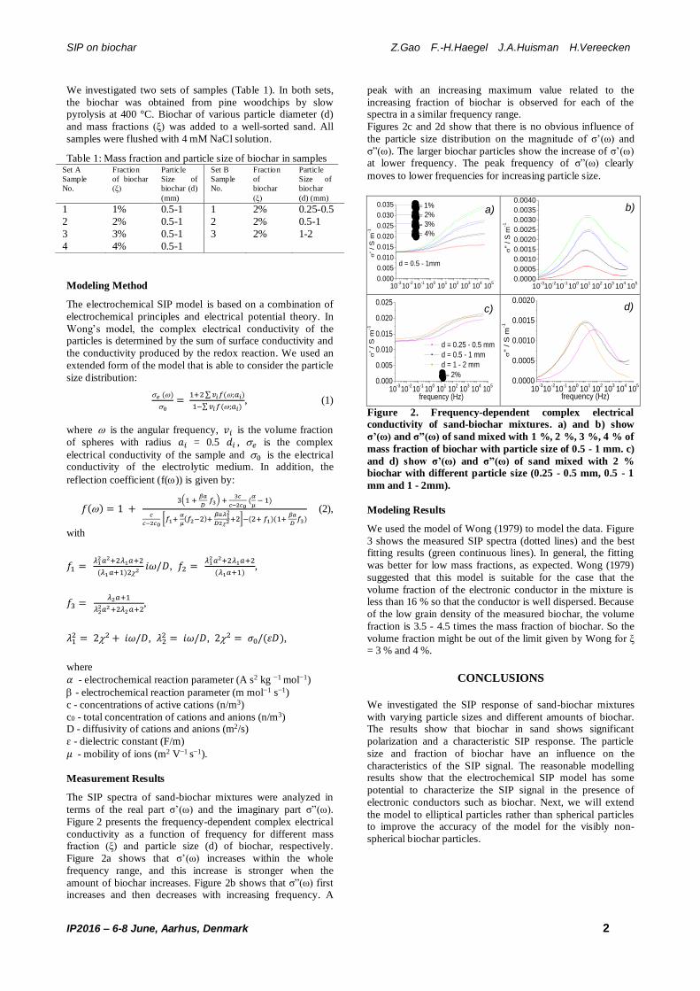
SIP on biochar Z.Gao F.-H.Haegel J.A.Huisman H.Vereecken
IP2016 – 6-8 June, Aarhus, Denmark 2
We investigated two sets of samples (Table 1). In both sets,
the biochar was obtained from pine woodchips by slow pyrolysis at 400 °C. Biochar of various particle diameter (d)
and mass fractions (ξ) was added to a well-sorted sand. All
samples were flushed with 4 mM NaCl solution.
Table 1: Mass fraction and particle size of biochar in samples Set A
Sample
No.
Fraction
of biochar
(ξ)
Particle
Size of
biochar (d)
(mm)
Set B
Sample
No.
Fraction
of
biochar
(ξ)
Particle
Size of
biochar
(d) (mm)
1 1% 0.5-1 1 2% 0.25-0.5
2 2% 0.5-1 2 2% 0.5-1
3 3% 0.5-1 3 2% 1-2
4 4% 0.5-1
Modeling Method
The electrochemical SIP model is based on a combination of
electrochemical principles and electrical potential theory. In
Wong’s model, the complex electrical conductivity of the particles is determined by the sum of surface conductivity and
the conductivity produced by the redox reaction. We used an
extended form of the model that is able to consider the particle
size distribution:
𝑒 ()
0=
1+2 ∑ 𝑣𝑖𝑓(;𝑎𝑖)
1−∑ 𝑣𝑖𝑓(;𝑎𝑖), (1)
where is the angular frequency, 𝑣𝑖 is the volume fraction
of spheres with radius 𝑎𝑖 = 0.5 𝑑𝑖 , 𝑒 is the complex
electrical conductivity of the sample and 0 is the electrical conductivity of the electrolytic medium. In addition, the
reflection coefficient (f()) is given by:
𝑓() = 1 + 3(1 +
𝛽𝑎
𝐷 𝑓3) +
3𝑐
𝑐−2𝑐0 (
𝛼
𝜇 − 1)
𝑐
𝑐−2𝑐0 [𝑓1+
𝛼
𝜇(𝑓2−2)+
𝛽𝑎𝜆12
𝐷22+2]−(2+ 𝑓1)(1+ 𝛽𝑎
𝐷𝑓3)
(2),
with
𝑓1 = 𝜆1
2𝑎2+2𝜆1𝑎+2
(𝜆1𝑎+1)22𝑖𝜔/𝐷, 𝑓2 =
𝜆12𝑎2+2𝜆1𝑎+2
(𝜆1𝑎+1),
𝑓3 = 𝜆2𝑎+1
𝜆22𝑎2+2𝜆2𝑎+2
,
𝜆12 = 22 + 𝑖𝜔/𝐷, 𝜆2
2 = 𝑖𝜔/𝐷, 22 = 𝜎0/(𝜀𝐷),
where
𝛼 - electrochemical reaction parameter (A s2 kg −1 mol−1)
- electrochemical reaction parameter (m mol−1 s−1)
c - concentrations of active cations (n/m3)
c0 - total concentration of cations and anions (n/m3) D - diffusivity of cations and anions (m2/s)
ɛ - dielectric constant (F/m)
𝜇 - mobility of ions (m2 V−1 s−1).
Measurement Results
The SIP spectra of sand-biochar mixtures were analyzed in
terms of the real part σ’(ω) and the imaginary part σ”(ω).
Figure 2 presents the frequency-dependent complex electrical
conductivity as a function of frequency for different mass fraction (ξ) and particle size (d) of biochar, respectively.
Figure 2a shows that σ’(ω) increases within the whole
frequency range, and this increase is stronger when the
amount of biochar increases. Figure 2b shows that σ”(ω) first increases and then decreases with increasing frequency. A
peak with an increasing maximum value related to the
increasing fraction of biochar is observed for each of the spectra in a similar frequency range.
Figures 2c and 2d show that there is no obvious influence of
the particle size distribution on the magnitude of σ’(ω) and
σ”(ω). The larger biochar particles show the increase of σ’(ω) at lower frequency. The peak frequency of σ”(ω) clearly
moves to lower frequencies for increasing particle size.
1%
2%
3%
4%
10-3
10-2
10-1
100
101
102
103
104
105
0.000
0.005
0.010
0.015
0.020
0.025
0.030
0.035
d = 0.5 - 1mm
' / S
m-1
10
-310
-210
-110
010
110
210
310
410
50.0000
0.0005
0.0010
0.0015
0.0020
0.0025
0.0030
0.0035
0.0040
"
/ S
m-1
10-3
10-2
10-1
100
101
102
103
104
105
0.000
0.005
0.010
0.015
0.020
0.025
d = 0.25 - 0.5 mm
d = 0.5 - 1 mm
d = 1 - 2 mm
2%' / S
m-1
frequency (Hz) 10
-310
-210
-110
010
110
210
310
410
50.0000
0.0005
0.0010
0.0015
0.0020
"
/ S
m-1
frequency (Hz)
Figure 2. Frequency-dependent complex electrical
conductivity of sand-biochar mixtures. a) and b) show
σ’(ω) and σ”(ω) of sand mixed with 1 %, 2 %, 3 %, 4 % of
mass fraction of biochar with particle size of 0.5 - 1 mm. c)
and d) show σ’(ω) and σ”(ω) of sand mixed with 2 %
biochar with different particle size (0.25 - 0.5 mm, 0.5 - 1
mm and 1 - 2mm).
Modeling Results
We used the model of Wong (1979) to model the data. Figure
3 shows the measured SIP spectra (dotted lines) and the best fitting results (green continuous lines). In general, the fitting
was better for low mass fractions, as expected. Wong (1979)
suggested that this model is suitable for the case that the
volume fraction of the electronic conductor in the mixture is less than 16 % so that the conductor is well dispersed. Because
of the low grain density of the measured biochar, the volume
fraction is 3.5 - 4.5 times the mass fraction of biochar. So the
volume fraction might be out of the limit given by Wong for ξ = 3 % and 4 %.
CONCLUSIONS
We investigated the SIP response of sand-biochar mixtures
with varying particle sizes and different amounts of biochar. The results show that biochar in sand shows significant
polarization and a characteristic SIP response. The particle
size and fraction of biochar have an influence on the
characteristics of the SIP signal. The reasonable modelling results show that the electrochemical SIP model has some
potential to characterize the SIP signal in the presence of
electronic conductors such as biochar. Next, we will extend
the model to elliptical particles rather than spherical particles to improve the accuracy of the model for the visibly non-
spherical biochar particles.
a) b)
c) d)

SIP on biochar Z.Gao F.-H.Haegel J.A.Huisman H.Vereecken
IP2016 – 6-8 June, Aarhus, Denmark 3
ACKNOWLEDGMENTS
This research was supported by the China Scholarship Council
(CSC).
REFERENCES
Chan, K. Y., Van Zwieten, L., Meszaros, I., Downie, A., and
Joseph, S., 2007, Agronomic values of greenwaste biochar as
a soil amendment: Australian Journal of Soil Research, 45, 629-634.
Chan, K. Y., Van Zwieten, L., Meszaros, I., Downie, A., and
Joseph, S., 2008, Using poultry litter biochars as soil amendments: Australian Journal of Soil Research, 46, 437-
444.
Cheng, C. H., Lin, T. P., Lehmann, J., Fang, L. J., Yang, Y. W., Menyailo, O. V., Chang, K. H., and Lai, J. S., 2014,
Sorption properties for black carbon (wood char) after long
term exposure in soils: Organic Geochemistry, 70, 53-61.
Demirbas, A., Pehlivan, E., and Altun, T., 2006, Potential
evolution of Turkish agricultural residues as bio-gas, bio-char
and bio-oil sources: International Journal of Hydrogen Energy,
31, 613-620.
Gurin, G., Tarasov, A., Ilyin, Y., and Titov, K., 2013, Time
domain spectral induced polarization of disseminated
electronic conductors: Laboratory data analysis through the Debye decomposition approach: Journal of Applied
Geophysics, 98, 44-53.
Hunt, J., DuPonte, M., Sato, D., and Kawabata, A., 2010, The basics of biochar: A natural soil amendment: Soil and Crop
Management, 30, 1-6.
Sohi, S., Lopez-Capel, E., Krull, E., and Bol, R., 2009, Biochar, climate change and soil: A review to guide future
research, CSIRO Land and Water Science Report 05/09.
Wong, J., 1979, An electrochemical model of the induced-polarization phenomenon in disseminated sulfide ores:
Geophysics, 44, 1245-1265.
Figure 3. Measured SIP spectra (dotted lines) and best fitting results for the electrochemical SIP model (green continuous
lines).
IP2016 – 6-8 June, Aarhus, Denmark 1
Numerical correction of phase errors due to leakage currents in wideband EIT measurements E. Zimmermann Central Institute for Engineering,
Electronics and Analytics,
Electronic Systems (ZEA-2) Forschungszentrum Jülich
GmbH, Germany
J. A. Huisman Institute of Bio- and
Geosciences, Agrosphere
(IBG-3),
Forschungszentrum Jülich
GmbH, Germany
A. Mester Central Institute for Engineering,
Electronics and Analytics,
Electronic Systems (ZEA-2) Forschungszentrum Jülich
GmbH, Germany
S. van Waasen Central Institute for Engineering,
Electronics and Analytics,
Electronic Systems (ZEA-2) Forschungszentrum Jülich
GmbH, Germany
INTRODUCTION
Impedance measurements on low-polarizable soils and rocks
in the mHz to kHz range require advanced data correction
methods and a sophisticated EIT measurement system to
achieve the necessary phase accuracy. For data acquisition, a
prototype spectral EIT system optimized for measurements
with high phase accuracy has been developed. In addition to
the system design, model-based numerical correction methods
are used to remove several errors introduced by amplification
errors, signal drift, current measurement errors, potential
measurement errors due to high electrode impedances, the
propagation delay of the signal due to the long cables, phase
errors introduced by inductive coupling between the electrode
cables and other system or cable dependent sources
(Zimmermann et al. 2008, Kelter et al. 2015, Zhao et al.
2015).
The use of model-based corrections enables accurate
impedance measurements for frequencies up to some kHz.
However, at test sites with high resistivity the correction
methods were not sufficient to provide accurate
measurements, which is a clear indication that an additional
phase error not yet considered in our corrections is affecting
measurement accuracy. Close inspection of the errors showed
that the remaining errors are related to capacitive leakage
currents between system ground and the soil. In this paper,
we will present a new correction method based on an
enhanced FEM model, and verify the efficiency of the new
model-based correction using impedance measurements at
resistive and conductive test sites for frequencies up to 10
kHz.
METHOD AND RESULTS
Impedance measurements were made using 30 surface
electrodes with an electrode separation of 1 m at one
conductive and one resistive field site in the vicinity of
Milano, Italy. A simple fan-shaped cable layout was used to
connect the electrodes to the measurement system. This
allows a relatively straightforward calculation of the
inductive coupling between the cables, and a subsequent
correction following the methods outlined in Zhao et al.
(2015). At the conductive test site, previously developed
model-based phase corrections worked well. However, the
corrections were not sufficient at the more resistive test site.
After analysis of the measured data, we found that there was
a strong correlation between the capacitive leakage currents
between system ground and soil and the phase response of
the measured transfer impedances. In a first attempt to
correct this error, we developed a correction method based on
a simple electrical model. However, this method did not work
well due to the inhomogeneous electrical conductivity of the
soil and the unknown and variable potential distribution at
the surface for different electrode configurations. Therefore,
it became necessary to enhance the forward FEM model to
directly consider leakage currents during the inversion of the
data. Our starting point was the following enhanced FEM
model that uses an additional admittance matrix YA to
SUMMARY
Advanced model-based data correction methods are
needed in order to determine the small phase response of
low-polarizable soils and rocks in the higher frequency
range up to 10 kHz. Methods have been developed to
correct several system-dependent errors, such as
amplification errors, signal drift, current measurement
errors, potential measurement errors due to high
electrode impedances, propagation delay of the signal
due to the long cables, and phase errors introduced by
inductive coupling between the electrode cables.
However, measurements at test sites with high resistivity
have shown a new dominating phase error, which was
found to be related to capacitive leakage currents
between system ground and the soil. In order to correct
this error, we enhanced the FEM modelling used for the
reconstruction of the electrical conductivity distribution.
Using this new formulation of the FEM forward model,
this source of error was reduced by a factor of five or
more. This enables an electrical conductivity
reconstruction for frequencies up to 10 kHz. In future
work, it will be investigated whether the capacitive
leakage currents can be reduced by optimization of the
cable layout. In any case, it is helpful to use the leakage
current as a proxy for data error during data filtering,
and it can also be used to decide if the enhanced FEM
model presented here should be used.
Key words: electrical impedance tomography, leakage
current, capacitive coupling, inductive coupling.
Abbreviated title eg: Author1, Author2 and Author3
IP2016 – 6-8 June, Aarhus, Denmark 2
consider the capacity between the cable shield and the
surface of the soil
(Y + YA) U = I (1)
where Y is the admittance matrix of the soil, U is the
potential distribution at the nodes of the used mesh, and I the
current source (Zimmerman 2011, Zhao et al. 2013). The
total capacity between system ground potential, which is also
the shield potential of the cable, and the soil is measured
with the EIT system. At the resistive test site, it was found to
be 10.5 nF. This capacity is considered in the admittance
matrix YA by assuming that the capacity is equally distributed
along all cable paths. In order to consider the effect of
leakage current, we modify the source term of the FEM
model:
I = IS + IL (2)
where the vector IS represents a symmetric current injection
(normal case) and the vector IL represents leakage currents.
Using this modified FEM model, we calculate the transfer
impedance according to:
Z = ZS + ZL (3)
where ZS is the impedance for symmetric current injection
(normal case), and the impedance ZL for excitation with the
leakage current. The leakage current is calculated from the
measured current at the two used current electrodes for all
configurations.
The modified forward FEM model is included in the
inversion in order to reconstruct the complex soil conductivity
using a 3D mesh for the forward model and a 2D mesh for
the inversion. After inversion, we calculated the corrected
impedance ZC using
ZC = ZM – ZL (4)
in order to verify the effect of the model-based correction on
the imaginary part of the measured impedance ZM.
Figure 1 shows the impedance spectra for different correction
steps. It can be seen that the correction for inductive coupling
has the biggest effect at the conductive site, whereas the
correction for capacitive leakage currents has the biggest
effect at the resistive site. After correction, the imaginary part
of the impedance is consistently negative as expected, and the
spread of the impedance values at high frequencies is
minimized. As illustrated in Figure 2, the additional model-
based correction developed in this study allows the
reconstruction of the soil conductivity for frequencies up to
10 kHz for both conductive and resistive test sites.
CONCLUSIONS
In this study, we could show that the new model-based
correction that relies on FEM modelling enables the
correction of measured impedances of resistive test sites
where leakage currents cause a strong phase error in the data.
This correction is important for wideband spectral EIT
measurements. However, it requires the measurement of the
leakage current and the total parasitic capacity between
system ground and the soil in addition to a well-defined cable
layout. Based on our current understanding, it is likely that
the cable layout can be optimized to reduce errors in
measurements of the phase of the impedance. However, the
optimal lay-out will depend on the dominating error source
(inductive coupling or capacitive leaking currents). In
addition, capacitive leaking currents increase with increasing
contact impedance of the electrodes, which thus need to be as
low as possible in order to minimize phase errors in the
impedance measurements. In any case, it is helpful to use the
leakage current as a proxy for data error during data filtering,
and it can also be used to decide if the enhanced FEM model
presented here should be used.
ACKNOWLEDGMENTS
We are grateful to Silvia Inzoli and Mauro Guidici for
support during the field measurements.
REFERENCES
M. Kelter M., Huisman, J.A., Zimmermann, E. Kemna, A.
Vereecken, H., 2015, Quantitative imaging of spectral
electrical properties of variably saturated soil columns,
Journal of Applied Geophysics, 123, 333 - 344.
Zhao, Y., Zimmermann, E., Huisman, J.A., Treichel, A.,
Wolters, B., van Waasen, S., Kemna, A., 2013. Broadband
EIT borehole measurements with high phase accuracy using
numerical corrections of electromagnetic coupling effects.
Meas. Sci. Technol. 24 (8), 085005.
Zhao, Y., Zimmermann, E., Huisman, J.A., Treichel, A.,
Wolters, B., van Waasen, S., Kemna, A., 2015. Phase
correction of electromagnetic coupling effects in cross-
borehole EIT measurements. Meas. Sci. Technol. 26 (1),
015801.
Zimmermann, E., Kemna, A., Berwix, J., Glaas, W.,
Vereecken, H., 2008. EIT measurement system with high
phase accuracy for the imaging of spectral induced
polarization properties of soils and sediments. Meas. Sci.
Technol. 19. (2008)
Zimmermann, E., 2011, Phasengenaue Impedanz-
spektroskopie und –tomographie für geophysikalische
Anwendungen (Ph.D. thesis), University of Bonn, Germany
(in German).

Figure 1. Impedance spectra of the measured and corrected transfer impedances of a more resistive (a … e) and a more
conductive (g … j) test site with the real (a, f) and imaginary part (b, g) of the uncorrected data, the imaginary part (c, h)
after correction for inductive coupling, the imaginary part after additional correction due to the capacitive leakage current
(d, i) and after additional removal of impedances with a ratio IL/IS > 10%. It should be noted that the scale can change
from step to step.
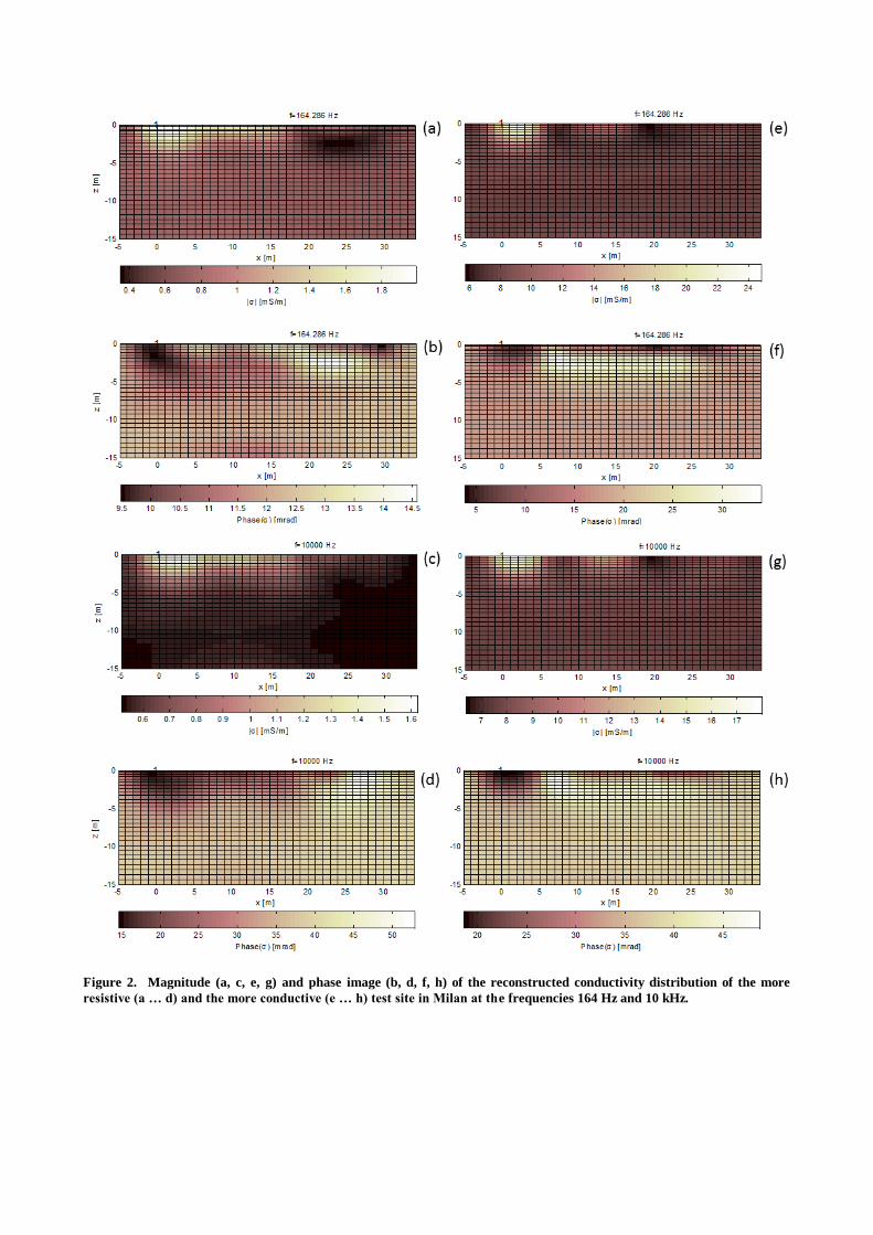
Figure 2. Magnitude (a, c, e, g) and phase image (b, d, f, h) of the reconstructed conductivity distribution of the more
resistive (a … d) and the more conductive (e … h) test site in Milan at the frequencies 164 Hz and 10 kHz.
IP2016 – 6-8 June, Aarhus, Denmark 1
Comparison of Cole-Cole and Constant Phase Angle modeling in time-domain induced polarization Myriam Lajaunie Pradip Kumar Maurya Gianluca Fiandaca
EOST HydroGeophysics Group HydroGeophysics Group, Ecole et Observatoire des Sciences de la Terre Department of Geoscience Department of Geoscience Université de Strasbourg (France) Aarhus University (Denmark) Aarhus University (Denmark) [email protected] [email protected] [email protected]
INTRODUCTION
The Induced Polarization of rocks and soils can be described
with a frequency-dependent complex resistivity. Several
models are used to describe the induced polarization of
geomaterials, but the most used are the Cole-Cole model
presented by Pelton et al. (1978) and the constant phase angle
model (CPA), as described for instance in Van Voorhis et al.
(1972).
The CPA model is suitable if no or negligible variation of the
phase shift is observed in the complex resistivity data. Thus, the
choice of using the Constant Phase Angle (CPA) model instead
of the Cole-Cole model to describe a specific set of frequency
domain IP data is straightforward. This is, however, not the case
with time domain IP data. Being able to understand how the
Cole-Cole description differs from the CPA description in time
domain will allow us to judge more easily, which description
will manage best to describe the induced polarization of a
specific studied area.
TDIP forward responses of homogeneous half-spaces have
been computed, using the Cole-Cole modeling and varying the
acquisition time ranges. Each synthetic decay has then been
inverted using the CPA modeling, in order to test to what extent
the CPA inversion is able to fit Cole-Cole data. Finally, a field
data set has been inverted using both models, to assess in a real
2D situation their ability to explain data.
METHOD AND RESULTS
The Cole-Cole and CPA models are the two principal
phenomenological models used to describe the induced
polarization of rocks and soils. The complex resistivity ζCole-Cole
of the Cole-Cole model takes the form:
𝜁𝐶𝑜𝑙𝑒−𝐶𝑜𝑙𝑒 = 𝜌(1 −𝑚0 (1 −1
1 + (𝑖𝜔𝜏)𝐶))
(1)
where ρ is the direct current resistivity, m0 is the intrinsic
chargeability, τ is the time constant, C is the frequency exponent
and i is the imaginary unit.
The CPA model is much simpler, and describes the complex
resistivity using only two parameters:
𝜁𝐶𝑃𝐴 = 𝐾(𝑖𝜔)−𝑏 (2)
where b is a positive fraction, 𝜑 = −𝜋
2𝑏 represents the phase
shift and completely defines the IP response, K is a constant and
i is the imaginary unit. In the CPA model the DC resistivity
cannot be defined, because the complex resistivity increases
indefinitely at low frequencies. For this reason Van Voorhis et
al. (1973) introduced the Drake model:
𝜁𝐷𝑟𝑎𝑘𝑒 = 𝐾(𝑖𝜔 + 𝜔𝐿)−𝑏 (3)
where in comparison with the CPA model a low frequency pole
𝜔𝐿 is introduced and the DC resistivity can be defined as 𝜌 =𝐾𝜔𝐿
−𝑏. In our implementation of the time-domain forward
response, we used the Drake model of equation (3) with a fixed
value for the low frequency pole 𝜔𝐿 = 10−5 Hz. In this way,
the inversion is set up in terms of the model parameters 𝜌 and
𝜑.
We computed synthetic time domain data using the Cole-Cole
description of the induced polarization, and tested for different
types of acquisition to what extent the CPA inversion was able
SUMMARY The Cole-Cole model and the constant phase angle (CPA)
model are two prevailing phenomenological descriptions
of the induced polarization (IP), used for both frequency
domain (FD) and time domain (TD) modeling. The former
one is a 4-parameter description, while the latest one
involves only two parameters. Choosing between a Cole-
Cole description and a CPA one to invert a specific
frequency domain data set is easy, since a look at the data
is enough to estimate their spectral content. This is,
however, not the case with TDIP data. This work aims at
understanding how the spectral content is reflected in
TDIP data, and therefore, at identifying (1) if and when it
is possible to distinguish, in time domain, between a Cole-
Cole description and a CPA one, and (2) if features of time
domain data exist in order to know, from a simple data
inspection, which model will be the most adapted to the
data. Synthetic forward responses were computed for
homogeneous Cole-Cole models, varying both time range
of the modeled IP data and Cole-Cole parameters.
Subsequently, CPA inversions were carried out on the
Cole-Cole data. The inversion results show that it is
generally possible to distinguish CPA and Cole-Cole
models in time domain, except when the Cole-Cole
frequency exponent is small (below 0.1) or for specific
combinations of the Cole-Cole parameters. The
distinctness increases with the time range of the IP data,
but usually two decades in time are sufficient to
distinguish the two models. Furthermore, forward
modeling of quadrupolar sequences on 1D and 2D
heterogeneous CPA models shows that the CPA decays
differ among each other only by a multiplication factor.
Consequently, the inspection of field data in log-log plots
gives insight on the modeling needed for fitting them: the
CPA inversion cannot reproduce the shape variability of
the IP decays. Field examples of this latter result are
presented.
Keywords: Cole-Cole, CPA, time-domain, spectral
inversion

IP2016 – 6-8 June, Aarhus, Denmark 2
to fit the synthetic data. We chose to simulate data from
homogeneous half-spaces, to be able to interpret the results of
the tests easily. The computations of forward responses and
inversions have been realized using the algorithm presented in
Fiandaca et al. (2012). We simulated different data, changing
the Cole-Cole model parameters C and τ, at fixed m0 and ρ
values. In particular, we chose as synthetic models every
possible combination of the following parameters: ρ = 100 Ωm,
m0 = 40 mV/V, C = [0.1, 0.3, 0.5], τ = [0.001, 0.01, 0.1, 1, 10]
s. Different acquisition ranges have been investigated, starting
from a reference acquisition with 40 log-increasing gates
ranging from 1 millisecond to 10 seconds. The reference
acquisition range has been reduced by (Figure 1): decreasing
the Ton=Toff values (Ton and Toff being the current on-time and
off-time, respectively), and consequently the time of the last
gate (range-type 1); increasing the delay after the current turn-
off mdly, and consequently by increasing the time of the first gate
(range-type 2);increasing mdly and decreasing Ton at the same
time (range-type 3).
Figure 1. Definition of the three acquisition range-types.
Range-type 1: the time length of the decay is increased by
adding gates at the end of the acquisition time, keeping mdly
= 1 ms (red lines). Range-type 2: the time length of the decay
is increased by adding gates at early times and keeping
Ton=Toff = 10 s (blue lines). Range-type 3: the length of the
decays is increased by adding gates both at the late and at
the early times (yellow lines).
Figure 2 shows exemplary fits of Cole-Cole decays with CPA
modeling when only 10 gates (one decade in time) are used in
the acquisition range for all the three different range-types. The
CPA inversion manages to explain the 10 gates-long curves for
any C values, and it is not possible to distinguish CPA and Cole-
Cole modeling. Figure 3 presents the CPA fits of three different
40-gates Cole-Cole decays, for different τ values (0.01 and 1
seconds) and C values (0.3 and 0.5). The shape of the Cole-Cole
forward responses changes significantly when varying τ and C,
while the shape of the CPA modeling in log-log scale remains
practically unchanged, the only difference being a translation
along the y axis. Practically, the shape of the CPA decays in
log-log scale is univocally defined by the current waveform (in
terms of current on-time Ton, current off-time Toff and stack
size). For specific combinations of τ and C parameters (e.g. τ=1
s and C=0.3) the CPA and Cole-Cole decays are really similar,
but in general the decays differ significantly.
Figure 2. CPA fits of Cole-Cole decays (5% error bars)
when varying models and range-types, but keeping constant
the number of gates (10 gates).
Figure 3. Exemplary CPA fits of Cole-Cole decays (5%
error bars, 40 gates) when varying Cole-Cole parameters.

IP2016 – 6-8 June, Aarhus, Denmark 3
Figure 4. Complete results of the synthetic tests in terms of inversion residuals (χ values, 5% error bars). The results have been
sorted according to the acquisition range-type (row), the frequency exponent (column) and the time constant (line color). For
each case, the inversion residuals are displayed as a function of the number of gates in the synthetic data.
Figure 5. Examples of field decays, along with their Cole-
Cole and CPA fits obtained through a 2D inversion.
Figure 4 shows the inversion residuals (χ values, 5% error bars)
of the CPA inversions carried out on Cole-Cole forward decays,
when varying model, range-type and number of gates. All the
models with C=0.1 present misfit below/equal to one,
regardless of the number of gates. This is easily understood
considering that the Cole-Cole model tends to the CPA model
when C goes to zero. On the other hand, with C=0.5 the two
modeling are almost always distinguishable, except for specific
models when less than two decades are used in the acquisition
time range. In particular, it is more difficult to distinguish the
CPA and Cole-Cole models for high τ values and range-type 1
when too few gates are used (i.e. when we miss the late times).
With range-type 2 the CPA and Cole-Cole models are more
difficult to distinguish with low τ values. The results with C=0.3
are similar to the results with C=0.5, except that the inversion
misfits is smaller. Interestingly, with τ=1 s the CPA and Cole-
Cole models are more difficult to differentiate, and the CPA
inversion often fits the Cole-Cole data within 5% also with 40
gates.
Finally, Figure 5 shows the comparison of CPA and Cole-Cole
modeling of field data, inverted in 2D following Fiandaca et al.
(2013). The field data were acquired at Grindsted, Denmark,
with a Terrameter LS (ABEM Instrument). We used an on-time
and an off-time of 8 s both, and 10 gates per decade (re-gating
the full-waveform data and applying the de-noising scheme
described by Olsson et. al (2016)). The data quality was
generally good, and after processing, most of the decay curves
had still ~ 30 gates. As for the synthetic modeling for
homogeneous halfspace, the shape of the CPA forward
responses does not change in log-log plots. Consequently, the
CPA description cannot explain the variety of shapes present in
the data. On the contrary, the Cole-Cole modeling is able to
retrieve the shape of the field decays.
CONCLUSIONS The synthetic results show that it is generally possible to
distinguish CPA and Cole-Cole models in time domain, except
when the Cole-Cole frequency exponent is small (below/equal
to 0.1) or for specific combinations of the Cole-Cole
parameters. The distinctness increases with the time range of
the IP data, but usually two decades in time are sufficient to
distinguish the two models. Furthermore, the shape of the CPA
forward responses in log-log plots is univocally defined by the
current waveform, also for 2D modeling. Consequently, the

IP2016 – 6-8 June, Aarhus, Denmark 4
inspection of field data in log-log plots gives insight on the
modeling needed for fitting them: the CPA inversion cannot
reproduce shape variability of the IP decays, as verified on field
examples.
ACKNOWLEDGMENTS
Support was provided by the research project GEOCON,
Advancing GEOlogical, geophysical and CONtaminant
monitoring technologies for contaminated site investigation
(contract 1305-00004B). The funding for GEOCON is provided
by The Danish Council for Strategic Research under the
Programme commision on sustainable energy and environment.
REFERENCES Cole K.S., Cole R.H., 1941. Dispersion and absorption in
dielectrics I. Alternating current characteristics. J. Chem. Phys.
9 (4), 341.
Fiandaca G., Auken E., Christiansen A.V. & Gazoty A., 2012.
Time-domain-induced polarization: Full-decay forward
modeling and 1D laterally constrained inversion of Cole-Cole
parameters, Geophysics, 77, E213-E225. 10.1190/geo2011-
0217.1.
Fiandaca G., Ramm J., Binley A., Gazoty A., Christiansen
A.V., Auken E., 2013. Resolving spectral information from
time domain induced polarization data through 2-D inversion.
Geophys. J. Int. 192 (2), 631–646.
Olsson P.I., Fiandaca G., Larsen J.J., Dahlin T., Auken E.,
2016. Doubling the spectrum of time-domain induced
polarization: removal of non-linear self-potential drift,
harmonic noise and spikes, tapered gating, and uncertainty
estimation. 4th IP Workshop, 6-8 June 2016, Aarhus, Denmark.
Pelton W.H., Ward S.H., Hallof P.G., Sill W.R., Nelson P.H.,
1978. Mineral discrimination and removal of inductive
coupling with multifrequency IP. Geophysics 43 (3), 588–609.
Van Voorhis G.D., Nelson P.H., Drake T.L., 1973. Complex
resistivity spectra of porphyry copper mineralization.
Geophysics 38 (1), 49–60

IP2016 – 6-8 June, Aarhus, Denmark 1
Airborne IP for Kimberlite Exploration
Douglas W. Oldenburg Seogi Kang University of British Columbia University of British Columbia
6339 Stores Rd., Vancouver, Canada 6339 Stores Rd., Vancouver, Canada
[email protected] [email protected]
INTRODUCTION
Figure 1(a) shows a typical geologic model of a kimberlite
composed of three different parts: crater, diatreme, and
hypabyssal facies. Physical properties of those three facies are
shown in Figure 1(b). Kimberlite exploration has focused on
looking for high magnetic susceptibility, low density and high
conductivity (Power and Hildes, 2007). The high conductivity
is often associated with lake bottom sediments as well as the
pyroclastic units at depth. The conductivity of the kimberlites
is usually found using airborne EM (AEM) surveys, and in
particular airborne time domain EM (ATEM) systems. Often
however, negative transients observed (Jansen and Witherly,
2004) indicating there is chargeable material (Weidelt, 1982).
Ice and near surface clays are known to be chargeable (Smith
and Klein, 1996), and these materials distort the AEM signals
and impede ability to extract good information about the
conductivity. As such, the existence of chargeable materials is
usually considered to be a “problem” and it is referred to as IP
contamination. The possibility exists however, that the
chargeability is reflective of the kimberlite and it is therefore
“signal” that we want to interpret.
Figure 1. (a) General structure of kimberlite pipe. (b)
Physical properties of geological units in the kimberlite
pipe.
The Tli Kwi Cho (TKC) kimberlite complex is located
approximately 360 km northeast of Yellowknife, NWT,
Canada within the Archean Slave craton. The complex is part
of the larger Lac de Gras kimberlite field. The TKC kimberlites
are composed of two main pipes called DO-18 and DO-27, and
they are respectively located at northern and southern part of
the region as shown in Figure 2(a). There are four rock units of
importance: XVK (Xenolithic kimberlite), VK (volcaniclastic
kimberlite), HK (hypabyssal kimberlite) and PK (pyroclastic
kimberlite). DO-18 pipe is mostly XVK and DO-27 is a
combination of PK and HK. The PK unit is the sought
diamondiferous portion of the pipe. An east-west geological
section at DO-27, generated from drilling results (Harder et al.,
2006) is shown in Figure 2(b). Petrophysical data including
density, susceptibility, Koenigsberger, complex conductivity
have been measured from core samples at both pipes. Figure 3
shows the measured complex impedance from TKC core
samples corresponding to PK (green), HK (red), and XVK
(purple) units.
Figure 2. Geological background of Tli Kwi Cho (TKC)
Kimberlites. (a) Plan maps of TKC with kimberlite units:
PK, HK, VK, and XVK. (b) East-west geological section of
DO-27 pipe. The map showing PK is at a shallower depth
than the map showing HK.
The impedance plots indicate that the kimberlites are
chargeable, and analysis shows that the estimated time
constants are different; PK has a much slower decay than HK
and XVK. This raises two important questions: a) Can we
invert ATEM data for chargeability? and b) Can this provide
some meaningful information about the kimberlite?
SUMMARY
Negative transients in coincident loop airborne time
domain electro-magnetic (ATEM) data have often been
observed when exploring for kimberlite deposits. It is
usually supposed that the negative transients arise from
chargeable material such as surficial clays or ice in
permafrost. As such, this EM signal is generally regarded
as a “problem” in mineral exploration because it distorts
the EM signals from the conductive kimberlites, and if not
corrected for, results in an incorrect conductivity.
However, chargeability could be reflective of the
kimberlite, hence the induced polarization (IP) effects can
be valuable “signal”. The ATEM surveys at the Tli Kwi
Cho (TKC) kimberlite complex have been a testbed for
illustrating the existence of negative transients and we
focus on that region. The two pipes that constitute TKC
have been extensively drilled and the resultant geologic
models can be used to validate our inversion results. In
addition, the complex impedance of TKC core samples
have been measured in the laboratory and the results
showed that the kimberlites can be chargeable and that
different kimberlite units have different IP characteristics.
In this paper, we first address the important issue about
depth of resolution of buried chargeable bodies relevant
to kimberlite exploration. After showing its potential we
remove the EM effects from the IP data and invert them
to recover 3D distributions of pseudo-chargeability at
multiple time channels. The recovered pseudo-charge-
ability at different times provides meaningful information
about the diamondiferous portion of the pipe and
distinguishes it from other kimberlitic rocks.
Key words: airborne EM, Induced polarization,
Kimberlite, and 3D inversion

AIP for Kimberlite Exploration Douglas W. Oldenburg and Seogi Kang
IP2016 – 6-8 June, Aarhus, Denmark 2
A major challenge for extracting IP information from airborne
data arises from the 1/r3 decay of signal away from the source
and the fact that the top few tens meters often include
permafrost and clay (Macnae, 2015). AIP is thus often thought
of as a ‘clay mapper’. Investigation of the depth resolution on
AIP is therefore crucial. We will use the geometry of TKC
pipes to address this question and then carry through an
analysis to extract geologic information from the AIP data. To
investigate depth resolution for AIP data we generate synthetic
AIP data sets with a chargeable target at different depths and
apply a 3D IP inversion to them. To proceed, we briefly outline
essential definitions and procedures. Detailed information can
be found in Kang and Oldenburg (2016).
Figure 3. Complex impedance measured from core
samples from PK (green), HK (red), and XVK (purple)
units. Left and right panel shows real and imaginary parts
of the impedance.
COMPLEX CONDUCTIVITY
Complex conductivity in the frequency domain can be
expressed as
(1)
where is conductivity at infinite frequency, and is
angular frequency (rad/s). Different descriptive models exist
but, following Smith et al. (1988), we use the Cole-Cole model
from Pelton et al. (1978):
, (2)
where is intrinsic chargeability, is time constant, and c is
frequency dependency.
LINEAR FORM OF IP RESPONSE
An ATEM observation, dobs, includes both EM and IP effects
and can be expressed as
, (3)
where the fundamental response is , which does
not include any IP effects, and dIP is the IP response. Here F []
indicates Maxwell’s operator which takes conductivity and
computes a TEM response. The IP datum can be expressed as
, (4)
This procedure can be considered as EM-decoupling because
we are removing EM induction effects from the observations.
The IP responses can be written in a linear form:
, (5)
where G is the sensitivity function and is the pseudo-
chargeability. Note that this pseudo-chargeability is time-
dependent, but the intrinsic chargeability is not. This linear
form will be the forward function that we use to invert IP data.
DEPTH INFORMATION IN AIP
The depth resolution of AIP data is limited because of the
geometric decay of the IP signal from a chargeable target. It is
often expected that the resolution is only a few tens of meters
for a compact target at the surface and about 90 m for
chargeable layers (Macnae, 2015). We systematically treat this
issue in the context of kimberlite exploration. We consider a
circular-shaped chargeable target, which is moderately
conductive and embedded in a resistive background. This
could correspond to a PK unit or a crater facies (Figure 1a).
Depth resolution of the AIP data includes two important items:
detection and delineation. For the first item, using an ATEM
survey geometry shown in Figure 1(a), we perform forward
modelling and compute dbz/dt (Figure 1b) using the EMTDIP
code (Marchant et al., 2014). The half-space earth (10-4 S/m)
includes a conductive and chargeable cylinder and Cole-Cole
parameters of the chargeable unit are =10-1 S/m, =0.1,
c=0.5 and =103 micro-s. With fixed thickness (75 m) and
radius (100 m) of the cylinder, we alter the depth from the
surface as 0, 75, and 150 m. Although the amplitude of the
observation decreases with increasing depth, the time at which
the negative value appears is almost constant (~700 micro-s)
for all three depths. Assuming a noise level of 10-3 pV/A-m2,
the detectability level is about 150 m. The cylinders at depths
of 75 or 100 meters have numerous time channels of negative
values that are well about this threshold. The main difference
of the responses at the three depths is just an amplitude factor
so it is not likely that depth information can be obtained from a
single sounding. In practice, however, we obtain ATEM data
from a number of sounding locations.
Figure 4. (a) Geometry of an ATEM system, and a
chargeable cylinder embedded in the half-space earth. (b)
Observed vertical magnetic fields (dbz/dt) with varying
depths for the chargeable unit. Solid and dotted lines
respectively indicate positive and negative data.
We perform two forward modellings: F [] (observation) and
F [ ] (fundamental) at 210 sounding locations. Then, using
Eq. (4), we evaluate the IP data at 1300 micro-s as shown in
Figure 5. As the depth increases, the IP responses get broader
and smoother due to the geometric effects. Although not
shown here, the spatial variation of the IP data hardly changes
in time, hence, this is similar to potential field data. Similar to
the inversion of magnetic data we apply a depth weighting to
compensate for the (1/r3) decay. In the following we carry out
3D IP inversions with, and without, the depth weighting
applied to IP data sets where the models had different depths
(z = 0, 75, and 150 m). Forming the sensitivity function
requires a 3D conductivity model, and we used the true
conductivity model for each case. Figure 6 shows the
recovered pseudo-chargeability models. Based upon these
results, resolving depth information looks possible and the
depth weighting seems to be advantageous, but not crucial.

AIP for Kimberlite Exploration Douglas W. Oldenburg and Seogi Kang
IP2016 – 6-8 June, Aarhus, Denmark 3
Figure 5. True IP responses computed by subtraction
using Eq. (4). Depth of the chargeable cylinder varies: a)
0m, b) 75 m, and c) 150-m depth. Dots indicate horizontal
locations of soundings.
Figure 6. Sections of recovered pseudo-chargeability at
different depths. (a) Without depth weighting and (b) with
depth weighting. Top, middle, and bottom panel corres-
pondingly indicate a chargeable target at 0, 75, and 150 m-
depth.
FIELD EXAMPLE: TKC
TKC ATEM data
Airborne EM surveys flown over TKC include DIGHEM,
AeroTEM, and VTEM systems We focus on the VTEM data
set because it illustrates the challenges we can encounter when
handling AIP data. As shown in Figure 7(a), even at the earliest
time (90 micro-s), VTEM data have negative values (dotted
contours) over DO-18 and between DO-18 and DO-27. DO-27
shows a positive anomaly (solid contour) at this time, but data
become negative at 680 micro-s as shown in Figure 7b. Easting
profile lines over DO-18 and DO-27, respectively shown in
Figure 7(c) and (d), show the transition.
Figure 7. TKC VTEM data. Maps of VTEM responses at
(a) 90 micro-s and (b) 680 micro-s. Easting profile line data
near (c) DO-18 and (d) DO-27.
3D ATEM and IP inversions
Our approach to invert AIP data is based upon Kang and
Oldenburg (2016). The first step is to invert ATEM data to
recover the conductivity. To exclude IP effects in the
observations, we only use the first 6 time channels of the
VTEM data (90-190 micro-s) near DO-27. This cannot be done
for VTEM data near DO-18 since even the earliest channel is
negative. Fortunately, DIGHEM data covers the entire TKC
area and we assume it is not significantly affected by IP, so we
cooperatively invert VTEM and DIGHEM data. The recovered
3D conductivity model is shown in Figure 8. At B-B’ section,
we overlay the boundaries of different kimberlite units
obtained from drilling results (Figure 2b). The two conductive
pipes are imaged at depth. The pipe for DO-27 extends deeper
depth than one for DO-18. The location of recovered
conductive pipe at DO-27 matches well with the PK unit.
Figure 8. Recovered 3D conductivity model. Left panel
shows plan view at 65.5 mbsf. Middle and right panels
show section views at Northing 713445m and 7133595m.
Based upon the recovered conductivity, est, we proceed with
EM-decoupling:
, (6)
where is raw IP data, F [est] is estimated fundamental
data. Figure 9 shows the observed, estimated fundamental
response, and raw IP data at 130 and 410 micro-s where both
EM and IP effects are substantial. Our EM-decoupling
effectively removes EM induction effects due to the
conductive pipe at DO-27 at both of the times evaluated here.

AIP for Kimberlite Exploration Douglas W. Oldenburg and Seogi Kang
IP2016 – 6-8 June, Aarhus, Denmark 4
dobs dI Pr aw
130micro-s
410micro-s
F [σest ]
Figure 9. Plan maps of observed (left panel), estimated
fundamental (middle panel) and raw IP (right panel) data
at 130 (top panel) and 410 (bottom panel) micro-s.
We separately invert each time channel of raw IP data and
recover 3D pseudo-chargeability at multiple times. Figure 10.
shows recovered pseudo-chargeability at 130 and 410 micro-s.
Four chargeable anomalies, A1-A4, are imaged. A1-A3 are
imaged at 130 micro-s, whereas A4 is not imaged at that time
but is apparent at 410 micro-s. This reflects the different time
decays associated with the AIP signals, and it is consistent
with the complex impedance measurements shown in Figure 3
if the A4 anomaly is a PK unit and the other anomalies, A1-A3
are associated with the other kimberlitic rocks. Through a
comparison of Figure 10 and Figure 2(a), which was obtained
from drilling, it appears that A1, A2, A3, and A4 might
respectively be connected to XVK, VK, HK, and PK units.
Recalling that PK is the most diamondiferous unit, the
recovered pseudo-chargeability at the two different times
shows that the PK unit is distinct from three other units: XVK,
VK, and HK in 3D space. In particular, at the B-B’ section
through DO-27 we have overlaid the pseudo-chargeabilty with
the geological boundaries. (see right panel of Figure 10.)
Comparisons of the boundaries and pseudo-chargeability at
130 and 410 micro-s suggests we are delineating between the
PK from HK units.
Figure 10. Recovered 3D pseudo-chargeability model at
130 (top row) and 410 (bottom row) micro-s. Left panel
shows plan view at 65.5 mbsf. Middle and right panels
show section views at Northing 713445m and 7133595m.
CONCLUSIONS
In this paper, we investigated the feasibility of the AIP
technique for kimberlite exploration and used the TKC
kimberlite region as an example. The area has been extensively
drilled and four types of kimberlitic rocks have been found.
Lab measurements on core samples showed TKC kimberlites
are chargeable and that they have different IP parameters. This
promoted two important questions: a) Can we invert ATEM
data for chargeability at depth? and b) Can the results provide
meaningful information about the kimberlite? Through the use
of a synthetic model that emulates a TKC pipe, we analyzed
the depth resolution issue and found that targets buried 75-100
meters might still be detectable and that inversion that included
a depth weighting was beneficial, but might not be crucial.
We applied a 3D ATEM-IP inversion workflow to TKC VTEM
data. To recover conductivity, we inverted early time channels
of VTEM data (presumed to have insignificant IP-
contamination) cooperatively with DIGHEM data. The details
for that result will be published in a separate paper. The
recovered conductivity includes two moderately conductive
pipes near DO-18 and DO-27. The conductivity was used to
estimate the fundamental EM response which was subtracted
from the data to generate raw IP data at multiple time
channels. 3D IP inversions were carried out and the pseudo-
chargeabilities at multiple times were obtained. Four
chargeable anomalies are imaged at depths (~70 m): A1-A4
possibly correspond to four different kimberlites: XVK, VK,
HK and PK. These correspondences can be inferred by
comparing the recovered chargeability with geologic logging in
boreholes. The recovered pseudo-chargeability at different
times suggests a distinction between the PK unit and the other
three kimberlite units. Moreover, the outline of the inferred PK
unit matches well with the boundaries of the PK unit obtained
from drilling, but some of this is likely attributed to the
conductivity model and the fact that IP sensitivities are
enhanced in regions of higher conductivity. From a geologic
perspective, the two main results might be the differentiation
of rocks associated with the two pipes. The XVK unit
comprising DO-18 is substantially different from the dominant
PK unit at DO-27. On a smaller scale, we appear to be able to
differentiate between the PK and HK units at DO-27. This is
potentially important since PK is strongly diamondiferous and
HK has minimal diamond showings. This discrimination might
be further enhanced through the use of ground IP using either
galvanic or inductive sources. Overall, our study of AIP shows
the potential benefits in kimberlite exploration, and hence
motivates further research and application in other geoscience
problems.
ACKNOWLEDGEMENTS
We thank Ken Witherly and Joel Jansen who provided the
motivation and ATEM data to carry out this research, and
Brook Clements and Jennifer Pell of Peregrine for providing
data and cores for lab measurements. We thank Dom Fournier
and Mike McMillan for their contribution to the development
of the conductivity model, and Randy Enkin of Gelogical
Survey of Cananda, Thibaut Astic, Devin Cowan and others at
UBC-GIF for participating in lab measurements and in
extensive discussions about TKC.
REFERENCES
Jansen, J., and K. Witherly, 2004, The Tli Kwi Cho kimber- lite
complex, Northwest Territories, Canada: A geophysical case
study: SEG Technical Program Expanded Abstracts, 1147–
1150.

AIP for Kimberlite Exploration Douglas W. Oldenburg and Seogi Kang
IP2016 – 6-8 June, Aarhus, Denmark 5
Kang, S., and D. W. Oldenburg, 2016, On recovering dis-
tributed IP information from inductive source time domain
electromagnetic data (in revision): Geophysical Journal In-
ternational.
Macnae, J., 2015, Quantifying Airborne Induced Polarization
effects in helicopter time domain electromagnetics: Journal of
Applied Geophysics.
Marchant, D., E. Haber, and D. Oldenburg, 2014, Three-
dimensional modeling of IP effects in time-domain elec-
tromagnetic data: Geophysics, 79, E303–E314.
Power, M., and D. Hildes, 2007, Geophysical strategies for
kimberlite exploration in northern Canada: Proceedings of
Exploration ’07: Fifth Decennial International Conference on
Mineral Exploration, 1025–1031.
Smith, R. S., and J. Klein, 1996, A special circumstance of air-
borne induced polarization measurements: Geophysics, 61,
66–73.
Smith, R. S., P. Walker, B. Polzer, and G. F. West, 1988, The
time-domain electromagnetic response of polarizable bod- ies:
an approximate convolution algorithm: Geophysical
Prospecting, 36, 772–785.
Weidelt, P., 1982, Response characteristics of coincident loop
transient electromagnetic systems: 47, 1325–1330.

IP2016 – 6-8 June, Aarhus, Denmark 1
Geometrical constraints for membrane polarization Andreas Hördt Katharina Bairlein Hermann Stebner TU Braunschweig TU Braunschweig TU Braunschweig Mendelssohnstr. 3 Mendelssohnstr. 3 Mendelssohnstr. 3 38106 Braunschweig 38106 Braunschweig 38106 Braunschweig [email protected] [email protected] [email protected]
INTRODUCTION In order to estimate hydraulic parameters of sediments from frequency-dependent electrical properties, theoretical models to simulate the electrical impedance depending on the geometrical properties of the material at the pore scale may be useful. Existing models are either based on the sedimentary grains (e.g. Leroy et al., 2008) or on the properties of the pore space (e.g. Titov et al., 2002). Here, we focus on a class of the pore-space models, describing a process called membrane polarization. Recently, Bücker and Hördt (2013a) extended the 1-D theory suggested by Marshall and Madden (1959) to two-dimensional pores. The model had some success in reproducing qualitatively some features that are commonly observed with laboratory data, such as the temperature dependence (Bairlein et al., 2016), or the increase of imaginary conductivity with increasing fluid salinity, followed by a decrease at extreme salinities (Hördt et al. 2016). So far, the model is limited to a relatively simple sequence of two types of wide and narrow cylindrical pores. In order to simulate more realistic pore geometries, one possibility is to
connect several such 2-type systems to a complex network (Stebner et al., 2016). However, since the model has many parameters and allows a huge number of parameter combinations, it is also essential to understand the model behavoir. Therefore, we review the properties of the model with a particular emphasis on the geometrical parameters, i.e. two pore lengths and pore radii. We investigate which range of parameters is necessary to obtain spectra that are typically obtained with laboratory data, and discuss whether these geometries are realistic to occur in real rocks.
THE MODEL The model suggested by Bücker and Hördt (2013a) consists of an infinite sequence of wide and narrow pores, the geometry of which is described by the pore length and pore radii (figure 1).
Figure 1. Basic model used to parameterize the pore space, consisting of a sequence of two cylindrical pore types defined by radius and length. In addition to the purely geometrical parameters, the membrane polarization depends on the ion concentration in the free fluid, ion mobility, and the properties of the electrical triple layer that builds up at the mineral surface. The triple layer is characterised by the Zeta potential and the partition coefficient that determines the distribution of the surplus charge between the Stern layer and the diffusive layer. Some of those parameters also depend on temperature and pH, as described in detail in Hördt et al. (2016). A total number of 10 parameters define the model. The basic set that is used for the study in this work, and from which variations are being carried out, is given in table 1.
SUMMARY We investigate under which conditions membrane polarization might be relevant for realistic pore space geometries. We review some basic properties of the theoretical model and illustrate general constraints by modelling studies. We focus on geometrical parameters of the model, e.g. radii r and lengths L of two cylindrical pores. In principle, a wide range of spectra can be generated, covering orders of magnitude in both maximum phase shift and characteristic time scales. One ingredient to obtain large phase shift is a small radius of the narrow pore in the range of tens of nm. Time scales are mainly controlled by pore lengths. Generating large time scales and phase shifts at the same time in principle requires large ratios between pore lengths and radii. However, within the four-dimensional parameter space, which exhibits regimes of different behaviour, examples can be found where moderate L/r ratios (10:1) can produce time scales in the range of seconds with phase shifts of a few mrad. The results encourage further attempts to combine impedances of 2-pore systems to approach the simulation of real rock systems. Key words: membrane polarization, characteristic time, phase shift, pore space.

Geometrical constraints for membrane polarization Hördt, Bairlein, Stebner
IP2016 – 6-8 June, Aarhus, Denmark 2
Property Symbol Value
Length of pore 1 L1 500 μm
Length of pore 2 L2 5 μm
Radius of pore 1 r1 200 μm
Radius of pore 2 r2 20 μm
Ion concentration c0 1 mol/m3
pH pH 6
Mobility of all ions μp1= μp2=
μn1= μn2
510-8m2/(Vs)
Zeta-potential Ϛ -75mV
Partition coefficient fQ 0,2
Temperature T 293 K
Figure 2 illustrates that a wide range of spectra may be obtained by just varying geometrical parameters. Relatively large phase shifts of several tens of mrad with the maximum at low frequencies (in this case 0,01 Hz, curve 1), corresponding to long relaxation times., intermediate phase shifts and intermediate relaxation times (curve 3), and large phase shifts combined with small relaxation times (curve 2). These curves are just a few examples, a much wider range can actually be obtained by further variations. The phase spectra in these images are relatively sharp, i.e. there is a well-defined maximum. This is a typical feature of the model, but broader spectra may of course be obtained by combining several impedances in a network.
Figure 2. Simulated phase spectra for the following parameters: 1: As given in table 1. 2: L1=5 μm, L2=0,05 μm, r1 =200nm. 3: L1=50 μm, L2=0,5 μm, r1 =1000nm. In prinicple, almost any type of reasonable spectrum might possibly be simulated theoretically. In the following, we explore the parameter space to assess which geometrical parameters required to fit data are realistic and might represent real rock conditions.
MODEL STUDIES Pore radii First, we investigate for which pore radii we obtain realistic phase shifts, typically in the range between at least 1 mrad up to several tens of mrad. Figure 3 shows the maximum phase shift, colour coded on a logarithmic scale vs. the radii of the two pores. There is a finite size zone where phase shofts are above 1 mrad. The radius of the small pore (r2) is in the tens of nm range. It is constrained by the diffusive layer thickness, defined by the Debye length (e.g. Bücker and Hördt, 2013a). If the pore is large compared to the Debye length, the relative transport of anions and cations is approximately equal, and no membrane effect exists. The radius of the second pore is roughly 10 times larger. The optimum ratio between pore radii is related to the length ratio (in this case 100:1) by a square root relationship, consistent with findings of Bücker and Hördt (2013a). The Debye length depends on several parameters, and the partition factor might also become important, such that general rules are difficult to derive. However, small pore radii in the range below 0.1 μm can be considered typical to generate measurable phase shifts.
Figure 3: Maximum phase shift extracted from the frequency-dependent spectra, colour coded vs. the radii of the two pores. The pore lengths are L1=5 μm, L2=0,05 μm, all other paramters as given in table 1. Whether or not submicron pores are relevant in real rock is not trivial to decide from independent measurements. CT images hardly have a resolution below 1 μm. Mercury injection measurements provide data down to a few nm. Weller et al. (2011) show examples of different sandstones where pore radii below 100 nm constitute more than 20% of the pore volume. Recently, Weller et al. (2015) found that they obtained better correlation between imaginary conductivity and specific internal surface area (Spor) if they use a wet-state methylene blue (MB) method instead of the conventional BET to determine Spor. The reason is that the MB method is also sensitive to the small pores in Clay minerals and thus provides higher Spor values. We take this as further evidence that pores in the range 0,1 μm and smaller, are indeed relevant in real rock.
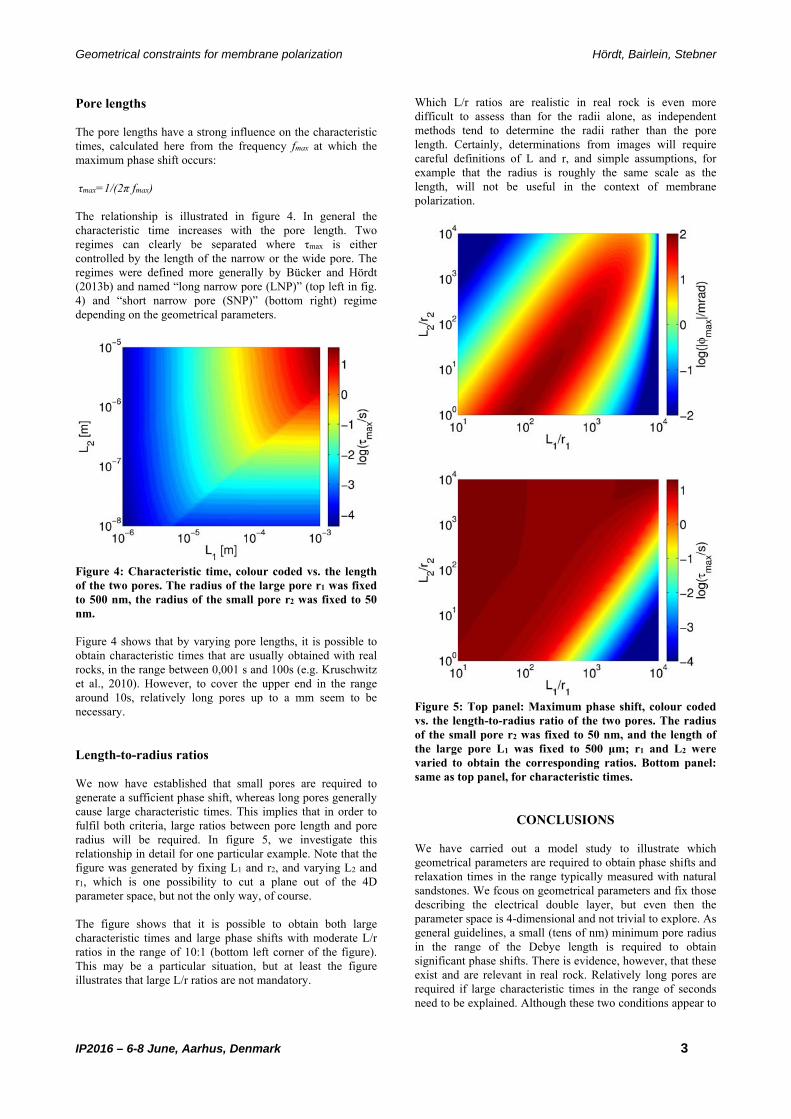
Geometrical constraints for membrane polarization Hördt, Bairlein, Stebner
IP2016 – 6-8 June, Aarhus, Denmark 3
Pore lengths The pore lengths have a strong influence on the characteristic times, calculated here from the frequency fmax at which the maximum phase shift occurs: τmax=1/(2π fmax) The relationship is illustrated in figure 4. In general the characteristic time increases with the pore length. Two regimes can clearly be separated where τmax is either controlled by the length of the narrow or the wide pore. The regimes were defined more generally by Bücker and Hördt (2013b) and named “long narrow pore (LNP)” (top left in fig. 4) and “short narrow pore (SNP)” (bottom right) regime depending on the geometrical parameters.
Figure 4: Characteristic time, colour coded vs. the length of the two pores. The radius of the large pore r1 was fixed to 500 nm, the radius of the small pore r2 was fixed to 50 nm. Figure 4 shows that by varying pore lengths, it is possible to obtain characteristic times that are usually obtained with real rocks, in the range between 0,001 s and 100s (e.g. Kruschwitz et al., 2010). However, to cover the upper end in the range around 10s, relatively long pores up to a mm seem to be necessary. Length-to-radius ratios We now have established that small pores are required to generate a sufficient phase shift, whereas long pores generally cause large characteristic times. This implies that in order to fulfil both criteria, large ratios between pore length and pore radius will be required. In figure 5, we investigate this relationship in detail for one particular example. Note that the figure was generated by fixing L1 and r2, and varying L2 and r1, which is one possibility to cut a plane out of the 4D parameter space, but not the only way, of course. The figure shows that it is possible to obtain both large characteristic times and large phase shifts with moderate L/r ratios in the range of 10:1 (bottom left corner of the figure). This may be a particular situation, but at least the figure illustrates that large L/r ratios are not mandatory.
Which L/r ratios are realistic in real rock is even more difficult to assess than for the radii alone, as independent methods tend to determine the radii rather than the pore length. Certainly, determinations from images will require careful definitions of L and r, and simple assumptions, for example that the radius is roughly the same scale as the length, will not be useful in the context of membrane polarization.
Figure 5: Top panel: Maximum phase shift, colour coded vs. the length-to-radius ratio of the two pores. The radius of the small pore r2 was fixed to 50 nm, and the length of the large pore L1 was fixed to 500 μm; r1 and L2 were varied to obtain the corresponding ratios. Bottom panel: same as top panel, for characteristic times.
CONCLUSIONS We have carried out a model study to illustrate which geometrical parameters are required to obtain phase shifts and relaxation times in the range typically measured with natural sandstones. We fcous on geometrical parameters and fix those describing the electrical double layer, but even then the parameter space is 4-dimensional and not trivial to explore. As general guidelines, a small (tens of nm) minimum pore radius in the range of the Debye length is required to obtain significant phase shifts. There is evidence, however, that these exist and are relevant in real rock. Relatively long pores are required if large characteristic times in the range of seconds need to be explained. Although these two conditions appear to

Geometrical constraints for membrane polarization Hördt, Bairlein, Stebner
IP2016 – 6-8 June, Aarhus, Denmark 4
require large L/r ratios, parameter combinations exist where moderate ratios around 10:1 are sufficient. Our results also show that speculations, membrane polarization might be particularly important at long characteristic time scales, which can sometimes be found in literature (e.g. Leroy and Revil, 2009) are not consistent with the conceptual model underlying the theory used here, as it coversa wide range of relaxation times. When attempting to match geometrical parameters typically found in real rock, it seems challenging to produce long time scales rather than short ones. The considerations here are intended to provide a general understanding of membrane polarization. Another aim is to provide guidelines for combinining impedances in networks, to get one step further towards the description of real rock geometries (Stebner et al. 2016).
ACKNOWLEDGMENTS The work is sponsored by the German Science foundation (Project Ho1506/23-1).
REFERENCES Bairlein, K., Bücker, M., Hördt, A., Hinze, B. and Nordsiek, S., 2016. Temperature dependence of spectral induced polarization data: experimental data and membrane polarization theory: Geoph. J. Int., accepted. Bücker, M., and Hördt, A., 2013a. Analytical modelling of membrane polarization with explicit parameterization of pore radii and the electrical double layer: Geoph. J. Int., doi: 10.1093/gji/ggt136.
Bücker, M., and Hördt, A., 2013b. Long and short narrow pore models for membrane polarization: Geophysics, 78, E299-E314. Kruschwitz, S., Binley, A., Lesmes, D. and Elshenawy, A. 2010. Textural controls on low-frequency electrical spectra of porous media: Geophysics 75, WA113-WA123. Leroy, P., Revil, A., Kemna, A., Cosenza, A. and Ghorbani, A. 2008. Complex conductivity of water-saturated packs of glas beads: J. of Colloid and Interface Science 321, 103-117. Leroy, P. & Revil, A. 2009. A mechanistic model for the spectral induced polarization of clay materials: J. Geoph. Res., 114, B10202. Marshall, D. J. and Madden T. R., 1959. Induced polarization: A study of its causes: Geophysics 24, 780-816. Stebner, H. and Hördt, A., 1016. Simulation of membrane polarization for 2D and 3D pore networks. this issue. Titov, K., Komarov, V. Tarasov, V. and Levitski, A. 2002. Theoretical and experimental study of time domain-induced polarization in water-saturated sands: Journal of Applied Geophysics 50, 417-433. Weller, A., Slater, L., Huismann, J.A., Esser, O., and Haegel, F.-H. 2015. On the specific polarizability of sands and sand-clay mixtures: Geophysics 76, F315-F327. Weller, A., Breede, K., Slater, L. and Nordsiek, S., 2011. Effect of changing water salinity on complex conductivity spectra of sandstones: Geophysics 76, F315-F327.