abundance trends and environmental habitat usage patterns
TRANSCRIPT
Louisiana State UniversityLSU Digital Commons
LSU Doctoral Dissertations Graduate School
2003
Abundance trends and environmental habitat usagepatterns of bottlenose dolphins (Tursiopstruncatus) in lower Barataria and Caminada Bays,LouisianaCara Edina MillerLouisiana State University and Agricultural and Mechanical College, [email protected]
Follow this and additional works at: https://digitalcommons.lsu.edu/gradschool_dissertations
Part of the Oceanography and Atmospheric Sciences and Meteorology Commons
This Dissertation is brought to you for free and open access by the Graduate School at LSU Digital Commons. It has been accepted for inclusion inLSU Doctoral Dissertations by an authorized graduate school editor of LSU Digital Commons. For more information, please [email protected].
Recommended CitationMiller, Cara Edina, "Abundance trends and environmental habitat usage patterns of bottlenose dolphins (Tursiops truncatus) in lowerBarataria and Caminada Bays, Louisiana" (2003). LSU Doctoral Dissertations. 2111.https://digitalcommons.lsu.edu/gradschool_dissertations/2111
ABUNDANCE TRENDS AND ENVIRONMENTAL HABITAT USAGE PATTERNS OF BOTTLENOSE DOLPHINS (Tursiops truncatus) IN LOWER BARATARIA AND
CAMINADA BAYS, LOUISIANA
A Dissertation
Submitted to the Graduate Faculty of the Louisiana State University and
Agricultural and Mechanical College in partial fulfillment of the
requirements for the degree of Doctor of Philosophy
in
The Department of Oceanography and Coastal Sciences
by Cara Miller
B.S., University of Portland, 1997 M.Ap.Stat., Louisiana State University, 2002
December 2003

ii
ACKNOWLEDGEMENTS
Though it’s a cliché – the journey to finally reach this point has been full of unforgettable
experiences. This dissertation is dedicated to my sister, Mum and Dad in great appreciation of
the laughter, support and love given by each of them. My sister has been always been a source
of unconditional friendship, support and kind, big-sisterly love. My Mum was willing to put her
young teenage daughter aboard a plane knowing my head was so full of dreams I would probably
not be back soon. I am very thankful that her motivated and adventurous spirit has rubbed off on
me. No one makes me laugh like my Dad - maybe I’m easily amused, but I like to think he’s
funny. Thank you Bobby Dazzler for always reminding me to “Follow my Bliss”. Additionally
I owe much to great friends like Aki, Liza, Jane, Sarah and Lesa. Lesa is one of the things I’ll
miss most about Baton Rouge. Memories of dog-paddling, sunburns, tennis and reggae music
will not be forgotten. Thanks to gentle advice from Drs. Becky Houck, Mike Bossley and Barry
Moser that provided me with small pearls of wisdom at just the right times. Some special people
were especially generous along the way including Patrick Cruise, Ray Woodforde, Shannon
Stewart and the Gordon family. I sincerely appreciate the efforts of the following volunteers
who were instrumental in my fieldwork, Lori Benson, Pat Cruise, Don Deluise, Guillermo
Duque, Donna Gavin, Rachel Gross, Heather Haas, Frank Hernandez, Holly Holwager, Annie
Leonard, Robert McGuire, Josh Molloy, Cheryl Murphy, Cat Norman, Leo Rangel, Shaye Sable
and Ted Switzer. In particular I’d like to thank my most dedicated assistant, Holly. She was
willing to skip work, classes and sleep to make fieldwork an unforgettable mix of cheese-nips,
Frank da Knife, Starfish Café dinners and continual dramas with our unreliable friend “Kitty”.
I’ve enjoyed the comradeship of lab members Ted Switzer, Guillermo Duque, Mark Stead,
Melissa Kay and Fernando Martinez. In particular Ted gave useful statistical advice, helped set-

iii
up my GIS maps, and provided some needed motivation. Last but not least I would like to thank
my committee members, Don Baltz, Barry Moser, Paul LaRock, Richard Condrey and Bill
Stickle for their role and helpful support during my graduate career. Don provided me with the
opportunity to design my own course of doctoral research and impressed upon me the
responsibility and scope that this degree required.
iv
TABLE OF CONTENTS
Page ACKNOWLEDGEMENTS …………………………………………………………………….. ii LIST OF TABLES ……………………………………………………………………………... vi LIST OF FIGURES …………………………………………………………………………... viii ABSTRACT ………………………………………………………………………………….... ix CHAPTER
I. INTRODUCTION: ASSESSING ABUNDANCE AND ENVIRONMENTAL HABITAT USAGE PATTERNS OF BOTTLENOSE DOLPHINS IN COASTAL LOUISIANA …………………………………………………………………..… 1 Literature Cited ………………………………………………………………..… 7
II. ENVIRONMENTAL HABITAT USAGE PATTERNS OF BOTTLENOSE
DOLPHINS, Tursiops truncatus, IN LOWER BARATARIA AND CAMINADA BAYS, LOUISIANA ………………………………………………………..… 10 Introduction ……………………………………………………………………. 10 Methods ………………………………………………………………………... 12 Results …………………………………………………………………………. 19 Discussion ……………………………………………………………………... 29 Conclusions ……………………………………………………………………. 38 Literature Cited ………………………………………………………………... 39
III. ASSESSMENT OF JOLLY-SEBER ASSUMPTIONS FOR NATURALLY
MARKED CETACEAN PHOTO-IDENTIFICATION DATA ……...……..… 45 Introduction ……………………………………………………………………. 45 Basic Model Assumptions …………………………………………………..… 49 Discussion ……………………………………………………………………... 53 Conclusions ……………………………………………………………….…… 65 Literature Cited ………………………………………………………………... 66
IV. MARK-RECAPTURE POPULATION ESTIMATION OF BOTTLENOSE
DOLPHINS (Tursiops truncatus) IN COASTAL LOUISIANA (1999 – 2002) ……………………………………………………..………..…. 76 Introduction …………………………………………………………………… 76 Methods ……………………………………………………………………….. 78 Results ………………………………………………………………………… 85 Discussion …………………………………………………………………….. 92 Conclusions …………………………………………………………….…….. 100 Literature Cited ……………………………………………………….……… 101

v
V. DISCUSSION ………………………………………………..………………. 106 Literature Cited ……………………………………………………………..… 109
APPENDIX: CATALOG OF INDIVIDUALS AND ADDITIONAL SIGHTING MAPS ……………………………………………………………………………………….... 113 VITA ………………………………………………………………………………………..… 125
vi
LIST OF TABLES
2.1. Seasonal frequency of groups, effort (hours), number of individuals seen and proportion of observations where feeding was observed for bottlenose dolphin groups in lower Caminada and Barataria bays, Louisiana …………………………………………………………………….... 20 2.2. Annual and seasonal patterns of environmental conditions measured in Barataria and Caminada bays, Louisiana. Significant seasonal differences (p < 0.025) were identified using least-square means (+ 1 SE) and are indicated by different letters across each row. Seasonal ranges are reported below the mean for each variable ……………………………………….... 21 2.3. Rotated factor loadings of environmental variables at bottlenose dolphins sighting locations in lower Barataria and Caminada bays, Louisiana. Magnitude and signs of factor loadings indicate strength and direction of each variable’s influence on a factor. The variance explained by each factors’s eigenvalue are expressed as absolute, proportional, and cumulative values .. 23 2.4. A forward stepwise logistic regression characterizing variables important in describing bottlenose dolphin feeding locations in lower Barataria and Caminada bays, Louisiana. Individual variables were both entered and kept in the model with a α-level of 0.20. Feeding and non-feeding least-square means ( + 1 SE) were calculated for significant continuous variables, while highest and lowest proportions of feeding activity were given for season ……………... 24 3.1. Questions arising from consideration of Jolly-Seber model assumptions in regard to cetacean photo-identification research ……………………………………………………….... 50 4.1. Ranking of the eight closed-population unequal catchability models (Otis et al. 1978) as assessed by the multivariate discriminant model selection criteria in Program CAPTURE. Rankings are based on maximum values and are presented with and without behavioral variation included in the model ………………………………………………………………………..… 90 4.2. Barataria Bay system bottlenose dolphin population size estimates (Spring 2000 – Winter 2001/02) using closed-population unequal-catchability models in Program CAPTURE …..… 91 4.3. Program MARK closed-population models with year-specific seasonal (A), yearly (B), non-year-specific seasonal (C) and constant (D) capture probabilities ranked by minimal Aikaike’s Information Criterion corrected for small sample sizes (AICc) and lowest deviance values. Likelihood ratio test (LRT) statistics were used to compare Models B, C and D with top-ranking model A and included relevant chi-square values, degrees of freedom (DF) and p-values (p) .. 93 4.4. Parameter estimates from a Program MARK closed-population model with seasonal (year-specific) probabilities of capture (Model A) where, p = sighting probability during specified time interval. The estimated population size for Model A was 176.78 (95% CL = 156.50 – 209.71) …………………………………………………………………... 93
vii
4.5. Parameter estimates from a Program MARK closed-population model with yearly probabilities of capture (Model B) where, p = sighting probability during specified time interval, and N = population size estimate. Time intervals used for 2000 and 2001 were Spring 2000 – Winter 2000/2001, and Spring 2001 – Winter 2001/2002, respectively. The estimated population size for Model B was 178.34 (95% CL = 157.59 – 211.89) ……………………..… 94 4.6. Parameter estimates from a Program MARK closed-population model with seasonal probabilities of capture (Model C) where, p = sighting probability during specified time interval, and N = population size estimate. The estimated population size for Model C was 178.21 (95% CL = 157.51 – 211.72) ……………………………………………………………………….... 94 4.7. Parameter estimates from a Program MARK closed-population model with constant probability of capture (Model D) where, p = probability of sighting throughout the study period, and N = population size estimate. The estimated population size for Model D was 179.51 (95% CL = 158.42 – 213.52) ……………………………………………………………………….... 94
viii
LIST OF FIGURES 2.1. Study site location in lower Barataria and Caminada bays, Louisiana ………………….... 13 2.2. Feeding suitability curves for temperature, dissolved oxygen, and turbidity. Vertical bars indicate frequency of overall observations (black) and feeding activity (white) for each given interval. Black lines indicate the relative suitability of variable values for feeding activity ….. 26 2.3. Feeding suitability curves for distance, depth and minimum group size. Vertical bars indicate frequency of overall observations (black) and feeding activity (white) for each given interval. Black lines indicate the relative suitability of variable values for feeding activity ….. 27 2.4. Spatial distribution of (A) minimum group size and (B) feeding and non-feeding locations of bottlenose dolphins in lower Barataria and Caminada bays, Louisiana …………………..… 28 2.5. Spatial distribution of bottlenose dolphin sightings by season in the lower Barataria bay system, Louisiana …………………………………………………………………………….... 30 2.6. Spatial distribution of minimum group sizes of bottlenose dolphin groups in Barataria and Caminada bays, Louisiana …………………………………………………………………..… 31 4.1. Study site location in lower Barataria and Caminada bays, Louisiana ………………..…. 80 4.2. Seasonal summary of bottlenose dolphin (Tursiops truncatus) group size (average minimum number of individuals per group), group sighting frequency, and hours of survey effort in Barataria and Caminada Bays, Louisiana, from June 1999 – May 2002 …………………….... 86 4.3. Number of sightings for each naturally marked dolphin that was identified in the Barataria and Caminada Bay study area from June 1999 – May 2002 ………………………………..… 87 4.4. Seasonal tabulation of the total number of naturally marked dolphins identified in the Barataria and Caminada Bay study area from June 1999 – May 2002. The number of dolphins seen only once is indicated in black, whereas the entire bar represents the total number of dolphins seen during a given season ………………………………………………………..…. 88 4.5. ‘Discovery curve’ (Williams et al. 1993) plotting the trend between newly identified naturally marked dolphins (y-axis) versus the cumulative number of dolphins observed during survey effort (x-axis) in Barataria and Caminada Bays from June 1999 – May 2002. The terminal slope (Wilson et al. 1999) was determined by looking at the slope of the last 8 (T1) and 12 (T2) % of cumulative number of individuals seen during surveys ……………………….... 89
ix
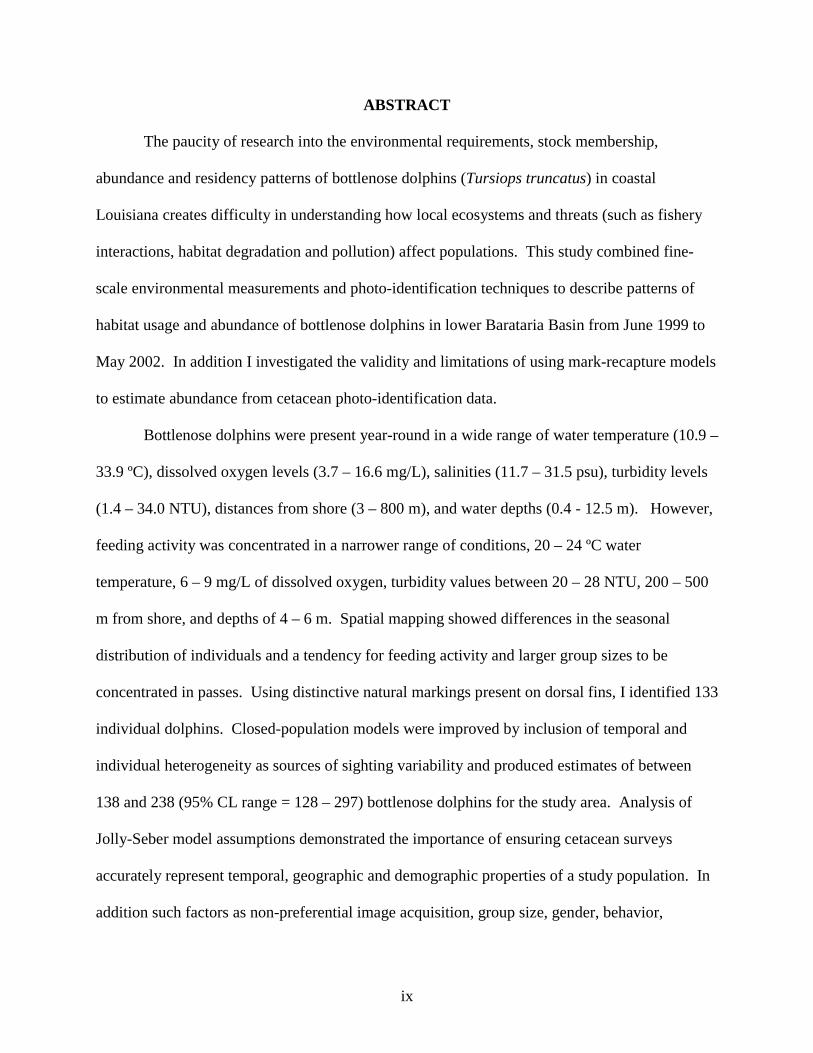
ABSTRACT
The paucity of research into the environmental requirements, stock membership,
abundance and residency patterns of bottlenose dolphins (Tursiops truncatus) in coastal
Louisiana creates difficulty in understanding how local ecosystems and threats (such as fishery
interactions, habitat degradation and pollution) affect populations. This study combined fine-
scale environmental measurements and photo-identification techniques to describe patterns of
habitat usage and abundance of bottlenose dolphins in lower Barataria Basin from June 1999 to
May 2002. In addition I investigated the validity and limitations of using mark-recapture models
to estimate abundance from cetacean photo-identification data.
Bottlenose dolphins were present year-round in a wide range of water temperature (10.9 –
33.9 ºC), dissolved oxygen levels (3.7 – 16.6 mg/L), salinities (11.7 – 31.5 psu), turbidity levels
(1.4 – 34.0 NTU), distances from shore (3 – 800 m), and water depths (0.4 - 12.5 m). However,
feeding activity was concentrated in a narrower range of conditions, 20 – 24 ºC water
temperature, 6 – 9 mg/L of dissolved oxygen, turbidity values between 20 – 28 NTU, 200 – 500
m from shore, and depths of 4 – 6 m. Spatial mapping showed differences in the seasonal
distribution of individuals and a tendency for feeding activity and larger group sizes to be
concentrated in passes. Using distinctive natural markings present on dorsal fins, I identified 133
individual dolphins. Closed-population models were improved by inclusion of temporal and
individual heterogeneity as sources of sighting variability and produced estimates of between
138 and 238 (95% CL range = 128 – 297) bottlenose dolphins for the study area. Analysis of
Jolly-Seber model assumptions demonstrated the importance of ensuring cetacean surveys
accurately represent temporal, geographic and demographic properties of a study population. In
addition such factors as non-preferential image acquisition, group size, gender, behavior,
x
stability and distinctiveness of natural markings, weather conditions and boat traffic must be
considered. Evidence of a relatively closed Barataria Basin population agrees with current
assumptions that bay bottlenose dolphin stocks are distinct from those found in deeper, offshore
waters. Furthermore, the characterization of environmental usage patterns for this bay
population strengthens adequate description and management of this relatively discrete Gulf of
Mexico bottlenose dolphin stock.
1
CHAPTER I
INTRODUCTION: ASSESSING ABUNDANCE AND ENVIRONMENTAL HABITAT USAGE PATTERNS OF BOTTLENOSE DOLPHINS IN COASTAL LOUISIANA
The Order Cetacea includes all species of whales, dolphins and porpoises. Members of
this order display a wide variety of distributional ranges, social structures, foraging styles and
life-history strategies (Reeves et al. 2002). The bottlenose dolphin (Tursiops truncatus) is one of
the most commonly studied cetacean’s worldwide (Leatherwood and Reeves 1990). Bottlenose
dolphins inhabit both coastal and offshore waters within tropical to temperate latitudes, as
evidenced by research studies conducted in such locations as Scotland (Wilson et al. 1999), the
Gulf of Mexico (Shane 1980, Wells and Scott 1990), Mexico (Ballance 1992), Portugal (Harzen
1998), Belize (Grigg and Markowitz 1997), Australia (Connor and Smolker 1985), New Zealand
(Williams et al. 1993), South Africa (Cockroft et al. 1990), and Argentina (Wursig and Wursig
1977). The variability in observed behavior and demographic parameters for these studies
indicates the flexibility and adaptability of bottlenose dolphins in different marine environments.
Individual bottlenose dolphins have relatively robust bodies with a medium sized beak and
moderately tall, falcate dorsal fins (Reeves et al. 2002). Males attain a slightly larger size than
females. Body color may be any tone of gray, with darker colors occurring dorsally while the
belly is typically off-white or pinkish in color. Calves are usually born during the warmer
months and remain associated with their mother for at least 18 months, though more commonly
about three years. Group sizes may vary anywhere from 2-15 in inshore areas, up to more than
100 individuals in offshore schools. Threats to bottlenose dolphins include sharks, habitat
degradation, fishery interactions and pollution. Depressed immune systems believed to be a
result of viral infections have been linked to major die-offs along the U.S. Atlantic and Gulf of
Mexico coasts (Reeves et al. 2002).
2
The paucity of research into bottlenose dolphin populations in coastal Louisiana creates
doubt as to present-day population size, habitat requirements, and spatial and temporal
movement patterns within the region. This dissertation focuses on characterizing abundance
trends and environmental habitat usage patterns of bottlenose dolphins in a Louisiana coastal bay
system. These objectives were achieved by conducting monthly habitat utilization and photo-
identification surveys in lower Barataria and Caminada bays (Chapter II and IV). In addition I
critically reviewed the assumptions and validity of the Jolly-Seber (J-S) model as it is commonly
used to estimate population size from cetacean photo-identification data (Chapter III).
The Gulf of Mexico covers approximately 1,500,000 km2 with an average depth of 1,700
m (Gore 1992). The principal oceanographic features for the northern Gulf of Mexico (nGOM)
region include wind stress, the Loop Current, and discharge from the Mississippi and
Atchafalaya rivers. The most distinctive circulation feature in the nGOM is the Loop Current
(Gore 1992). Warm waters from the Caribbean enter the gulf through the Yucatan Channel and
continue north along the west coast of Florida. These waters then turn clockwise and head south
until eventually exiting through the Straits of Florida. On an annual to semi-annual basis eddies
separate from the Loop Current and move west. These warm-core eddies rotate clockwise as
they transverse the Gulf waters in anywhere from a few months to a year when they reach the
shallower depths of the continental shelf and disintegrate. The Louisiana coast has undergone
significant changes in the last half century due to factors such as continued leveeing of the
Mississippi and Atchafalaya rivers, eustatic sea level rise (Day et al. 1995), canal dredging
(Turner 1997), and both natural and anthropogenic subsidence. In fact, coastal wetland losses
from 1955 to 1978 are estimated to be as high as 12,700 ha per annum (Baumann and Turner
1990). The low-lying inland wetlands include marsh grasses, submerged aquatic vegetation and
3
estuarine ponds (Chesney et al. 2000). These estuarine areas are known to provide important
habitat to juvenile fishes and crustaceans (Baltz et al. 1998) and have high primary productivity
rates (Day et al. 1989, Garrison 1999). Repercussions of wetland loss and ecosystem alterations
on coastal Louisiana marine mammal populations are unknown.
A variety of cetaceans have been observed in offshore regions of the Gulf of Mexico
(Waring et al. 2002). Whales in deep Gulf of Mexico waters (greater than 200 m) include sperm
(Physeter macrocephalus), Bryde’s (Balaenopotera edeni), Cuvier’s beaked (Ziphius
cavirostris), Blaineville’s beaked (Mesopolodon densirostris), Gervais’ beaked (Mesoplodon
europaeus), dwarf and pygmy sperm (Kogia sima and Kogia breviceps), melon-headed
(Peponocephala electra) and short-finned pilot (Globicephala macrorhynchus). Oceanic
dolphins in these same deep waters include Atlantic spotted (Stenella frontalis), bottlenose
(Tursiops truncatus), pantropical spotted (Stenella attenuata), striped (Stenella coeruleoabla),
spinner (Stenella longirostris), rough-toothed (Steno bredanensis), clymene (Stenella clymene),
frasier’s (Lagenodelphis hosei), and risso’s (Grampius griseus). Included in this same category
are the killer whale (Orcinus orca), as well as the false (Pseudorca crassidens) and pygmy
(Feresa attenuata) killer whale species.
Bottlenose and Atlantic spotted dolphins are the only cetaceans that have been reported
for inshore (depths less than 20 m) regions of the Gulf of Mexico. Inshore and offshore
bottlenose dolphin populations in the Gulf of Mexico waters are believed to be distinctive
(Waring et al. 2002). This assertion is based on the detection of hematological differences
between coastal and offshore Tursiops individuals (Duffield et al. 1983, Duffield and Wells
1986) and the assumption that movement between relatively dissimilar marine ecosystems is
limited. The 2002 U. S. Atlantic and Gulf of Mexico marine mammal stock assessments
4
(Waring et al. 2002) recognize inshore bottlenose dolphin stocks in the outer continental shelf,
coastal regions (west, north and east), as well as numerous bays, sounds and estuaries.
Population estimates are available for only three of the six inshore estuarine bottlenose dolphin
stocks in Louisiana waters (Waring et al. 2002), i.e., Bay Boudreau/Mississippi Sound region (n
= 1401), Terrebonne/Timbalier Bay complex (n = 100), and Barataria Bay (n = 219). These
estimates were based on aerial line-transect data collected in September and October of 1993
(Blaylock and Hoggard 1994). Other research into the coastal bottlenose dolphin populations of
Louisiana has been infrequent and irregular.
Habitat usage patterns (Chapter II) were examined using a fine-scale microhabitat
approach (Saucier and Baltz 1993, Baltz et al. 1998). A microhabitat is a three-dimensional
description of physical and chemical parameters at a point in space-time where a particular
organism exists. Obviously these attributes are transitory, yet compilation of a large number of
intensive microhabitat observations allows the environmental fluctuation, range and selection of
a focal species to be characterized. This approach has been used to define spawning site
selection (Saucier and Baltz 1993) as well as growth and recruitment factors (Baltz et al. 1998)
for coastal Louisiana fishes. For my study, environmental variables used to characterize patterns
of bottlenose dolphin habitat utilization were water temperature, dissolved oxygen, salinity,
turbidity, distance to shore and water depth. Additionally, temporal variables including time of
day, month, season and year were considered. Bottlenose dolphins were observed in Barataria
Basin every month throughout the duration of the study despite significant seasonal variation in
temperature, dissolved oxygen, salinity and turbidity. Variability in overall distribution of
dolphin sighting locations were examined using a principal components analysis. Patterns of
variability could be primarily attributed to season (i.e., negative correlation of temperature and
5
dissolved oxygen), space-time (evident via a positive relationship between salinity and turbidity
values) and a three-dimensional spatial component (evident with a connection between depth and
distance to shore). Important factors in feeding sites were investigated using a logistic regression
analysis. Minimum group size, temperature, turbidity and season were all determined to be
significant in describing feeding versus non-feeding locations. In a related suitability analysis,
specific ranges of all environmental variables were examined with regard to feeding. When
overall spatial distribution was examined it was apparent that areas around Caminada Pass
showed proportionately higher foraging activity. Seasonal and minimum group size distribution
patterns were not tested due to variable weather conditions.
An important approach to mark-recapture methods in wildlife research is the Jolly-Seber
open-population model (Jolly 1965, Seber 1965, Seber 1982). There have been embellishments
and additions to the original model; however, the specific ideas and concepts presented have
proven to be long lasting and valuable to the field of population estimation theory. I examined
the validity of the five Jolly-Seber assumptions with regard to cetacean photo-identification data
(Chapter III). The most obvious and recurrent factor was the premise that all samples and
surveys are a representative subset of the entire population. Additional requirements include
being aware of the temporal and geographic range of the species and adhering to randomness
stipulations. Larger scale random survey design also needs to be complemented by smaller scale
survey considerations. For example, image acquisition should be non-preferential, and factors
that may alter an individual’s probability of detection (i.e., group size, behavior or social status)
must be taken into account. Natural markings used for individual identification should be
reliable and recognizable. Finally, population parameter estimates need to be correctly
6
associated with an appropriate date or time period so that the population can be accurately
defined.
For bottlenose dolphins nicks and notches evident on the dorsal fin are suitable markings
for photo-identification (Wursig and Wursig 1977) and were used in this study of Barataria Basin
bottlenose dolphins (Chapter IV) to identify and document the behavior and movements of
individual animals. The study population appeared to be relatively closed based on a discovery
curve that approached zero (Williams et al. 1993). This curve suggested that only a few
previously unsighted marked individuals were being captured as survey effort increased.
Individual sighting histories were then used to estimate population size with Otis et al. (1978)
closed-population unequal-catchability models. The probability of sighting a given individual
varied on both a temporal scale as well as by individual. Population estimates for variously
configured models produced fairly similar population estimates (138 - 238) with an associated
95% confidence limit range of 128 - 297.
Analysis of any population needs to incorporate the specific context of the individual
under study. In marine mammal studies the context refers to the environment and ecosystem that
the individual or group inhabits (Chapter II). The limitations and requirements for any statistical
analysis need to be correctly understood to allow appropriate inferences to be made.
Examination of the Jolly-Seber model with regard to cetacean photo-identification data gave an
objective and thorough analysis of mark-recapture assumptions for a common marine mammal
research strategy (Chapter III). Analysis of individual sighting histories with respect to sources
of variability and knowledge of field methodology allowed the estimation of both defensible and
biologically realistic population estimates for bottlenose dolphins present in the Barataria Basin
(Chapter IV). Considering environmental variables that directly effect observed patterns of
7
distribution and behavior can only enhance understanding of cetacean populations. In addition,
ensuring that analyses are objective and relevant gives greater credibility and importance to
associated findings.
LITERATURE CITED Ballance, L. 1992. Habitat use patterns and ranges of the bottlenose dolphin in the Gulf of California, Mexico. Marine Mammal Science 8:262-274. Baltz, D. B., J. W. Fleeger, C. F. Rakocinski and J. N. McCall. 1998. Food, density, and microhabitat: factors affecting growth and recruitment potential of juvenile saltmarsh fishes. Environmental Biology of Fishes 53:89-103. Baumann, R. H. and R. E. Turner. 1990. Direct impact of the outer continental shelf activities on wetland loss in the central Gulf of Mexico. Environmental Geology and Water Resources 15:189-198. Blaylock, R. A. and W. Hoggard. 1994. Preliminary estimates of bottlenose dolphin abundance in southern U.S. Atlantic and Gulf of Mexico continental shelf waters. NOAA Technical Memorandum. NMFS-SEFSC-356, 10 pp. Chesney, E. J., D. M. Baltz and R. G. Thomas. 2000. Louisiana estuarine and coastal fisheries and habitats: perspectives from a fish’s eye view. Ecological Applications 10:350-366. Cockroft, V. G., G. J. B. Ross and V. M. Peddemors. 1990. Bottlenose dolphin Tursiops truncatus distribution in Natal’s coastal waters. South African Journal of Marine Science 9:1-10. Connor, R. C. and R. Smolker. 1985. Habituated dolphins (Tursiops sp.) in Western Australia. Journal of Mammalogy 66:398-400. Day, J. W. Jr., C. A. S. Hall, W. M Kemp and A. Yanez-Arancibia. 1989. Estuarine Ecology. John Wiley and Sons, New York, New York. Day, J. W. Jr., D. Pont, P. F. Hensel and C. Ibanez. 1995. Impacts of sea-level rise and on deltas in the Gulf of Mexico and the Mediterranean: the importance of pulsing events to sustainability. Estuaries 18:636-647. Duffield, D. A., S. H. Ridgway and L. H. Cornell. 1983. Hematology distinguishes coastal and offshore forms of dolphins (Tursiops). Canadian Journal of Zoology 61:930-933. Duffield, D. A. and R. S. Wells. 1986. Population structure of bottlenose dolphins: genetic studies of bottlenose dolphins along the central west coast of Florida. Contract report to
8
National Marine Fisheries Service, Southeast Fisheries Center, Contract No. 45-WCNF- 5-00366. Garrison, T. 1999. Oceanography: an introduction to Marine Science (3rd edition). Wadsworth Publishing Company, Belmont, California, U.S.A. Gore, R. H. 1992. The Gulf of Mexico: a treasury of resources in the American Mediterranean. Pineapple Press, Sarasota, FL, 384 pp. Gosselink, J. G. 2001. Comments on “Wetland loss in the northern Gulf of Mexico: multiple working hypotheses. by R. E. Turner. 1997. Estuaries 20:1-13.” Estuaries 24:636-639. Grigg, E. and H. Markowitz. 1997. Habitat use by bottlenose dolphins (Tursiops truncatus) at Turneffe Atoll, Belize. Aquatic Mammals 23:163-170. Harzen, S. 1998. Habitat use by the bottlenose dolphin (Tursiops truncatus) in the Sado estuary, Portugal. Aquatic Mammals 24:117-128. Jolly, G. M. 1965. Explicit estimates from capture-recapture data with both death and immigration – stochastic model. Biometrika 52:225-247. Leatherwood, S. and R. R. Reeves, eds. 1990. The bottlenose dolphin. Academic Press Inc., San Diego, California. Otis, D. L., K. P. Burnham, G. C. White and D. R. Anderson. 1978. Statistical inference from capture data on closed animal populations. Wildlife Monographs 62:1-135. Reeves, R. R., B. S. Stewart, P. J. Clapham and J. A. Powell. 2002. National Audobon Society guide to marine mammals of the world. Alfred A. Knopf, Inc. New York, NY. Saucier, M. and D. M. Baltz. 1993. Spawning site selection by spotted seatrout (Cynosion nebulosus) and black drum (Pogonias cromis) in Louisiana. Environmental Biology of Fishes 36:257-272. Seber, G. A. F. 1965. A note on the multiple recapture census. Biometrika 52:249-259. Seber, G. A. F. 1982. The estimation of animal abundance and related parameters (2nd edition). Griffin, London. Shane, S. 1980. Occurrence, movements, and distribution of bottlenose dolphin, Tursiops truncatus, in Southern Texas. Fishery Bulletin 78: 593-601. Turner, R. E. 1997. Wetland loss in the northern Gulf of Mexico: multiple working hypotheses. Estuaries 20:1-13.
9
Waring, G.T., J.M. Quintal and C.P. Fairfield, eds. 2002. U.S. Atlantic and Gulf of Mexico marine mammal stock assessments. NOAA Technical Memorandum NMFS-NE-169. vii + 180 + 4 app. Wells, R. S. and M. D. Scott. 1990. Estimating bottlenose dolphin population parameters from individual identification and capture-release techniques. Reports of the International Whaling Commission (Special Issue) 12:407-415. Williams, J. A., S. M. Dawson and E. Slooten. 1993. The abundance and distribution of bottlenose dolphins Tursiops truncatus in Doubtful Sound, New Zealand. Canadian Journal of Zoology 71:2080-2088. Wilson, B., P. S. Hammond and P. M. Thompson. 1999. Estimating size and assessing trends in a coastal bottlenose dolphin population. Ecological Applications 9:288-300. Wursig, B. and M. Wursig. 1977. The photographic determination of group size, composition, and stability of coastal porpoises (Tursiops truncatus). Science 198:755-756.
10
CHAPTER II
ENVIRONMENTAL HABITAT USAGE PATTERNS OF BOTTLENOSE DOLPHINS, Tursiops truncatus, IN LOWER BARATARIA AND CAMINADA BAYS, LOUISIANA
INTRODUCTION
The heterogeneous oceanic environment makes the characterization of habitat for any
marine mammal species a challenging task. Marine mammals are highly mobile, often variable
in their spatial and temporal distribution patterns, and interact with their immediate physical,
chemical and biotic environment in ways that are difficult to directly observe and quantify. It is
unclear at what resolution temporal and spatial oceanic attributes need to be examined to
determine their relationship to marine mammal distribution patterns. However, definition and
understanding of how cetaceans interact with and rely on their immediate environments allows
the possibility for insightful and informed conservation and management of individual
populations and species.
The Louisiana coastal environment has undergone significant changes in the last half
century due to factors such as continued leveeing of the Mississippi and Atchafalaya rivers,
eustatic sea level rise (Day et al. 1995), canal dredging (Turner 1997), and both natural and
anthropogenic subsidence. Coastal wetland losses from 1955 to 1978 are estimated to be as high
as 12,700 ha per annum (Baumann and Turner 1990). Estuarine areas are known to provide
important habitat to juvenile fishes and crustaceans (Baltz et al. 1998) and have high primary
productivity rates (Day et al. 1989, Garrison 1999). Repercussions of wetland loss and
ecosystem alterations on coastal Louisiana bottlenose dolphin (Tursiops truncatus) populations
are unknown. Inshore and offshore bottlenose dolphin populations in Louisiana waters are
believed to be distinctive stocks (Waring et al. 2002). This assertion is based on the detection of
hematological differences between coastal and offshore Tursiops individuals (Duffield et al.
11
1983, Duffield and Wells 1986), and the assumption that movement between relatively dissimilar
marine ecosystems is limited. Six inshore coastal bottlenose dolphin stocks are recognized in
Louisiana waters (Waring et al. 2002). However, population estimates from almost a decade ago
(Blaylock and Hoggard 1994) were reported only for the Bay Boudreau/Mississippi Sound
region (n = 1401), Terrebonne/Timbalier Bay complex (n = 100), and Barataria Bay (n = 219).
Other research into the coastal bottlenose dolphin populations in Louisiana has been infrequent
and irregular. The paucity of recent research leaves doubt as to how well these dated abundance
trends and distributional limits relate to the present day population size, habitat requirements,
and spatial and temporal movement patterns within the region.
Environmental conditions at spawning and nursery sites of coastal Louisiana fish species
have been investigated using a fine-scale microhabitat approach (Saucier and Baltz 1993, Baltz
et al. 1998). A microhabitat is a three-dimensional description of physical and chemical
conditions at an occupied site. Obviously these attributes are transitory, yet collection of a large
number of intensive microhabitat observations allows the environmental fluctuation, range and
selection of the focal species to be characterized. From this point it is possible to initiate how an
ecosystem’s qualities connect and interact with the record of activities and abundance trends of a
population.
The objective of this study was to investigate whether the distribution patterns, behavior
or observed group sizes of bottlenose dolphins present in a coastal Louisiana bay system could
be characterized by a suite of selected fine-scale environmental and temporal variables including
temperature, dissolved oxygen, salinity, turbidity, distance from shore, depth, hour of the day,
month, and year.
12
METHODS
Site Description
Barataria and Caminada bays represent the seaward interface of the Barataria Basin with
the Gulf of Mexico (Figure 2.1). Approximately 145,000 ha of salt marsh are contained within
the roughly 110 km long and 50 km wide basin (Conner and Day 1987). This relatively large
estuarine system is near to the activities of several commercially important fisheries (e.g., Gulf
menhaden purse seine, inshore shrimp trawl, and blue crab pot) and contains one of the largest
populations of bottlenose dolphins in coastal Louisiana (Waring et al. 2002). The Barataria
Basin is located along the humid, subtropical Louisiana coast directly west of the Mississippi
River (Conner and Day 1987). The climatic region is characterized by hot, humid summers with
relatively mild winters. Barataria and Caminada bays lie in the lower saline portion of the basin
and are separated from the Gulf of Mexico by a series of barrier islands (Reed 1995). The bays
average 1.6 m of precipitation per year, and salinity typically ranges between 6 and 22 practical
salinity units (psu). Bay waters are both shallow (mean depth is 1.5 m) and turbid, with the
diurnal tide range averaging around 30 cm (Connor and Day 1987). Bottom sediments are
composed primarily of silt, clay and organic detritus, but sand, shell and shell fragments are also
present. Common marsh vegetation types in this region include Spartina alterniflora (smooth
cord grass), Juncus roemerianus (black rush), Distichilis spicata (saltgrass), Batis maritima
(saltwort), and Salicornia virginica (glasswort) (Day et al. 1989).
Survey Methodology
Monthly surveys began in June 1999 and continued until May 2002. General physical
and geographical characteristics, such as connectivity to the Gulf of Mexico and proximity to
industrial areas, were used to divide the study area into six strata. Random sequence and order

13
2 0 2 4 Miles
S
N
EW
Barataria Bay
Grande Terre
Gulf of Mexico
Caminada Pass
Caminada Bay
Grande Isle
Barataria Pass
Figure 2.1. Study site location in lower Barataria and Caminada Bays, Louisiana.
14
of entrance into each of these strata created a stratified random sampling design. Two or more
independent observers used a small motorboat during each month to survey all six strata. Once
an individual or group was sighted, the boat was slowed and the individual or group was
approached. The latitude and longitude of the initial observation site was marked with a hand-
held geographic positioning system (GPS). Standard photo-identification techniques (Wursig
and Wursig 1977) were used to photograph as many dorsal fin profiles as possible to be used in a
complementary photo-identification population assessment of bottlenose dolphins in the area.
This technique allows identification of individual dolphins by documenting natural markings
present on the dorsal fin (see Chapters III and IV). After voluntary departure from the initial
observation site, the boat was moved to the site to collect microhabitat data. The ultimate
microhabitat of an individual is the site it occupies at a given point in time (Hurlbert 1981).
Direct measurements made at observation sites were conducted to describe trends in microhabitat
selection of individuals and groups of bottlenose dolphins. Environmental variables used to
characterize microhabitat were water temperature, dissolved oxygen, salinity, turbidity, distance
to shore and water depth. Additionally, temporal variables including time of day, month, season
and year were considered in this study. Sea-surface temperature (°C), salinity (psu) and
dissolved oxygen (mg/L) were measured with a Hydrolab Environmental Data Systems model
SCR2-SU Sonde unit or the combination of a YSI model 33 S-C-T meter and a YSI model 57
oxygen meter. Water depth was determined with a weighted line marked at 10 cm intervals. A
superficial substrate sample from the bay floor was obtained from a small scoop attached to a 4
m push-pole. When depths exceeded the line or push-pole length, nautical charts were
referenced for depth and substrate type. Distance from shore was estimated by measuring the
distance between the initial observation site and the nearest land point from detailed maps of the
15
area. Water samples were collected for laboratory assessment of Nephloid Turbidity Units
(NTU) using a Moniteck nephelometer or Hach 2100N Turbidimeter. Bottlenose dolphin group
size and composition was recorded, including estimates of minimum, best, and maximum group
size (Urian and Wells 1996) and the presence of juveniles and calves were noted. An individual
was identified as juvenile if it was less than 80% of adult size. Individuals identified as calves
exhibited two or more of the following, approximately 50% of adult size, dark coloration, limp
dorsal fin, calf “head-out” surfacing pattern, neonatal vertical stripes, and consistently surfacing
in “calf position” (Urian and Wells 1996). Behaviors were categorized using the following
descriptors (Urian and Wells 1996, Allen and Read 2000): (1) Foraging – Fish in mouth, rapid
and deep diving, quick circling behavior at the water surface, or direct pursuit of a prey item, (2)
Social – Play, sexual encounters, leaping, tail-chuffing, and all other general interactive
activities, (3) Rest – Slow bobbing and lack of relative motion, and (4) Travel – Directed
movement, zig-zag swimming and milling. All sightings were made during daylight hours (0750
– 1850 hrs). Sighting conditions were characterized by recording Beaufort sea state, sea state,
general weather conditions (such as sun, clouds or rain) and presence of glare. After all details
were recorded, effort was continued at or near the point on the survey line from where the
individual or group was initially sighted.
Statistical Methods
Monthly observations were pooled into seasons defined as Fall – (September, October
and November), Winter (December, January and February), Spring – (March, April and May),
and Summer – (June, July and August). Statistical analyses were conducted using SAS software
Version 8.02 (SAS Institute 1996) unless otherwise noted. Environmental variables were
assessed for univariate and bivariate normality. Power transformations were invoked to improve
16
normality where necessary (Freund and Wilson 1997). Seasonal differences between the
environmental variables, including temperature, dissolved oxygen, salinity, turbidity, distance
from shore and depth, were assessed using a multivariate analysis of variance (MANOVA).
Pairwise comparisons were performed on variables that produced a significant Shapiro-Wilks
result (p value < 0.05). Least-square means methods with Tukey’s adjustment were used to
indicate the character of significant seasonal differences. Overall and seasonal means and
standard errors of each environmental variable were also computed. To establish whether
sighting conditions differed between seasons, Beaufort Sea state values were assessed in an
identical manner to the environmental variables.
A principal components analysis (PCA) of six environmental variables (temperature,
dissolved oxygen, salinity, turbidity, distance from shore, and depth) was employed to examine
the pattern of variability in habitat use by bottlenose dolphins. Only principal components with
eigen values greater than one were chosen for further analysis as they accounted for more
variation than an original variable. Inspection of the scree plot was used to confirm that the
selected eigen values described a relatively large proportion of total data variability. To aid in
interpretation a varimax rotation was used on selected orthogonal components.
Foraging observations were compared to all other observations to determine whether
environmental conditions where feeding occurred were distinct. All behaviors associated with
foraging, including direct contact, rapid and deep diving, quick circling behavior at the water’s
surface, and direct pursuit of a prey item, were scored as feeding activity. Non-feeding
behaviors included social interactions, rest and travel. In cases where prominent behavior was
indeterminable, activity was conservatively categorized as non-feeding. A logistic regression
and habitat suitability curves (Saucier and Baltz 1993) were developed to investigate whether
17
particular environmental variables were useful in describing feeding activity. A logistic
regression uses maximum likelihood estimation to select variables that are most likely to predict
the observed results. Residuals follow a binomial distribution so neither homoscedasticity nor
normality of individual variables are required; however, multicollinearity between independent
variables should be minimal (Allison 1991) and was assessed by variance inflation factors (VIF).
Variables that are primarily independent should produce VIF values close to 1, with no
individual value greater than 10. Specific independent variables investigated were temperature,
dissolved oxygen, salinity, turbidity, distance from shore, depth, time of day, season and
minimum number of individuals present in a group. Variables included in the logistic regression
were considered one at a time using a forward stepwise approach. Entry and exit p-values of 0.2
were chosen to identify a suite of variables that may be important even if not significant. The
variable with the greatest Chi-square score (also with an associated p-value ≤ 0.2) is the one that
most reduces the log likelihood of the overall model. The next variable is chosen in the same
manner; however, after each addition all variables in the model were examined via a Wald Chi-
square test to ensure that they remained significant (i.e., Pr > Chi-square is less than or equal to
0.2). If the variable was no longer significant, it was eliminated from the model. The goodness-
of-fit of the final model was evaluated via a Hosmer and Lemeshow test (Allison 1991) in which
a non-significant Chi-square value indicates a good fit. Least-square means with associated
standard deviations of feeding and non-feeding observations were computed for all significant
variables. To describe seasonal feeding activity, seasons in which the highest proportion of
feeding and non-feeding observations took place were calculated.
Habitat suitability curves were constructed to characterize habitat selection at feeding
sites (Baltz 1990). This approach considers the proportional frequency of feeding activity across
18
individual environmental gradients in relation to the proportional availability of an
environmental variable at intervals along its observed range. Both the entire data set (i.e.,
resource availability) as well as the subset of observations where feeding occurred (i.e., resource
use) were used to construct univariate frequency distributions and suitability curves. In addition,
habitat selection for group size was assessed also. Specifically, feeding habitat suitability (S) for
each defined interval of a given variable’s range was calculated using the following formula:
S = P (E|F) / P (E)
where P(E|F) is the probability of a feeding observation, and P(E) is the total number of
observations (Baltz 1990). Habitat suitability values were normalized to a scale of 0 (non-
feeding) to 1 (high probability of feeding) by dividing through by the highest calculated raw
suitability value for the given environmental variable. In addition, each of the univariate
frequency distributions of the temporal and environmental variables was examined on an
individual basis.
A Geographic Information System (GIS) was created to visualize the spatial distribution
patterns of individual bottlenose dolphin sightings within the study area. Maps were prepared
with ArcGIS 3.2 software (Breslin et al. 1999, Longley et al. 2001, Ormsby et al. 2001). Season,
behavior and minimum group size were differentiated on projections of the study area to
examine patterns of distribution. To examine areas of proportionally higher feeding activity the
entire study area was divided into 16 equally sized quadrats for which the overall number of
observations as well as the frequency of feeding activity was tabulated. Additional analyses on
minimum group size and season were not undertaken due to variability in the ability to detect
individuals between seasons, as well as the higher probability of seeing larger group sizes.
Anomalous behavior of an oxygen probe required division of the data set. All multivariate
19
statistical methods used the subset of observations where the Hydrolab Environmental Data
Systems model SCR2-SU Sonde unit was used to measure dissolved oxygen content. This
subset constituted the first 194 observations taken (June 1999 – May 2001). Univariate analyses
on all other environmental variables used the entire dataset (n = 269).
RESULTS
On 44 survey days between June 1999 and May 2002, a total of 269 bottlenose dolphin
individuals or groups were observed in the lower reaches of Caminada and Barataria bays.
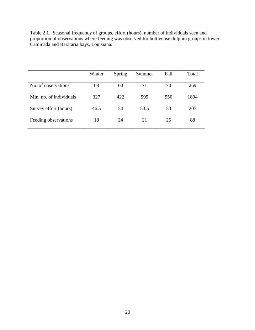
Number of groups, total number of individuals, incidence of feeding, and survey effort were
tabulated on a seasonal basis (Table 2.1). Observations and survey effort were distributed
relatively evenly across seasons. A MANOVA detected significant seasonal differences in
temperature, dissolved oxygen, salinity and turbidity. Posterior pairwise comparisons using
least-square means with a Tukey adjustment indicated seasonal differences for 4 of 6
environmental variables (Table 2.2). No seasonal differences in distance from shore or water
depth were detected so these variables were not examined further. Temperature was
significantly different between all four seasons. Lowest temperatures were measured in winter,
and then progressively increased through spring, fall and lastly summer. The lowest dissolved
oxygen levels were found at similar levels in summer and fall. Dissolved oxygen content
climbed significantly in fall and again in winter. Mean salinity values fell into two general
groupings: fall-winter salinities were higher than summer-spring. These groupings are not
readily visible because listed results do not show that the p-value for differences between spring
and fall was 0.028. Fall turbidity levels were significantly lower than winter and spring;
however, differences in turbidity were not evident between summer, spring and winter. Beaufort
sea state values were significantly different between seasons (p < 0.0002). Summer sea state was
20
Table 2.1. Seasonal frequency of groups, effort (hours), number of individuals seen and proportion of observations where feeding was observed for bottlenose dolphin groups in lower Caminada and Barataria bays, Louisiana.
Winter Spring Summer Fall Total
No. of observations 68 60 71 70 269
Min. no. of individuals 327 422 595 550 1894
Survey effort (hours) 46.5 54 53.5 53 207
Feeding observations 18 24 21 25 88

21
Table 2.2. Annual and seasonal patterns of environmental conditions measured in Barataria and Caminada bays, Louisiana. Significant seasonal differences (p < 0.025) were identified using least-square means (+ 1 SE) and are indicated by different letters across each row. Seasonal ranges are reported below the mean for each variable.
Variable Winter Spring Summer Fall Overall mean (+ 1 SE)
Temperature (°C)
13.96 + 0.45 A
(10.89 - 18.00)
23.00 + 0.47 B
(19.55 - 30.40)
30.12 + 0.44 C
(29.53 - 33.90)
25.99 + 0.44 D
(17.52 - 30.33)
23.37 + 0.43
Dissolved Oxygen (mg/L)
11.58 + 0.28 A
(8.38 - 16.63)
9.07 + 0.27 B
(4.79 - 14.55)
6.99 + 0.30 C
(3.67 - 11.10)
7.90 + 0.29 C
(5.70 - 10.55)
8.98 + 0.19
Salinity (psu)
24.15 + 0.51 A
(19.6 - 31.5)
21.99 + 0.54 B
(12.60 - 28.6)
20.84 + 0.50 B
(11.7 - 28.5)
24.06 + 0.50 A
(23.0 - 28.3)
22.77 + 0.27
Turbidity (NTU)
14.15 + 0.87 A
(4.1 - 34.0)
13.50 + 0.92 A
(1.56 - 28.1)
11.19 + 0.85 AB
(4.40 - 27)
9.76 + 0.85 B
(1.4 - 29.00)
12.08 + 0.45
Distance (m)
69.04 + 12.78
(10 - 300)
111.42 + 13.61
(5 - 500)
91.73 + 12.51
(3 - 600)
70.14 + 12.60
(10 - 800)
84.77 + 6.47
Depth (m)
2.82 + 0.23
(0.40 - 12.5)
2.54 + 0.25
(0.45 - 7.0)
2.33 + 0.23
(0.46 - 8.0)
2.72 + 0.23
(0.60 - 9.50)
2.60 + 0.12
22
found to be significantly lower than both winter and fall. In addition to summer, winter sea state
was close to being significantly greater than those observed in spring surveys (p < 0.03).
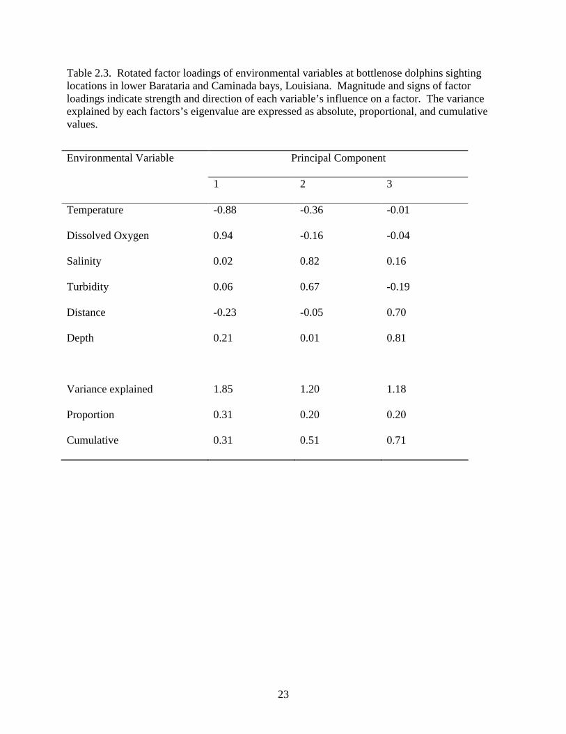
The PCA resolved the six environmental variables into three orthogonal factors that
explained 71 % of the variability of the data set (Table 2.3). The first three components had
eigen values greater than one. Each of the six environmental variables loaded heavily on at least
one factor. Factor 1 accounted for 30 % of the variability. Heavy loadings were apparent for
temperature and dissolved oxygen yet signs were opposite and reflect the seasonal patterns of
temperature and dissolved oxygen evident in the study area. Factors 2 and 3 each accounted for
an additional 20 % of the variability. Factor 2 loaded strongly on both salinity and turbidity.
Salinity decreases as distance from Gulf waters increases, which in this case represents
progressively more northern areas. However, there is also semi-annual variability in salinity
values. Higher turbidity rates occur in water close to the shore and in more frequently or
recently disturbed waters. Strong positive loadings for distance from shore and depth were
evident in Factor 3. Distance from shore was greatest in open waters areas north of Grande Isle
and Grande Terre where wetland areas were absent. Though depth was relatively homogenous
throughout the study area, channels and passes were deeper. Distance from shore and water
depth described a spatial three-dimensional component of the coastal landscape.
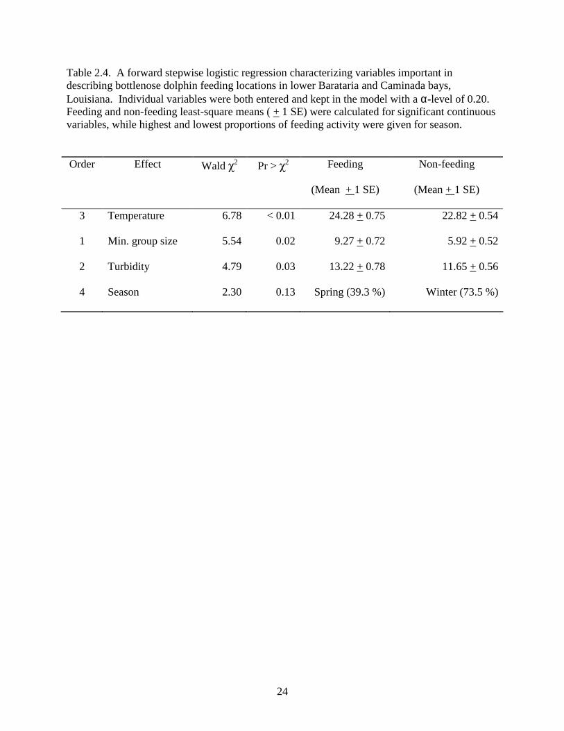
Foraging behavior was evident in 88 of the 269 sightings during this study. A forward
stepwise logistic regression selected four environmental variables to describe feeding sites in the
following order: minimum group size, turbidity, temperature, and season (Table 2.4).
Multicollinearity was not a problem as evidenced by a mean VIF value of 1.74, with no
individual VIF value exceeding 5. None of the selected variables were later discarded as a result
of the stepwise procedure. The Hosmer and Lemeshow criterion found the selected model to be
23
Table 2.3. Rotated factor loadings of environmental variables at bottlenose dolphins sighting locations in lower Barataria and Caminada bays, Louisiana. Magnitude and signs of factor loadings indicate strength and direction of each variable’s influence on a factor. The variance explained by each factors’s eigenvalue are expressed as absolute, proportional, and cumulative values.
Environmental Variable Principal Component
1 2 3
Temperature -0.88 -0.36 -0.01
Dissolved Oxygen 0.94 -0.16 -0.04
Salinity 0.02 0.82 0.16
Turbidity 0.06 0.67 -0.19
Distance -0.23 -0.05 0.70
Depth 0.21 0.01 0.81
Variance explained 1.85 1.20 1.18
Proportion 0.31 0.20 0.20
Cumulative 0.31 0.51 0.71
24
Table 2.4. A forward stepwise logistic regression characterizing variables important in describing bottlenose dolphin feeding locations in lower Barataria and Caminada bays, Louisiana. Individual variables were both entered and kept in the model with a α-level of 0.20. Feeding and non-feeding least-square means ( + 1 SE) were calculated for significant continuous variables, while highest and lowest proportions of feeding activity were given for season.
Order Effect Wald χ2 Pr > χ2 Feeding
(Mean + 1 SE)
Non-feeding
(Mean + 1 SE)
3 Temperature 6.78 < 0.01 24.28 + 0.75 22.82 + 0.54
1 Min. group size 5.54 0.02 9.27 + 0.72 5.92 + 0.52
2 Turbidity 4.79 0.03 13.22 + 0.78 11.65 + 0.56
4 Season 2.30 0.13 Spring (39.3 %) Winter (73.5 %)
25
a reasonable fit to the data (χ82 = 5.79, p = 0.67). Minimum group size, turbidity and
temperature were all higher in feeding versus non-feeding observations. The incidence of
feeding was highest in spring (39.3 %) and lowest in winter (26.5 %).
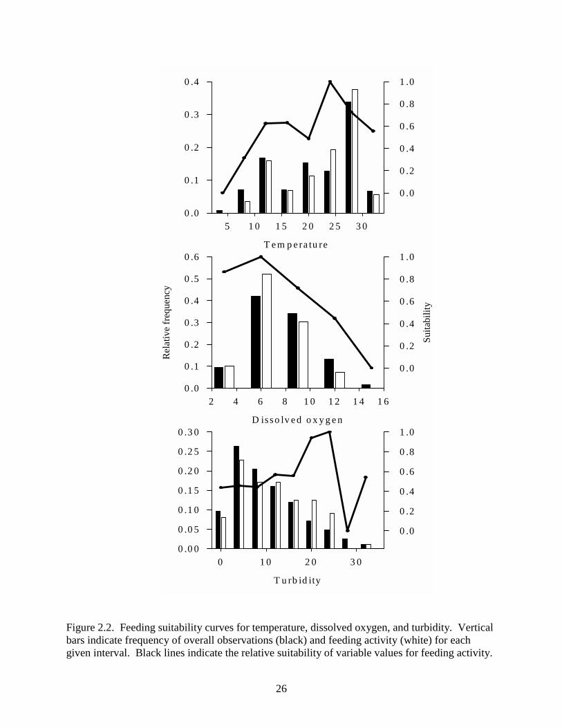
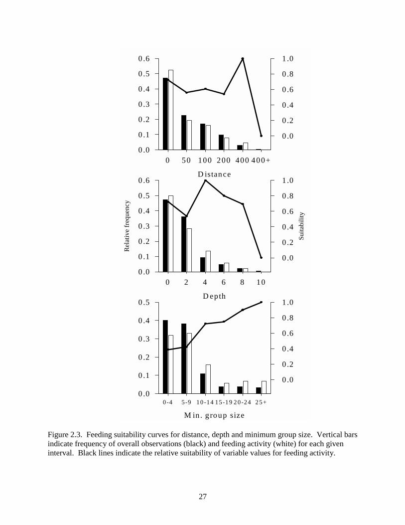
Feeding habitat suitability curves indicated selection patterns for temperature, turbidity,
distance from shore, depth and minimum group size. Selected temperatures for feeding were
between 20 and 24 °C (Figure 2.2). Dissolved oxygen content selection peaked around 6 mg/L
and declined as values increased (Figure 2.2). Salinity selection results were somewhat
ambiguous due to a small number of observations for the lowest interval of salinity values that
acted to inflate the associated S value. However, there was a small peak around 20 psu. Feeding
selection was pronounced for turbidity values between 20 and 28 NTU (Figure 2.2). Though a
majority of observations were made in waters less than 50 m from shore, a selection for waters
between 200 and 500 m from shore was apparent (Figure 2.3). Selection for feeding was highest
in water depths between 4 – 6 m of water (Figure 2.3). There was a steady climb in proportion
of feeding observations as minimum group size increased (Figure 2.3). There appeared to be no
obvious pattern relating time of day with feeding activity. Environmental variables that were
identified as important descriptors of feeding activity in the logistic regression analysis (i.e.,
minimum group size, temperature, turbidity and season) showed selection for feeding activity in
extreme values of the resource availability, rather than mid-range values. For example,
temperature and turbidity showed pronounced selection values for higher values (Figure 2.2) and
as minimum group size increased so did relative feeding suitability (Figure 2.3). However, depth
(Figure 2.3) and dissolved oxygen (Figure 2.2) showed relatively strong suitability in mid-range
values yet were not selected in the logistic regression analysis.
GIS maps of feeding versus non-feeding sites identified areas (Figure 2.4) where feeding
26
T e m p e ra tu re
5 1 0 1 5 2 0 2 5 3 00 .0
0 .1
0 .2
0 .3
0 .4
0 .0
0 .2
0 .4
0 .6
0 .8
1 .0
D is so lv e d o x y g e n
2 4 6 8 1 0 1 2 1 4 1 6
Rel
ativ
e fr
eque
ncy
0 .0
0 .1
0 .2
0 .3
0 .4
0 .5
0 .6
Suita
bilit
y
0 .0
0 .2
0 .4
0 .6
0 .8
1 .0
T u rb id ity
0 1 0 2 0 3 00 .0 0
0 .0 5
0 .1 0
0 .1 5
0 .2 0
0 .2 5
0 .3 0
0 .0
0 .2
0 .4
0 .6
0 .8
1 .0
Figure 2.2. Feeding suitability curves for temperature, dissolved oxygen, and turbidity. Vertical bars indicate frequency of overall observations (black) and feeding activity (white) for each given interval. Black lines indicate the relative suitability of variable values for feeding activity.
27
M in . g roup size
0-4 5-9 10-14 15-19 2 0-24 2 5+0 .0
0 .1
0 .2
0 .3
0 .4
0 .5
0 .0
0 .2
0 .4
0 .6
0 .8
1 .0
D istance
0 50 100 200 400 400+0 .0
0 .1
0 .2
0 .3
0 .4
0 .5
0 .6
0 .0
0 .2
0 .4
0 .6
0 .8
1 .0
D epth
0 2 4 6 8 10
Rela
tive
freq
uenc
y
0 .0
0 .1
0 .2
0 .3
0 .4
0 .5
0 .6
Suita
bilit
y
0 .0
0 .2
0 .4
0 .6
0 .8
1 .0
Figure 2.3. Feeding suitability curves for distance, depth and minimum group size. Vertical bars indicate frequency of overall observations (black) and feeding activity (white) for each given interval. Black lines indicate the relative suitability of variable values for feeding activity.
28
#S
##S
#S
#S
#
#
#S#S
#S
#S
#S#
#S#
##S
##S#
#S
#S#S
#S#
#S # #
#S
#S
#S
#S
#S
#S #S
#
#S
#
#
#
#
#
#
#
#
#
#
#
#S
#S
#S
#S#S #S
#S
#
#S
#
#S
#S
##
#
##
#S
###
#S
#S
#
#
#S #S#S#S
#S#S
#S
#
#S#S#
#S
#
# ##S##
#S#S#
#S
#S#S
#S#S
#S #S
#S##S
#S
## #S
#S
#S
#S##S
#S
#
#S#S
#S#S
#
#S
##S
#S
#S
#S#S
#S #S#S
#S#S
#S
#S
#S
#S#S
#
#S#
##S
#S
#S
#S#S#S
#
#
#
##S
#
#S
#S
#
#S
#
#S
#S#S
#
#S
#S#
#
#S
#
#S
#S
#S
#
#
#S
#
#
#S
#S
#S#S#S
#S
#S ##S #S
#S#S
#S
#
##S
#S#S
#S
#S
#
#S#S #S #S
#S#S
#S#S
#S
#S#S#S
#
#S
#S
#
#S
#S
#S
#S
#S
#S#S
#S#
##
#S
#S#S
#
#
##S
#
#S#S
#S
##S
#S
#S
#S
#S
#S
#S
#
#S
#S#
#
#
#S
#S
#S #S
#S#S#
2 0 2 4 Miles
S
N
EW
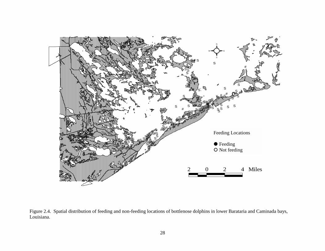
Figure 2.4. Spatial distribution of feeding and non-feeding locations of bottlenose dolphins in lower Barataria and Caminada bays, Louisiana.
Feeding Locations � Feeding � Not feeding
29
activity was relatively high. More than 50% of the observations in waters directly around the
Caminada Pass area involved feeding activity. The northeastern ends of both Grande Isle and
Grande Terre had relatively high rates of feeding also, but only a small number of observations
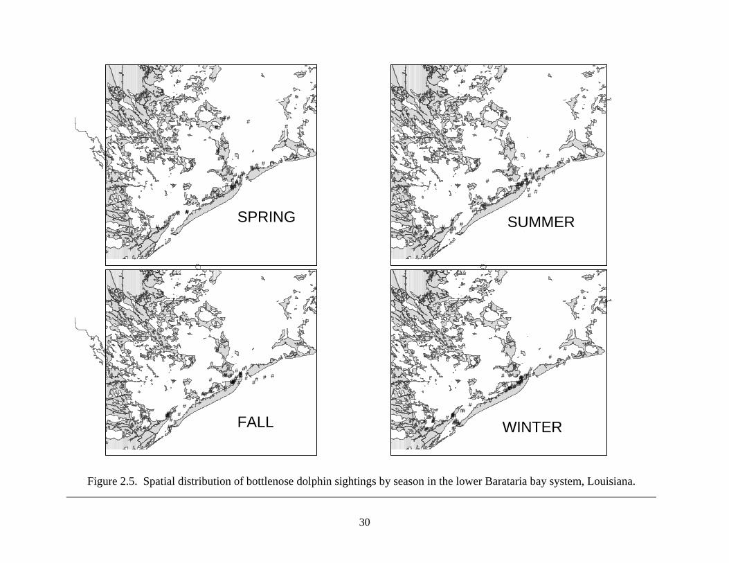
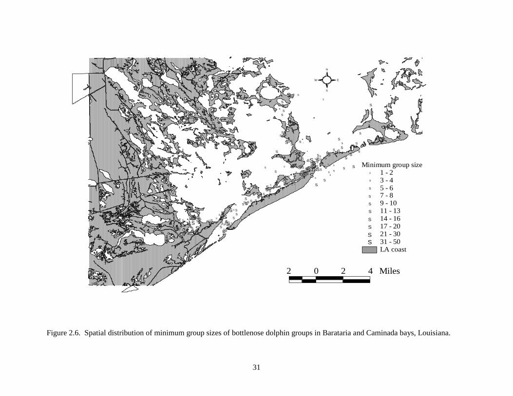
were made in these areas. Projections of minimum group size estimates and seasonal
distribution of sighting locations showed a general pattern of larger group sizes in the passes
(Figure 2.5). Distribution range in summer was more expansive, yet these findings are heavily
confounded by weather conditions that prohibited surveys in some regions during colder months
(Figure 2.6).
DISCUSSION
This study utilized a fine-scale approach to examine patterns in bottlenose dolphin
distribution, habitat use and feeding activity. Even though four of six measured environmental
variables were significantly different on a seasonal basis bottlenose dolphins were present during
all surveys conducted in the study area. Overall variability in environmental conditions were
driven by three sets of environmental variables (Table 2.3). Relationships between temperature
and dissolved oxygen, salinity and turbidity, and distance and depth represent variability on
seasonal, spatial-seasonal and spatial, scales respectively. Spatial distribution patterns within the
Barataria Basin showed general aggregation and feeding activity in the channels and passes, as
well as differences in the range of seasonal observations. Feeding sites were differentiated from
non-feeding sites by group size, temperature, turbidity and season in the logistic regression
(Table 2.4). Habitat selection analysis indicated that feeding was most common in waters 4 – 6
m deep, 200 – 500 m from shore with salinity values of around 20 psu (Figures 2.2 and 2.3).
30
##
####
##
## ##
#
##
#
##
##
#
#
# ####
###
#
##
## # #
###
### #
#
#
#
#
##
#
###
#
##
##
##
#
##
#
#
##
#
#
FALL
##
### # #
#
#
#
#
#
# #
#
#
##
#
#
#
#
#
#
###
#
#
#
#
##
#
#
##
##
#
#
#
#
#
##
#
#
#
#
#
###
# ##
###
SPRING
###
##
##
###
#
#
##
#
#
##
##
#
#
#
#
#
#
#
#
## #
#
#
#
#
#
#
##
#
##
#
# ## #
##
#
#
##
###
#
### ##
# #
##
#
###
#
SUMMER
#
##
###
#
#
###
##
#
##
#
###
#
##
# #####
#
#
#
##
#
##
##
#
#
###
#
#
#
##
#
#
#
###
#
#
#
#
#
#
#
##
#
#
#
#
WINTER
Figure 2.5. Spatial distribution of bottlenose dolphin sightings by season in the lower Barataria bay system, Louisiana.
31
#S
#S
#S
#S
#S
#S
#S
#S
#S#S
#S
#S
#S#S
#S
#S
#S#S
#S#S
#S
#S
#S#S#S
#S
#S#S
#S#S
#S#S
#S
#S
#S
#S
#S
#S
#S#S
#S
#S
#S
#S
#S
#S
#S
#S
#S
#S
#S
#S
#S
#S
#S
#S
#S#S #S
#S
#S
#S
#S
#S
#S
#S
#S
#S
#S
#S
#S
#S
#S#S
#S
#S
#S
#S
#S#S
#S#S
#S
#S
#S
#S
#S
#S
#S
#S
#S
#S#S
#S#S#S
#S#S#S
#S
#S#S
#S
#S#S #S
#S#S
#S
#S
#S#S
#S
#S
#S
#S
#S
#S
#S
#S
#S
#S#S
#S
#S
#S
#S#S
#S
#S
#S
#S
#S
#S#S
#S#S#S#S
#S #S
#S
#S
#S
#S#S
#S
#S#S
#S#S
#S
#S
#S#S#S
#S
#S
#S
#S
#S
#S
#S
#S
#S
#S
#S
#S
#S#S
#S
#S
#S#S
#S
#S
#S
#S
#S
#S
#S
#S
#S
#S
#S
#S
#S
#S
#S#S#S
#S
#S#S
#S #S
#S
#S
#S
#S
#S
#S
#S#S
#S
#S
#S
#S
#S#S
#S#S
#S
#S
#S
#S
#S#S
#S
#S
#S
#S
#S
#S
#S
#S
#S
#S
#S
#S
#S#S
#S#S
#S#S
#S
#S#S
#S
#S
#S
#S
#S
#S
#S
#S
#S
#S#S
#S
#S
#S
#S
#S
#S
#S
#S
#S
#S
#S
#S
#S
#S #S
#S#S
#S
2 0 2 4 Miles
S
N
EW
LA coast
Minimum group size#S 1 - 2#S 3 - 4#S 5 - 6#S 7 - 8#S 9 - 10#S 11 - 13#S 14 - 16#S 17 - 20#S 21 - 30#S 31 - 50
Figure 2.6. Spatial distribution of minimum group sizes of bottlenose dolphin groups in Barataria and Caminada bays, Louisiana.
32
Environmental Correlates with Marine Mammal Distribution
Environmental variables showed significant seasonal differences for temperature,
dissolved oxygen, salinity and turbidity (Table 2.2). The inverse correlation between
temperature and dissolved oxygen (Table 2.3) further indicated that seasonal differences play an
important role in describing the distribution and behavior patterns of bottlenose dolphins in the
Barataria basin. In addition, a logistic regression analysis noted that both season and
temperature were important in describing feeding locations (Table 2.4). Numerous relationships
between marine mammal distribution and seasonal trends have been detected. Commonly, the
driving force in these associations is temperature fluctuations. Short-beaked common dolphins
(Delphinus delphis) were found to move to inshore New Zealand waters during summer and
spring (Neumann 2001). The occurrence of pronounced inshore movement during La Niña
emphasized the correlation between warmer waters and inshore spatial distribution. In proximal
waters, sea surface temperature was found to be a decisive factor in distribution limits of four
species of Delphinidae (Gaskin, 1968). Similarily, Au and Perryman (1985) reported that
spotted (Stenella attenuata) and spinner dolphins (Stenella longirostris) were abundant in
tropical surface waters of relatively stable temperatures whereas common and striped dolphins
showed preference for more variable equatorial and subtropical waters. However, these winter
observations differed slightly from Reilly’s (1990) findings for the same region during summer
months. The two sub-groupings remained, though striped (Stenella coerulealba) and common
(Delphinus delphis) dolphins became spatially separated in warmer months. In some studies,
density differences in abundance have been observed on a seasonal basis. Tershy et al. (1990)
found seasonal patterns to the presence of Fin (Balaenoptera physalus) and Bryde’s
(Balaenoptera edeni) whales within the Gulf of California, Mexico. The frequency of both
33
species was negatively correlated with temperature. Hector’s dolphins (Cephalorhynchus
hectori) showed seasonal offshore movement (Dawson and Slooten 1988) though smaller scale
diurnal observations have been inconsistent (Stone 1995, Bejder and Dawson 2001). In southern
Texas there was a peak in winter abundance estimates of bottlenose dolphins (Shane 1980).
However, no apparent relationship exists between season and the frequency distribution of births
for the same species in the Gulf of Mexico (Urian et al. 1996).
It is a common contention that environmental variables associated with feeding activities
may be proxies for the abundance or availability of important prey species (Kenney and Winn
1985, Selzer and Payne 1988). Specifically, either the distribution pattern or the preferred
habitat of common prey species may be the determining factor. Salinity and turbidity were
important in describing environmental variability in my study (Table 2.3) and also play
important roles in distributing and providing refugia for bottlenose dolphin prey from most other
predators. The former is a major determinant of community structure in estuaries and the latter
reduces detection from visual nekton predators. The observed relationship between salinity and
turbidity indicate the importance of both spatial and temporal components. The importance of
additional spatial variables (i.e., depth and distance from shore) may be due to benefits related to
prey capture or congregation. A logistic regression analysis (Table 2.4) determined that
minimum group size, temperature, turibidity and season were all significant in describing feeding
versus non-feeding locations. In addition habitat suitability curves (Figures 2.2 and 2.3) were
able to define ranges of each specific environmental variable where feeding activity appeared to
be most likely. These findings are unique in that most often a higher or lower scale of selection
is presented. Several other marine mammal research findings indicate that particular
environmental variables may be important indicators of prey species’ distribution patterns.
34
One of the distinctions between the resident and transient killer whales (Orcinus orca) of
the Pacific Northwest (Olesiuk et al. 1990, Hoezel 1993, Saulitis et al. 2000) is their primary
prey choice of fish and marine mammals, respectively. These two prey choices utilize different
features of bottom topography, and consequently the distribution patterns of resident and
transient killer whale pods parallel these features. In Sarasota Bay, western Florida, Barros and
Wells (1998) found that stomach contents of bottlenose dolphins suggest an expected correlation
between prey habitat and dolphin foraging areas. Group sizes of spotted, spinner and common
dolphins in the eastern Pacific Ocean were observed to mirror the diurnal group size fluctuations
of yellowfin tuna, one of their common prey items (Scott and Cattanach 1998). Au and
Perryman (1985) had documented, but not directly quantified, these associations over a decade
earlier. In an extension to this work, Au and Pitman (1986) found positive statistical
relationships between bird flocks and spinner and spotted dolphin schools. Pilchard movements
up the eastern coast of South African coast have been accompanied by migration of common
dolphins during winter months (Cockroft and Peddemors 1990). Sperm whale (Physeter
macrocephalus) frequency is significantly greater on the eastern boundary of a Gulf Stream
warm-core ring off Georges Bank (Griffin 1999). Entrainment of shelf waters within the warm-
core ring is believed to provide suitable habitat for common prey items of sperm whales. Selzer
and Payne (1988) found seasonal variation in sea surface temperatures and salinities for white-
sided and common dolphins, and hypothesized that the interactions of these factors with sea floor
topography and associated upwelling may be responsible for aggregating prey. In Belize,
dolphins were most consistently observed at the interface between the open ocean and more
protected sea-grass beds and mangrove shorelines of the Turneffe Atoll (Grigg and Markowitz
1997). This interface is often recognized as a highly productive region that may also act as a
35
nursery for juvenile fishes. Interestingly, protected central lagoon sites and creek mouths were
frequented least. Quiescent waters may not be conducive to prey capture, as tidal movement has
been associated with feeding in several studies (Shane 1980, Gregory and Rowden 2001). In the
Gulf of California, Ballance (1992) found sighting rates and feeding activities of bottlenose
dolphins to be significantly greater in areas less than 5.5 km from productive estuarine areas.
Within the Sado Estuary, Portugal, Harzen (1998) noted that specific sub-areas of the estuary
appeared to be used for certain activities. Foraging was observed throughout the entire study
area, although it was most prominent in areas close to openings from the estuary to open waters.
Katona and Beard (1990) identified larger scale distinctions in feeding locations for humpback
whale populations of the North Atlantic. Five specific feeding locations and one major winter
breeding aggregation region were identified. Feeding behavior has sometimes been correlated
with increased group size (Shane et al. 1986). Campbell et al. (2002) suggested that larger
groups were more effective in searching for food and efficient in cooperative feeding strategy.
The logistic regression performed in my study concurred with this assertion (Table 2.4). Both
Corkeron (1990) and (Grigg and Markowitz 1997) identified both food patchiness and inter-
specific interactions as important influences on Tursiops group size. Alternatively, for the same
species in Cardigan Bay, West Wales, group size was unrelated to foraging activity (Gregory and
Rowden 2001).
However, not all cetacean feeding behavior is predictable. Hoezel et al. (1989) found that
individual minke (Balaenoptera acutorostrata) whales adopted specialized foraging strategies in
similar oceanographic regimes. Individual foraging techniques were believed to be a product of
learned behaviors. Bottlenose dolphins are both flexible and opportunistic in their feeding
activity (Shane et al. 1986). In Shark Bay, Western Australia, a small number of individuals
36
have been observed carrying sponges on their rostra as what is believed to be a foraging tool
(Smolker et al. 1997). Observations of feeding in association with shrimp boats have been
documented in Texas waters (Leatherwood 1975, Brager 1993) and feeding on mud-banks by
partial beaching has been observed in some salt-marsh areas (Hoese 1971).
Innovative approaches to establishing habitat usage patterns, behavior budgets and
movement patterns of marine mammals have been achieved by such methods as outfitting adult
male seals with video cameras (Parrish et al. 2000), attaching satellite-monitored radio tags to
large whales (Lagerquist et al. 2000), and using GIS to establish spatio-temporal prediction
models (Hamazaki 2002). Besides the limited time for data collection, video and satellite-tags
require direct implementation and proximity to individuals that often results in small sample
sizes. Prediction models attempt to assess habitat suitability of areas where current survey data
is not available. However, the usefulness of these models is dependent on the quality, range and
resolution of data available for analysis. Recently Brager et al. (2003) was able to assess
preferences of Hector’s dolphin by measuring sea-surface temperature, water depth and water
clarity at both used and unused sites. This study found significant relationships between all three
variables both individually and when combined, though preferences varied by region and season.
Measurements on additional environmental variables would undoubtedly provide added insight
into the ecology of this species.
Survey Design
The seasonal pattern of spatial distribution in bottlenose dolphin sighting locations is
strongly influenced by environmental conditions that may limit survey efforts. DeMaster et al.
(2001) found that Beaufort Sea state 1 conditions increased the probability of sighting beluga
whales. Therefore, observed seasonal differences in density may be due to inclement weather

37
conditions rather than movement of individuals out of a given area. In this study, I found that
Beaufort Sea state conditions were lower in summer and spring. Due to the variability in
seasonal weather conditions it was difficult to quantify differences in spatial patterns of feeding,
seasonal observations and minimum group size (Figures 2.4, 2.5 and 2.6). Forney et al. (1991)
were able to address this issue by incorporating environmental conditions as a covariate into their
modeling efforts of harbor porpoises. Another issue when conducting survey work is the ability
to detect groups with equal probability. It is likely that a positive bias results from the higher
probability of sighting larger groups exhibiting more acrobatic activities. If there is
inaccessibility of regions due to poor conditions that cause a non-representative sample of the
environment or behavior to occur, the reported results may also be biased.
Conservation
Two bottlenose dolphin stocks meet at the interface of Barataria Bay and the Gulf of
Mexico (Waring et al. 2002). The distribution limits of the western Gulf of Mexico (wGOM)
bottlenose dolphin stock extend from presumed bay boundaries to the 18.3 m isobath all the way
from the Texas border to the Mississippi River mouth. Approximately 3500 individuals are
estimated to constitute the wGOM stock. The Barataria Bay “community” (see Wells et al.
1987, Waring et al. 2002) is believed to be about 219 individuals though recent work indicates
that this may be an overestimate (C. Miller, Chapter IV). Distinctions between these two stocks
are based in part on the assumption that movements between stock regions are limited by
dissimilar climates and oceanographic conditions. In accordance with these assumed population
boundaries and different marine environments the Barataria bay stock is managed separately
from the wGOM under the Marine Mammal Protection Act.
38
CONCLUSIONS
Though many researchers have investigated environmental correlates in relation to
marine mammal distribution or activities, the assessment of a synchronous suite of
environmental forcing factors of bottlenose dolphin populations has been limited. Furthermore,
the observed relationships between bottlenose dolphin distribution and behavior represent
selection of environmental conditions, but should not be interpreted to indicate actual
preferences (Baltz 1990). In an effort to provide a representative sample I used a randomly
stratified survey design. The amount of effort I was able to devote to this project was limited by
factors such as weather conditions, time constraints and size of the research vessel. Regardless I
feel that the observations made during this study constitute a satisfactory and meaningful dataset
describing environmental usage patterns of bottlenose dolphins in the area. A spatially and
temporally explicit fine-scale characterization of the area would allow more definitive
conclusions regarding bottlenose dolphin preference of environmental variables in this area. In
addition there are many more variables that could be included in a habitat characterization.
These factors may include but are not limited to tidal stage, chlorophyll a concentration,
movement of prey, presence of predators or competitors, water velocity and age composition of
groups. Despite these considerations, my findings with regard to habitat usage findings were
able to effectively determine both the range and variance of important environmental variables
and highlight strong variable selection for bottlenose dolphins in this region. Though the exact
reasons for observed habitat selection are elusive, the development and quantification of an
environmental context for population activity, movement, behavior, and residency patterns is an
39
interesting step towards protecting individual populations and predicting future patterns of
habitat use in the event of environmental change.
LITERATURE CITED Allen, M. C. and A. J. Read. 2000. Habitat selection of foraging bottlenose dolphins in relation to boat density near Clearwater, Florida. Marine Mammal Science 16: 815-824. Allison, P. D. 1991. Logistic Regression using the SAS System: Theory and Application. SAS Institute Inc., Cary, North Carolina. Au, D. W. K. and W. L. Perryman. 1985. Dolphin habitats in the eastern tropical Pacific. Fishery Bulletin 83: 623-643. Au, D. W. K. and R. L. Pitman. 1986. Seabird interactions with dolphins and tuna in the Eastern Tropical Pacific. The Condor 88: 304-317. Ballance, L. T. 1992. Habitat use patterns and ranges of the bottlenose dolphin in the Gulf of California, Mexico. Marine Mammal Science 8: 262-274. Baltz, D. M. 1990. Chapter 18, Autecology. Pages 585-607 in Methods for Fish Biology. C. B. Shreck and P. B. Moyle (eds.). American Fisheries Society. Bethesda, Maryland. Baltz, D. M., J. W. Fleeger, C. F. Rakocinski, and J. N. McCall. 1998. Food, density, and microhabitat: factors affecting growth and recruitment potential of juvenile saltmarsh fishes. Environmental Biology of fishes 53: 89-103. Barros, N. B. and R. S. Wells. 1998. Prey and feeding patterns of resident bottlenose dolphins (Tursiops truncatus) in Sarasota Bay, Florida. Journal of Mammalogy 79: 1045-1059. Baumann, R. H, and R. E. Turner. 1990. Direct impact of the outer continental shelf activities on wetland loss in the central Gulf of Mexico. Environmental geology and water resources 15: 189-198. Bejder, L. and S. Dawson. 2001. Abundance, residency, and habitat utilisation of Hector’s dolphins (Cephalorhychus hectori) in Porpoise Bay, New Zealand. New Zealand Journal of Marine and Freshwater Research 35: 277-287. Blaylock, R. A. and W. Hoggard. 1994. Preliminary estimates of bottlenose dolphin abundance in southern U. S. Atlantic and Gulf of Mexico continental shelf waters. NOAA Technical Memorandum. NMFS-SEFCS-356, 10 pp. Brager, S. 1993. Diurnal and seasonal behavior patterns of bottlenose dolphins (Tursiops truncatus). Marine Mammal Science 9:434-438.
40
Brager, S., J. A. Harraway and B. F. J. Manly. 2003. Habitat selection in a coastal dolphin species (Cephalorhynchus hectori). Marine Biology 143:233-244. Breslin, P., N. Frunzi, E. Napoleon, and T. Ormsby. 1999. Getting to know ArcView GIS – the geographic information system (GIS) for everyone. ESRI Press, Redlands, California. Campbell, G. S., B. A. Bilgre and R. H. Defran. 2002. Bottlenose dolphins (Tursiops truncatus) in Turneffe Atoll, Belize: occurrence, site fidelity, group size and abundance. Aquatic Mammals 28: 170-180. Cockroft, V. G. and V. M. Peddemors. 1990. Seasonal distribution and density of common dolphins Delphinus delphis off the south-east coast of Southern Africa. South African Journal of Marine Science 9: 371-377. Conner, W. H. and J. W. Day, Jr. 1987. The ecology of Barataria Basin, Louisiana: an estuarine profile. U.S. Fish and Wildlife Service Biological Report 85 (7.13). 165 pp. Corkeron, P. J. 1990. Aspects of the behavioral ecology of inshore dolphins Tursiops truncatus and Sousa chinensis in Moreton Bay, Australia. Pages In S. Leatherwood and R. R. Reeves (eds.). The Bottlenose dolphin. Academic Press, Inc: San Diego, California, U.S.A. Dawson, S. and E. Slooten. 1988. Hector’s dolphin Cephalorhynchus hectori: distribution and abundance. Report of the International Whaling Commission (Special Report 9): 315- 324. Day, Jr. J. W., C. A. S. Hall, W. M. Kemp and A, Yáñez-Arancibia. 1989. Estuarine Ecology. John Wiley and Sons, New York. Day, Jr. J. W., D. Pont, P. F. Hensel and C. Ibanez. 1995. Impacts of sea-level rise on deltas in the Gulf of Mexico and the Mediterranean: The importance of pulsing events to sustainability. Estuaries 18: 636-647. DeMaster, D. P., L. F. Lowry, K. J. Frost and R. A. Bengtson. 2001. The effect of sea state on estimates of abundance for beluga whales (Delphinapterus leucas) in Norton Sound, Alaska. Fishery Bulletin 99: 197-201. Duffield, D. A., S. H. Ridgeway and L. H. Cornell. 1983. Hematology distinguishes coastal and offshore forms of dolphins (Tursiops). Canadian Journal of Zoology 61: 930-933. Duffield, D. A. and R. S. Wells. 1986. Population structure of bottlenose dolphins: Genetic studies of bottlenose dolphins along the central west coast of Florida. Contract report to NMFS SEFSC, Contract No. 45-WCNF-5-00366, 16 pp.
41
Forney, K. A., D. A. Hanan and J. Barlow. 1991. Detecting trends in harbor porpoise abundance from aerial surveys using analysis of covariance. Fishery Bulletin 89: 367- 377. Freund, R. J. and W. J. Wilson. 1997. Statistical Methods, Academic Press, N.Y. Garrison, T. 1999. Oceanography: an introduction to Marine Science (3rd Edition). Wadsworth Publishing Company, Belmont, California, U.S.A. Gaskin, D. E. 1968. Distribution of Delphinidae (Cetacea) in relation to sea-surface temperatures off eastern and southern New Zealand. New Zealand Journal of Marine and Freshwater Research 2: 527-534. Gregory, P. R. and A. A. Rowden. 2001. Behaviour patterns of bottlenose dolphins (Tursiops truncatus) relative to tidal state, time-of-day, and boat traffic in Cardigan Bay, West Wales. Aquatic Mammals 27: 105-113. Griffin, R. B. 1999. Sperm whale distributions and community ecology associated with a warm- core ring off Georges Bank. Marine Mammal Science 15: 33-51. Grigg, E. and H. Markowitz. 1997. Habitat use by bottlenose dolphins (Tursiops truncatus) at Turneffe Atoll, Belize. Aquatic Mammals 23: 163-170. Hamazaki, T. 2002. Spatiotemporal prediction models of cetacean habitats in the mid-western North Atlantic Ocean (from Cape Hatteras, North Carolina, U.S.A. to Nova Scotia, Canada). Marine Mammal Science 18:920-939. Harzen, S. 1998. Habitat use by the bottlenose dolphin (Tursiops truncatus) in the Sado Estuary, Portugal. Aquatic Mammals 24: 117-128. Hoese, H. D. 1971. Dolphin feeding out of water in a salt marsh. Journal of Mammalogy 52: 222-223. Hoezel, A. R. 1993. Foraging behavior and social group dynamics in Puget Sound killer whales. Animal Behavior 45: 581-591. Hoezel, A. R., E. M. Dorsey, S. J. Stern. 1989. The foraging specializations of individual minke whales. Animal Behavior 38: 786-794. Hurlbert, S. H. 1981. A gentile depilation of the niche: Dicean resource sets in resource hyperspace. Evolutionary Theory 5:177-184. Katona, S. K. and J. A. Beard. 1990. Population size, migrations and feeding aggregations of the humpback whale (Megaptera novaeangliae) in the western North Atlantic Ocean. Report to the International Whaling Commission (Special Issue) 12: 295-305.
42
Kenney, R. D. and H. E. Winn. 1986. Cetacean high-use habitats of the northeast United States continental shelf. Fishery Bulletin 84: 345-357. Lagerquist, B. A., K. M. Stafford and B. R. Mate. 2000. Dive characteristics of satellite- monitored blue whales (Balaenoptera musculus) off the central California coast. Marine Mammal Science 16: 375-391. Leatherwood, S. 1975. Some observations of feeding behavior of bottlenosed dolphins (Tursiops truncatus) in the northern Gulf of Mexico and (Tursiops cf. T. gilli) off southern California, Baja California, and Nayarit Mexico. Marine Fisheries Review 37: 10-16. Longley, P. A., M. F. Goodchild, D. J. Maguire and D. W. Rhind. 2001. Geographic Information systems and science. John Wiley and Sons, Ltd., West Sussex, England. Neumann, D. R. 2001. Seasonal movements of short-beaked common dolphins (Delphinus delphis) in the north-western Bay of Plenty, new Zealand: influence of sea-surface temperature and El Nino/La Nina. New Zealand Journal of Marine and Freshwater Research 35: 371-374. Olesiuk, P. F., M. A. Bigg and G. M. Ellis. 1990. Life history and population dynamics of resident killer whales (Orcinus orca) in the coastal waters of British Columbia and Washington state. Report to the International Whaling Commission (Special Issue 12): 209-243. Ormsby, T., E. Napoleon, R. Burke, C. Groessl and L. Feaster. 2001. Getting to know ArcGIS desktop. ESRI Press, Redlands, California. Parrish, F. A., M. P. Craig, T. J. Ragen, G. J. Marshall and B. M. Buhleier. 2000. Identifying diurnal foraging habitat of endangered Hawaiian monk seals using a seal-mounted video camera. Marine Mammal Science 16: 392-412. Reed, D., ed. 1995. Status and trends of hydrologic modification, reduction in sediment availablity and habitat loss/modification in the Barataria-Terrebonne estuarine system. Barataria-Terrebonne National Estuary Program (Publication #20). 338pp. Available from Barataria-Terrebonne National Estuary Program Office, Nicholls State University Campus, P.O. Box 2663, Thibodeaux, LA 70310. Reilly, S. 1990. Seasonal changes in distribution and habitat differences among dolphins in the eastern tropical Pacific. Marine Ecology Progress Series 66: 1-11. SAS Institute, 1996. SAS/STAT guide for personal computers. Version 6 edition. SAS Institute, Inc., Cary, North Carolina.
43
Saucier, M. H. and D. M. Baltz. 1993. Spawning site selection by spotted seatrout (Cynoscion nebulosus) and black drum (Pogonias cromis) in Louisiana. Environmental Biology of Fishes 36: 257-272. Saulitis, E., C. Matkin, L. Barrett-Lennard, K. Heise, G. Ellis. 2000. Foraging strategies of sympatric killer whales (Orcinus orca) populations in Prince William Sound, Alaska. Marine Mammal Science 16: 94-109. Scott, M. D. and K. L. Cattanach. 1998. Diel patterns is aggregations of pelagic dolphins and tunas in the eastern Pacific. Marine Mammal Science 14: 401-428. Selzer, L. A. and P. M. Payne. 1988. The distribution of white-sided (Lagenorhynchus acutus) and common dolphins (Delphinus delphis) vs. environmental features of the continental shelf of the northeastern United States. Marine Mammal Science 4: 141-153. Shane, S. H. 1980. Occurrence, movements, and distribution of bottlenose dolphin, Tursiops truncatus, in southern Texas. Fishery Bulletin 78: 593-601. Shane, S., R. S. Wells and B. Wursig. 1986. Ecology, behavior, and social organization of the bottlenose dolphin: a review. Marine Mammal Science 2: 34-63. Smolker, R., A. Richards, R. Connor, J. Mann and P. Berggren. 1997. Sponge carrying by dolphins (Delphinidae, Tursiops sp.): A foraging specialization involving tool use? Ethology 103: 454-465. Stone, G. 1995. Diurnal movement patterns of Hector’s dolphin as observed from clifftops. Marine Mammal Science 11: 395-402. Tershy, B. R., D. Breese and C. S. Strong. 1990. Abundance, seasonal distribution and population composition of balaenopterid whales in the canal de ballenas, Gulf of California, Mexico. Report to the International Whaling Commission (Special Issue 12): 369-375. Turner, R. 1997. Wetland loss in the northern Gulf of Mexico: multiple working hypotheses. Estuaries 20: 1-13. Urian, K. W. and R. S. Wells. 1996. Bottlenose dolphin photo-identification workshop. NOAA Technical Memorandum NMFS-SEFSC-393. Urian, K. W., D. A. Duffield, A. J. Read, R. S. Wells and E. D. Shell. 1996. Seasonality of reproduction in bottlenose dolphins, Tursiops truncatus. Journal of Mammalogy 77:394- 403. Waring, G.T., J.M. Quintal and C.P. Fairfield (Editors). 2002. U.S. Atlantic and Gulf of Mexico marine mammal stock assessments. NOAA Technical Memorandum NMFS-NE-169. vii + 180 + 4 app.

44
Wells, R. S., M. D. Scott and A. B. Irvine. 1987. The Social Structure of Free-ranging Bottlenose Dolphins. Pages 247-305 in H. Genoways, ed. Current Mammalogy Vol. 1. 519pp.
Wursig, B and M. Wursig. 1977. The photographic determination of group size, composition, and stability of coastal porpoises (Tursiops truncatus). Science 198: 755-756.

45
CHAPTER III
ASSESSMENT OF JOLLY-SEBER ASSUMPTIONS FOR NATURALLY MARKED CETACEAN PHOTO-IDENTIFICATION DATA
INTRODUCTION
Field research on cetaceans is often hampered by highly mobile subjects, limited number
of opportunities for visible contact, and heterogeneity of both oceanographic and climatic
conditions. In response to these difficulties, survey design and thorough analysis has sometimes
been ignored in lieu of capitalizing on scant opportunities to directly observe study animals.
Consequently, general and simplified models may be employed to estimate demographic
parameters. This may be necessary when assumptions of more complicated models cannot be
assessed or met. However, these circumstances may result in highly variable estimates with
intractable bias.
Photo-identification (photo-ID) techniques (Wursig and Wursig 1977, Olesiuk et al.
1990, Wursig and Jefferson 1990, Wells 1991) are frequently used to estimate demographic
parameters of marine mammals. An appropriate photo-ID survey design is determined by a
combination of factors including randomness requirements, weather conditions, behavior, and
vessel restrictions. Independent observers scan the water for individuals or groups once
underway. If sighted, the subjects are approached within a distance suitable for taking
photographs given existing weather conditions. Markings suitable for photo-ID are then
photographed for as many individuals as possible. Natural markings used in marine mammal
studies include nicks and notches on the dorsal fins (Wursig and Wursig 1977, Wells 1991),
saddle patch patterns (Baird and Stacey 1988, Olesiuk et al. 1990), pigmentation and markings
on tail flukes (Whitehead and Waters 1990) and callosity patterns on the rostrum (Bannister
1990, Payne et al. 1990). These distinctive features are assumed to be sufficiently long lasting,

46
slow in changing and unique enough to be recognized in subsequent sightings. Survey effort is
resumed once photo-ID efforts are complete or individuals vacate the area. After completion of
fieldwork, clear and complete images of the natural markings are examined for photographic
quality and relative distinctiveness. Records are then analyzed to describe patterns on the
appearance of new individuals, re-sighting frequencies, association patterns and distribution.
Application of mark-recapture statistical theory and models can be used on individual-sighting
histories to estimate population parameters. Mark-recapture model selection is dependent on the
population under study, the survey methodology employed, and several other associated
limitations or restrictions. Life history characteristics investigated have included population
dynamics (Best and Underhill 1990, Calambokidis et al. 1990b, Karczmarski et al. 1999), social
organization (Bigg et al. 1990, Whitehead 1990b), rates of survival (Buckland 1990) and
reproduction (Barlow 1990), sex and age ratios (Glockner-Ferrari and Ferrari 1990), site fidelity
(Wells and Scott 1990), movement patterns (Perkins et al. 1984, Calambokidis et al. 1990a) and
mortality (Wells and Scott 1990).
Many excellent reviews of the history, theory and development of mark-recapture
techniques, variously termed mark-and-recapture, capture-recapture, tag-recapture or band-
recovery, have been published (Seber 1992, International Working Group for Disease
Monitoring and Forecasting 1995, Schwarz and Seber 1999, Pollock 2000, Buckland et al. 2000).
Specific to wildlife studies, important summaries of both closed- (Otis et al. 1978, Chao 2001)
and open-population models (Pollock et al. 1990) have been prepared. Additionally, useful
books by Caughley (1977), Begon (1979) and Thompson et al. (1998) as well as two highly
influential editions of George Seber’s “The Estimation of Animal Abundance and Related
Parameters” (1973, 1982) are valuable contributors to the mark-recapture literature.
47
The starting point for mark-recapture methodology is commonly attributed to the
Lincoln-Petersen (L-P) estimator (Petersen 1896, Lincoln 1930). The L-P estimator assumes
there are no additions or deletions throughout the study duration, each individual has an equal
probability of being captured, and identifying marks are correctly documented and permanent.
For photo-ID studies, the terms capture and recapture can be used interchangeably with sighting
and re-sighting, respectively. The validity of the assumption of equal capture of individuals was
questioned and examined in an important monograph by Otis et al. (1978). Sources of variation
in individual capture can be attributed to capture response, temporal factors and inherent
individuality, that Otis et al. (1978) identified as possible sources of bias related to behavior,
time and heterogeneity, respectively. Behavior refers to a directional change in probability of
sighting after initial capture (i.e., either increased or decreased). Time accounts for temporally
dependent variables such as survey conditions, season and time of day. Heterogeneity suggests
that the uniqueness of any given individual will produce differences in probability of capture.
All possible combinations of these three sources of variation have been proposed. Models
describing individual heterogeneity have been the most difficult to characterize, though some
effectual solutions include jackknife estimators (Burnham and Overton 1978), mixture
distributions (Norris and Pollock 1996, Pledger 2000), explanatory covariates (Huggins 1989,
Alho 1990) and log-linear models (Cormack 1989). Chao (2001) reviewed and summarized
alternative solutions to the suite of Otis et al. (1978) models. The Otis et al. (1978) approach
was important for assessing closed population models, but populations that are geographically or
demographically open do not meet assumptions and require a different methodology.
In 1965, independent yet parallel descriptions of stochastic open-population model
notation, assumptions and methodology were published by G. M. Jolly and G. A. F. Seber (Jolly

48
1965, Seber 1965). More than two capture periods are required to estimate the size, survival or
recruitment rates of a population that may fluctuate due to birth, death, emigration or migration.
Marked individuals are linked to a specific survey date, though time between survey dates does
not need to be constant. Assumptions of the Jolly-Seber (J-S) model are that (1) every individual
in the population has the same probability of being captured in any given sample, (2) every
individual in the population has the same probability of survival, (3) the process of capture
places similar risks and fates on all individuals, (4) marks are recognized and accurately
identified on each sighting occasion, and (5) samples are instantaneous and all individuals are
released immediately after capture. Special cases of the J-S model include deaths only (Darroch
1959, Jolly 1965, Seber 1982), births only (Darroch 1959, Jolly 1965, Seber 1982), constant
survival and/or capture (Jolly 1982), age-dependent (Pollock 1981, Stokes 1984), cohort
(Buckland 1982, Seber 1982), and temporary trap response (Robson 1969, Pollock 1975,
Brownie and Robson 1983). Lebreton et al. (1992) continued the ideas of Pollock et al.’s (1990)
monograph by including strata such as sex, age, size and location. Seber (1982) suggests that a
minimum of ten re-sightings need to be seen on each capture occasion to avoid bias due to sparse
data.
Hammond (1986) initiated serious investigations into topics of mark-recapture analysis of
marine mammal photo-ID surveys. He stressed the need for proper implementation and
understanding of modeling strategies. This influential work resulted in the compilation of a
Special Issue of the International Report of the Whaling Commission (Hammond et al. 1990)
dedicated to matters relating to mark-recapture techniques for naturally marked marine
mammals. Individual contributions demonstrated the variety of applications and developments
that were underway in marine mammal investigations and also acknowledged the necessity of
49
assessing the appropriateness of model assumptions. The pivotal role of the J-S model in mark-
recapture theory for open-populations makes it a worthy candidate for investigating defensibility
of assumptions in regard to marine mammal photo-ID surveys. The objectives of this paper are
to interpret J-S model assumptions in the context of cetacean photo-ID studies and understand
the repercussions of possible violations of these assumptions.
BASIC MODEL ASSUMPTIONS
Each of the five J-S model assumptions were reviewed to discern the relevance of each
assumption within the context of cetacean photo-ID research. Crucial aspects for each
assumption were delineated to highlight the complexity and fine-scale obstacles that may arise
when determining the degree and direction of bias when a given assumption is violated.
Specifically, questions in regard to the validity of each assumption were examined to determine
whether it is a factor which may hamper the use of a traditional J-S model parameter estimate for
a given study population (Table 3.1).
(1) Every individual in the population has the same probability of being captured in any given
sample
For capture probabilities to be approximately equal, the sighting rate for each individual
must be similar. Detection of any given individual requires a number of particular events to be
satisfied in sequence. In photo-ID work the individual must be detected, the group or individual
must be approached within a distance suitable for image capture given the prevailing conditions,
and the identifying mark must be available for image capture. A necessary step to ensure equal
sighting rates is to randomize the survey protocol. Although the initial capture of animals may
be deliberate, subsequent recaptures (re-sightings) may not. However, as most photo-ID
research studies perform capture and recapture simultaneously, each survey must be random.
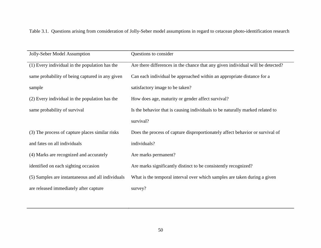
50
Table 3.1. Questions arising from consideration of Jolly-Seber model assumptions in regard to cetacean photo-identification research
Jolly-Seber Model Assumption Questions to consider
(1) Every individual in the population has the
same probability of being captured in any given
sample
Are there differences in the chance that any given individual will be detected?
Can each individual be approached within an appropriate distance for a
satisfactory image to be taken?
(2) Every individual in the population has the
same probability of survival
How does age, maturity or gender affect survival?
Is the behavior that is causing individuals to be naturally marked related to
survival?
(3) The process of capture places similar risks
and fates on all individuals
Does the process of capture disproportionately affect behavior or survival of
individuals?
(4) Marks are recognized and accurately
identified on each sighting occasion
Are marks permanent?
Are marks significantly distinct to be consistently recognized?
(5) Samples are instantaneous and all individuals
are released immediately after capture
What is the temporal interval over which samples are taken during a given
survey?
51
The random survey design must also ensure that neither location nor time of day is confounded.
Specifically, certain locations should not consistently be surveyed during similar times or in
predictable sequence. Another obvious, yet important consideration is that each population
member must be within the limits of the study area during surveys. If the population is
demographically open, the geographic range of the population must be known. The behavior and
size of the group at the time of sighting may affect the ability of researchers to see individuals.
For example, a large, acrobatic group is more easily visible than a few individuals quietly
milling. Particular behaviors may also be linked to such covariates as group size, time of day,
oceanographic features (such as tidal ebb or flow) and weather conditions. Although individuals
may be detected during one or more surveys, they might not ever be captured. Once an
individual is visible, it may simply ignore the vessel or react in manner that reduces the
probability of image capture. If an individual consistently avoids researchers, it may never be
captured. Avoidance behavior may be due to a previous experience or wariness. Alternatively,
individuals may intentionally approach the research vessel. Behavior may also be correlated
with distinctiveness of natural markings. For example, a positive response to boat traffic may
also result in more frequent interactions and greater probability of acquiring natural markings as
a result of interactions with vessels and gear. Additionally the age and experience of a calf may
directly affect its response to capture efforts. Given detection and appropriate proximity, it is
still not a certainty that an adequate image will be obtained. Surfacing behavior must allow the
naturally marked feature to be completely visible and presented at a satisfactory aspect for
photography. Covariates that are related to presentation, such as gender, age or size, may be
another source of heterogeneity in capture probability.

52
(2) Every individual in the population has the same probability of survival.
Survival estimates are calculated from marked individuals only. Therefore survival rates
for the entire population can be estimated only if survival rates for marked and unmarked
individuals are similar. However, if survey techniques are biased toward a particular gender or
age group resulting survival estimates may not be extended to the population without bias.
These skewed estimates may be a result of differential behavioral responses to surveys, unequal
probability of capture or relative distinctiveness of natural markings (see Assumptions 1 and 4).
Alternatively, survival estimates may be biased downwards if the capture process caused a
decline in fitness (see Assumption 3).
(3) The process of capture places similar risks and fates on all individuals
It is generally important to consider whether a capture episode may cause harm to an
individual by affecting behavior, health or social status. However, the non-invasive methods of
photo-ID do not pose serious risks to “captured” cetaceans. However, the proximity of research
vessels and plausible disruption to individuals’ activities requires consideration. This is
particularly true where researchers disrupt feeding, social, or reproductive activities. Behavioral
responses to the research vessel or changes in social affiliations as a result of photo-ID work may
cause heterogeneity in capture.
(4) Marks are recognized and accurately identified on each sighting occasion
Natural marking used for identification must persist throughout the duration of the study,
and must also be consistently recognizable on subsequent survey dates. When an individual is
incorrectly identified, the record of sighting histories obviously becomes inaccurate. The
frequency and trend in re-sightings is crucial in calculating demographic parameters and also
making determinations as to whether the population is closed or open. Population size estimates
53
will be biased if an individual is not consistently or accurately re-sighted during surveys. For
example, a distinctive mark that is only observable from one side reduces sighting probability by
one half.
(5) Samples are instantaneous and all individuals are released immediately after capture
This final assumption pertains to both total survey time as well as each individual
observation. Changes to a given population that occur while a single capture effort is being
performed will confound parameter estimates. If surveys are conducted over a relatively short
period this should not be a problem. However, over longer periods it may be unreasonable that
there are no demographic changes to the population. In photo-ID research individuals are
immediately returned to the population. Individual observation events are relatively brief in
nature. The underlying and general reason for Assumption 5 is to accurately define the study
population.
DISCUSSION
Close inspection of J-S assumptions in relation to photo-ID studies of naturally marked
cetaceans gave rise to several important themes crucial to ensuring the valid application of
models to cetacean populations. The most obvious and recurrent factor was the premise that all
samples and surveys are a representative subset of the entire population. Requirements include
being aware of the temporal and geographic range of the species and adhering to randomness
requirements. Larger scale random survey design also needs to be complemented by smaller
scale survey considerations. For example, image acquisition should be non-preferential, and
factors that may alter an individual’s probability of detection (i.e., group size, behavior or social
structure) must be taken into account. Natural markings used for individual identification need
to be reliable and recognizable. Finally, population parameter estimates need to be correctly
54
associated with an appropriate date or time period so that the population can be accurately
defined.
Open versus Closed Populations
An overwhelmingly crucial consideration in employing any type of mark-recapture
model is the initial evaluation of whether the population is open or closed. For representative
samples of the entire population, the first step is knowledge of the temporal and geographical
limits of the study population. There is no definitive test to determine whether a population is
open or closed, and so several researchers (e.g., Otis et al. 1978, Begon 1979) suggest that prior
experience and knowledge are the best guides for this determination. However, in a new
initiative or research into a rare species this premise may be dependent on the very research
about to be conducted. A priori information often aids in assessing a general core area of usage
by confirming consistent re-sightings of individuals within a survey region. A closed population
is assumed to have neither additions nor deletions within the temporal and spatial scale of the
study. This requires both biological (births and deaths) and geographical (immigration and
emigration) closure (Thompson et al. 1998). An open population allows movement into and out
of the study area, as well as births and deaths. Williams et al. (1993) analyzed the number of
new individuals sighted with accumulating effort to gauge whether they were encountering new
individuals or consistently seeing the same individuals (i.e., “Discovery Curve”). A steady and
asymptotic decrease in the number of new individuals discovered is often considered to represent
a closed population. Alternatively, a consistent increase in the number of sightings of marked
individuals may indicate an open population. In instances where the geographic range of the
population is not adequately covered the terminal slope of the Discovery Curve may be
misleading (Williams et al. 1993). This problem is particularly pronounced if the portion of the
55
population failing to be surveyed is a specific, non-random group. Implementation of an overall
random survey scheme is only assured when the complete geographic range of a population have
been assessed. Therefore, determination of whether a population is open or closed is crucial for
ensuring that: individual probabilities of capture are similar (Assumption 1), survival rates can
be approximately extended to unmarked individuals (Assumption 2), and that estimated
demographic parameters apply to a well-defined study population (Assumption 5).
Without a tremendously synchronous field effort it is rare that all samples for a given
survey will be conducted simultaneously. Often researchers violate J-S Assumption 5 as
logistics and capabilities of a field project do not permit a sufficient level of effort. Coordinated
research efforts were able to produce a North Atlantic ocean-basin-wide population estimate for
humpback whales (Smith et al. 1999). This multi-year study used standardized sampling and
analysis protocols over numerous study areas. Hammond and Thompson (1991) were able to
conduct a synchronous count of bottlenose dolphins present in Moray Firth, Scotland, though
mark-recapture techniques were not involved.
When the closure status of a population (i.e., open or closed) cannot be determined it may
be more appropriate to use an alternative method of abundance assessment. Indices denoting
relative trends in abundance have been developed with varying degrees of success for several
marine mammal species. Seasonal aerial surveys of endangered Florida manatee at warm-water
refugia were used as an index for total population size by application of a multiple regression
analysis with temporal components (Garrott et al. 1994), and later critically re-assessed with
independent life-history parameter estimates and non-linear modeling (Eberhardt et al. 1999).
However, beach counts of Hawaiian monk seals were an unreliable index for population size
(Eberhardt et al. 1999). Udevitz (1999) developed a parametric model to account for temporal
56
variability in index counts of Pacific Walrus. An alternative strategy to assessing abundance is
quantification of cetacean occupancy patterns within a specified geographic region (Durban et al.
2000).
A population may have periods of relative demographic stability punctuated by mortality,
breeding, immigration or emigration events. However, movement patterns of cetacean
populations are flexible. Emigration and immigration may occur with a fairly regular and
predictable temporal pattern (e.g., Humpback whales winter migration to Hawaii) involving
essentially all members of the population, though less predictable temporary emigration by only
a subset of individuals occurs also (e.g., Bottlenose dolphin males and transients in the Gulf of
Mexico). If a population’s movement patterns are relatively synchronous as in the former case,
it may be possible to conduct abundance estimates during times (and locations) of peak
abundance when minimal fluctuations in population occur. Less predictable temporary
emigration by only a selection of individuals occurs also. This second type of emigration has
recently received some specialized attention (Pradel et al. 1997). Disparate site-fidelity has been
observed in some estuarine bays adjoining the Gulf of Mexico (Wells et al. 1987, Maze and
Wursig 1999). So-called “residents” are individuals whose home range is consistently within a
bay region whereas “transients” exhibit more extensive ranging patterns and typically
intermingle and breed with nearby populations. Pollock et al. (1990) cited temporary emigration
as a serious source of bias. Likewise, Hammond (1990a) noted inconsistencies in blue whale
population estimates that he primarily attributed to movement patterns. Burnham (1993) has
shown how to account for random emigration. However, when emigration is permanent it is not
distinguishable from mortality. Whitehead (1990a) used a sperm whale example to demonstrate
that likelihood-ratio tests could be used to distinguish re-immigration, emigration and mortality.

57
However, sample size limitations of this technique may be problematic. Transients and residents
were separated in models designed by Pradel et al. (1997). These models assume resident
individuals behave similarly and that movement out of a region by transients is relatively
synchronous and for a known period of time.
Group and Individual Features That Effect Representative Samples
Even when geographic and temporal constraints of a given population are understood, the
finer-scale details of a sample need to be considered further. Differences in probability of
capture may be a result of individual characteristics and group associations or the immediate
environment. Factors such as age, gender, group size and activity may influence detectability.
The selection of only a sub-set of individuals for parameter estimates causes heterogeneity and
bias in capture probabilities (Assumption 1) and difficulties in determining how demographic
estimates can be extended to the entire population (Assumption 2). Some studies (e.g., Wells
and Scott 1990) have chosen to include only adults in population size estimates to lessen possible
age-related bias. Some models can assess age-related (Pollock 1981, Stokes 1984) or cohort-
specific survivorship (Seber 1982). However, it is not always possible to age or sex individuals
in the field. The well-documented social structure of many cetacean species (Bigg et al. 1990,
Weinrich 1991, Wells 1991) indicates that the probability of seeing one individual may be highly
related to the observance of other individuals. However, associations may be transitory (Connor
and Smolker 1995) or related to behavior, for e.g. feeding (Smith et al. 1981, Fertl and Wursig
1995, Rossbach 1999). Consequently sightings and missed observations may be clustered
(Cowan and Malec 1986). It is possible that either entire groups or individuals within a group
may be missed. Wilson et al. (1999) notes that more precise estimates may be produced when
non-independence of individuals in a population is taken into account. Whitehead (2001) found
58
both evidence and lack of support for heterogeneity when investigating within-group probability
of sightings for sperm whales. Behavior of the entire group may also affect sightability. Wade
and Gerrodettte (1993) noted that dolphins exhibiting more “showy” behaviors could be seen
from greater distances. Consistency in the presentation of features bearing natural markings
should also be considered. For example, Perkins et al. (1985) noted differences in fluke
presentation of discrete age classes. Whitehead (2001) found that younger sperm whales had
lower identification rates despite similar levels of natural markings. Stern et al. (1990)
investigated the efficiency with which individually identifiable minke whales could be
photographed. Surfacings were rated as “catchable” if both angle and distance from boat were
appropriate for image acquisition. Both the frequency and sequence of “catchable” surfacing
was quantified. Regions where minke whales were surveyed was found to be important in
describing these relationships as when behavior was more readily predictable, photographs were
attained more efficiently.
Surveys are often conducted in regions where recreational and commercial boats are
common. Frequent interaction with boats and proximity to human activities may cause
modifications to behavior (Assumption 1), increased risk of injury (Assumptions 2 and 3) and
anthropogenic pollution (Assumptions 2 and 3). A consistent response by all individuals to the
initial capture process is the behavioral response defined and accounted for in the Otis et al.
(1978) closed population models. However, it is unlikely that all individuals will behave in a
consistent manner. Both positive and negative responses to vessels have been documented for
various cetacean populations. Lesage et al. (1999) found that the vocal behavior of belugas in
the St. Lawrence River estuary are modified in response to ferries and small boats even though
these vessels regularly traverse the area. Collisions between large (> 80 m) ships traveling at
59
speeds greater than 14 knots is a serious (and often fatal) problem for large whales, including fin,
right, humpback, sperm and gray whales (Laist et al. 2001). In Sarasota, Florida the short-term
effect of boat traffic on bottlenose dolphins (Nowacek et al. 2001) results in significant changes
in swimming speed and direction, length of diving time and tightness of groups when a vessel
approaches. Tursiops spp. in New Zealand waters respond negatively to tour boats, though
interestingly males and females have different avoidance strategies (Lusseau 2003). Behavioral
responses to whale-watching vessels of humpback whale pods with calves are distinct from pods
without calves in Hervey Bay, Australia (Corkeron 1995). Behavioral modification was evident
for all pods when vessels are within 300 m, but pods with calves also demonstrated a significant
increase in diving when vessels are close. Killer whales in Johnstone Strait commonly increase
swimming speed and sometimes vacate an area in the presence of boats (Kruse 1991). In the
Eastern tropical Pacific small dolphins actively avoid the path of boats (Au and Perryman 1982).
Alternatively, small delphinids in the Gulf of Mexico often approach research vessels to bow-
ride (Wursig et al. 1998). Likewise, bottlenose dolphins in West Wales respond positively to
tourist boats (Gregory and Rowden 2001). Aircraft presence may represent a more unusual
occurrence in a study region. When helicopter and fixed-wing aircraft traffic are relatively close
(altitude less than 185 m and lateral distance less than 250 m) behavioral responses including
breaching and immediate dives are elicited from bowhead and beluga whales (Patenaude et al.
2002). Kogia spp. and beaked whales modify their behavior (usually by diving) in the presence
of aircrafts (Wursig et al. 1998). In some cases, the effects due to the photo-ID capture process
may not be immediately evident. Presence of boats introduces additional pollution into the
environment through various chemical discharges from the motor. Sub-lethal stress strictly
attributable to the research vessel is unlikely. Furthermore, the disadvantages of living in areas
60
with boat traffic is most likely balanced to some extent by significant benefits such as abundance
of prey and shelter.
Natural Markings
Wursig and Wursig (1977) recognized that nicks and notches present on the trailing edge
of bottlenose dolphin dorsal fins are appropriate natural markers of individuals. These features
were stable and recognizable throughout their two-year study. However, they noted that pigment
spots and bite marks did not remain visible for this same duration. This concurred with Lockyer
and Morris’ (1990) assessment of the usefulness of certain wound types for re-identification
purposes in the same species. Superficial scratches, deeper scratches and minor wounds are
likely to heal in less than two years and often considerably shorter. The persistence of more
serious wounds due to shark attacks and bullet-holes are longer lasting, yet again not always
adequate markers. Specific regions of damage are found to have a bearing on long-term
marking. Head, back, dorsal fin and tail flukes are more vulnerable to permanent damage. The
ventral surface of humpback whale flukes is the region where most distinctive patterns occur
(Carlson, Mayo and Whitehead 1990). However, the stability of patterns is not always
consistent. Darker flukes show the greatest amount of change. The most dramatic pigmentation
pattern changes occur during the first year of life, with generally very little change evident after
the third year of life. Blackmer et al. (2000) found that morphological features of humpback
whales tended to be more stable than superficial scars, scratches and pigment patterns.
Specifically, dorsal fin shape and edges, the trailing edge of the fluke and the raised bumps on
the caudal peduncle are relatively persistent. Additionally some evidence for persistence of
markings was correlated with sexual maturity of males. The presence and size of lip patches, as
well as the occurrence and shape of rostral islands has been useful in identifying individual
61
Southern right whales (Bannister 1990). Gowans and Whitehead (2001) examined a catalog of
northern bottlenose whale (Hyperoodon ampullatus) photographs to detect features that may be
relatively ephemeral and therefore inappropriate for mark-recapture studies. Using this approach
they found that only two-thirds of the northern bottlenose whale population has reliable natural
markings. A double-marking experiment using both natural markings and microsatellite genetic
markers confirms the reliability of natural markings in humpback whale populations (Stevick et
al. 2001). This study also indicates that errors are more likely to be made in identifying a single
individual as multiple individuals, rather than correctly confirming these photographs as positive
re-sightings. Individual characteristics of cetacean populations may also influence natural
markings. Older individuals have a longer period to accrue scars and other markings. So
regardless of whether they were randomly seen, they may be more likely to end up in a final
catalog of unique individuals. Likewise, the behavior of particular age classes or genders may
influence their susceptibility to accruement of marks. For example, younger bottlenose dolphins
are more susceptible to predation by sharks (Mann and Barnett 1999). An important point noted
by Hammond (1986) is that evidence for stability and persistence of a natural marking in one
individual does not always guarantee identical results for all other members of the population.
The second part of Assumption 4 is that the mark is correctly identified. For photo-ID
studies photo-quality and relative distinctiveness of the natural markings becomes very
important. The quality of photograph must be satisfactory to identify a given individual with
certainty from subsequent images. However, it is important to distinguish quality of image from
relative distinctiveness of the given fin, fluke or other marking pattern. The inclusion of lower
quality yet highly distinctive individuals would allow differential probabilities of capture based
on mark type. It is also necessary that the distinguishing features used for capture be adequately
62
conspicuous to be relatively easily recognized in subsequent photographs. Friday et al. (2000)
found inconsistent levels of agreement between several judges regarding photographic quality
and distinctiveness of humpback whales flukes. Similarly, some researchers (Gowans and
Whitehead 2001, Stevick et al. 2001) note that the number of marks present on an individual was
correlated with increased photographic quality.
The efficiency of comparing individuals has greatly benefited from computer imaging
and matching programs. Many programs are species-specific and have been developed to assist
in cataloguing as well as determining the relative similarity of two images. These software
packages improve consistency and objectivity in matching efforts. As effort and scope of studies
expand, the number of photographs and images being reviewed rapidly increases. This is
important in light of Carlson et al.’s (1990) observations that experience and length of analysis
time contribute to increased matching success. Mizroch et al. (1990) developed a program with
a front-end data entry procedure to describe pigment pattern, notch shape, and marked regions of
humpback whale flukes. A matching algorithm based on fluke descriptions assesses the
plausibility of a match between two individuals. Images with highest levels of similarity are
displayed together for visual inspection. Whitehead (1990b) used the relative location and type
of mark present along the trailing edge of sperm whale flukes to classify individuals. This
process has proved to be relatively efficient and reliable. The dorsal fin ratio method (Defran et
al. 1990) measures relative distance between significant nicks and notches to the tip of a
bottlenose dolphin dorsal fin. This standardized assessment method was developed into a
computerized version, Finscan (Kreho et al. 1999). A silhouetted outline of the dorsal fin is
developed using an interactive drawing program. From this profile the dorsal fin ratio is
extracted and then used to compare individuals. Dolphins with notches on the leading edge or
63
top of dorsal fin cannot be included in Finscan. Finally, identically marked individuals may be
improbable, yet remains a possibility. Karczmarkski and Cockcroft (1998) suggest using as
many nicks and notches as are available rather than just the two most prominent as per Defran et
al.’s (1990) dorsal ratio method. These more distinct fins contain more information and
therefore the possibility for random duplication decreases. Payne et al. (1983) calculated the
possibility of identical Southern Right whale callosity patterns and found the likelihood to be
acceptably small. If identical natural marking patterns were present, the size of the population
would be underestimated since similar individuals may be regarded as a single individual.
Different Approaches and Alternative Solutions
Pollock (1982) presents a hybrid approach to the traditionally disparate methods of
categorizing given populations as either open or closed. This so-called robust design recognizes
that over an extended survey period of an open population, there are short durations when the
population adheres to assumptions of closed population models. Thus, less complicated closed-
population models can be used to assess capture heterogeneity over relatively short time spans.
Estimates from these periods are then fed into open population models that can make more
precise and accurate estimates of demographic processes including birth, death, immigration and
emigration. This approach successfully combines some of the advantages for using each type of
population model. Schwarz and Seber (1999) strongly recommend the implementation of this
approach in wildlife study.
Adaptive sampling has been suggested as a good strategy for improving the precision of
spatially clumped data (Thompson and Seber 1996, Seber 1999). By increasing sampling effort
in areas where more individuals are present allows more non-zero samples to be recorded.
However, when based on simple random starting points this adaptive sampling may inadequately

64
cover the study area. Pollard and Buckland (1997) incorporated adaptive sampling into line-
transect survey methods. When a specified level of density was exceeded, effort along the track-
line was increased by zig-zagging back and forth along the survey route. If density then falls
below the specified density criteria, effort on the regular track-line is resumed. Palka and Pollard
(1999) tested the efficiency of adaptive versus traditional line-transect sampling in shipboard
surveys of harbor porpoises (Phocoena phocoena). Adaptive sampling provides more precise
estimates, which may produce lower density estimates than traditional line-transect sampling.
Drummer (1999) discusses solutions to distribution of effort between intensive small area
searches for cryptic animals as opposed to surveys covering larger areas but with lower detection
rates of study animals. Using the variance of the abundance estimator, he concludes that a larger
area should be covered at the expense of lower probabilities of sighting. However, these results
assume that search intensity is linearly related to detectability.
Population dynamics have been included in log-linear models developed by Cormack
(1989). These models are able to incorporate biological realism and can easily overcome the
problems of negative birth and death rates sometimes encountered in the J-S model. Model fit
and estimators may be investigated by omitting any specific group of individuals exhibiting
particular behaviors or sighting patterns. Hammond (1990b) suggests the possibility of
eliminating specific sighting histories from a dataset to improve J-S model fit for humpback
whales in the Gulf of Maine. This approach was designed to reduce heterogeneity and
investigate the robustness of population estimates. It was also noted that increased sample
coverage might also act to alleviate both of these factors.
Despite advancements and improvements in population estimation theory and
methodology there are still many problems to be resolved. Often these difficulties are dealt with
65
on a case-by-case basis, as they have not been resolved in a more general manner. Heterogeneity
of capture is a serious and complicating factor for population assessment. Carothers (1973)
suggested that the greatest bias would be introduced in situations where a relatively high level of
heterogeneity in capture probabilities was present. For closed population models many have
built on the framework of the Otis et al. (1978) structure, yet problems still persist. Identification
and inclusion of covariates such as weather conditions or sampling effort may act to partially
alleviate these difficulties (Forney et al. 1991, Schwarz and Arnason 1996). In line-transect
analyses, group size and weather conditions can be adjusted using regression methods (Buckland
et al. 1993). Under certain assumptions, the direction and degree of bias due to heterogeneity
can be determined (Pledger and Efford 1998). However, it remains an important avenue of
research. Schwarz and Seber (1999) also discuss the difficulty of accounting for unmarked
individuals in parameter estimation (Assumption 2). Likewise, changes in demographic
parameters with age or maturity of individuals that cannot be directly aged in the field remains
an obstacle. Sparse data sets can also be problematic (Gilbert 1973). Chao (1989) described a
closed-population model that was able to account for poor data coverage, but the J-S model
becomes unreliable in such situations (Seber 1982). Finally, uncertainty in selection between
competitive models (Burnham et al. 1995, Buckland et al. 2000) and estimation of appropriate
confidence intervals (Manly 1984, Cormack 1992, Cormack 1993) for some methods of
population estimation are topics needing further research.
CONCLUSIONS
For wildlife populations the purpose of capture-recapture models is typically to estimate
demographic parameters such as survival, recruitment, emigration, immigration and abundance
(Pollock 2000). Mark-recapture methodology, bias and problems have been apparent to marine
66
mammal scientists for the last 15 years. However, it is important that the bridge between
analysis and research be clear and easily overcome. Accurate and precise population size
estimation enables confidence in management and conservation efforts for marine mammals.
Basic questions of modeling processes must be critically validated. Research efforts have to be
matched with the temporal and spatial scales of the real system to maximize resources and utility
(Baltensweiler and Fischlin 1987). In mark-recapture analyses, a model must reflect the type
(open or closed) of population that accurately and realistically represents capture probabilities of
individuals in the population. Otis et al. (1978) suggest using the most general model structure
possible for a given analysis. General models may reduce bias, yet are relatively imprecise.
Alternatively, more complex models may increase precision but introduce inaccuracy into
parameter estimates. However, what ultimately drives the applicability and utility of any
population model is the quality and quantity of data used.
LITERATURE CITED
Au, D. and W. Perryman. 1982. Movement and speed of dolphin schools responding to an approaching ship. Fishery Bulletin, U. S. 80: 371-379. Alho, J. M. 1990. Logistic regression in capture-recapture models. Biometrics 46:623-635. Baird, R. W. and P. J. Stacey. 1988. Variation in saddle patch pigmentation in populations of killer whales (Orcinus orca) from British Columbia, Alaska, and Washington state. Canadian Journal of Zoology 66: 2582-2585. Baltensweiler, W. and A. Fischlin. 1987. On methods of analyzing ecosystems: lessons from the analysis of forest-insect systems. Pages 401-415 in E.-D. Schulze and H. Zwolfer, eds. Ecological Studies 61: Potentials and limitations of ecosystem analysis. Springer- Verlag, Berlin Heidelberg, Germany Bannister, J. L. 1990. Southern right whales off Western Australia. Reports of the International Whaling Commission (Special Issue) 12: 279-288. Barlow, J. 1990. A Birth-interval model for estimating cetacean reproductive rates from resighting data. Reports to the International Whaling Commission (Special Issue) 12: 155-160.
67
Begon, M. 1979. Investigating Animal Abundance – Capture-recapture for Biologists. Edward Arnold, 97 pp. Best, P. B. and L. G. Underhill. 1990. Estimating Population Size in Southern Right Whales (Eubalaena australis) Using Naturally Marked Animals. Reports of the International Whaling Commission (Special Issue) 12: 183-189. Bigg, M. A., P. F. Olesiuk, G. M. Ellis, J. K. B. Ford, and K. C. Balcomb III. 1990. Social Organization and Genealogy of Resident Killer Whales (Orcinus orca) in the Coastal Waters of British Columbia and Washington state. Reports of the International Whaling Commission (Special Issue) 12: 383-405. Blackmer A., S. K. Anderson and M. T. Weinrich. 2000. Temporal variability in features used to photo-identify humpback whales (Megaptera novaeangliae). Marine Mammal Science 16:338-354. Brownie, C. and D. S. Robson. 1983. Estimation of time-specific survival rates from tag- resighting samples: a generalization of the Jolly-Seber model. Biometrics 39:437-453. Buckland, S. T. 1982. A mark-recapture survival analysis. Journal of Animal Ecology 51:833- 847. Buckland, S. T. 1990. Estimation of survival rates from sightings of individually identified whales. Reports of the International Whaling Commission (Special Issue) 12: 149-153. Buckland, S. T., D. R. Anderson, K. P. Burnham and J. L. Laake. 1993. Distance Sampling: Estimating abundance of biological populations. Chapman and Hall, London. Buckland, S. T., I. B. J. Goudie and D. L. Borchers. 2000. Wildlife Population Assessment: Past developments and future directions. Biometrics 56: 1-12. Burnham, K. P. 1993. A theory for the combined analysis of ring recovery and recapture data. Pages 199-219 in J-D. Lebreton and P.M North, eds. Marked individuals in the study of bird populations, Birkhauser, Basel. Burnham, K. P. and W. S. Overton. 1978. Estimation of the size of a closed population when capture probabilities vary among animals. Biometrika 65:625-633. Burnham, K. P., G. C. White and D. R. Anderson. 1995. Model Selection Strategy in the Analysis of Capture-Recapture Data. Biometrics 51: 888-898. Calambokidis, J., J. C. Cubbage, G. H. Steiger, K.C. Balcomb and P. Bloedel. 1990a. Population Estimates of Humpback Whales in the Gulf of the Farollones, California. Reports of the International Whaling Commission (Special Issue) 12: 325-333.
68
Calambokidis, J., G. H. Steiger, J. C. Cubbage, K. C. Balcomb, C. Ewald, S. Kruse, R. Wells and R. Sears. 1990b. Sightings and movements of blue whales off central California 1986- 88 from photo-identification of individuals. Reports of the International Whaling Commission (Special Issue) 12: 343-348. Carlson C. A., C. A. Mayo and H. Whitehead. 1990. Changes in the ventral fluke pattern of the humpback whale (Megaptera novaeangliae), and its effect on matching; evaluation of its significance to photo-identification research. Reports of the International Whaling Commission (Special Issue) 12: 105-111. Carothers, A. D. 1973. The effects of unequal catchability on Jolly-Seber estimates. Biometrics 29:79-100. Caughley, G. 1977. Analysis of vertebrate populations. John Wiley and Sons Ltd. Chao, A. 1989. Estimating population size for sparse data in capture-recapture experiments. Biometrics 45:427-438. Chao, A. 2001. An overview of closed capture-recapture models. Journal of Agricultural, Biological, and Environmental statistics 6: 158-175. Connor, R. C. and R. A. Smolker. 1995. Seasonal changes in the stability of male-male bonds in Indian Ocean bottlenose dolphins (Tursiops sp.). Aquatic Mammals 21: 213-216. Corkeron, P. J. 1995. Humpback whales (Megaptera novaeangliae) in Hervey Bay, Queensland: behaviour and responses to whale watching vessels. Canadian Journal of Zoology 73:1290-1299. Cormack, R. M. 1989. Loglinear models for capture-recapture. Biometrics 45:395-413. Cormack, R. M. 1992. Interval estimation for mark-recapture studies of closed populations. Biometrics 48:567-576. Cormack, R. M. 1993. Variances of mark-recapture estimates. Biometrics 49:1188-1193. Cowan, C. D. and D. Malec. 1986. Capture-recapture models when both sources have clustered observations. Journal of the American Statistical Association 81:347-353. Darroch, J. N. 1959. The multiple recapture census: II. Estimation when there is immigration or death. Biometrika 46:336-351. Defran, R. H., G. M. Shultz and D. W. Weller. 1990. A technique for the photographic identification and cataloging of dorsal fins of the bottlenose dolphin (Tursiops truncatus). Reports of the International Whaling Commission (Special Issue) 12:53-55.
69
Drummer, T. D. 1999. Planning abundance estimation surveys when detectability is < 1.0. Pages 67-73 in G. W. Garner, S. C. Amstrup, J. L. Laake, B. F. J. Manly, L. L. McDonald and D. G. Robertson (eds.) Marine Mammal Survey and Assessment Methods. Balkema, Rotterdam. Durban, J. W., K. M. Parsons, D.E. Claridge and K.C. Balcomb. 2000. Quantifying dolphin occupancy patterns. Marine Mammal Science 16: 825-828. Eberhardt, L. L., R. A. Garrott and B. L. Becker. 1999. Using trend indices for endangered species. Marine Mammal Science 15: 766-785. Fertl, D. and B. Wursig. 1995. Coordinated feeding by Atlantic spotted dolphins (Stenella frontalis) in the Gulf of Mexico. Aquatic Mammals 21:3-5. Forney, K. A., D. A. Hanan and J. Barlow. 1991. Detecting trends in harbor porpoise abundance from aerial surveys using analysis of covariance. Fishery Bulletin 89: 367- 377. Friday, N., T. D. Smith, P. T. Stevick and J. Allen. 2000. Measurement of photographic quality and individual distinctiveness for the photographic identification of humpback whales, Megaptera novaeangliae. Marine Mammal Science 116: 355-374. Garrott, R. A., B. B. Ackerman, J. R. Cary, D. M. Heisy, J. R. Reynolds III and J. R. Wilcox. 1994. Trends in counts of Florida manatees at winter aggregation sites. Journal of Wildlife Management 58: 642-654. Gilbert, R. O. 1973. Approximations of the bias in the Jolly-Seber capture-recapture model. Biometrics 29:501-526. Glockner-Ferrari, D. A. and M. J. Ferrari. 1990. Reproduction in the humpback whale (Megaptera novaeangliae) in Hawaiian waters, 1975-1988: the life history, Reproductive Rates and Behavior of Known Individuals Identified through surface and underwater photography. Reports of the International Whaling Commission (Special Issue) 12: 161- 169. Gowans, S. and H. Whitehead. 2001. Photographic Identification of northern Bottlenose Whales (Hyperoodon ampullatus): sources of heterogeneity from natural marks. Marine Mammal Science 17: 76-93. Gregory, P. R. and A. A. Rowden. 2001. Behaviour patterns of bottlenose dolphins (Tursiops truncatus) relative to tidal state, time-of-day, and boat traffic in Cardigan Bay, West Wales. Aquatic Mammals 27:105-113. Hammond, P. S. 1986. Estimating the size of naturally marked whale populations using capture-recapture techniques. Reports of the International Whaling Commission (Special Issue) 8: 253-282.
70
Hammond, P. S. 1990a. A note on problems estimating the number of blue whales in the Gulf of St. Lawrence from photo-identification data. Reports to the International Whaling Commission (Special Issue) 12: 141-142. Hammond, P. S. 1990b. Heterogeneity in the Gulf of Maine? Estimating humpback whale population size when capture probabilities are not equal. Reports of the International Whaling Commission (Special Issue) 12: 135-139. Hammond, P.S., S. A. Mizroch and G. F. Donovan, eds. 1990. Individual recognition of cetaceans: use of photo-identification and other techniques to estimate population parameters. Reports of the International Whaling Commission. Special Issue 12. Hammond, P. S. and P. M. Thompson. 1991. Minimum estimate of the number of bottlenose dolphins Tursiops truncatus in the Moray Firth, NE Scotland. Biological Conservation 56: 79-97. Huggins, R. M. 1989. On the statistical analysis of capture-recapture experiments. Biometrika 76:133-140. International Working Group for Disease Monitoring and Forecasting. 1995. Capture-recapture and multiple-record systems estimation. I: History and theoretical development. American Journal of Epidemiology 142:1047-1058. Jolly, G. M. 1965. Explicit estimates from capture-recapture data with both death and immigration – stochastic model. Biometrika 52: 225-247. Jolly, G. M. 1982. Mark-recapture models with parameters constant in time. Biometrics 38: 301-321. Karczmarksi, L. and V. G. Cockroft. 1998. Matrix photo-identification technique applied in studies of free-ranging bottlenose and humpback dolphins. Aquatic Mammals 24:143- 147. Karczmarksi, L., P. E. D. Winter, V. G. Cockcroft and A. McLachlan. 1999. Population analyses of Indo-Pacific humpback dolphins Sousa chinensis in Algoa Bay, Eastern Cape, South Africa. Marine Mammal Science 15: 1115-1123. Kreho, A., N. Kehtarnavaz, B. Araabi, G. Hilman, B. Wursig and D. Weller. 1999. Assisting manual dolphin identification by computer extraction of dorsal ratio. Annals of Biomedical Engineering 27: 830-838. Kruse, S. 1991. The interactions between killer whales and boats in Johnstone Strait, B. C. Pages 149-159 in K. S. Norris and K. Pryor, eds. Dolphin societies: Discoveries and puzzles. University of California Press, Berkeley, CA.
71
Laist, D. W., A. R. Knowlton, J. G. Mead, A. S. Collet and M. Podesta. 2001. Collisions between ships and whales. Marine Mammal Science 17: 35-75. Lebreton, J-D., K. P. Burnham, J. Clobert and David R. Anderson. 1992. Modelling Survival and Testing Biological Hypotheses using Marked Animals: A Unified Approach with Case Studies. Ecological Monographs 62:67-118. Lesage, V., C. Barrette, M. C. S. Kingsley and B. Sjare. 1999. The effect of vessel noise on the vocal behavior of belugas in the St. Lawrence River estuary, Canada. Marine Mammal Science 15: 65-84. Lincoln, F. C. 1930. Calculating waterfowl abundance on the basis of banding returns. United States Department of Agriculture Circular 118: 1-4. Lockyer, C. H. and R. J. Morris. 1990. Some observations on wound healing and persistence of scars in Tursiops truncatus. Reports of the International Whaling Commission (Special Issue) 12:113-118. Lusseau, D. 2003. Male and female bottlenose dolphins Tursiops spp. have different strategies to avoid interactions with tour boats in Doubtful Sound, New Zealand. Marine Ecology Progress Series 257:267-274. Mann, J. and H. Barnett. 1999. Lethal Tiger Shark (Galeocerdo cuvier) Attack on bottlenose dolphin (Tursiops sp.) calf: defense and reactions by mother. Marine Mammal Science 15: 568-574. Manly, B. F. 1984. Obtaining confidence limits on parameters of the Jolly-Seber model for capture-recapture data. Biometrics 40:749-758. Maze, K. S. and B. Wursig. 1999. Bottlenose Dolphins of San Luis Pass, Texas: Occurrence Patterns, Site-fidelity, and Habitat Use. Aquatic Mammals 25: 91-103. Mizroch, S. A., J. A. Beard and M. Lynde. 1990. Computer assisted photo-identification of humpback whales. Reports of the International Whaling Commission (Special Issue) 12:63-70. Norris, J. L. and K. H. Pollock. 1996. Nonparametric MLE under two closed capture-recapture models with heterogeneity. Biometrics 52:639-649. Nowacek, S. M., R. S. Wells and A. R. Solow. 2001. Short-term effects of boat traffic on bottlenose dolphins, Tursiops truncatus, in Sarasota Bay, Florida. Marine Mammal Science 17:673-688. Olesiuk, P. F., M. A. Bigg and G. M. Ellis. 1990. Life history and population dynamics of resident killer whales (Orcinus orca) in the coastal waters of British Columbia and
72
Washington state. Reports of the International Whaling Commission (Special Issue) 12:209-243. Otis, D. L., K. P. Burnham, G. C. White and D. R. Anderson. 1978. Statistical inference from capture data on closed animal populations. Wildlife Monographs, 62: 1-135. Palka, D. and J. Pollard. 1999. Adaptive line transect sampling for harbor porpoises. Pages 3-11 in G. W. Garner, S. C. Amstrup, J. L. Laake, B. F. J. Manly, L. L. McDonald and D. G. Robertson (eds.) Marine Mammal Survey and Assessment Methods. Balkema, Rotterdam. Payne, R., O. Brazier, E. M. Dorsey, J. S. Perkins, V. J. Rowntree and A. Titus. 1983. External features in southern right whales (Eubalaena australis) and their use in identifying individual. Pages 371-445 in R. Payne, ed. Communication and Behavior of Whales. AAAS Selected Symposium 76, Westview Press, Boulder, CO. Payne, R., V. Rowntree and J. S. Perkins. 1990. Population size, trends and reproductive parameters of right whales (Eubalaena australis) off Peninsula Valdes, Argentina. Reports of the International Whaling Commission (Special Issue) 12:271-278. Patenaude, N., W. J. Richardson, M. A. Smultea, W. R. Koski, G. W. Miller, B. Wursig and C. R. Green, Jr. 2002. Aircraft sound and disturbance to bowhead and beluga whales during spring migration in the Alaskan beaufort sea. Marine Mammal Science 18:309- 335. Perkins, J. S., K. C. Balcomb III, G. N. Nichols Jr., and M. DeAvilla. 1984. Abundance and distribution of humpback whales (Megaptera novaeanliae) in West Greenland Waters. Canadian Journal of Fisheries and Aquatic Science 41:533-536. Perkins, J. S., K. C. Balcomb, G. Nichols, A. T. Hall, M. Smultea and N. Thumsea. 1985. Status of the West Greenland humpback whale feeding aggregation, 1981-83. Reports of the International Whaling Commission 35: 379-383. Petersen, C. G. T. 1896. The yearly immigration of young plaice into the Limfjord from the German Sea. Report of Danish Biological Station 6:1-48. Pledger, S. 2000. Unified maximum likelihood estimates for closed capture-recapture models using mixtures. Biometrics 56:434-442. Pledger. S. and M. Efford. 1998. Correction of bias due to heterogeneous capture probability in capture-recapture studies of open populations. Biometrics 54: 888-898. Pollard, J. H. and S. T. Buckland. 1997. A strategy for adaptive sampling in shipboard line transect surveys. Reports of the International Whaling Commission (Special Issue) 12:921-931.
73
Pollock, K. 1975. A K-sample tag-recapture model allowing for unequal survival and catchability. Biometrika 62:577-583. Pollock, K. 1981. Capture-recapture models allowing for age-dependent survival and capture rates. Biometrics 37:521-529. Pollock, K. 1982. A capture-recapture design robust to unequal probability of capture. Journal of Wildlife Management 46:757-760. Pollock, K. 2000. Capture-recapture models. Journal of the American Statistical Association 95:293-296. Pollock, K. H., J. D. Nichols, C. Brownie and J. E. Hines. 1990. Statistical Inference for Capture-recapture experiments. Wildlife Monographs 107:1-97. Pradel, R., J. E. Hines, J-D. Lebreton and J. D. Nichols. 1997. Capture-recapture survival models taking account of transients. Biometrics 53:60-72. Robson, D. S. 1969. Mark-recapture methods of population estimation. Pages 120-140 in N. L. Johnson and H. Smith, Jr. Eds. New developments in survey sampling. John Wiley and Sons, New York, NY. Rossbach, K. A. 1999. Cooperative feeding among bottlenose dolphins (Tursiops truncatus) near Grand Bahama Island, Bahamas. Aquatic Mammals 25:163-167. Schwarz, C. J. and A. N. Arnason. 1996. A general methodology for the analysis of capture- recapture experiments in open populations. Biometrics 52:860-873. Schwarz, C. J. and G. A. F. Seber. 1999. Estimating animal abundance: Review III. Statistical Science 14: 427-456. Seber, G. A. F. 1965. A note on the multiple recapture census. Biometrika, 52: 249-259. Seber, G. A. F. 1973. The Estimation of Animal Abundance and Related Parameters (1st Edition). Griffin, London. Seber, G. A. F. 1982. The Estimation of Animal Abundance and Related Parameters (2nd Edition). Griffin, London. Seber, G. A. F. 1992. A Review of Estimating Animal Abundance II. International Statistical Review 60: 129-166. Seber, G. A. F. 1999. Some new directions in estimating animal population parameters. Journal of Agricultural, Biological, and Environmental Statistics 6:140-151.
74
Smith, T. G., D. B. Siniff, R. Reichle and S. Stone. 1981. Coordinated behavior of killer whales, Orcinus orca, hunting a crabeater seal, Lobodon carcinophagus. Canadian Journal of Zoology 59: 1185-1189. Smith, T. D., J. Allen, P. J. Clapham, P. S. Hammond, S. Katona, F. Larsen, J. Lien, D. Mattila, P. J. Palsboll, J. Sigurjonsson, P. T. Stevick and N. Oien. 1999. An ocean-basin-wide mark-recapture study of the North Atlantic humpback whale (Megaptera novaeangliae). Marine Mammal Science 15:1-32. Stern, S. J., E. M. Dorsey and V. L Case. 1990. Photographic catchability of individually identified minke whales (Balaenoptera acutorostrata) of the San Juan islands, Washington and the Monterey bay area, California. Reports to the International Whaling Commission (Special Issue) 12:127-133. Stevick, P. T., P. J. Palsboll, T. D. Smith, M. V. Bravington and P. S. Hammond. 2001. Errors in identification using natural markings: rates, sources, and effects on capture-recapture estimates of abundance. Canadian Journal of Fisheries and Aquatic Sciences 58:1861- 1870. Stokes, S. L. 1984. The Jolly-Seber Methods Applied to Age-stratifed Populations. Journal of Wildlife Management 48: 1053-1059. Thompson, S. K., and G. A. F. Seber. 1996. Adaptive Sampling. John Wiley and Sons, Inc. New York, New York. Thompson, W. L., G. C. White and C. Gowan. 1998. Monitoring Vertebrate Populations. Academic Press, Inc., San Diego, California. Udevitz, M. S. 1999. Modeling variability in replicated surveys at aggregation sites. Pages 167-177 in G. W. Garner, S. C. Amstrup, J. L. Laake, B. F. J. Manly, L. L. McDonald and D. G. Robertson (eds.) Marine Mammal Survey and Assessment Methods. Balkema, Rotterdam. Wade, P. R. and T. Gerrodette. 1993. Estimates of cetacean abundance and distribution in the eastern tropical Pacific. Reports of the International Whaling Commission 43:477-493. Weinrich, M. T. 1991. Stable social associations among humpback whales (Megaptera novaeangliae) in the southern Gulf of Maine. Canadian Journal of Zoology 69: 3012- 3018. Wells, R. S., M. D. Scott and A. B. Irvine. 1987. The Social Structure of Free-ranging Bottlenose Dolphins. Pages 247-305 in H. Genoways, ed. Current Mammalogy Vol. 1. 519pp. Wells, R. 1991. The role of long-term study in understanding the social structure of a bottlenose dolphin community. Pages 199-225 in K. Pryor and K. S. Norris, eds.
75
Dolphin societies: Discoveries and Puzzles. University of California, Santa Cruz, California. Wells, R. S. and M. D. Scott. 1990. Estimating Bottlenose Dolphin Population Parameters from Individual Identification and Capture-Release Techniques. Reports of the International Whaling Commission (Special Issue) 12: 407-415. Whitehead, H. 1990a. Mark-recapture estimates with emigration and re-immigration. Biometrics 46:473-479. Whitehead, H. 1990b. Assessing sperm whale populations using natural markings: recent progress. Reports of the International Whaling Commission (Special Issue) 12: 377-382. Whitehead, H. and S. Waters. 1990. Social organization and population structure of sperm whales off the Galapagos Islands, Ecuador (1985 and 1987). Reports of the International Whaling Commission (Special Issue) 12:249-257. Whitehead, H. 2001. Direct estimation of within-group heterogeneity in photo-identification of sperm whales. Marine Mammal Science 17: 718-728. Williams, J. A., S. M. Dawson and E. Slooten. 1993. The abundance and distribution of bottlenose dolphins Tursiops truncatus in Doubtful Sound, New Zealand. Canadian Journal of Zoology 71: 2080-2088. Wilson, B., P. S. Hammond and P. M. Hammond. 1999. Estimating size and assessing trends in a coastal bottlenose dolphin population. Ecological Applications 9:288-300. Wursig, B. and T. A. Jefferson. Methods of photo-identification for small cetaceans. Reports to the International Whaling Commission (Special Issue) 12:43-52. Wursig, B., S. K. Lynn, T. A. Jefferson and K. D. Mullin. 1998. Behavior of cetaceans in the northern Gulf of Mexico relative to survey ships and aircraft. Aquatic Mammals 24:41- 50. Wursig, B. and M. Wursig. 1977. The Photographic Determination of Group Size, Composition, and Stability of Coastal Porpoises (Tursiops truncatus). Science 198: 755- 756.
76
CHAPTER IV
MARK-RECAPTURE POPULATION ESTIMATION OF BOTTLENOSE DOLPHINS (Tursiops truncatus) IN COASTAL LOUISIANA (1999 – 2002)
INTRODUCTION
Population size estimation is a crucial stepping-stone for investigation of related
demographic parameters such as fecundity, mortality, emigration and immigration. Furthermore,
insight into population dynamics allows more complex ecological topics such as social structure,
environmental usage patterns, or predator-prey theory to be examined. However, there are
several obstacles to producing accurate and precise baseline population estimates: application of
advances in animal abundance modeling theory, constraints of fieldwork unknown to
statisticians, and ambiguous data analysis strategies. Abundance estimates for marine mammal
populations are often achieved by applying mark-recapture statistical theory to photo-
identification efforts (Cerchio 1998, Cerchio et al. 1998, Wilson et al. 1999). Specifically,
identifying and documenting the occurrence of marked individuals allows sighting histories to be
developed. Natural markings used in marine mammal studies include nicks and notches on the
dorsal fins (Wursig and Wursig 1977, Wells 1991), saddle patch patterns (Baird and Stacey
1988, Olesiuk et al. 1990), pigmentation and markings on tail flukes (Whitehead and Waters
1990) and callosity patterns on the rostrum of southern right whales (Bannister 1990, Payne et al.
1990). Photographs of these natural markings are used to document and monitor individual
animals. Occasionally, non-natural marks such as freeze-branding and radio-tagging are used
also (Scott et al. 1990, Wursig et al. 1991). To ensure that the correct and appropriate mark-
recapture analyses are being implemented in marine mammal field surveys, it is important to
critically review their application in this discipline.
77
Mark-Recapture
The starting point for closed mark-recapture models is the Lincoln-Petersen estimator
(Petersen 1896, Lincoln 1930). This restrictive model assumes there are no additions or
deletions to the population during the study, each individual has an equal probability of being
captured, and that identifying marks are both correctly documented and permanent. In this
context, the terminology capture and recapture refer to sighting and re-sighting, respectively.
The equal probability of capture assumption was questioned and examined in an important
monograph by Otis et al. (1978). Causes for unequal rates of catchability were identified as
behavioral (b) reaction to the capture process, temporal (t) factors and inherent individuality (h).
Reaction to the capture process (behavior) refers to a change in probability of sighting as a result
of initial capture. Temporal factors (time) imply that temporally dependent variables such as
survey conditions, season and time of day should be taken into account. Inherent individuality
(heterogeneity) suggests that the uniqueness of each given subject will produce differences in
probability of capture. Most difficulty has been found in describing models inclusive of
individual heterogeneity. When a constant catchability model was included, a total of eight
models can be described (i.e., constant (no variability), behavior, time, heterogeneity, behavior-
time, behavior-heterogeneity, time-heterogeneity and time-behavior-heterogeneity). In a recent
review Chao (2001) summarized alternative solutions and approaches to all eight models.
Bottlenose Dolphin Abundance Estimates in Louisiana Waters
The 2002 U. S. Atlantic and Gulf of Mexico marine mammal stock assessments (Waring
et al. 2002) recognize six possible Gulf of Mexico bay, sound, and estuarine bottlenose dolphin
(Tursiops truncatus) stocks in Louisiana waters. However, population estimates were reported
only for the Bay Boudreau/Mississippi Sound region (n = 1401), Terrebonne/Timbalier Bay
78
complex (n = 100), and Barataria Bay (n = 219). These estimates were based on aerial line-
transect data collected in September and October of 1993 (Blaylock and Hoggard 1994). Other
research into the coastal bottlenose dolphin populations in Louisiana has been infrequent and
irregular. Aerial surveys of coastal regions in the Gulf of Mexico made inshore and offshore
estimates during 1987 (Mullin 1988, Mullin et al. 1990). Barataria, Timbalier and Terrebonne
bays were included in inshore population size estimates of 500, 1232, and 2869 made in April,
June and October, respectively. These aerial abundance estimates were notably greater than
previous studies (Fritts et al. 1983, Scott et al. 1989). Jefferson (1996) conducted vessel-based
surveys for bottlenose dolphins in offshore waters of the northwestern Gulf of Mexico in 1992
and 1993. From line-transect surveys, the estimate for Louisiana continental slope waters was
451 individuals, whereas the estimate for continental shelf waters was 520 individuals. In 1989
and 1990 aerial surveys over similar regions (Gulf of Mexico waters directly south of Louisiana
greater than 200 m) counted 463 bottlenose dolphins (Mullin et al. 1994). All of these offshore
studies covered large areas and have not been replicated on a regular basis. Therefore, there is
doubt as to how the abundance trends noted in these various research studies relate to the present
day population size in this vicinity. My research applies the closed-population unequal-
catchability models (Otis et al. 1978) to describe and assess the bottlenose dolphin abundance
within two adjoining bays in the lower Barataria Basin of coastal Louisiana.
METHODS
Site Description
Barataria and Caminada bays represent the seaward interface of the Barataria Basin with
the Gulf of Mexico (Figure 4.1). This relatively large estuarine system is proximal to the
activities of several commercially important fisheries (e.g., Gulf menhaden purse seine, inshore
79
shrimp trawl, and blue crab pot) and contains one of the largest populations of bottlenose
dolphins in coastal Louisiana (Waring et al. 2002). The Barataria Basin is located along the
humid, subtropical Louisiana coast directly west of the Mississippi River (Connor and Day
1987). The climatic region is characterized by hot, humid summers with relatively mild winters.
Barataria and Caminada bays lie in the lower saline portion of the basin and are separated from
the Gulf of Mexico by a series of barrier islands (Reed 1995). Precipitation in the bays average
1.6 m per year and salinity typically ranges between 6 and 22 practical salinity units (psu). Bay
waters are both shallow (mean depth is 1.5 m) and turbid, with the diurnal tidal-range range
averaging around 30 cm (Connor and Day 1987). Bottom sediments are composed primarily of
silt, clay and organic detritus, but sand, shell and shell fragments are also present.
Survey Methodology
Surveys began in June 1999 and continued until May 2002 on approximately a monthly
basis. General physical and geographical characteristics such as connectivity to the Gulf of
Mexico and proximity to industrial areas were used to divide the study area into six regions.
Random sequence and order of entrance into each of these regions created a stratified random
sampling design. One or more independent observers accompanied myself aboard a 17-foot
outboard motor boat during each survey. Once an individual dolphin or group was sighted, the
boat was slowed and the individual(s) were slowly approached. The latitude and longitude of the
initial sighting location was marked on a hand held Garman 45 GPS unit. Standard photo-
identification techniques (Wursig and Wursig 1977) were used to photograph as many dorsal fin
profiles as possible. To ensure that all animals within a given group had equal probability of
being sighted, individuals were not preferentially photographed based on relative distinction of
their fins. Kodak 35 mm slide film was used in a Nikon N-70 camera with a 90-300 mm zoom

80
2 0 2 4 Miles
S
N
EW
Caminada Pass
Caminada Bay
Barataria Bay
Gulf of Mexico
Barataria Pass
Grande Isle
Grande Terre
Figure 4.1. Study site location in lower Barataria and Caminada Bays, Louisiana.
81
lens for all pictures. Estimates of minimum, best, and maximum group size were made. The
presence of juveniles and calves were noted. An individual was identified as juvenile if less than
80% of adult size. Individuals identified as calves exhibited one or more of the following:
approximately 50% of adult size, dark coloration, limp dorsal fin, calf “head-out” surfacing
pattern, neonatal vertical stripes, and consistently surfacing in “calf position” (Urian and Wells
1996). Behaviors were classified using the following descriptors (Urian and Wells 1996, Allen
and Read 2000): (1) Foraging – Fish in mouth, rapid and deep diving, quick circling behavior at
the water surface, or direct pursuit of a prey item, (2) Social – Play, sexual encounters, leaping,
tail-chuffing, and all other general interactive activities, (3) Rest – Slow bobbing and lack of
relative motion, and (4) Travel – Directed movement, zig-zag swimming and milling. Beaufort
state, sea state, general weather conditions (such as sun, clouds or rain) and presence of glare
were also noted. After the individual or group voluntarily vacated the initial site of observation,
I moved back to this site and collected environmental data, including salinity, temperature,
dissolved oxygen, substrate type, turbidity, distance to shore, and water depth, to be used in a
related environmental habitat usage study.
Image Selection and Analysis
Based on clarity and quality, slide images were graded as excellent, medium, or poor.
For population assessment purposes, only excellent images were used. All of the following
elements were evident in excellent images: (1) the dorsal fin was clearly visible and large
enough to detect any irregularities present on either the leading or trailing edge of the fin, (2) the
given individual was surfacing on approximately a normal plane to the projection of the camera
lens, and (3) the fin was not obstructed by objects such as water droplets, sections of the boat,
glare or other individuals. From the selection of excellent quality images, fins with features of

82
sufficient distinction to be recognized in subsequent surveys were identified and cataloged. To
aid in comparison, fins were then categorized according to prominent fin features. Matching of
dorsal fins was performed by visual inspection (using a light table and magnifying monocle) and
digital analysis using the fin matching software, Finscan (Kreho et al. 1999). Finscan uses
digitized images to compute dorsal fin ratios (Defran et al. 1990) and then presents groups of
similar fins for initial comparison. Every image in the catalog was checked manually to confirm
final decisions of fin identification and matching. Procedures implemented for treatment of
images were put in place to avoid any introduction of bias through this aspect of the project. The
use of computer software as well as an independent manual calculation of the dorsal fin ratio
provided objective measures for both identifying individuals as unique and assessing similarity
between fins. Furthermore, the use of only high quality images ensured mark recognition.
Natural markings of fins in excellent quality slides were evaluated as to whether they could be
easily recognized in subsequent pictures. These measures avoided the occurrence of false
positives (incorrect matching of two unique slides) and false negatives (incorrect identification of
two slides that are in fact a single individual).
Population Estimation
The sighting history of each individual was determined on both monthly and seasonal
scales. Seasons were defined as: Fall - September, October and November, Winter - December,
January and February, Spring - March, April and May, and, Summer - June, July and August.
As levels of effort for eight consecutive seasons, Spring 2000 through Winter 2001/2002, were
comparable, they were used exclusively for population modeling purposes. A sighting history
was developed for each individual by noting their presence or absence during each of eight time
intervals. Effort in hours was corrected for the time spent off-effort, i.e., while collecting
83
photographic and environmental data or transiting between survey blocks. The number of new
uniquely identified individuals was plotted against both corrected effort and total number of
individuals seen at sea to produce discovery curves (Williams et al. 1993). The terminal rate of
discovery (Wilson et al. 1999) described by these graphs was used to assist in decisions
regarding population closure. Specifically, slopes that show asymptotic trends would suggest a
relatively closed population. The terminal slope of discovery was calculated using only the last
10 % of the data to determine the ratio of previously unseen marked individuals to the
cumulative number of individuals seen at sea. Program CAPTURE (Otis et al. 1978, Rexstad
and Burnham 1991) and Program MARK (White and Burnham 1999) were used for population
modeling purposes.
CAPTURE is specifically designed to test the eight closed-population unequal-
catchability models discussed in the monograph by Otis et al. (1978). Models are identified by
the parenthesizing the appropriate sources of variation (i.e., none (o), behavior (b), time (t), and
heterogeneity (h)). The suite of eight Otis models can be listed as: M(o), M(t), M(b), M(h),
M(tb), M(bh), M(th), and M(tbh). An overall model selection procedure was performed using a
multivariate discriminant function to estimate fit on a scale of 0 (poor fit) to 1 (good fit). Seven
Chi-square goodness-of-fit tests are included in CAPTURE output to examine the relative fit of
two given models (e.g., M(o) versus M(t) (test 3), and M(h) versus M(hb) (test 7)). The four
other models that did not include behavioral variation were explored separately in this analysis.
The non-invasive photo-identification techniques used in this study were not likely to create a
change in behavior as a result of “capture.” Response-to-capture alterations may also be
attributed to the presence of researchers; however, our small research vessel was not an unusual
occurrence in the region and dolphins did appear to be habituated to the presence of similar

84
vessels. Therefore, realistic and more appropriate models that investigated time and individual
heterogeneity were the primary focus. CAPTURE also produces estimates based on similar
algorithms developed by other authors that also evaluate some of the eight Otis models and give
relatively similar results. Specifically, alternative estimators for Model M(t) (Chao 1989),
Model M(h) (Pollock and Otto 1983, Chao 1988), and Model M(tb) (Burnham unpublished) are
presented.
MARK is an interactive modeling program that provides estimates of specific
demographic parameters based on the sighting histories of marked animals. Data from live
animal recaptures, band or ring recoveries, known fate (e.g., radio-tracking) or a combination of
these data types may be input into the various models offered by this program. In this study I
used the unequal-catchability closed-population models again based on the Otis et al. (1978)
models. MARK differs from CAPTURE in that the user is able to experiment with numerous
configurations of temporal or behavioral variation. For example, temporal variation can be
adjusted to vary by each sighting occasion (the only setting in CAPTURE), by each year, by
season or by any other relevant time scale. To aid in model selection, both Aikaike’s
Information Criterion corrected for small sample sizes (AICc) and deviance are computed. AICc
is a transformation of the maximized log-likelihood that has been adjusted for the relatively
small ratio of estimated parameters to sample size (Aikaike 1973, Hurvick and Tsai 1989). The
goodness-of-fit of a given model is measured by deviance, which is the difference between the
log-likelihood value of the fully saturated model versus the present model. Minimum AICc and
deviance values were used to choose the best fitting models, and likelihood ratio tests determined
whether reduced models could describe the given data as adequately as more saturated models.
85
RESULTS
From June 1999 to May 2002 over 1800 bottlenose dolphins were seen during 269
sightings (Figure 4.2). Fin matching was able to identify 133 uniquely distinguished individuals
during 207 hours of active effort. One individual was sighted six times, but most (58%) were
seen only once (Figure 4.3). On a seasonal scale, there was discernible variation in both the
number of uniquely identified individuals as well as the minimum number of dolphins seen
(Figures 4.2 and 4.4). The seasonality of sightings of individuals that were seen only once was
highest in three consecutive seasons in 2000 (Figure 4.4). On-effort hours were plotted against
the cumulative number of previously unseen marked dolphins to provide an approximate rate of
addition of new individuals into the photo-identification catalog (not shown). Another way of
investigating this trend is to create a discovery curve of new individuals versus the total number
of individuals seen during surveys (Figure 4.5). The two values (t1 and t2) closest to the point
at which the last 10% of cumulative individuals were seen were used to approximate the terminal
rate of discovery. Terminal rates of discovery were therefore between 0.001 and 0.030 new
individuals per cumulative number of individuals seen during surveys for the final 8.1 % and
12.4 % of cumulative data, respectively.
Based on seasonal sighting histories of individual dolphins, I used CAPTURE to
investigate the relative fit of the eight Otis models. A multivariate discriminant function
calculated a measure of relative model fit (Table 4.1). As it is unlikely that any behavior
modification occurred as a result of photo-identification surveys, these models were ranked in
decreasing order of fit, with and without behavioral variation included. Population estimates
(N), standard errors (SE) and 95% confidence intervals (95% CI) were calculated for all models
(Table 4.2). The decreasing order of model fit for the four models without behavioral variation
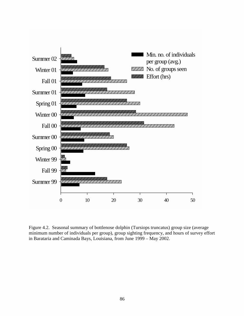
86
0 10 20 30 40 50
Summer 99
Fall 99
Winter 99
Spring 00
Summer 00
Fall 00
Winter 00
Spring 01
Summer 01
Fall 01
Winter 01
Summer 02Min. no. of individualsper group (avg.)No. of groups seenEffort (hrs)
Figure 4.2. Seasonal summary of bottlenose dolphin (Tursiops truncatus) group size (average minimum number of individuals per group), group sighting frequency, and hours of survey effort in Barataria and Caminada Bays, Louisiana, from June 1999 – May 2002.
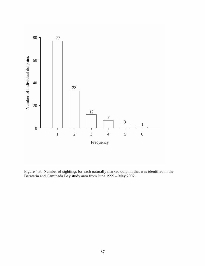
87
Frequency
1 2 3 4 5 6
Num
ber o
f ind
ivid
ual d
olph
ins
0
20
40
60
80 77
33
127
31
Figure 4.3. Number of sightings for each naturally marked dolphin that was identified in the Barataria and Caminada Bay study area from June 1999 – May 2002.
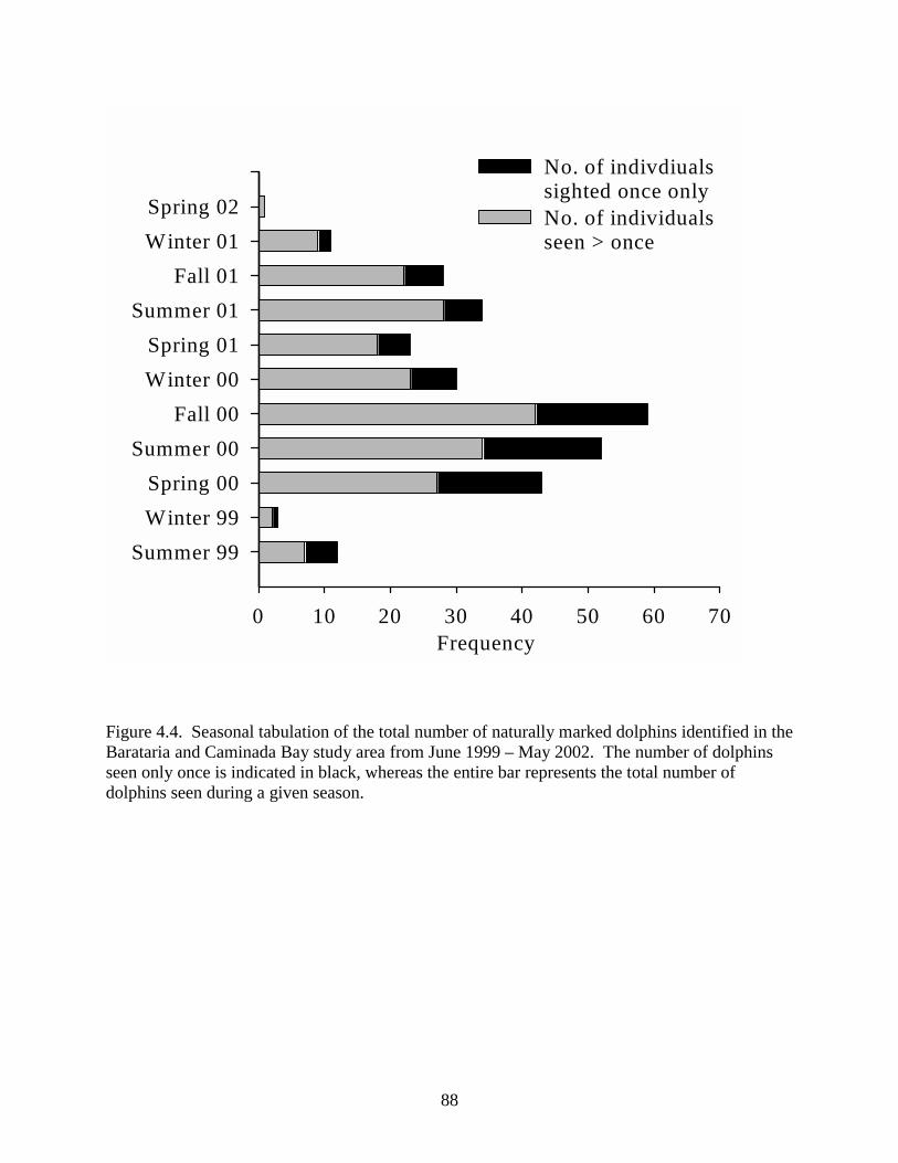
88
Frequency0 10 20 30 40 50 60 70
Summer 99Winter 99Spring 00
Summer 00Fall 00
Winter 00Spring 01
Summer 01Fall 01
Winter 01Spring 02
No. of indivdiuals sighted once onlyNo. of individualsseen > once
Figure 4.4. Seasonal tabulation of the total number of naturally marked dolphins identified in the Barataria and Caminada Bay study area from June 1999 – May 2002. The number of dolphins seen only once is indicated in black, whereas the entire bar represents the total number of dolphins seen during a given season.
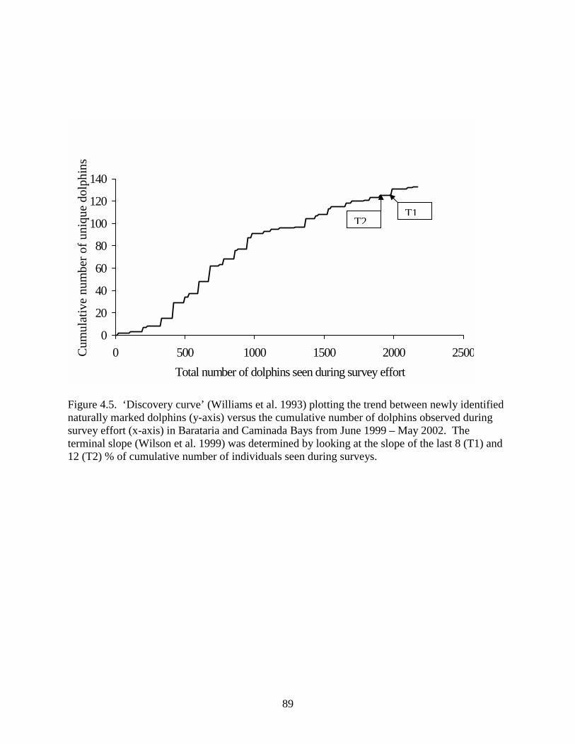
89
Total number of dolphins seen during survey effort0 500 1000 1500 2000 2500C
umul
ativ
e nu
mbe
r of u
niqu
e do
lphi
ns
0
20
40
60
80
100
120
140
Figure 4.5. ‘Discovery curve’ (Williams et al. 1993) plotting the trend between newly identified naturally marked dolphins (y-axis) versus the cumulative number of dolphins observed during survey effort (x-axis) in Barataria and Caminada Bays from June 1999 – May 2002. The terminal slope (Wilson et al. 1999) was determined by looking at the slope of the last 8 (T1) and 12 (T2) % of cumulative number of individuals seen during surveys.
T1T2
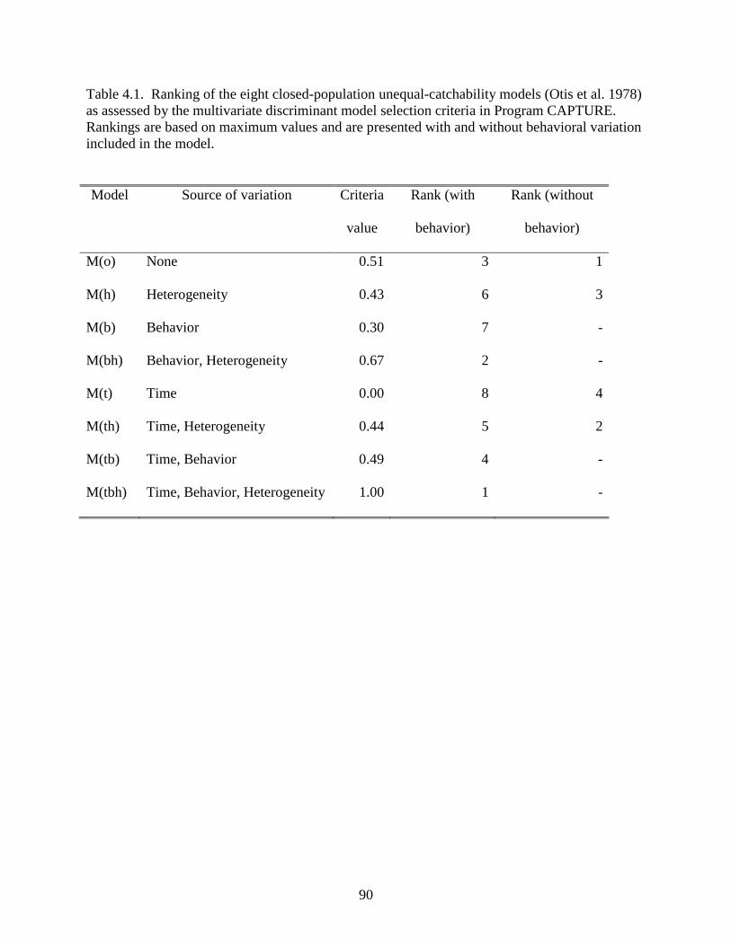
90
Table 4.1. Ranking of the eight closed-population unequal-catchability models (Otis et al. 1978) as assessed by the multivariate discriminant model selection criteria in Program CAPTURE. Rankings are based on maximum values and are presented with and without behavioral variation included in the model.
Model Source of variation Criteria
value
Rank (with
behavior)
Rank (without
behavior)
M(o) None 0.51 3 1
M(h) Heterogeneity 0.43 6 3
M(b) Behavior 0.30 7 -
M(bh) Behavior, Heterogeneity 0.67 2 -
M(t) Time 0.00 8 4
M(th) Time, Heterogeneity 0.44 5 2
M(tb) Time, Behavior 0.49 4 -
M(tbh) Time, Behavior, Heterogeneity 1.00 1 -
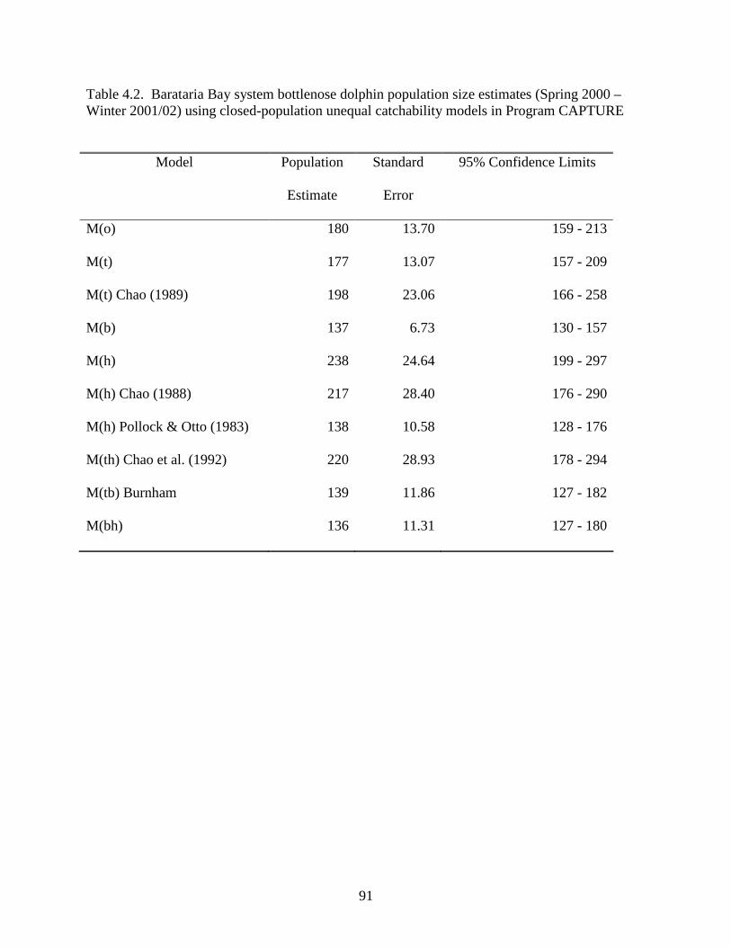
91
Table 4.2. Barataria Bay system bottlenose dolphin population size estimates (Spring 2000 – Winter 2001/02) using closed-population unequal catchability models in Program CAPTURE
Model Population
Estimate
Standard
Error
95% Confidence Limits
M(o) 180 13.70 159 - 213
M(t) 177 13.07 157 - 209
M(t) Chao (1989) 198 23.06 166 - 258
M(b) 137 6.73 130 - 157
M(h) 238 24.64 199 - 297
M(h) Chao (1988) 217 28.40 176 - 290
M(h) Pollock & Otto (1983) 138 10.58 128 - 176
M(th) Chao et al. (1992) 220 28.93 178 - 294
M(tb) Burnham 139 11.86 127 - 182
M(bh) 136 11.31 127 - 180
92
was: M(o), M(th), M(h) and M(t). Model selection criteria for all four models were below the
suggested cut-off score of 0.75; however, since these models are a subset of all eight models this
may be a moot point. Chi-square goodness-of-fit tests found that models including time and
heterogeneity fit the data significantly better (α < 0.001) than the more general model M(o).
Hence, the variability in sighting probabilities is difficult to conclusively explain. All four
models produced fairly similar population estimates; 138 – 238 with an associated 95% CL range
of 128 – 297. The only two models whose 95% CLs did not overlap with each other were the
Pollock and Otto estimator for M(h) (95% CL = 128-176) and the Chao estimator for M(th)
(95% CL = 178-294).
MARK was used to model sighting rates on a yearly, seasonal (with data combined
across years), and seasonal (with data separated between years) scales. In addition a constant
rate of sighting was also investigated (Tables 4.3 – 4.7). Likelihood-ratio tests showed that
seasonal (data not combined across years) variability described the data significantly better than
any other configuration of temporal variance (Table 4.3). It should also be apparent that Models
A and D (Table 4.3) are identical to CAPTURE models M(t) and M(o), respectively (Table 4.2).
When temporal variability was broken down further into monthly time intervals, the resulting
models became over-parameterized and produced singular estimates.
DISCUSSION
The first photo-identification research effort for a bottlenose dolphin population in
Louisiana’s Barataria Basin system offered several important conclusions and findings. First,
with regard to population size, this recent and year-round survey effort of bottlenose dolphins in
Barataria and Caminada bays has produced an abundance estimate of between 138 and 238
individuals for this region. The population appears to be relatively closed with some evidence of
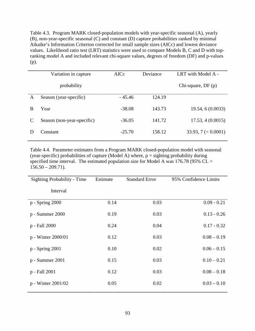
93
Table 4.3. Program MARK closed-population models with year-specific seasonal (A), yearly (B), non-year-specific seasonal (C) and constant (D) capture probabilities ranked by minimal Aikaike’s Information Criterion corrected for small sample sizes (AICc) and lowest deviance values. Likelihood ratio test (LRT) statistics were used to compare Models B, C and D with top-ranking model A and included relevant chi-square values, degrees of freedom (DF) and p-values (p).
Variation in capture
probability
AICc Deviance LRT with Model A -
Chi-square, DF (p)
A Season (year-specific) - 45.46 124.19
B Year -38.08 143.73 19.54, 6 (0.0033)
C Season (non-year-specific) -36.05 141.72 17.53, 4 (0.0015)
D Constant -25.70 158.12 33.93, 7 (< 0.0001)
Table 4.4. Parameter estimates from a Program MARK closed-population model with seasonal (year-specific) probabilities of capture (Model A) where, p = sighting probability during specified time interval. The estimated population size for Model A was 176.78 (95% CL = 156.50 – 209.71). Sighting Probability - Time
Interval
Estimate Standard Error 95% Confidence Limits
p - Spring 2000 0.14 0.03 0.09 - 0.21
p - Summer 2000 0.19 0.03 0.13 - 0.26
p - Fall 2000 0.24 0.04 0.17 - 0.32
p - Winter 2000/01 0.12 0.03 0.08 – 0.19
p - Spring 2001 0.10 0.02 0.06 – 0.15
p - Summer 2001 0.15 0.03 0.10 – 0.21
p - Fall 2001 0.12 0.03 0.08 – 0.18
p - Winter 2001/02 0.05 0.02 0.03 – 0.10
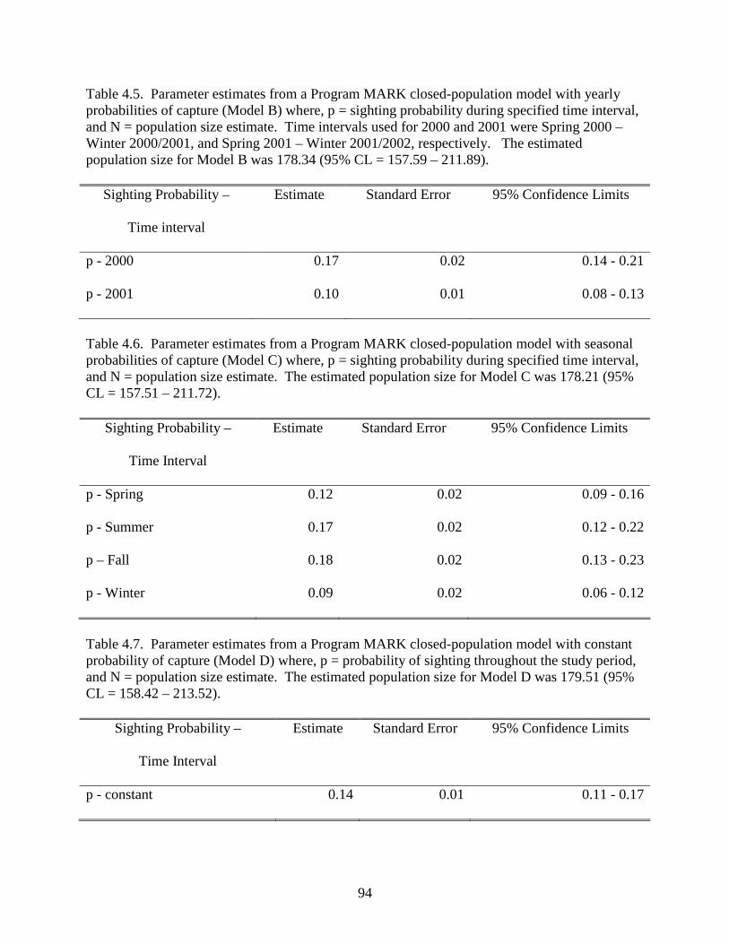
94
Table 4.5. Parameter estimates from a Program MARK closed-population model with yearly probabilities of capture (Model B) where, p = sighting probability during specified time interval, and N = population size estimate. Time intervals used for 2000 and 2001 were Spring 2000 – Winter 2000/2001, and Spring 2001 – Winter 2001/2002, respectively. The estimated population size for Model B was 178.34 (95% CL = 157.59 – 211.89).
Sighting Probability –
Time interval
Estimate Standard Error 95% Confidence Limits
p - 2000 0.17 0.02 0.14 - 0.21
p - 2001 0.10 0.01 0.08 - 0.13
Table 4.6. Parameter estimates from a Program MARK closed-population model with seasonal probabilities of capture (Model C) where, p = sighting probability during specified time interval, and N = population size estimate. The estimated population size for Model C was 178.21 (95% CL = 157.51 – 211.72).
Sighting Probability –
Time Interval
Estimate Standard Error 95% Confidence Limits
p - Spring 0.12 0.02 0.09 - 0.16
p - Summer 0.17 0.02 0.12 - 0.22
p – Fall 0.18 0.02 0.13 - 0.23
p - Winter 0.09 0.02 0.06 - 0.12
Table 4.7. Parameter estimates from a Program MARK closed-population model with constant probability of capture (Model D) where, p = probability of sighting throughout the study period, and N = population size estimate. The estimated population size for Model D was 179.51 (95% CL = 158.42 – 213.52).
Sighting Probability –
Time Interval
Estimate Standard Error 95% Confidence Limits
p - constant 0.14 0.01 0.11 - 0.17
95
site fidelity. Furthermore, the documentation and identification of individual dolphins allows the
possibility of comparisons with future studies both in the study area and with those catalogued in
other areas of the Gulf of Mexico. Secondly, with regard to variability in sighting probability
both programs CAPTURE and MARK strongly indicated that sighting histories of bottlenose
dolphins present in the Barataria Basin were variable over time and between individuals.
However, determination of whether this variation in sighting probability was specifically
attributable to temporal factors (such as season), differences in probability of capture for
individuals, or a combination of these factors could not be resolved definitively.
Population Size
Barataria Bay has been recognized as a distinct stock by the U.S. Atlantic and Gulf of
Mexico marine mammal stock assessments (Waring et al. 2002). Directly seaward of this
purported stock is the western Gulf of Mexico (wGOM) coastal bottlenose dolphin stock. The
wGOM stock is characterized as inhabiting the near-shore coastal waters (i.e., from the coastline
or presumed bay boundary to 9.3 km seaward of the 18.3 m isobath) from the Texas border to the
Mississippi River mouth. Separation of Barataria Bay and wGOM coastal stocks is based on
evidence of genetic differentiation between offshore and inshore stocks in other regions
(Duffield and Wells 1986) as well as the assumption that the unique oceanographic regimes of
inshore and offshore waters would limit movement. The proximity of the Barataria Bay and
wGOM stocks makes these distinctions difficult to confirm. However, the meaning of a
management stock in this context is not synonymous with the traditional biological definition of
a population (Pollock et al. 1990). The term is based on the description of a “community” (after
Wells et al. 1987) in which dolphins have a high site-fidelity to the given area (so-called
“residents”), possess similar genetic profiles, and interact primarily with each other. This
96
definition permits the possibility of interbreeding with outside members as well as movement
into and out of the stock management area. Although a majority of the designated estuarine
stocks within the Gulf of Mexico may not strictly fall within the definition of a biological
population, they can be described as functioning units of their ecosystem and so are correctly
considered discrete under the Marine Mammal Protection Act. The 2002 U.S. Atlantic and Gulf
of Mexico Marine Mammal Stock Assessments (Waring et al. 2002) suggests that “biologically-
based” criteria, such as movement patterns, genetic profiling and contaminant loads, be
combined with traditional field observations to define stock memberships.
High site fidelity has been noted in some coastal estuarine areas of the Gulf of Mexico
(Scott et al. 1990, Wells 1991) but not all (Hubard 1998, Maze and Wursig 1999). All
population models used in my results were closed-population models. My preliminary surveys
of the region ascertained the geographic extent of this population. However, it is unlikely that
the closure assumption was strictly met, as evidenced by the high number of individuals sighted
only once and the low incidence of re-sightings. Alternatively, the discovery curve indicated a
steady decrease in the number of new individuals seen as effort accumulated. The terminal rate
of discovery suggests that the Barataria Basin population was relatively closed (Figure 4.5). The
range of terminal slopes for this study (0.001 – 0.01) is comparable to Wilson et al.’s (1999) rate
of 0.012 for sub-adults and 0.011 for adults in a closed bottlenose dolphin population in Moray
Firth, Scotland. However, as noted in Figure 4.3, a majority (77 out of 133 = 58%) of
individuals were seen in Barataria Basin on only one occasion. Additionally, my findings are
weakened by the fact that this project was a new initiative and survey effort was limited.
Furthermore, the detection of significant variability in both temporal and individual sighting
rates makes my assumption of population closure provisional.
97
Extending the duration and geographical extent of the present study is required to
strengthen my findings. Proximity to the Western Gulf of Mexico coastal stock as well as the
estuarine stock of the Terrebonne and Timbalier bay complex makes interchange with each of
these purported populations a plausible occurrence. However, whether these possible
interactions are in accord with the flexible Wells et al. (1987) population definition and therefore
mirror the social structure of western Florida estuarine stocks, or suggest that the Barataria bay
stock is in fact part of a larger northern Gulf of Mexico meta-population requires further
investigation.
Variability in Sighting Probability
There are many reasons why individuals have unique probabilities of being sighted
during observation periods (Hammond 1990). Individual attributes such as age, gender, social
status, and stock association are possible factors influencing both distribution and behavior
patterns. Environmental conditions such as movement of potential prey, proximity to fishing
vessels, and oceanographic features may also influence sighting probability on a given survey. It
is also important to consider possible bias introduced by such avenues as data acquisition,
verification of image matching and distinction, and modeling strategy.
Survey strategy can also cause some additional heterogeneity in capture. Non-random
mixing of individuals may allow some animals to be seen more often. Moreover, surveys that
are not randomized or comprehensive in their coverage of a population’s range will also
introduce heterogeneity. In these surveys I attempted to minimize heterogeneity by introducing a
stratified survey design to ensure that no regions of the study area were preferentially covered or
confounded with time of day. Results from model outputs indicated that temporal variability
was significant. The occurrence and relative frequency of individuals sighted appeared to be
98
different between 2000 and 2001 (Figures 4.2 and 4.4), yet this configuration (i.e., yearly
variation in capture only) was not the best fit for the data according to MARK (Table 4.3). A
closer look at the data revealed that these differences appeared to be driven by the small numbers
of recaptures in Spring 2001 and Winter 2001/2002. Effort during both of these seasons was
comparable to other months, though number of groups seen in Winter 2001/2002 did appear to
be slightly lower (Figure 4.2). Logbook entries made during Winter 2001/2002 also indicated
that climatic conditions were not ideal for taking photographs. However, survey routes during
both seasons were random, covered the study area well, and had experienced observers aboard at
all times. It may be possible that unknown behavioral processes, a unique age structuring of the
population, or activities in the area may have been the cause of these anomalies in number of re-
sightings.
Sources of variability in capture may mask each other to produce ambiguity in
interpretation of model results (Otis et al. 1978). Although some of the tests in CAPTURE lack
power, null hypotheses were being rejected and so the conclusions are most likely accurate.
Relative effort and number of re-sightings can also affect model results. Precision is positively
correlated with increasing capture probability (Cormack 1968). In my Program MARK results
(Tables 4.4 – 4.7) capture probabilities ranged from 0.05 to 0.24 with a mean of approximately
0.14, and fell between the medium (mean ≈ 0.20) to poor (mean ≈ 0.05) classifications of data.
Using simulated data, Otis et al. (1978) found medium quality data to correctly select the models
M(o), M(th), M(h) and M(t) with the following percentages: 68.0, 25.5, 66.5 and 57.5. For poor
data these percentages changed to 79.0, 5.0, 18.5 and 83.5, respectively. It should be noted that
selection of the incorrect model for the simulated data did not always results in estimates that
were significantly different from the true population size.
99
In addition to the assumptions of population closure and equal catchability, the
population models used in this study also require that marks are not lost and that marks are
correctly identified. Therefore, the natural marking used on individuals must be permanent and
sufficiently distinct for the duration of the study, and the images used for each individual must be
of sufficient quality to allow consistent identification. Lockyer and Morris (1990) found
superficial and deeper scratches, as well as minor wounds to be inadequate natural markings on
bottlenose dolphins. They also found that the head, back, dorsal fin and tail flukes were the most
likely areas for permanent markings. Wursig and Wursig (1977) noted that both pigment spots
and bite marks did not remain visible throughout their study of bottlenose dolphins in Argentina.
I found dorsal fin nicks and notches to be suitable and effective natural markings for my study.
However, as Hammond (1986) cautions it is important to note that evidence of persistence of a
given type of mark does not guarantee identical results from similar wounds. The loss of natural
markings would cause population estimates to be inflated.
Treatment of processed images is the next step in ensuring that bias does not enter an
abundance assessment. It is imperative that the quality of images used is consistently excellent.
Image quality classification must be made independently of the presence or extent of natural
markings present on the individual (Friday et al. 2000). This independence ensures that the most
distinctive individuals will not be preferentially included or matched. For accurate population
estimates it is also important that non-preferential picture acquisition is practiced. Finally,
matching efficiency of bottlenose dolphin natural fin markings has greatly benefited by the
description of the dorsal fin ratio methods by Defran et al. (1990), as well as the Finscan
software developed by Kreho et al. (1999), to assist and speed up a related process.
100
CONCLUSIONS
Both similarities and differences in residency patterns of individual bottlenose dolphins
present in Barataria and Caminada bays, as compared with other regions of the Gulf of Mexico
contribute to the understanding of population dynamics for this region. Valuable insight into the
life history patterns of bottlenose dolphin populations can also be achieved by investigating
population models that are able to account for differences in sighting rates. Significant
variability in probability of sighting was found on both temporal and individual scales.
However, several other confounding sources affecting the behavior and distribution patterns of
wild bottlenose dolphin populations require consideration also (Hammond et al. 1990). Social
stability and associations have been well established in cetacean populations (Bigg et al. 1990,
Wells 1991). The inherent lack of independence between social affiliates violates assumptions
of many basic closed-population models. Although this matter requires further investigation, it
potentially affects precision but not necessarily the accuracy of estimators (Wilson et al. 1999).
Another factor worthy of consideration is the role that type of activity and group size play in the
ability to detect a given individual or group. For example, it seems logical that larger groups or
highly acrobatic behaviors would be more visible during surveys. Likewise, one or two
individuals engaged in activities with relatively long dive times would be correspondingly more
difficult to detect. Some detectability models have been developed (Steinhorst and Samuel
1989) but are not widely incorporated in marine mammal research currently. Additional
concerns such as the presence of boat traffic, fishing vessels, and recreational activities in the
area all figure into the ability to detect and sample individual dolphins. The use of unequal-
catchability models is a starting point for assessing some of these factors, yet it is far from a
comprehensive solution. An appropriate future direction is to investigate models that are able to
101
include some of the above-mentioned covariates, such as Forney et al. (1991) was able to do with
sea-state in a model for harbor porpoise. Furthermore, the delineation of behavioral or
demographic strata of the population with specific sighting rates should also act to increase the
relative precision of resulting estimates. In short, any quantitative or qualitative variable that is
able to help identify patterns of cetacean distribution is a useful tool for better understanding
marine mammal populations and improving the precision and accuracy of population
assessments.
LITERATURE CITED Akaike, H. 1973. Information theory as an extension of the maximum likelihood principle. Pages 267-281 in B. N. Petrov and F. Csaki, eds. Second International Symposium on Information Theory. Akademiai Kiado, Budapest. Allen, M. C. and A. Read. 2000. Habitat selection of foraging bottlenose dolphins in relation to boat density near Clearwater, Florida. Marine Mammal Science 16:815-824. Baird, R. W. and P. J. Stacey. 1988. Variation in saddle patch pigmentation in populations of killer whales (Orcinus orca) from British Columbia, Alaska, and Washington state. Canadian Journal of Zoology 66:2582-2585. Bannister, J. L. 1990. Southern right whales off Western Australia. Report of the International Whaling Commission (Special Issue) 12: 279-288. Bigg, M. A., P. F. Olesiuk, G. M. Ellis, J. K. B. Ford and K. C. Balcomb III. 1990. Social organization and genealogy of resident killer whales (Orcinus orca) in the coastal waters of British Columbia and Washington State. Report of the International Whaling Commission (Special Issue) 12: 383-405. Blaylock, R. A. and W. Hoggard. 1994. Preliminary estimates of bottlenose dolphin abundance in southern U.S. Atlantic and Gulf of Mexico continental shelf water. NOAA Technical Memorandum. NMFS-SEFSC-356, 10pp. Cerchio, S. 1998. Estimates of humpback whale abundance off Kauai, 1989 to 1993: evaluating biases associated with sampling the Hawaiian Islands breeding assemblage. Marine Ecology Progress Series 175:23-34. Cerchio, S., C. M. Gabriele, T. F. Norris and L. M. Herman. 1998. Movements of humpback whales between Kauai and Hawaii: implications for population structure and abundance estimation in the Hawaiian Islands. Marine Ecology Progress Series 175:13-22.
102
Chao, A. 1988. Estimating animal abundance with capture frequency data. Journal of Wildlife Management 52:295-300. Chao, A. 1989. Estimating population size for sparse data in capture-recapture experiments. Biometrics 45:427-438. Chao, A. 2001. An overview of closed capture-recapture models. Journal of Agricultural, Biological and Environmental Statistics 6:158-175. Connor, W. H. and J. W. Day, Jr. 1987. The ecology of Barataria Basin, Louisiana: an estuarine profile. U.S. Fish and Wildlife Service Biological Report 85 (7.13). 165 pp. Cormack, R. M. 1968. The statistics of capture-recapture methods. Oceanography and Marine Biology - An Annual Review 6:455-506. Defran, R. H., G. M. Shultz and D. W. Weller. 1990. A technique for the photographic identification and cataloging of dorsal fins of the bottlenose dolphin (Tursiops truncatus). Report of the International Whaling Commission (Special Issue) 12:53-55. Duffield, D. A. and R. S. Wells. 1986. Population structure of bottlenose dolphins: Genetic studies of bottlenose dolphins along the central west coast of Florida. Contract Report to National Marine Fisheries Serivce, Southeast Fisheries Center, contract No. 45-WCNF-5- 00366, 16 pp. Forney, K. A., D. A. Hanan and J. Barlow. 1991. Detecting trends in harbor porpoise abundance from aerial surveys using analysis of covariance. Fishery Bulletin 89: 367- 377. Friday, N., T. D. Smith, P. T. Stevick and J. Allen. 2000. Measurement of photographic quality and individual distinctiveness for the photographic identification of humpback whales, Megaptera novaeangliae. Marine Mammal Science 116: 355-374. Fritts, T. H., A. B. Irvine, R. D. Jennings, L. A. Collum, W. Hoffman and M. A. McGehee. 1983. Turtles, birds and mammals in the northern Gulf of Mexico and nearby Atlantic waters. U.S. Fish and Wildlife Service, Washington D.C. FWS/OBS-82165. 455pp. Hammond, P. S. 1986. Estimating the size of naturally marked whale populations using capture-recapture techniques. Report of the International Whaling Commission (Special Issue) 8: 253-282. Hammond, P. S. 1990. Heterogeneity in the Gulf of Maine? Estimating humpback whale population size when capture probabilities are not equal. Report of the International Whaling Commission (Special Issue) 12: 135-139.
103
Hammond, P. S., S. A. Mizroch, and G. P. Donovan, Eds. 1990. Individual recognition of cetaceans: use of photo-identification and other techniques to estimate population parameters. Report of the International Whaling Commission (Special Issue) 12. Hubard, C. W. 1998. Abundance, distribution, and site fidelity of bottlenose dolphins in Mississippi Sound, Mississippi. M.S. thesis, University of Alabama, Tuscaloosca, Alabama, 101 p. Hurvich, C. M., and C-L. Tsai. 1989. Regression and time series model selection in small samples. Biometrika 76: 297-307. Jefferson, T. A. 1996. Estimates of abundance of cetaceans in offshore waters of the northwestern Gulf of Mexico, 1992-1993. The Southwestern Naturalist 41: 279-287. Kreho, A., N. Kehtarnavaz, B. Araabi, G. Hillman, B. Wursig and D. Weller. 1999. Assisting manual dolphin identification by computer extraction of dorsal ratio. Annals of Biomedical Engineering 27:830-838. Lincoln, F. C. 1930. Calculating waterfowl abundance on the basis of banding returns. United States Department of Agriculture Circular 118: 1-4. Lockyer, C. H. and R. J. Morris. 1990. Some observations on wound healing and persistence of scars in Tursiops truncatus. Report of the International Whaling Commission (Special Issue) 12:113-118. Maze, K. S., and B. Wursig. 1999. Bottlenose dolphins of San Luis Pass, Texas: Occurrence patterns, site-fidelity, and habitat use. Aquatic Mammals 25:91-103. Mullin, K. D. 1988. Comparative seasonal abundance and ecology of bottlenose dolphins (Tursiops truncatus) in three habitats of the north-central Gulf of Mexico. Ph.D. dissertation, Mississippi State University 135 p. Mullin, K. D., R. R. Lohoefener, W. Hoggard, C. L. Roden and C. M. Rogers. 1990. Abundance of bottlenose dolphins, Tursiops truncatus, in the coastal Gulf of Mexico. Northeast Gulf Science 11: 113-122. Mullin, K. D., W. Hoggard, C. L. Roden, R. R. Lohefener, C. M. Rogers and B. Taggart. 1994. Cetaceans on the upper continental slope in the north-central Gulf of Mexico. Fishery Bulletin 92: 773-786. Olesiuk, P. F., M. A. Bigg and G. M. Ellis. 1990. Life history and population dynamics of resident killer whales (Orcinus orca) in the coastal waters of British Columbia and Washington state. Report of the International Whaling Commission (Special Issue) 12: 209-243. Otis, D. L., K. P. Burnham, G. C. White and D. R. Anderson. 1978. Statistical Inference from Capture data on closed animal populations. Wildlife Monographs 62:1-135.
104
Payne, R., V. Rowntree and J. S. Perkins. 1990. Population size, trends and reproductive parameters of right whales (Eubalaena australis) off Peninsula Valdes, Argentina. Report of the International Whaling Commission (Special Issue) 12: 271-278. Petersen, C. G. T. 1896. The yearly immigration of young plaice into the Limfjord from the German Sea. Report of Danish Biological Station 6: 1-48. Pollock, K. H. and M. C. Otto. 1983. Robust estimation of population size in closed animal population from capture-recapture experiments. Biometrics 39:1035-1049. Pollock, K. H., J. D. Nichols, C. Brownie and J. E. Hines. 1990. Statistical Inference for Capture-recapture experiments. Wildlife Monographs 107: 1-97. Reed, D., ed. 1995. Status and trends of hydrologic modification, reduction in sediment availablity and habitat loss/modification in the Barataria-Terrebonne estuarine system. Barataria-Terrebonne National Estuary Program (Publication #20). 338pp. Available from Barataria-Terrebonne National Estuary Program Office, Nicholls State University Campus, P.O. Box 2663, Thibodaux, LA 70310. Rexstad, E., and K. Burnham. 1991. User’s guide to interactive program CAPTURE. Colorado Cooperative Fish and Wildlife Research Unit, Colorado State University, Fort Collins, Colorado 80523 U.S.A. Scott, G. P., D. M. Burn, L. J. Hansen and R. E. Owen. 1989. Estimates of bottlenose abundance in the Gulf of Mexico from regional aerial surveys. CRD 88/89-07. Scott, G. P., R. S. Wells, and A. B. Irvine. 1990. A long-term study of bottlenose dolphins on the west coast of Florida. Pages 235-244 in S. Leatherwood and R. R. Reeves, eds. The bottlenose dolphin. Academic Press, San Diego, California. Steinhorst, R. K. and M. D. Samuel. 1989. Sightability adjustment methods for aerial surveys of wildlife populations. Biometrics 45: 415-425. Urian, K. W. and R. S. Wells. 1996. Bottlenose dolphin photo-identification workshop: March 21-22, 1996, Charleston, South Carolina. NOAA Technical Memorandum NMFS- SEFSC-393. Waring, G.T., J.M. Quintal and C.P. Fairfield, eds. 2002. U.S. Atlantic and Gulf of Mexico marine mammal stock assessments. NOAA Technical Memorandum NMFS-NE-169. vii + 180 + 4 app. Wells, R. 1991. The role of long-term study in understanding the social structure of a bottlenose dolphin community. Pages 199-225 in K. Pryor and K. S. Norris, eds. Dolphin societies: Discoveries and Puzzles. University of California, Santa Cruz, California.
105
Wells, R. S., M. D. Scott and A. B. Irvine. 1987. The social structure of free-ranging bottlenose dolphins. Pages 247-305 in H. Genoways, ed. Current Mammalogy, Vol. 1. Plenum Press, New York, New York. White, G.C. and K. P. Burnham. 1999. Program MARK: Survival estimation from populations of marked animals. Bird Study (supplement) 46:120-138. Whitehead, H. 1990. Mark-recapture estimates with emigration and re-immigration. Biometrics 46:473-479. Whitehead, H. and S. Waters. 1990. Social organization and population structure of sperm whales off the Galapagos Islands, Ecuador (1985 and 1987). Report of the International Whaling Commission (Special Issue) 12: 249-257. Williams, J. A., S. M. Dawson, and E. Slooten. 1993. The abundance and distribution of bottlenose dolphins Tursiops truncatus in Doubtful Sound, New Zealand. Canadian Journal of Zoology 71:2080-2088. Wilson, B., P. S. Hammond and P. M. Thompson. 1999. Estimating size and assessing trends in a coastal bottlenose dolphin population. Ecological Applications 9:288-300.
Wursig, B., F. Cipriano and M. Wursig. 1991. Dolphin movement patterns: Information from radio and theodolite tracking studies. Pages 79-112 in K. Pryor and K. S. Norris, eds. Dolphin societies: Discoveries and Puzzles. University of California, Santa Cruz, California.
Wursig, B and M. Wursig. 1977. The photographic determination of group size, composition, and stability of coastal porpoises (Tursiops truncatus). Science 198: 755-756.
106
CHAPTER V
DISCUSSION
The bottlenose dolphin (Tursiops truncatus) is a well-studied member of the Order
Cetacea (Shane et al. 1986, Leatherwood and Reeves 1990) and has been observed in a wide
variety of habitats worldwide (Connor and Smolker 1985, Cockroft et al. 1990, Ballance 1992,
Williams et al. 1993, Grigg and Markowitz 1997, Harzen 1998, Wilson et al. 1999). Although
several projects have focused on bottlenose dolphin populations and “communities” (see Wells et
al. 1987) within the northern Gulf of Mexico (Shane 1980, Wells et al. 1987, Mullin 1988, Scott
et al. 1990, Wells and Scott 1990, Wells 1991, Brager 1993, Hubard 1998, Maze and Wursig
1999), there has been limited research effort along the Louisiana coast (Hubard and Swartz 2002,
Waring et al. 2002). This study focused on the ecology of bottlenose dolphins in lower Barataria
and Caminada bays, Louisiana, by combining fine-scale measurements of habitat use and
individual identification techniques to describe environmental requirements (Chapter II) and
estimate population size (Chapter IV). The latter portion of the field research was further
investigated by examining assumptions of the Jolly-Seber model when used to estimate
population size of cetaceans from photo-identification data (Chapter III). This research is
important because dynamic changes in the Louisiana coastal zone place unknown stressors on
the poorly studied bottlenose dolphins in this area. However, trends in abundance can only be
determined when satisfactory survey methodology and analyses are used to estimate population
size from recent survey effort.
There are several factors that make the Barataria Bay system an interesting location for
small cetacean research. Barataria and Caminada bays represent the seaward interface of the
Barataria Basin with the northern Gulf of Mexico (Reed 1995). The low-lying inland wetlands
107
include marsh grasses, submerged aquatic vegetation and estuarine ponds (Chesney et al. 2000).
Estuarine areas are known to provide important nursery habitat to fishes and crustaceans (Baltz
et al. 1998) and have high primary productivity rates (Day et al. 1989, Garrison 1999).
However, the Louisiana coastline has undergone significant changes in recent years (Day et al.
1995, Turner 1997). In fact, coastal wetland losses from 1955 to 1978 are estimated to have
been as high as 12,700 ha per annum (Baumann and Turner 1990). The continued modification
of habitat may have serious repercussions for numerous species in coastal Louisiana ecosystems
(Chesney et al. 2000), including bottlenose dolphins.
The description of bottlenose dolphin environmental usage patterns of the Barataria Basin
system developed by this study strengthens the database for appropriate management of this
relatively discrete Gulf of Mexico stock. Firstly, the unique and changing environment makes it
especially important to develop a defendable baseline study of present bottlenose dolphin
population size so that any trends associated with habitat loss may be detected. Secondly, the
characterization of environmental requirements is valuable because dissimilar oceanographic
conditions are cited as one reason for the existence of distinctive inshore and offshore bottlenose
dolphin stocks in coastal Louisiana and elsewhere in the northern Gulf of Mexico (Duffield et al.
1983, Duffield and Wells 1986, Waring et al. 2002). Therefore, the careful description of the
habitat use by an inshore stock may allow specific differences with the environment of offshore
stocks to be detected. It should be noted that environmental habitat usage patterns described in
this study characterized habitat selection of measured variables at sites where individuals were
observed, but not where they were absent. The basic advantage of this approach is that it uses
the bottlenose dolphin’s behavior to describe its distribution and abundance in the system and
creates a description of environmental requirements from a dolphin’s point-of-view (Baltz 1990,
108
Chesney et al. 2000). Future research that is able to accurately characterize the entire study area
could provide insights into habitat usage for general and specific activities. I addressed this in a
limited fashion using suitability analyses (Chapter II) to compare general habitat use and feeding
site selection, but a better characterization of resource availability would greatly increase our
understanding of bottlenose dolphin ecology in the Barataria Basin. Likewise, the inclusion of
additional environmental variables (such as water velocity, density of boat traffic and presence of
prey) as related to patterns of habitat use would clearly enhance insights into possible
interactions within the Barataria Basin ecosystem.
Using closed-population unequal-catchability models (Otis et al. 1978) I estimated that
138 – 238 (with associate range of 95% Confidence Limits = 128 – 297) (Chapter IV) bottlenose
dolphins were present in my study area. While this is an important contribution to knowledge of
bottlenose dolphins in this area, continued year-round monitoring of this population is necessary
to detect possible declines and seasonal fluctuations in abundance levels. A methodology for
assessing the status of U.S. marine mammal stocks was developed by Wade and Angliss (1997)
with limits of mortality being determined by calculation of the potential biological removal
(PBR) for the given population (Wade 1997). The PBR is a fisher-related mortality limit which
is derived from the product of the minimum population size (i.e., the lower 20th percentile of the
distribution of the abundance estimate), maximum population growth rate of the population, and
a “recovery factor” based on relative status of the population relative to optimum sustainable
population (OSP) (Waring et al. 2002). The current PBR of 1.4 individuals for the Barataria Bay
stock (Waring et al. 2002) is based on a population size of 219 individuals as estimated by aerial
surveys conducted over a decade ago (Blaylock and Hoggard 1994). This population estimate
falls well within the range of estimates produced from my dissertation research. However, if the

109
lower end of my estimates accurately reflects current population levels, the management strategy
is misjudging the influence that fishery-related mortalities place on this population and PBR
levels should be lowered.
The determination of population closure for the Barataria system was based on
decreasing numbers of previously unseen marked individuals as survey effort accumulated, as
well as evidence of some degree of site-fidelity for numerous individuals. However, clarification
of this tentative characterization as a closed population would obviously benefit from continued
research efforts in and adjacent to the study area. As noted in my examination of Jolly-Seber
model assumptions (Chapter III) it is imperative that any samples taken be representative of the
true population in order for accurate and precise estimates to be made. Extending the duration,
intensity and coverage of this initial photo-identification study is an obvious and necessary first
step toward satisfying this requirement. Specifically, the geographic range, temporal variation in
abundance, and site-fidelity of uniquely identified individuals could be confirmed and more
definitively understood. For example, performing similar surveys in regions overlapping the
southern end of my study area and extending out onto the central Louisiana coast would be one
way to address pertinent stock structure questions.
Findings from this research provide an innovative approach to describing environmental
habitat use for dolphins, highlight the necessity to assess statistical methodology when
estimating population size from cetacean photo-identification data, and aid in filling important
gaps in the understanding of northern Gulf of Mexico bottlenose dolphin stock structure and
population dynamics (Hubard and Swartz 2002).
LITERATURE CITED Ballance, L. 1992. Habitat use patterns and ranges of the bottlenose dolphin in the Gulf of California, Mexico. Marine Mammal Science 8:262-274.
110
Baltz, D. M. 1990. Chapter 18, Autecology. Pages 585-607 in Methods for Fish Biology. C. B. Shreck and P. B. Moyle (eds.). American Fisheries Society. Bethesda, Maryland. Baltz, D. B., J. W. Fleeger, C. F. Rakocinski and J. N. McCall. 1998. Food, density, and microhabitat: factors affecting growth and recruitment potential of juvenile saltmarsh fishes. Environmental Biology of Fishes 53:89-103. Baumann, R. H. and R. E. Turner. 1990. Direct impact of the outer continental shelf activities on wetland loss in the central Gulf of Mexico. Environmental Geology and Water Resources 15:189-198. Blaylock, R. A. and W. Hoggard. 1994. Preliminary estimates of bottlenose dolphin abundance in southern U.S. Atlantic and Gulf of Mexico continental shelf waters. NOAA Technical Memorandum. NMFS-SEFSC-356, 10 pp. Brager, S. 1993. Diurnal and seasonal behavior patterns of bottlenose dolphins (Tursiops truncatus). Marine Mammal Science 9:434-440. Chesney, E. J., D. M. Baltz and R. G. Thomas. 2000. Louisiana estuarine and coastal fisheries and habitats: perspectives from a fish’s eye view. Ecological Applications 10:350-366. Cockroft, V. G., G. J. B. Ross and V. M. Peddemors. 1990. Bottlenose dolphin Tursiops truncatus distribution in Natal’s coastal waters. South African Journal of Marine Science 9:1-10. Connor, R. C. and R. Smolker. 1985. Habituated dolphins (Tursiops sp.) in Western Australia. Journal of Mammalogy 66:398-400. Day, J. W. Jr., C. A. S. Hall, W. M Kemp and A. Yanez-Arancibia. 1989. Estuarine Ecology. John Wiley and Sons, New York, New York. Day, J. W. Jr., D. Pont, P. F. Hensel and C. Ibanez. 1995. Impacts of sea-level rise and on deltas in the Gulf of Mexico and the Mediterranean: the importance of pulsing events to sustainability. Estuaries 18:636-647. Duffield, D. A., S. H. Ridgway and L. H. Cornell. 1983. Hematology distinguishes coastal and offshore forms of dolphins (Tursiops). Canadian Journal of Zoology 61:930-933. Duffield, D. A. and R. S. Wells. 1986. Population structure of bottlenose dolphins: genetic studies of bottlenose dolphins along the central west coast of Florida. Contract report to National Marine Fisheries Service, Southeast Fisheries Center, Contract No. 45-WCNF- 5-00366. Garrison, T. 1999. Oceanography: an introduction to Marine Science (3rd edition). Wadsworth Publishing Company, Belmont, California, U.S.A.
111
Grigg, E. and H. Markowitz. 1997. Habitat use by bottlenose dolphins (Tursiops truncatus) at Turneffe Atoll, Belize. Aquatic Mammals 23:163-170. Harzen, S. 1998. Habitat use by the bottlenose dolphin (Tursiops truncatus) in the Sado estuary, Portugal. Aquatic Mammals 24:117-128. Hubard, C. W. 1998. Abundance, distribution, and site fidelity of bottlenose dolphins in Mississippi Sound, Mississippi. M.S. thesis, University of Alabama, Tuscaloosca, Alabama, 101 p. Hubard, C. W. and S. L. Swartz. 2002. Gulf of Mexico bottlenose dolphin stock identification workshop, 14-15 March 2000, Sarasota, Florida. NOAA Technical Memorandum NOAA-FISHERIES-SEFSC 473, 62 p. Leatherwood, S. and R. R. Reeves, eds. 1990. The bottlenose dolphin. Academic Press Inc., San Diego, California. Maze, K. S., and B. Wursig. 1999. Bottlenose dolphins of San Luis Pass, Texas: Occurrence patterns, site-fidelity, and habitat use. Aquatic Mammals 25:91-103. Mullin, K. D. 1988. Comparative seasonal abundance and ecology of bottlenose dolphins (Tursiops truncatus) in three habitats of the north-central Gulf of Mexico. Ph.D. dissertation, Mississippi State University 135 p. Otis, D. L., K. P. Burnham, G. C. White and D. R. Anderson. 1978. Statistical Inference from Capture data on closed animal populations. Wildlife Monographs 62:1-135. Reed, D., ed. 1995. Status and trends of hydrologic modification, reduction in sediment availablity and habitat loss/modification in the Barataria-Terrebonne estuarine system. Barataria-Terrebonne National Estuary Program (Publication #20). 338pp. Available from Barataria-Terrebonne National Estuary Program Office, Nicholls State University Campus, P.O. Box 2663, Thibodeaux, LA 70310. Scott, M. D., R. S. Wells and A. B. Irvine. 1990. A long-term study of bottlenose dolphins on the west coast of Florida. Pages 235-244 in S. Leatherwood and R. R. Reeves, eds. The bottlenose dolphin. Academic Press, San Diego, California. Shane, S. 1980. Occurrence, movements, and distribution of bottlenose dolphin, Tursiops truncatus, in Southern Texas. Fishery Bulletin 78: 593-601. Shane, S. H., R. S. Wells and B. Wursig. 1986. Ecology, behavior, and social organization of the bottlenose dolphin: a review. Marine Mammal Science 2:34-63. Turner, R. E. 1997. Wetland loss in the northern Gulf of Mexico: multiple working hypotheses. Estuaries 20:1-13.
112
Wade, P. R. 1997. Calculating limits to the human-caused mortality of cetaceans and pinnipeds. Marine Mammal Science 14:1-37. Wade, P. R. and R. P. Angliss. 1997. Guidelines for assessing marine mammal stocks: report of the GAMMS workshop April 3-5, Seattle, Washington. NOAA Technical Memorandum. NMFS-OPR-12, 93 pp. Waring, G.T., J.M. Quintal and C.P. Fairfield, eds. 2002. U.S. Atlantic and Gulf of Mexico marine mammal stock assessments. NOAA Technical Memorandum NMFS-NE-169. vii + 180 + 4 app. Wells, R. 1991. The role of long-term study in understanding the social structure of a bottlenose dolphin community. Pages 199-225 in K. Pryor and K. S. Norris, eds. Dolphin societies: Discoveries and Puzzles. University of California, Santa Cruz, California. Wells, R. S. and M. D. Scott. 1990. Estimating bottlenose dolphin population parameters from individual identification and capture-release techniques. Reports of the International Whaling Commission (Special Issue) 12:407-415. Wells, R. S., M. D. Scott and A. B. Irvine. 1987. The social structure of free-ranging bottlenose dolphins. Pages 247-305 in H. Genoways, ed. Current Mammalogy, Vol. 1. Plenum Press, New York, New York. Williams, J. A., S. M. Dawson and E. Slooten. 1993. The abundance and distribution of bottlenose dolphins Tursiops truncatus in Doubtful Sound, New Zealand. Canadian Journal of Zoology 71:2080-2088. Wilson, B., P. S. Hammond and P. M. Thompson. 1999. Estimating size and assessing trends in a coastal bottlenose dolphin population. Ecological Applications 9:288-300.

113
APPENDIX
CATALOG OF INDIVIDUALS AND ADDITIONAL SIGHTING MAPS
Catalog of Individuals Titles refer to the number and location of identifying marks present on an individual’s dorsal fin. Individual refers to the catalogue number assigned to the dolphin, and observation is the sequential group number the individual was observed with. One notch on trailing edge
Individual Observation Date Season-yr Lat Long 1 80 23-Sep-00 Fall_00 29.27155 -89.967 1 93 5-Oct-00 Fall_00 29.19798 -90.0482 2 53 28-May-00 Spr_00 29.27005 -89.9574 3 144 14-Jan-01 Win_0/1 29.30162 -89.9785 3 151 10-Feb-01 Win_0/1 29.20502 -90.042 3 227 15-Sep-01 Fall_01 29.20872 -90.0746 4 77 22-Sep-00 Fall_00 29.22245 -90.0404 4 117 14-Dec-00 Win_0/1 29.26417 -89.9591 5 61 9-Jul-00 Sum_00 29.23688 -90.0074 5 198 20-Jun-01 Sum_01 29.275 -89.937 6 69 20-Aug-00 Sum_00 29.20288 -90.0828 6 224 15-Sep-01 Fall_01 29.20952 -90.0451 6 243 11-Nov-01 Fall_01 29.19912 -90.0806 7 84 23-Sep-00 Fall_00 29.28728 -89.9372 7 209 8-Aug-01 Sum_01 29.27967 -89.954 7 259 21-Dec-01 Win_1/2 29.20743 -90.0428 8 205 21-Jun-01 Sum_01 29.21028 -90.0611 9 47 30-Mar-00 Spr_00 29.28162 -89.9639 10 77 22-Sep-00 Fall_00 29.22245 -90.0404 10 152 10-Feb-01 Win_0/1 29.21497 -90.0463 11 87 24-Sep-00 Fall_00 29.2458 -89.999 12 94 5-Oct-00 Fall_00 29.26652 -89.9926 12 152 10-Feb-01 Win_0/1 29.21497 -90.0463 12 157 10-Feb-01 Win_0/1 29.26385 -89.959 12 198 20-Jun-01 Sum_01 29.275 -89.937 12 207 21-Jun-01 Sum_01 29.21948 -90.0496 12 227 15-Sep-01 Fall_01 29.20872 -90.0746 13 152 10-Feb-01 Win_0/1 29.21497 -90.0463 14 67 19-Aug-00 Sum_00 29.35502 -89.9783 15 94 5-Oct-00 Fall_00 29.26652 -89.9926 15 211 8-Aug-01 Sum_01 29.2778 -89.9531 16 188 16-May-01 Spr_01 29.34312 -89.8912 16 195 20-Jun-01 Sum_01 29.26647 -89.9628
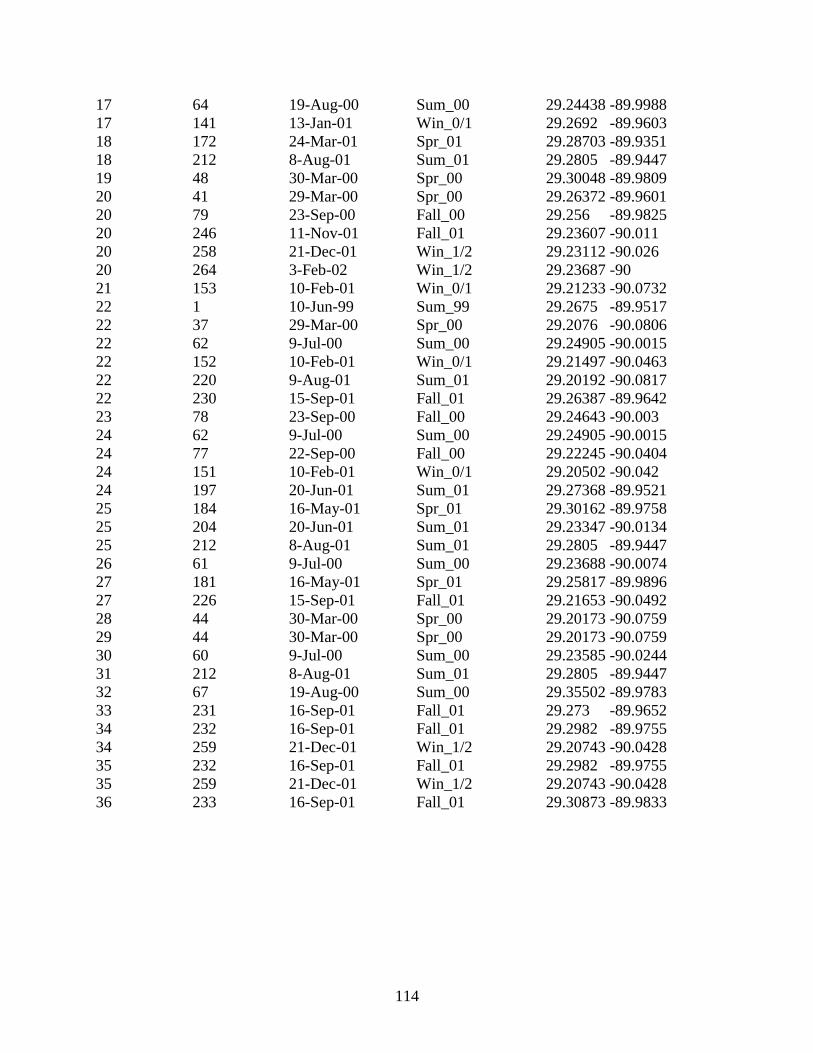
114
17 64 19-Aug-00 Sum_00 29.24438 -89.9988 17 141 13-Jan-01 Win_0/1 29.2692 -89.9603 18 172 24-Mar-01 Spr_01 29.28703 -89.9351 18 212 8-Aug-01 Sum_01 29.2805 -89.9447 19 48 30-Mar-00 Spr_00 29.30048 -89.9809 20 41 29-Mar-00 Spr_00 29.26372 -89.9601 20 79 23-Sep-00 Fall_00 29.256 -89.9825 20 246 11-Nov-01 Fall_01 29.23607 -90.011 20 258 21-Dec-01 Win_1/2 29.23112 -90.026 20 264 3-Feb-02 Win_1/2 29.23687 -90 21 153 10-Feb-01 Win_0/1 29.21233 -90.0732 22 1 10-Jun-99 Sum_99 29.2675 -89.9517 22 37 29-Mar-00 Spr_00 29.2076 -90.0806 22 62 9-Jul-00 Sum_00 29.24905 -90.0015 22 152 10-Feb-01 Win_0/1 29.21497 -90.0463 22 220 9-Aug-01 Sum_01 29.20192 -90.0817 22 230 15-Sep-01 Fall_01 29.26387 -89.9642 23 78 23-Sep-00 Fall_00 29.24643 -90.003 24 62 9-Jul-00 Sum_00 29.24905 -90.0015 24 77 22-Sep-00 Fall_00 29.22245 -90.0404 24 151 10-Feb-01 Win_0/1 29.20502 -90.042 24 197 20-Jun-01 Sum_01 29.27368 -89.9521 25 184 16-May-01 Spr_01 29.30162 -89.9758 25 204 20-Jun-01 Sum_01 29.23347 -90.0134 25 212 8-Aug-01 Sum_01 29.2805 -89.9447 26 61 9-Jul-00 Sum_00 29.23688 -90.0074 27 181 16-May-01 Spr_01 29.25817 -89.9896 27 226 15-Sep-01 Fall_01 29.21653 -90.0492 28 44 30-Mar-00 Spr_00 29.20173 -90.0759 29 44 30-Mar-00 Spr_00 29.20173 -90.0759 30 60 9-Jul-00 Sum_00 29.23585 -90.0244 31 212 8-Aug-01 Sum_01 29.2805 -89.9447 32 67 19-Aug-00 Sum_00 29.35502 -89.9783 33 231 16-Sep-01 Fall_01 29.273 -89.9652 34 232 16-Sep-01 Fall_01 29.2982 -89.9755 34 259 21-Dec-01 Win_1/2 29.20743 -90.0428 35 232 16-Sep-01 Fall_01 29.2982 -89.9755 35 259 21-Dec-01 Win_1/2 29.20743 -90.0428 36 233 16-Sep-01 Fall_01 29.30873 -89.9833
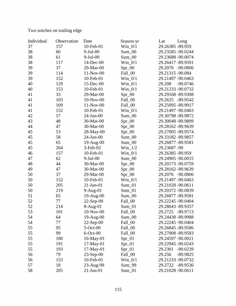
115
Two notches on trailing edge
Individual Observation Date Season-yr Lat Long 37 157 10-Feb-01 Win_0/1 29.26385 -89.959 38 60 9-Jul-00 Sum_00 29.23585 -90.0244 38 61 9-Jul-00 Sum_00 29.23688 -90.0074 38 117 14-Dec-00 Win_0/1 29.26417 -89.9591 39 37 29-Mar-00 Spr_00 29.2076 -90.0806 39 114 11-Nov-00 Fall_00 29.21315 -90.084 39 152 10-Feb-01 Win_0/1 29.21497 -90.0463 40 129 15-Dec-00 Win_0/1 29.208 -90.0746 40 153 10-Feb-01 Win_0/1 29.21233 -90.0732 41 33 29-Mar-00 Spr_00 29.29168 -89.9308 41 103 10-Nov-00 Fall_00 29.2625 -89.9542 41 109 11-Nov-00 Fall_00 29.25095 -89.9917 41 152 10-Feb-01 Win_0/1 29.21497 -90.0463 42 57 24-Jun-00 Sum_00 29.30798 -89.9872 43 48 30-Mar-00 Spr_00 29.30048 -89.9809 44 47 30-Mar-00 Spr_00 29.28162 -89.9639 45 53 28-May-00 Spr_00 29.27005 -89.9574 45 58 24-Jun-00 Sum_00 29.33182 -89.9857 45 65 19-Aug-00 Sum_00 29.26877 -89.9581 45 264 3-Feb-02 Win_1/2 29.23687 -90 46 157 10-Feb-01 Win_0/1 29.26385 -89.959 47 62 9-Jul-00 Sum_00 29.24905 -90.0015 48 44 30-Mar-00 Spr_00 29.20173 -90.0759 49 47 30-Mar-00 Spr_00 29.28162 -89.9639 50 37 29-Mar-00 Spr_00 29.2076 -90.0806 50 152 10-Feb-01 Win_0/1 29.21497 -90.0463 50 205 21-Jun-01 Sum_01 29.21028 -90.0611 50 219 9-Aug-01 Sum_01 29.20372 -90.0839 51 65 19-Aug-00 Sum_00 29.26877 -89.9581 52 77 22-Sep-00 Fall_00 29.22245 -90.0404 52 214 8-Aug-01 Sum_01 29.28643 -89.9357 53 101 10-Nov-00 Fall_00 29.2725 -89.9713 54 64 19-Aug-00 Sum_00 29.24438 -89.9988 54 77 22-Sep-00 Fall_00 29.22245 -90.0404 55 95 5-Oct-00 Fall_00 29.26845 -89.9586 55 99 6-Oct-00 Fall_00 29.27008 -89.9583 55 180 16-May-01 Spr_01 29.24597 -90.0021 55 191 17-May-01 Spr_01 29.22945 -90.0243 55 193 17-May-01 Spr_01 29.2301 -90.0239 56 79 23-Sep-00 Fall_00 29.256 -89.9825 56 153 10-Feb-01 Win_0/1 29.21233 -90.0732 57 18 23-Aug-99 Sum_99 29.2722 -89.9536 58 205 21-Jun-01 Sum_01 29.21028 -90.0611
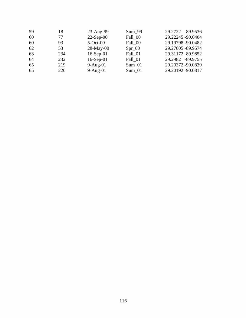
116
59 18 23-Aug-99 Sum_99 29.2722 -89.9536 60 77 22-Sep-00 Fall_00 29.22245 -90.0404 60 93 5-Oct-00 Fall_00 29.19798 -90.0482 62 53 28-May-00 Spr_00 29.27005 -89.9574 63 234 16-Sep-01 Fall_01 29.31172 -89.9852 64 232 16-Sep-01 Fall_01 29.2982 -89.9755 65 219 9-Aug-01 Sum_01 29.20372 -90.0839 65 220 9-Aug-01 Sum_01 29.20192 -90.0817
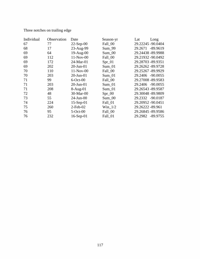
117
Three notches on trailing edge
Individual Observation Date Season-yr Lat Long 67 77 22-Sep-00 Fall_00 29.22245 -90.0404 68 17 23-Aug-99 Sum_99 29.2671 -89.9619 69 64 19-Aug-00 Sum_00 29.24438 -89.9988 69 112 11-Nov-00 Fall_00 29.21932 -90.0492 69 172 24-Mar-01 Spr_01 29.28703 -89.9351 69 202 20-Jun-01 Sum_01 29.26262 -89.9728 70 110 11-Nov-00 Fall_00 29.25267 -89.9929 70 203 20-Jun-01 Sum_01 29.2406 -90.0055 71 99 6-Oct-00 Fall_00 29.27008 -89.9583 71 203 20-Jun-01 Sum_01 29.2406 -90.0055 71 208 8-Aug-01 Sum_01 29.26543 -89.9587 72 48 30-Mar-00 Spr_00 29.30048 -89.9809 73 55 24-Jun-00 Sum_00 29.2332 -90.0187 74 224 15-Sep-01 Fall_01 29.20952 -90.0451 75 260 2-Feb-02 Win_1/2 29.26222 -89.961 76 95 5-Oct-00 Fall_00 29.26845 -89.9586 76 232 16-Sep-01 Fall_01 29.2982 -89.9755
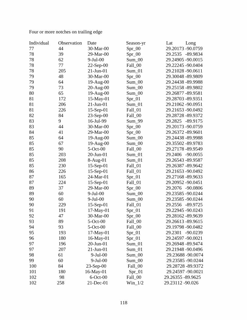
118
Four or more notches on trailing edge
Individual Observation Date Season-yr Lat Long 77 44 30-Mar-00 Spr_00 29.20173 -90.0759 78 39 29-Mar-00 Spr_00 29.2535 -89.9834 78 62 9-Jul-00 Sum_00 29.24905 -90.0015 78 77 22-Sep-00 Fall_00 29.22245 -90.0404 78 205 21-Jun-01 Sum_01 29.21028 -90.0611 79 48 30-Mar-00 Spr_00 29.30048 -89.9809 79 64 19-Aug-00 Sum_00 29.24438 -89.9988 79 73 20-Aug-00 Sum_00 29.25158 -89.9802 80 65 19-Aug-00 Sum_00 29.26877 -89.9581 81 172 15-May-01 Spr_01 29.28703 -89.9351 81 206 21-Jun-01 Sum_01 29.21062 -90.0951 81 226 15-Sep-01 Fall_01 29.21653 -90.0492 82 84 23-Sep-00 Fall_00 29.28728 -89.9372 83 9 16-Jul-99 Sum_99 29.2825 -89.9175 83 44 30-Mar-00 Spr_00 29.20173 -90.0759 84 41 29-Mar-00 Spr_00 29.26372 -89.9601 85 64 19-Aug-00 Sum_00 29.24438 -89.9988 85 67 19-Aug-00 Sum_00 29.35502 -89.9783 85 90 5-Oct-00 Fall_00 29.27178 -89.9549 85 203 20-Jun-01 Sum_01 29.2406 -90.0055 85 208 8-Aug-01 Sum_01 29.26543 -89.9587 85 230 15-Sep-01 Fall_01 29.26387 -89.9642 86 226 15-Sep-01 Fall_01 29.21653 -90.0492 87 165 24-Mar-01 Spr_01 29.27168 -89.9633 87 224 15-Sep-01 Fall_01 29.20952 -90.0451 89 37 29-Mar-00 Spr_00 29.2076 -90.0806 89 60 9-Jul-00 Sum_00 29.23585 -90.0244 90 60 9-Jul-00 Sum_00 29.23585 -90.0244 90 229 15-Sep-01 Fall_01 29.2556 -89.9725 91 191 17-May-01 Spr_01 29.22945 -90.0243 92 47 30-Mar-00 Spr_00 29.28162 -89.9639 93 89 5-Oct-00 Fall_00 29.26613 -89.9615 94 93 5-Oct-00 Fall_00 29.19798 -90.0482 95 193 17-May-01 Spr_01 29.2301 -90.0239 96 180 16-May-01 Spr_01 29.24597 -90.0021 97 196 20-Jun-01 Sum_01 29.26948 -89.9474 97 207 21-Jun-01 Sum_01 29.21948 -90.0496 98 61 9-Jul-00 Sum_00 29.23688 -90.0074 99 60 9-Jul-00 Sum_00 29.23585 -90.0244 100 84 23-Sep-00 Fall_00 29.28728 -89.9372 101 180 16-May-01 Spr_01 29.24597 -90.0021 102 98 6-Oct-00 Fall_00 29.26355 -89.9625 102 258 21-Dec-01 Win_1/2 29.23112 -90.026

119
103 64 19-Aug-00 Sum_00 29.24438 -89.9988 104 64 19-Aug-00 Sum_00 29.24438 -89.9988 105 64 19-Aug-00 Sum_00 29.24438 -89.9988 106 98 6-Oct-00 Fall_00 29.26355 -89.9625
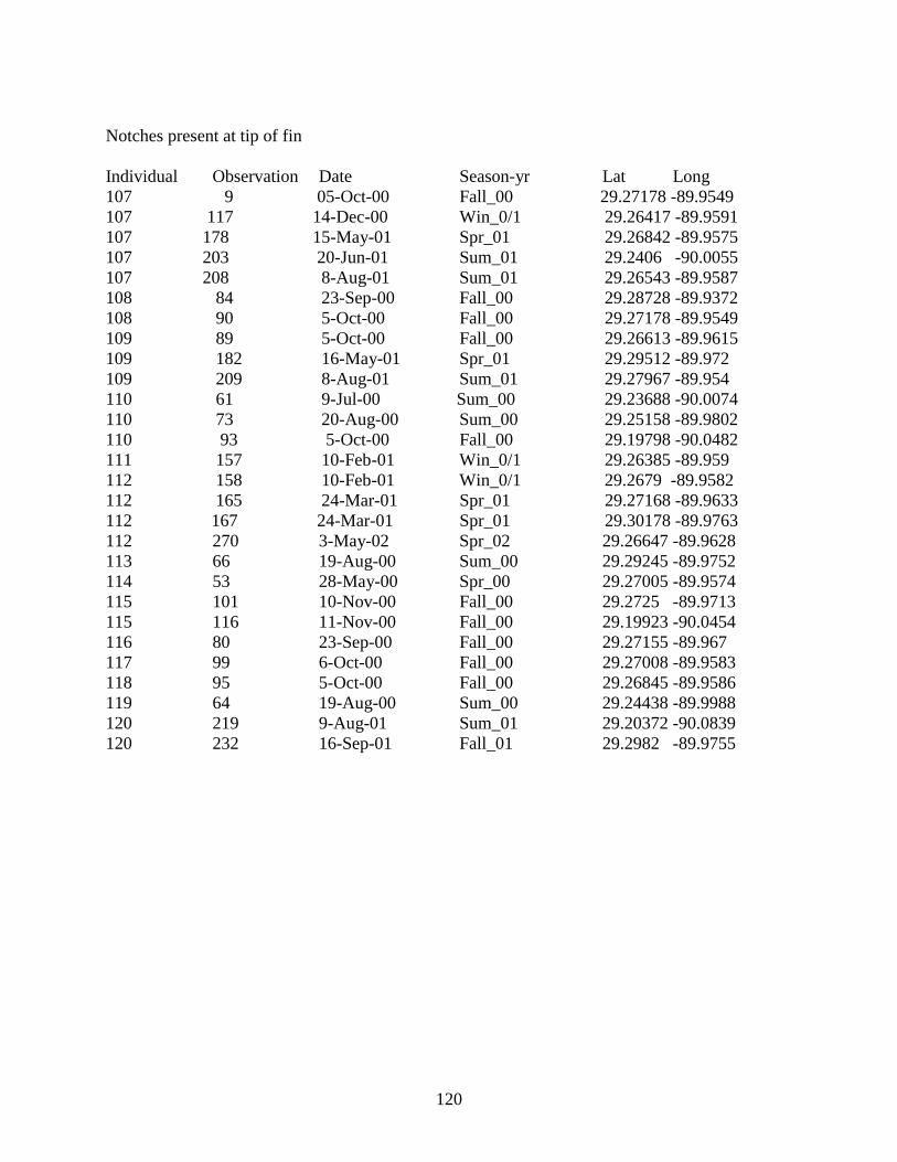
120
Notches present at tip of fin Individual Observation Date Season-yr Lat Long 107 9 05-Oct-00 Fall_00 29.27178 -89.9549 107 117 14-Dec-00 Win_0/1 29.26417 -89.9591 107 178 15-May-01 Spr_01 29.26842 -89.9575 107 203 20-Jun-01 Sum_01 29.2406 -90.0055 107 208 8-Aug-01 Sum_01 29.26543 -89.9587 108 84 23-Sep-00 Fall_00 29.28728 -89.9372 108 90 5-Oct-00 Fall_00 29.27178 -89.9549 109 89 5-Oct-00 Fall_00 29.26613 -89.9615 109 182 16-May-01 Spr_01 29.29512 -89.972 109 209 8-Aug-01 Sum_01 29.27967 -89.954 110 61 9-Jul-00 Sum_00 29.23688 -90.0074 110 73 20-Aug-00 Sum_00 29.25158 -89.9802 110 93 5-Oct-00 Fall_00 29.19798 -90.0482 111 157 10-Feb-01 Win_0/1 29.26385 -89.959 112 158 10-Feb-01 Win_0/1 29.2679 -89.9582 112 165 24-Mar-01 Spr_01 29.27168 -89.9633 112 167 24-Mar-01 Spr_01 29.30178 -89.9763 112 270 3-May-02 Spr_02 29.26647 -89.9628 113 66 19-Aug-00 Sum_00 29.29245 -89.9752 114 53 28-May-00 Spr_00 29.27005 -89.9574 115 101 10-Nov-00 Fall_00 29.2725 -89.9713 115 116 11-Nov-00 Fall_00 29.19923 -90.0454 116 80 23-Sep-00 Fall_00 29.27155 -89.967 117 99 6-Oct-00 Fall_00 29.27008 -89.9583 118 95 5-Oct-00 Fall_00 29.26845 -89.9586 119 64 19-Aug-00 Sum_00 29.24438 -89.9988 120 219 9-Aug-01 Sum_01 29.20372 -90.0839 120 232 16-Sep-01 Fall_01 29.2982 -89.9755
121
Notches present on leading edge
Individual Observation Date Season-yr Lat Long 121 55 24-Jun-00 Sum_00 29.2332 -90.0187 121 154 10-Feb-01 Win_0/1 29.1968 -90.0837 121 194 17-May-01 Spr_01 29.24932 -89.988 121 226 15-Sep-01 Fall_01 29.21653 -90.0492 121 251 20-Dec-01 Win_1/2 29.21628 -90.0493 122 204 20-Jun-01 Sum_01 29.23347 -90.0134 122 219 9-Aug-01 Sum_01 29.20372 -90.0839 123 251 20-Dec-01 Win_1/2 29.21628 -90.0493 124 151 10-Feb-01 Win_0/1 29.20502 -90.042 125 44 30-Mar-00 Spr_00 29.20173 -90.0759 126 169 24-Mar-01 Spr_01 29.34215 -89.9847 126 170 24-Mar-01 Spr_01 29.3543 -89.9687 127 1 10-Jun-99 Sum_99 29.2675 -89.9517 128 195 20-Jun-01 Sum_01 29.26647 -89.9628 129 53 28-May-00 Spr_00 29.27005 -89.9574 130 18 23-Aug-99 Sum_99 29.2722 -89.9536 131 63 9-Jul-00 Sum_00 29.26613 -89.9639 132 25 10-Dec-99 Win_9/0 29.2726 -89.9513 132 185 16-May-01 Spr_01 29.30913 -89.9822 132 197 20-Jun-01 Sum_01 29.27368 -89.9521 133 64 19-Aug-00 Sum_00 29.24438 -89.9988 134 93 5-Oct-00 Fall_00 29.19798 -90.0482 134 101 10-Nov-00 Fall_00 29.2725 -89.9713 135 112 11-Nov-00 Fall_00 29.21932 -90.0492 135 150 10-Feb-01 Win_0/1 29.20493 -90.0446
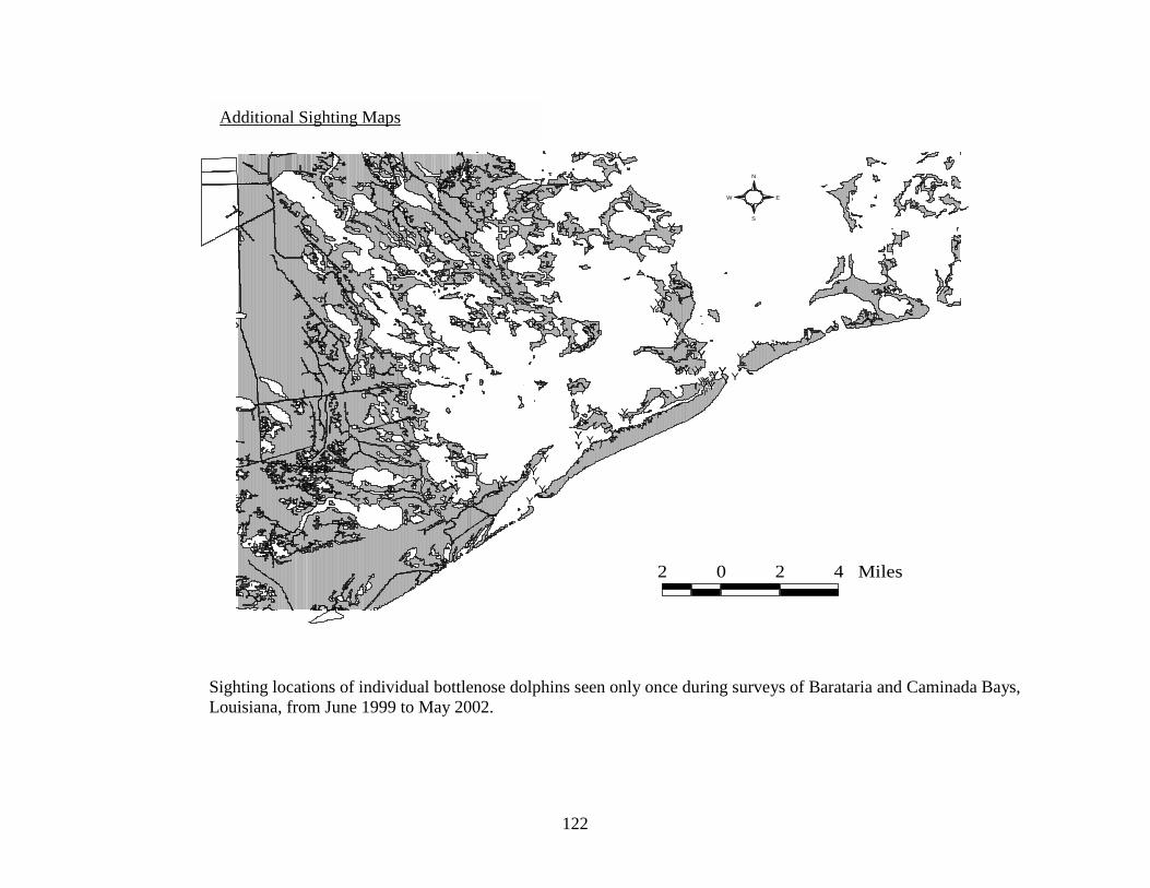
122
#Y
#Y
#Y
#Y
#Y#Y
#Y
#Y
#Y
#Y
#Y
#Y
#Y
#Y
#Y
#Y
#Y
#Y
#Y
#Y#Y #Y
#Y
#Y#Y
#Y
#Y
#Y
#Y
#Y
#Y
#Y
#Y
#Y
#Y
#Y
#Y
#Y
#Y
#Y
#Y
#Y
#Y
#Y
#Y
#Y
#Y#Y
#Y
#Y#Y#Y#Y
#Y#Y
#Y
#Y#Y#Y #Y#Y
#Y
#Y
#Y#Y
#Y
#Y#Y#Y#Y
#Y
#Y
#Y
#Y
#Y
#Y
#Y
#Y
2 0 2 4 Miles
S
N
EW
Sighting locations of individual bottlenose dolphins seen only once during surveys of Barataria and Caminada Bays, Louisiana, from June 1999 to May 2002.
Additional Sighting Maps
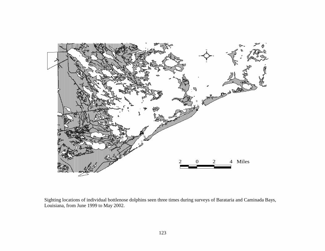
123
#
##
%%
%
#³
#³
#³
#S
#S
#S
ââ â
&V
&V
&V
#Y
#Y
#Y
%[
%[%[
#
#
#
$
$
$
xzxzxz
#·
#·
#·
2 0 2 4 Miles
S
N
EW
Sighting locations of individual bottlenose dolphins seen three times during surveys of Barataria and Caminada Bays, Louisiana, from June 1999 to May 2002.
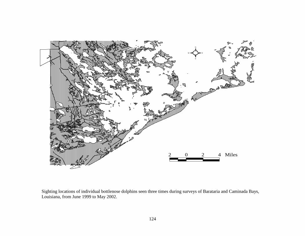
124
#Y
#Y
#Y
#Y
&
&&
&
$
$
$
$
#³
#³
#³
#³
%a%a
%a
%a
#
#
#
#
Ú
Ú
Ú
ÚÚ
#0
#0#0
#0
#0
%[
%[
%[
%[%[
%
%
%%
%
#S
#S
#S
#S
#S
#S
2 0 2 4 Miles
S
N
EW
Sighting locations of individual bottlenose dolphins seen three times during surveys of Barataria and Caminada Bays, Louisiana, from June 1999 to May 2002.
125
VITA
Cara Miller was born in Stirling, South Australia, on July 8th 1975. She is the daughter of
Robert Miller and Donna Gavin and the younger sister of Robin Tuan. She attended
Heathfield High School in the Adelaide Hills, finishing in 1992. The following year Cara
accepted a tennis scholarship to Lewis-Clark State College in Idaho. At the start of her
junior year she transferred to the University of Portland, Oregon, where she received a
Bachelor of Science degree in life science in May 1997. After graduation Cara moved to
Alaska and worked as a fisheries biologist for the National Marine Fisheries Service.
This experience confirmed her interest in pursuing a graduate degree in the marine
sciences. She entered the Department of Oceanography and Coastal Sciences at
Louisiana State University in the fall of 1998 with a Board of Regents fellowship. While
pursuing her doctoral degree, she completed a master’s degree in applied statistics in May
2002 with advisor Dr. E. Barry Moser. She will earn her doctoral degree in oceanography
and coastal sciences in December 2003 under the supervision of Donald M. Baltz.