AC-016? 346 A NEW EFFICIENT APPROACH TO THE FORMULATION OF MIXED 1i/1FINITE ELEMENT NODEL.. (U) NRYAND UNIV COLLEGE PARKDEPT OF AEROSPACE ENGINEERING 5 W LEE ET AL. FEB 96

UNCLASSIFIED N84- -0205 B F /6 29/11NL

.

2.8.

L L36 *

M'CR(OOF CHART

CCD

A NEW EFFICIENT APPROACH TO THE FORMULATION

OF MIXED FINITE ELEMENT MODELS FOR STRUCTURAL ANALYSIS A

S.W. LEE

-~J.J. RHlU DINi A.y is

February 1936

INTERIM REPORT B .

Office of Naval ResearchContract No. NOU'34-34-K-0385.

Work Unit No. NRO64-718/4-6-84,432S)

PPROVE) FOR PUBLIC RELEASE: DIST-4IUTION UNLIMITED

-4cassifi edtjCR C.ASSIFICAION of TIS PAGE ,

REPORT DOCUMENTATION PAGE60 1I'A E.RT C.SIIAINlb RESTRICTIVE MARKINGS

Unclassified~SECURIT~ CLASSIFICATION AUTMORITV 3. OSTRI~uTIONIAVAILABiLITY OF REPORT

DIE OECLAS&IPFSCAT IONIGOV0NGRADI N6SCHSOULS Unlimited

. Of, RFOPMING ORGANIZATION REPORT kUMSEM(SI 6. MONITORING ORGANIIZATION REPORT NUMIERIS)

6 IMOFPERFORMING ORGANIZATION 0.b OFFICE SYMBOL 7&. NAME OP MONITORING ORGANIZATION I~

Department of Aerospace Eng. I 16 eDda"ble) Office of Naval R~searchUniversity of Maryland ________ Mechanics Division

69. ALOORESS (Ci. S8416 and ZIP Code) 7b. ADDRESS 108y3. Staae. .d ZIP Code#

800 North Quincy StreetCollege Park, Maryland 20742 Arlington, VA 22217

B.. NAME OF FUNOING/SPONSORING 46. OFF ICE SYMBOL B.PROCUREMENT INSTRUMENT IDENTIFICATION4 NUMSERORGANIZATION i elabuOffice of Naval Research N00014-84- K;0385

J6. ADORESS IC~ty. State and ZIP COO)S 10. SOURCE OP FUNDING NOS.

800 North Quincy Street PROGRAM PROJECT TASK WORK UNITArlington, VA 22217 ELE.1MINT NO. Ndo. No. NO.] NR064-7181

'. TITL~M~bEScnCaaaiemg A New Ef f icien Appr aht hFormulation of Mixed Finite Element Models or Structural Analysis4-8(32)

12. PERSONAL AUTMORIS.W. Lee and 3.3. Rhiu

3.TEOPREPORT 131L TIM5 COWRj 4. DATE OF REPORT IV.. N&.. Day) is. PAGE COUNT

interim FROM _ay J% Td une_ 1 40 F Feb 1986 1 30iS. SUPPLEMENTARY NOTATION

II,.COSATI COOES IS& SUBJE CT TSERMS IComimanua Aon If~, Unee~oay ond ientify by bleea num~oiPI. ROP Sun. GR. new mixed formulation, Hellinger-Reissner principle,

FIEO GRUPlower order and higher order assumed strain

10g. ABSTRACT Wonfnauo on Moojr" o tnoeerv and itdalty by blok number

CC / A new finite element formulation is developed based on the~.Hellinger-Reissner principle with independent strain. By dividing the assumedstrain into the lower order part and the higher order part, the new formulationcan be imade much more efficient than the standard mixed formulation. In additionIthe present new approach provides a rational way of introducing stabilizationmatrix to suppress undesirable kinematic modes.

OISTRIBUTIONIAVAILAIILiTv OP ABSTRACT 21. ABSTRACT SECURITY CLASSIFICATION

UNCLASSIPIEOIUNLIMITEO 0 SAME AS APT. 0 OTIC USERS 0j unclassified..a. NAME OP RESPONS2I INDIVIDUAL 226 TELEPtIOP4 NUMBER 22.. OFF ICE SYMBOL

Dr. R.E. Whitehead, Mechanics Division, ONR (Inclue-A96e-43de

FORM 1473, 83 APR EDITION OF 1.#AN 73 IS OBSOLETE. uncl assi fiedSECURITY CLASSIFICATION OF T04-S PAGE

-, S - . -o-

A NEW EFFICIENT APPROACH TO THE FORMULATION

OF MIXED FINITE ELEMENT MODELS FOR STRUCTURAL ANALYSIS

S.W. LEE

J.J. RHIU

February 1986

INTERIM REPORT

Office of Naval ResearchContract No. NOO014-84-K-0385

Work Unit No. NR064-718/4-6-84(432S)

APPROVED FOR PUBLIC RELEASE: DISTRIBUTION UNLIMITED

.-%- 7.- 4

IL"-. - .'.' ,".'.- ; '. -. _'. ''..''.' '- *, ,S '*S* *"5''**,''S*'- **-'"5. . ...... " "... ."' ...- -. . . . .-- "

If

SUMMARY

A new mixed finite element formulation is developed based on the

Hellinger-Reissner principle with independent strain. By dividing the assumed

strain into the lower order part and the higher order part, the new formulation

can be made much more efficient than the standard mixed formulation. In addi- • '

tion the present new approach provides an alternative way of introducing stabi- -'

lization matrix to suppress undesirable kinematic modes.

Accession ~ - -TIS GR.'.'

DTIC TAr%

Jus.

• =Av,.

LI.°,. ..

~~~~... . . . . . . . . . . .. . . .. *"..'-.°

1. INTRODUCTION

Hybrid and mixed finite element formulations based on the

Hellinger-Reissner principle or related variational principles have been

available since the early days in the history of finite element method [1]. In

these formulations an independent stress or strain is assumed within an element

in addition to the usual assumed displacement expressed in terms of nodal

displacement. The independent stress or strain is eliminated at element level,

resulting in an element stiffness matrix corresponding to nodal displacement

vector. Note that in this paper we are not interested in the type of mixed for-

mulation used in reference 9 where both nodal displacements and nodal stress

variables remain in the assembled global model. For an element with a given

-' number of nodes there is a degree of flexibility in the choice of assumed stress

or strain. For example in the case of Pian's original assumed scress hybrid

model (2], the assumed stress is chosen to satisfy equilibrium within an ele-

ment. Of course, the property of the stiffness matrix depends very much on the

assumed stress or strain. Thus with a proper choice of assumed stress or strain

it is possible to develop a finite element model which is superior to the con-

ventional finite element model based purely on the assumed displacement

approach. For example, for thin plates and shells, a mixed formulation based on

the Hellinger-Reissner principle or the modified Hellinger-Reissner principle

can be used to alleviate the undesirable locking effect associated with the con-

dition of zero inplane strain and zero transverse shear strain imposed on a

finite element model [3,41. The role of hybrid and mixed formulations in con-

junction with nearly incompressible materials has also been studied [5].

Moreover a mixed formulation provides a rational mathematical basis for the

popular reduced and selective integration scheme [6-81.

However. in hybrid and mixed formulations it is necessary to invert a

1 .

matrix in order to generate an element stiffness matrix. Therefore, in com-

parison with the assumed displacement model based on the principle of virtual

work, hybrid and mixed formulations require usually more time to compute element

stiffness matrix of the same size. This fact has been regarded as the major

drawback of the conventional hybrid and mixed formulations.

With this in mind, we present in this paper a new mixed formulation which

requires much less computing time than the conventional mixed formulation for

the generation of element stiffness matrix. The new formulation is based on the

Hellinger-Reissner principle with independent strain. The new formulation can

be applied to any type of problems in solid and structural mechanics. However,

for simplicity, two dimensional plane problems will be used to demonstrate the .

effectiveness of the approach. Initially nine node element will be used for the...purpose of illustration. A short discussion on four node element will follow. ,-,-..-

In order to contrast the new formulation with the conventional formulation, we

will start off with the conventional formulation.

2. CONVENTIONAL MIXED FORMULATION

2.1 Finite Element Formulation

For two dimensional plane problem, the functional IR for the

Hellinger-Reissner principle can be written as

f (T 1 iT ___-_

R (E Cc--f Cc) dA -W (1)

where exx

C: :yy } independent strain vector

2~. .... .... ....

-La vv

J- * lf 1 v strain vector in

EY a y Y terms of displace-,au vment field

xy ay aap "- '

u, v: displacement in x and y direction respectively

A: area

W: external load term

C: 3 x 3 matrix of elastic constants integrated through thickness

Note that in eg. (1) instead of stress, strain £ appears as independent

variables in addition to displacement field u and v.

For finite element approximation, the displacement vector u is assumed

in terms of nodal displacement vector as

U= N % (2)v-

where N: shape function matrix

ae: element nodal displacement vector

Then the strain vector c can be written symbolically as

= B qe (3)

where B is the matrix relating E to qe"

3%-'. .]

3 4°- " " .

---------------------------------------------------------------------. °.-- . .,° .°

In addition, within each element the independent strain c is assumed in terms of

unknown coefficients as

£=PC% (4)

where P: strain shape function matrices

a: vector of unknown coefficients in an element % b~e

Introducing eq. (3) and (4) into eq. (1). W

,T1IT T

with G= P TC BdA (5a)Ae

H PT C P dA (b

Ae

W T W = (5c)e Qe

and Ae is the element area.

The summation sign indicates summation or assembly over all elements.

Taking 5 R=0 with respect a in each element,

G q -H =0 (6) ~.t

or solving for c,

a H G q (7) 77

for each element.

4

Substituting eq. (7) into eq. (5), WR is written as

1R( 2T % e T (8)

where K = GT H-1G (9)

is the element stiffness matrix.

Assembling over all elements,

1 T T °'

1R = w K 2 - q2 (10)

where K: global stiffness matrix

L: global nodal displacement vector 22: global load vector .*

Setting "R 0 with respect to leads to

K g. (11) "

which can be solved for . With thus e known, the independent strain

vector c in an element is determined by substituting eq. (7) to eq. (9)

such that

: P Se (12)

and for isotropic materials, stress ~ is determined as follows:

S iCc (13)

where t is the thickness.

5,-"- , ;.i1- -

• ..- . -. e•.%. ,• -*• ."•*-. . ." o %"" . """. "" " " . .""" ." . ."" " .. "+ " " + " "". .', . . , m ,. , .- . - . . -

+ . + ,+ , ,+ I - ' , ", .. . • m L -- ' - + - - - - - + -.

2.2 Nine Node Element

The present nine node element is important in that it constitutes

inplane part of the nine node shell element described in reference 4. This

particular shell element has been found to be free of locking and any com-

patible or commutable kinematic mode. Of course a good nine node ele-

ment is useful for plane stress and plane strain analysis itself. For the..

assumed displacement, the element shown in fig. 1 adopts the isoparametric

representation. As for the coordinate system, global and local cartesian

coordinate systems are used. The strains c, £ and displacement u,v in eq.

(1) are defined with respect to the global coordinate system. Local coor-

6 dinate system is introduced to allow an assumed strain field with nonsymmetric

polynomial terms. Local coordinate system is defined first by

determining two unit vectors v1 and v at - = 0 point such that

a'.,% /

2 a a- (14)

where x is the position vector with components in the global coordinate

system. The angle 00 between these two unit vectors is calculated from the

following equation: -'

cose o = vI •2 (15)

6.............- .*....-.** * *. .... ...-.-. ..-- *

.1. ..- :

Then, if o is less than or equal to 900, unit vector a in the x direction

of local coordinate system is defined as

ax / a4al (16)

Otherwise a1 is defined as

ax /axan an (17)

Unit vector a2 in the y direction of local coordinate system is orthogonal

to a1. Note that, while v1 and Y2 are determined at E = n = 0 point, a1

and a can be computed at any point in the element. Especially aI and a2

are needed at integration points to establish a local orthogonal coordinate

system. Now, for the present nine node element, we may assume the indepen-

dent strain in local coordinate system as follows;

xx + a2& + a3n + a4" + al3fx

Cyy =a 5 + a6 + a7n + a8"n + a14 fy (18)

£xy =9 + lO1 + a1 1n + a1 2"

In eq. (18), fx = n2 and fy = E n for 21 defined as in eq. (16). For aI de-

fined as in eq. (17), f and fy are chosen as fx = n and fy = Note

that, due to the a13 and a14 terms, the assumed strains are not symmetric in E

and n. However with the use of local coordinate system as defined here, the

resulting stiffness matrix will not be dependent upon the choice of global coor-

dinate system. Symbolically eq. (18) can be written as .- -

P* (19)

7

. . .

.- . -. . - ,'... -.-. .% . ; . ... *,...-..-.-.-. a ta A F fla- -.- , .,.- - . .- -. ".',"-" ',. .".- - " "'. :

5, ----- - -- q. .' ~ ~ '

- ....... " .

Lxx

where (19~La)

.-, -

and ~= a ± 2 * " (19b)

is the column vector of unknown strain coefficients, and P is the 3 x 14

matrix containing polynomial terms in & and n coordinates. The strain vec-

tor £ in global coordinate system is obtained from c through strain trans-

formation matrix T as follows:

c T = T P a P a (20)

where P =T P (20a)

As shown in eq. (9), for the generation of element stiffness matrix, it is

necessary to compute G and H-• For the present nine node element the size

of G and H matrices are 14 x 18 and 14 x 14 respectively and G and H matrices

are evaluated using 3 x 3 point Gaussian quadrature. As far as computung

time is concerned the need to evaluate G, H and H "1 makes the conventional

mixed formulation less attractive than the assumed displacement formulation

based on the principle of virtual work.

At this point, it is well to mention that the a13 and a14 terms in eq.

(18) were chosen carefully to suppress undesirable kinematic modes.

Without the a13 and '14 terms, the assumed strain field is symmetric in e

and n. Moreover, for an element of rectangular shape, 2 x 2 point rule is

sufficient enough for exact integration of G and H. Then the resulting

8 _

I . - ' "

stiffness matrix will be equivalent to the conventional assumed displace-

ment model with 2 x 2 reduced integration. The equivalence between mixed

formulation element and reduced or selective integration element can be

proved by establishing

(21)

at integration points. This can be done if the number of integration

points is the same as the number of strain parameters or coefficients in

each component of assumed strain 13,6,71. The element without the a13 and

¢14 terms exhibits three kinematic modes or spurious zero strain enery

modes. For a square element with sides along x = ±1 and y = +1 lines,

these spurious modes are as follows [10,11];

(1) u = C1x(1 3yz )

v = -Cly(1 - 3x2 ) (22)

(2) u = C2(x2 + y -- 3x~yZ)

(3) v = C3(xZ + y -. 3xzyz)

where C1 , C2 and C3 are arbitrary constants. Among these three modes, the

first mode is incompatible or non-commutable as it disappears for an

assembly of only two elements. The second and third modes are compatible

or commutable and may persist even after assembly of elements, resulting in.-.,

an unstable finite element model. The a13 and a14 terms in the assumed

strain are introduced to suppress these two compatible modes. The first

mode is left in the element since it is harmless. It is to be noted that

the same assumed strain was used in the shell element described in

reference 4 where it was found to be very effective in alleviating locking

effect associated with the condition of zero inplane strain.

9

. . . . . . .. ............ ...9~~ -n. -1.

3. NEW FORMULATION

The proposed new formulation is also based on the Hellinger-Reissner

principle with the functional given in eq. (1). However in the new for-

mulation, the independent strain is written as

C =L C (23) 1M

where L is the independent strain vector with lower order polynomial terms

in g and n. On the other hand £H' the higher order strain vector, contains

higher order terms in E and n. More discussion on £L and cH will be given

later. Inserting eq. (23) into eq. (1), the functional R becomes

- TR= f C C e dA

dAc - ~H -CC d

1iTf7 £H C cHdA - W (24) *'.',

To help illustrate the new formulation, we will consider again nine node

element. For nine node element of rectangular shape, the highest order

terms in the e matrix are quadratic in either E or n direction. Thus if the

L matrix is bilinear, then the first integral can be integrated exactly

using 2 x 2 point Gaussian quadrature. For £H' we start by assuming H.,

the higher order strain vector in the local coordinate system, as -

=xx)H aifx

(y) = 2fy (25)(y)H 0

(cXY)H 0

10

. . . 4 . . . . . . , ,, , . -. . , . . ...- . ,, -. . . ... .-.-.- . :. . , -. ::. :,--..- -:,,-,, . 4 . ' . . ' . " . ., ,P. " . . . . . . . '.. ," ****'*," ." . . .* ,. . --, . *4{, .'.", • *- , * ,9","_,- z

Or in matrix form, =

£H = (26)

where -

f 0

* 0 fy (26a)

0 0

~ 2(26b)

*2

Note that eH contains the higher order a13 and a14 terms of the conventional

formulation given in the previous section. Using the strain transformation

matrix T, the £H vector in the global coordinate system is expressed as

H= T £H = T a = (27)

where T P (27a) -... '

Of course, for rectangular element, T is equal to P. However, for an ele-

ment of arbitrary shape, strain transformation in eq. (27) is used. Again,

for rectangular element, the third integrals in eq. (24) require 2 x 2

, point rule. On the other hand the second and fourth integrals require 3 x

3 point rule. For an element with arbitrary shape the argument regarding

the number of integration points for exact integration does not hold.

However even in this case the same integration rules will be adopted.. :

* 11 o

. ., .,

-' ., , , . . • . ° . - .V. . . - . . . , .- . - . ,- . - - - : . .. - . .. _,

,.~) ,j , jt'S ,b ~~ ~Wj. : iL, ~ ~ ,, , i . '.. T ... ' , L, . J,1. I,' . *. , i } - i:' -. ,i- . 'j 'M

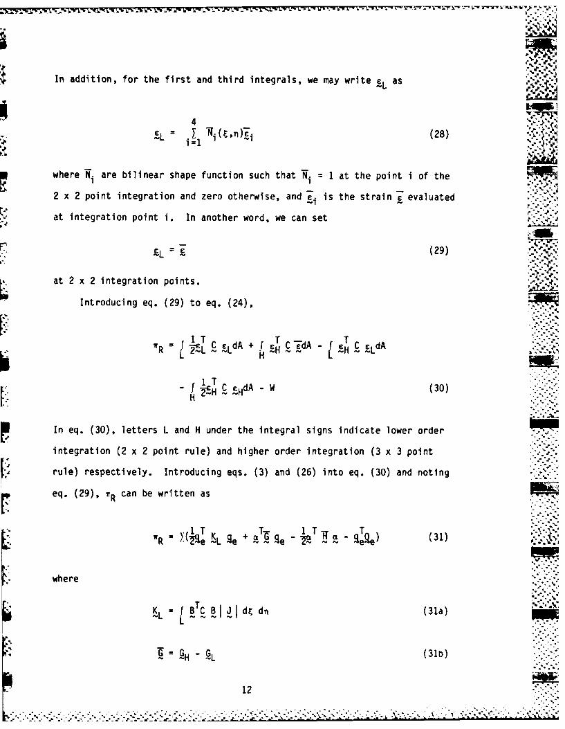
In addition, for the first and third integrals, we may write C L as t..1

L (E'n)gi (28)

where Ni are bilinear shape function such that Ni 1 at the point i of the

2 x 2 point integration and zero otherwise, and ci is the strain c evaluated .- - "i.. ,, p"

at integration point i. In another word, we can set

L= (29) .

at 2 x 2 integration points.

, L

Introducing eq. (29) to eq. (24),

" f + TC'= L H d -H, Ld

1 T -'''-

-- C HdA - W (30)

In eq. (30), letters L and H under the integral signs indicate lower orderJ

integration (2 x 2 point rule) and higher order integration (3 x 3 point

rule) respectively. Introducing eqs. (3) and (26) into eq. (30) and noting

eq. (29), iR can be written as

1 Y(e KT + 1 T T e) (31)

where

11.

.N.

L BTC B J d& dn (31a)

-H -H L (31t))

12

°° . ° - j .- . . -o . • °° ., - - o , ° .-- ",-- , . • ... . ° - • ° . ° * o . o . • , •° .- +,• o o . •-

~~~~~~~~~o... . . . . . . . . . . . . . . .%'. . ..

G f £ BI d dn (31c) V

R= f pTC IFJ dt dn (39e)

andl JI is the determinant of Jacobian matrix J. Note that, although the

same symbol B appears in KL, GH and G B in G is evaluated at 3 x 3

Gaussian integration points while B in KL and G L is evaluated at 2 x 2

Gaussian integration points. However to save computing time, the B matrix

at 2 x 2 integration points can be interpolated from the B matrix evaluated

at 3 x 3 integration points. That is, we evaluate B at 2 x 2 points from the

following expression:

9

Li- ~B 1 (32)

where Bi is the B matrix at the integration point i and is the shape

function such that Ni =1 at point i of the 3 x 3 integration points and

zero at other points. In addition the determinant i at 2 x 2 integration

points is also interpolated from I J1 at 3 x 3 integration points.

Taking 5nR with respect to of each element ., -

- e = 0 (33)

A,. or solving for

for each element.

13

Substituting eq. (34) into eq. (31),

W I T Kqe T (5'R (35)Qe

where

K = G T-!- (36)Ke

is the element stiffness matrix. Assembling over all elements

WR _ TK 3 .TQ (37)

where K is the global stiffness matrix corresponding to the global displa-

cement vector and Q is the global load vector. Taking 6 rR = 0 with

respect to results in

K g(38)% . 4

which can be solved for 2. With and thus e known strain c is determined

from eqs. (23), (27), (28) and (34) as follows:

= L -H -L + P a : ' " " '

4 _

2 ei +i P H - (39)

* Then stress a is determined by eq. (13).

It should be pointed out that the element stiffness matrix in eq. (36)~T "';;'"-

has two components, KL and G H G. For an element of rectangular shape the

matrix is the same as the stiffness matrix of the conventional assumed

displacement model with 2 x 2 reduced integration. Again the equivalence is

established through eq. (29). Then the KL matrix has the same three kinematic

14

~~.......................... ........... ..... . .-.-... .... . ....... -.. '" "."L.' ,.• .'.' ,.-..'.-.;'..';-.' --.- ,. .- " -. '- ' "-"."."." ."" .""' ,. '-" ._.'- . . .-:- .'- . '.-.-. _' " "-...".:. ---

-,. °

modes given in eq. (22). With the addition of 'T T-1 - matrix, the compatible

kinematic modes are suppressed, leaving only the incompatible mode. Therefore,

as far as kinematic modes are concerned, both the conventional formulation and

1%%the new formulation result in the same incompatible mode. However element T

stiffness matrix from the new formulation is not exactly the same as that from

the conventional formulation. The size of G and IT matrices in the new for-

mulation are 2 x 18 and 2 x 2 respectively. Therefore, computation of the

GTH G matrix in the new formulation can be carried out without much effort.

Recall that in the conventional formulation, the sizes of~G and~H matrices are

14 x 18 and 14 x 14 respectively. Note also that the present element passes the

patch test.

4. COMPARATIVE NUMERICAL TEST

(a) Comparison of Computing Time

In order to evaluate computing efficiency of the new formulation, a

test was run in which stiffness matrix of single nine node element was com-

puted 40 times consecutively. Table 1 shows relative computing time for

different element types. Clearly the new mixed formulation element (NM)

requires much less computing time than the conventional mixed formulation ele-

ment (CM). Surprisingly the new mixed formulation takes less computing

time than the conventional assumed displacement element with 3 x 3 point

rule (DISP3). Of course the assumed displacement element with 2 x 2 point

rule (DISP2) takes the least time. However, as mentioned before, this element

has compatible kinematic modes and thus cannot be used in general stress

analysis.

(b) A Panel under a Horizontal Point Load

Figure 2 shows a rectangular panel subjected to a horizontal point load P.

15

it L.%.T.7 "..-

The panel is modeled by 2 x 12 mesh as shown in the figure. Two boundary con-

ditions are considered. In case 1, the left end is completely fixed. In case

2, the vertical displacements of the first, second, fourth and fifth nodes

along the left end are left unconstrained. The first case has been used in

references 13 and 14 to demonstrate the undesirable effect of spurious kinematic

modes on numerical solution. The pertinent data are as follows;

length L - 12m W

depth b - 2m

Poissons ratio v = 0.2

P/AE """

where E is the Young's modulus and A is the cross-sectional area. Table 2 lists

the nondimensional horizontal displacement calculated at the load point for the

NM, CM, DISP2 and DISP3 elements. Numerical solutions are nondimensionalized by

dividing the computed values by the tip displacement PL/AE of a panel under total

load P distributed uniformly over the cross-sectional area. The solution for the

DISP2 element is very large compared with those obtained by the other three ele-

ment types, especially in case 2. This is due to the spurious compatible kine- -

matic modes in the DISP2 element triggered by te point load. The NM, CM ele-

ments are free of compatible kinematic modes and the DISP3 element has no .

kinematic mode. Therefore they provide stable solutions.

(c) A Cantilever Beam

A cantilever beam subjected to a tip load P is used to evaluate the.

performance of the present new element as compared to the conventional mixed *.

formulation element and the assumed displacement model element. Note again that

the same problem has been used as a numerical example in reference 13. As

illustrated in fig. 3, the cantilever beam is modelled by three different :-". - -

16

------ ----- ------ -----

* - -- - - .

..

-I

finite element meshes. Two different length to depth ratios of 10 and 20

are considered. Table 3 lists computed vertical displacement of point A infig. 3 and stress a evaluated at point B. The point B is one of the

Gaussian points in the 2 x 2 integration rule. Numerical solutions were

normalized by the following solutions obtained from the Bernoulli-Euler

beam theory:

3vA - PL /3EI

(Uxx) B = M YB/ 1 (41)

where

I = sectional area moment of inertia

M = hending moment

B y coordinate of point B

Numerical results in Table 3 indicates that NM, CM and DISP2 elements perform

much better than the DISP3 element especially for meshes with non-rectangular

elements. For this particular example, the NM element seems to be better than

the CM element. It is interesting to note that, for the present problem under

vertical tip load, the spurious kinematic modes of the DISP2 elements remain

untriggered as indicated by the stable solution. This is in sharp contrast to

the previous example under horzontal point load. _ _

5. FOUR NODE ELEMENT ""'

For four node element, a finite element model based on the conventional

mixed formulation may be developed by assuming independent strain vector

£* defined with respect to the local coordinate system as follows:

xx 3 1+ @34gx|.: : v-L.-~~A , %'S= 2 + a5g (42)

.xy r .3

17- .

V. % .

In eq. (42). gx n and gy E for a, defined as in eq. (16). For a defined as -

in eq. (17), g x and gy are chosen as gx = E and gy= n. Again strain , in the

global coordinate system is obtained from c* through strain transformation as

shown in eq. (20). As for numerical integration, the G and H matrices in the

conventional formulation are evaluated by 2 x 2 point rule. For a finite ele-

ment model based on the new formulation, the higher order strain c in the local

coordinate system is assumed as

rxx)= algx (4

(cyy )H = a2gy (42)

(Cxy)H = 0

Again EH in the global coordinate system is determined from £H through

strain transformation. As for numerical integration, the KL and

GL matrices are evaluated by one point integration rule whereas 2 x 2 point

rule is used for integration of G and H in the new formulation. Of course

in computing K and GL' B matrices andl J1 at the integration point can be

interpolated from B matrix andj J1 evaluated at 2 x 2 initegration points

following the similar procedure used for the nine node element. For an element of

rectangular geometry, the KL matrix is the same as the stiffness matrix of four b

node assumed displacement element based on the principle of virtual work with

one point integration. The KL matrix has two compatible spurious kinematic

modes. However addition of the GTH1G matrix as shown in eq. (36) suppresses

these kinematic modes and thus element stiffness matrix K is stable and has

",°ecorrect rank. For an element of rectangular shape, the new formulation element is "...

equivalent to the element based on the conventional formulation. Furthermore,

it is found that for an element with square geometry, the present element is

equal to the Belytschko's four node element with a properly chosen stabilization

18

matrix [12J. The element stiffness matrix of Belytschko's four node element

described in reference 12 may be expressed as

K -L -s (43) I

where

Et CI Z 11 _0-.-.

K= (44)KS1- v L T~~ ~ j:''0 C2 2T

--

is the stabilization matrix introduced to suppress kinematic modes in KL.

The constants C1 and C2 are control parameters and the expression

for x, and X2 are given in reference 12. If we set C1 = C2 = 1/12, then

for a square element, the resulting stiffness matrix is exactly the same as

that of the present four node element.

6. DISCUSSION AND CONCLUSION

Numerical test with nine node element indicates that the proposed new

formulation needs less than half of the computing time required for the

conventional mixed formulation to generate element stiffness matrix. Also for

nine node element the computing time for new element is slightly less than

that required for the conventional assumed displacement model with 3 x 3

point integration. The nine node element based on the new formulation is

not exactly the same as that based on the conventional mixed formulation.

However they are very close to each other. For four node element, the

19...

S ... :'. ~:. - . ' .. , . ., , .,... ,. , ...-.-.. ,., ,:,.--.-,-. .-.. ;.-.. ' : . . -

conventional and new formulation result in the same stiffness matrix for rec-

tangular element geometry. Also equivalence to Belytschko's four node ele- .

ment with properly adjusted stabilization control parameters has been

observed. It is to be noted that the 7e matrix in eq. (36)

higher order assumed independent strain plays the role of stabilization matrix.

As such the present new approach can be viewed as an alternative way of intro-

ducing stabilization matrix into the finite element formulation. The pre-

sent formulation can be easily extended to two and three dimensional

problems, as well as thin plate and shell problems. In fact a new approach

applied to shell element formulation will be the subject of a forthcoming paper.

Also extension to nonlinear problems seems to be straightforward.

h ACKNOWLEDGEMENT

The present work was supported by the Office of Naval Research >*

Im-

(N00014-84-K-0385).

205

* -.

20.*:..

5.......55..,5..- .

~,, ,.,%

- 7~ 1.7 -7

REFERENCES -

1. T.H.H. Plan, "Reflections and remarks on hybrid and mixed finite ele-

ment methods," Hybrid and Mixed Finite Element Methods, Edited by ,

S.N. Atluri, R.H. Gallagher and O.C. Zienkiewicz, Wiley, (1983).

2. T.H.H. Pian, "Derivation of element stiffness matrices by assumed stress

distribution," AIAA J., 2, 1333-1334, (1964).

3. S.W. Lee and T.H.H. Pian, "Improvement of plate and shell finite ele- -

ment by mixed formulations," AIAA J. 16, 29-34, (1978).

4. S.W. Lee, S.C. Wong and J.J. Rhiu, "Study of a nine node mixed for-

mulation finite element for thin plates and shells", Computers and

Structures, 21, 1325-1334 (1985).

5. T.H.H. Pian and S.W. Lee, "Notes on finite elements for nearly

incompressible materials," AIAA J., 14, 824-826, (1976).

6. S.W. Lee, "Finite element methods for reduction of constraints and

creep analysis," Ph.D. dissert., Dept. of Aero. and Astro., MIT, Feb.

1978.

7. D.S. Malkus and T.J.R. Hughes, "Mixed finite element methods - reduced

and selective integration techniques: a unification of concepts,"

Comp. Meths. Appl. Mech. Eng. 15, 63-81, (1978).

8. A.K. Noor and J.M. Peters, "Mixed models and reduced/selective

integration displacement models for nonlinear analysis of curved .:

beams," Int. J. Num. Meth. Eng. 17, 615-631, (1981).

9. L.R. Herrmann, "A bending analysis of plates", Proc. Conf. Matrix Method

in Struc. Mech., AFFDL-TR-66-80, 577-604 (1966).

2 - o

- .- -

• ."".".... -'.. . . . . . . . . . ...-... " ". .,. ... ,.-".".. .-.-. ". .-.-. ....- .... .. '.'.-... . ..-.L.-- ...i- ; ". ; .

- -. .-.-. .°. .d -.. . . .

10. H. Parisch, "A critical survey of the 9-node degenerated shell element

with special emphasis on thin shell application and reduced

integration," Comp. Meths. Appl. Mech. Eng. 20, 323-350, (1979). ,.;o

11. S.C. Wong, "A nine node assumed strain finite element model for analy-

sis of thin shell structures," Ph.D. dissert., Dept of Aerospace Eng.,

Univ. of Maryland, (1985).

12. D.P. Flanagan and T. Belytschko, "A uniform strain hexahedron and

quadrilateral with orthogonal hourglass control," Int. J. Numer. Meth.

Eng. 17, 696-706 (1981).

13. R.D. Cook and Z.H. Feng, "Control of spurious modes in the nine-node

quadrilateral element," Int. J. Numer. Meth. Eng., 18, 1576-1580 (1982).

14. N. Bicanic and E. Hinton, "Spurious modes in two-dimensional isoparametric

elements," Int. J. Numer. Meth. Eng, 14, 1545-1557 (1979).

T-"J

22

m " 'T-'3W

.................................................. .-

Table 1. Relative Computing Time to Generate the Stiffness Matrix

of Nine Node Element

Element Type Relative Time

DISP3 1.0

L DI SP2 0.53

t CM 1.*95

NM 0.89

L-

23

'IAb

244

1. -,7-

Table 3. Nondimensional Vertical Deflection andFlexural Stress for aCantilever Beam

Mesh Type 12 3

AL/b Type '7 B

7A B 7A YBAB

NM .9950 1.0223 1.0141 1.0848 .9875 .9805

CM .9900 1.0000 .9748 .9140 .9603 .922810

DISP3 .9541 1.1407 .7913 .6957 .7370 .7745

DISP2 1.0058 1.0000 1.1085 1.1253 .9549 .9584 ___

NM .9902 1.0223 .9905 1.0045 .9833 .9933

CM .9850 1.0000 .9672 .9003 .9556 .922820

BISP3 .9362 1.1931 .7584 .6833 .4406 .4871

DISP2 1.0014 1.0000 1.1036 1.1253 .9506 .9584

25

4A(.0

C? S

r() LO

OD

ujE

C\\ *

LO'

26,

% -p 46

Fig.2 A anelunde a Hrizotal ointLoa

27'

L/2______ _____A

3L/4-.

2

3

Fig. 3 Finite Element Meshes for a Cantilever Beam udrTip Load

28

4

________________ .1~*

.~-. .-..

"*1**

,... *.

o~0u

~Ii

aI

/1

.. *. . * .* . .* - - -

-*.-, ~-.