academia sinica jan-2015
TRANSCRIPT

Rob J Hyndman
Visualizing and forecasting
big time series data
20
00
20
10
Ho
liday
20
00
20
10
VF
R
20
00
20
10
Bu
sin
ess
20
00
20
10
BA
A
BA
B
BA
C
BB
A
BC
A
BC
B
BC
C
BD
A
BD
B
BD
C
BD
D
BD
E
BD
F
BE
A
BE
B
BE
C
BE
D
BE
E
BE
F
Oth
er
BE
G
Victoria: scaled

Outline
1 Examples of big time series
2 Time series visualisation
3 BLUF: Best Linear Unbiased Forecasts
4 Application: Australian tourism
5 Application: Australian labour market
6 Fast computation tricks
7 hts package for R
8 References
Visualising and forecasting big time series data Examples of big time series 2

1. Australian tourism demand
Visualising and forecasting big time series data Examples of big time series 3

1. Australian tourism demand
Visualising and forecasting big time series data Examples of big time series 3
Quarterly data on visitor night from1998:Q1 – 2013:Q4From: National Visitor Survey, based onannual interviews of 120,000 Australiansaged 15+, collected by Tourism ResearchAustralia.Split by 7 states, 27 zones and 76 regions(a geographical hierarchy)Also split by purpose of travel
HolidayVisiting friends and relatives (VFR)BusinessOther
304 bottom-level series

2. Labour market participation
Australia and New Zealand StandardClassification of Occupations
8 major groups43 sub-major groups
97 minor groups– 359 unit groups
* 1023 occupations
Example: statistician2 Professionals
22 Business, Human Resource and MarketingProfessionals224 Information and Organisation Professionals
2241 Actuaries, Mathematicians and Statisticians224113 Statistician
Visualising and forecasting big time series data Examples of big time series 4

3. PBS sales
Visualising and forecasting big time series data Examples of big time series 5

3. PBS salesATC drug classification
A Alimentary tract and metabolismB Blood and blood forming organsC Cardiovascular systemD DermatologicalsG Genito-urinary system and sex hormonesH Systemic hormonal preparations, excluding sex hormones
and insulinsJ Anti-infectives for systemic useL Antineoplastic and immunomodulating agentsM Musculo-skeletal systemN Nervous systemP Antiparasitic products, insecticides and repellentsR Respiratory systemS Sensory organsV Various
Visualising and forecasting big time series data Examples of big time series 6

3. PBS sales
ATC drug classificationA Alimentary tract and metabolism14 classes
A10 Drugs used in diabetes84 classes
A10B Blood glucose lowering drugs
A10BA Biguanides
A10BA02 Metformin
Visualising and forecasting big time series data Examples of big time series 7

4. Spectacle sales
Visualising and forecasting big time series data Examples of big time series 8
Monthly sales data from 2000 – 2014Provided by a large spectacle manufacturerSplit by brand (26), gender (3), price range(6), materials (4), and stores (600)About a million bottom-level series

4. Spectacle sales
Visualising and forecasting big time series data Examples of big time series 8
Monthly sales data from 2000 – 2014Provided by a large spectacle manufacturerSplit by brand (26), gender (3), price range(6), materials (4), and stores (600)About a million bottom-level series

4. Spectacle sales
Visualising and forecasting big time series data Examples of big time series 8
Monthly sales data from 2000 – 2014Provided by a large spectacle manufacturerSplit by brand (26), gender (3), price range(6), materials (4), and stores (600)About a million bottom-level series

4. Spectacle sales
Visualising and forecasting big time series data Examples of big time series 8
Monthly sales data from 2000 – 2014Provided by a large spectacle manufacturerSplit by brand (26), gender (3), price range(6), materials (4), and stores (600)About a million bottom-level series
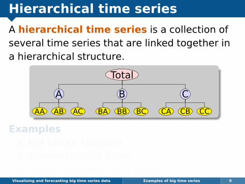
Hierarchical time series
A hierarchical time series is a collection ofseveral time series that are linked together ina hierarchical structure.
Total
A
AA AB AC
B
BA BB BC
C
CA CB CC
ExamplesNet labour turnoverPharmaceutical salesTourism by state and region
Visualising and forecasting big time series data Examples of big time series 9

Grouped time series
A grouped time series is a collection of timeseries that can be grouped together in anumber of non-hierarchical ways.
Total
A
AX AY
B
BX BY
Total
X
AX BX
Y
AY BY
ExamplesTourism by state and purpose of travelGlasses by brand and store
Visualising and forecasting big time series data Examples of big time series 10

Outline
1 Examples of big time series
2 Time series visualisation
3 BLUF: Best Linear Unbiased Forecasts
4 Application: Australian tourism
5 Application: Australian labour market
6 Fast computation tricks
7 hts package for R
8 References
Visualising and forecasting big time series data Time series visualisation 11

Victorian tourism dataB
AA
Hol
BA
BH
ol
BA
AV
isB
AB
Vis
BA
AB
usB
AB
Bus
BA
AO
thB
AB
Oth
BA
CH
olB
BA
Hol
BA
CV
isB
BA
Vis
BA
CB
usB
BA
Bus
BA
CO
thB
BA
Oth
BC
AH
olB
CB
Hol
BC
AV
isB
CB
Vis
BC
AB
usB
CB
Bus
BC
AO
thB
CB
Oth
BC
CH
olB
DA
Hol
BC
CV
isB
DA
Vis
BC
CB
usB
DA
Bus
BC
CO
thB
DA
Oth
BD
BH
olB
DC
Hol
BD
BV
isB
DC
Vis
BD
BB
usB
DC
Bus
BD
BO
thB
DC
Oth
BD
DH
olB
DE
Hol
BD
DV
isB
DE
Vis
BD
DB
usB
DE
Bus
BD
DO
thB
DE
Oth
BD
FH
olB
EA
Hol
BD
FV
isB
EA
Vis
BD
FB
usB
EA
Bus
BD
FO
thB
EA
Oth
BE
BH
olB
EC
Hol
BE
BV
isB
EC
Vis
BE
BB
usB
EC
Bus
BE
BO
thB
EC
Oth
BE
DH
olB
EE
Hol
BE
DV
isB
EE
Vis
BE
DB
usB
EE
Bus
BE
DO
thB
EE
Oth
BE
FH
olB
EG
Hol
BE
FV
isB
EG
Vis
BE
FB
usB
EG
Bus
BE
FO
thB
EG
Oth
Visualising and forecasting big time series data Time series visualisation 12

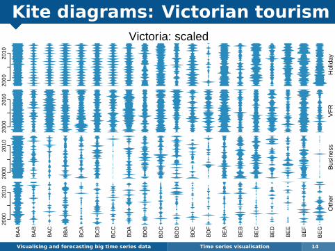
Kite diagrams0
00
Line graph profile
Duplicate & fliparound the hori-zontal axis
Fill the colour
Visualising and forecasting big time series data Time series visualisation 13

Kite diagrams: Victorian tourism20
0020
10
Hol
iday
2000
2010
VF
R
2000
2010
Bus
ines
s
2000
2010
BA
A
BA
B
BA
C
BB
A
BC
A
BC
B
BC
C
BD
A
BD
B
BD
C
BD
D
BD
E
BD
F
BE
A
BE
B
BE
C
BE
D
BE
E
BE
F
Oth
er
BE
G
Victoria
Visualising and forecasting big time series data Time series visualisation 14

Kite diagrams: Victorian tourism
Visualising and forecasting big time series data Time series visualisation 14
Kite diagrams: Victorian tourism20
0020
10
Hol
iday
2000
2010
VF
R
2000
2010
Bus
ines
s
2000
2010
BA
A
BA
B
BA
C
BB
A
BC
A
BC
B
BC
C
BD
A
BD
B
BD
C
BD
D
BD
E
BD
F
BE
A
BE
B
BE
C
BE
D
BE
E
BE
F
Oth
er
BE
G
Victoria: scaled
Visualising and forecasting big time series data Time series visualisation 14

An STL decompositionSTL decomposition of tourism demandfor holidays in Peninsula
5.0
6.0
7.0
data
−0.
50.
5
seas
onal
5.8
6.1
6.4
tren
d
−0.
40.
0
2000 2005 2010
rem
aind
er
timeVisualising and forecasting big time series data Time series visualisation 15

Seasonal stacked bar chart
Place positive values above the originwhile negative values below the originMap the bar length to the magnitudeEncode quarters by colours
Visualising and forecasting big time series data Time series visualisation 16

Seasonal stacked bar chart
Place positive values above the originwhile negative values below the originMap the bar length to the magnitudeEncode quarters by colours
−1.0
−0.5
0.0
0.5
1.0
Holiday
BAA BAB BAC BBABCABCBBCCBDABDBBDCBDDBDEBDF BEA BEBBECBEDBEE BEFBEGRegions
Sea
sona
l Com
pone
nt
Qtr
Q1
Q2
Q3
Q4
Visualising and forecasting big time series data Time series visualisation 16

Seasonal stacked bar chart: VIC
Visualising and forecasting big time series data Time series visualisation 17

Seasonal stacked bar chart: VIC
−1.0−0.5
0.00.51.0
−1.0−0.5
0.00.51.0
−1.0−0.5
0.00.51.0
−1.0−0.5
0.00.51.0
Holiday
VF
RB
usinessO
ther
BAABABBACBBABCABCBBCCBDABDBBDCBDDBDEBDFBEABEBBECBEDBEEBEFBEGRegions
Sea
sona
l Com
pone
nt
QtrQ1Q2Q3Q4
Visualising and forecasting big time series data Time series visualisation 17

Corrgram of remainder
Visualising and forecasting big time series data Time series visualisation 18
Compute the correlationsamong the remaindercomponents
Render both the sign andmagnitude using a colourmapping of two hues
Order variables according tothe first principal component ofthe correlations.

Corrgram of remainder: VIC
Visualising and forecasting big time series data Time series visualisation 19−1
−0.8
−0.6
−0.4
−0.2
0
0.2
0.4
0.6
0.8
1
BE
EH
olB
EF
Oth
BE
EO
thB
DE
Oth
BE
BO
thB
EA
Bus
BE
FB
usB
DC
Oth
BA
CH
olB
EB
Bus
BE
AV
isB
BA
Hol
BD
EH
olB
AB
Oth
BA
AV
isB
AA
Hol
BD
CH
olB
BA
Bus
BC
BH
olB
EG
Bus
BD
DV
isB
AB
Vis
BD
AV
isB
EA
Oth
BD
FH
olB
EE
Bus
BA
AO
thB
AC
Oth
BD
AO
thB
DE
Bus
BC
BO
thB
AC
Bus
BE
BV
isB
AC
Vis
BC
AO
thB
EF
Vis
BC
BV
isB
ED
Hol
BE
GO
thB
DB
Hol
BA
BB
usB
EB
Hol
BD
FB
usB
EC
Hol
BC
AH
olB
DB
Oth
BE
AH
olB
DC
Bus
BE
CV
isB
DB
Vis
BC
CH
olB
BA
Vis
BA
BH
olB
BA
Oth
BC
CO
thB
CB
Bus
BC
CV
isB
EG
Vis
BD
DH
olB
EC
Oth
BD
CV
isB
AA
Bus
BC
CB
usB
EC
Bus
BC
AV
isB
DF
Vis
BE
GH
olB
DD
Oth
BE
DO
thB
ED
Vis
BD
DB
usB
DE
Vis
BE
FH
olB
EE
Vis
BD
BB
usB
DA
Bus
BD
AH
olB
CA
Bus
BD
FO
thB
ED
Bus
BEEHolBEFOthBEEOthBDEOthBEBOthBEABusBEFBusBDCOthBACHolBEBBusBEAVisBBAHolBDEHolBABOthBAAVisBAAHolBDCHolBBABusBCBHolBEGBusBDDVisBABVisBDAVisBEAOthBDFHolBEEBusBAAOthBACOthBDAOthBDEBusBCBOthBACBusBEBVisBACVisBCAOthBEFVisBCBVisBEDHolBEGOthBDBHolBABBusBEBHolBDFBusBECHolBCAHolBDBOthBEAHolBDCBusBECVisBDBVisBCCHolBBAVisBABHolBBAOthBCCOthBCBBusBCCVisBEGVisBDDHolBECOthBDCVisBAABusBCCBusBECBusBCAVisBDFVisBEGHolBDDOthBEDOthBEDVisBDDBusBDEVisBEFHolBEEVisBDBBusBDABusBDAHolBCABusBDFOthBEDBus

Corrgram of remainder: VIC
Visualising and forecasting big time series data Time series visualisation 19−1
−0.8
−0.6
−0.4
−0.2
0
0.2
0.4
0.6
0.8
1
BD
AH
ol
BD
DH
ol
BE
BH
ol
BE
FH
ol
BE
CH
ol
BE
DH
ol
BD
FH
ol
BC
CH
ol
BD
CH
ol
BC
AH
ol
BE
AH
ol
BE
GH
ol
BB
AH
ol
BA
AH
ol
BA
BH
ol
BD
BH
ol
BD
EH
ol
BA
CH
ol
BC
BH
ol
BE
EH
ol
BDAHol
BDDHol
BEBHol
BEFHol
BECHol
BEDHol
BDFHol
BCCHol
BDCHol
BCAHol
BEAHol
BEGHol
BBAHol
BAAHol
BABHol
BDBHol
BDEHol
BACHol
BCBHol
BEEHol

Corrgram of remainder: TAS
Visualising and forecasting big time series data Time series visualisation 20−1
−0.8
−0.6
−0.4
−0.2
0
0.2
0.4
0.6
0.8
1
FC
AH
ol
FB
BH
ol
FB
AH
ol
FAA
Hol
FC
BH
ol
FC
AV
is
FB
BV
is
FAA
Vis
FC
BB
us
FAA
Oth
FC
AO
th
FB
BO
th
FB
AB
us
FB
AO
th
FC
BV
is
FC
AB
us
FB
AV
is
FC
BO
th
FB
BB
us
FAA
Bus
FCAHol
FBBHol
FBAHol
FAAHol
FCBHol
FCAVis
FBBVis
FAAVis
FCBBus
FAAOth
FCAOth
FBBOth
FBABus
FBAOth
FCBVis
FCABus
FBAVis
FCBOth
FBBBus
FAABus
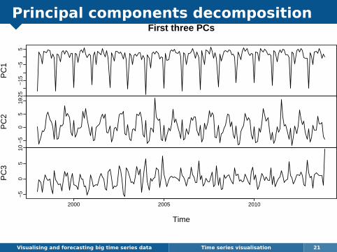
Principal components decomposition
Visualising and forecasting big time series data Time series visualisation 21
−25
−15
−5
5
PC
1
−5
05
10
PC
2
−5
05
10
2000 2005 2010
PC
3
Time
First three PCs

Principal components decomposition
Visualising and forecasting big time series data Time series visualisation 21
−25
−20
−15
−10
−5
05
Season plot: PC1
Month
Jan Feb Mar Apr May Jun Jul Aug Sep Oct Nov Dec

Principal components decomposition
Visualising and forecasting big time series data Time series visualisation 21
−5
05
10
Season plot: PC2
Month
Jan Feb Mar Apr May Jun Jul Aug Sep Oct Nov Dec
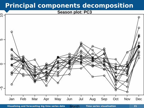
Principal components decomposition
Visualising and forecasting big time series data Time series visualisation 21
−5
05
10
Season plot: PC3
Month
Jan Feb Mar Apr May Jun Jul Aug Sep Oct Nov Dec

Principal components decomposition
Visualising and forecasting big time series data Time series visualisation 22
−0.15 −0.10 −0.05 0.00 0.05
−0.
100.
000.
050.
100.
150.
20
Loading 1
Load
ing
2
NSWVICQLDSATASNTWA

Principal components decomposition
Visualising and forecasting big time series data Time series visualisation 22
−0.15 −0.10 −0.05 0.00 0.05
−0.
100.
000.
050.
100.
150.
20
Loading 1
Load
ing
2
HolVisBusOth
Feature analysis
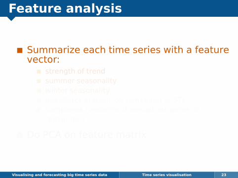
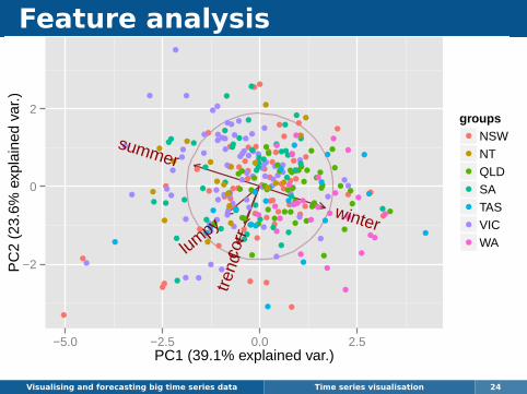
Summarize each time series with a featurevector:
strength of trendsummer seasonalitywinter seasonalityBox-Pierce statistic on remainder of STLLumpiness (variance of annual variances ofremainder)
Do PCA on feature matrix
Visualising and forecasting big time series data Time series visualisation 23

Feature analysis
Visualising and forecasting big time series data Time series visualisation 24
trend
summer
winterco
rrlumpy
−2
0
2
−5.0 −2.5 0.0 2.5PC1 (39.1% explained var.)
PC
2 (2
3.6%
exp
lain
ed v
ar.)
groups
BusHolOthVis
Feature analysis
Visualising and forecasting big time series data Time series visualisation 24
trend
summer
winterco
rrlumpy
−2
0
2
−5.0 −2.5 0.0 2.5PC1 (39.1% explained var.)
PC
2 (2
3.6%
exp
lain
ed v
ar.)
groups
NSWNTQLDSATASVICWA

Outline
1 Examples of big time series
2 Time series visualisation
3 BLUF: Best Linear Unbiased Forecasts
4 Application: Australian tourism
5 Application: Australian labour market
6 Fast computation tricks
7 hts package for R
8 References
Visualising and forecasting big time series data BLUF: Best Linear Unbiased Forecasts 25

Hierarchical/grouped time seriesForecasts should be “aggregateconsistent”, unbiased, minimum variance.
Existing methods:ã Bottom-upã Top-downã Middle-out
How to compute forecast intervals?
Most research is concerned about relativeperformance of existing methods.
Visualising and forecasting big time series data BLUF: Best Linear Unbiased Forecasts 26

Top-down method
Visualising and forecasting big time series data BLUF: Best Linear Unbiased Forecasts 27
Advantages
Works well inpresence of lowcounts.
Single forecastingmodel easy tobuild
Provides reliableforecasts foraggregate levels.
Disadvantages
Loss of information,especiallyindividual seriesdynamics.
Distribution offorecasts to lowerlevels can bedifficult
No predictionintervals
Bottom-up method
Visualising and forecasting big time series data BLUF: Best Linear Unbiased Forecasts 28
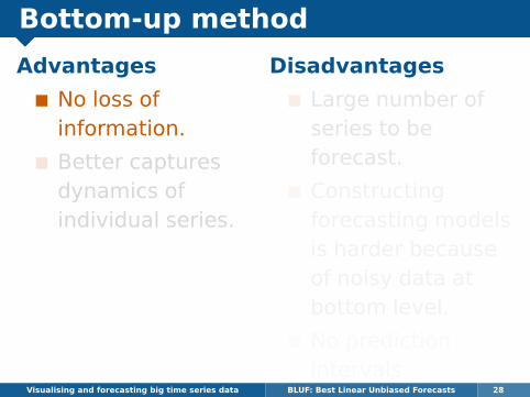
Advantages
No loss ofinformation.
Better capturesdynamics ofindividual series.
Disadvantages
Large number ofseries to beforecast.
Constructingforecasting modelsis harder becauseof noisy data atbottom level.
No predictionintervals

Bottom-up method
Visualising and forecasting big time series data BLUF: Best Linear Unbiased Forecasts 28
Advantages
No loss ofinformation.
Better capturesdynamics ofindividual series.
Disadvantages
Large number ofseries to beforecast.
Constructingforecasting modelsis harder becauseof noisy data atbottom level.
No predictionintervals

The BLUF approach
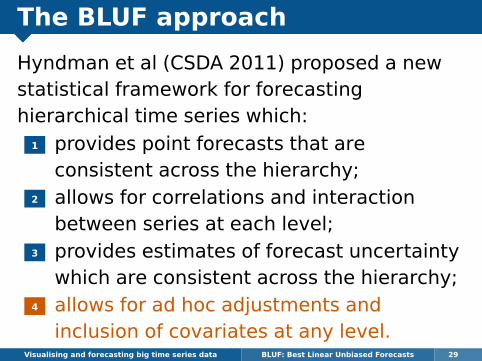
Hyndman et al (CSDA 2011) proposed a newstatistical framework for forecastinghierarchical time series which:
1 provides point forecasts that areconsistent across the hierarchy;
2 allows for correlations and interactionbetween series at each level;
3 provides estimates of forecast uncertaintywhich are consistent across the hierarchy;
4 allows for ad hoc adjustments andinclusion of covariates at any level.
Visualising and forecasting big time series data BLUF: Best Linear Unbiased Forecasts 29

The BLUF approach
Hyndman et al (CSDA 2011) proposed a newstatistical framework for forecastinghierarchical time series which:
1 provides point forecasts that areconsistent across the hierarchy;
2 allows for correlations and interactionbetween series at each level;
3 provides estimates of forecast uncertaintywhich are consistent across the hierarchy;
4 allows for ad hoc adjustments andinclusion of covariates at any level.
Visualising and forecasting big time series data BLUF: Best Linear Unbiased Forecasts 29

Hierarchical data
Total
A B C
Visualising and forecasting big time series data BLUF: Best Linear Unbiased Forecasts 30
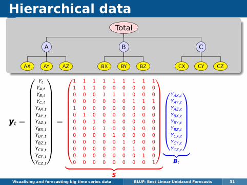
Yt : observed aggregate of allseries at time t.
YX,t : observation on series X attime t.
Bt : vector of all series atbottom level in time t.

Hierarchical data
Total
A B C
Visualising and forecasting big time series data BLUF: Best Linear Unbiased Forecasts 30
Yt : observed aggregate of allseries at time t.
YX,t : observation on series X attime t.
Bt : vector of all series atbottom level in time t.

Hierarchical data
Total
A B C
yt = [Yt, YA,t, YB,t, YC,t]′ =
1 1 11 0 00 1 00 0 1
YA,tYB,tYC,t
Visualising and forecasting big time series data BLUF: Best Linear Unbiased Forecasts 30
Yt : observed aggregate of allseries at time t.
YX,t : observation on series X attime t.
Bt : vector of all series atbottom level in time t.

Hierarchical data
Total
A B C
yt = [Yt, YA,t, YB,t, YC,t]′ =
1 1 11 0 00 1 00 0 1
︸ ︷︷ ︸
S
YA,tYB,tYC,t
︸ ︷︷ ︸
Bt
Visualising and forecasting big time series data BLUF: Best Linear Unbiased Forecasts 30
Yt : observed aggregate of allseries at time t.
YX,t : observation on series X attime t.
Bt : vector of all series atbottom level in time t.

Hierarchical data
Total
A B C
yt = [Yt, YA,t, YB,t, YC,t]′ =
1 1 11 0 00 1 00 0 1
︸ ︷︷ ︸
S
YA,tYB,tYC,t
︸ ︷︷ ︸
Btyt = SBt
Visualising and forecasting big time series data BLUF: Best Linear Unbiased Forecasts 30
Yt : observed aggregate of allseries at time t.
YX,t : observation on series X attime t.
Bt : vector of all series atbottom level in time t.

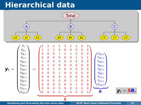
Hierarchical dataTotal
A
AX AY AZ
B
BX BY BZ
C
CX CY CZ
yt =
YtYA,tYB,tYC,tYAX,tYAY,tYAZ,tYBX,tYBY,tYBZ,tYCX,tYCY,tYCZ,t
=
1 1 1 1 1 1 1 1 11 1 1 0 0 0 0 0 00 0 0 1 1 1 0 0 00 0 0 0 0 0 1 1 11 0 0 0 0 0 0 0 00 1 0 0 0 0 0 0 00 0 1 0 0 0 0 0 00 0 0 1 0 0 0 0 00 0 0 0 1 0 0 0 00 0 0 0 0 1 0 0 00 0 0 0 0 0 1 0 00 0 0 0 0 0 0 1 00 0 0 0 0 0 0 0 1
︸ ︷︷ ︸
S
YAX,tYAY,tYAZ,tYBX,tYBY,tYBZ,tYCX,tYCY,tYCZ,t
︸ ︷︷ ︸
Bt
Visualising and forecasting big time series data BLUF: Best Linear Unbiased Forecasts 31
yt = SBt

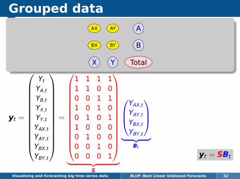
Grouped dataAX AY A
BX BY B
X Y Total
yt =
YtYA,tYB,tYX,tYY,tYAX,tYAY,tYBX,tYBY,t
=
1 1 1 11 1 0 00 0 1 11 0 1 00 1 0 11 0 0 00 1 0 00 0 1 00 0 0 1
︸ ︷︷ ︸
S
YAX,tYAY,tYBX,tYBY,t
︸ ︷︷ ︸
Bt
Visualising and forecasting big time series data BLUF: Best Linear Unbiased Forecasts 32

Grouped dataAX AY A
BX BY B
X Y Total
yt =
YtYA,tYB,tYX,tYY,tYAX,tYAY,tYBX,tYBY,t
=
1 1 1 11 1 0 00 0 1 11 0 1 00 1 0 11 0 0 00 1 0 00 0 1 00 0 0 1
︸ ︷︷ ︸
S
YAX,tYAY,tYBX,tYBY,t
︸ ︷︷ ︸
Bt
Visualising and forecasting big time series data BLUF: Best Linear Unbiased Forecasts 32
Grouped dataAX AY A
BX BY B
X Y Total
yt =
YtYA,tYB,tYX,tYY,tYAX,tYAY,tYBX,tYBY,t
=
1 1 1 11 1 0 00 0 1 11 0 1 00 1 0 11 0 0 00 1 0 00 0 1 00 0 0 1
︸ ︷︷ ︸
S
YAX,tYAY,tYBX,tYBY,t
︸ ︷︷ ︸
Bt
Visualising and forecasting big time series data BLUF: Best Linear Unbiased Forecasts 32
yt = SBt

Forecasting notation
Let yn(h) be vector of initial h-step forecasts,made at time n, stacked in same order as yt.(They may not add up.)
Hierarchical forecasting methods of the form:yn(h) = SPyn(h)
for some matrix P.
P extracts and combines base forecastsyn(h) to get bottom-level forecasts.S adds them upRevised reconciled forecasts: yn(h).
Visualising and forecasting big time series data BLUF: Best Linear Unbiased Forecasts 33

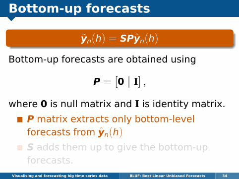
Bottom-up forecasts
yn(h) = SPyn(h)
Bottom-up forecasts are obtained using
P = [0 | I] ,
where 0 is null matrix and I is identity matrix.
P matrix extracts only bottom-levelforecasts from yn(h)
S adds them up to give the bottom-upforecasts.
Visualising and forecasting big time series data BLUF: Best Linear Unbiased Forecasts 34

Top-down forecasts
yn(h) = SPyn(h)
Top-down forecasts are obtained using
P = [p | 0]
where p = [p1, p2, . . . , pmK]′ is a vector of
proportions that sum to one.
P distributes forecasts of the aggregate tothe lowest level series.
Different methods of top-down forecastinglead to different proportionality vectors p.
Visualising and forecasting big time series data BLUF: Best Linear Unbiased Forecasts 35

General properties: bias
yn(h) = SPyn(h)
Assume: base forecasts yn(h) are unbiased:E[yn(h)|y1, . . . ,yn] = E[yn+h|y1, . . . ,yn]
Let Bn(h) be bottom level base forecastswith βn(h) = E[Bn(h)|y1, . . . ,yn].Then E[yn(h)] = Sβn(h).We want the revised forecasts to be unbiased:E[yn(h)] = SPSβn(h) = Sβn(h).Result will hold provided SPS = S.True for bottom-up, but not for any top-downmethod or middle-out method.
Visualising and forecasting big time series data BLUF: Best Linear Unbiased Forecasts 36

General properties: variance
yn(h) = SPyn(h)
Let variance of base forecasts yn(h) be givenby
Σh = Var[yn(h)|y1, . . . , yn]
Then the variance of the revised forecasts isgiven by
Var[yn(h)|y1, . . . , yn] = SPΣhP′S′.
This is a general result for all existing methods.Visualising and forecasting big time series data BLUF: Best Linear Unbiased Forecasts 37
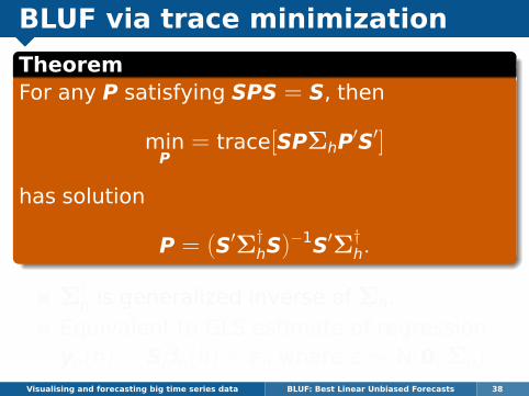
BLUF via trace minimization
TheoremFor any P satisfying SPS = S, then
minP
= trace[SPΣhP′S′]
has solution
P = (S′Σ†hS)−1S′Σ†h.
Σ†h is generalized inverse of Σh.
Equivalent to GLS estimate of regressionyn(h) = Sβn(h) + εh where ε ∼ N(0,Σh).
Visualising and forecasting big time series data BLUF: Best Linear Unbiased Forecasts 38

Optimal combination forecasts
yn(h) = SPyn(h) = S(S′Σ†hS)−1S′Σ†hyn(h)
Σ†h is generalized inverse of Σh.
Var[yn(h)|y1, . . . , yn] = S(S′Σ†hS)−1S′
Problem: Σh hard to estimate.
Visualising and forecasting big time series data BLUF: Best Linear Unbiased Forecasts 39

Optimal combination forecasts
yn(h) = SPyn(h) = S(S′Σ†hS)−1S′Σ†hyn(h)
Initial forecasts
Σ†h is generalized inverse of Σh.
Var[yn(h)|y1, . . . , yn] = S(S′Σ†hS)−1S′
Problem: Σh hard to estimate.
Visualising and forecasting big time series data BLUF: Best Linear Unbiased Forecasts 39

Optimal combination forecasts
yn(h) = SPyn(h) = S(S′Σ†hS)−1S′Σ†hyn(h)
Revised forecasts Initial forecasts
Σ†h is generalized inverse of Σh.
Var[yn(h)|y1, . . . , yn] = S(S′Σ†hS)−1S′
Problem: Σh hard to estimate.
Visualising and forecasting big time series data BLUF: Best Linear Unbiased Forecasts 39

Optimal combination forecasts
yn(h) = S(S′Σ†hS)−1S′Σ†hyn(h)
Revised forecasts Base forecasts
Solution 1: OLSAssume εh ≈ SεB,h where εB,h is theforecast error at bottom level.
Then Σh ≈ SΩhS′ where Ωh = Var(εB,h).
If Moore-Penrose generalized inverse used,then (S′Σ†hS)
−1S′Σ†h = (S′S)−1S′.
yn(h) = S(S′S)−1S′yn(h)Visualising and forecasting big time series data BLUF: Best Linear Unbiased Forecasts 40

Optimal combination forecasts
Visualising and forecasting big time series data BLUF: Best Linear Unbiased Forecasts 41
yn(h) = S(S′S)−1S′yn(h)Total
A B C

Optimal combination forecasts
Visualising and forecasting big time series data BLUF: Best Linear Unbiased Forecasts 41
yn(h) = S(S′S)−1S′yn(h)Total
A B C
Weights:
S(S′S)−1S′ =
0.75 0.25 0.25 0.250.25 0.75 −0.25 −0.250.25 −0.25 0.75 −0.250.25 −0.25 −0.25 0.75

Optimal combination forecasts
Total
A
AA AB AC
B
BA BB BC
C
CA CB CC
Weights: S(S′S)−1S′ =
0.69 0.23 0.23 0.23 0.08 0.08 0.08 0.08 0.08 0.08 0.08 0.08 0.080.23 0.58 −0.17 −0.17 0.19 0.19 0.19 −0.06 −0.06 −0.06 −0.06 −0.06 −0.060.23 −0.17 0.58 −0.17 −0.06 −0.06 −0.06 0.19 0.19 0.19 −0.06 −0.06 −0.060.23 −0.17 −0.17 0.58 −0.06 −0.06 −0.06 −0.06 −0.06 −0.06 0.19 0.19 0.190.08 0.19 −0.06 −0.06 0.73 −0.27 −0.27 −0.02 −0.02 −0.02 −0.02 −0.02 −0.020.08 0.19 −0.06 −0.06 −0.27 0.73 −0.27 −0.02 −0.02 −0.02 −0.02 −0.02 −0.020.08 0.19 −0.06 −0.06 −0.27 −0.27 0.73 −0.02 −0.02 −0.02 −0.02 −0.02 −0.020.08 −0.06 0.19 −0.06 −0.02 −0.02 −0.02 0.73 −0.27 −0.27 −0.02 −0.02 −0.020.08 −0.06 0.19 −0.06 −0.02 −0.02 −0.02 −0.27 0.73 −0.27 −0.02 −0.02 −0.020.08 −0.06 0.19 −0.06 −0.02 −0.02 −0.02 −0.27 −0.27 0.73 −0.02 −0.02 −0.020.08 −0.06 −0.06 0.19 −0.02 −0.02 −0.02 −0.02 −0.02 −0.02 0.73 −0.27 −0.270.08 −0.06 −0.06 0.19 −0.02 −0.02 −0.02 −0.02 −0.02 −0.02 −0.27 0.73 −0.270.08 −0.06 −0.06 0.19 −0.02 −0.02 −0.02 −0.02 −0.02 −0.02 −0.27 −0.27 0.73
Visualising and forecasting big time series data BLUF: Best Linear Unbiased Forecasts 42

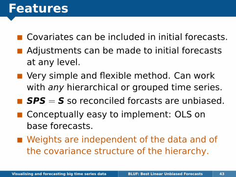
Features
Covariates can be included in initial forecasts.
Adjustments can be made to initial forecastsat any level.
Very simple and flexible method. Can workwith any hierarchical or grouped time series.
SPS = S so reconciled forcasts are unbiased.
Conceptually easy to implement: OLS onbase forecasts.
Weights are independent of the data and ofthe covariance structure of the hierarchy.
Visualising and forecasting big time series data BLUF: Best Linear Unbiased Forecasts 43

Challenges
Computational difficulties in bighierarchies due to size of the S matrix andsingular behavior of (S′S).
Need to estimate covariance matrix toproduce prediction intervals.
Ignores covariance matrix in computingpoint forecasts.
Visualising and forecasting big time series data BLUF: Best Linear Unbiased Forecasts 44
yn(h) = S(S′S)−1S′yn(h)

Optimal combination forecasts
Solution 1: OLSApproximate Σ†1 by cI.
Solution 2: RescalingSuppose we approximate Σ1 by itsdiagonal.
Let Λ =[diagonal
(Σ1
)]−1contain inverse
one-step forecast variances.
Visualising and forecasting big time series data BLUF: Best Linear Unbiased Forecasts 45
yn(h) = S(S′Σ†1S)−1S′Σ†1yn(h)
yn(h) = S(S′ΛS)−1S′Λyn(h)

Optimal reconciled forecasts
yn(h) = Sβn(h) = S(S′ΛS)−1S′Λyn(h)
Easy to estimate, and places weight wherewe have best forecasts.Ignores covariances.For large numbers of time series, we needto do calculation without explicitly formingS or (S′ΛS)−1 or S′Λ.
Visualising and forecasting big time series data BLUF: Best Linear Unbiased Forecasts 46

Optimal reconciled forecasts
yn(h) = Sβn(h) = S(S′ΛS)−1S′Λyn(h)
Initial forecasts
Easy to estimate, and places weight wherewe have best forecasts.Ignores covariances.For large numbers of time series, we needto do calculation without explicitly formingS or (S′ΛS)−1 or S′Λ.
Visualising and forecasting big time series data BLUF: Best Linear Unbiased Forecasts 46

Optimal reconciled forecasts
yn(h) = Sβn(h) = S(S′ΛS)−1S′Λyn(h)
Revised forecasts Initial forecasts
Easy to estimate, and places weight wherewe have best forecasts.Ignores covariances.For large numbers of time series, we needto do calculation without explicitly formingS or (S′ΛS)−1 or S′Λ.
Visualising and forecasting big time series data BLUF: Best Linear Unbiased Forecasts 46

Outline
1 Examples of big time series
2 Time series visualisation
3 BLUF: Best Linear Unbiased Forecasts
4 Application: Australian tourism
5 Application: Australian labour market
6 Fast computation tricks
7 hts package for R
8 References
Visualising and forecasting big time series data Application: Australian tourism 47

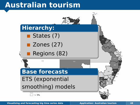
Australian tourism
Visualising and forecasting big time series data Application: Australian tourism 48

Australian tourism
Visualising and forecasting big time series data Application: Australian tourism 48
Hierarchy:States (7)
Zones (27)
Regions (82)
Australian tourism
Visualising and forecasting big time series data Application: Australian tourism 48
Hierarchy:States (7)
Zones (27)
Regions (82)
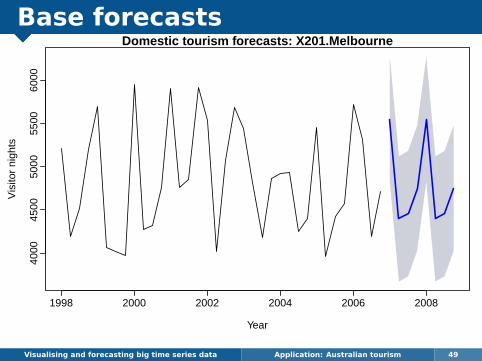
Base forecastsETS (exponentialsmoothing) models

Base forecasts
Visualising and forecasting big time series data Application: Australian tourism 49
Domestic tourism forecasts: Total
Year
Vis
itor
nigh
ts
1998 2000 2002 2004 2006 2008
6000
065
000
7000
075
000
8000
085
000
Base forecasts
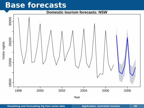
Visualising and forecasting big time series data Application: Australian tourism 49
Domestic tourism forecasts: NSW
Year
Vis
itor
nigh
ts
1998 2000 2002 2004 2006 2008
1800
022
000
2600
030
000

Base forecasts
Visualising and forecasting big time series data Application: Australian tourism 49
Domestic tourism forecasts: VIC
Year
Vis
itor
nigh
ts
1998 2000 2002 2004 2006 2008
1000
012
000
1400
016
000
1800
0

Base forecasts
Visualising and forecasting big time series data Application: Australian tourism 49
Domestic tourism forecasts: Nth.Coast.NSW
Year
Vis
itor
nigh
ts
1998 2000 2002 2004 2006 2008
5000
6000
7000
8000
9000

Base forecasts
Visualising and forecasting big time series data Application: Australian tourism 49
Domestic tourism forecasts: Metro.QLD
Year
Vis
itor
nigh
ts
1998 2000 2002 2004 2006 2008
8000
9000
1100
013
000

Base forecasts
Visualising and forecasting big time series data Application: Australian tourism 49
Domestic tourism forecasts: Sth.WA
Year
Vis
itor
nigh
ts
1998 2000 2002 2004 2006 2008
400
600
800
1000
1200
1400
Base forecasts
Visualising and forecasting big time series data Application: Australian tourism 49
Domestic tourism forecasts: X201.Melbourne
Year
Vis
itor
nigh
ts
1998 2000 2002 2004 2006 2008
4000
4500
5000
5500
6000

Base forecasts
Visualising and forecasting big time series data Application: Australian tourism 49
Domestic tourism forecasts: X402.Murraylands
Year
Vis
itor
nigh
ts
1998 2000 2002 2004 2006 2008
010
020
030
0

Base forecasts
Visualising and forecasting big time series data Application: Australian tourism 49
Domestic tourism forecasts: X809.Daly
Year
Vis
itor
nigh
ts
1998 2000 2002 2004 2006 2008
020
4060
8010
0

Reconciled forecasts
Visualising and forecasting big time series data Application: Australian tourism 50
Tota
l
2000 2005 2010
6500
080
000
9500
0
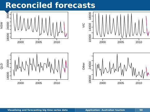
Reconciled forecasts
Visualising and forecasting big time series data Application: Australian tourism 50
NS
W
2000 2005 2010
1800
024
000
3000
0
VIC
2000 2005 20101000
014
000
1800
0
QLD
2000 2005 2010
1400
020
000
Oth
er2000 2005 201018
000
2400
0

Reconciled forecasts
Visualising and forecasting big time series data Application: Australian tourism 50
Syd
ney
2000 2005 20104000
7000
Oth
er N
SW
2000 2005 2010
1400
022
000
Mel
bour
ne
2000 2005 2010
4000
5000
Oth
er V
IC
2000 2005 2010
6000
1200
0
GC
and
Bris
bane
2000 2005 2010
6000
9000
Oth
er Q
LD2000 2005 201060
0012
000
Cap
ital c
ities
2000 2005 2010
1400
020
000
Oth
er
2000 2005 2010
5500
7500

Forecast evaluation
Select models using all observations;
Re-estimate models using first 12observations and generate 1- to8-step-ahead forecasts;
Increase sample size one observation at atime, re-estimate models, generateforecasts until the end of the sample;
In total 24 1-step-ahead, 232-steps-ahead, up to 17 8-steps-ahead forforecast evaluation.
Visualising and forecasting big time series data Application: Australian tourism 51

Hierarchy: states, zones, regions
MAPE h = 1 h = 2 h = 4 h = 6 h = 8 AverageTop Level: Australia
Bottom-up 3.79 3.58 4.01 4.55 4.24 4.06OLS 3.83 3.66 3.88 4.19 4.25 3.94Scaling (st. dev.) 3.68 3.56 3.97 4.57 4.25 4.04Level: States
Bottom-up 10.70 10.52 10.85 11.46 11.27 11.03OLS 11.07 10.58 11.13 11.62 12.21 11.35Scaling (st. dev.) 10.44 10.17 10.47 10.97 10.98 10.67Level: Zones
Bottom-up 14.99 14.97 14.98 15.69 15.65 15.32OLS 15.16 15.06 15.27 15.74 16.15 15.48Scaling (st. dev.) 14.63 14.62 14.68 15.17 15.25 14.94Bottom Level: Regions
Bottom-up 33.12 32.54 32.26 33.74 33.96 33.18OLS 35.89 33.86 34.26 36.06 37.49 35.43Scaling (st. dev.) 31.68 31.22 31.08 32.41 32.77 31.89
Visualising and forecasting big time series data Application: Australian tourism 52
Outline
1 Examples of big time series
2 Time series visualisation
3 BLUF: Best Linear Unbiased Forecasts
4 Application: Australian tourism
5 Application: Australian labour market
6 Fast computation tricks
7 hts package for R
8 References
Visualising and forecasting big time series data Application: Australian labour market 53

ANZSCO
Australia and New Zealand StandardClassification of Occupations
8 major groups43 sub-major groups
97 minor groups– 359 unit groups
* 1023 occupations
Example: statistician2 Professionals
22 Business, Human Resource and MarketingProfessionals224 Information and Organisation Professionals
2241 Actuaries, Mathematicians and Statisticians224113 Statistician
Visualising and forecasting big time series data Application: Australian labour market 54

Australian Labour Market data
Visualising and forecasting big time series data Application: Australian labour market 55
Time
Leve
l 0
7000
9000
1100
0
Time
Leve
l 1
500
1000
1500
2000
2500
1. Managers2. Professionals3. Technicians and trade workers4. Community and personal services workers5. Clerical and administrative workers6. Sales workers7. Machinery operators and drivers8. Labourers
Time
Leve
l 2
100
200
300
400
500
600
700
Time
Leve
l 3
100
200
300
400
500
600
700
Time
Leve
l 4
1990 1995 2000 2005 2010
100
200
300
400
500
Lower three panelsshow largestsub-groups at eachlevel.

Australian Labour Market data
Visualising and forecasting big time series data Application: Australian labour market 55
Time
Leve
l 0
7000
9000
1100
0
Time
Leve
l 1
500
1000
1500
2000
2500
1. Managers2. Professionals3. Technicians and trade workers4. Community and personal services workers5. Clerical and administrative workers6. Sales workers7. Machinery operators and drivers8. Labourers
Time
Leve
l 2
100
200
300
400
500
600
700
Time
Leve
l 3
100
200
300
400
500
600
700
Time
Leve
l 4
1990 1995 2000 2005 2010
100
200
300
400
500
Time
Leve
l 0
1080
011
200
1160
012
000
Base forecastsReconciled forecasts
Time
Leve
l 1
680
700
720
740
760
780
800
Time
Leve
l 2
140
150
160
170
180
190
200
Time
Leve
l 3
140
150
160
170
180
Year
Leve
l 4
2010 2011 2012 2013 2014 2015
120
130
140
150
160
Base forecastsfrom auto.arima()
Largest changesshown for eachlevel
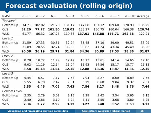
Forecast evaluation (rolling origin)RMSE h = 1 h = 2 h = 3 h = 4 h = 5 h = 6 h = 7 h = 8 Average
Top level
Bottom-up 74.71 102.02 121.70 131.17 147.08 157.12 169.60 178.93 135.29
OLS 52.20 77.77 101.50 119.03 138.27 150.75 160.04 166.38 120.74
WLS 61.77 86.32 107.26 119.33 137.01 146.88 156.71 162.38 122.21
Level 1
Bottom-up 21.59 27.33 30.81 32.94 35.45 37.10 39.00 40.51 33.09
OLS 21.89 28.55 32.74 35.58 38.82 41.24 43.34 45.49 35.96
WLS 20.58 26.19 29.71 31.84 34.36 35.89 37.53 38.86 31.87
Level 2
Bottom-up 8.78 10.72 11.79 12.42 13.13 13.61 14.14 14.65 12.40
OLS 9.02 11.19 12.34 13.04 13.92 14.56 15.17 15.77 13.13
WLS 8.58 10.48 11.54 12.15 12.88 13.36 13.87 14.36 12.15
Level 3
Bottom-up 5.44 6.57 7.17 7.53 7.94 8.27 8.60 8.89 7.55
OLS 5.55 6.78 7.42 7.81 8.29 8.68 9.04 9.37 7.87
WLS 5.35 6.46 7.06 7.42 7.84 8.17 8.48 8.76 7.44
Bottom Level
Bottom-up 2.35 2.79 3.02 3.15 3.29 3.42 3.54 3.65 3.15
OLS 2.40 2.86 3.10 3.24 3.41 3.55 3.68 3.80 3.25
WLS 2.34 2.77 2.99 3.12 3.27 3.40 3.52 3.63 3.13
Visualising and forecasting big time series data Application: Australian labour market 56

Outline
1 Examples of big time series
2 Time series visualisation
3 BLUF: Best Linear Unbiased Forecasts
4 Application: Australian tourism
5 Application: Australian labour market
6 Fast computation tricks
7 hts package for R
8 References
Visualising and forecasting big time series data Fast computation tricks 57

Fast computation: hierarchical data
Total
A
AX AY AZ
B
BX BY BZ
C
CX CY CZ
yt =
YtYA,tYB,tYC,tYAX,tYAY,tYAZ,tYBX,tYBY,tYBZ,tYCX,tYCY,tYCZ,t
=
1 1 1 1 1 1 1 1 11 1 1 0 0 0 0 0 00 0 0 1 1 1 0 0 00 0 0 0 0 0 1 1 11 0 0 0 0 0 0 0 00 1 0 0 0 0 0 0 00 0 1 0 0 0 0 0 00 0 0 1 0 0 0 0 00 0 0 0 1 0 0 0 00 0 0 0 0 1 0 0 00 0 0 0 0 0 1 0 00 0 0 0 0 0 0 1 00 0 0 0 0 0 0 0 1
︸ ︷︷ ︸
S
YAX,tYAY,tYAZ,tYBX,tYBY,tYBZ,tYCX,tYCY,tYCZ,t
︸ ︷︷ ︸
Bt
Visualising and forecasting big time series data Fast computation tricks 58
yt = SBt

Fast computation: hierarchical data
Total
A
AX AY AZ
B
BX BY BZ
C
CX CY CZ
yt =
YtYA,tYAX,tYAY,tYAZ,tYB,tYBX,tYBY,tYBZ,tYC,tYCX,tYCY,tYCZ,t
=
1 1 1 1 1 1 1 1 11 1 1 0 0 0 0 0 01 0 0 0 0 0 0 0 00 1 0 0 0 0 0 0 00 0 1 0 0 0 0 0 00 0 0 1 1 1 0 0 00 0 0 1 0 0 0 0 00 0 0 0 1 0 0 0 00 0 0 0 0 1 0 0 00 0 0 0 0 0 1 1 10 0 0 0 0 0 1 0 00 0 0 0 0 0 0 1 00 0 0 0 0 0 0 0 1
︸ ︷︷ ︸
S
YAX,tYAY,tYAZ,tYBX,tYBY,tYBZ,tYCX,tYCY,tYCZ,t
︸ ︷︷ ︸
Bt
Visualising and forecasting big time series data Fast computation tricks 59
yt = SBt

Fast computation: hierarchies
Think of the hierarchy as a tree of trees:
Total
T1 T2 . . . TK
Then the summing matrix contains k smaller summingmatrices:
S =
1′n1
1′n2· · · 1′nK
S1 0 · · · 00 S2 · · · 0...
... . . . ...0 0 · · · SK
where 1n is an n-vector of ones and tree Ti has niterminal nodes.
Visualising and forecasting big time series data Fast computation tricks 60

Fast computation: hierarchies
S′ΛS =
S′1Λ1S1 0 · · · 0
0 S′2Λ2S2 · · · 0... ... . . . ...0 0 · · · S′KΛKSK
+λ0 Jn
λ0 is the top left element of Λ;Λk is a block of Λ, corresponding to tree Tk;Jn is a matrix of ones;n =
∑k nk.
Now apply the Sherman-Morrison formula . . .
Visualising and forecasting big time series data Fast computation tricks 61

Fast computation: hierarchies
(S′ΛS)−1 =
(S′1Λ1S1)
−1 0 · · · 00 (S′2Λ2S2)
−1 · · · 0...
.... . .
...0 0 · · · (S′KΛKSK)
−1
−cS0
S0 can be partitioned into K2 blocks, with the (k, `)block (of dimension nk × n`) being
(S′kΛkSk)−1Jnk,n`(S
′`Λ`S`)
−1
Jnk,n` is a nk × n` matrix of ones.
c−1 = λ−10 +
∑k
1′nk(S′kΛkSk)
−11nk .
Each S′kΛkSk can be inverted similarly.S′Λy can also be computed recursively.
Visualising and forecasting big time series data Fast computation tricks 62
The recursive calculations can bedone in such a way that we neverstore any of the large matricesinvolved.

Fast computation
When the time series are not strictlyhierarchical and have more than two groupingvariables:
Use sparse matrix storage and arithmetic.
Use iterative approximation for invertinglarge sparse matrices.
Paige & Saunders (1982)ACM Trans. Math. Software
Visualising and forecasting big time series data Fast computation tricks 63

Outline
1 Examples of big time series
2 Time series visualisation
3 BLUF: Best Linear Unbiased Forecasts
4 Application: Australian tourism
5 Application: Australian labour market
6 Fast computation tricks
7 hts package for R
8 References
Visualising and forecasting big time series data hts package for R 64

hts package for R
Visualising and forecasting big time series data hts package for R 65
hts: Hierarchical and grouped time seriesMethods for analysing and forecasting hierarchical and groupedtime series
Version: 4.3Depends: forecast (≥ 5.0)Imports: SparseM, parallel, utilsPublished: 2014-06-10Author: Rob J Hyndman, Earo Wang and Alan LeeMaintainer: Rob J Hyndman <Rob.Hyndman at monash.edu>BugReports: https://github.com/robjhyndman/hts/issuesLicense: GPL (≥ 2)

Example using Rlibrary(hts)
# bts is a matrix containing the bottom level time series# nodes describes the hierarchical structurey <- hts(bts, nodes=list(2, c(3,2)))
Visualising and forecasting big time series data hts package for R 66

Example using Rlibrary(hts)
# bts is a matrix containing the bottom level time series# nodes describes the hierarchical structurey <- hts(bts, nodes=list(2, c(3,2)))
Visualising and forecasting big time series data hts package for R 66
Total
A
AX AY AZ
B
BX BY

Example using Rlibrary(hts)
# bts is a matrix containing the bottom level time series# nodes describes the hierarchical structurey <- hts(bts, nodes=list(2, c(3,2)))
# Forecast 10-step-ahead using WLS combination method# ETS used for each series by defaultfc <- forecast(y, h=10)
Visualising and forecasting big time series data hts package for R 67
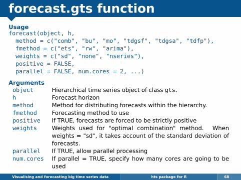
forecast.gts functionUsageforecast(object, h,method = c("comb", "bu", "mo", "tdgsf", "tdgsa", "tdfp"),fmethod = c("ets", "rw", "arima"),weights = c("sd", "none", "nseries"),positive = FALSE,parallel = FALSE, num.cores = 2, ...)
Argumentsobject Hierarchical time series object of class gts.h Forecast horizonmethod Method for distributing forecasts within the hierarchy.fmethod Forecasting method to usepositive If TRUE, forecasts are forced to be strictly positiveweights Weights used for "optimal combination" method. When
weights = "sd", it takes account of the standard deviation offorecasts.
parallel If TRUE, allow parallel processingnum.cores If parallel = TRUE, specify how many cores are going to be
used
Visualising and forecasting big time series data hts package for R 68
Outline
1 Examples of big time series
2 Time series visualisation
3 BLUF: Best Linear Unbiased Forecasts
4 Application: Australian tourism
5 Application: Australian labour market
6 Fast computation tricks
7 hts package for R
8 References
Visualising and forecasting big time series data References 69

ReferencesRJ Hyndman, RA Ahmed, G Athanasopoulos, andHL Shang (2011). “Optimal combination forecasts forhierarchical time series”. Computational statistics &data analysis 55(9), 2579–2589.RJ Hyndman, AJ Lee, and E Wang (2014). Fastcomputation of reconciled forecasts for hierarchicaland grouped time series. Working paper 17/14.Department of Econometrics & Business Statistics,Monash UniversityRJ Hyndman, AJ Lee, and E Wang (2014). hts:Hierarchical and grouped time series.cran.r-project.org/package=hts.RJ Hyndman and G Athanasopoulos (2014).Forecasting: principles and practice. OTexts.OTexts.org/fpp/.
Visualising and forecasting big time series data References 70
å Papers and R code:
robjhyndman.com
å Email: [email protected]