accelerated life testing of subsea equipment under
TRANSCRIPT

University of Central Florida University of Central Florida
STARS STARS
Electronic Theses and Dissertations, 2004-2019
2010
Accelerated Life Testing Of Subsea Equipment Under Hydrostatic Accelerated Life Testing Of Subsea Equipment Under Hydrostatic
Pressure Pressure
Amar Raja Thiraviam University of Central Florida
Part of the Engineering Commons
Find similar works at: https://stars.library.ucf.edu/etd
University of Central Florida Libraries http://library.ucf.edu
This Doctoral Dissertation (Open Access) is brought to you for free and open access by STARS. It has been accepted
for inclusion in Electronic Theses and Dissertations, 2004-2019 by an authorized administrator of STARS. For more
information, please contact [email protected].
STARS Citation STARS Citation Thiraviam, Amar Raja, "Accelerated Life Testing Of Subsea Equipment Under Hydrostatic Pressure" (2010). Electronic Theses and Dissertations, 2004-2019. 1684. https://stars.library.ucf.edu/etd/1684

ACCELERATED LIFE TESTING OF SUBSEA EQUIPMENT UNDER HYDROSTATIC PRESSURE
by
AMAR RAJA THIRAVIAM
B.S. University of Madras, 2002 M.S. University of Central Florida, 2004
A dissertation submitted in partial fulfillment of the requirements
for the degree of Doctor of Philosophy in the Department of Industrial Engineering and Management Systems
in the College of Engineering and Computer Science at the University of Central Florida
Orlando, Florida
Fall Term
2010
Major Professor: Linda Malone

ii
© 2010 Amar Raja Thiraviam

iii
ABSTRACT
Accelerated Life Testing (ALT) is an effective method of demonstrating and improving
product reliability in applications where the products are expected to perform for a long period of
time. ALT accelerates a given failure mode by testing at amplified stress level(s) in excess of
operational limits. Statistical analysis (parameter estimation) is then performed on the data, based
on an acceleration model to make life predictions at use level. The acceleration model thus forms
the basis of accelerated life testing methodology. Well established accelerated models such as the
Arrhenius model and the Inverse Power Law (IPL) model exist for key stresses such as
temperature and voltage. But there are other stresses like subsea pressure, where there is no clear
model of choice. This research proposes a pressure-life (acceleration) model for the first time for
life prediction under subsea pressure for key mechanical/physical failure mechanisms.
Three independent accelerated tests were conducted and their results analyzed to identify
the best model for the pressure-life relationship. The testing included material tests in standard
coupons to investigate the effect of subsea pressure on key physical, mechanical, and electrical
properties. Tests were also conducted at the component level on critical components that
function as a pressure barrier. By comparing the likelihood values of multiple reasonable
candidate models for the individual tests, the exponential model was identified as a good model
for the pressure-life relationship. In addition to consistently providing good fit among the three
tests, the exponential model was also consistent with field data (validation with over 10 years of
field data) and demonstrated several characteristics that enable robust life predictions in a variety

iv
of scenarios. In addition the research also used the process of Bayesian analysis to incorporate
prior information from field and test data to bolster the results and increase the confidence in the
predictions from the proposed model.

v
This work is dedicated to my parents Palmani and Thiraviam for their love and support.

vi
ACKNOWLEDGMENTS
I would like to express my gratitude to my advisor, Dr. Linda Malone, for being an inspiration to
me and this work and for her unlimited support and guidance during my research. I would also like to
extend thanks to my committee members Dr.Charles Reilly, Dr.William Thompson and Dr.Gorana
Knezivic Zec for their advice during the course of the research. I would also like to thank Teledyne-
ODI for their commitment in supporting this research, with special mention to Mr.Stewart Barlow,
Mr.Roy Jazowski, Mr.Ken Nagengast and Mr. Mike Read.

vii
TABLE OF CONTENTS
ABSTRACT ................................................................................................................................... iii
ACKNOWLEDGMENTS ............................................................................................................. vi
TABLE OF CONTENTS .............................................................................................................. vii
LIST OF FIGURES ...................................................................................................................... xii
LIST OF TABLES ........................................................................................................................ xv
LIST OF ACRONYMS/ABBREVIATIONS ............................................................................ xviii
CHAPTER ONE: INTRODUCTION ............................................................................................. 1
1.1 Development Testing ...................................................................................................... 3
1.2 Reliability Testing ........................................................................................................... 3
1.3 Hypothetical case study .................................................................................................. 6
1.4 Research goal .................................................................................................................. 8
CHAPTER TWO: LITERATURE REVIEW ................................................................................. 9
2.1 Physics of Failure ............................................................................................................ 9
2.2 Acceleration Model ....................................................................................................... 10
2.2.1 Physical Acceleration Models................................................................................... 11
2.2.2 Empirical Acceleration Models ................................................................................ 11
2.2.3 Physical-Empirical Models ....................................................................................... 12
2.2.4 Single Stress Models ................................................................................................. 15

viii
2.2.4.1 Arrhenius Relationship ..................................................................................... 15
2.2.4.2 Eyring Relationship .......................................................................................... 18
2.2.4.3 Inverse Power Relationship .............................................................................. 20
2.2.4.4 Coffin-Manson Relationship ............................................................................. 23
2.2.4.5 Palmgren’s Equation ......................................................................................... 24
2.2.4.6 Taylor’s Model.................................................................................................. 24
2.2.5 Multi Stress Models .................................................................................................. 25
2.2.5.1 Generalized Eyring Relationship ...................................................................... 25
2.2.5.2 Generalized Log-Linear Model......................................................................... 27
2.2.5.3 Proportional Hazards Model ............................................................................. 28
2.2.6 Survey of other Acceleration Models ....................................................................... 30
2.2.6.1 Elastic Plastic Relationship for Metal Fatigue .................................................. 30
2.2.6.2 Quadratic and Polynomial Relationships .......................................................... 31
2.2.6.3 Temperature - Humidity Model ........................................................................ 32
2.2.6.4 Zhurkov’s Relationship ..................................................................................... 33
2.2.6.5 Exponential-Power Relationship ...................................................................... 33
2.2.6.6 Non-Linear Relationships ................................................................................. 34
2.2.7 Degradation Models .................................................................................................. 35
2.2.7.1 Exponential dependence ................................................................................... 37
2.2.7.2 Power Dependence............................................................................................ 37
2.2.8 Models for Time-Varying Stresses ........................................................................... 38

ix
2.2.9 Survey of Recent Research – Acceleration Models .................................................. 43
2.3 Parameter Estimation .................................................................................................... 45
2.3.1 Reliability Data Plotting Method .............................................................................. 45
2.3.2 Least Squares Method ............................................................................................... 46
2.3.3 Maximum Likelihood Method .................................................................................. 49
2.3.3.1 Exact Failures.................................................................................................... 50
2.3.3.2 Right Censored.................................................................................................. 51
2.3.4 Bayesian Methods ..................................................................................................... 55
2.3.4.1 Prior Information from Expert Opinion ............................................................ 57
2.3.4.2 Prior Information from Historical Field Data ................................................... 57
2.3.5 Survey of Recent Research – Parameter Estimation ................................................. 61
2.4 Accelerated Test Planning ............................................................................................ 62
2.5 The Research Gap Matrix ............................................................................................. 66
2.6 Discussions with Industry Experts ................................................................................ 69
2.7 Summary ....................................................................................................................... 70
CHAPTER THREE: METHODOLOGY ..................................................................................... 71
3.1. Goals and Benefits ........................................................................................................ 71
3.2 Research Methodology ................................................................................................. 73
3.2.1 Accelerated Life Testing ........................................................................................... 75
3.2.2 Empirical Model Fitting ............................................................................................ 76
3.2.2.1 Establishing a baseline with existing model ..................................................... 77

x
3.2.2.2 Fitting a new model(s) ...................................................................................... 78
3.2.2.3 Validating the Selected model .......................................................................... 80
3.2.3 Bayesian Estimation.................................................................................................. 81
3.2.3.1 Challenges with Field Data ............................................................................... 82
3.2.3.2 Prior Information from Field Data .................................................................... 84
3.2.3.3 Bayesian Calculations ....................................................................................... 84
3.2.3.4 Ongoing updates ............................................................................................... 86
3.3 Summary of research methodology .............................................................................. 86
CHAPTER FOUR: FINDINGS .................................................................................................... 87
4.1 Accelerated life tests ..................................................................................................... 87
4.1.1 Test One: material properties of engineering plastics............................................... 87
4.1.1.1 Test planning ..................................................................................................... 87
4.1.1.2 Physics of failure............................................................................................... 89
4.1.1.3 Materials and equipment ................................................................................... 91
4.1.1.4 Test Results ....................................................................................................... 95
4.1.1.5 Model Fitting .................................................................................................. 112
4.1.1.6 Discussion ....................................................................................................... 115
4.1.2 Test Two: deformation and fracture of a plastic component .................................. 115
4.1.2.1 Test planning ................................................................................................... 116
4.1.2.2 Physics of failure............................................................................................. 116
4.1.2.3 Materials and equipment ................................................................................. 119

xi
4.1.2.4 Test results ...................................................................................................... 122
4.1.2.5 Model fitting ................................................................................................... 127
4.1.2.6 Discussion ....................................................................................................... 128
4.1.3 Test Three: degradation and loss of hermetic seal .................................................. 128
4.1.3.1 Test planning ................................................................................................... 129
4.1.3.2 Physics of failure............................................................................................. 130
4.1.3.3 Materials and Equipment ................................................................................ 131
4.1.3.4 Test Results ..................................................................................................... 133
4.1.3.5 Model Fitting .................................................................................................. 136
4.1.3.6 Discussion ....................................................................................................... 137
4.2 Model validation ......................................................................................................... 137
4.3 Bayesian Analysis ....................................................................................................... 146
CHAPTER FIVE: CONCLUSIONS AND FUTURE RESEARCH .......................................... 156
5.1 Benefits of the Research ............................................................................................. 157
5.2 Limitations of the Research ........................................................................................ 159
5.3 Future Research .......................................................................................................... 161
LIST OF REFERENCES ............................................................................................................ 165

xii
LIST OF FIGURES
Figure 1: Types of Tests ................................................................................................................. 2
Figure 2: Effect of Acceleration Model on extrapolation ............................................................. 12
Figure 3: One-to-One function and a non one-to-one function .................................................... 13
Figure 4: A step stress profile ....................................................................................................... 39
Figure 5: Ramp or Progressive Stress test .................................................................................... 39
Figure 6: An Example of a Weibull Plot ...................................................................................... 46
Figure 7: Bayesian Method for Model Estimation ....................................................................... 56
Figure 8: Bayesian Estimation of model parameter. ..................................................................... 59
Figure 9: Comparison of Bayesian and Maximum Likelihood Methods. .................................... 60
Figure 10: The Research Gap Matrix............................................................................................ 68
Figure 11: Research Methodology ............................................................................................... 74
Figure 12: Stress profile in materials test ..................................................................................... 88
Figure 13: Physics of Failure – Degradation in dielectric properties ........................................... 90
Figure 14: Types of coupons used in material tests ..................................................................... 92
Figure 15: Pressure Vessel – Test One ........................................................................................ 94
Figure 16: Samples in Pressure Vessel ......................................................................................... 94
Figure 17: Templates for Dimensional Measurements ............................................................... 96
Figure 18: Dimensional Measurements on Specimens ................................................................ 96
Figure 19: Weight Measurements on Specimens .......................................................................... 98

xiii
Figure 20: Equipment Setup for Insulation Resistance Measurement ....................................... 101
Figure 21: Specimen Tested for Insulation Resistance ............................................................... 101
Figure 22: Specimen under tensile strength test ......................................................................... 104
Figure 23: Specimen under test for compressive strength .......................................................... 106
Figure 24: Hardness Measurements ............................................................................................ 109
Figure 25: Trend of change in hardness values – Plastic A ........................................................ 110
Figure 26: Trend of change in hardness values – Plastic B ....................................................... 111
Figure 27: Physics of failure – deformation and fracture of a plastic component ..................... 117
Figure 28: Illustration of viscoelastic strain............................................................................... 118
Figure 29: Test Setup – Deformation and fracture of a plastic component ................................ 120
Figure 30: Setup on components in fixture ................................................................................. 121
Figure 31: Fully assembled test tank .......................................................................................... 121
Figure 32: First step stress profile on test plastic component .................................................... 122
Figure 33: Extrapolation of degradation data ............................................................................. 124
Figure 34: Progressive pressure profile. ..................................................................................... 125
Figure 35: Second step stress profile on test - plastic component .............................................. 126
Figure 36: Test Component – Hermetic Penetrator ................................................................... 129
Figure 37: Physics of failure – loss of hermetic seal .................................................................. 130
Figure 38: Test layout – hermetic seal component .................................................................... 131
Figure 39: 13000 psi pressure vessel .......................................................................................... 132
Figure 40: 30-40 kpsi pressure vessel ......................................................................................... 132

xiv
Figure 41: Range of Pressures in the Research ........................................................................... 143
Figure 42: Prior and Posterior Distributions for K ..................................................................... 149
Figure 43: Prior and Posterior Distributions for n ...................................................................... 149
Figure 44: Prior and Posterior Distributions for β ...................................................................... 150
Figure 45: Sequential Bayesian Updating – K distributions ....................................................... 152
Figure 46: Sequential Bayesian Updating – n distributions........................................................ 152
Figure 47: Sequential Bayesian Updating – B distributions ....................................................... 153
Figure 48: Sequential Bayesian Updating – B distributions ....................................................... 155

xv
LIST OF TABLES
Table 1: Failure Mechanisms and Accelerating Variables ........................................................... 10
Table 2: Acceleration Models and their functional forms ............................................................ 14
Table 3: Summary of coupons used in materials test .................................................................. 93
Table 4: Change in Length (percent) – Plastic A ......................................................................... 97
Table 5: Change in Length (percent) – Plastic B .......................................................................... 97
Table 6: Extrapolated time to failure (2% Change in Length) – Plastic A and B......................... 98
Table 7: Change in Weight (percent) – Plastic A ......................................................................... 99
Table 8: Change in Weight (percent) – Plastic B ......................................................................... 99
Table 9: Extrapolated time to failure (2% Change in weight) – Plastic A and B ....................... 100
Table 10: Volumetric Resistivity (ohm-cm) – Plastic A ............................................................ 102
Table 11: Volumetric Resistivity (ohm-cm) – Plastic B ............................................................. 102
Table 12: Extrapolated time to failure (Volumetric Resistivity) – Plastic A and B ................... 103
Table 13: Tensile Strength (psi) – Plastic A ............................................................................... 104
Table 14: Tensile Strength (psi) – Plastic B ............................................................................... 105
Table 15: Extrapolated time to failure (Tensile Strength) – Plastic A and B ............................. 105
Table 16: Compressive Strength (psi) – Plastic A ...................................................................... 107
Table 17: Compressive Strength (psi) – Plastic B ...................................................................... 107
Table 18: Extrapolated time to failure (Compressive Strength) – Plastic A and B .................... 108
Table 19: Change in hardness (%) – Plastic A ........................................................................... 110

xvi
Table 20: Change in hardness (%) – Plastic B ............................................................................ 111
Table 21: Model Fitting – Likelihood Values for Material Properties ....................................... 115
Table 22: Summary of stress profile – Test 2 ............................................................................. 116
Table 23: Deformation data from plastic components ............................................................... 123
Table 24: Failure times and pressure in progressive pressure test .............................................. 126
Table 25: Log-likelihood values of the analysis of data from plastic component ALT ............. 127
Table 26: Stress Levels for Test 3............................................................................................... 129
Table 27: Degradation Data at 13 kpsi ....................................................................................... 133
Table 28: Degradation Data at 30 kpsi – Part A ......................................................................... 134
Table 29: Degradation Data at 30 kpsi – Part B ......................................................................... 135
Table 30: Degradation Data at 35 kpsi ....................................................................................... 136
Table 31: Likelihood Values and MTBF for Test 3 ................................................................... 137
Table 32: Rank of Model Fits of Three Tests ............................................................................. 138
Table 33: Deployment Information on Fielded Units ................................................................. 140
Table 34: Failure Information on Fielded Units ......................................................................... 140
Table 35: Likelihood Values from Field Data ............................................................................ 141
Table 36: Likelihood values for different units of measure ........................................................ 145
Table 37: Time to failures at different thresholds ....................................................................... 146
Table 38: Likelihood values at different thresholds ................................................................... 146
Table 39: Bayesian Analysis using Field Data ........................................................................... 148
Table 40: Sequential Bayesian Updating using Additional Test Data ........................................ 151

xvii
Table 41: Sensitivity Analysis – Impact of Change in B (Weibull Shape Parameter) ............... 153
Table 42: Upper and Lower 95% Confidence Limits on 25 year Reliability ............................. 154
Table 43: Stress Combinations for Two-Stress Model Development ........................................ 162
Table 44: Stress Combinations for Two-Stress Model Development ........................................ 163
Table 45: Likelihood Values for Two Stress Model ................................................................... 164

xviii
LIST OF ACRONYMS/ABBREVIATIONS
ALT: Accelerated Life Testing
ASTM: American Standard for Testing of Materials
CALCE: Center for Advanced Life Cycle Engineering
CHSS: Changing Scale and Shape
CDF: Cumulative Distribution Function
dB: Decibel
DFR: Design For Reliability
EE: Electrical and Electronics
ESS: Environmental Stress Screening
EHR: Extended Hazards Regression
FMEA: Failure Mode and Effects Analysis
FRACAS: Failure Reporting Analysis and Corrective Action System
HALT: Highly Accelerated Life Testing
IPL: Inverse Power Law
kpsi: Kilo-Pounds per Square inch
LK: Likelihood
MCMC: Markov Chain Monte Carlo
ML: Maximum Likelihood

xix
MTBF: Mean Time Between Failures
MECH: Mechanical
MIL-HDBK: Military Handbook
ODI: Ocean Design Incorporated
OREDA: Offshore Reliability Data
PDF: Probability Density Function
PH: Proportional Hazards
RH: Relative Humidity
R&D: Research and Development

1
CHAPTER ONE: INTRODUCTION
Accelerated Life Testing (ALT) is an effective method of demonstrating and improving
product reliability. ALT accelerates a given failure mode by testing at amplified stress level(s) in
excess of operational limits. Statistical analysis is then performed on the data to correlate this to
normal use conditions thus quantifying the reliability of the product.
ALT methods vary based on the nature of the products, operational conditions,
applications, and failure modes. This research is oriented principally towards sub-sea equipment
which operates (and fails) under a distinctive environment. Even though the sub-sea industry
recognizes the significance of high reliability, there are certain deficiencies which prevent an
effective application of ALT tools in sub-sea applications. The goal of this research is to resolve
these deficiencies and provide an improved methodology for ALT of sub-sea equipment.
It is important to first understand how ALT fits among the suite of tests performed in any
product based industry. Testing is one of the key activities in a product based engineering
environment; such tests may be divided into two broad categories: development tests and
manufacturing tests. (Figure 1 illustrates the different kind of tests).

2
Figure 1: Types of Tests
Development tests are typically conducted during the engineering development stage and
are used to verify the design of the product, whereas the manufacturing tests are primarily used
to verify the manufacturing processes.
While manufacturing tests are typically used to “detect” nonconforming units,
development tests “prevent” such products from being produced by eliminating potential failure
modes during the development stage. It is important to highlight the significance of an effective
corrective action system at this stage. While the tests provide useful information, appropriate
actions must be taken based on the results from these tests. Lack of an effective corrective action
system could make the tests futile.

3
1.1 Development Testing
The importance and effort placed on development tests has increased significantly in the
past few decades at the advent of the “design for reliability (DFR)” approach which focuses on
driving reliability into the design. A poor design can seldom deliver reliable products and will
“consistently” result in manufacturing products that do not meet customer expectations. As
shown in Figure 1, the all-important development tests are further divided into two different
categories: qualification and reliability testing.
The goal of the qualification test is to verify whether or not the conformance of the
design to the stated requirements is achieved (usually a safety factor is also used), and the
reliability test quantifies the reliability of the product. Thus, qualifications tests verify the
“conformance to requirements”, whereas the reliability tests verify the longevity of this achieved
conformance.
1.2 Reliability Testing
The “time factor” in reliability presents several interesting challenges, the first and
foremost is the time required to complete the reliability tests. Time becomes a greater challenge
for high reliability applications where the products are expected to last a long period of time.
ALT effectively solves this problem, by accelerating the life of the product under test;
acceleration is achieved either by overstressing the product to accelerate the failure mechanisms
or simply by compressing (high usage) the time under life conditions. Some authors refer to
accelerated over-stress tests as “accelerated stress tests” and refer to the accelerated tests using

4
high usage rate as “accelerated usage tests”. The key difference between the two is that
accelerated stress tests are conducted at “over-stress” conditions to induce failures quicker
(testing a electronic component at 500 C to induce failures rather than at nominal operating
conditions of about 240 C) and accelerated usage tests are conducted at a high usage rate “at-use”
conditions (switching a television on and off 2000 times over a 5 day period) to replicate the on-
off cycle in a 5 year period.
In both cases we must ensure that the tests do not induce any special failure modes that
would not occur during the normal use of the product. ALT however present several added
challenges. Some of the key challenges presented by ALT are discussed below.
Identifying the accelerating variables: Every product is subject to a multi-stress
environment. It is important to identify the right variables that contribute towards the key failure
modes. It is also desirable to select a variable that induces failures quickly, but at the same time
does not introduce any failure modes that do not happen at normal use conditions.
Identifying the acceleration models: The stress–life relationship forms the basis of the
accelerated life tests as it is important to identify how the failure mechanism is accelerated by
increasing the stresses. Existing relationships such as Arrhenius Law and Inverse Power Law
(IPL) are frequently used. When there are no models that explain the stress-life relationship,
empirical relationships may be developed.
Managing multiple failure stresses and failure mechanisms: More than one failure
mechanism exists in every product, and one of the common mistakes made in ALT is to obtain a
false sense of security after testing a single failure mechanism and then to make an inference on
5
the reliability of the entire product. There is no simple solution to this problem, but proper care
must be taken to investigate all predominant failure modes. A failure mode and effects analysis
(FMEA) may be conducted to identify the high risk failure modes in a particular design. Separate
tests may be required to address each of these failure modes. Just like the possibility of having
multiple failure modes, it is also possible for a single failure mode to have a multi-stress
relationship. In other words, more than one stress acts on the product to produce the failure
mode. The complexity of this relationship presents significant challenges in the development of
acceleration models and parameter estimation.
Physics of failure: Thorough understanding of the physics of failure is a prerequisite in any
accelerated life test. The physics plays a crucial role in the selection of a suitable acceleration
model and variables. There may also be physical limits to the stresses that need to be increased to
stimulate failures. For example, a component made of resin may reach its melting point by the
time it reaches the accelerated temperature required to induce failures. In such situations, it is
important to identify other stresses that may accelerate the failure mode. The physics of failure
also helps us in understanding the exact nature of the field conditions that need to be replicated
in the test.
Statistical theory used in reliability estimation: Appreciation of the relevant
statistical theory is important in understanding principles of ALT. Statistics can also be a
significant deterrent in using ALT techniques. One of the popular alternatives that are often
chosen in such scenarios is highly accelerated life testing (HALT). HALT is a methodology for
testing a product with high levels of stress until failure. The failures are then analyzed to identify

6
design weaknesses and corrective actions are implemented. This methodology does not measure
the reliability of the product and relies on a TAF (“Test – Analyze – Fix”) philosophy to improve
the design reliability. While it is important to recognize the benefits that can be realized from
HALT, it is important to know its shortcomings when compared to ALT that uses statistical
models to measure reliability.
Economics of testing: Economics is probably the most important and often neglected
aspect of ALT. The cost of ALT is typically driven by the test time, equipment, engineering
resources, and labor. It is important to establish clear goals at the start of an ALT and to
understand the value of expected information (return on investment). The amount of data needed
to establish empirical relationships also increases the budget. Usually such ALTs cannot be
justified for unique designs but only for certain critical design elements that are applicable for a
family of products.
1.3 Hypothetical case study
The following hypothetical case clearly describes how the above challenges affect a
practical engineering problem. Company “A” manufactures equipment for the sub-sea industry.
“A” manufactures several products B, C, D. The wide variety of mission-critical applications of
these products requires a high level of reliability.
“A” relies on its sound design principles to design reliability into the products and
performs its verification and validation through qualification testing. Company A develops a new

7
product, E, for a specific mission critical application. The specific stresses acting on the product
include pressure, temperature and voltage.
As usual, the company follows its proven design principles for the development, and
because of the nature of the application, it is determined that ALT must be a part of the
verification and validation plan. The company identifies voltage as the key accelerating variable
for its ALT plan and conducts accelerated tests at predetermined levels of voltage.
The accelerated tests were successfully completed with the results (based on IPL model)
meeting the reliability requirement. Company A does not consider other stresses and further
testing because of the positive test results. The design proceeds through to manufacturing and the
products are subsequently deployed.
Six months after deployment, most of the deployed units fail in the field, exhibiting the
same failure mode seen in the accelerated tests. The failures, however, occurred within the first
few months invalidating the positive results inferred from the ALT. Company A conducts a full
scale root cause analysis into the failure mode to revise the design and address the deficiencies.
The company also investigates the shortcomings of the current ALT program to demonstrate the
reliability of the revised design through a new ALT regimen.
When the company tested similar units to replicate failures at high levels of voltage, the
company was unable to replicate the field failures. This led to the investigation into the effect of
pressure on the field failure mode. When the company tested (HALT) units at higher levels of
hydrostatic pressure, the specific failure modes were identified. The company is, however,
unable to quantify the reliability/unreliability of existing or revised designs due to lack of a

8
validated accelerated test model that uses hydrostatic pressure. (The generic IPL model does not
adequately fit the test data.) The interaction between voltage and pressure is also an issue. The
company’s other existing products (B, C, D) are also at risk since they have similar failure modes
and environmental profile.
1.4 Research goal
The case study above describes one of the common challenges faced by the sub-sea
industry in demonstrating the reliability of their products. The goal of this research project is to
develop an accelerated life testing methodology to assess the reliability of products in sub-sea
applications where variables such as hydrostatic pressure play a key role. An acceleration model
shall be developed to establish the effect of hydrostatic pressure on common sub-sea failure
mechanisms. This model shall be developed and validated based on the empirical results of
accelerated life tests with adequate consideration to the physics of failure. Failure mechanisms
related to the critical design features in sub-sea connectors will be chosen for the tests. The
research methodology will also include consideration to the six challenges described earlier.

9
CHAPTER TWO: LITERATURE REVIEW
An accelerated life test study is comprised of four major components:
• Physics of failure,
• Acceleration model,
• Parameter estimation, and
• Test planning.
Each of these four components is crucial to the success of an accelerated test. This chapter
will give a brief overview of each of these components with major emphasis on acceleration
models which is the core topic of this research.
2.1 Physics of Failure
The purpose of ALTs is to shorten the time to failure of a product by accelerating a
specific failure mechanism. It is important to first understand the physics of failure (mechanism)
in any ALT.
“Failure is the loss of the ability of a device to perform its intended function. This
definition includes catastrophic failures as well as degradation failures where-by an important
parameter gradually drifts to cause improper functioning. Failures can be classified by failure
site, failure mechanism or failure mode. Failure site is the location on the product where the
failure occurs. The failure mechanism is the process by which a specific combination of

10
mechanical, electrical and chemical stresses induces a failure. Failure mode is the physically
observable change caused by the failure mechanism” [4]. Investigation of the failure mechanisms
should include different failure sites as there may be critical differences in them. The study
should include investigations of any irrelevant failure mechanisms that may occur at accelerated
test levels. If these failure mechanisms occur during the test, they may either be eliminated from
the study or treated as censored observations. The “physics of failure” study thus helps us not
only in understanding the failure mechanisms and the relevant acceleration variables, but also in
the selection of appropriate acceleration model. Table 1 below shows examples of failure
mechanisms and accelerating variables.
Table 1: Failure Mechanisms and Accelerating Variables
Failure Mechanism Accelerating Variables
Corrosion Temperature , Relative Humidity
Creep Mechanical Stress , Pressure , Temperature
2.2 Acceleration Model
An acceleration model includes two distinct components:
• A life-stress relationship that describes how different levels of a given stress affects the
life or time to failure of a given failure mechanism, and
• A life distribution that describes the variability of times to failure at a given stress level.

11
Acceleration models are usually expressed as joint distributions, for example, the IPL-
Weibull model would have a life stress relationship that is described by the inverse power law
and the scatter in life at each stress level that is described by the Weibull distribution. Common
distributions such as the exponential, lognormal, and Weibull have been used to adequately
model the scatter of the life data at each stress level. The life-stress relationship model usually
constitutes a physical acceleration model or an empirical acceleration model.
2.2.1 Physical Acceleration Models
“For well-understood failure mechanisms, one may have a model based on
physical/chemical theory that describes the failure-causing process over a range of the stress
levels and provides extrapolation to use conditions. The relationship between the accelerating
variable and the failure mechanism is usually extremely complicated. Often, however, one has a
simple model that adequately describes the process” [2]. The Eyring model is good example of a
physical acceleration model. This model was constructed based on quantum mechanics.
2.2.2 Empirical Acceleration Models
When there is little understanding of the underlying failure mechanisms leading to
failure, it may be impossible to develop a physics-based acceleration model. An empirical model
may be a good solution in these situations. An empirical model may, however, prove to be an
excellent fit to one set of data but may not be suitable for other situations.

12
“In some situations there may be extensive empirical experience with particular
combinations of variables and failure mechanisms and this experience may provide the needed
justification for extrapolation to use conditions” [2]. The IPL is an excellent example of one such
model.
2.2.3 Physical-Empirical Models
Some models are partly based on physical theory and partly based on empirical results.
The Coffin-Manson model is a good example of such a model. These models provide an optimal
solution in many situations and are usually preferred by the practitioners.
Figure 2 below illustrates the effect of an acceleration model on the prediction of life at
use level. The two groups of data indicate data collected at the accelerated levels of stress. Based
on the acceleration model chosen, the extrapolation could lead to totally different results at use
stress.
Figure 2: Effect of Acceleration Model on extrapolation

13
It is also important for the acceleration model to be a one-to-one function which has a
unique value of life for every value of stress. The relationship shall also be a monotonic function
(one that is continuously increasing or decreasing). In Figure 3 below the, first function has a
unique value of x for every value of y and is hence suitable as an acceleration model. The
second function has more than one possible value of x for a given value of y and is not suitable
for this purpose.
Figure 3: One-to-One function and a non one-to-one function
Some of the commonly used functions for life-stress relationships are the following. A
combination of these functions is also possible to use for a life-stress relationship.
• Linear ( baxy += )
• Exponential ( axeby ⋅= )
• Power ( axby ⋅= )
• Logarithmic ( bxay +⋅= )ln( )

14
Some of the commonly used acceleration models and the nature of the functions are
shown in Table 2.
Table 2: Acceleration Models and their functional forms
Acceleration Model Type of Relationship
Arrhenius Exponential
Inverse Power Law Power
Coffin-Manson Relationship Power
Eyring’s Model Exponential
Log-Linear Relationship Logarithmic
Generalized Eyring Combination
The acceleration models can also be classified as single-stress models or multi-stress
models based on the number of stresses used. Some of the commonly used single-stress and
multi-stress models are reviewed below.

15
2.2.4 Single Stress Models
2.2.4.1 Arrhenius Relationship
The Arrhenius relationship is perhaps the most commonly used acceleration model. The
negative effect of temperature on several of the failure mechanisms in the industry has been well
documented. Since the Arrhenius model works well for such scenarios, it is widely used to
model the effects of temperature. The model was developed from the Arrhenius reaction rate
equation proposed by the Swedish physical chemist Svante Arrhenius in 1887. It must be noted
that the Arrhenius model was originally proposed as a model for the influence of temperature in
chemical reactions. Arrhenius model has now been adapted for the reliability testing of several
failure mechanisms The Arrhenius equation (also known as the Arrhenius-Boltzmann equation)
states that the reaction rate R is a function of absolute temperature T,
⋅
−
= TKE
B
a
eTR 0)( γ (1)
Where,
• R is the rate of reaction,
• γ0 is an unknown parameter to be estimated,
• Ea is the activation energy (eV),

16
• KB is the Boltzman’s constant (8.617385 ´ 10-5 eV K-1), and
• T is the absolute temperature (Kelvin).
This equation can be further simplified by substituting the value of the Boltzmann
constant and moving it to the numerator.
⋅−
⋅
−
== TE
TKE a
B
a
eeTR11605
00)( γγ (2)
The acceleration factor (ratio of the life between the use level (Tu) and a higher stress test
level (Ts) can now be calculated as.
−
== sua TT
E
u
sasu e
TRTR
ETTAF1160511605
)()(
),,(
(3)
A more general form of the Arrhenius model will lead to a simpler exponential model
which may be used for other failure mechanisms is
SK
eAL ⋅= , (4)
Where,
• L is the life of the product.

17
• A and S are constants that need to be estimated, and
• S is the level of applied stress.
This general form can be linearized by taking the natural logarithm on both sides. The
values of the parameters and the acceleration factors can then be estimated by plotting on a
special “Arrhenius paper which has a log scale for life and nonlinear (centigrade) temperature
scale which is linear in inverse absolute temperature” [1].
The Arrhenius relationship is satisfactorily and widely used in many applications. Nelson
[1] points out some of the applications including:
• Electrical insulations and dielectrics,
• Solid state and semiconductor devices,
• Lubricants and greases,
• Plastics.
Meeker and Hahn [3] make the following recommendations for developing an
accelerated test plan using the Arrhenius model:
1) Restrict testing to a range of temperatures over which there is a good chance that the
Arrhenius model adequately represents the data,
2) Select a second temperature reasonably removed from the highest temperature, and

18
3) Select a low temperature that is as close as possible to the design temperature.
4) Apportion more of the available test units to the lower levels of stress.
The United States (MIL-HDBK-217), British (Handbook of Reliability Data 5) and
French (Centre National d'Etudes des Telecommunications) governments have developed
standards to predict the reliability of electronic equipment using the Arrhenius model assuming a
exponential time to failure distribution [3]. The Arrhenius relationship however does not apply to
all temperature acceleration problems and may be adequate over only a limited temperature
range depending on the application. Some authors have stated that these standards “have been
proven inaccurate, misleading, and damaging to cost-effective and reliable design,
manufacturing, testing, and support [3].
Another controversial rule of thumb based on the Arrhenius equation, commonly used in
the industry is “For every 10 degree temperature change, the reaction rate doubles, reducing the
life in half”. It must however be noted that this rule applies to only certain activation energies
(approximately 0.7 eV) and certain temperature ranges (10o C – 60oC).
2.2.4.2 Eyring Relationship
The Arrhenius model is an empirical relationship that justifies use by the fact that it
“works” in many cases. Eyring gives a physical theory describing the effect that the temperature
has on reaction rate.

19
⋅
−
⋅⋅= TKE
B
a
eTATR )()( 0γ (5)
“Where A(T) is a function of temperature depending on the specifics of the reaction
dynamics and (γ0 and Ea are again constants). Applications in the literature have typically used A
(T) = (T °K)m with a fixed value of m ranging between m = 0 to m = 1” [2].
In this equation based on work by Eyring, the parameter Ea has a physical meaning. It
represents the amount of energy needed to move an electron to the state where the processes of
chemical reaction or diffusion or migration can take place [6].
“When fitting a model to limited data, the estimate of Ea depends strongly on the assumed
value for m. This dependency will compensate for and reduce the effect of changing the assumed
value of m. Only with extremely large amounts of data would it be possible to adequately
separate the effects of m and Ea using data alone. If m can be determined accurately based on
physical considerations, the Eyring relationship could lead to better low stress extrapolations”
[2].
The Eyring relationship for the temperature acceleration factor is
),,(),,( ausAr
m
u
sausEy ETTAF
TT
ETTAF ⋅
=
(6)
The subscript u in the above equation refers to the use stress level. “Ar” and “Ey”
represent Arrhenius and Eyring respectively. Like the Arrhenius relationship, the Eyring

20
relationship can also be plotted on a log-reciprocal paper. In many cases the Arrhenius and
Eyring models yield similar results. The generalized form of the Eyring equation can be used to
model multiple stresses.
When we try to apply the Eyring model to life test data, we often run into several
difficulties. The first is the increased complexity of the model. Now we have three parameters to
estimate instead of two. As a minimum, we need at least as many separate experimental cells as
there are unknown constants in the model. Preferably, we have several more beyond this minimal
number, so that the adequacy of the model fit can be examined. Obviously designing and
conducting experiments of this nature is not simple [6]. Another argument in favor of the
Arrhenius relationship is that extrapolation to use stress levels of temperature will be more
conservative than with the equivalent Eyring relationship.
2.2.4.3 Inverse Power Relationship
A power law is a mathematical relationship that has the property of scale invariance.
Scale invariance is a property in which the function or curve is invariant (does not change
shape), when the scale is changed by a particular factor.
Scale invariance is the property that makes it extremely suitable in ALT. If the
relationship between the life and stress of a particular failure mode can be modeled by the power
law (The term law suggests that it is universally valid, which it is not.), the power law can be
used.
A generic power law is of the form
21
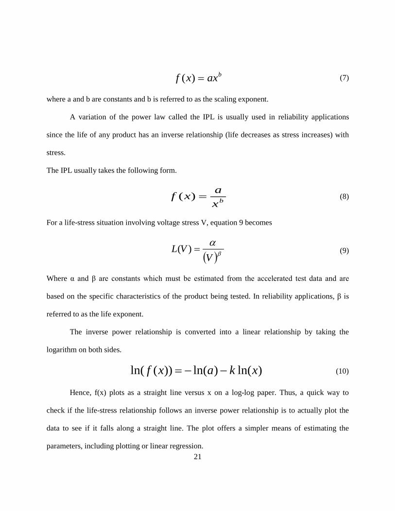
baxxf =)( (7)
where a and b are constants and b is referred to as the scaling exponent.
A variation of the power law called the IPL is usually used in reliability applications
since the life of any product has an inverse relationship (life decreases as stress increases) with
stress.
The IPL usually takes the following form.
bx
axf =)( (8)
For a life-stress situation involving voltage stress V, equation 9 becomes
( )β
αV
VL =)( (9)
Where α and β are constants which must be estimated from the accelerated test data and are
based on the specific characteristics of the product being tested. In reliability applications, β is
referred to as the life exponent.
The inverse power relationship is converted into a linear relationship by taking the
logarithm on both sides.
)ln()ln())(ln( xkaxf −−= (10)
Hence, f(x) plots as a straight line versus x on a log-log paper. Thus, a quick way to
check if the life-stress relationship follows an inverse power relationship is to actually plot the
data to see if it falls along a straight line. The plot offers a simpler means of estimating the
parameters, including plotting or linear regression.

22
The acceleration factor computations for the inverse power model are shown in the
equations below:
n
u
s
s
uus V
VVTVTnVVAFVAF
===
)()(),,()( (11)
Note: T in equation 12 refers to the time to failure.
When sV > uV , AF ( sV , uV , n) > 1. where uV and n are understood to be product use (or other
baseline) voltage and the material-specific exponent, respectively, and AF (V) = AF ( sV , uV ,n)
denotes the acceleration factor.
The inverse power law relationship is generally considered to be a good empirical model
for the relationship between life and the stress levels of certain accelerating variables, especially
those that are non-thermal in nature. Nelson [1] points out some of the applications including,
• Electrical insulations and dielectrics in voltage endurance tests,
• Incandescent lamps (IEC publ. 64), and
• Simple metal fatigue due to mechanical loading.
“Even though the inverse power relationship is an empirical relationship, a physical
motivation can be provided for certain failure modes. The physics is now investigated for
electrical insulations. The ideas extend, however to, other dielectric materials, products, and
devices like insulating fluids, transformers, and capacitors. In applications, insulation should not
conduct electric current. Insulation has a characteristic dielectric strength which can be expected
to be random from unit to unit. The dielectric strength of a specimen operating in a specific

23
environment at a specific voltage may degrade with time. When the specimen’s dielectric
strength falls below the applied voltage stress, there will be a flash-over, short circuit, or other
failure-causing damage to the insulation. This failure mechanism lends itself to the inverse-
power relationship” [2].
The material break-down strength also degrades over time due to the chemical
degradation. The time to failure of this mechanism can be accelerated by increasing the voltage
as this increase in voltage essentially increases the rate of the underlying electrochemical
degradation processes. Acceleration can also be achieved by decreasing the thickness of the
dielectric.
The inverse power relationship has been successfully used to model several other
non-thermal stress relationships. The following are some of the acceleration models of the
inverse-power functional form developed for diverse applications.
2.2.4.4 Coffin-Manson Relationship
“The inverse power relationship is used to model fatigue failure of metals subjected
to thermal cycling. The typical number N of cycles to failure as a function of the
temperature range ΔT of the thermal cycle is
BTAN
∆=
(12)

24
Here A and B are constants characteristic of the metal and test methods cycle. The
relationship has been used for mechanical and electronic components. For metals, B is near 2.
For plastic encapsulants and microelectronics B is near 5” [1].
2.2.4.5 Palmgren’s Equation
“Life tests of roller and ball bearings employ high mechanical load. In practice, life (in
millions of revolutions) as a function of load is represented with Palmgren’s equation for the 10th
percentile, B10, of the life distribution, namely,
p
PCB )(10 =
(13)
Where C is a constant called bearing capacity, p is the power, and P is the equivalent load in
pounds. For steel ball bearings p=3 is used, and for steel roller bearings p=10/3 is used”. [1].
2.2.4.6 Taylor’s Model
“Taylor’s model is used for the median life τ of cutting tools namely,
mVA
=τ
(14)

25
Here V is the cutting velocity (feet/sec), and both A and m are constants depending on factors
like tool material and geometry. For high strength steels, m = 8, for carbides m= 4, and for
ceramics m=2” [1].
2.2.5 Multi Stress Models
2.2.5.1 Generalized Eyring Relationship
The generalized Eyring relationship offers a general solution to the problem of additional
stresses. The generalized Eyring relationship has been typically used in accelerated stress tests
with temperature and another non-thermal stress. It also has the added advantage of having a
theoretical derivation based on quantum mechanics.
The Eyring model written for temperature and a non-thermal stress (typically voltage)
takes the form
TVDVC
TBA
eT
VTL⋅+⋅++
=1),(
(15)
T is the temperature stress and V is voltage stress. The parameters A and B are used to estimate
the temperature effect. C is used to model the voltage and D is the interaction term. Additional
factors can be added to the right of the non-thermal stress to extend this relationship. It must be
noted that the Eyring relationship is a special case of the generalized Eyring relationship which
does not have the voltage and the interaction term.

26
Typical two-stress models such the temperature-humidity model and the power-
exponential model do not account for the interaction terms, and assume that the two stresses are
independent. The generalized Eyring model solves this problem by incorporating an interaction
term. “However, in an independent two-stress model, separate acceleration factors can be
obtained for each stress by varying that stress while keeping the others constant; multiplying
these individual acceleration factors yields the acceleration factor for the life-stress model. In the
case of the generalized Eyring relationship, the two acceleration factors cannot be separated” [5].
“Another difficulty is finding the proper functional form, or units, with which to express
the non-thermal stresses. Temperature is in degrees Kelvin. But what should be the unit for
voltage for example? The theoretical model derivation does not specify, so the experimenter
must either work it out by trial and error or derive an applicable model using arguments from
physics and statistics” [6]. Nelson [1] presents two applications of the generalized Eyring model
of the above form:
• Capacitors: The first 1/T term was not used, and a transformed V (ln V) was used to
model voltage. The interaction term was assumed to be 0. The data was plotted on
Arrhenius paper (temperature on absolute scale, life and voltage in log scales). The
results are satisfactory for test data on low density polyethylene.
• Electromigration: A generalized Eyring model is used to model the failures due to
electromigration which depend on temperature (T) and current density (J). Black’s
formula for such situations is,

27
kTE
neAJJTL −=),( (16)
2.2.5.2 Generalized Log-Linear Model
When a test involves multiple accelerating stresses, a general multivariable relationship is
needed. The general log-linear relationship describes a life relationship as a function of a vector
of n variables (or covariates):
nnαβαβαβαβατ ++++= .....)ln( 3322110 (17)
Mathematically, the model can be expressed as an exponential model, expressing life as a
function of the stress vector α,
∑= =
+n
iii
e 10
)(βαα
βτ
(18)
This relationship can also be reduced to an exponential or power single stress relationship
by using a different transformation of β. For example, consider a single temperature stress
scenario of this model and a reciprocal transformation on β, such that β=1/T, then
TT eeeT1
010
1
)(α
ααατ +==
⋅+
(19)
If A= 0αe and α1=Ea/K, (21) reduces to an Arrhenius equation:
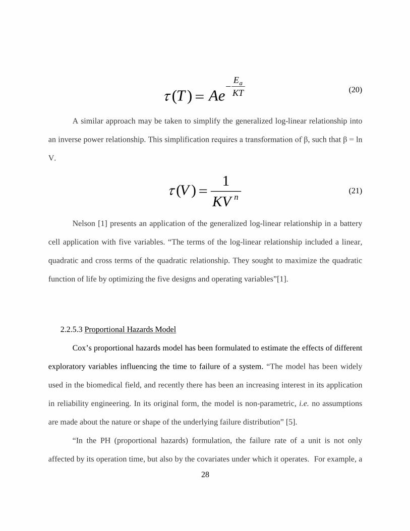
28
KTEa
AeT−
=)(τ (20)
A similar approach may be taken to simplify the generalized log-linear relationship into
an inverse power relationship. This simplification requires a transformation of β, such that β = ln
V.
nKVV 1)( =τ
(21)
Nelson [1] presents an application of the generalized log-linear relationship in a battery
cell application with five variables. “The terms of the log-linear relationship included a linear,
quadratic and cross terms of the quadratic relationship. They sought to maximize the quadratic
function of life by optimizing the five designs and operating variables”[1].
2.2.5.3 Proportional Hazards Model
Cox’s proportional hazards model has been formulated to estimate the effects of different
exploratory variables influencing the time to failure of a system. “The model has been widely
used in the biomedical field, and recently there has been an increasing interest in its application
in reliability engineering. In its original form, the model is non-parametric, i.e. no assumptions
are made about the nature or shape of the underlying failure distribution” [5]. “In the PH (proportional hazards) formulation, the failure rate of a unit is not only
affected by its operation time, but also by the covariates under which it operates. For example, a

29
unit may have been tested under a combination of different accelerated stresses such as humidity,
temperature, voltage, etc. It is clear that such factors affect the failure rate of the unit. The
proportional hazards model assumes that the failure rate (hazard rate) of a unit is the product of a
baseline failure rate, which is a function of time only, and a positive function independent of
time, which incorporates the effects of a number of covariates such as humidity, temperature,
pressure, voltage, etc” [5]. The failure rate of a unit is then given by
)..(0
2211)(),( nn xxxetxt βββλλ ++⋅= (22)
The base failure rate (λ0) and the coefficients β1, β2... βn are estimated from the data. The
corresponding reliability function is,
)..2211(
)]([),( 0nxnxxetRxtR
βββ ++
= (23)
Where,
∫=
−t
dtt
etR 00 ])([
0 )(λ
(24)
“An advantage of this model is that it allows for simultaneous analysis of continuous and
categorical variables. Categorical variables are variables that take discrete values such as the lot
designation products from different manufacturing lots. Additionally, zero can be utilized as a
stress when used as a categorical variable (i.e. on/off)” [5]. This property of the PH model lends
itself to analysis of field reliability data, where the covariates represent variables such as
operating environment, use-rate, interfacing equipment, etc.

30
The disadvantage of the non-parametric nature of the model is that the PH model cannot
be used to extrapolate to another percentile in the use-stress distribution (it can extrapolate in
stress but not in time). “Another disadvantage of the PH model is that its life distribution and the
life-stress relationship are complex. Moreover the spread and shape of the distribution of log life
generally depends on the variables in a complex way” [1]. Parametric models modeling the same
scenarios have simpler form. Computer programs such as ALTA® are usually required to
evaluate this model.
2.2.6 Survey of other Acceleration Models
The six acceleration models presented above are the most commonly used life-stress
relationships. This section briefly surveys a number of other relationships.
2.2.6.1 Elastic Plastic Relationship for Metal Fatigue
The following model has been used for metal fatigue over a wide range of stresses
ba BNANS −− += (25)
Where
• N is the number of cycles,
• S is the total strain due to elastic and plastic components, and
• A, a, b and B are parameters that must be estimated from the data.

31
“The elastic term AN-a usually has a value in the range of 0.1 to 0.2 and the plastic term BN-b
usually has a b value in the range 0.5 to 0.7. However, it must be noted that the fatigue life of
metals is complex and no one S-N curve is universally applicable. ASTM (American Standard
for Testing of Materials) 744 proposed some of the fatigue curves. Some applications involving
temperature and other variables employ polynomial fatigue curves. Such polynomial curves
merely smooth the data. They have no physical basis” [1].
2.2.6.2 Quadratic and Polynomial Relationships
The quadratic relationship for log of nominal life τ as a function of (possibly
transformed) stress x is
2210)log( xx γγγτ ++= (26)
This relationship is sometimes used when a linear relationship ( x10 γγ + ) does not adequately fit
the data. For example, the linear form of the IPL may be inadequate. “A quadratic relationship is
often adequate over the range of test data, but it can err if extrapolated much outside. It is best to
regard this model as a function fitted to data rather than a physical relationship based on theory”
[1].
“A polynomial relationship for the log of nominal life τ as a function of possible
transformed stress x is:
kk xxx γγγγτ ...)log( 2
210 +++= (27)

32
Such relationships are used for metal fatigue data over the range of the data. A polynomial for K
≥ 3 is virtually worthless for extrapolation, even short extrapolation” [1].
2.2.6.3 Temperature - Humidity Model
“Many accelerated life tests of epoxy packaging for electronics employ high temperature
and Reliative Humidity (RH). Peck surveys such testing and proposes an Eyring relationship for
life” [1].
kTE
n eRHA −= )(τ (28)
This relationship is also known as Peck’s relationship. The parameters n and E are to be
estimated from data. “Data he uses to support the relationship yields estimates n =2.7 and E =
0.79 eV. The terms A and k are constants. The equation can also be modified to use with
voltage instead of the RH term. Another variation of Peck’s equation is as follows.
kTE
RHB eeA .−⋅=τ (29)
Equation 29 differs little from the Peck’s relationship relative to uncertainties in data”
[1]. B is a constant. Another variation of this relationship uses a similar exponential relationship
for temperature (T) and humidity (U), α and β are parameters to be estimated from data.
UTUT AeeDeCβαβα
τ+
=⋅⋅= ]].[[ (30)

33
It must be noted that all three variations of this model assume independence (no interaction)
between the two stresses under study.
2.2.6.4 Zhurkov’s Relationship
Zhurkov’s relationship is used to model the failure mechanism with respect to the rupture of
solids at absolute temperature T and tensile stress S:
)](}[(
kTSD
kTB
Ae−
=τ (31)
“Equation 31 is a variation of a Eyring relationship with C = 0 and a minus sign for D.
Zhurkov motivates this relationship with chemical kinetic theory, and he presents data on many
materials to support it. He interprets B as the energy to rupture molecular bonds and D is a
measure of disorientation of the molecular structure” [1].
This model is used in fracture mechanics of polymers, as well as a model for the electro-
migration failures in aluminum thin films of integrated circuits. In the last case, the stress factor
x is current density. The model is widely used for reliability prediction problems of mechanical
and electrical (insulation, capacitors) long-term strength.
2.2.6.5 Exponential-Power Relationship
A combination of exponential and power relationships can also be used in a life-
stress relationship. An exponential-power relationship that describes the effect of single stress on
life is as follows:

34
)( 2
10γγγτ xe −=
(32)
“This model is used in MIL-HDBK-217E, where x is often voltage or inverse of absolute
temperature. The relationship has three parameters and thus it is not linear on any plotting paper”
[1]. 210 ,, γγγ are parameters to be estimated from the data.
Another model that uses a combination of exponential and power relationships is the
temperature-non-thermal model. The non-thermal stress used in the following equation is
voltage. The constants A and K are simplified into C in the final equation. B is another
constant that must be estimated from the data. The temperature-non-thermal model is:
TB
n
TB
nnTB
eV
CeVK
AKV
eAVT−
⋅=⋅⋅=⋅⋅=
1]1[][),(τ
(33)
This model also assumes independence between temperature and the non-thermal stress.
2.2.6.6 Non-Linear Relationships
Most acceleration models use a linear relationship. Engineering theory may suggest
relationships that are non-linear in nature. Nelson [1] gives an example of such a non-linear
relationship. This test considers the time to breakdown of an insulating fluid between parallel
disk electrodes. The voltage across the electrodes increases linearly with time at different rates R
(volts per second). Electrodes of various areas were employed. The assumed distribution for
time to breakdown is Weibull with parameters α and β shown in equation 34 [1].

35
1
1
1 ,),( 1
0γβγα
γ
γ =
⋅=
eARAR (34)
2.2.7 Degradation Models
Designs of high reliability products require that the respective product components have
an extremely high reliability. This high reliability presents a problem in collecting test data, as no
failures occur during those tests even at an accelerated stress level. In some components it, may
however, be possible to measure the degradation of a specific characteristic in time.
“Degradation analysis involves the measurement and extrapolation of degradation or
performance data that can be directly related to the presumed failure of the product in question” .
In some cases, it is possible to directly measure the degradation over time, as with the wear of
brake pads or with the propagation of crack sizes (non-catastrophic). In other cases, direct
measurement of degradation might not be possible without invasive or destructive measurement
techniques. In such cases, the degradation of the product can be estimated through the
measurement of certain performance characteristics. A level of degradation or performance at
which a failure is said to have occurred needs to be defined” [3].
Accelerated degradation tests are used to accelerate such degradation mechanisms by
applying higher stresses and predicting the time to failure. The resultant data is then used to
predict the life characteristics at use level. Accelerated degradation models show the relationship

36
between measured degradation and stress level. Nelson [1] states some of the “assumptions for
such models:
• Degradation is not reversible, such that the performance gets monotonically worse. Such
models do not apply to products that improve with exposure.
• Usually a model applies to a single degradation mechanism.
• Degradation of the specimen performance before the tests starts is negligible.
• Performance is measured with negligible random error”.
A simple degradation relationship for typical log performance µ (t) is a simple linear function
of product age t:
tt ')( βαµ −= (35)
Where
• µ(t) is considered as the mean or median of the distribution of log performance at time t,
• α is the intercept coefficient which corresponds to the log performance at time 0, and
• β’ is the degradation rate which is assumed to be constant over time, but is a function of
accelerated stress.
If the product fails when typical log performance degrades to a value fµ the time to failure
is given by
'βµα ft
−= (36)
37
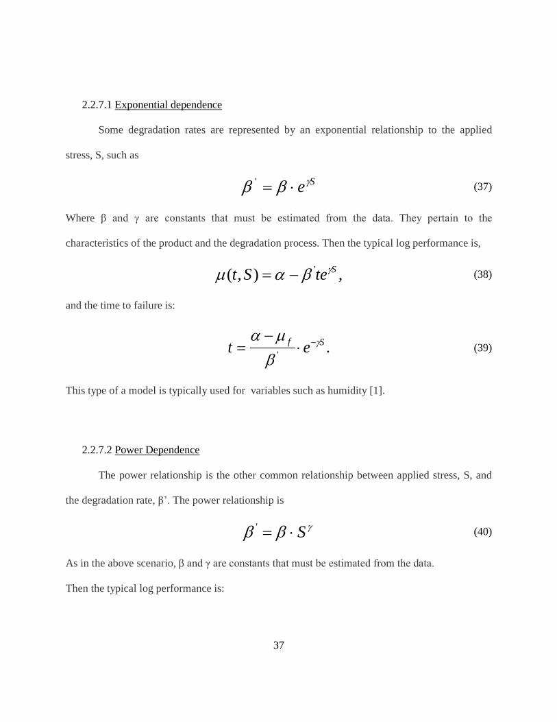
2.2.7.1 Exponential dependence
Some degradation rates are represented by an exponential relationship to the applied
stress, S, such as
Seγββ ⋅=' (37)
Where β and γ are constants that must be estimated from the data. They pertain to the
characteristics of the product and the degradation process. Then the typical log performance is,
,),( ' SteSt γβαµ −= (38)
and the time to failure is:
.'Sf et γ
βµα −⋅
−=
(39)
This type of a model is typically used for variables such as humidity [1].
2.2.7.2 Power Dependence
The power relationship is the other common relationship between applied stress, S, and
the degradation rate, β’. The power relationship is
γββ S⋅=' (40)
As in the above scenario, β and γ are constants that must be estimated from the data.
Then the typical log performance is:

38
,),( ' γβαµ tSSt −= (41)
and the time to failure is
.'
γ
βµα
St
f
−
= (42)
This model is often used for electronics and dielectrics where S is the voltage [1]. Similar models
can be constructed for Arrhenius and Eyring relationships.
2.2.8 Models for Time-Varying Stresses
All the models presented thus far use a constant accelerated stress. Sometimes it may be
necessary to vary (usually increase) the stress in order to generate failures quickly. This variation
is highly desirable given the high reliability of the products under test and increased pressure to
reduce “time to market” by reducing the product development time.
“The most basic type of time-varying stress test is a step-stress test. In step-stress
accelerated testing, the test units are subjected to successively higher stress levels in
predetermined stages, and thus a time varying stress profile. The units usually start at a lower
stress level, and at a predetermined time or failure number, the stress is increased and the test
continues. The test is terminated when all units have failed, or when a certain number of failures
are observed, or until a certain time has elapsed” [5]. Figure 4 below shows a typical step-stress
profile.

39
Figure 4: A step stress profile
Another commonly used time varying stress is the ramp tests or progressive stress tests.
In these tests, the stress monotonically increases at a specified rate until failure. The rate at which
the stress is varied may be changed to achieve different stress cells. Figure 5 shows a typical
ramp-stress profile. It is also possible to have a combination of a step stress and progressive
ramp type stress profiles in a single accelerated test.
Figure 5: Ramp or Progressive Stress test
“When dealing with data from accelerated tests with time-varying stresses, the life-stress
model must take into account the cumulative effect of the applied stresses. Such a model is

40
commonly referred to as a “cumulative damage” or “cumulative exposure” model” [5]. Nelson
[1] presents the following derivation for the power-Weibull model.
The cumulative distribution function (CDF) of the cumulative (step-stress) damage model
is given by:
βε−−= etF I 1)(0 (43)
Where β is the Weibull shape parameter.
Here the cumulative exposure ε for the failure mode is
I
I
ααααε ∆
++∆
+∆
+∆
= ...3
3
2
2
1
1 (44)
Where
pi
i VK
=α (45)
and
.1−−=∆ iii tt (46)
The cumulative exposure now becomes,
P
I
iPP
VV
tt
VV
tt
VV
tt
−+
−+
−= −
0
1
2
0
12
1
0
1 .....0)(ε (47)
For a stress V and a scale parameter, )(Vθ , the general form of the CDF can be given by

41
.)(
);(
=
VtGVtF
θ (48)
“Here G is the assumed cumulative distribution with the scale parameter set to 1. For a ramp
stress model, where the stress, )(tV , is a function of time, the distribution scale parameter,
),( xVα , is a function of time ),()( xtt αα = , where x is a constant stress variable” [1]. The
cumulative exposure )(tε now becomes:
[ ]∫=t
xtVdtt
0 ),()(
αε (49)
Where )(tε is a function of xtV ),( and the model parameters. The CDF for this scenario becomes
[ ] [ ])(,)"(";0 tGxtVtF ε= (50)
Here G is the assumed cumulative distribution with the scale parameter set to 1. )"(" tV in quotes
emphasizes that )(tV does not merely replace the V in the constant stress model [1].
“One of the applications of cumulative damage model is the Miner’s rule. It is a
deterministic model based on linear damage theory. Its inadequacies in metal fatigue are well
known but it is frequently used. The cumulative damage model discussed above is a probabilistic
extension of the Miner’s rule” [1].
Ramp or progressive stress types are frequently used on electronics and dielectrics to
reveal failure modes such as dielectric breakdown. Such tests are gaining increasing popularity in
situations where extremely specialized test equipment is required or when a small number of

42
systems are available to test. The primary motivation for the time-varying stress is, of course, the
time saved in the test by inducing failure quicker.
Despite the advantages that the time varying stress tests offer over the constant stress
tests, they have the following limitations as stated by Nelson [1]:
• Step-stress and progressive stress tests are used to induce failure quickly. “However the
accuracy of the estimates from such a test is inversely proportional to its length. Such
tests yield no greater accuracy than the constant stress test of the same length. However
the asymptotic theory is a better approximation when there are many failures” [1].
• Typically, “it is easier to hold a stress constant than to vary it exactly in a prescribed
manner. Thus varying-stress tests have an added source of experimental error” [1].
• “Failure mechanisms should remain relatively constant over a stress range. That is, the
relationship between log stress and log life is linear over the range of stresses involved”
[1].
• The physical phenomenon under study must have a cumulative damage property. Such
tests may not be used on memory-less failure mechanisms such as yielding or melting.
The cumulative damage models work effectively for failure mechanisms such as fatigue
and dielectric breakdown.

43
2.2.9 Survey of Recent Research – Acceleration Models
Several of the recent research articles ([36], [38], [17], [16]) in ALT use models of the
inverse power relationship category. Much of the work done in fatigue ([13], [14], [18]) and
fracture mechanics also develops relationships that constitute a power function.
Some authors have demonstrated a better fit of a new model to certain applications where
other models have been historically considered adequate. Rodriguez [49] demonstrated that the
PH model is a better fit in situations where two temperature related stresses are used. Historically
Arrhenius type models have been used in such applications. Another PH model based on mean
residual life has been proposed by Zhao [53].
Other authors have proposed degradation type models ([54], [41]) and cumulative
damage models [60] as alternatives to commonly used constant stress failure models. Models
based on the transfer functions such as the PH model have also been used in certain applications.
Such non-parametric or semi-parametric properties have been considered desirable in some
situations. The changing scale and shape (CHSS) model proposed by Bagnodivicus and Nikuln
[20] is one such alternative to the typically used parametric models and has both non-parametric
and semi-parametric estimation methods.
Some authors have also used hazard regression methods as alternatives to traditional
accelerated life test methods. One research study [33] proposes the extended hazards regression
(EHR) model for the effects of simulated temperature and voltage data. Such models however,
have not been widely used on most engineering scenarios of ALT.

44
Models that establish relationships for more than one stress have also been an area of
increased research. The generalized log-linear model [9] and the generalized multiplicative
model [27] are examples of such applications. Several authors ([12], [13],
[16],[17],[19],[40],[44],[45]) have used a combination of two single stress models to achieve the
same goal. These examples demonstrate the fact that a multi-variable scenario is unavoidable in
many engineering situations as most of the common failure modes have multivariable
relationships.
Empirical models have also been developed in many situations. A semi-parametric
empirical model was developed as an alternative to the commonly used Basquin model for use
on metal fatigue [12]. A modified and extended version of the Paris equation has been created by
Guerin et al [14] to model the effects of temperature and mechanical loading on fatigue cracking.
It must be noted that much of the current research and applications have been focused on
mechanical failure modes such as metal fatigue and thermal fatigue used in electronic
applications. Swain [10] proposes an accelerated life testing methodology to model the bio-
fouling mechanism common to sub-sea structures. He uses agitation and aeration as accelerating
variables. Even though exponential [61] and power [64] relationships have been used as models
for pressure variables, no demonstrated research has been noted to show the suitability of such
models for sub-sea applications.

45
2.3 Parameter Estimation
Parameter estimation is the process of estimating the life characteristics of the product at
the use level based on the data collected at the stress level(s). The acceleration model (life-stress
relationship and life distribution) and the test data provide the basis for parameter estimation.
The four methods commonly used for parameter estimation are:
1. Reliability data plotting,
2. Least-squares method,
3. Maximum likelihood method, and
4. Bayesian estimation.
2.3.1 Reliability Data Plotting Method
The reliability data plotting is the simplest and least accurate of the four methods used for
parameter estimation and involves estimation of the parameters using reliability data plots. For
example, consider a scenario of life data that follows a Weibull distribution and any life stress
relationship that can be linearized. The data is first plotted on Weibull paper to estimate the
shape and scale parameter at the different stress levels. The shape parameter can be expected to
be the same at different levels, whereas the scale parameters computed at the different stress
levels are used to estimate the scale parameter at the use level. This computation can be achieved
analytically by using the life stress relationships or by simple plotting methods. An example of a
Weibull plot, where the parameters are estimated, is given in the Figure 6.
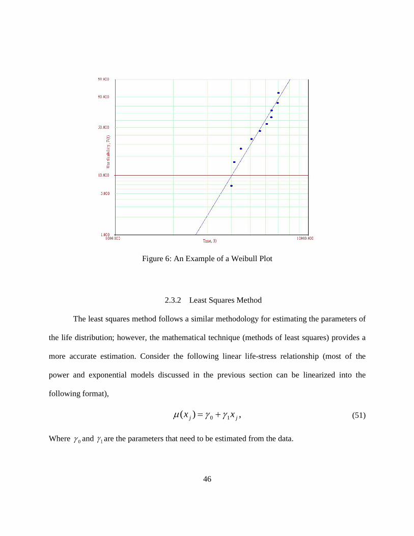
46
Figure 6: An Example of a Weibull Plot
2.3.2 Least Squares Method
The least squares method follows a similar methodology for estimating the parameters of
the life distribution; however, the mathematical technique (methods of least squares) provides a
more accurate estimation. Consider the following linear life-stress relationship (most of the
power and exponential models discussed in the previous section can be linearized into the
following format),
,)( 10 jj xx γγµ += (51)
Where 0γ and 1γ are the parameters that need to be estimated from the data.

47
Consider a random sample of n units that are all run to failure. There are J stress levels
and jn units tested at each stress level .,....3,2,1, Jjx j = ijy denotes the time to failure of test
unit I at test stress jx . The sample average jy and sample standard deviation js are calculated
for each test stress. Calculate the grand average of all data as follows
nxnxnx jj /)...( 11 += (52)
nynyny jj /)...( 11 += (53)
The sums of squares are calculated as follows,
2
1
2
1
2
11)( ynyyyS
jj n
iij
J
j
n
iij
J
jyy −=−= ∑∑∑∑
==== (54)
22211
2211 ....)(....)( xnxnxnxxnxxnS jjjjxx −+=−+−= (55)
yxnyxnyxnyxxnyxxnS jjjjjjxy −+=−+−= ...)(...)( 111111 (56)
The least squares estimates of 1γ and 0γ are
xxxy SSc /1 = (57)
xcyc 10 −= (58)
These two parameters will help us estimate the life characteristics at any given stress level based
on the life stress relationship.
“The least squares analysis of data involves assumptions about the model and data. Thus the
accuracy of estimates depends on how well the following assumptions hold” [1].

48
• The (transformed) relationship between the stress and life is linear,
• The shape parameter of the life distribution remains constant at all stress levels, and
• The type of distribution does not change among the stress levels.
“Some estimates are accurate enough even when assumptions are far from satisfied others
may be quite sensitive to an inaccurate model or faulty data. A simple test for linearity can be
performed by verifying if the sample means of log life are statistically significantly far from the
fitted straight line” [1]. Nelson [1] points to certain key reasons why test results may falsely
show a non-linear relationship, namely:
1. “Inaccurate stress levels (wrong measurement or not held constant)
2. Malfunctioning test equipment. (for example failure of a given specimen in a rack,
caused all other units to fail , due to lack of electrical isolation)
3. Differing test specimens due to differing raw materials, manufacturing handling and
personnel. (for example specimens made by third shift failed sooner)
4. Differing test conditions due to uncontrolled variables other than stress. (for example
temperature increases with voltage used as the accelerating stress)
5. Blunders in recording analyzing and transcribing the data” [1].
“Analytical methods such as least squares have both advantages and disadvantages when
compared to the graphical techniques. Analytical methods are objective; that is, if two people use

49
the same analytic methods on a set of data they get exactly the same result. This consistency is
not true of graphical methods, but two people will reach the same conclusions from graphical
methods. Such a method also indicates the accuracy of the estimates by confidence interval and
standard error. Statistical uncertainties in estimates of product life are usually large and startling.
The accuracy is important if the graphical methods indicate that the information is accurate
enough for practical purposes” [1].
A disadvantage of analytic methods such as the least squares method is that the
computations are too laborious and may require a computer program such as Minitab®. However,
graphical methods are user-friendly, and there are software programs that do the graphical
analysis.
2.3.3 Maximum Likelihood Method
Maximum likelihood (ML) is perhaps the most versatile method for estimating the
parameters from the accelerated test data. The appeal of ML stems from the fact that it can be
applied to a wide variety of statistical models and kinds of data, where other popular methods
such as least squares, are not, in general, satisfactory.
The ML method usually starts with a set of data, and an acceleration model which has
been selected based on a physics of failure study. The likelihood function can be viewed as the
probability of observed data written as a function of the acceleration model’s parameters. The
acceleration model fitted to data consists of a combined distribution whose parameters express
the relationship between stress and life and also the characteristics of the life distribution at any

50
given stress level. Let us consider these parameters as 1θ through nθ . The probability density of
a failure at time t is
,/)..;()..;( 11 dttdFtf nn θθθθ = (59)
Each distribution parameter can be expressed as a function of J test observations Jtt ....1
(complete or censored) and the estimates of the model parameters nγγ ...1 .
)......;...( 1111 nJtt γγθθ = (60)
)...;...( 11 nJnn tt γγθθ = (61)
The ML method estimates the parameters of the distribution based on the (log) likelihood
of a set of data. The data is usually an exact value (failure time) or it can be right censored, left
censored and interval type data is also possible, but is very uncommon in a modern engineering
scenario with equipment to record the observed time. The likelihood for each type of data is as
follows.
2.3.3.1 Exact Failures
Suppose a unit has a failure time it , then its likelihood can be expressed by the
probability density function of the combined distribution at time it .
iL is the “probability” of an observed failure at time it :
)....;( 1 niiii tfL γγ= (62)

51
2.3.3.2 Right Censored
Suppose the given test unit was censored without failure at time .it Then its likelihood
can be expressed as the reliability function of the combined distribution at time it .
Then iL is the “probability” of the unit’s time to failure being beyond it :
).....;(1 1 niiii tFL γγ−= (63)
It is assumed that test observations are independent. Then the likelihood, L , of having a
data set with J test observations is the combined probability of the J test outcomes.
JLLLL ...21 ××= (64)
Equation 68 can be simplified by a log-likelihood function which is,
)ln(...)ln()ln( 21 JLLL ++=Λ (65)
This log-likelihood function is hence a function of the parameter estimates nγγ ...1 .
)...( 1 nγγΛ=Λ (66)
The maximum likelihood estimates nγγ ˆ...ˆ1 of nγγ ...1 are the values that maximize the log
likelihood over the allowed ranges of nγγ ...1 , thus these estimates are the values that maximize
the probability (likelihood) of the test data. The estimates are usually obtained using calculus.
Namely, set equal to zero the n derivates of the log-likelihood function with respect to nγγ ...1
and solve the equations for estimates nγγ ˆ...ˆ1 :

52
0/)...( 11 =∂Λ∂ γγγ n (67)
…..
0/)...( 1 =∂Λ∂ nn γγγ (68)
Usually these non-linear equations are solved using numerical methods or by using software
such as ALTA®.
Nelson [1] suggests that “for some models and data the estimates may not exist; for
example, they may have physically unacceptable values such as infinity or zero (say for standard
deviation). For most models and data the ML estimates are unique”[1].
After obtaining nγγ ˆ,...,ˆ1 , their covariance matrix is calculated from the Fisher matrix to
obtain the confidence interval for various parameter estimates. The Fisher matrix is a NN ×
matrix of negative partial derivatives.
∂Λ∂−∂Λ∂−∂Λ∂−
∂Λ∂−∂Λ∂−∂Λ∂−∂Λ∂−∂Λ∂−∂Λ∂−
=
222
21
2
222
22
122
12
2122
12
/ˆ..../ˆ/ˆ
...........
/ˆ..../ˆ/ˆ/ˆ.../ˆ/ˆ
nnn
n
n
F
γγγγγ
γγγγγγγγγγ
(69)
The caret (ˆ) indicates that the derivative is evaluated at nγγ ˆ,...,ˆ1 .The inverse of F is the
local estimate of the covariance matrix for nγγ ˆ,...,ˆ1 . That is,

53
== −
)ˆvar(....)cov()cov(
...........
)cov(....)ˆvar()cov()cov(...)cov()ˆvar(
21
2212
1211
1
nnn
n
n
FV
γγγγγ
γγγγγγγγγγ
(70)
The variance in the above matrix is used to compute the normal confidence intervals of
the model parameters nγγ ...1 .
Let us consider an example of accelerated test data with F failures and S censored units
following an IPL-Weibull (inverse power law with Weibull distribution) model; this combined
distribution has the following form:
βββ )(1)(),( tKVnn n
etKVKVVtf −−= (71)
The maximum likelihood function will be used to estimate the required parameters β, K
and n. The likelihood function of the IPL-Weibull model can thus be derived as:
( ) .)()(ln1
'1
1∑∑
=
−−
=
−
=Λ
S
i
ni
nii
TKVi
ni
ni
F
ii TKVNeTKVKVN i
ni ββ
β
β
(72)
The parameters of the IPL-Weibull model can be estimated by differentiating (76) with
respect to each of these parameter estimates and equating to 0, thus solving for β, K and n using
numerical methods.
0,0,0 =
∂Λ∂
=∂
Λ∂=
∂Λ∂
nand
Kβ (73)
For example,

54
)ln()(
)ln()()ln(1
'
1
'
111
inii
S
i
nii
in
iin
i
F
iii
ni
F
ii
F
ii
TKVTKVN
TKVTKVNTKVNN
β
β
ββ
∑
∑∑∑
=
===
−
−+=∂Λ∂
(74)
ββ βββ )()( '
1
''
11i
ni
S
iii
ni
F
ii
F
ii TKVN
KTKVN
KN
KK ∑∑∑===
−−=∂
Λ∂ (75)
ββ βββ ))(ln())(ln()ln(
1
'
11i
ni
S
iiii
nii
F
iii
F
ii TKVVNTKVVNVN
n ∑∑∑===
−−=∂Λ∂
(76)
The Fisher matrix for the above scenario is :
1
2
222
2
2
22
22
2
2
)ˆ()ˆ,ˆ()ˆ,ˆ()ˆ,ˆ()ˆ()ˆ,ˆ()ˆ,ˆ()ˆ,ˆ()ˆ(
−
∂Λ∂
−∂∂Λ∂
−∂∂Λ∂
−
∂∂Λ∂
−∂
Λ∂−
∂∂Λ∂
−
∂∂Λ∂
−∂∂Λ∂
−∂
Λ∂−
=
nKnn
nKKK
nK
nVarKnCovnCovnKCovKVarKCovnCovKCovVar
β
β
βββ
ββ
βββ
(77)
The confidence bounds for the parameters β, K and n will be computed using the
information above.
Meeker [4] suggests that, maximum likelihood estimators are “optimal” in large samples.
More specifically, this means that ML estimators are consistent and asymptotically (as the
sample size increases) efficient. That is, among the set of consistent competitors, none has a
smaller asymptotic variance. Besides Bayesian methods (which will be covered in the next
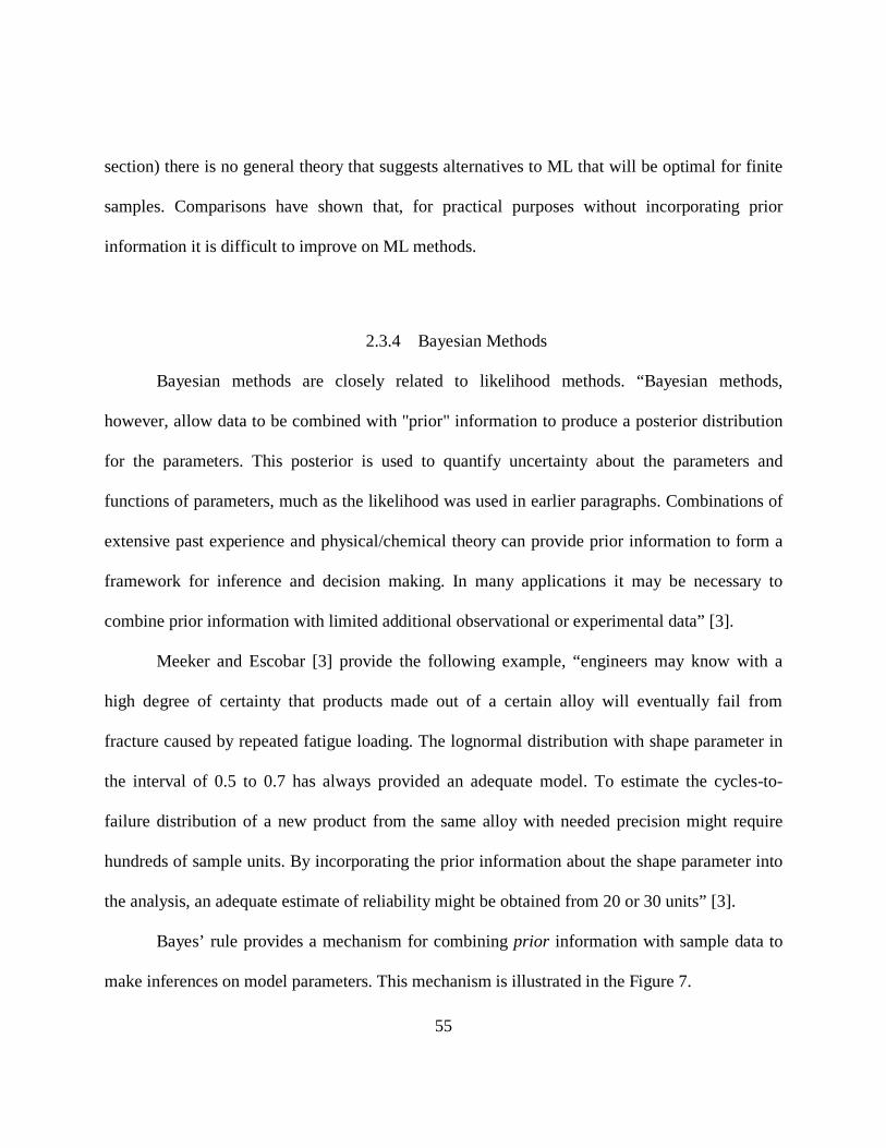
55
section) there is no general theory that suggests alternatives to ML that will be optimal for finite
samples. Comparisons have shown that, for practical purposes without incorporating prior
information it is difficult to improve on ML methods.
2.3.4 Bayesian Methods
Bayesian methods are closely related to likelihood methods. “Bayesian methods,
however, allow data to be combined with "prior" information to produce a posterior distribution
for the parameters. This posterior is used to quantify uncertainty about the parameters and
functions of parameters, much as the likelihood was used in earlier paragraphs. Combinations of
extensive past experience and physical/chemical theory can provide prior information to form a
framework for inference and decision making. In many applications it may be necessary to
combine prior information with limited additional observational or experimental data” [3].
Meeker and Escobar [3] provide the following example, “engineers may know with a
high degree of certainty that products made out of a certain alloy will eventually fail from
fracture caused by repeated fatigue loading. The lognormal distribution with shape parameter in
the interval of 0.5 to 0.7 has always provided an adequate model. To estimate the cycles-to-
failure distribution of a new product from the same alloy with needed precision might require
hundreds of sample units. By incorporating the prior information about the shape parameter into
the analysis, an adequate estimate of reliability might be obtained from 20 or 30 units” [3].
Bayes’ rule provides a mechanism for combining prior information with sample data to
make inferences on model parameters. This mechanism is illustrated in the Figure 7.
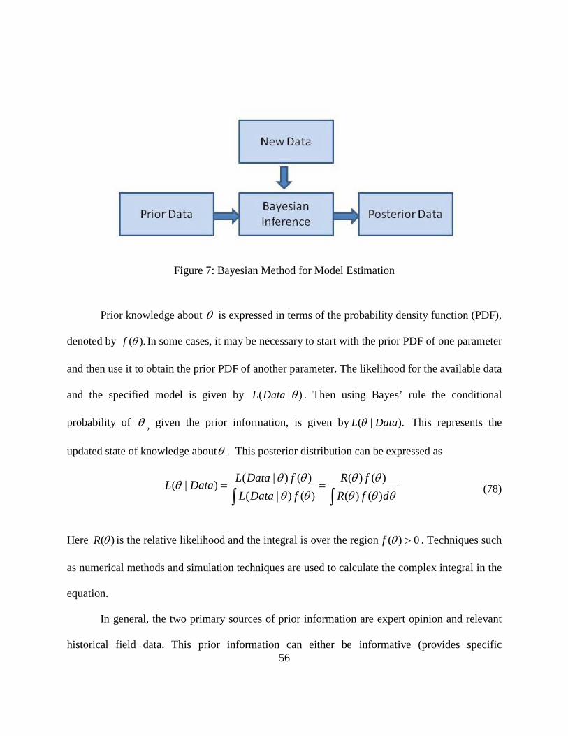
56
Figure 7: Bayesian Method for Model Estimation
Prior knowledge about θ is expressed in terms of the probability density function (PDF),
denoted by ).(θf In some cases, it may be necessary to start with the prior PDF of one parameter
and then use it to obtain the prior PDF of another parameter. The likelihood for the available data
and the specified model is given by )|( θDataL . Then using Bayes’ rule the conditional
probability of θ , given the prior information, is given by ).|( DataL θ This represents the
updated state of knowledge aboutθ . This posterior distribution can be expressed as
∫∫==
θθθθθ
θθθθθ
dfRfR
fDataLfDataLDataL
)()()()(
)()|()()|()|( (78)
Here )(θR is the relative likelihood and the integral is over the region 0)( >θf . Techniques such
as numerical methods and simulation techniques are used to calculate the complex integral in the
equation.
In general, the two primary sources of prior information are expert opinion and relevant
historical field data. This prior information can either be informative (provides specific

57
information about model parameters) or non-informative (does not provide specific information
about model parameters).
2.3.4.1 Prior Information from Expert Opinion
The elicitation of a prior distribution for a single parameter may be straightforward if
there has been considerable experience in estimating or observing estimates of that parameter in
similar situations. For a vector of parameters, however, the elicitation and specification of a
meaningful combined distribution is very difficult since it is difficult to elicit opinion on
dependences among model parameters [3]. Also it may not be reasonable to elicit expert opinion
about parameters from an acceleration model, when those parameters have no physical meaning
(the life exponent used in the inverse power law is a good example.)
A general approach is to elicit information about particular quantities or parameters that,
from past experience, can be specified approximately independently. When there is informative
prior information, one elicits a general shape, form, or range of the distribution. When
information is non-informative, it is usually translated into a vague prior distribution such as a
uniform distribution with sufficiently wide interval [3].
2.3.4.2 Prior Information from Historical Field Data
Most engineering organizations have comprehensive field data, clearly documenting the
life data along with the corresponding failure mechanisms and corrective actions. Such data can
be used to compose informative or non-informative prior distributions. For example, while

58
conducting an ALT on a new product, one may use field data on similar fielded products to
construct informative prior distributions. Life data on similar lower level components and
subsystems may also be used. It is, however, important to carefully review the data for special
situations that may reduce the quality of the data, such as customer misuse or unexpected field
conditions beyond the specified field environment. Such data may essentially “contaminate” the
prior distributions resulting in inaccurate estimations of the posterior.
Combining non-informative prior distributions from field data to test data gives a
posterior pdf that is proportional to the likelihood. The posterior PDF can then serve as a prior
PDF for further updating with new data [3]. Meeker and Escobar [3] provide the following
examples of proper prior distributions:
• Normal prior distribution with mean and the standard deviation b so that
−
=b
ab
f norθφθ 1)(
, (79)
• Uniform prior distribution between a and b so that
,1)(
abf
−=θ (80)
• Beta prior distribution between specified a and b with specified shape parameters (allows for a more general shape), and
• Isosceles triangle prior distribution with base (range) between a and b.
For IPL-lognormal scenario with model parameters K, n and σ , the posterior combined
distribution is computed as follows,
),,()( σθ nKff = (81)
59
∫ ∫ ∫ ⋅⋅
=
K n
dKdndnKfnKDataLnKfDatanKLDatanKL
σ
σσσσσσ),,(),,|(
),,(|),,(|),,(0
0 (82)
Figure 8 shows the Bayesian updating of such distribution parameters:
Figure 8: Bayesian Estimation of model parameter.
“One of the most important differences between Bayesian methods and the likelihood
method of making inferences is the manner in which the nuisance parameters are handled.
Bayesian interval inference methods are based on a marginal distribution in which nuisance
parameters have been integrated out and parameter uncertainty can be interpreted in terms of
probabilities from the marginal posterior distribution” [3]. Bayesian and likelihood estimation
methods may give very similar results for relatively large samples or when prior information is
approximately uninformative, but for most scenarios Bayesian methods provide a clear
advantage over the ML methods in terms of accuracy (confidence bounds) and efficiency
(number of test units and test time).
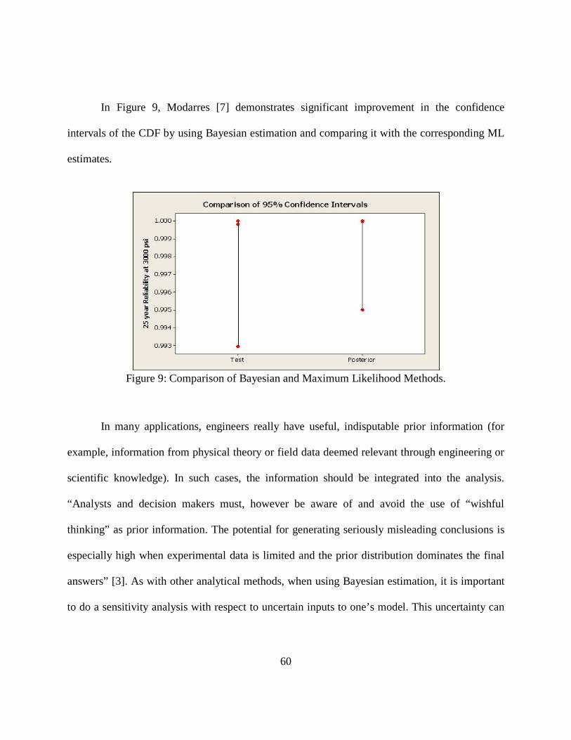
60
In Figure 9, Modarres [7] demonstrates significant improvement in the confidence
intervals of the CDF by using Bayesian estimation and comparing it with the corresponding ML
estimates.
Figure 9: Comparison of Bayesian and Maximum Likelihood Methods.
In many applications, engineers really have useful, indisputable prior information (for
example, information from physical theory or field data deemed relevant through engineering or
scientific knowledge). In such cases, the information should be integrated into the analysis.
“Analysts and decision makers must, however be aware of and avoid the use of “wishful
thinking” as prior information. The potential for generating seriously misleading conclusions is
especially high when experimental data is limited and the prior distribution dominates the final
answers” [3]. As with other analytical methods, when using Bayesian estimation, it is important
to do a sensitivity analysis with respect to uncertain inputs to one’s model. This uncertainty can

61
be explored by changing the values of the prior distributions and checking the effect that the
changes have on the final answer.
2.3.5 Survey of Recent Research – Parameter Estimation
Most of the research articles ([25], [31], [33], [35], [38], [50,], [53], [57], [59], [60])
reviewed in this survey use the ML method for estimating the parameters. ML is also the method
used in the commercially available software packages such as ALTA®.
Some authors, however, have pointed out the advantages of using Bayesian techniques.
Rodriguez [49] uses the Bayesian method to estimate the parameters of the PH model and
compares its estimates with the ML method. Batres [52] proposes a Bayesian estimation
approach to improve the reliability prediction using field performance data. He uses a simulation
based approach using the Markov chain Monte Carlo (MCMC) method to estimate the posterior
distributions. A program named WINBUGS® was used for this purpose.
Zhang [55] provides a detailed account on Bayesian life test planning by using a case of a
prior distribution with a Weibull shape parameter. He also presents two different approaches for
the estimation of a posterior distribution using numerical approximation and simulation methods
and compares the numerical results. The methods and recommendation for developing an
optimum Bayesian design are also presented.
Another research study [30] proposes Bayesian estimation methods for several time-
varying stress situations. A case study with censored and interval type data is discussed. Bunea
and Mazzuchi [24] present a Bayesian estimation method for a competing failure mode scenario.

62
Large and small data sets from motor insulation and industrial heaters were used for the study.
Pascual and Montepiedra [32] propose a Bayesian approach to estimate parameters from two
candidate models. The sensitivity of the results when either of those models does not fit the data
is investigated.
Several research articles ([28], [37], [48], [54], [56]) propose non-parametric and semi-
parametric estimation methods for models using transfer functions. However, the applicability
and use of such models and estimation methods have been found to be limited.
In general, ML methods for parameter estimation seem to dominate the accelerated test
methods used in the recent research. However, a recent trend seems to indicate increasing
interest in the use of Bayesian estimation method complementing the ML estimates with prior
information. The main reason behind this choice is to reduce test times and improve accuracy by
incorporating prior information. The reliability test programs in the sub-sea industry usually
involve such scenarios with expensive pressure vessels and other test fixtures. The diligent
tracking and availability of the field performance data including public databases such as
OREDA (offshore reliability data) can be potential sources of informative and non-informative
distributions. The Bayesian estimation method hence lends itself to the application of ALT in the
sub-sea industry. Therefore, the use of Bayesian methods to improve the quality of the ML
estimates will be considered in this research.
2.4 Accelerated Test Planning
Acceleration models and parameter estimation methods have been discussed thus far.
Proper planning is a prerequisite and is critical to the success of an ALT. For a well planned test,

63
the conclusions are clear with the simple analysis techniques, however, even the most
sophisticated parameter estimation methods and models cannot salvage a poorly planned test.
Some of the key factors to be considered in the planning of the tests are:
The experimental region: Testing over a wide range of the accelerating variable is
important to get the necessary precision. But testing beyond ranges where the failure mode
changes and the relevant acceleration model is inadequate must be avoided. On the other hand,
testing at the lower range which results in few or no failures during the time is also equally
undesirable. Such factors must be considered in establishing the experimental region.
Levels of accelerating variable: Appropriate levels must be chosen in the selected
experimental region; a minimum of two levels is needed to make any prediction. Three to four
levels are usually preferred. (There must be at least three test levels to check linearity or to fit a
non-linear relationship.) It is also helpful to get at least a few failures at a level closer to the use
stress to reduce uncertainties in extrapolation. A decision of using a constant or variable stress
profile must also be made.
Allocation of test units: It is important to get enough failures at each of the test levels.
More units must be allocated to the lower test level than to the higher test level. This allocation
compensates for the small proportion failing at low levels of the accelerating variable. This
allocation is also intuitively appealing as doing more tests at stress levels near the use level
reduces the uncertainties in extrapolation.
Testing at use conditions: Some experimenters, when conducting an ALT, choose to test
a small number of units at use conditions. These “insurance” units are typically tested to watch
64
for evidence of other potential failure modes, especially when it is possible to take degradation
measurements (or other parametric measurements) over time. Such units would not be expected
to fail and therefore will have no noticeable effect on estimates. For this reason, decisions about
allocation of the other units in the test can be made independently of decisions on the insurance
units [3].
Multi-variable tests: If possible the two accelerating variables may be combined into one
stress agent (for example, voltage x thickness can be treated as one stress agent instead of two
stress variables.) In other situations, proper experimental design must be developed to understand
the interaction and appropriate models must be chosen.
Team composition: “Accelerated test programs should be planned and conducted by teams
including individuals knowledgeable about the product and its use environment, the
physical/chemical/mechanical aspects of the failure mode, statistical aspects of the design and
analysis of reliability experiments” [3]
Failure mechanism: As a general rule accelerated stress tests must be conducted to obtain
information about the effect of a dominant stress variable on a specific failure mechanism. If
there is more than one failure mechanism, it is probable that the different mechanisms follow
dissimilar life-relationships at different rates. (Unless this difference is considered in the
acceleration model, the parameter estimation could result in incorrect conclusions.) Using failure
mode analysis and physical theory to understand the physics of failure will provide a better
physical basis for ALT. Conducting initial studies and experiments to understand the effect of
accelerating variables on life could also be helpful in planning the accelerated tests.

65
Accelerating variables: Appropriate stress variables that can accelerate the specific
failure mechanisms must be selected. “It is useful to investigate previous attempts to accelerate
failure mechanisms similar to the ones of interest. There are many research reports and papers
that have been published in the physics of failure literature” [3]. “Life of some products may be
accelerated through size, geometry and finish of specimens” [1].
Test units: Serious incorrect conclusions can result from an ALT, if test units will differ
from actual units. For example, factory manufacturing conditions will differ importantly from
those in a laboratory. Whenever possible, test units for an accelerated test should be
manufactured under actual production conditions using raw materials and parts that are the same
or as close as possible to those that will be used in actual manufacturing of units [3].
Test time: “Running an accelerated test until all units fail is generally inefficient; that is,
it wastes time and money. It is generally better to stop a test before all specimens fail. Then one
analyzes the censored data with the ML method which considers both failed and censored units.
Besides efficiency there is another reason to stop a test before all specimens fail, namely
accuracy of results. For example, for higher reliability products, one is usually interested in the
lower tail and little information is gained from the upper tail. Also suppose that the assumed life
distribution does not fit the data over the entire range of the distribution; that is, the model is
inaccurate. Then it is usually better to fit the distribution to the early failures of each test stress,
than to the later failures. This fit may be achieved by treating failures in the upper tail as if they
were censored at some earlier time. However, sometimes an important failure mode is active at
the design stress level and does not occur in the lower tail at the test stress levels. Rather it

66
occurs in the upper tail, then data from the upper tail is useful and terminating the test early
would miss that failure mode” [1].
2.5 The Research Gap Matrix
This literature review has discussed the different acceleration models used in the
reliability engineering community. The different parameter estimation methods and guidelines
for accelerated test planning are also discussed. The result of this literature survey suggests that
there is a significant research gap in the area of acceleration models, specifically addressing
hydrostatic pressure. This is clearly established in the research gap matrix in Figure 10.
The three major components of an accelerated test namely, physics of failure,
acceleration models, and parameter estimation form the major columns of this matrix. The
research in the physics of failure is usually carried out by the engineering community and hence
has been categorized into mechanical engineering related failure modes (MECH) and failures in
the electrical and electronics industry (EE). Similarly, the research in parameter estimation is
usually conducted by the statistical community and is classified into parametric, non-parametric,
and Bayesian estimation methods. Acceleration models, however, fall into a category where the
research requires both engineering and statistical skills, and hence is categorized both based on
the industry and also based on the parametric and non-parametric models. The acceleration
models and physics of failure studies are also categorized based on the various acceleration
variables such as temperature, humidity, hydrostatic pressure, mechanical stress, electrical stress,
and product related features.

67
It is to be noted that the engineering community focuses on the physical aspects of the
failure and accelerating variables it fails to experiment on the mathematical models and the
tendency is to use existing models. The statistical community, however, seems to focuses on the
mathematical aspects of the acceleration models but fails to develop relationships for a specific
failure mechanism or accelerating variables; such research often uses simulated data or data used
by other authors. This “silo” effect has been seen to act as an impediment in developing
acceleration models for specific applications which require good understanding of statistical
techniques and also an understanding of the engineering aspects of failure mechanisms. It is also
important to point out that research in areas such as Bayesian estimation which helps incorporate
prior engineering knowledge into statistical models has been increasingly adapted for research.
Reliability engineering provides a perfect platform for such research as this discipline
incorporates both of the necessary skills needed to execute this research.
The research gap matrix thus clearly shows a lack of research in acceleration models that
use hydrostatic pressure as an acceleration variable. It is also noted that most of the research in
EE community focuses on temperature, which is a critical failure mechanism in their area, while
the MECH community primarily focuses on mechanical stress. There is no research, however,
that focuses on critical variables such as pressure which is usually critical in the sub-sea
community.

68
Figure 10: The Research Gap Matrix
69
2.6 Discussions with Industry Experts
E-mail conversations with Dr. Wayne Nelson (09/24/07, 09/25/07, 11/01/07): Dr. Nelson
is one of the renowned consultants in the area of accelerated testing. Nelson’s book [1] is
considered by many practitioners and engineers to give the best account on accelerated testing.
He pointed out that there is not much work done on accelerated testing with hydrostatic pressure
as an accelerating variable based on his consulting experience over the years. He also
emphasized the fact that such an acceleration model must be developed for a specific failure
mechanism for best results. He provided additional research articles to support the research.
Meeting with Dr. Jim Cairns (01/18/08): Dr. Cairns is the founder of Ocean Design Inc
(ODI) and inventor of several of the components used for connecting electrical and fiber-optical
communication systems underwater. He has introduced nearly all of the successful technology in
that relatively new field. He had not seen any acceleration testing methods using hydrostatic
pressure as an accelerating variable. He emphasized that such tests should be included as a part
of the production qualification program as the expected life time is one of the key characteristics
that need to be validated. He mentioned that he has witnessed failure modes due to pressure
cycles, and suggested that as a possible accelerating variable.
Dr. Cairns pointed out that the majority of the design features in sub-sea connection systems
(including his own) use pressure compensation as a method to avoid the adverse effects of
pressure, but it is unavoidable to have certain critical features in pressure differential situations.
An acceleration model based on hydrostatic pressure could be of great help in the validation of
such features. Like Dr. Nelson, he emphasized the importance of specific applications. He
suggested beginning the research on certain critical design features of the sub-electrical

70
connector. He also emphasized the importance of simulating the user environment during the
tests.
Tele-conversation with Dr. Reza Azarkhail (06/03/08): Dr. Azarkhail is a research
associate in the Center for Reliability and Risk at University of Maryland. His research areas
include accelerated life testing and reliability of consumer products. He was also the instructor of
the course (ENRE 641) on accelerated testing during spring 2008 at the University of Maryland.
Commenting on the introduction document and research goals, he emphasized the importance of
starting with a failure mode evaluation and said that such a study could give valuable clues on
the structure of the expected model. As an example he said that for a situation where hydrostatic
pressure and voltage are accelerating variables, the pressure term could be a multiplicative term
for the voltage variable. Such assumptions must be validated with empirical data.
2.7 Summary
The literature survey based on books, research articles, dissertations, conferences and
courses seems to clearly depict a research gap in the area of a suitable acceleration model for
sub-sea applications. This was illustrated by means of the research gap matrix in the earlier
section.
The above discussions also established the existence of this research gap and the possible
benefits of the development of such an acceleration model.

71
CHAPTER THREE: METHODOLOGY
This chapter provides an overview of the goals of the project, expected benefits, and the
research methodology.
3.1. Goals and Benefits
The goal of this research is to develop an accelerated testing methodology for sub-sea
equipment, where hydrostatic pressure is the primary stress variable. The following elements of
the ALT methodology are to be developed:
• An acceleration model, which is the primary element, and is comprised of a life-stress
relationship showing the effect of hydrostatic pressure on common sub-sea failure modes.
This will be developed by experimenting with models of different functional forms
(primarily power and exponential). The mathematical trials may use the actual and
transformed data to identify the best fit. A life distribution at each stress level showing
the variability in life will also be recommended. (An appropriate life distribution will be
selected based on the fit of the data to the common life distributions (Weibull and
lognormal). Other special distributions may be chosen if appropriate.
• A parameter estimation method using Bayesian techniques to incorporate field data, past
test data, or other physical failure information deemed relevant.
The primary benefit of the research is the improvement in the reliability of subsea
equipment by using ALT methodologies that accurately predict the life of subsea equipment and

72
the development of an acceleration model that will help bridge the research gap that exists. The
successful completion of the research is also expected to result in the following contributions
beyond sub-sea product reliability:
Design tool for new products; Such a model will serve as an effective design tool for
developing new designs that can survive in harsher environments. The model will result in a
better understanding of the stresses experienced by the product during its life-time and will help
the engineers design products that are suitable for new applications. Without this crucial
knowledge, products are usually “over-designed” beyond the necessary requirements resulting in
expensive products and/or even worse, products that are “under-designed” and do not meet the
requirements of the applications. The new model will help develop cost-effective new designs
and prevent expensive redesigns.
Other Similar Applications: Such a model could also be useful in other applications where
hydrostatic pressure is a key variable such as civil engineering structures, pipe-lines etc.
However, it is important to note that this is an empirical model and its validity in other
applications should be verified through empirical evidence.
Awareness on acceleration models: The results of the research are also expected to increase
the awareness on the use of acceleration models. The results will emphasize the need for
development of empirical models, when there is a lack of complete knowledge of physical
theory. It is important to prevent such shortcomings to hamper the use of an acceleration model
with adequate empirical evidence. This evidence, however, does not preclude the necessary
physics of failure investigation needed for accelerated life tests. On the other end, it must also be
noted that a mathematical model such as the IPL does not become an empirical model unless and
73
until its sufficiency (under specified or similar) is proven through tests and validation. The
results of this research will create an increased awareness of this key pitfall in the use of
acceleration models.
Use of Bayesian methods: The research also promotes the use of Bayesian methods to
augment the accelerated test data with prior test and field data and also provides a means to
continuously improve the accuracy of the estimates through ongoing Bayesian updates. This also
promotes formalized ALT methodologies in organizations.
Manufacturing tests / environment stress screening (ESS): The results of the research will
also enable development of better tests to screen for manufacturing defects (i.e., infant mortality
defects). Such tests are currently conducted at arbitrary levels of pressure and time intervals.
Refinements will result in more effective and efficient tests.
Use of statistics as an engineering tool: The research is also intended to promote the use of
statistics as an engineering tool. The unique nature of the research requires the use of both
statistical and engineering methods, and hence the success and contributions should encourage
engineers to use statistics as an effective tool in other engineering applications. It should also
encourage statisticians to work in concert with engineers when developing models for reliability
analysis.
3.2 Research Methodology
In order to achieve the expected results and benefits, a structured research methodology is
required. The following three elements of the methodology are illustrated in Figure 11:
• Accelerated life testing: planning and conducting accelerated life tests,

74
• Model fitting and model validation: Empirical model fitting and validation, and
• Bayesian estimation: Development of Bayesian estimation method.
Figure 11: Research Methodology

75
3.2.1 Accelerated Life Testing
As described in the previous chapter, ALTs are intended to focus on specific failure
mechanisms. It is impossible to develop a single model that predicts the life of a product that has
many interacting failure modes/mechanisms. For this research, the following key failure
mechanisms in the subsea equipment have been chosen:
1) Degradation in material properties of plastics,
2) Deformation and fracture of a plastic component, and
3) Loss of hermetic seal and degradation of optical performance.
Although there are several factors affecting the failure mechanisms above, the scope of
this research focuses on the effect of pressure. The first test on dielectric materials is to be
conducted at the material level on industry standard coupons. This will investigate failure
mechanisms with respect to degradation in mechanical and electrical properties. The other tests
specifically focus on two distinct mechanical failure modes at the component level. Pressure is
expected have a similar underlying influence on such mechanisms, even though the two
components are of different material and geometry.
The planning of the above ALTs included consideration to the following key elements:
• Rationale for selecting the failure mechanisms: Every product/component has several
potential failure mechanisms. Reliability tools such as FMEA are usually used to identify
the high-risk failure mechanisms. The criticality of the failure mechanisms to be
investigated was established prior to selection.

76
• Physics of failure: The physics of failure of each of the above failure mechanisms was
established. A model that describes the key factors that affect the failure mechanism and
the consequences (failure modes) was developed. A clear definition of the failure mode is
also important to identify and eliminate any irrelevant failures and data from the analysis.
The physics of failure also defines any limits of accelerating the stress levels.
• Simulating field conditions: A test set-up that closely simulates the field conditions must
be defined. This aspect is especially important when the ALT focuses on a single
dominant failure mechanism. All the other variables were set at field use conditions, with
the test conducted at accelerated stress levels of the variable under investigation. The test
set-up and method of application of the stress were clearly defined.
• Test units and test time: The number of units to be utilized is usually determined by the
budget and the necessary level of accuracy. The expected test time and guidelines for
censoring or increasing the stress were determined prior to the test.
3.2.2 Empirical Model Fitting
The process of empirical model fitting is comprised of three key steps:
1) Establishing a base-line with the existing model,
2) Fitting a new model, and
3) Validating the new model.

77
3.2.2.1 Establishing a baseline with existing model
As a first step, a base-line was established with the data obtained. The status quo model
for all failure mechanisms and accelerating variables that have not been well understood has
been the IPL model. The improper use of this model on such applications has been a known
pitfall. The IPL was, however, used as a baseline reference for this research. The adequacy and
performance of the new model(s) selected will be compared to the IPL model.
At this time it is also important to emphasize the performance measures which will be
used to compare the models. A ML estimate (Λ) was used as a measure of the model fit to the
test data:
),( delmoonacceleratidatatestf=Λ (83)
The higher the values of the ML estimate, the better the fit of the model to the data. The model,
however, is comprised of both the life-stress relationship and life distribution. The adequacy of the
acceleration model alone can be measured by keeping the life distribution constant. For an IPL model the
following equation gives the ML estimate. The likelihood function of the IPL-Weibull model can
thus be written as follows:
( ) ∑∑=
−−
=
−
=Λ
S
i
ni
nii
TKPi
ni
ni
F
ii TKPNeTKPKPN i
ni
1
'1
1)()(ln ββ
β
β (84)
Equation 89 uses data from “F” failures and “S” suspensions where N is the number of
failures and T is the exact time to failure or suspension. K, n and β are the model parameters and
P is the pressure test level(s). As a first step, the three parameters were estimated. The
parameters of the IPL-Weibull model were estimated by differentiating the above equation with
respect to each of these parameter estimates, equating them to 0, and solving for β, K and n using

78
numerical methods. The parameters and the test data were then substituted in the equation to
obtain the maximum likelihood estimates
Commercially available software such as ALTA® and Mathematica® were used to do
the calculations required to obtain the ML estimates.
3.2.2.2 Fitting a new model(s)
The process of selecting a new model will primarily involve experimentation with
various functional forms of the exponential model while monitoring the measures of fit such as
the ML estimate defined above. Most of the existing models are of the functional forms of
exponential, power, or a combination, such functional forms were candidates for the model
building exercise.
Simple plots of the data also give insight into the appropriateness of a given model. Small
modifications of the functional forms that provide better results were considered to arrive at a
model of best fit. Another source of information for the model building exercises is the physical
evidence available from the failure. Each failure from the test was carefully evaluated to
understand the underlying physics of failure. The relevant scientific theories were reviewed to
gather any appropriate information on the behavior of failure mechanisms over time.
The following desirable characteristics will be used to guide the process of model
selection in addition to the full scale validation:
Number of model parameters: Although accuracy of the model is important, a reasonable
simple model is preferred over a more complex model which is only slightly more accurate.
Although the complex mathematics can be performed efficiently, the increased number of

79
parameters in a more complex model requires a larger amount of data to compute the parameter
estimates. This complexity can drive up the cost and time of the accelerated life tests. So a
reasonable compromise must be made between the necessary accuracy and simplicity.
Complexity of the model: Complex functional forms including higher order functions not
only require larger amounts of data, but also present problems in terms of presentation. For
example, functional forms such as exponential and power relationships which can be changed
into a linear form (by taking log) can easily be represented in a log-log scale. This form also
provides a visual check. It must, however, be emphasized that having a model that could be
linearized is not an essential requirement, especially when other accurate options are available.
Consistency with expert opinion: Another resource that can be used to guide the model
building exercise is the opinion and input of experts in the field. Experts with knowledge of the
underlying physical theory, statistical theory, and product technology provided valuable insights
into the selection of the model. This consistency is all the more crucial in new technologies
where there is a dearth of quantitative information. The experts also leverage their experiences
on long-term field failure mechanisms and the ability of the model to make reasonable
predictions for different levels of pressure. They also help establish constraints on the model
beyond which extrapolations may be unreasonable.
Performance over different stress profiles: Time varying stress profiles such as step-
stress testing are increasingly common. The ability of the model to be compatible in a cumulative
damage scenario with a step-stress profile is desirable.
Consistency over a broad range of pressure levels: The performance of the model over a
broad experimental region is also a key desirable feature of the new model. If the predictions of
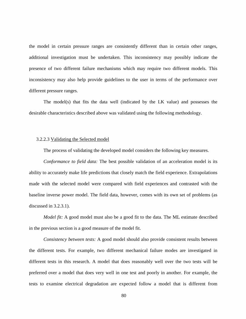
80
the model in certain pressure ranges are consistently different than in certain other ranges,
additional investigation must be undertaken. This inconsistency may possibly indicate the
presence of two different failure mechanisms which may require two different models. This
inconsistency may also help provide guidelines to the user in terms of the performance over
different pressure ranges.
The model(s) that fits the data well (indicated by the LK value) and possesses the
desirable characteristics described above was validated using the following methodology.
3.2.2.3 Validating the Selected model
The process of validating the developed model considers the following key measures.
Conformance to field data: The best possible validation of an acceleration model is its
ability to accurately make life predictions that closely match the field experience. Extrapolations
made with the selected model were compared with field experiences and contrasted with the
baseline inverse power model. The field data, however, comes with its own set of problems (as
discussed in 3.2.3.1).
Model fit: A good model must also be a good fit to the data. The ML estimate described
in the previous section is a good measure of the model fit.
Consistency between tests: A good model should also provide consistent results between
the different tests. For example, two different mechanical failure modes are investigated in
different tests in this research. A model that does reasonably well over the two tests will be
preferred over a model that does very well in one test and poorly in another. For example, the
tests to examine electrical degradation are expected follow a model that is different from

81
mechanical degradation, due to the fact that the underlying failure mechanisms for electrical
degradation and mechanical degradation are significantly different.
One of the risks in empirical models is that a model that performs well under a specific
criterion fails to perform well on another. While this may be unavoidable in certain scenarios,
this research will attempt to validate a model that performs well over a wide list of criteria
discussed above. The performance of the default IPL model over the list of criteria will also be
performed to contrast the advantages and disadvantages of the model developed.
3.2.3 Bayesian Estimation
One of the disadvantages of any statistical estimate is the uncertainty around the numbers
obtained. This uncertainty is a bigger concern in estimates from accelerated life tests using a new
model.
Bayesian methods estimate the parameters of an acceleration model by combining prior
knowledge with the parameters estimated by typical parameter estimation methods such as ML
method. The prior information may come from any number of sources including expert opinion,
physical/chemical theory, field data, and prior test data. This information is usually expressed in
the form of a prior distribution and is combined with new parameters using numerical analysis
techniques. This method presents the following advantages:
Fewer test units: By using prior information from the sources discussed above, the
parameters of the same level of precision may be obtained with much fewer test units resulting in
reduced amount of resources required to conduct the test. For example, a normal scenario which

82
requires hundreds of test units may be avoided by using Bayesian estimation to update the
existing test results on twenty or thirty units.
Less uncertainty in estimated parameters: The Bayesian method also provides a means of
improving the uncertainty in the parameters estimated. This increased level of confidence may be
required in certain mission critical applications. The distribution of parameters obtained through
Bayesian updating also reinforces the nature of the uncertainty and the subsequent reduction in
uncertainty.
Ability of ongoing updates: The Bayesian method also provides a distribution of
parameters which can be updated on an ongoing basis. For example, the posterior parameter
distributions obtained from Bayesian updating can be used as prior information in future tests to
improve the accuracy of the parameters on an ongoing basis.
Efficient use of field data: A failure reporting, analysis, and corrective action system
(FRACAS) is one of the basic requirements in any engineering organization and is often
considered a first step in the development of a reliability engineering program. Most companies
that apply accelerated life techniques can be expected to have a mature FRACAS system that
tracks the field reliability data. The wealth of information available through this venue can be put
to use using Bayesian methods. The Bayesian updating using field data also gives a sense of
assurance that the final test results are closely aligned with the field experiences.
3.2.3.1 Challenges with Field Data
Even though the field data provides tremendous leverage to improve the estimates
obtained from ALT, the data comes with its own set of problems described below.

83
Operation time: In most subsea applications, there are extensive preparatory activities
and redundancies involved. So the actual operational time of the units expected to be in service is
difficult to estimate. The units considered to be in service may either be stored as a spare in
warehouse, in a deck of an offshore platform, or subsea in a passive mode (i.e. without
transmitting power or providing the intended functions).
Failure cause: The investigations of the field failures are rather complicated. Factors like
operator intervention or unexpected field conditions may result in failure modes that could be
confounded with other failure modes. A careful review of the field conditions and root cause
analysis must first take place before including any such data.
Accurate records: Another problem with the historic field data is the accuracy and the
completeness of the records. In some cases critical pieces of information may be inaccurately
documented or missing.
Unreported failures: In some cases, failures may not be reported, either because of the
lack of monitoring capabilities subsea or customer discretion to not report failures. In such cases,
the analyst may overestimate the reliability of the product or the failure mechanism under
investigation.
All the above factors were considered before the use of field data in Bayesian estimation
methods. Despite these concerns, field data serves as a valuable resource when available. This
research used such field data and other supporting test data as input in the Bayesian estimation
approach.

84
3.2.3.2 Prior Information from Field Data
The most critical and challenging part of the Bayesian estimation process is the process
of constructing the prior distribution from the field data. Once the prior distribution is
established, the process of obtaining a posterior distribution can be accomplished by the use of
computerized mathematical calculations. In some cases the field data is not precise enough to
directly lead to the construction of a prior distribution. Additional review and expert analysis
may be required to transform the prior information from field data to meaningful prior
distributions. For example, failure data from several pressure levels may be required to construct
prior distributions on the parameters. Expert opinion may be used in some scenarios to estimate
the probabilities of different values of the parameter to be estimated. This information could lead
into the construction of appropriate prior distributions.
As described above, there are several methods of obtaining the posterior distribution, thus
the choice of the method and subsequent distribution obtained may become a key factor. It is
important to note that the choice of the prior distribution affects the final estimates, hence, a
sensitivity analysis should be performed to understand the effect of the prior distribution choice.
3.2.3.3 Bayesian Calculations
Once the prior distribution is constructed, the ML estimates may be combined with the prior
information to construct the posterior distribution. The mathematical description of Bayesian
methodology is provided below:

85
∫=
θθθθθ
θdfDataL
fDataLf)()|()()|()(
0
0 (85)
Where
θ - Vector of model parameters,
)(θf - Posterior combined distribution of model parameters,
)(0 θf - Prior combined distribution of model parameters, and
L – Likelihood function.
The individual distributions of the model parameters can then be obtained from the
posterior combined distribution. The calculations necessary for Bayesian inference require
analytic or numerical approximations. The MCMC (Markov Chain Monte Carlo) is one of the
popular methods used for achieving this approximation. The MCMC method produces
acceptable approximations to the integrals required for the Bayesian inference. This approach is
primarily used in medical applications, but recently has been adopted in the reliability
engineering applications [67] as well.
The posterior parameter distributions provide us with less uncertainty on the model
parameters and bring with them the assurance that “real” data from the field has been
incorporated into the calculations. The posterior distributions also provide us an opportunity to
choose a value from the distribution based on the confidence level required (usually by
management choice).
86
3.2.3.4 Ongoing updates
One of the key advantages of Bayesian estimation is the ability to update the distributions
of the parameters with new test data. A posterior distribution from a given test may be used as
prior information in another test. For example, in our case the posterior distributions from the
test 2 (step 1 and ramp) was used to improve the estimates from tests 2 (step 2). One must,
however, ensure that the prior information is relevant and is similar to the failure mechanism
under study.
3.3 Summary of research methodology
The research methodology for this project was illustrated in this section and the three
major sections discussed in detail. Although certain parts of the research are dependent on other
sections, the three sections are not completely sequential. There was opportunity for empirical
model fitting with preliminary results. Groundwork on Bayesian inference may also begin prior
to the actual tests. This groundwork includes review of field data and construction of prior
information. The critical path of the project was however dictated by the completion of the three
accelerated life tests.

87
CHAPTER FOUR: FINDINGS
This chapter provides an overview of the accelerated life tests conducted and the analysis
of test data including empirical model fitting, model validation, and Bayesian analysis. All
degradation values and failure times have been modified to proprietary information.
4.1 Accelerated life tests
This section reviews the three accelerated life tests that were conducted including review
of test planning, physics of failure, test results, and model fitting.
4.1.1 Test One: material properties of engineering plastics
The primary function of a mated pair of sub-sea electrical connectors is to provide means
to transfer electrical energy under sub-sea conditions. The engineering plastics used in the
connector provide several reliability critical functions, including electrical and mechanical
isolation, between key design elements and the sea water. It is, therefore, important for the
plastics to retain their material properties over time. The degradation and eventual loss of these
properties will result in complete loss of connector function. Hence the degradation of material
properties is considered a key response variable and is investigated in this test.
4.1.1.1 Test planning
The test planning process included the process of selecting the materials to be tested,
stress levels, equipment, safety review, material characteristics to be tested, number of samples

88
etc. Two engineering plastics, plastic A and plastic B, were chosen as the candidate materials due
to their wide spread use in the subsea industry. Other materials including elastomers and
ceramics were also considered. One of the materials chosen for the test is also the material from
which the component tested in Section 4.1.3 is made. This comparison provides an opportunity
to verify the degradation mechanism and the life-stress relationship at both the material level and
component level. Both of the materials are exposed to subsea pressure in applications and
understanding the effects of subsea pressure on these material properties is critical to their
reliability.
The pressure levels to be tested were selected based on industry requirements. With the
subsea applications constantly moving to deeper waters, test pressures were selected at 10 kpsi,
20 kpsi, and 30 kpsi. Three pressure levels were selected to ensure the ability to model any non-
linear pressure-life relationship. The step-stress profile used in the test is shown in Figure 12.
Figure 12: Stress profile in materials test

89
As shown in Figure 12, samples were taken out of the pressure vessel every 600 hrs to
test key material properties. Pressure was increased every 1800 hrs with testing at three pressure
levels listed.
4.1.1.2 Physics of failure
The physics of failure analysis for this test includes identifying the stress-life relationship
to be investigated, material properties to be investigated, and the effects of degradation in such
material properties. As shown in Figure 13, several stress factors including temperature,
pressure, voltage, and other mechanical stress factors affect the degradation of material
properties in engineering plastics. This test however looks at subsea pressure with temperature
held at constant room temperature. While temperature and voltage may have an interaction with
pressure in affecting the material properties, their life-stress relationships are generally accepted
and can be described with the help of the Arrhenius relationship and IPL. The effect of subsea
pressure on key material properties is however unknown and this fundamental research attempts
to investigate the sole effect of hydrostatic pressure on material properties. Understanding this
life-stress relationship is the key first step in ALT of a variety of components made from
engineering plastics in use in the subsea industry.
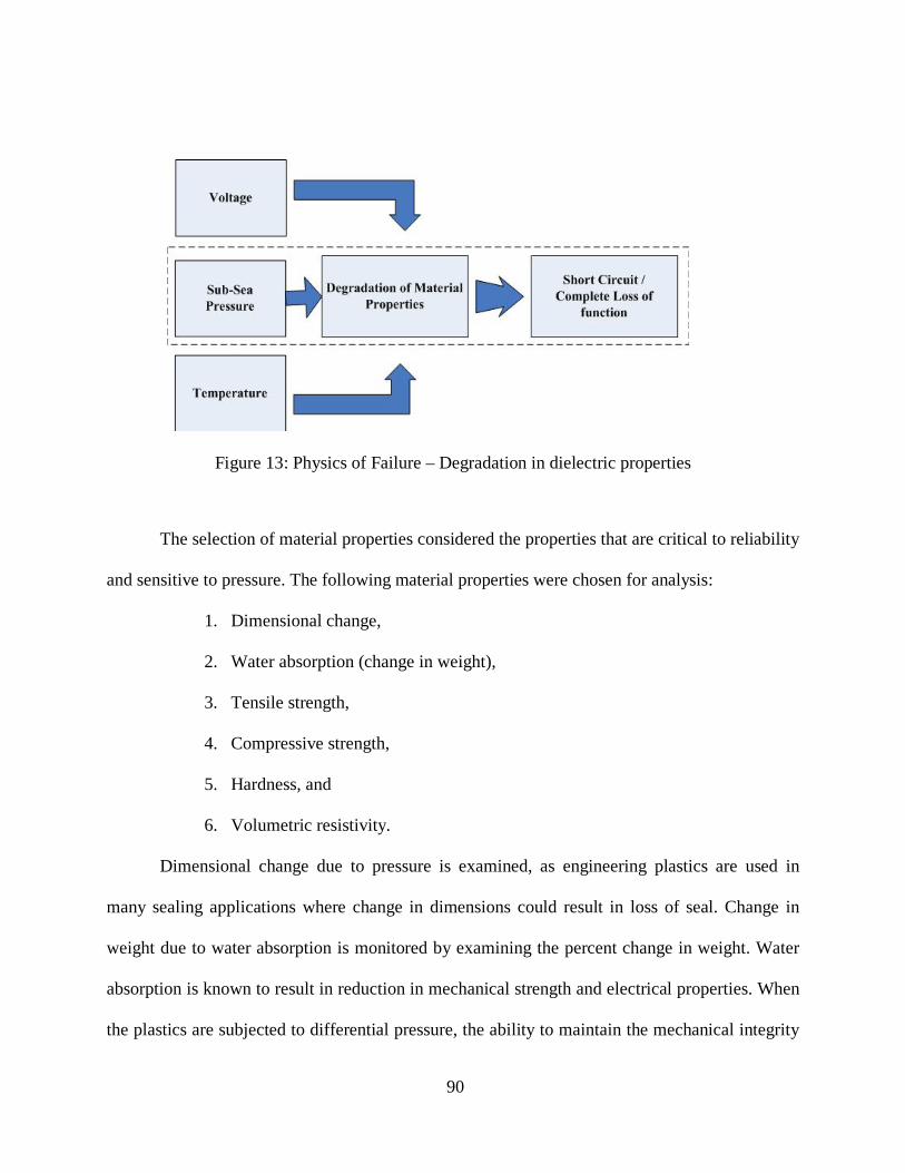
90
Figure 13: Physics of Failure – Degradation in dielectric properties
The selection of material properties considered the properties that are critical to reliability
and sensitive to pressure. The following material properties were chosen for analysis:
1. Dimensional change,
2. Water absorption (change in weight),
3. Tensile strength,
4. Compressive strength,
5. Hardness, and
6. Volumetric resistivity.
Dimensional change due to pressure is examined, as engineering plastics are used in
many sealing applications where change in dimensions could result in loss of seal. Change in
weight due to water absorption is monitored by examining the percent change in weight. Water
absorption is known to result in reduction in mechanical strength and electrical properties. When
the plastics are subjected to differential pressure, the ability to maintain the mechanical integrity

91
is dependent on key mechanical properties such as tensile strength, compressive strength, and
hardness. The general theory suggests that the resistivity of material would decline over time due
to the ingress of water molecules. This research attempts to quantitatively understand this
relationship by measuring volumetric resistivity.
4.1.1.3 Materials and equipment
All the testing was done using standard ASTM (American Standard for Testing of
Material Properties) coupons. Three type of coupons, A, B, and C, were used for the analysis. A
Type A sample is a 1” x 2” sample used for dimensional measurements (length), weight (in
accordance with ASTM D 570 for water absorption base line), volumetric resistivity (per ASTM
D-257), and SHORE "D" hardness test (ASTM-D2240). After removal from the pressure vessel,
the samples are dried off with a lint free cloth and weighed immediately (to avoid water egress).
Dimensional measurements (length, width and thickness) are then taken, followed by volumetric
resistivity (per ASTM D-257) and SHORE "D" Hardness Test (ASTM-D2240) measurements.
All the aged specimens were photographed and retained. Type B samples are “dog bone” shaped
and are used to perform destructive tensile strength tests. The tests were done per ASTM-D638.
Type C samples are cylindrical and are used to perform destructive compressive strength tests.
The tests are done per ASTM D 570. The three types of samples were machined out using water
jet cutting as shown in Figure 14.

92
Figure 14: Types of coupons used in material tests
The 30 coupons constitute the 3 measurements to be made every 600 hours. An
additional 10 samples were reserved for baseline measurements before the coupons are subjected
to pressure with additional 20 samples reserved for future research beyond 5400 hours. The
additional testing will be conducted at 6400 hrs and 7400 hrs as a part of future research. The
total number of coupons tested in entirety for the two engineering plastics under test amounts to
a total of 720 samples. Table 3 shown below provides a summary of the tests conducted and
specimens used.

93
Table 3: Summary of coupons used in materials test
All the samples were bagged in plastic bags with salt water (to simulate sea water) and
labeled with the test time at which it must be taken out of the pressure vessel and tested. The
tests were conducted in a pressure vessel that is rated to a working pressure of 30,000 psi. The
pressure vessel along with the coupons is shown in Figure 15 and Figure 16 below.
A B C A B C10 10 10 10 10 1010 10 10 10 10 1010 10 10 10 10 1010 10 10 10 10 1010 10 10 10 10 1010 10 10 10 10 1010 10 10 10 10 1010 10 10 10 10 1010 10 10 10 10 1010 10 10 10 10 1010 10 10 10 10 1010 10 10 10 10 10
120 120 120 120 120 120Total samples used
0
10000
20000
30000
0
30002400
3600
Plastic A Plastic BPressure Accumulated Time
74006400540048004200
18001200600

94
Figure 15: Pressure Vessel – Test One
Figure 16: Samples in Pressure Vessel

95
4.1.1.4 Test Results
The test results were comprised of degradation data at each pressure level, which were
then, extrapolated using a suitable degradation model to obtain time to failures at each of the
pressure levels. The time to failure was determined based on establishing a failure threshold for
the degradation characteristic being measured. This threshold is necessary in order to obtain
(through extrapolation using degradation analysis) time to failures at different pressure levels.
The failure times at different pressure levels were then used to make predictions at the use
pressure level (3000 psi). The life predictions were repeated for several models to determine the
model that best fits the data. The best fit is determined by comparing the LK value. The above
steps were repeated for each of the six material characteristics being investigated and for both
material types.
Dimensional Change (percent change): The change in dimensions is the first basic
physical property that is to be investigated. This change is a critical characteristic as some of the
components manufactured from these plastics are used for sealing functions and such changes in
dimensional features over time could lead to loss of seal and catastrophic failure. The average
change in length (dimensional change from baseline measurements) as a percentage is shown in
Table 4 below. Figure 17 and Figure 18 below show the templates used for performing
dimensional measurements and the process of taking measurements. The templates help in
performing dimensional measurements in the exact same points in the specimen.

96
Figure 17: Templates for Dimensional Measurements
Figure 18: Dimensional Measurements on Specimens

97
Table 4: Change in Length (percent) – Plastic A
10 kpsi 600 hrs 1200 hrs 1800 hrs
0.003314 0.003859 0.004891
20 kpsi 600 hrs 1200 hrs 1800 hrs
0.008288 0.010302 0.012794
30 kpsi 600 hrs 1200 hrs 1800 hrs
0.009238 0.012081 0.010899
Table 5 below shows the degradation values for tests conducted on plastic B.
Table 5: Change in Length (percent) – Plastic B
10 kpsi 600 hrs 1200 hrs 1800 hrs
0.008053 0.008292 0.009945
20 kpsi 600 hrs 1200 hrs 1800 hrs
0.014077 0.018707 0.044386
30 kpsi 600 hrs 1200 hrs 1800 hrs
0.021066 0.02214 0.02627
The failure threshold (necessary for extrapolation) for the change in length was set at 2
percent change in length, based on engineering analysis (amount of change in length that would
result in a failure such as loss of seal). Several models were evaluated for extrapolation and the
linear model proved to be most appropriate for plastic A. The exponential model proved to be the

98
best fit for plastic B. Models that do not provide a monotonic relationship (as shown in Figure 3)
were not considered. The extrapolated time to failures for both plastic A and B are shown in
Table 6 below.
Table 6: Extrapolated time to failure (2% Change in Length) – Plastic A and B
Time to Failure (hrs) Pressure Plastic A Plastic B 10 kpsi 3.09E+04 3.02E+03 20 kpsi 1.06E+04 5.49E+02 30 kpsi 8.83E+03 2.13E+03
Water absorption (change in weight): Water absorption under subsea pressure is one of the
critical parameters to be considered for reliability under subsea pressure. In most cases the
amount of water absorption leads to undesirable effects such as weakening of material properties
and electrical properties. Specimens were weighed initially for baseline measurements, after the
600 hr intervals at each pressure level; ten specimens were retrieved from the pressure vessel and
weighed after wiping of excess moisture on the surface. Figure 19 below shows a specimen
being weighed.
Figure 19: Weight Measurements on Specimens

99
The average change in weight at different time intervals and different pressure levels is
shown in Table 7 and Table 8 below.
Table 7: Change in Weight (percent) – Plastic A
10 kpsi 600 hrs 1200 hrs 1800 hrs
0.023225 0.026159 0.032194
20 kpsi 600 hrs 1200 hrs 1800 hrs
0.047032 0.049786 0.050112
30 kpsi 600 hrs 1200 hrs 1800 hrs
0.043339 0.051773 0.054104
Table 8: Change in Weight (percent) – Plastic B
10 kpsi 600 hrs 1200 hrs 1800 hrs 0.07495 0.098678 0.109637
20 kpsi 600 hrs 1200 hrs 1800 hrs
0.158621 0.161347 0.164057
30 kpsi 600 hrs 1200 hrs 1800 hrs
0.138164 0.174317 0.170297
The failure threshold (necessary for extrapolation) for the water absorption was set at 2
percent change in weight, based on engineering analysis (amount of change in weight that would
result in degradation in mechanical integrity). Several models were evaluated for extrapolation

100
and the linear model proved to be most appropriate for plastic A. Linear and power models are
chosen for plastic B. Models that do not provide a monotonic relationship were not considered.
The extrapolated time to failures for both plastic A and B are shown in Table 9 below.
Table 9: Extrapolated time to failure (2% Change in weight) – Plastic A and B
Time to Failure (hrs) Pressure Plastic A Plastic B 10 kpsi 5.11E+03 6.31E+04 20 kpsi 1.33E+04 4.09E+03 30 kpsi 2.55E+03 2.59E+03
Volumetric resistivity: It must be noted that, both engineering plastics selected for the test
are dielectric materials with good insulating properties. The change in dielectric properties over
time under subsea pressure and the rate of change at different levels of subsea pressure is of great
interest and is investigated in this research. A direct measurement of insulation resistance in
ohms is made from the specimens and is converted into volumetric resistivity based on the
volume of specimens. Specimens were tested initially for baseline measurements, after the 600
hr intervals at each pressure level; ten specimens were retrieved from the pressure vessel and
tested after wiping of excess moisture on the surface. The setup for insulation resistance
measurement is shown in Figure 20 below. The sample specimen is placed between the platens
shown Figure 21.

101
Figure 20: Equipment Setup for Insulation Resistance Measurement
Figure 21: Specimen Tested for Insulation Resistance

102
The average volumetric resistivity at different time intervals and different pressure levels for
plastic A is shown in Table 10 below.
Table 10: Volumetric Resistivity (ohm-cm) – Plastic A
10 kpsi 600 hrs 1200 hrs 1800 hrs
1.3563E+20 1.3542E+20 1.3525E+20
20 kpsi 600 hrs 1200 hrs 1800 hrs
1.4590E+19 2.4084E+18 9.5678E+17
30 kpsi 600 hrs 1200 hrs 1800 hrs
4.6458E+17 1.0905E+17 2.2745E+17
Similarly tests were conducted on plastic B, the results of which are reported in Table 11 below.
Table 11: Volumetric Resistivity (ohm-cm) – Plastic B
10 kpsi 600 hrs 1200 hrs 1800 hrs
1.5486E+20 1.5401E+20 2.4302E+18
20 kpsi 600 hrs 1200 hrs 1800 hrs
1.6149E+19 4.8959E+16 5.5690E+15
30 kpsi 600 hrs 1200 hrs 1800 hrs
7.7449E+17 1.7024E+16 5.0636E+16

103
The failure threshold (necessary for extrapolation) for volumetric resistivity was set at
3.27E+06 ohm-cm, based on engineering analysis. This threshold equates to a 50% reduction
(recommended by Underwriters Laboratory) of the log values of initial resistance. Several
models were evaluated for extrapolation and the exponential model proved to be most
appropriate for plastic A. A logarithmic model was chosen for plastic B. Models that do not
provide a monotonic relationship in degradation were not considered. The extrapolated time to
failures for both plastic A and B are shown in Table 12 below.
Table 12: Extrapolated time to failure (Volumetric Resistivity) – Plastic A and B
Time to Failure (hrs) Pressure Plastic A Plastic B 10 kpsi 4.53E+07 2.85E+20 20 kpsi 4.46E+04 1.08E+04 30 kpsi 3.61E+04 1.36E+04
Tensile strength: Tensile strength is the first of the three mechanical properties examined in
this research. Tensile strength of most materials is lower than the compressive strength , in most
real world scenarios where the applied stress is a combination of the two types (tensile and
compressive), understanding the degradation of tensile strength is important. A tensile failure in
most cases would result in a loss of mechanical integrity and a catastrophic failure. Specimens in
the shape of a dog-bone were tested under tensile stress until failure. Figure 22 below shows a
failed specimen.

104
Figure 22: Specimen under tensile strength test
The load at which the specimen breaks under tension is recorded and the tensile strength is
then derived based on the cross section of the specimen. The procedure is repeated after the
predetermined 600 hr intervals at each of the three (10 kpsi, 20 kpsi and 30 kpsi) pressure levels.
The average tensile strength values obtained for plastic A is listed in Table 13 below.
Table 13: Tensile Strength (psi) – Plastic A
10 kpsi 600 hrs 1200 hrs 1800 hrs 24751.6 23887.1 23514.7
20 kpsi 600 hrs 1200 hrs 1800 hrs 21880.5 21298.9 20818.5
30 kpsi 600 hrs 1200 hrs 1800 hrs 20019.2 19924.8 19111.8

105
Similarly tests were conducted on plastic B, the results of which are reported in Table 14 below.
Table 14: Tensile Strength (psi) – Plastic B
10 kpsi 600 hrs 1200 hrs 1800 hrs 29253.4 28687.0 28580.7
20 kpsi 600 hrs 1200 hrs 1800 hrs 28343.8 28250.0 28091.7
30 kpsi 600 hrs 1200 hrs 1800 hrs 27953.1 27465.1 25329.0
The failure threshold (necessary for extrapolation) for tensile strength was set at 50% of
the original strength (recommended by Underwriters Laboratory). This value was established as
8000 psi for plastic A and 9000 psi for plastic B. Several models were evaluated for
extrapolation and the logarithmic and linear models proved to be most appropriate for plastic A.
linear model was chosen for plastic B. Models that do not provide a monotonic decrease in
degradation were not considered. The extrapolated time to failures for both plastic A and B are
shown in Table 15 below.
Table 15: Extrapolated time to failure (Tensile Strength) – Plastic A and B
Time to Failure (hrs) Pressure Plastic A Plastic B 10 kpsi 7.37E+07 2.72E+16 20 kpsi 2.55E+07 4.39E+05 30 kpsi 6.47E+04 4.56E+04
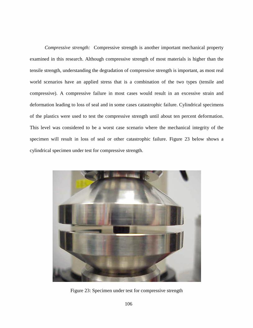
106
Compressive strength: Compressive strength is another important mechanical property
examined in this research. Although compressive strength of most materials is higher than the
tensile strength, understanding the degradation of compressive strength is important, as most real
world scenarios have an applied stress that is a combination of the two types (tensile and
compressive). A compressive failure in most cases would result in an excessive strain and
deformation leading to loss of seal and in some cases catastrophic failure. Cylindrical specimens
of the plastics were used to test the compressive strength until about ten percent deformation.
This level was considered to be a worst case scenario where the mechanical integrity of the
specimen will result in loss of seal or other catastrophic failure. Figure 23 below shows a
cylindrical specimen under test for compressive strength.
Figure 23: Specimen under test for compressive strength

107
The load at which the specimen reaches a ten percent deformation was recorded and the
compressive strength is then derived based on the cross section of the specimen subjected to the
load. The average compressive strengths obtained for plastic A are listed below in Table 16.
Table 16: Compressive Strength (psi) – Plastic A
10 kpsi 600 hrs 1200 hrs 1800 hrs 16306.3 14544.3 14643.8
20 kpsi 600 hrs 1200 hrs 1800 hrs 17256.0 15849.1 16355.7
30 kpsi 600 hrs 1200 hrs 1800 hrs 16901.1 16698.2 16964.2
Similarly tests were conducted on plastic B, the results of which are reported in Table 17 below.
Table 17: Compressive Strength (psi) – Plastic B
10 kpsi 600 hrs 1200 hrs 1800 hrs 13610.7 14263.8 12846.3
20 kpsi 600 hrs 1200 hrs 1800 hrs 14720.0 14203.9 14210.0
30 kpsi 600 hrs 1200 hrs 1800 hrs 14746.8 14644.3 13528.1

108
Difference in cross section of the two ends of the cylindrical specimen was considered by
using the average strength. The test was repeated after the predetermined 600 hr intervals at each
of the pressure levels. The failure threshold (necessary for extrapolation) for compressive
strength was set at 50% of the original strength (recommended by Underwriters Laboratory).
This value was established as 5000 psi for plastic A and plastic B. Several models were
evaluated for extrapolation and the logarithmic model proved to be most appropriate for plastic
A and plastic B. Models that do not provide a monotonic relationship in degradation were not
considered. The extrapolated time to failures for both plastic A and B are shown in Table 18
below.
Table 18: Extrapolated time to failure (Compressive Strength) – Plastic A and B
Time to Failure (hrs) Pressure Plastic A Plastic B 10 kpsi 4.71E+05 6.50E+06 20 kpsi 1.90E+07 2.77E+09 30 kpsi 5.65E+09 1.17E+06
It is important to note that, although the extrapolations lead to a monotonic function , the
life (time to failure) is shown to increase with an increase in pressure, this is counter-intuitive
and different from the trend observed in the other physical, electrical, and mechanical properties
investigated thus far in the research. This observation can, however, be justified with a proper
physics of failure investigation, which clarifies the fact that interstitial spaces in the material
which cause a low compressive strength will be reduced at higher pressures resulting in an
increase in strength.
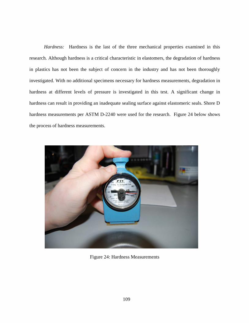
109
Hardness: Hardness is the last of the three mechanical properties examined in this
research. Although hardness is a critical characteristic in elastomers, the degradation of hardness
in plastics has not been the subject of concern in the industry and has not been thoroughly
investigated. With no additional specimens necessary for hardness measurements, degradation in
hardness at different levels of pressure is investigated in this test. A significant change in
hardness can result in providing an inadequate sealing surface against elastomeric seals. Shore D
hardness measurements per ASTM D-2240 were used for the research. Figure 24 below shows
the process of hardness measurements.
Figure 24: Hardness Measurements

110
The change in hardness values obtained for plastic A is shown in Table 19 below.
Table 19: Change in hardness (%) – Plastic A
10 kpsi 600 1200 1800
-0.0158 -0.1103 -0.1210
20 kpsi 600 1200 1800
-0.0369 -0.0211 0.0108
30 kpsi 600 1200 1800
0.0214 -0.0264 -0.1107
There are no clear trends in the above data to establish a life-stress analysis. This non-trend is
also evident in the plot shown in the Figure 25 below.
Figure 25: Trend of change in hardness values – Plastic A

111
The hardness data collected from plastic B is shown in Table 20 below.
Table 20: Change in hardness (%) – Plastic B
10 kpsi 600 hrs 1200 hrs 1800 hrs -0.0210 -0.0677 -0.0885
20 kpsi 600 hrs 1200 hrs 1800 hrs -0.0262 -0.0523 -0.0472
30 kpsi 600 hrs 1200 hrs 1800 hrs -0.0314 0.0369 -0.0578
The data from the tests on plastic B was also plotted as shown in Figure 26 below.
Figure 26: Trend of change in hardness values – Plastic B
Based on the two plots and the relevant data, it is clear that a life-stress relationship
cannot be established with the data available. Although hardness seems to decrease at lower

112
pressure levels, the hardness value decreases slowly and increases at higher pressure levels. The
test methods used in this research were investigated to understand their potential contribution to
the discrepancies observed. No shortcomings in the test methods were discovered. More testing
as a part of future research is required to establish a clear life-stress relationship.
4.1.1.5 Model Fitting
The model fitting and analysis of data includes fitting the data to the power law model
(which is the state of the art for default selection when the model is unknown) and the two
variations of the exponential model (simple exponential and inverse exponential). This will help
determine the model that is best suited to describe the pressure life relationship. It is important to
note that the Arrhenius model follows an inverse exponential form, and for most other stresses
the IPL is used. The simple exponential model, is however, not commonly used for ALT.
A ML estimate (Λ) will be used as a measure of the model fit to the test data.
),( delmoonacceleratidatatestf=Λ (86)
For failures, likelihood can be expressed by the probability density function of the
combined distribution at time it .
)....;( 1 niiii tfL γγ= (87)
Where γ1i…. γni are the parameters to be estimated.
For censored units, likelihood can be expressed as the reliability function of the combined
distribution at time it :

113
)....;(1 1 niiii tFL γγ−= (88)
It is assumed that test observations are independent. Then the likelihood, L , of having a
data set with J test observations is the combined probability of the J test outcomes:
JLLLL ...21 ××= (89)
(94) can be simplified by a log-likelihood function which is,
)ln(...)ln()ln( 21 JLLL ++=Λ (90)
The ML function will be used to estimate the required parameters β, K, and n. The
likelihood function of the IPL-Weibull model can thus be written as follows.
( ) ∑∑=
−−
=
−
=Λ
S
i
ni
nii
TKVi
ni
ni
F
ii TKVNeTKVKVN i
ni
1
'1
1)()(ln ββ
β
β (91)
The parameters of the IPL-Weibull model can be estimated by differentiating the above
equation with respect to each of these parameter estimates, equating the partial derivatives to 0,
and solving for β, K, and n using numerical methods.
0,0,0 =
∂Λ∂
=∂
Λ∂=
∂Λ∂
nand
Kβ (92)
In some cases when the model is not a good fit to the data, there are no solutions for the
parameters and a different model must be used. The higher the value of the likelihood
function (Λ), the better the fit of the model to the data. A similar process was used to
estimate fit of the exponential model and the inverse exponential model, both of which have
two parameters as well. The functional form of the exponential model is:

114
pneKpL ⋅=)( (93)
where p is pressure, L is life, and K and n are the parameters estimated from the data. The
functional form of an inverse exponential model is:
pn
eKpL =)( (94)
Table 21 shows the likelihood values and the associated mean time between failures
(MTBF) of all the material properties investigated in this research for plastics A and B. It is
important to note that the MTBF values are changed to protect confidential information. The
actual LK values are listed. The model with the best fit (highest likelihood value) is
highlighted in blue. LK value is specific to a specific data set and cannot be compared to LK
values from another data set. For example LK values of different models for tensile strength
(plastic A) can be compared but values between plastic A and B or tensile A and compressive
A cannot be compared. The MTBF values shown in the table illustrate the significance of the
model fitting to life predictions. A small change in likelihood value causes a large change in
MTBF and hence the model fit results in a significant difference in the predicted failure time.
The MTBF numbers of models that do not fit best are shown as a fraction of the best fit
MTBF. As shown in Table 21, the exponential model is a better fit for the majority of
properties examined, the inverse exponential model is a better fit for change in length, water
absorption-B, and resistivity-A. The MTBF values shown in the table illustrate the impact of
a small change in likelihood values resulting in significant differences in life estimates.

115
Table 21: Model Fitting – Likelihood Values for Material Properties
4.1.1.6 Discussion
The results from the tests show that the exponential model provides the better fit to the
data than the power relationship and inverse-exponential relationship. Further validation of the
fit of an exponential model to a pressure-life relationship was accomplished through the analysis
of results from component testing (4.1.2 and 4.1.3) including, testing of a component made from
the same material tested in this test.
4.1.2 Test Two: deformation and fracture of a plastic component
This test was conducted on the electrical connector component that acts as a physical
barrier between the two regions of differential pressure. It is to be noted that the failure of this
component will result in a catastrophic sub-sea connector.
Likelihood Value Mean Time Between Failures (hrs) Power Exp Inv Exp Power Exp Inv Exp
Dimensional-A -32.5139 -33.9807 -30.0098 4.09% 1.40% 5.12E+07
Dimensional-B -30.5186 -30.6015 -30.4333 227.78% 146.03% 6.12E+05
Water Absorption - A -34.4686 -34.4077 -34.4608 88.23% 4.56E+04 49.39% Water Absorption - B -33.1626 -34.6599 -30.5594 0.03% <0.01% 9.57E+10
Volumetric Resistivity - A -35.1825 -36.6599 -33.4200 <0.01% <0.01% 3.24E+19
Volumetric Resistivity - B -69.7357 -61.3764 -69.7357 >999% 2.14E+09 35.63% Tensile Strength - A -46.0800 -45.2402 -46.5397 30.79% 8.28E+11 >999% Tensile Strength - B -62.3834 -60.5210 -63.6167 <0.01% 7.31E+12 <0.01%
Compressive Strength - A -53.4189 -53.3489 -53.4271 78.11% 5.98E+16 7.97% Compressive Strength - B -50.348 -47.9103 -51.6330 >999% 2.40E+35 <0.01%

116
4.1.2.1 Test planning
Time varying stress profiles were used for the test to provide flexibility and ensure timely
completion of the tests. The test plan included both a step-stress profile and progressive stress
(ramp) profile. The step-stress tests were long-term tests conducted over 15,000 hours on 4 units
and the progressive stress tests were conducted on ten units to obtain failure quickly. The
progressive stress tests were conducted at a pressure (ramp) rate of 1000 psi per minute. Table 22
presents the summary of stress levels.
Table 22: Summary of stress profile – Test 2
4.1.2.2 Physics of failure
As one of the first steps in the test planning, a physics of failure model shown below was
created. The failure mode that would result in the loss of the pressure barrier function is the
No of Test Units Start Time (hrs) End Time (hrs) Pressure (psi)4 0 3000 7500
3000 4000 80004000 5000 85005000 6000 90006000 7000 95007000 15000 10000
ramp pressure(15000 – 18000)
4 0 1000 125001000 2000 130002000 3000 135003000 4000 140004000 5000 145005000 until failure 15000
10 0 to failure

117
viscoelastic strain and fracture of the component involved and is hence chosen as the response
variable. Hydrostatic pressure and temperature are the key stresses that affect this failure
mechanism, with pressure being the dominant stress factor. By maintaining the temperature at
the use level and by varying the pressure, the effect of pressure on the given failure mechanism
can be established. The typical subsea temperature is around 5oC. The typical applied current in
the electrical connector causes an 18oC rise in temperature of the component. Thus the test
temperature was established to be 23oC. Figure 27 shows the key stresses that affect the failure
mechanism.
Figure 27: Physics of failure – deformation and fracture of a plastic component

118
“Plastics exhibit viscoelastic behavior; that is, the deformation that results from an
applied load has both an elastic (immediate) and viscous (time-dependent) component.
Understanding the viscous strain rate and identifying the strain to failure are critical elements of
life prediction for plastic components subjected to long-term exposure to external loads. The
curve in Figure 28 is a typical viscoelastic stress-strain curve. The elastic behavior of the plastic
materials is relatively straightforward and can be predicted with reasonable accuracy using
conventional linear elastic analysis where the stress and strain are related by the elastic modulus.
Here the modulus is derived from short-term tests with relatively high strain rates. One method
of predicting the time dependent strain of polymers subjected to a constant stress is to use an
“apparent modulus” from isochronous stress-strain curves” [68].
Figure 28: Illustration of viscoelastic strain.
Unfortunately this data is not always readily available for engineering plastics, either it
does not exist or manufacturers are unwilling to share it, leaving the engineer to compile this

119
information on his own. Also, any available data is typically from simple specimens and can
only be used at the designer’s peril, as they will not replicate the potentially complex geometry
and/or stress state of the actual part being used in subsea conditions. As a result, long-term tests
simulating the actual part geometry and service loads will invariably yield more accurate
reliability data. Given the pressure-life relationship of the materials and the relatively complex
geometry of the parts in question it was determined that this test would be a good addition to the
research [68].
4.1.2.3 Materials and equipment
The long-term test program was designed to allow testing of four (4) of the components
simultaneously at pressures up to 10000 psi and provide temperature regulation. The temperature
of the device was estimated (including self heating due to applied current) and controlled in the
equipment. The components were populated with electrical contacts, so that electrical properties
such as insulation resistance could be monitored throughout the test. Figure 29 depicts the test
pressure vessel with the components and instrumentation installed in the end caps. The
temperature of the test vessel is to be continuously monitored. The deformation of the
component under test is continuously monitored using a transducer. The dielectric properties of
the component are also monitored continuously using a mega-ohm meter. The calibration on all
measuring equipment was verified prior to use. The test setup was also carefully designed to
ensure that the use conditions in the product are simulated. The component used for the test was
produced under the manufacturing processes used for general production. The units also went
through the preliminary tests applicable for all products to screen for infant mortality failures. A

120
test fixture which can test up to four components at a time (shown in Figure 29) was designed
and manufactured [68].
Figure 29: Test Setup – Deformation and fracture of a plastic component
A displacement indicator was positioned to make physical contact with the back of the
test component to monitor the deflection of the plastic base resulting from the applied load. The
test equipment was configured to provide a continuous record of pressure, temperature, and
deflection of each of the four components. Figure 30 and Figure 31 show the pressure vessel
used for the test and the setup of components in the pressure vessel. Failed components were
photographed and retained for records. All the failures were thoroughly examined through a
physics of failure analysis to ensure that there is no change in the underlying failure mechanism.

121
Figure 30: Setup on components in fixture
Figure 31: Fully assembled test tank

122
4.1.2.4 Test results
The first test started at 7500 psi and was suspended at 10000 psi after approximately
15000 hrs. The test profile is shown in Figure 32 below. The failure times in this case were hence
extrapolated using degradation analysis.
Figure 32: First step stress profile on test plastic component
The deformation data from the 10000 psi step was used to predict the failure times based
on a 0.02 inch failure threshold (amount of deformation that will result in fracture). Several
models were fitted to the curve but a linear model was chosen due to the lowest error (mean
square error).
The degradation data from the four components tested (A, B, C, D) are listed in Table 23.
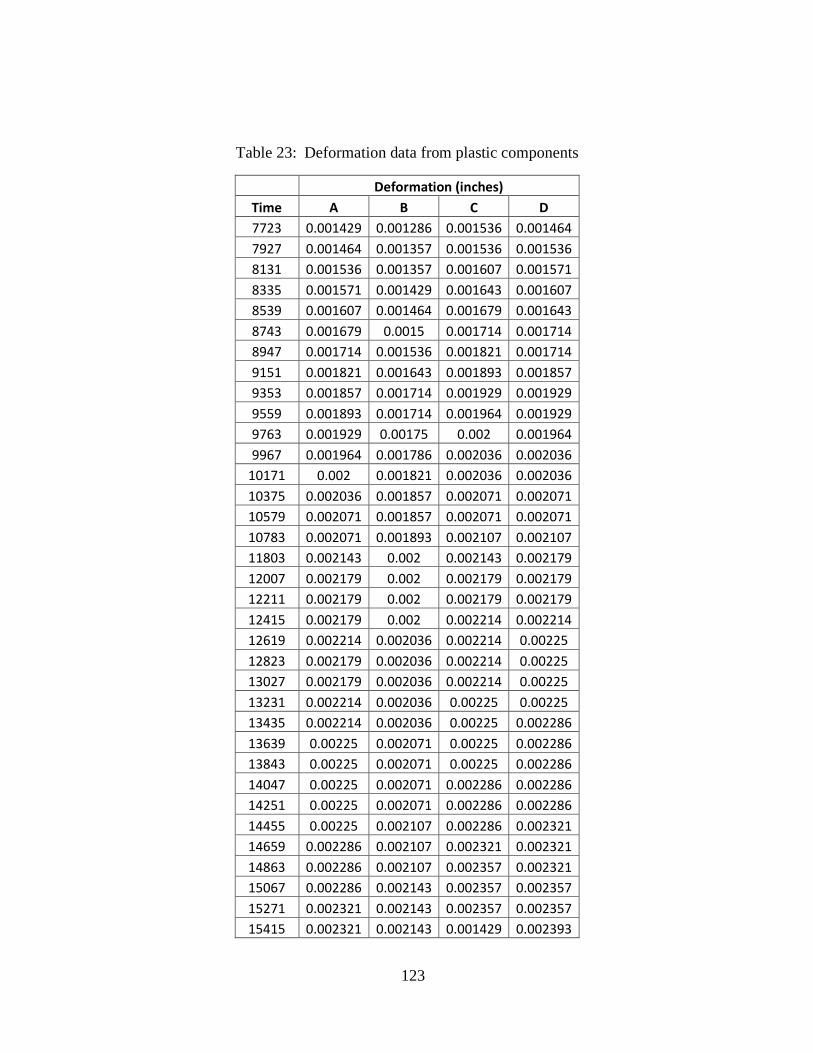
123
Table 23: Deformation data from plastic components
Deformation (inches) Time A B C D 7723 0.001429 0.001286 0.001536 0.001464 7927 0.001464 0.001357 0.001536 0.001536 8131 0.001536 0.001357 0.001607 0.001571 8335 0.001571 0.001429 0.001643 0.001607 8539 0.001607 0.001464 0.001679 0.001643 8743 0.001679 0.0015 0.001714 0.001714 8947 0.001714 0.001536 0.001821 0.001714 9151 0.001821 0.001643 0.001893 0.001857 9353 0.001857 0.001714 0.001929 0.001929 9559 0.001893 0.001714 0.001964 0.001929 9763 0.001929 0.00175 0.002 0.001964 9967 0.001964 0.001786 0.002036 0.002036
10171 0.002 0.001821 0.002036 0.002036 10375 0.002036 0.001857 0.002071 0.002071 10579 0.002071 0.001857 0.002071 0.002071 10783 0.002071 0.001893 0.002107 0.002107 11803 0.002143 0.002 0.002143 0.002179 12007 0.002179 0.002 0.002179 0.002179 12211 0.002179 0.002 0.002179 0.002179 12415 0.002179 0.002 0.002214 0.002214 12619 0.002214 0.002036 0.002214 0.00225 12823 0.002179 0.002036 0.002214 0.00225 13027 0.002179 0.002036 0.002214 0.00225 13231 0.002214 0.002036 0.00225 0.00225 13435 0.002214 0.002036 0.00225 0.002286 13639 0.00225 0.002071 0.00225 0.002286 13843 0.00225 0.002071 0.00225 0.002286 14047 0.00225 0.002071 0.002286 0.002286 14251 0.00225 0.002071 0.002286 0.002286 14455 0.00225 0.002107 0.002286 0.002321 14659 0.002286 0.002107 0.002321 0.002321 14863 0.002286 0.002107 0.002357 0.002321 15067 0.002286 0.002143 0.002357 0.002357 15271 0.002321 0.002143 0.002357 0.002357 15415 0.002321 0.002143 0.001429 0.002393

124
The extrapolation using the linear model resulted in failure times of 27426, 29979,
27129, and 26713 hrs. Figure 33 below shows the extrapolation of the degradation data for the
four components tested.
Figure 33: Extrapolation of degradation data
The next phase of tests included tests where the pressure is progressively increased until
failure. The pressure was increased at the rate of 1000 psi per minute until the component
cracked. Ten components were tested to failure in this manner. The stress profile is shown in
Figure 34. Since the long term test lasted in excess of 15000 hrs without failure, the next profile

125
was selected at a level where failures happened in a few thousand hours. Understanding the
failure pressure (15,000 – 17500 psi in a few minutes) using the progressive tests helped to
establish this new stress profile.
Figure 34: Progressive pressure profile.
The failure times in the progressive stress tests are listed in Table 24 below. In addition to
the step-stress profile discussed earlier the progressive tests helped to decide the next profile
(shown in Figure 35).

126
Table 24: Failure times and pressure in progressive pressure test
Failure Pressure (psi) Failure Time (hrs) 18378 0.3063 18420 0.3070 19356 0.3226 18858 0.3143 19561 0.3260 19644 0.3274 19380 0.3230 19450 0.3242 21205 0.3534 20850 0.3475
The third phase of the testing was conducted between 12500 psi to 15000 psi. The step
stress profile is shown in the Figure 35 below. Failures in this test profile were updated using
Bayesian analysis (4.3).
Figure 35: Second step stress profile on test - plastic component

127
4.1.2.5 Model fitting
The power model is commonly used for non-thermal stresses such as a fatigue loads and
voltage and also used as the default back-up model when the stress is not temperature (the
Arrhenius model is shown to provide a good fit for temperature) and a correct model of choice is
not known. The model fitting and analysis of data includes fitting the data to the power law
model and variations of the exponential model (simple exponential and inverse exponential). A
ML estimate (Λ) will be used as a measure of the model fit to the test data.
In some cases when the model is not a good fit to the data, there are no solutions for the
parameter and a different model must be used. The log-likelihood value of the power model,
exponential model, and the inverse exponential model are listed below in Table 25. The higher
(closer to zero) the log-likelihood value, the better the fit of the data is to the model. LK value is
specific to a specific data set and cannot be compared to LK values from another data set (test 1
vs test 2). The MTBF is also listed to show the significance of a small change in likelihood
value. With more than one value (time to failure) used at each of the stress levels, the life
distribution (Weibull and lognormal) was also considered in this case.
Table 25: Log-likelihood values of the analysis of data from plastic component ALT
Model Distribution LK Value MTBF (hrs) IPL Weibull -27.3551 >999.99% IPL Lognormal N/A N/A EXP Weibull -24.5027 2.31E+14 EXP Lognormal -22.6609 1.40E+14
INV EXP Weibull -31.013 >999.99% INV EXP Lognormal -29.3737 >999.99%
128
It must be noted that the power model is either unsolvable for an IPL-lognormal or is
lower than the exponential model in the case of a Weibull. The exponential model provides a
much better fit to the data and it is important to note that the choice of the life distribution seems
to slightly affect the likelihood values, but the impact on the MTBF value is minimal. The
inverse exponential scenario does provide a good fit to the data.
4.1.2.6 Discussion
The above results provide sufficient evidence to suggest that the exponential model
provides a much better fit to the data and to the pressure-life relationship, which is the focus of
this research. This is consistent with the results of materials test discussed in 4.1.1. Further
validation of the model was performed by comparison to test three.
4.1.3 Test Three: degradation and loss of hermetic seal
This test is similar to the previous test, but was conducted on a design feature that seals
and isolates an optical fiber from two regions under differential pressure. This test gives a
different perspective on the effect of pressure by looking at optical degradation. A sketch of the
component to be tested is shown in Figure 36 below.

129
Figure 36: Test Component – Hermetic Penetrator
4.1.3.1 Test planning
There are several variations of the component shown in Figure 36 with 4, 8, and 12
optical fibers. The test plan involves three variations of the component at the stress levels shown
below in Table 26. The performance of the three variations did not differ (beyond normal
variation within group) since the cross sectional area of the glass solder (key design feature) is
the same and hence the strength of the bond is expected to be the same.
Table 26: Stress Levels for Test 3
No of Test Units Start time (hrs) End time (hrs) Pressure (psi)
4 + 2 0 10000 13000
4 + 2 0 3500 30000
3500 5000 35000
5000 Until failure 40000

130
4.1.3.2 Physics of failure
The failure mechanism is stress cracking and rupture of the glass solder’s hermetic seal.
The resultant effect is a loss of optical circuit. This effect is usually preceded by optical
degradation (increase of optical loss). The physics of failure model shown in Figure 37 for this
test was developed to show the underlying failure mechanism.
Figure 37: Physics of failure – loss of hermetic seal
Similar to the failure mechanisms in the previous test, temperature and pressure are the
variables that affect the failure mode. Pressure is the dominant variable to be investigated in the
research. As shown in the model, the preliminary effect is on the epoxy seal which physically
precedes the hermetic seal. Any degradation in optical performance due to the effect of pressure
on epoxy is to be monitored.
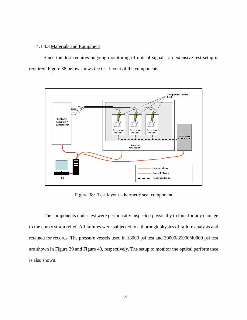
131
4.1.3.3 Materials and Equipment
Since this test requires ongoing monitoring of optical signals, an extensive test setup is
required. Figure 38 below shows the test layout of the components.
Figure 38: Test layout – hermetic seal component
The components under test were periodically inspected physically to look for any damage
to the epoxy strain relief. All failures were subjected to a thorough physics of failure analysis and
retained for records. The pressure vessels used in 13000 psi test and 30000/35000/40000 psi test
are shown in Figure 39 and Figure 40, respectively. The setup to monitor the optical performance
is also shown.

132
Figure 39: 13000 psi pressure vessel
Figure 40: 30-40 kpsi pressure vessel

133
4.1.3.4 Test Results
All the results from the test are degradation type data, which are then extrapolated to the
failure threshold to obtain failure times. The degradation data from the 13 kpsi test is shown in
Table 27 below.
Table 27: Degradation Data at 13 kpsi
Time Optical Loss (dB) (hrs) Unit 1 Unit 2 Unit 3 Unit 4 Unit 5 Unit 6
1 1.3000 1.7072 0.4523 0.7047 0.8610 1.6860 336 1.3115 1.6908 0.4450 0.7100 0.8420 1.6611 672 1.3173 1.6863 0.4430 0.7112 0.8411 1.6551
1008 1.3238 1.6878 0.4435 0.7100 0.8487 1.6618 1344 1.3248 1.6842 0.4334 0.7071 0.8551 1.6552 1680 1.3244 1.6837 0.4317 0.7071 0.8612 1.6523 2016 1.5199 1.6926 0.4355 0.7065 0.8998 1.6509 2352 1.5247 1.6852 0.4345 0.7012 0.7657 1.5634 2688 1.5749 1.6852 0.4348 0.7053 0.7748 1.5481 3024 1.9600 1.6889 0.4404 0.7100 0.7740 1.5477 3360 2.7902 1.7116 0.4520 0.7365 0.7829 1.5573 3696 2.4038 1.6870 0.4325 0.7088 0.7668 1.5317 4032 1.1827 1.6252 0.3862 0.6929 0.7916 1.5327 4368 2.0913 1.6837 0.4320 0.6976 0.7679 1.5178 4704 1.9864 1.6738 0.4330 0.6988 0.7713 1.5192 5040 1.9216 1.6759 0.4321 0.6994 0.7746 1.5190 5376 1.8528 1.6716 0.4323 0.6971 0.7721 1.5105 5712 1.1827 1.6252 0.3862 0.6929 0.7916 1.5327 6048 1.8184 1.6519 0.4310 0.6665 0.7911 1.4968 6384 1.8175 1.6525 0.4277 0.6653 0.7942 1.4869 6720 1.8239 1.6438 0.4277 0.6659 0.7943 1.4830 7056 1.8151 1.6524 0.4269 0.6600 0.8269 1.4769 7392 1.8173 1.6476 0.4246 0.6641 0.8375 1.4747 7728 1.8291 1.6512 0.4295 0.6624 0.8555 1.4780 8736 1.8294 1.6477 0.4299 0.6588 0.8840 1.4725 9072 1.8340 1.6476 0.4304 0.6582 0.8884 1.4728 9408 1.8384 1.6481 0.4310 0.6576 0.8897 1.4723
9744 1.8398 1.6531 0.4325 0.6512 0.8788 1.4724

134
In this test, the optical failure threshold is set as 10 dB of optical loss, which essentially
equates to the inability of an optical fiber to transmit data. From the degradation data it is clear
that apart from Unit 1, all other units have decreasing optical loss (increasing performance).
These 5 units are considered as suspensions until the 3.00+E12 hrs. (highest failure time from
other units in the test). For Unit 1, the degradation trend best fits a power relationship and
extrapolation to 10dB was obtained as 2.95+E12 hours.
Next degradation data from the 30 kpsi test for the first 3500 hrs are examined. As
discussed in test planning, the pressure was increased to 35 kpsi after 3500 hrs. The optical loss
data is shown in Table 28 and Table 29.
Table 28: Degradation Data at 30 kpsi – Part A
Time Optical Loss (dB) (hrs) Unit 1 Unit 2 Unit 3 Unit 4 Unit 5 Unit 6
1 0.0359 0.0569 0.3052 0.2265 0.1841 0.1430 98 0.1018 0.5987 0.5414 0.4147 0.2829 0.2749
196 0.0838 0.7022 0.5393 0.4075 0.3246 0.2770 294 0.1162 0.8318 0.5513 0.4091 0.3245 0.2729 392 0.3765 0.8688 0.5421 0.4053 0.3199 0.2661 490 0.7224 0.8843 0.5326 0.3993 0.3129 0.2663 588 1.2453 0.8931 0.5220 0.3898 0.3052 0.2606 686 2.0235 0.8940 0.5171 0.3846 0.3015 0.2645 784 2.6247 0.8869 0.5040 0.3868 0.3030 0.2548 882 3.1738 0.8974 0.4954 0.3814 0.2934 0.2455 980 9.9862 0.9049 0.5098 0.3746 0.2888 0.2407
1078 10.9891 0.9091 0.4985 0.3686 0.2829 0.2353 1176 10.7841 0.9156 0.4923 0.3652 0.2800 0.2327 1274 13.2826 0.9207 0.4843 0.3625 0.2762 0.2256 1372 21.8665 0.9238 0.4781 0.3592 0.2721 0.2280 1470 19.6885 0.9257 0.4701 0.3518 0.2668 0.2225 1568 29.4553 0.9369 0.4662 0.3490 0.2631 0.2218 1666 33.2979 0.9415 0.4612 0.3458 0.2591 0.2188

135
Table 29: Degradation Data at 30 kpsi – Part B
Time Optical Loss (dB) (hrs) Unit 1 Unit 2 Unit 3 Unit 4 Unit 5 Unit 6 1764 34.33529 1.066324 0.453039 0.337059 0.254706 0.216667 1862 40.51029 2.888382 0.448235 0.334118 0.252157 0.21402 1960 42.85588 1.451912 0.447255 0.33402 0.251667 0.213824 2058 46.85294 1.564265 0.443529 0.329412 0.248039 0.213235 2156 51.51235 1.662941 0.442843 0.324706 0.246863 0.211471 2254 51.50882 1.761912 0.436569 0.321863 0.243627 0.21902 2352 42.60176 1.810441 0.446961 0.323627 0.246667 0.215784 2450 47.76677 1.886029 0.430294 0.316471 0.239118 0.215294 2548 51.4947 1.997206 0.424314 0.315392 0.238922 0.199216 2646 51.49235 2.168676 0.420294 0.312157 0.236863 0.202745 2744 42.69147 2.292353 0.416373 0.308627 0.236078 0.203137 2842 42.73412 2.415147 0.413137 0.30402 0.241471 0.197745 2940 41.01618 2.469559 0.36402 0.296569 0.233235 0.201078 3038 44.23853 2.600588 0.358333 0.293039 0.231176 0.199804 3136 43.76941 2.775588 0.354118 0.286961 0.22902 0.201667 3234 45.74059 2.895441 0.349216 0.283235 0.227941 0.197647 3332 46.93147 2.878676 0.345098 0.276275 0.225098 0.196863 3404 47.42441 2.7625 0.343922 0.273529 0.226863 0.197941
As seen in the degradation data, Unit 1 fails during the test (exceeds 10 dB). This was
calculated as 980 hrs (no extrapolation is required). Unit 2 shows degradation during the test, and
a linear model was identified as the best fit model. Extrapolation to 10 dB was estimated at 7836
hours. The other 4 units, as seen in the data, do not see any degradation but see improvement in
optical loss. Similar to the 13 kpsi data, these units will be considered as suspensions at
3.00+12hrs.
After increasing the pressure to 35 kpsi, the test was suspended after a few hundred hours
of degradation data was obtained. The unit 1 that already failed at 30kpsi test before the pressure

136
was increased to 35 kpsi. The rest of the 5 units will be monitored in this step. The degradation
data from the 400 hrs at 35kpsi is shown in Table 30.
Table 30: Degradation Data at 35 kpsi
Time Optical Loss (dB) (hrs) Unit 1 Unit 2 Unit 3 Unit 4 Unit 5 Unit 6
1 N/A 2.7625 0.3439 0.2735 0.2269 0.1979 98 N/A 5.4891 0.4014 0.2622 0.3722 0.2319
196 N/A 9.7629 0.3997 0.2624 0.3675 0.2305 294 N/A 12.0138 0.3973 0.2443 0.3983 0.2307 392 N/A 13.5816 0.3947 0.2458 0.4185 0.2288
Unit 2 failed in the first 107 hours (cumulative 3607 hours including time at 30 kpsi). Unit 4
showed increasing performance and will be considered a suspension at 3.00+12hrs. Units 3, 5
and 6 were extrapolated using linear and exponential models to obtain failure times (hrs) of
13761, 16908, and 14948 respectively.
4.1.3.5 Model Fitting
The data from the three stress levels (13 kpsi, 30 kpsi, and 35 kpsi) were analyzed to identify the
best fit model. With several units under test, the life distribution at each stress level was
identified. Table 31 shown below lists the likelihood values for the power, exponential and
inverse exponential models.
The table also shows the likelihood values for both Weibull and log-normal life distributions
The likelihood values for the simple exponential model were closest to zero indicating the best
fit among the candidate models. The inverse exponential model is the second best fit. In both

137
cases the lognormal life distribution appears a better fit than Weibull model. The power model
appears to be the worst fit and the solution for power-lognormal model could not be obtained due
to a poor fit.
Table 31: Likelihood Values and MTBF for Test 3
Model Distribution LK Value MTBF (hrs) IPL Weibull -113.2101 >999%
IPL Lognormal N/A N/A EXP Weibull -112.7777 3.13E+37 EXP Lognormal -111.3339 6.94E+37
INV EXP Weibull -113.2101 >999%
INV EXP Lognormal -112.6483 >999%
4.1.3.6 Discussion
The results from test three further corroborate the fit of the exponential model to describe
the pressure-life relationship. This is consistent with results from tests one and two. A proper
validation of the model will now be performed based on criteria established in research
methodology.
4.2 Model validation
The model validation process primarily involves comparison of the data from the three
independent tests and to field data. The characteristics of the model of choice in a variety of
scenarios are also examined.

138
4.2.1 Validation by comparison between tests
We have examined the data from the three tests for model fit individually and found the
simple exponential model to have a good fit to the failure data in most cases. Now we compare
the results of model fit among the three tests in Table 32 below.
Table 32: Rank of Model Fits of Three Tests
The simple exponential model is the clear choice for the mechanical properties at the
material level (tensile and compressive strength) and also for the component level failures
(mechanical) in Test 2 and 3. This information provides us reasonable evidence to suggest the
exponential model is a good fit of the pressure-life relationship for mechanical failure modes.
The exponential model is also a good fit for the water absorption mechanism, which can affect
Power Exp Inv ExpMaterial Tests
Dimensional - A 2 3 1Dimensional - B 2 3 1Water Absorbtion - A 2 1 3Water Absorbtion - B 2 3 1Volumetric Resistivity - A 3 2 1Volumetric Resistivity - B 2 1 2Tensile Strength - A 2 1 3Tensile Strength - B 2 1 3Compressive Strength - A 2 1 3Compressive Strength - B 2 1 3
Component TestDeformation/Fracture 3 1 2
Component TestLoss of Hermetic Seal 3 1 2
Test 3
Model Fit Rank
Test 1
Test 2
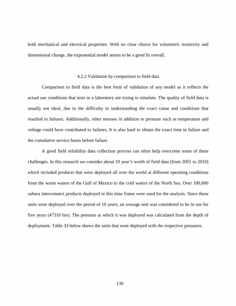
139
both mechanical and electrical properties. With no clear choice for volumetric resistivity and
dimensional change, the exponential model seems to be a good fit overall.
4.2.2 Validation by comparison to field data
Comparison to field data is the best form of validation of any model as it reflects the
actual use conditions that tests in a laboratory are trying to simulate. The quality of field data is
usually not ideal, due to the difficulty in understanding the exact cause and conditions that
resulted in failures. Additionally, other stresses in addition to pressure such as temperature and
voltage could have contributed to failures. It is also hard to obtain the exact time to failure and
the cumulative service hours before failure.
A good field reliability data collection process can often help overcome some of these
challenges. In this research we consider about 10 year’s worth of field data (from 2001 to 2010)
which included products that were deployed all over the world at different operating conditions
from the warm waters of the Gulf of Mexico to the cold waters of the North Sea. Over 100,000
subsea interconnect products deployed in this time frame were used for the analysis. Since these
units were deployed over the period of 10 years, an average unit was considered to be in use for
five years (47310 hrs). The pressure at which it was deployed was calculated from the depth of
deployment. Table 33 below shows the units that were deployed with the respective pressures.

140
Table 33: Deployment Information on Fielded Units
Failure data on the fielded units consisted of several types of failure from mechanical
failures, to electrical failures, optical failures. Only mechanical failures where pressure is the
dominant stress in the failure mechanism were considered for the analysis. Table 34 below
shows information on failures. The nature of failures included loss of seals and other mechanical
failure modes such as crushed and ruptured components. This choice is consistent with other
mechanisms investigated in this research.
Table 34: Failure Information on Fielded Units
Pressure (psi) Time to Failure (hrs) 3791 9751 3791 18482 3347 52632 2902 4447 2458 4243 2458 30617 1569 6140 1569 52124 1125 46743 1125 145044
Units Pressure (psi) Service Time (hrs)2253 3791 437103195 3347 437108328 2902 43710
16153 2458 4371010749 2014 4371011799 1569 4371025867 1125 4371015091 681 4371019364 236 43710

141
Similar to the analysis of accelerated life test data the likelihood values were used to
measure the fit of the data to the model. The MTBF values are also shown in Table 35 below to
illustrate the effect of a small change in likelihood values. No solution was obtained for an IPL-
Weibull model.
Table 35: Likelihood Values from Field Data
Model Distribution LK Value MTBF (hrs) IPL Weibull N/A N/A IPL Lognormal -211.17 <0.01% EXP Weibull -205.27 5.22E+10 EXP Lognormal -205.02 4.32E+19
INV EXP Weibull -205.44 87.30% INV EXP Lognormal -205.20 115.75%
The exponential model has the better fit to the data than the inverse exponential and
inverse power models. For a given life distribution (Weibull), we see that the exponential model
(-205.27) has a higher (closer to zero) likelihood value than inverse exponential (-205.44). A
similar observation is made for lognormal scenario. This observation further confirms that the
exponential model is best suited to describe the pressure-life relationship for mechanical failures.
4.2.3 Characteristics of Simple Exponential Model
There are several characteristics of the simple exponential model that make it the model
of choice to describe the pressure-life relationship.
Simplicity of the model: The exponential model is a simple model with only two
parameters that need to be estimated from the data. This simplicity is very desirable, as similar
models like the Arrhenius model have been preferred against more complex models including

142
the Eyring model just to minimize estimation of additional parameters. More parameters in the
model also mean that more data points are needed for estimation and could prove to be expensive
in certain accelerated life tests with high cost.
Conversion to linear scale: Another desirable characteristic that the exponential model
possesses is the ability to be converted to a linear scale. This form makes it easy to present the
results in a graphical format in a plot. The actual parameters can also be estimated graphically,
although, the ML method is still the preferred method even in case of the exponential model. The
appeal of the ML method stems from the fact that it can be applied to a wide variety of models
(both linear and/non-linear) and kinds of data (exact failures, censored and interval) where other
methods such as least squares are in general not satisfactory.
Applicability over a wider pressure range: The exponential model also holds true for a
wider range of pressure ranges. This research has thus far covered pressures from field data with
shallow water deployments with pressure on the order of a few hundred psi to the high pressure
penetrators tests as high as 35 kpsi. The exponential model has been shown to be a good fit
throughout this range. Figure 41 illustrates the pressure ranges in the various tests in the research
and field data.

143
Figure 41: Range of Pressures in the Research
Materials and Components: It is important for a good acceleration model to be
applicable for different types of materials. In this research, we have seen that not only does the
exponential model hold true for both the materials in Test 1, but it also is a good fit in Test 3
where the component is comprised of a hermetic and epoxy seal. Also, the model is a good fit at
the material level (plastic B in Test 1) as well as at the component level (component made from
plastic B in Test 2).
Failure Mechanisms: The model also appears to be appropriate for a variety of failure
mechanisms including physical (water absorption Test 1) , mechanical (tensile strength/
compressive strength – Test 1 , deformation/fracture of plastic component – Test 2) electrical
(volumetric resistivity – Test 1), and optical (optical loss – Test 3). This consistency is highly
desirable in an acceleration model. It must also be noted that several real world scenarios involve
a combination of these failure mechanisms.
144
Step-Stress and Progressive Stress Profiles: The main advantage of ALT is their ability
to significantly shorten the time required to complete the tests. In ALT where units are tested at
constant higher stresses, completing the tests in a reasonable amount of time continues to be a
problem. This problem is mainly due to the inability to estimate the stress level at which the
failure mechanism would be significantly accelerated without changing the underlying failure
mechanism. Step stress testing helps to solve this problem by providing the flexibility needed to
change the stress level during the test and hence to obtain the failures in a reasonable amount of
time. It is important for a good acceleration model to be a good fit in these step stress profile
tests. In this research, all three tests used some form of step stress profile and the exponential
model proved to be a good fit in all cases. Test 2 also included a test with progressively
increasing stress.
Effect of Units of Measure: The stress variable in a life-stress relationship may have
many units of measure. It is desirable for the acceleration model to work at these different units
of measure. For example, for the Arrhenius model to work, the temperature needs to be
converted into degrees Kelvin. Using Fahrenheit as the unit of measure for temperature may
result in incorrect predictions in an ALT analysis. For pressure, this research uses pounds per
square inch (psi) as the unit of measure. This unit is the most popular unit used in the United
States. We also examined the performance of the model for the unit measure “bar” which is
commonly accepted in the European Union. The conversion between the two is shown in the
equation below.
barpsi 0689.01 = (95)

145
The common unit Pascal can also be expressed as a different order of magnitude of bar.
Looking at the likelihood values shown in Table 36 below, we see that the exponential model
continues to be a good fit for the pressure-life relationship using either psi or bar as units of
measure for pressure. LK value is specific to a specific data set (exp-psi vs power-psi) and
cannot be compared to LK values from another data set (psi vs. bar). The data analyzed is from
the results of Test 3.
Table 36: Likelihood values for different units of measure
Effect of failure thresholds: All three tests in this research used some kind of degradation
analysis that used a failure threshold. It is important to examine the applicability of the fit of the
exponential model when these failure thresholds change. This variation will also help simulate
the effect of testing other materials or components with different geometry that may not fail at
the threshold selected. For illustration we look at the tensile strength tests on plastic B in the first
test. The initial estimates used a 50% reduction in initial tensile strength (recommended by
Underwriters Laboratory). We now look at the extrapolated time to failures if the failure
threshold is 25% and 75%. The revised time to failures are listed in Table 37 below.
Psi BarEXP -113.4016 -110.7403213
Inv EXP -114.4062 -112.5289402Power -113.7987 -111.3798958

146
Table 37: Time to failures at different thresholds
Threshold (% of original strength) 50% 25% 75%
10K 6.61E+15 3.52E+29 6.19E+07 20K 1.07E+05 1.68E+05 4.47E+04 30K 2.75E+04 4.35E+04 1.15E+04
The analysis was repeated for the new time to failures to estimate likelihood values.
Table 38 shows the fit of the three models for the different thresholds. The exponential model
continues to be a good fit for all the scenarios.
Table 38: Likelihood values at different thresholds
These eight characteristics in addition to the validation from the tests and the field data
indicate that the exponential model is best suited for the pressure-life relationship.
4.3 Bayesian Analysis
Bayesian methods are closely related to likelihood methods. Bayesian methods are used
to estimate the parameters of an acceleration model by combining prior knowledge with the
parameters estimated by typical parameter estimation methods such as ML method. This method
is especially beneficial in models used in new applications (such as the use of exponential model
50% 25% 75%Exp -62.7194 -98.1731 -33.80
Power -64.2042 -99.4786 -38.17Inv Exp -68.2564 -100.458 -40.03
Likelihood Values

147
for subsea applications), as the prior information can be used to bolster the results and prediction
using the model. This information provides increased confidence in the results and reduces many
uncertainties that exist with the use of a model in a new application.
For our pressure-life relationship shown below there are two parameters, K and n. In
addition, there is a parameter for the life distribution (β for Weibull distribution). Bayesian
analysis requires prior information on these parameters in the form of a distribution:
pneKpL ⋅=)( (96)
The prior distributions for the parameters β, K, and n can be computed using the variance
estimated from the Fisher matrix as discussed in section 2.3.3.2. An example of the Fisher matrix
is shown below (the diagonal elements have the variances of the parameters).
1
2
222
2
2
22
22
2
2
)ˆ()ˆ,ˆ()ˆ,ˆ()ˆ,ˆ()ˆ()ˆ,ˆ()ˆ,ˆ()ˆ,ˆ()ˆ(
−
∂Λ∂
−∂∂Λ∂
−∂∂Λ∂
−
∂∂Λ∂
−∂
Λ∂−
∂∂Λ∂
−
∂∂Λ∂
−∂∂Λ∂
−∂
Λ∂−
=
nKnn
nKKK
nK
nVarKnCovnCovnKCovKVarKCovnCovKCovVar
β
β
βββ
ββ
βββ
(97)
The resultant prior distribution is hence a normal prior distribution. The prior information
may come from a variety of sources including field data, prior tests, and expert judgment. In this
research, both field reliability data and data from accelerated life tests are used for sources of
prior distributions.

148
The posterior combined distribution is then computed as follows:
∫ ∫ ∫ ⋅
⋅=
K n
dKdndnKfnKDataLnKfDatanKL
β
βββββ),,(),,|(
),,(|),,(
0
0 (98)
Given the prior distribution with mean 0µ and standard deviation 0σ and new information
with normal distribution 1µ and 1σ , the posterior distribution with mean 'µ and standard
deviation 'σ can be computed using the following formulae.
121
20
21
021
20
20' µ
σσσ
µσσ
σµ
++
+= (99)
21
20
11'
σσ
σ
+
= (100)
The field data used in Section 4.2.2 can be used to construct a prior distribution and can
be used to update the parameters of Test 2 where one of the components was tested. The
estimated parameters of the posterior distribution are shown in Table 39 below.
Table 39: Bayesian Analysis using Field Data
The effect of Bayesian updating can be shown graphically in Figure 42, Figure 43, and Figure 44
below.
Mean Var Mean Var Mean VarB 0.770749 5.9E-02 0.4481 1.17E-02 0.717747 9.74E-03K 25.26021 22.5 39.62917 17.87752 31.62347 9.960496n 0.001266 3.5E-07 0.002667 8.12E-08 0.001529 6.59E-08
Prior - Field New - Test 2 Posterior
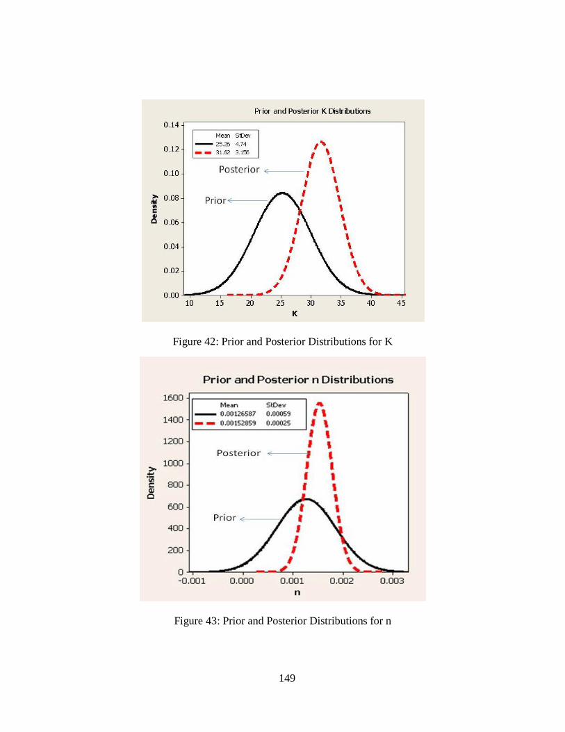
149
Figure 42: Prior and Posterior Distributions for K
Figure 43: Prior and Posterior Distributions for n
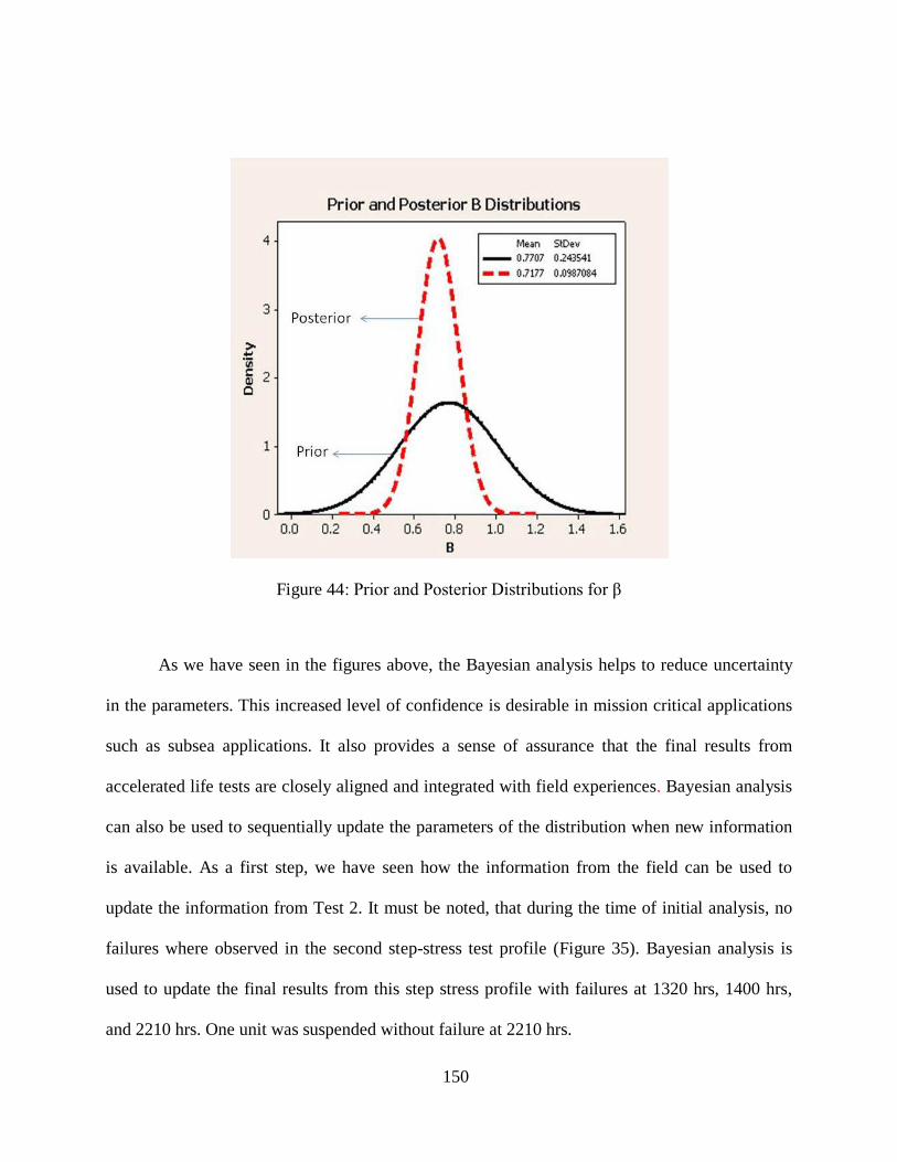
150
Figure 44: Prior and Posterior Distributions for β
As we have seen in the figures above, the Bayesian analysis helps to reduce uncertainty
in the parameters. This increased level of confidence is desirable in mission critical applications
such as subsea applications. It also provides a sense of assurance that the final results from
accelerated life tests are closely aligned and integrated with field experiences. Bayesian analysis
can also be used to sequentially update the parameters of the distribution when new information
is available. As a first step, we have seen how the information from the field can be used to
update the information from Test 2. It must be noted, that during the time of initial analysis, no
failures where observed in the second step-stress test profile (Figure 35). Bayesian analysis is
used to update the final results from this step stress profile with failures at 1320 hrs, 1400 hrs,
and 2210 hrs. One unit was suspended without failure at 2210 hrs.

151
The posterior distribution from the previous step (field data combined with test 2) is now
the prior distribution (prior 2), with new information (step 2) from the second step profile, a new
posterior distribution (posterior2) with distribution parameters (normal mean and variance) were
calculated using the formulae shown earlier. The results of the sequential Bayesian updating are
shown in Table 40 below.
Table 40: Sequential Bayesian Updating using Additional Test Data
It is important to note that the Bayesian update has resulted in a significant change in the
Weibull shape parameter (B) (0.7177 to 0.0097). In such occasions, the users must proceed with
caution, and a careful review of the new information and prior information must be completed.
In this case one of the potential causes of the significant difference in the Weibull parameter
estimate may be due to the fact that new B was based on 3 failures (and 1 suspension), whereas
the prior was based on about 24 failures (several thousand suspensions). A sensitivity analysis to
understand the impact of such a change would also be useful. Figure 45, Figure 46, and Figure
47 below show the effect of sequential Bayesian updates with the original prior 1 (field data) and
prior 2 (field and test 2) and the final posterior distribution (field, test 2, and step 2).
Mean Var Mean Var Mean VarB 0.7177 0.0097 1.7933 2.9642 1.7898 9.71E-03K 31.6235 9.9605 36.0950 12.6165 34.1223 5.5661n 0.0015 0.0000 0.0022 7.43E-06 0.0022 6.54E-08
Prior 2 New - Step 2 Posterior 2

152
Figure 45: Sequential Bayesian Updating – K distributions
Figure 46: Sequential Bayesian Updating – n distributions

153
Figure 47: Sequential Bayesian Updating – B distributions
As discussed, before the significant change in the estimate of B is clear in the Figure 47.
The sensitivity analysis to understand the impact of such a change is shown in Table 41 below.
The analysis looks at the different BX values (X indicates time for X% of units to fail) and the
mean. Before the use of new B, such information from the sensitivity analysis must be
considered.
Table 41: Sensitivity Analysis – Impact of Change in B (Weibull Shape Parameter)
(in hrs) B = 0.7177 B = 1.7898 B01 2.52E+09 4.30E+09 B10 6.63E+10 1.60E+10 B50 9.15E+11 4.59E+10
Mean 1.89E+12 5.00E+10 B90 4.88E+12 8.96E+10

154
A similar approach could be taken to update the results of the analysis with any future
research done on this failure mechanism. Thus Bayesian statistical methods help establish a
distribution of parameters which can be updated on an ongoing basis. Another key advantage of
the use of Bayesian methods in this research is the ability to obtain the same level of precision
with much fewer test units resulting in a reduced amount of resources and cost required to
conduct the test. A good example is the use of data from over 100,000 units in the field to
augment the results from a few units from the accelerated test. This information provides a level
of confidence in the results that is unobtainable through any stand-alone test results obtained
from the ML method. For instance, the critical information of interest in subsea application is the
reliability of the product during a 25 year life. In Table 42, the reliabilities of the component in a
25 year life at 3000 psi are listed. A two sided confidence interval around the reliability values is
provided as reference. The table also shows the effect of the integration of prior information into
the test data.
Table 42: Upper and Lower 95% Confidence Limits on 25 year Reliability
Figure 48 below illustrates this point in a graphical form, as shown in the figure the
confidence (especially the 95% lower confidence limit) around the predicted results has
improved significantly. In a real world scenario, this difference could mean that a significant
Test Data Posterior DataL 95% 0.99296447 0.99501477R(25) 0.99982693 0.99997459U95% 0.99999576 0.99999998

155
amount of design changes or mitigation activities can be avoided with this narrower confidence
zone.
Figure 48: Sequential Bayesian Updating – B distributions
Bayesian analysis thus complements this research by providing additional support to the
results from the proposed simple exponential model in accelerated life testing of subsea
equipment under subsea pressure.
PosteriorTest
1.000
0.999
0.998
0.997
0.996
0.995
0.994
0.993
25 y
ear
Rel
iabi
lity
at 3
000
psi
Comparison of 95% Confidence Intervals

156
CHAPTER FIVE: CONCLUSIONS AND FUTURE RESEARCH
This dissertation has for the first time proposed the exponential model (with
comprehensive validation) to describe the pressure-life relationship used in acceleration models
for life testing. Although identifying the life distribution was not the primary goal of the
research, the lognormal distribution best described the variation between units at any stress level.
This choice can vary depending on the type of design or products used.
Three independent accelerated tests were conducted and their results analyzed to identify
the best model for the pressure-life relationship. The testing included material tests in standard
coupons to investigate the effect of subsea pressure on key physical, mechanical, and electrical
properties. Tests were also conducted at the component level on critical components that
function as a pressure barrier. By comparing the likelihood values of multiple reasonable
candidate models for the individual tests, the exponential model was identified as a good model
for the pressure-life relationship. In addition to consistently providing good fit among the three
tests, the exponential model was also consistent with field data (validation with over 10 years of
field data) and demonstrated several characteristics that enable robust life predictions in a variety
of scenarios. In addition, the research also used the process of Bayesian analysis to incorporate
prior information from field and test data to bolster the results and increase the confidence in the
predictions from the proposed model. The key benefits and limitations of the proposed model are
discussed in this section. In addition, as with any other research, there are several opportunities
for future research some of which are discussed as part of the research conclusions.

157
5.1 Benefits of the Research
The contributions of the research are expected to go beyond improving the accelerated life
methodologies for subsea equipment under subsea pressure.
The acceleration model will serve as an effective design tool in developing new designs that
can survive in harsher environments. The model will also result in a better understanding of the
stresses experienced by the product during its life-time and will help engineers design products
that are suitable for new applications. Without this crucial knowledge, products are usually
“over-designed” beyond the necessary requirements resulting in expensive products and and/or
even worse with products that are “under-designed” that do not meet the requirements of the
applications. The new model will hence help develop cost-effective new designs and prevent
expensive redesigns.
Manufacturing tests / ESS: The results of the research will also enable development of better
tests to screen for manufacturing defects (infant mortality defects). Such tests are currently
conducted at arbitrary (some set at a conservative level by industry standards) levels of pressure
and time intervals. Refinements will result in more effective and efficient tests. A big fraction of
the catastrophic field failures are caused due to such shortcomings in manufacturing. Without the
application of acceleration of such manufacturing tests, the benefits of the model will be limited
to identifying and improving limitations inherent in the design.
Other similar applications: Such a model could also be useful in other applications where
hydrostatic pressure is a key variable such as civil engineering structures (e.g. bridges), on-shore
pipe-lines etc. However it is important to note that this is an empirical model and use of such a
model in other applications should be validated through empirical evidence.

158
Awareness on acceleration models: The results of the research are also expected to increase
the awareness on the use of acceleration models. The results will emphasize the need for
development of empirical models where there is a lack of complete knowledge of physical
theory. It is important to prevent such shortcomings from hampering the use of an acceleration
model with adequate empirical evidence. This evidence however does not preclude the necessary
physics of failure investigation needed for accelerated life tests. On the other end, it must also be
noted that a mathematical model such as IPL does not become an empirical model unless its
sufficiency is proven through tests. The results of this research will create an increased
awareness on this key pitfall in the use of acceleration models.
Use of Bayesian methods: The research also promotes the use of Bayesian methods to
augment the accelerated test data with expert opinion and field data and also provides a means to
continuously improve the accuracy of the estimates through ongoing Bayesian updates. This
methodology also requires the organization to have an established process for accelerated life
tests further increasing the use and benefits of accelerated life tests.
Use of statistics as an engineering tool: The research is also intended to promote the use of
statistics as an engineering tool. The unique nature of the research requires the use of both
statistical and engineering methods and hence the success and contributions of the project should
encourage engineers to use statistics as an effective tool in other engineering applications. Other
engineering applications of benefit include further research in acceleration models including
acceleration models for other stresses and multi-stress models.

159
5.2 Limitations of the Research
As with any research, one must be wary of the limitations of the research and take them into
consideration during their application in practical engineering scenarios.
Failure mechanisms: Although the proposed model is shown to work well in a variety of
scenarios, a proper physics of failure study must be done before its use in any new applications.
This is a necessary step in any accelerated test. This study may find that although a given failure
mode happens under subsea conditions, it will not be accelerated by subsea pressure. Other stress
factors like temperature, voltage and mechanical variables may be the dominant variable in such
a mechanism. The findings may also reveal scenarios where there are multiple failure
mechanisms that occur sequentially to lead to a failure mode. If the rates of degradation in these
distinct failure mechanisms are different, they would require two separate exponential models to
model the time to failure. Using one model to approximate the relationship will lead-to
inaccurate results. A similar scenario exists for an elastic-plastic failure where two power models
are required to adequately model the failure scenario. This scenario also emphasizes the
existence of several competing failure mechanisms in any given product. While using this model
in an accelerated life test, one must bear in mind that the results only apply to the failure
mechanism under investigation and no inference can be made about the overall reliability of the
product. Several accelerated life tests must be conducted on the key high risk failure mechanisms
before any inferences can be made on the product reliability. Analysis such as reliability block
diagrams is used to integrate the results from different accelerated life tests.
It must be noted that even though the model is shown to work for mechanical, physical,
electrical, and optical failure modes, further validation may be required before wide spread use

160
especially in electrical and optical failure mechanisms where there is a dearth of field data for
validation. There may also be situations where certain mechanical/physical failure modes have a
weak or inconsistent relationship with subsea pressure. In this research such a relationship was
observed for hardness. Establishing a pressure-life relationship requires a monotonic
relationship. Such a relationship could not be established for hardness, so life predictions or
model fitting was not done for this scenario.
Use stress profiles: The use stress profile of the component/product under test must be taken
into consideration. The proposed model would only apply for scenarios where the
product/component is subject to constant pressure conditions. For example, the model would not
apply to a situation where the component experiences pressure cycles throughout its life and not
constant pressure. Such a profile usually exerts higher stress on the part and predictions with the
proposed exponential model will be inaccurate. It is important to note the difference between use
stress profile and a test stress profile. A constant use stress profile can be simulated by a non-
constant profile (step-stress or ramp) in an accelerated life test, using the cumulative damage
modeling methods; however, a non-constant profile (cyclic) cannot be simulated by a constant
profile. Similar limitations exist for other acceleration models as well. A good example is the
Arrhenius relationship which has been proven to be a good fit to describe the temperature-life
relationship in a wide variety of scenarios. However, in situations where the temperature is not
constant but cyclic, the Arrhenius relationship is no longer a good fit. The IPL model is
considered a good fit to describe situations with cyclic temperature stresses.

161
5.3 Future Research
The future research in this area mainly focuses on opportunities for developing other models
for failure mechanisms that are not adequately described by the proposed simple exponential
model and expanding the research to a two-stress model to include other common subsea stresses
like temperature. Established models such as the Arrhenius model exist for these variables;
however, their interaction with the subsea pressure has not been quantified or modeled. This
research is crucial as the real world scenario almost always includes more than one stress
variable.
As an example, let us consider another variation of the exponential model, the
exponential-power model as shown below. This model may be suitable for other failure
mechanisms not supported by the simple exponential model:
,)(
nPeKpL = (101)
To estimate the fit of the model to a given set of data the following procedure should be
followed. Let us consider accelerated test data with F failures and for an exponential-power with
Weibull distribution. This combined distribution has the following form:
β
ββ
⋅−−
⋅⋅=
nP
nneK
t
PPe
eKt
eKVtf
1
),(
(102)
The ML function will be used to estimate the required parameters β, K, and n. The
likelihood function of the exponential-power-Weibull model can thus be written as follows,
where the higher the likelihood value, the better fit of the data to the model:

162
.ln1
1
⋅⋅=Λ
⋅−−
=∑
β
ββ nP
nneK
t
PP
F
ii e
eKt
eKN
(103)
First the parameters in the above likelihood function must be estimated. The parameters
of the exponential-power-Weibull model can be estimated by differentiating the above equation
with respect to each of these parameter estimates, and equating the partial derivatives to 0 (as
shown in equation 109) thus solving for β, K, and n using numerical methods.
0,0,0 =
∂Λ∂
=∂
Λ∂=
∂Λ∂
nand
Kβ (104)
The second aspect of the future research involves investigating a two-stress acceleration
model that involves subsea pressure. Temperature is the obvious choice for the second variable
of this mode due to its importance under subsea conditions. In order to achieve this next step,
combinations of pressure and temperatures must be tested. For example with temperatures values
T1 and T2 and pressure values P1 and P2 , four (T1 P1, T1 P2, T2 P1 and T2 P2) combinations
are possible. At least three of the four combinations (as shown in Table 43) must be tested for a
two-stress model.
Table 43: Stress Combinations for Two-Stress Model Development
Pressure (kpsi) Temperature (deg C)15 2315 12015 150
19.5 150

163
As a part of the future research, testing on plastic A (from test one) is being conducted at
the stress combinations listed in Table 44. Let us now consider preliminary results from water
absorption tests on plastic A. The following time to failures shown in Table 44 were obtained
after extrapolation of degradation data. A logarithmic model was good fit for extrapolation.
Table 44: Stress Combinations for Two-Stress Model Development
Pressure (kpsi) Temperature (deg C) Failure Time (hrs) 15 120 2.12E+10 15 120 2.25E+10 15 120 3.61E+10 15 150 1.31E+09 15 150 1.36E+09 15 150 1.40E+09 15 150 5.27E+09 15 150 5.54E+09 15 150 5.59E+09
19.5 150 6.30E+09 19.5 150 6.89E+09 19.5 150 7.86E+09 15 23 1.14E+19 15 23 2.14E+19 15 23 8.17E+19
The degradation tests were much shorter (200 to 800 hours) due to expensive resources
and safety concerns of tests at such high temperatures. A model fitting analysis with likelihood
values was performed on the data above. The exponential model continues to be a good model in
this scenario with slightly lower likelihood values than inverse exponential and power model as
shown in Table 45. The difference in MTBF values also shows the impact of this difference in
likelihood values.

164
Table 45: Likelihood Values for Two Stress Model
Pressure Model Temperature Model LK Value MTBF (hrs)
EXP Arrhenius -64.14290941 8.62E+14
Inv Exp Arrhenius -64.14290942 2.00E+10
Power Arrhenius -64.14290942 2.09E+14
A pressure-temperature model is shown in the equation below, where K, n, A, and m are
parameters to be estimated:
.),( tm
pn eAeKtpL ⋅= ⋅
(105)
It is important to note that these are preliminary results. Validation with other plastics and
other physical, mechanical, and electrical properties are planned. The research is also to be
extended to a three stress model including voltage and also to other materials such as elastomers
and ceramics. As emphasized earlier, such research with multi-stress situations is important due
to the nature of practical applications which experience a multi stress scenario in all cases. The
acceleration model proposed in this research for subsea pressure is an important first step
towards this goal.
165
LIST OF REFERENCES
[1] Wayne Nelson, Accelerated testing: statistical models, test plans and data analyses,
Wiley, 2004.
[2] Bryan Dodson and Harry Schwab, Accelerated Testing: A Practitioner's Guide to
Accelerated and Reliability Testing, SAE, 2006.
[3] William Q. Meeker and Luis A. Escobar, Statistical Methods for Reliability Data.
Wiley,1998.
[4] Hu, J.M.; Barker, D.B.; Dasgupta, A.; Arora, A.K., "Role of failure-mechanism
identification in accelerated testing," Reliability and Maintainability Symposium,
1992. Proceedings., Annual, vol., no., pp.181-188, 21-23 Jan 1992.
[5] Sharon Honecker, QALT Boot Camp, Reliasoft Corporation, 2008.
[6] Paul A. Tobias and David C. Trindade, Applied Reliability, Chapman & Hall/CRC,
1995.
[7] M.Modarres, ENRE 641 Accelerated Testing Course Notes, University of Maryland, 2008.
[8] Vilijandas Bagdonavicius and Mikhail Nikulin, Acceleration Life Models.
Modeling and Statistical Analysis, Chapman & Hall/CRC,2001.
[9] Lam, C.F.; Huairui Guo; Larson, L., "Time-Varying Multi-Stress ALT for Modeling Life
of Outdoor Optical Products," Reliability and Maintainability Symposium, 2007.
RAMS '07. Annual, vol., no., pp.265-270, 22-25 Jan. 2007.
[10] Swain, G., "Accelerated Testing of Antifouling Coatings for Use on Offshore
Structures," OCEANS, vol.18, no., pp. 221-226, Sep 1986.

166
[11] Park, C.; Padgett, W.J., "Stochastic degradation models with several accelerating
variables," Reliability, IEEE Transactions on, vol.55, no.2, pp. 379-390, June 2006.
[12] Tebbi, O.; Guerin, F.; Dumon, B., "Statistical analysis of accelerated experiment in
mechanics using a mechanical accelerated life model," Reliability and
Maintainability Symposium, 2003. Annual, vol., no., pp. 124-131, 2003.
[13] Tebbi, O.; Guerin, F.; Dumon, B., "Comparative study of accelerated testing models,
applications In mechanics," Systems, Man, and Cybernetics, 2001 IEEE International
Conference on, vol.4, no., pp.2099-2104 vol.4, 2001.
[14] Guerin, F.; Dumon, B.; Hambli, R.; Tebbi, O., "Accelerated testing based on a
mechanical-damage model," Reliability and Maintainability Symposium, 2001.
Proceedings. Annual, vol., no., pp.372-376, 2001
[15] Park, C.; Padgett, W.J., "New cumulative damage models for failure using stochastic
processes as initial damage," Reliability, IEEE Transactions on , vol.54, no.3, pp. 530-540,
Sept. 2005.
[16] Rosenbaum, E.; King, J.C.; Chenming Hu, "Accelerated testing of SiO2 reliability,"
Electron Devices, IEEE Transactions on, vol.43, no.1, pp.70-80, Jan 1996.
[17] Malucci, R.D., "Accelerated testing of tin-plated copper alloy contacts," Components and
Packaging Technologies, IEEE Transactions on [see also Components, Packaging and
Manufacturing Technology, Part A: Packaging Technologies, IEEE Transactions on],
vol.22, no.1, pp.53-60, Mar 1999.
[18] Lall, P.; Islam, M.N.; Singh, N.; Suhling, J.C.; Darveaux, R., "Model for BGA and CSP
reliability in automotive underhood applications," Components and Packaging

167
Technologies, IEEE Transactions on [see also Components, Packaging and Manufacturing
Technology, Part A: Packaging Technologies, IEEE Transactions on] , vol.27, no.3, pp.
585-593, Sept. 2004.
[19] Wolfgang Neher, "New Accelerating Test Methods for Board Level Solder Joints and
Thermal Caused Failure Mechanisms in High Temperature Electronics," Electronics
System integration Technology Conference, 2006. 1st, vol.1, no., pp.180-186, Sept.
2006.
[20] Setty, K.; Subbarayan, G.; Luu Nguyen, "Powercycling Reliability, Failure Analysis and
Acceleration Factors of Pb Free Solder Joints," Electronic Components and Technology
Conference, 2005. Proceedings. 55th, vol., no., pp.907-915, 0-0 0.
[21] Dokmeci, M.R.; von Arx, J.A.; Najafi, K., "Accelerated testing of anodically bonded glass-
silicon packages in salt water," Solid State Sensors and Actuators, 1997. TRANSDUCERS
'97 Chicago, 1997 International Conference on, vol.1, no., pp.283-286 vol.1, 16-19 Jun
1997.
[22] Misra, R.B., "Reliability assessment for static electricity meters," Metering and Tariffs for
Energy Supply, 1999. Ninth International Conference on (Conf. Publ. No. 462), vol., no.,
pp.151-155, Aug 1999.
[23] Eriksson, P.; Carlsson, B.; Wallinder, I.O., "Design of accelerated corrosion tests for
electronic components in automotive applications," Components and Packaging
Technologies, IEEE Transactions on [see also Components, Packaging and Manufacturing
Technology, Part A: Packaging Technologies, IEEE Transactions on], vol.24, no.1,
pp.99-107, Mar 2001.

168
[24] C. Bunea and T.A. Mazzuchi, Competing failure modes in accelerated life testing, Journal
of Statistical Planning and Inference Volume 136, Issue 5, , Competing Risks: Theory
and Applications, 1 May 2006, Pages 1608-1620.
[25] Zhao, Wenbiao & Elsayed, E. A. (2005). Modeling accelerated life testing based on mean
residual life. International Journal of Systems Science, 36 (11), 689-696.
[26] Gang Zheng and Sangun Park, Another look at life testing, Journal of Statistical Planning
and Inference Volume 127, Issues 1-2,, 1 January 2005, Pages 103-117.
[27] Ceci, C.; Mazliak, L. Optimal design in nonparametric life testing. Stat. Inference Stoch.
Process. 7 (2004), no. 3, 305--325. 62G05 (62N05 93E20).
[28] Vilijandas Bagdonavicius, Olga Cheminade and Mikhail Nikulin, Statistical planning and
inference in accelerated life testing using the CHSS model, Journal of Statistical Planning
and Inference Volume 126, Issue 2, , 1 December 2004, Pages 535-551.
[29] Gang Zheng and Sangun Park, A note on time savings in censored life testing, Journal
of Statistical Planning and Inference Volume 124, Issue 2, 1 September 2004, Pages 289-
300.
[30] J. Rene Van Dorp and Thomas A. Mazzuchi, A general Bayes exponential inference model
for accelerated life testing, Journal of Statistical Planning and Inference Volume 119,
Issue 1, , 15 January 2004, Pages 55-74.
[31] Dharmadhikari, A. D.; Rahman, Md. Monsur A model for step-stress accelerated life
testing. Naval Res. Logist. 50 (2003), no. 8, 841--868.
[32] Pascual, Francis & Montepiedra, Grace (2002). On Minimax designs when there are two
candidate models. Journal of Statistical Computation and Simulation, 72 (11), 841-862.

169
[33] Shyur, Huan-Jyh; Elsayed, E. A.; Luxhøj, James T. A general hazard regression model for
accelerated life testing. Reliability and maintenance in production control. Ann. Oper. Res.
91 (1999), 263--280.
[34] Bordes, Laurent Semi parametric additive accelerated life models. Scand. J. Statist. 26
(1999), no. 3, 345--361.
[35] Shyur, Huan-Jyh; Elsayed, E. A.; Luxhøj, James T. A general model for accelerated life
testing with time-dependent covariates. Naval Res. Logist. 46 (1999), no. 3, 303--321.
[36] Tang, L. C.; Goh, T. N.; Sun, Y. S.; Ong, H. L. Planning accelerated life tests for censored
two-parameter exponential distributions. Naval Res. Logist. 46 (1999), no. 2, 169--186.
[37] Devarajan, Karthik; Ebrahimi, Nader A nonparametric approach to accelerated life testing
under multiple stresses. Naval Res. Logist. 45 (1998), no. 6, 629--644.
[38] Abdel-Ghaly, A.A., Attia, A.F. & Aly, H.M. (1998). Estimation of the parameters of pareto
distribution and the reliability function using accelerated life testing with censoring.
Communications in Statistics - Simulation and Computation, 27 (2), 469-484.
[39] Vilijandas Bagdonavicius and Mikhail Nikulin, Accelerated life testing when a process of
production is unstable, Statistics & Probability Letters Volume 35, Issue 3, 15 October
1997, Pages 269-275.
[40] Woods, Jonathan Michael (2003) Accelerated testing for bond reliability of fiber-reinforced
polymers (FRP) to concrete and steel in aggressive environments. Ph.D. dissertation, The
University of Arizona, United States - Arizona.
[41] Wu, Changfu (2003) A new methodology in accelerated testing of mechanical heart valve
prostheses. Ph.D. dissertation, Florida Atlantic University, United States - Florida.

170
[42] Kuraishi, Akira (2001) Durability analysis of composite structures using the accelerated
testing methodology. Ph.D. dissertation, Stanford University, United States -- California.
[43] Pinnangudi, Balasubramanian (2007) A new approach for condition assessment of
polymeric housing materials used in nonceramic insulators. Ph.D. dissertation, Arizona
State University, United States -- Arizona.
[44] Gosavi, Mridula (2007) Reliability testing and modeling of linear image sensor devices.
M.S. dissertation, State University of New York at Binghamton, United States -- New
York.
[45] Qi, Haiyu (2006) Plastic ball grid array (PBGA) solder joint reliability assessment under
combined thermal cycling and vibration loading conditions. Ph.D. dissertation, University
of Maryland, College Park, United States -- Maryland.
[46] Worms, Tanya (2005) Accelerated laboratory evaluation of joint sealants under cyclic
loads. M.Sc. dissertation, University of Manitoba (Canada), Canada.
[47] Li, Qishan (2002) Accelerated degradation test planning and optimization. Ph.D.
dissertation, The University of Arizona, United States – Arizona.
[48] Sepehrifar, Mohammad B. (2006) Modeling and characterizations of new notions in life
testing with statistical applications. Ph.D. dissertation, University of Central Florida,
United States -- Florida.
[49] Rodriguez, Ivan (2007) Bayesian analysis for Cox's proportional hazard model with error
effect and applications to Accelerated Life Testing data. M.S. dissertation, The University
of Texas at El Paso, United States – Texas.

171
[50] Xie, Qihao (2006) Exact inference for exponential step-stress model under different forms
of censoring. Ph.D. dissertation, McMaster University (Canada), Canada.
[51] Gudipati, Venkata Sesha Sai Arvind (2005) Effects of missing data in competing risks on
accelerated life testing. M.S. dissertation, The University of Texas at El Paso, United States
-- Texas.
[52] Batres, Juan (2005) Integrating field failure data and accelerated life testing by Bayesian
methods for product reliability inference. M.S. dissertation, The University of Texas at El
Paso, United States -- Texas.
[53] Zhao, Wenbiao (2003) Modeling and planning accelerated life testing based on mean
residual life. Ph.D. dissertation, Rutgers The State University of New Jersey - New
Brunswick, United States -- New Jersey.
[54] Al-Haj Ebrahem, Mohammed (2003) Nonparametric accelerated degradation models in life-
testing. Ph.D. dissertation, Kansas State University, United States – Kansas.
[55] Zhang, Yao (2002) Bayesian design for life tests and accelerated life tests. Ph.D.
dissertation, Iowa State University, United States -- Iowa.
[56] Ng, Hon Keung Tony (2002) Contributions to parametric and nonparametric inference in
life testing. Ph.D. dissertation, McMaster University (Canada), Canada.
[57] Wang, Xindong (2001) An extended hazard regression model for accelerated life testing
with time varying coefficients. Ph.D. dissertation, Rutgers The State University of New
Jersey - New Brunswick, United States -- New Jersey.

172
[58] Jiao, Lixia (2001) Optimal allocations of stress levels and test units in accelerated life tests.
Ph.D. dissertation, Rutgers The State University of New Jersey - New Brunswick, United
States -- New Jersey.
[59] Sen, Debaraj (1999) Accelerated life testing: Concepts and models. M.Sc. dissertation,
Concordia University (Canada), Canada.
[60] Alhadeed, Abdulla Ahmed (1998) Models for step-stress accelerated life testing. Ph.D.
dissertation, Kansas State University, United States -- Kansas.
[61] Mahmoud Yousef, Raja Nassar, Analysis of accelerated failure times of rehabilitation liners
subjected to a constant or variable pressure, Tunnelling and Underground Space
Technology Volume 21, Issue 1, , January 2006, Pages 97-105.
[62] L.M Connelly and N Zettlemoyer, Hydrostatic effects on the capacity of DT tubular joints,
23rd Annual Offshore Technology Conference, Houston, Texas,1991.
[63] S.Y.Hanna, W.H.Thomason, J.G.Wiliams. Influence of tension, weight and hydrostatic
pressure on deepwater TLP tendons, 19th Annual Offshore Technology Conference,
Houston, Texas, 1987.
[64] V.A.Avakov, J.C.Foster, and E.J.Smith, Coiled Tubing Life Prediction, 25th Annual
Offshore Technology Conference, Houston, Texas, 1993.
[65] Lonsdale, D.; Flewitt, P. E. J, The Effect of Hydrostatic Pressure on the Uniaxial Creep
Life of a 21/4% Cr 1% Mo Steel, Proceedings of the Royal Society of London.
Series A, Mathematical and Physical Sciences Vol.373 Issue.1755, Jan. 7, 1981 Pages
491-509.
[66] MRC Biostatistics Unit, “The WinBUGS Project”, Cambridge, UK.

173
[67] Mohammadreza Azarkhail and Mohammad Modarres, Markov Chain Simulation for
estimating accelerated life parameters. Reliability and Maintainability Symposium, 2005.
Proceedings. Annual, vol., no., pp.252-257, 2005.
[68] Development of Acceleration Model for Subsea Pressure. Reliability and Maintainability
Symposium, 2010. Proceedings. Annual, vol., no., pp. 1 - 6, 2005.