1

Accepted by Cement and Concrete Composites, 2015, doi: 10.1016/j.cemconcomp.2015.10.014.

Numerical simulation of heat and mass transport during hydration of Portland

cement mortar in semi-adiabatic and steam curing conditions

E.Hernandez-Bautista 1,2*, D. P. Bentz2, S. Sandoval-Torres1, P. F. de J. Cano-Barrita1 1. Instituto Politecnico Nacional/CIIDIR Unidad Oaxaca, Hornos 1003, Oaxaca, Mexico. 71230.

2. National Institute of Standards and Technology, Gaithersburg, MD, USA. *Corresponding author: ehernandezb0800@alumno.ipn.mx

Abstract A model that describes hydration and heat-mass transport in Portland cement mortar during steam

curing was developed. The hydration reactions are described by a maturity function that uses the

equivalent age concept, coupled to a heat and mass balance. The thermal conductivity and specific

heat of mortar with water-to-cement mass ratio of 0.30 was measured during hydration, using the

Transient Plane Source method. The parameters for the maturity equation and the activation energy

were obtained by isothermal calorimetry at 23 ºC and 38 ºC. Steam curing and semi-adiabatic

experiments were carried out to obtain the temperature evolution and moisture profiles were

assessed by magnetic resonance imaging. Three specimen geometries were simulated and the

results were compared with experimental data. Comparisons of temperature had maximum residuals

of 2.5 °C and 5 °C for semi-adiabatic and steam curing conditions, respectively. The model

correctly predicts the evaporable water distribution obtained by magnetic resonance imaging.

Keywords: Accelerated curing; cement-based materials; moisture distribution; exothermic reaction;

isothermal calorimetry; nuclear magnetic resonance

1. Introduction

Steam curing of hydraulic concrete in the precast industry has the advantage of accelerating the

hydration reactions of cement. Consequently, the material develops compressive strength and

reduces its permeability in hours, compared to standard curing under normal environmental

conditions, where the hydration reactions may require several days or even months to reach an

adequate level [1].

The process of steam curing consists of increasing the temperature within a saturated water vapor

atmosphere. In this process, the cement hydration has a significant impact on the temperature

development inside the material at early ages [2] and also affects the mechanical and durability

properties of the hardened material. Therefore, it is essential to take into account the hydration

properties and temperature development to prevent premature damage to concrete.

Studies related to steam curing of concrete have been oriented toward the development of

compressive strength [3–6], pore structure development [7–9] and energetic efficiency of this

process [5,10].

In order to understand the mechanisms of heat and mass transport coupled with cement hydration,

various models have been developed to explain these phenomena [11–17]. However, these are

typically for ambient environmental conditions, therefore it is necessary to focus on hydration at

elevated temperatures and high relative humidity encountered in steam curing. Additionally, the

calculated degree of hydration varies with temperature during the curing cycle. This is of interest to

2

the precast industry. With the aims of improving curing schedules, establishing appropriate curing

conditions, improving mechanical properties and durability of cement-based materials and

obtaining a better energy efficiency in the process, this paper investigates the numerical simulation

of this curing process.

Specifically, the aim of this work is to model the hydration, moisture distribution and heat transport

during the semi–adiabatic curing of cement paste and mortar specimens so that pre-cast operations

can be optimized with respect to curing (cycle) time and energy efficiency. Nuclear magnetic

resonance (NMR) and magnetic resonance imaging (MRI) measurements are performed to

nondestructively obtain experimental evidence of the moisture distribution in small mortar

specimens to validate the model predictions.

2. Experimental procedures

2.1 Materials

The cement used in the mortar specimens was a Mexican cement designated as CPO30RS. The

oxide composition measured by X-ray fluorescence is shown in Table 1. The corresponding

potential Bogue phase composition, heat of hydration and water necessary for cement hydration

were calculated. The latter two sets of values were obtained by multiplying the Bogue mass

fractions by the accepted value for each phase as taken from the literature.

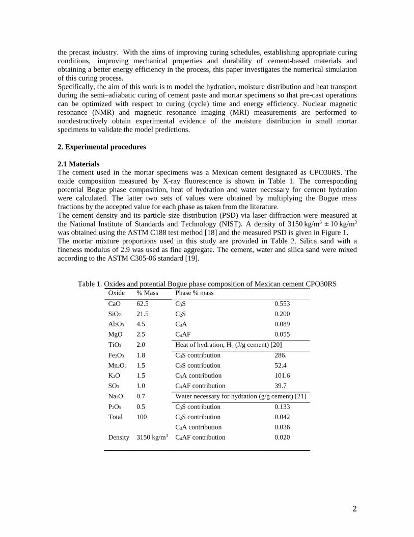
The cement density and its particle size distribution (PSD) via laser diffraction were measured at

the National Institute of Standards and Technology (NIST). A density of 3150 kg/m3 ± 10 kg/m3

was obtained using the ASTM C188 test method [18] and the measured PSD is given in Figure 1.

The mortar mixture proportions used in this study are provided in Table 2. Silica sand with a

fineness modulus of 2.9 was used as fine aggregate. The cement, water and silica sand were mixed

according to the ASTM C305-06 standard [19].

Table 1. Oxides and potential Bogue phase composition of Mexican cement CPO30RS

Oxide % Mass Phase % mass

CaO 62.5 C3S 0.553

SiO2 21.5 C2S 0.200

Al2O3 4.5 C3A 0.089

MgO 2.5 C4AF 0.055

TiO2 2.0 Heat of hydration, Hu (J/g cement) [20]

Fe2O3 1.8 C3S contribution 286.

Mn2O3 1.5 C2S contribution 52.4

K2O 1.5 C3A contribution 101.6

SO3 1.0 C4AF contribution 39.7

Na2O 0.7 Water necessary for hydration (g/g cement) [21]

P2O5 0.5 C3S contribution 0.133

Total 100 C2S contribution 0.042

C3A contribution 0.036

Density 3150 kg/m3 C4AF contribution 0.020

3

Figure 1. Cumulative and differential PSD of the cement CPO 30RS.

Table 2. Mortar mixture proportions (w/c = 0.30)

Material Proportion, kg/m3 Mass fraction

CPO30RS cement 647.81 0.271

Water 194.34 0.081

Silica sand (Dry) 1548.00 0.648

Computed Density 2390.16

2.2 Method

2.2.1 Thermal property changes during cement hydration

2.2.1.1 Heat capacity

The Transient Plane Source (TPS) method uses a sensor that consists of a combined heat source and

a resistance thermometer [22]. A constant power is supplied to the sensor for a specified period of

time and the temperature is continuously measured. The thermal properties of the sample are

calculated by analyzing the temperature development in the sensor.

For cement and dry silica sand, the heat capacity was measured using a Hot Disk Thermal Constant

Analyzer with a heat capacity unit, consisting of a probe attached to the base of a gold pan/lid. For

these measurements, the gold pan and its lid were insulated with polystyrene to prevent heat loss.

First, a reference measurement with the empty pan was made, followed by measurements with the

specimen placed in the pan. A power of 0.1 W was applied for a measurement time of 80 s [23]. For

the quantitative analysis, the acquired data points in the range of 100 to 200 out of 200 total data

points were used. Knowing the mass of the specimen, the heat capacity for each material was

calculated in J/(kg∙K). The average values are shown in Table 3, along with the standard deviations

from replicate measurements.

4

Table 3. Heat capacity of the materials

Material Cp [J/(kg·K)] Standard

deviation

[J/(kg·K)]

Cement powder 722.5 6.1

Silica sand 635.3 2.8

Water 4180

Bound water 2090 [23]

The heat capacity of the mortar during hydration was calculated using Equation 1 [23] (mass-based

average), taking into account the initial mass fractions given in Table 2 and neglecting any mass

loss during curing. It was assumed that the mass fraction of evaporable water decreases with

increasing degree of hydration, while the chemically bound water mass fraction increases.

CpCemBM = 4180M f

water +2090M f

boundwater + 722.5M f

cem +635.3M f

SilicaSand (1)

where𝑀𝑓𝑤𝑎𝑡𝑒𝑟 = 𝑀𝑓,𝑖𝑛𝑖𝑡𝑖𝑎𝑙

𝑤𝑎𝑡𝑒𝑟 (1 − 𝛼) is the time-varying mass fraction of evaporable water in the

cement paste,𝑀𝑓𝑏𝑜𝑢𝑛𝑑𝑤𝑎𝑡𝑒𝑟 = 𝑀𝑓,𝑖𝑛𝑖𝑡𝑖𝑎𝑙

𝑤𝑎𝑡𝑒𝑟 𝛼 is the time-varying mass fraction of water chemically

bound in the hydrated cement paste, Mfcem is the initial mass fraction of cement in the mortar, and

Mfsilicasand is the mass fraction of silica sand in the mortar (Table 2).

2.2.1.2 Thermal conductivity

Thermal conductivity measurements were undertaken on mortar cubes measuring 50.8 mm on a

side. The cubes were cured in sealed conditions inside two plastic bags and stored in an

environmental chamber at 23 °C ± 1 ºC. The measurements were performed at 1 d, 2 d, 3 d, 4 d, and

8 d of age. Three pairs of cubes, placed in partially sealed plastic bags to avoid mass loss and

evaporative cooling during the testing, were evaluated using the TPS method. A Ni foil encased in a

Kapton probe was used as the sensor. The probe was horizontally sandwiched between the cast

sides of the two hardened specimens. After an equilibration time of at least 45 min in the laboratory,

nominally maintained at 23 ºC, measurements were performed with a power of 0.30 W for a

measurement time of 10 s. The measured response of the probe sensor was analyzed using the built-

in software to determine the thermal conductivity and volumetric heat capacity of the specimens.

The analyzer samples 200 points during 10 s, but only the points in the range 100 to 200 were used

in the quantitative analysis. Three different pairs of mortar cubes were analyzed in this manner and

the average value and standard deviation were computed.

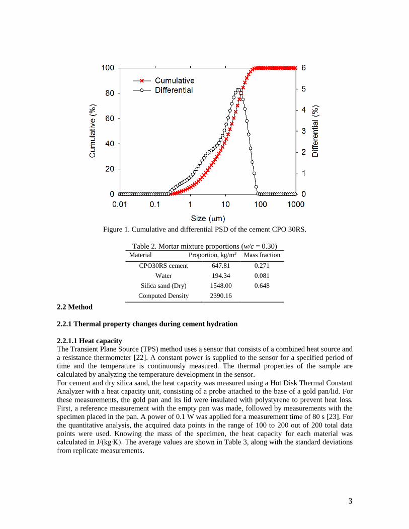
Figure 2 shows the values of thermal conductivity and specific heat obtained. A small variation of

the thermal properties with hydration time is observed. The experimental values (red points) of

specific heat were obtained as well as the thermal conductivity (blue triangles). Because the TPS

method provided the value of thermal diffusivity, based on this data, the value of the volumetric

specific heat was transformed into specific heat in units of J/(kg∙K). The densities of the material

were calculated from the actual dimensions and masses of the specimens.

5

Figure 2. Thermal conductivity and specific heat capacity of mortar with w/c = 0.30. The error bars

represent one standard deviation.

The thermal conductivity of the mortar was also calculated using the bounds of Hashin-

Shtrikman [23], shown in Figure 2 as the solid blue line, as the average of the lower (kl) and upper

(ku) bounds for thermal conductivity of a two-phase material. Equations (2) and (3) were used to

calculate the thermal conductivity as a function of the volume fraction of the hydrated cement paste

(x1) and the silica sand (x2). The obtained value was 2.8 W/(m∙K) for the mortar with a w/c ratio of

0.30. The bounds are given by:

1

1

12

21

3

1

k

x

kk

xkkl

(2)

2

2

21

12

3

1

k

x

kk

xkkh

(3)

where k1 was taken as 1 W/(m∙K) for the cement paste [23] and k2 was calculated as 5 W/(m∙K) for

the silica sand, according to the procedure described next. The value of 5 is on the lower end of the

range of 5 W/(m∙K) to 8 W/(m∙K) found in the literature for siliceous aggregates [23].

Based on the volumetric proportions of slurries prepared with only water and silica sand, the

thermal conductivity of the mix was measured using the aforementioned TPS method. Knowing the

thermal conductivity of water, equations (2) and (3) were then used to estimate the thermal

conductivity of silica sand.

2.2.1.3 Isothermal calorimetry

Using the mortar mixture proportions shown in Table 2, the heat release and heat flow during

cement hydration were measured using a TAM air isothermal calorimeter 1 [24]. A sample of

1 Certain commercial products are identified in this paper to specify the materials used and procedures employed. In no

case does such identification imply endorsement or recommendation by the National Institute of Standards and

Technology, nor does it indicate that the products are necessarily the best available for the purpose.

6

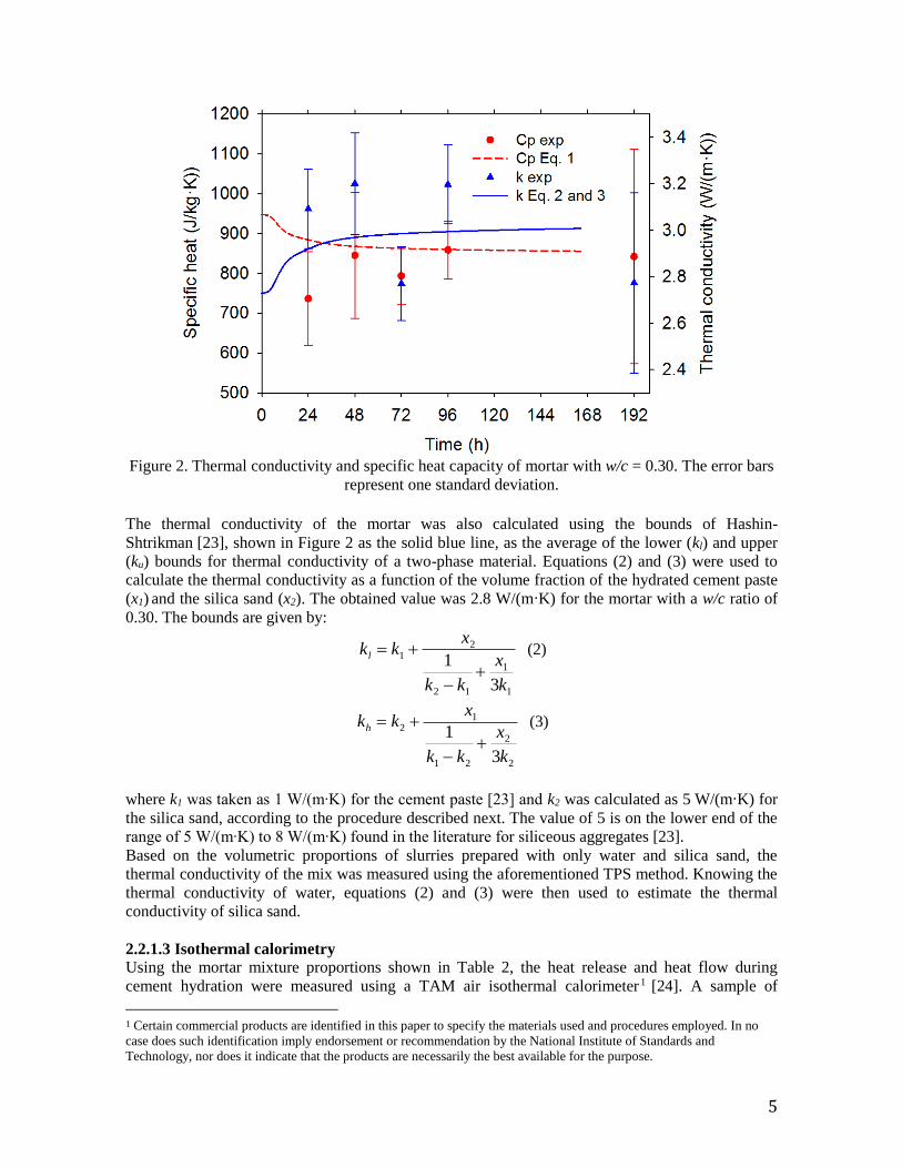
about 4 g to 8 g of each prepared mixture was placed into a 20 mL glass ampoule and sealed. The

measurements were made according to the user’s manual procedure, during 7 d to 9 d at 23 °C

and 38 ºC. The samples were cured under sealed conditions in the calorimeter.

Figure 3. Heat flow and heat release curves of mortar w/c = 0.30.

Based on the information shown in Figure 3, the parameters of the maturity model (Table 4) were

obtained by fitting the curve of cumulative heat release at 23 ºC to the maturity equation

(Equation 4), in order to obtain the parameters αu, β, and τ. The activation energy (J/mol) was

obtained from Equation (5), where the concept of equivalent time (equivalent age) was used to

compare the two data sets at 23 ºC and 38 ºC [25] The isothermal calorimetry tests were performed

on cement pastes at 23 °C, 38 °C, and 60 ºC. For the mortars, they were performed at 23 °C

and 38 ºC (Table 4), providing similar values compared to the cement pastes at the same

temperatures. Therefore, the value at 60 ºC obtained for the cement paste was also taken for the

mortar.

𝑑𝛼

𝑑𝑡= 𝑒𝑥𝑝 [

𝐸

𝑅(

1

𝑇𝑟−

1

𝑇)]

𝛼𝑢𝛽

𝑡𝑒(

𝜏

𝑡𝑒)

𝛽𝑒𝑥𝑝 [− (

𝜏

𝑡𝑒)

𝛽] , 𝑡 = 0 𝑡ℎ𝑒𝑛 𝛼 = 0 (4)

where α (te) is the degree of hydration at equivalent age te, τ is the hydration time (h), β is the

hydration shape parameter, which represents the slope of the linear portion of the hydration-time

relationship (larger values of β indicate a faster hydration rate), αu is the final degree of

hydration [2]. Values of these parameters for the mortar with w/c=0.30 are given in Table 4.

𝑑𝑡𝑒

𝑑𝑡= 𝑒𝑥𝑝 [

𝐸

𝑅(

1

𝑇𝑟−

1

𝑇)] , 𝑡 = 0 𝑡ℎ𝑒𝑛 𝑡𝑒 = 0 (5)

7

where te is the equivalent time or equivalent age at the reference curing temperature, dt is the

differential time (interval) (h), T is the average concrete temperature during the interval dt (K), Tr is

the constant reference temperature (taken to be 296.15 K in this study), E is the activation

energy (J/mol) and R is the universal gas constant (8.314 J/(mol∙K)). According to Jonasson et

al. (1995) [25], there is an almost linear relationship between the temperature and the activation

energy in the range of 23 ºC and higher. In our model, this relationship was considered by

interpolating the values given in Table 4.

Table 4 Maturity parameters and activation energy for the mortar obtained by fitting the isothermal

calorimetry data to Equation 4 (Correlation coefficient =0.998)

Maturity parameters Value Standard

error

αu 0.50 0.001

τ 10.09 0.132

β 0.98 0.016

Activation energy E 23 32800 (J/mol)

Activation energy E 60 25800(J/mol)

2.2.2 Semi-adiabatic calorimetry experiments (Type A specimens)

A semi-adiabatic calorimetry experiment was undertaken during 7 d to measure the temperature

evolution during hydration of the mortar. About 300 g of mortar was used to cast a Type A cylinder

in a low-density polyethylene (LDPE) container ( 46 mm x 99 mm). The calorimeter has a semi-

adiabatic configuration and contains a micro-silica insulation (k= 0.036 W/(m∙K) and

thickness=0.065 m) wall and a single thermocouple inserted approximately midway into the

specimen to record the temperature. The maximum heat loss was 8 J/h/K, which is less than

the 100 J/h/K required by RILEM [26] for a calorimeter to be considered as semi-adiabatic.

2.2.3 Steam curing experiments

2.2.3.1 Type B specimens under steam curing

Type B cylindrical mortar specimens ( 100 mm x 200 mm) were cast in polystyrene insulated

polyvinyl chloride (PVC) molds. The PVC prevents the mass transport in the radial direction. Only

one face of the specimens was not insulated, so that heat and mass transport are unidirectional

through this face. Before pouring the mortar into the molds, type K thermocouples with a range

of -130 °C to 90 °C and an accuracy of ± 0.28 °C were placed to monitor the temperature changes

during curing/hydration at seven evenly spaced locations along the specimens. The initial

temperature of the mortar was 24 °C. The experimental setup within the environmental chamber is

shown in Figure 4. The temperature and relative humidity inside the chamber were recorded with a

thermo-hygrometer having a range of 0 % to 100 % and an accuracy of ± 2.5 %.

8

a) b)

Figure 4. a) Experimental setup inside the environmental chamber, and b) Polystyrene insulated

PVC mold for Type B specimens, showing only three of the seven holes for the thermocouples.

Once the specimens were cast, they were kept inside the environmental chamber at approximately

100 % relative humidity and 24 ºC for a period of 3 h. Temperature readings at seven locations were

taken every minute throughout the entire curing process of 18 h, starting immediately after casting.

This provided the spatial temperature distribution inside the specimens. The locations of

thermocouples were labeled from 1 to 7 (1 being the thermocouple on the concrete surface and 7 the

thermocouple at the insulated base of the cylinder). Then, the specimens were subjected to the

steam-curing schedule shown in Figure 5, which is based on the ACI 517-2R-80 Standard for an

accelerated curing with water vapor at atmospheric pressure [27]. Addition of a steam generator

was necessary in order to ensure the required temperature and relative humidity within the

environmental chamber.

Figure 5. Steam curing schedule.

9

After the curing process, the specimens were cut into seven pieces, each one corresponding to the

region where the thermocouples were placed, with the aim of measuring the moisture content by

gravimetric measurements and the degree of hydration by loss on ignition.

2.2.3.2 NMR/MRI measurements during steam curing

Type C specimens ( 40 mm x 50 mm) were cast with the same mortar in polystyrene insulated

glass containers (Figure 6a). These specimens were subjected to the same steam curing as

specimens Type B, and were removed from the environmental chamber every 2 h during 15 min for

the NMR measurements. During testing, they were just covered with a thick cloth to reduce the heat

loss (Figure 6b). The temperature at the sample holder was maintained at 35 ºC. The CPMG [28]

and the Single Point Imaging (SPI) techniques [29] were used in an Oxford Instruments Maran

DRX HF 12/50 spectrometer. The CPMG technique allowed determination of the NMR signal

amplitude and the transverse relaxation time T2, associated with the evaporable water and the pore

size, respectively [30]. The SPI technique provided the water content distribution and the T2*

relaxation time by undertaking T2* mapping [31] with 10 encoding times. This bulk and spatially

resolved information was required to compare with the results obtained from the numerical

simulation.

a) b)

Figure 6. a) Type C mortar specimens for nondestructive NMR/MRI measurements. b) Type C

mortar specimens covered with a cloth in the sample holder.

3 Mathematical Modeling approach

3.1 Geometries

Three different geometries used in the experiments were modeled in COMSOL Multiphysics®

version 4.4, in a 2-D axisymmetric geometry with the domains framed by cylindrical coordinates.

The geometries represent the semi-adiabatic experiments with Type A specimens, the steam curing

experiments with Type B specimens, and the NMR/MRI water profile measurements with Type C

specimens. The dimensions of the geometries are given in millimeters.

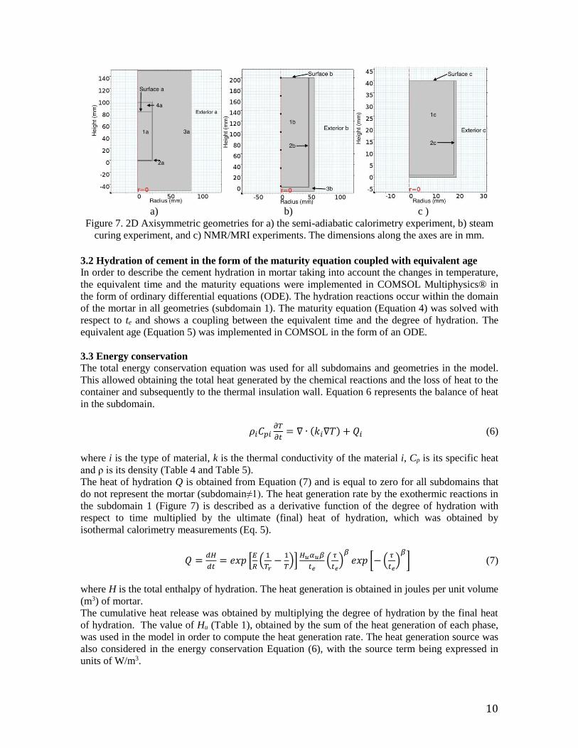
Figure 7a represents the geometry of the semi-adiabatic calorimetry experiment that consists of four

subdomains, which represent the material i: 1a) the cylinder of mortar; 2a) the container; 3a) the

insulation wall, and 4a) the air between the top surface of the mortar and the container lid. Figure 7b

represents the geometry used in the steam curing experiment that is composed of three subdomains:

1b) the mortar cylinder, 2b) the PVC container, and 3b) polystyrene insulation. Figure 7c represents

the geometry of the MRI specimens that consists of two subdomains: 1c) the mortar cylinder and

2c) the glass container.

10

a) b) c )

Figure 7. 2D Axisymmetric geometries for a) the semi-adiabatic calorimetry experiment, b) steam

curing experiment, and c) NMR/MRI experiments. The dimensions along the axes are in mm.

3.2 Hydration of cement in the form of the maturity equation coupled with equivalent age In order to describe the cement hydration in mortar taking into account the changes in temperature,

the equivalent time and the maturity equations were implemented in COMSOL Multiphysics® in

the form of ordinary differential equations (ODE). The hydration reactions occur within the domain

of the mortar in all geometries (subdomain 1). The maturity equation (Equation 4) was solved with

respect to te and shows a coupling between the equivalent time and the degree of hydration. The

equivalent age (Equation 5) was implemented in COMSOL in the form of an ODE.

3.3 Energy conservation The total energy conservation equation was used for all subdomains and geometries in the model.

This allowed obtaining the total heat generated by the chemical reactions and the loss of heat to the

container and subsequently to the thermal insulation wall. Equation 6 represents the balance of heat

in the subdomain.

𝜌𝑖𝐶𝑝𝑖𝜕𝑇

𝜕𝑡= ∇ ∙ (𝑘𝑖∇𝑇) + 𝑄𝑖

(6)

where i is the type of material, k is the thermal conductivity of the material i, Cp is its specific heat

and ρ is its density (Table 4 and Table 5).

The heat of hydration Q is obtained from Equation (7) and is equal to zero for all subdomains that

do not represent the mortar (subdomain≠1). The heat generation rate by the exothermic reactions in

the subdomain 1 (Figure 7) is described as a derivative function of the degree of hydration with

respect to time multiplied by the ultimate (final) heat of hydration, which was obtained by

isothermal calorimetry measurements (Eq. 5).

𝑄 =𝑑𝐻

𝑑𝑡= 𝑒𝑥𝑝 [

𝐸

𝑅(

1

𝑇𝑟−

1

𝑇)]

𝐻𝑢𝛼𝑢𝛽

𝑡𝑒(

𝜏

𝑡𝑒)

𝛽𝑒𝑥𝑝 [− (

𝜏

𝑡𝑒)

𝛽] (7)

where H is the total enthalpy of hydration. The heat generation is obtained in joules per unit volume

(m3) of mortar.

The cumulative heat release was obtained by multiplying the degree of hydration by the final heat

of hydration. The value of Hu (Table 1), obtained by the sum of the heat generation of each phase,

was used in the model in order to compute the heat generation rate. The heat generation source was

also considered in the energy conservation Equation (6), with the source term being expressed in

units of W/m3.

11

Table 5. Properties of materials i used in the experiments (from manufacturers)

Material Subdomain

number

Density

(kg/m3)

Heat capacity

[J/(kg∙K)]

Thermal

conductivity

[W/(m∙K)]

LPDE container 2a 920 1400 0.36

Micro-silica insulation 3a 230 800 0.037

Polyvinyl chloride 2b 1390 900 0.17

Polystyrene 3b 50 130 0.04

Glass 2c 2203 703 1.38

3.4 Moisture conservation The moisture conservation balance (Equation 8) was applied to the subdomain 1 of mortar in all of

the different geometries. This balance includes the transport of vapor (h) and liquid water, which is

the moisture content in the specimen. The physically bound water was not considered.

𝜌𝑠𝜕𝑤

𝜕𝑡=

𝜕

𝜕𝑥[𝜌𝑠𝐷𝑙

𝜕𝑤

𝜕𝑥+ 𝜌𝑠𝐷𝑣

𝜕ℎ

𝜕𝑥] + 𝑆 (8)

where ρs is the density of the solid, w is the moisture content (kg of water/kg of dry solid), h is the

relative humidity, and S is the sink of water due to hydration reactions. The diffusion coefficients of

liquid water Dl (Equation 9) and water vapor ρsDv (Equation 10) were taken from [33], previously

determined by Krus (1995), with values for a =0.0155 g/(m∙d), b= 0.0055, and c=144, as

determined for the mortars in the current study:

𝜌𝑠𝐷𝑣 = 𝑎

(9)

𝐷𝑙 = 𝑏𝑒𝑥𝑝(𝑐𝑤)

(10)

This coefficient depends on the moisture content. Therefore, it has a relationship with the degree of

hydration in the sink term (Equation 8). Another term obtained from the calculated degree of

hydration is the evaporable water sink S, which is the water consumed by the hydration reactions. S

will be considered in the equation of total moisture conservation (Equation 11).

𝑆 = −𝜌𝑠𝑀𝑓𝑐𝑒𝑚𝑤𝑛

𝑑𝛼

𝑑𝑡 (11)

where ρs is the solid density and wn is the non-evaporable water necessary for hydration, obtained as

the sum of the water necessary for the hydration of each phase in Table 1, and Mcemf is the mass

fraction of cement. The sink of water in the material is computed in units of kg/(m2∙s).

3.5 Boundary and initial conditions One of the assumptions of the model is that there exists a perfect contact between the materials.

Therefore, in the heat conservation equation, the applied interior boundary condition in all

geometries is a continuous boundary between air-mortar, mortar-container, and container-insulation

(Equation 12).

(12)

The mass conservation equation is applied to the domain of mortar, which has one boundary in

contact with the surrounding environment. Therefore, the boundary conditions in this domain are

12

zero flux conditions, except for the open surface (Table 6). The exterior boundaries in geometries b

and c have a boundary condition as described by the Equation 13.

(13)

Table 6. Boundary conditions Boundaries Geometry a Geometry b Geometry c

Heat Conservation Equation

Surface

(open)

(14)

(15)

Exterior (16)

Mass conservation Equation

Surface

(open) (17)

At the open surface of Type B and C specimens, a convective boundary condition was applied as

expressed by Equation 15, where hc is the convective heat transfer coefficient, vap is the heat of

vaporization, hm is the mass transfer coefficient at the surface, Pvext is the vapor pressure in the

surroundings [32], and Pv is the vapor pressure inside the material. For type A specimens, hc takes a

value of 15 W/(m2 ∙K) [11] for an enclosed environment. In the case of steam curing conditions

(Type B and C specimens), hc was calculated as 35.15 W/(m2 ∙K) using a trial and error method

(inverse method), adjusting the profiles of experimental temperature to match the simulated ones,

until reaching the lowest mean quadratic error.

For comparison, Smilauer and Krejci [11] propose a value of 31 W/(m2 ∙K) for a concrete surface

surrounded by water. Under steam curing condition, the hc value increases as the temperature and

the relative humidity inside the chamber increase. In the curing chamber there is not forced

convection, but only natural convection. In order to compute the heat transfer coefficient, both the

Grashof and Prandtl numbers are used, whose product gives the Raleigh number. The Raleigh

number takes into account the buoyancy effect. The heat transfer coefficient has been computed by

considering the experimental conditions present in the chamber, obtaining an average value of

35 W/(m2 ∙K).

The boundary condition (equation 17) for the mass conservation equation considers a convective

mass transfer coefficient of 6x10-3 g/(m2 ∙h ∙Pa). This value was calculated using a trial and error

method by comparing the average experimental kinetics with the simulated ones, until reaching the

lowest mean quadratic error. Villmman et al. [32] proposed a value of hm = 5x10-3 g/m2∙h∙Pa for

mortar with w/c=0.40 exposed to 23 ºC and 35 % relative humidity. The initial conditions were a

moisture content of 0.0885 kg water/kg dry solid and a temperature of 23 ºC for the semi-adiabatic

experiments, and 24 ºC for the steam curing conditions (Figure 5).

3.6 Numerical Solution.

A coupled model is employed for the simulation. Figure 8 shows the components of the

computational model and the couplings. The couplings between the energy conservation equations

and mass conservation equations are ensured by the boundary conditions. The equivalent time is an

input for the maturity equation, which computes the degree of hydration. The degree of hydration is

13

linked to the mass conservation equation by the sink term (S), which indicates the loss of moisture

due to chemical reaction. The degree of hydration is also connected to the energy conservation

equation by the source term (Q), which takes into account the exothermic nature of the reaction.

The constitutive equations are shown in Figure 8.

Figure 8. Components of the computational model and the couplings

Using a relative tolerance of 0.01, and a time step of 6 min, the set of equations was solved. The

triangular elements solved and the degrees of freedom in each geometry were as follows: Geometry

a Elements=1913 DOFs=10016, Geometry b Elements=1720 DOFs=19569, and Geometry c

Elements= 551 DOFs=8686.

4 Results and discussion

4.1 Semi-adiabatic experiment simulation

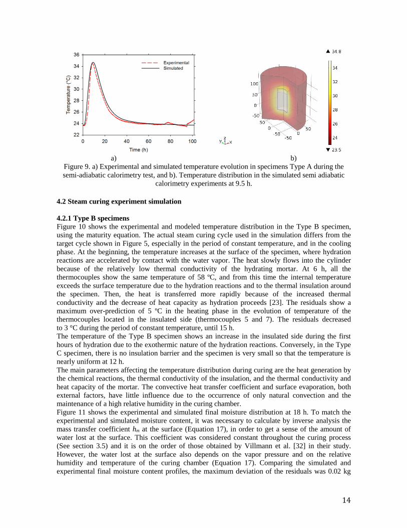
Figure 9 shows the comparison of temperature evolution between that measured for the Type A

cylinders in the semi-adiabatic calorimetry experiments (dotted line) and the result of the simulation

using the presented model (solid line). A good agreement is observed between the experimental and

the simulated data. The temperature first increases due to the heat generated by cement hydration.

The temperature distribution is homogeneous due to the low thermal conductivity of the micro-

silica insulation and to the mortar’s thermal conductivity that is dominated by the silica sand that

represents 64 % by mass of the specimen. The simulated maximum temperature of 34.7 ºC in this

specimen was reached at 9.5 h (Figure 9 b).

The temperature evolution shows the heating and cooling phases. Residuals were obtained from the

difference between the simulated and experimental data, obtaining a maximum difference of 2.5 °C,

in the heating phase. The difference was positive throughout the hydration process, which means an

over-prediction of temperature by the model. The residuals dropped below 1 ºC in the cooling

phase. It needs to be taken into account that there is a continuous boundary condition (Equation 14)

on the surface of the specimen and that there is air trapped between the lid and mortar; therefore the

model does not consider water evaporation (and its accompanying evaporative cooling) and this

may contribute to the temperature over-predictions. In support of this, liquid water has been

sometimes observed at the top surface of similar semi-adiabatic calorimetry specimens when they

were removed from their surrounding insulation after 3 d. In the semi-adiabatic calorimetry test, the

value assigned to the thermal conductivity of the insulation was critical in obtaining reasonable

agreement between the experiments and the simulation. The employed value from Table 5 was

obtained from direct measurement on the in service material using the TPS method and was

significantly higher than the value of about 0.02 W/(m∙K) supplied by the manufacturer for new

material.

14

a) b)

Figure 9. a) Experimental and simulated temperature evolution in specimens Type A during the

semi-adiabatic calorimetry test, and b). Temperature distribution in the simulated semi adiabatic

calorimetry experiments at 9.5 h.

4.2 Steam curing experiment simulation

4.2.1 Type B specimens

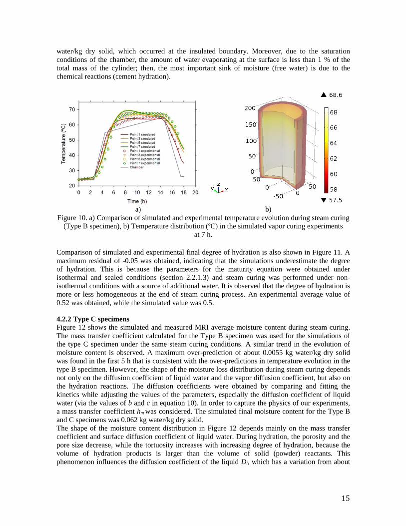
Figure 10 shows the experimental and modeled temperature distribution in the Type B specimen,

using the maturity equation. The actual steam curing cycle used in the simulation differs from the

target cycle shown in Figure 5, especially in the period of constant temperature, and in the cooling

phase. At the beginning, the temperature increases at the surface of the specimen, where hydration

reactions are accelerated by contact with the water vapor. The heat slowly flows into the cylinder

because of the relatively low thermal conductivity of the hydrating mortar. At 6 h, all the

thermocouples show the same temperature of 58 ºC, and from this time the internal temperature

exceeds the surface temperature due to the hydration reactions and to the thermal insulation around

the specimen. Then, the heat is transferred more rapidly because of the increased thermal

conductivity and the decrease of heat capacity as hydration proceeds [23]. The residuals show a

maximum over-prediction of 5 ºC in the heating phase in the evolution of temperature of the

thermocouples located in the insulated side (thermocouples 5 and 7). The residuals decreased

to 3 °C during the period of constant temperature, until 15 h.

The temperature of the Type B specimen shows an increase in the insulated side during the first

hours of hydration due to the exothermic nature of the hydration reactions. Conversely, in the Type

C specimen, there is no insulation barrier and the specimen is very small so that the temperature is

nearly uniform at 12 h. The main parameters affecting the temperature distribution during curing are the heat generation by

the chemical reactions, the thermal conductivity of the insulation, and the thermal conductivity and

heat capacity of the mortar. The convective heat transfer coefficient and surface evaporation, both

external factors, have little influence due to the occurrence of only natural convection and the

maintenance of a high relative humidity in the curing chamber.

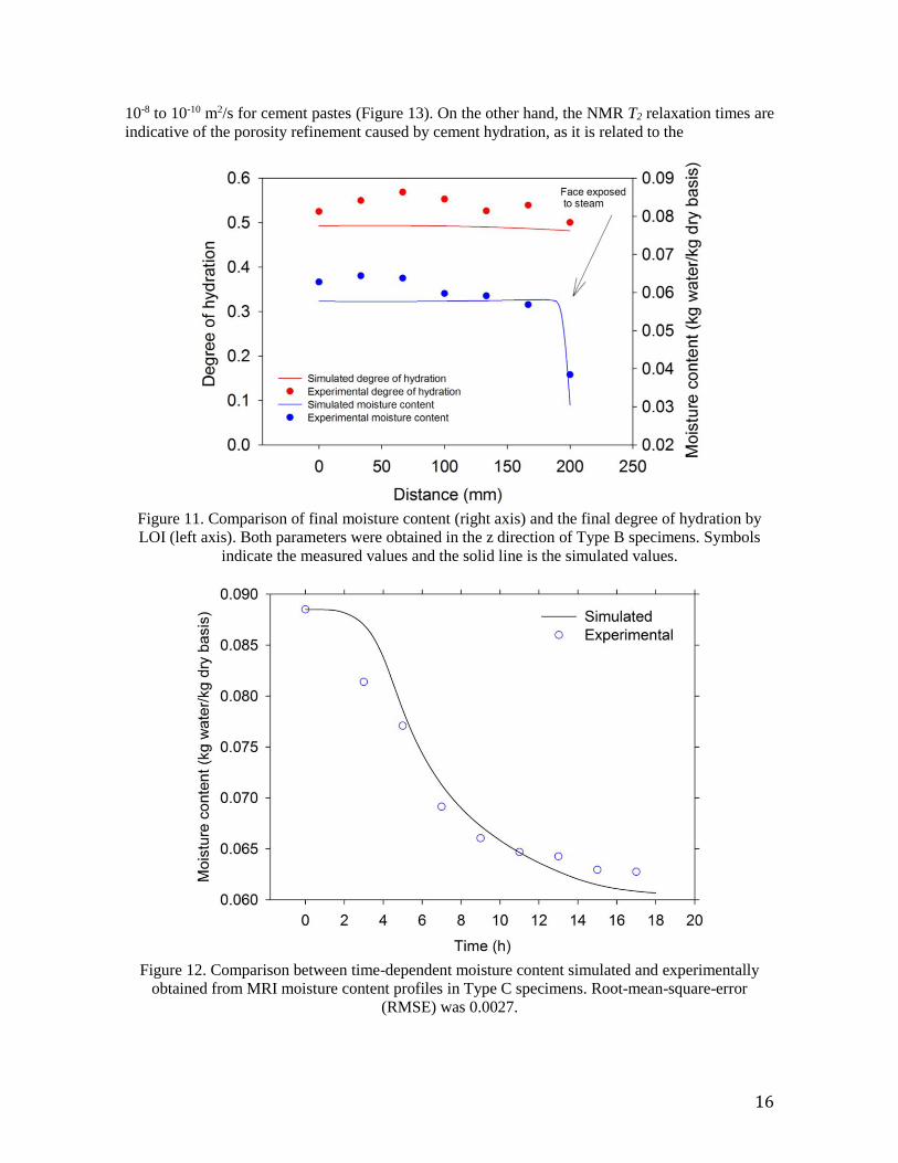
Figure 11 shows the experimental and simulated final moisture distribution at 18 h. To match the

experimental and simulated moisture content, it was necessary to calculate by inverse analysis the

mass transfer coefficient hm at the surface (Equation 17), in order to get a sense of the amount of

water lost at the surface. This coefficient was considered constant throughout the curing process

(See section 3.5) and it is on the order of those obtained by Villmann et al. [32] in their study.

However, the water lost at the surface also depends on the vapor pressure and on the relative

humidity and temperature of the curing chamber (Equation 17). Comparing the simulated and

experimental final moisture content profiles, the maximum deviation of the residuals was 0.02 kg

15

water/kg dry solid, which occurred at the insulated boundary. Moreover, due to the saturation

conditions of the chamber, the amount of water evaporating at the surface is less than 1 % of the

total mass of the cylinder; then, the most important sink of moisture (free water) is due to the

chemical reactions (cement hydration).

a) b)

Figure 10. a) Comparison of simulated and experimental temperature evolution during steam curing

(Type B specimen), b) Temperature distribution (ºC) in the simulated vapor curing experiments

at 7 h.

Comparison of simulated and experimental final degree of hydration is also shown in Figure 11. A

maximum residual of -0.05 was obtained, indicating that the simulations underestimate the degree

of hydration. This is because the parameters for the maturity equation were obtained under

isothermal and sealed conditions (section 2.2.1.3) and steam curing was performed under non-

isothermal conditions with a source of additional water. It is observed that the degree of hydration is

more or less homogeneous at the end of steam curing process. An experimental average value of

0.52 was obtained, while the simulated value was 0.5.

4.2.2 Type C specimens

Figure 12 shows the simulated and measured MRI average moisture content during steam curing.

The mass transfer coefficient calculated for the Type B specimen was used for the simulations of

the type C specimen under the same steam curing conditions. A similar trend in the evolution of

moisture content is observed. A maximum over-prediction of about 0.0055 kg water/kg dry solid

was found in the first 5 h that is consistent with the over-predictions in temperature evolution in the

type B specimen. However, the shape of the moisture loss distribution during steam curing depends

not only on the diffusion coefficient of liquid water and the vapor diffusion coefficient, but also on

the hydration reactions. The diffusion coefficients were obtained by comparing and fitting the

kinetics while adjusting the values of the parameters, especially the diffusion coefficient of liquid

water (via the values of b and c in equation 10). In order to capture the physics of our experiments,

a mass transfer coefficient hm was considered. The simulated final moisture content for the Type B

and C specimens was 0.062 kg water/kg dry solid.

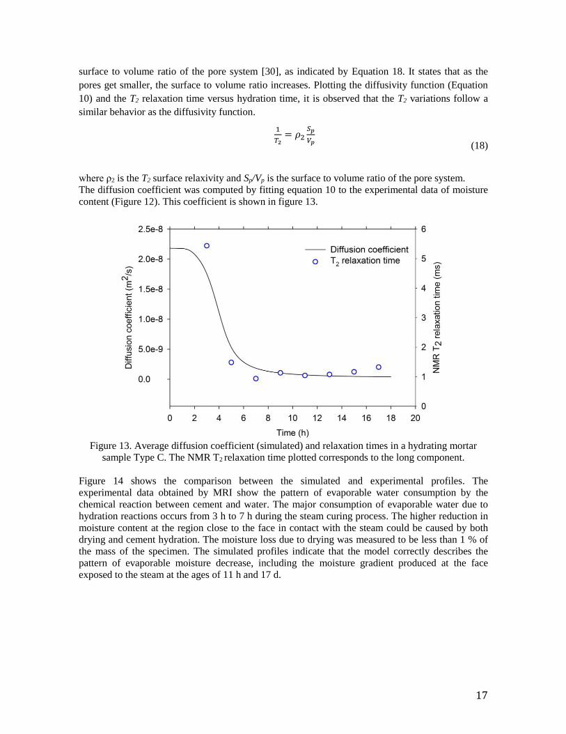
The shape of the moisture content distribution in Figure 12 depends mainly on the mass transfer

coefficient and surface diffusion coefficient of liquid water. During hydration, the porosity and the

pore size decrease, while the tortuosity increases with increasing degree of hydration, because the

volume of hydration products is larger than the volume of solid (powder) reactants. This

phenomenon influences the diffusion coefficient of the liquid Dl, which has a variation from about

16

10-8 to 10-10 m2/s for cement pastes (Figure 13). On the other hand, the NMR T2 relaxation times are

indicative of the porosity refinement caused by cement hydration, as it is related to the

Figure 11. Comparison of final moisture content (right axis) and the final degree of hydration by

LOI (left axis). Both parameters were obtained in the z direction of Type B specimens. Symbols

indicate the measured values and the solid line is the simulated values.

Figure 12. Comparison between time-dependent moisture content simulated and experimentally

obtained from MRI moisture content profiles in Type C specimens. Root-mean-square-error

(RMSE) was 0.0027.

17

surface to volume ratio of the pore system [30], as indicated by Equation 18. It states that as the

pores get smaller, the surface to volume ratio increases. Plotting the diffusivity function (Equation

10) and the T2 relaxation time versus hydration time, it is observed that the T2 variations follow a

similar behavior as the diffusivity function.

1

𝑇2= 𝜌2

𝑆𝑝

𝑉𝑝

(18)

where ρ2 is the T2 surface relaxivity and Sp/Vp is the surface to volume ratio of the pore system.

The diffusion coefficient was computed by fitting equation 10 to the experimental data of moisture

content (Figure 12). This coefficient is shown in figure 13.

Figure 13. Average diffusion coefficient (simulated) and relaxation times in a hydrating mortar

sample Type C. The NMR T2 relaxation time plotted corresponds to the long component.

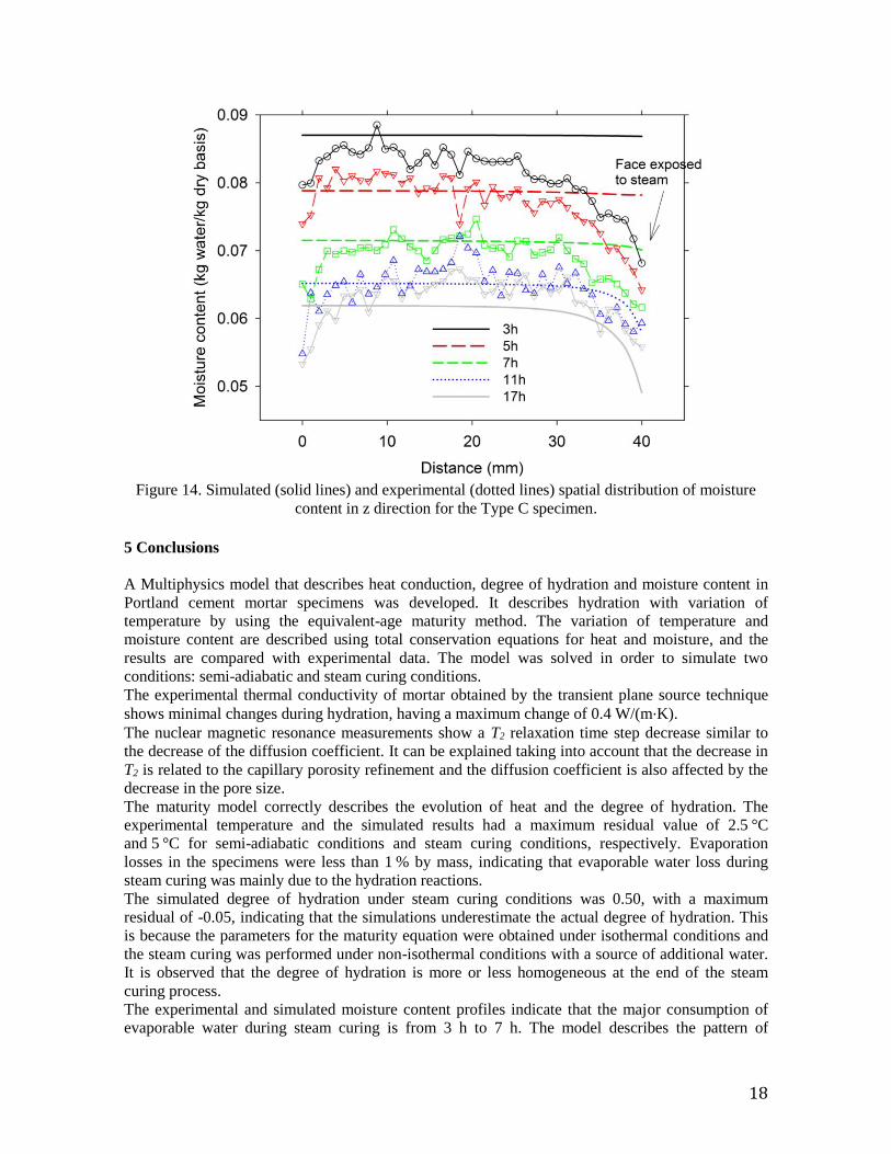
Figure 14 shows the comparison between the simulated and experimental profiles. The

experimental data obtained by MRI show the pattern of evaporable water consumption by the

chemical reaction between cement and water. The major consumption of evaporable water due to

hydration reactions occurs from 3 h to 7 h during the steam curing process. The higher reduction in

moisture content at the region close to the face in contact with the steam could be caused by both

drying and cement hydration. The moisture loss due to drying was measured to be less than 1 % of

the mass of the specimen. The simulated profiles indicate that the model correctly describes the

pattern of evaporable moisture decrease, including the moisture gradient produced at the face

exposed to the steam at the ages of 11 h and 17 d.

18

Figure 14. Simulated (solid lines) and experimental (dotted lines) spatial distribution of moisture

content in z direction for the Type C specimen.

5 Conclusions

A Multiphysics model that describes heat conduction, degree of hydration and moisture content in

Portland cement mortar specimens was developed. It describes hydration with variation of

temperature by using the equivalent-age maturity method. The variation of temperature and

moisture content are described using total conservation equations for heat and moisture, and the

results are compared with experimental data. The model was solved in order to simulate two

conditions: semi-adiabatic and steam curing conditions.

The experimental thermal conductivity of mortar obtained by the transient plane source technique

shows minimal changes during hydration, having a maximum change of 0.4 W/(m∙K).

The nuclear magnetic resonance measurements show a T2 relaxation time step decrease similar to

the decrease of the diffusion coefficient. It can be explained taking into account that the decrease in

T2 is related to the capillary porosity refinement and the diffusion coefficient is also affected by the

decrease in the pore size.

The maturity model correctly describes the evolution of heat and the degree of hydration. The

experimental temperature and the simulated results had a maximum residual value of 2.5 °C

and 5 °C for semi-adiabatic conditions and steam curing conditions, respectively. Evaporation

losses in the specimens were less than 1 % by mass, indicating that evaporable water loss during

steam curing was mainly due to the hydration reactions.

The simulated degree of hydration under steam curing conditions was 0.50, with a maximum

residual of -0.05, indicating that the simulations underestimate the actual degree of hydration. This

is because the parameters for the maturity equation were obtained under isothermal conditions and

the steam curing was performed under non-isothermal conditions with a source of additional water.

It is observed that the degree of hydration is more or less homogeneous at the end of the steam

curing process.

The experimental and simulated moisture content profiles indicate that the major consumption of

evaporable water during steam curing is from 3 h to 7 h. The model describes the pattern of

19

evaporable water consumption by chemical reaction and evaporation at the surface of the specimen,

compared with the experimental profiles.

Acknowledgements

E. Hernández-Bautista acknowledges NIST and the staff of their Materials and Structural Systems

Division, Conacyt for the PhD scholarship and the Instituto Politécnico Nacional for the PIFI

scholarship. P. Cano and S. Sandoval acknowledge SIP from IPN for funding the projects ID codes

20140613 and 20144660, respectively.

Nomenclature

a Parameter for vapor diffusion coefficient kg/(m∙s)

b Parameter for the liquid diffusion coefficient

c Parameter for the liquid diffusion coefficient

CpCemBM Cement-based material specific heat capacity J/(kg∙K)

Cpi Specific heat capacity of the material i J/(kg∙K)

Dl Liquid moisture diffusion coefficient m2/s

Dv Vapor diffusion coefficient kg/(m∙s)

E Activation energy J/mol

H Total enthalpy of hydration J/kg

Hu Ultimate enthalpy of hydration J/kg

hc Convective heat transfer coefficient W/(m2 ∙K)

hm Mass transfer coefficient (s/m)

i type of Material

kl Hashin-Shtrikman lower bound for the thermal conductivity W/(m∙K)

kh Hashin-Shtrikman upper bound for the thermal conductivity W/(m∙K)

k1 Thermal conductivity of cement powder W/(m∙K)

k2 Thermal conductivity of silica sand W/(m∙K)

ki Thermal conductivity of material i W/(m∙K)

Mf water Water mass fraction

Mf Bondwater Bound water mass fraction

Mf cem Cement mass fraction

Mf silicasand Aggregate mass fraction

Normal vector

Pvext Vapor pressure in the surroundings Pa

Pv Vapor pressure inside the material Pa

Q Heat generation rate W/m3

R Ideal gas constant J/(mol∙K)

S Evaporable water sink kg/(m3∙s)

Sp Surface of the pore system m2

t Time s

Tr Reference temperature K

T Temperature K

te Equivalent time

T2 transverse relaxation time (s)

x1 Volume fraction of cement powder in the mix

x2 Volume fraction of silica sand in the mix

Vp Volume of the pore system m3

w Moisture content

20

Greek symbols

α Degree of hydration

αu Ultimate degree of hydration

β Maturity equation parameter

λvap Heat of vaporization J/kg

ρi Density of material i kg/m3

ρs Density of the solid cement-based material kg/m3

ρ2 Surface relaxivity m/s

τ Maturity equation parameter s

Ω Domain

References

[1] Kosmatka S. H., Kerkhoff B., and Panarese W. C., Design and Control Design and Control of

Concrete Mixtures, Fourteenth. Portland Cement Association 2003; p. 360.

[2] Xu Q., Ruiz J. M., Hu J., Wang K., and Rasmussen R. O.Modeling hydration properties and

temperature developments of early-age concrete pavement using calorimetry tests

Thermochim. Acta, 2011; 512(1–2): 76–85

[3] Soroka I. and Bentur H. J. A., Short-term steam-curing and concrete later-age strength

Materiaux et Constructions 1978;11(62): pp. 93–96,.

[4] Chini A. R., Effect of elevated curing temperatures on the strength and durability of concrete

Materials and Structures 2005; 38(281): 673–679

[5] Won I., Na Y., Kim J. T., and Kim S., Energy-efficient algorithms of the steam curing for the

in situ production of precast concrete members, Energy Build. 2013; 64: pp. 275–284

[6] Ramezanianpour A. A., Khazali M. H., and Vosoughi P., Effect of steam curing cycles on

strength and durability of SCC: A case study in precast concrete Construction and Building

Materials 2013; 49: pp. 807–813

[7] Kjellsen K., Heat curing and post-heat curing regimes of high- performance concrete: influence

on microstructure and C-S-H composition Cement and Concrete Research 1996; 26(2): pp.

295–307

[8] Ba M., Qian C., Guo X., and Han X. Effects of steam curing on strength and porous structure

of concrete with low water/binder ratio Construction and Building Materials 2011; 25(1): pp.

123–128

[9] Zhi-min, H E., Guang-cheng L., and You-jun X. I. E. Influence of subsequent curing on water

sorptivity and pore structure of steam-cured concrete J. Cent. South Univ. 2012; 12(19): pp.

1155–1162

[10] Ozkul M. H., Efficiency of accelerated curing in concrete Cement and Concrete Research

2001;31: pp. 1351–1357

21

[11] Smilauer V. and Krejci T., Multiscale model for temperature distribution in hydrating concrete

International Journal for Multiscale Computational Engineering 2009; 7(2)

[12] Davie C. T., Pearce C. J., and Bićanić N., Coupled Heat and Moisture Transport in Concrete at

Elevated Temperatures—Effects of Capillary Pressure and Adsorbed Water Numerical Heat

Transfer, Part A: Applications 2006; 49(8) : pp. 733–763

[13] Jeong J.-H. , Ligang W., and Zollinger D. G., A temperature and moisture module for

hydrating Portland cement concrete pavements in 7th International Conference on Concrete

Pavements, 2001; pp. 9–13.

[14] Sciumè G. and Schrefler B. A. A multi-scale numerical model for concrete at early age XVIII

GIMC Conference. Siracusa 2010

[15] Zhang B. and Yu X., Multiphysics for Early Stage Cement Hydration: Theoretical Framework

Advanced Materials Research. 2011; 216: 4247–4250

[16] Giovanni D., Luzio and Cusatis G. Hygro-Thermo-Chemical Modeling of High Performance

Concrete . I : Theory Introduction Cement & Concrete Composites 2009; 31(5): pp. 301–308.

[17] Lawrence A. M., Tia M., and Bergin M. Considerations for Handling of Mass Concrete :

Control of Internal Restraint ACI Materials Journal 2014;111: pp. 3–11

[18] ASTM. C188 Standard Test Method for Density of Hydraulic Cement ASTM International

2009

[19] ASTM Standard Practice for Mechanical Mixing of Hydraulic Cement Pastes and Mortars of

Plastic Consistency, ASTM International 2010: C305(06); pp. 6–8

[20] Bentz, D.P., Waller, V., and de Larrard, F. Prediction of adiabatic temperature rise in

conventional and high-performance concretes using a 3-D microstructural model. Cement and

Concrete Research 1998; 28 (2): pp. 285-297

[21] Hua C., Ehrlacher A., and Acker P. Analyses and model of the autogeous shrinkage of

hardening cement paste. II Modelling at scale of hydrating grains Cement and Concrete

Research 1997; 27(2): pp. 245–258,.

[22] Gustavsson S. E. Transient plane source technique for thermal conductivity and thermal

diffusivity measurements of solid materials Rev. Sci. Instrum, 1991; 62: pp. 797–804,

[23] Bentz D. P., Transient plane source measurements of the thermal properties of hydrating

cement pastes Materials and Structures 2007; 40: pp. 1073–1080

[24] Thermometric AB. HandbookTAM Air Calorimeter. New Castle 2011; p. 63.

[25] Schindler A. K. Temperature Control During Construction to Improve the Long Term

Performance of Portland Cement Concrete Pavements. Texas Department of Transportation,

2002

22

[26] RILEM. Adiabatic and semi-adiabatic calorimetry to determine the temperature increase in

concrete due to hydration heat of the cement. Materials and Structures 1997:30(8), 451–464

[27] American Concrete Institute. ACI 517-2R-80 Accelerated Curing of Concrete at Atmospheric

Pressure. ACI Journal 1980; 77: pp. 429–448

[28] Meiboom S. and Gill D. Modified spin–echo method for measuring nuclear relaxation times

Review of Scientific Instruments. 1958; 29: pp. 688–691

[29] Gravina S. and. Cory D. G. Sensitivity and resolution of constant-time imaging Journal of

Magnetic Resonance. 1994: Series B 1: pp. 53–61

[30] Halperin W. P. Microstructure Determination of Cement Pastes by NMR and Conventional

Techniques Advances in Cement-Based materials. 1993;1(2:) pp. 67–76

[31] Prado P. J., Balcom B. J., S. Beya D., Armstrong R. L., and Bremner T. W., Concrete/mortar

water phase transition studied by single-point MRI methods Magn. Reson. Imaging

1998:16(1): pp. 521–523

[32] Villmann B., Slowik V., Wittmann F. H., Vontobel P., and Hovind J. Time-dependent

Moisture Distribution in Drying Cement Mortars. Results of Neutron Radiography and Inverse

Analysis of Drying Tests Determination of Moisture Transport Parameters and Moisture

Profiles by Inverse Analysis. Restoration of Buildings and Monuments. 2014; 20(1): pp. 49–62

[33] Krus M. Feuchtetransport- und Speicherko effizienten poröser mineralischer Baustoffe.

Universität Stutt. 1995