accepted manuscript - los alamos national...
TRANSCRIPT

Accepted Manuscript
A comparative study of interface reconstruction methods for multi-material
ALE simulations
Milan Kucharik, Rao V. Garimella, Samuel P. Schofield, Mikhail J. Shashkov
PII: S0021-9991(09)00389-1
DOI: 10.1016/j.jcp.2009.07.009
Reference: YJCPH 2671
To appear in: Journal of Computational Physics
Received Date: 9 March 2009
Revised Date: 3 July 2009
Accepted Date: 13 July 2009
Please cite this article as: M. Kucharik, R.V. Garimella, S.P. Schofield, M.J. Shashkov, A comparative study of
interface reconstruction methods for multi-material ALE simulations, Journal of Computational Physics (2009),
doi: 10.1016/j.jcp.2009.07.009
This is a PDF file of an unedited manuscript that has been accepted for publication. As a service to our customers
we are providing this early version of the manuscript. The manuscript will undergo copyediting, typesetting, and
review of the resulting proof before it is published in its final form. Please note that during the production process
errors may be discovered which could affect the content, and all legal disclaimers that apply to the journal pertain.

ACCEPTED MANUSCRIPT 1 2 3 4 5 6 7 8 9 10 11 12 13 14 15 16 17 18 19 20 21 22 23 24 25 26 27 28 29 30 31 32 33 34 35 36 37 38 39 40 41 42 43 44 45 46 47 48 49 50 51 52 53 54 55 56 57 58 59 60 61 62 63 64 65
A comparative study of interface
reconstruction methods for multi-material
ALE simulations
Milan Kucharik
Applied Math and Plasma Physics (T-5), Los Alamos National Laboratory
Rao V. Garimella
Applied Math and Plasma Physics (T-5), Los Alamos National Laboratory
Samuel P. Schofield
Applied Math and Plasma Physics (T-5), Los Alamos National Laboratory
Mikhail J. Shashkov
Applied Math and Plasma Physics (T-5), Los Alamos National Laboratory
Abstract
In this paper we compare the performance of different methods for reconstructinginterfaces in multi-material compressible flow simulations. The methods comparedare a material-order-dependent Volume-of-Fluid (VOF) method, a material-order-independent VOF method based on power diagram partitioning of cells and theMoment-of-Fluid method (MOF). We demonstrate that the MOF method providesthe most accurate tracking of interfaces, followed by the VOF method with the rightmaterial ordering. The material-order-independent VOF method performs some-what worse than the above two while the solutions with VOF using the wrongmaterial order are considerably worse.
Key words:Interface Reconstruction, Moment-of-fluid method, compressible flow
Email addresses: [email protected], [email protected]
(Milan Kucharik), [email protected] (Rao V. Garimella), [email protected] (Samuel P.Schofield), [email protected] (Mikhail J. Shashkov).
Preprint submitted to Journal of Computational Physics 3 July 2009

ACCEPTED MANUSCRIPT 1 2 3 4 5 6 7 8 9 10 11 12 13 14 15 16 17 18 19 20 21 22 23 24 25 26 27 28 29 30 31 32 33 34 35 36 37 38 39 40 41 42 43 44 45 46 47 48 49 50 51 52 53 54 55 56 57 58 59 60 61 62 63 64 65
1 Introduction
Accurate simulation of multi-material and multi-phase flows requires effec-tive tracking and management of material interfaces. Due to their ability tostrictly conserve the mass of different materials, volume-of-fluid (VOF) meth-ods using interface reconstruction are widely used in such simulations [1–4].Originally developed by Hirt and Nichols [5], VOF methods do not explicitlytrack interfaces but rather track the volume of each material. The interfacebetween materials is first reconstructed in cells based on the material volumefractions. Then the volume fluxes of each material between cells are estimatedfrom the geometric reconstruction and finally, the fluxes are used to computenew volume fractions in each cell, in preparation for the next time step.
More recently, an interface tracking method has been devised based on track-ing both the volume (zeroth moment) and centroid (ratio of first and zerothmoment) of the materials in mesh cells. This new method, called the Moment-of-Fluid (MOF) method [6], reconstructs interfaces more accurately than VOFmethods and is able to resolve interfacial features on the order of the localmesh size whereas VOF methods do poorly in resolving features smaller than3-4 times the local mesh size.
In this paper, we present a comparative study of different VOF methods andthe MOF method for complex compressible flow simulations involving morethan two materials. It is organized as follows: in Section 2, we present a briefoverview of the common material order-dependent VOF methods. We describethe basic principle of each method and focus mainly on the Youngs’ VOFmethod, which is implemented in most multi-material codes. We describe theproblems with choosing the correct material ordering for such methods. In Sec-tion 3, we describe the order independent VOF method based on the powerdiagrams. In Section 4, the MOF material reconstruction method is described.The slope of the material interface is not determined from the volume fractionsof the neighboring cells, but from the material centroids of the particular cell.In Section 5, we briefly describe all steps of the ALE algorithm implementedin our research multi-material code. We focus mainly on the propagation ofthe material centroids needed for the MOF material reconstruction during theLagrangian and remapping steps of the algorithm. Coupling of the material re-construction methods with a multi-material ALE code is described. Section 6is the key part of the paper. It includes comparison of the described materialreconstruction methods in the context of particular multi-material hydrody-namic simulations including typical phenomena appearing in real problems –vortex, explosion, and a shock wave-material interaction. All numerical ex-amples include more than 2 materials to emphasize key properties of eachmethod. Finally, we conclude the paper and review the material reconstruc-tion methods in Section 7.
2

ACCEPTED MANUSCRIPT 1 2 3 4 5 6 7 8 9 10 11 12 13 14 15 16 17 18 19 20 21 22 23 24 25 26 27 28 29 30 31 32 33 34 35 36 37 38 39 40 41 42 43 44 45 46 47 48 49 50 51 52 53 54 55 56 57 58 59 60 61 62 63 64 65
2 VOF Methods with Nested Dissection (VOF-PLIC)
Early VOF methods used a straight line aligned with a coordinate axis topartition the cell according to the material volume fractions. This is oftenreferred to as the simple line interface calculation (SLIC) originally due toNoh and Woodward [7]. Youngs [8,9] extended the method to permit thematerial interface to have an arbitrary orientation within the cell (called PLICor Piecewise Linear Interface Calculation by Rider and Kothe [3]). In Youngs’method, the outward normal of the interface separating a material from therest of the cell is taken to be the negative gradient of the “volume fractionfunction”. The “volume fraction function” is treated as a smooth functionwhose cell-centered values are given by the cell-wise material volume fractions.The interface is then defined by locating a line with the prescribed normal thatcuts off the correct volume of material from the computational cell.
Gradient based methods are in general first order accurate although theymay exhibit near second order accuracy on regular Cartesian grids. However,there are extensions that make the reconstruction second-order accurate forgeneral grids. The LVIRA technique by Pilliod and Puckett [10] tries to find anextended straight line interface that cuts off the exact volume fraction in thecell of interest and minimizes the error in matching the volume fractions in thesurrounding cells. LVIRA uses a minimization procedure with a gradient-basednormal as the initial guess. An alternative is the interface smoothing procedurebased on Swartz’s quadratically convergent procedure [11] for finding a straightline that cuts off the right volume fractions from two arbitrary planar shapes 1 .Mosso et.al [14] and Garimella et.al. [15] have used this procedure in slightlydifferent ways to devise interface smoothing procedures. For a given mixed cell,Garimella et.al. compute a straight line cutting off the right volume fractionsfrom the cell and each of its mixed cell neighbors by the Swartz method. Thenormals of these different straight lines are then averaged to give a smoothedinterface normal for the cell.
VOF-PLIC techniques have been successfully used to accurately simulate two-phase (or two-material) flows and free-surface flows in two and three dimen-sions. However, their application to flows involving three or more materialsthat come closer than the mesh spacing and even form junctions has beenmostly ad hoc. Examples of such phenomena are flows of immiscible fluids(e.g. oil-water-gas), inertial confinement fusion, armor-antiarmor penetrationand powder metallurgical simulation of multiple materials.
The most common extensions of PLIC to cells with more than two materials
1 This is commonly known as the “ham-sandwich” or Steinhaus problem[12,13]
3

ACCEPTED MANUSCRIPT 1 2 3 4 5 6 7 8 9 10 11 12 13 14 15 16 17 18 19 20 21 22 23 24 25 26 27 28 29 30 31 32 33 34 35 36 37 38 39 40 41 42 43 44 45 46 47 48 49 50 51 52 53 54 55 56 57 58 59 60 61 62 63 64 65
A
C
A
C
B
A
C
B
A
(a) (b) (c) (d)
C C
A
C
B
A
C
B
A
(e) (f) (g) (h)
Fig. 1. Nested dissection interface reconstruction for three materials in the orderACB: (a) the first (A) material is removed leaving a smaller available polygon, (b)the second (C) material is removed from the available polygon, (c) the remainingavailable polygon is assigned to material B, (d) the resulting partitioning of thecomputational cell. (e)-(g) show the same procedure but the materials are processedin a different (CAB) order leading to a different reconstruction (h).
(multi-material cells) 2 , is to process materials one by one leading to a re-construction that is strongly dependent on the order in which the materialsare processed. Of the different ways to sequentially partition a cell, one ofthe most general and accurate ways is called the “nested dissection” method[6], where each material is separated from the others in a specified order. Inthe method, a pure polygon (or polyhedron) representing the first material ismarked out from the cell, leaving a mixed polygon for the remaining materi-als. Then, a polygon representing the second material is marked out from themixed polygon and the process continues until the last material is processed.This method is illustrated in Figure 1 and described in detail in [6,16,17].Clearly, such an order dependent method can easily place materials in wronglocations in the cells if the chosen order of processing is incorrect. Even if theorder of the materials is right, the computation of the interface normals inmulti-material cells is ambiguous. In computing the normal as the negativegradient of the volume fraction function of a material, it is unclear whetherone should use the volume fractions with respect to original cells or the partof the cells remaining after the earlier materials have been removed. It is also
2 In a strict sense, any cell with more than one material is a multi-material cell.However, we choose to distinguish two material cells from cells with more than twomaterials by calling the latter multi-material cells. The reason for this distinctionis that interface reconstruction for one material is (in the case of VOF methods)complementary to the second in a cell with two-materials while it is not for morethan two materials
4

ACCEPTED MANUSCRIPT 1 2 3 4 5 6 7 8 9 10 11 12 13 14 15 16 17 18 19 20 21 22 23 24 25 26 27 28 29 30 31 32 33 34 35 36 37 38 39 40 41 42 43 44 45 46 47 48 49 50 51 52 53 54 55 56 57 58 59 60 61 62 63 64 65
1
2 3
4 5
3
1 2
4 5
5
1 2
3 4
MOF Powerdiagram Youngs1 Youngs2 Youngs3
Fig. 2. Four material disk at time T = 0.5 translated from the initial position(0.2, 0.2) with 30 time steps at a velocity of (1, 1) on 32 × 32 mesh of the [0, 1]2
domain. Material reconstruction done by several methods – MOF, VOF with powerdiagrams, and Youngs’ VOF. The material orderings for Youngs’ are indicated inthe figure.
not clear where these function values should be centered – at the center of theoriginal cell or the center of the unprocessed part of the cell.
The most significant adverse effect of these incorrect reconstructions, however,is in material advection in flow simulations. An improper material orderingmay result in materials being advected prematurely (or belatedly) into neigh-boring cells. This can further lead to small pieces of the material gettingseparated and drifting away from the bulk of the material (sometimes knownas “flotsam and jetsam”). The effect of material ordering is illustrated clearlyin an example from [18] in which a four-material disk (with each material oc-cupying one quadrant of the disk) is advected diagonally for 30 time steps. Theresults in Figure 2 show dramatically different results with different materialorderings and a complete loss of the cross-shaped interface.
The most common and trivial way to deal with the material order depen-dency is to select the “correct” global ordering for a problem. However, thisis obviously problematic if the same materials must be processed differentlyin different parts of the mesh or if the material configurations change as theproblem advances in time. Also, some interface configurations may not be re-producible by any particular order, such as the four material example referredto above. While there has been some work on automatically deriving mate-rial order, most of these attempts assume a layered structure for the interface[14,19] and cannot handle multiple materials coming together at a point verywell.
3 VOF Methods with Power Diagram Reconstruction (VOF-PD)
Recently, Schofield et. al. [18] developed a new VOF-based reconstructionmethod that is completely material order independent. This method, calledthe Power Diagram method for Interface Reconstruction, does not sequen-tially carve off materials from a cell using straight lines. Rather it first lo-
5

ACCEPTED MANUSCRIPT 1 2 3 4 5 6 7 8 9 10 11 12 13 14 15 16 17 18 19 20 21 22 23 24 25 26 27 28 29 30 31 32 33 34 35 36 37 38 39 40 41 42 43 44 45 46 47 48 49 50 51 52 53 54 55 56 57 58 59 60 61 62 63 64 65
cates materials approximately in multi-material cells and then partitions thecell simultaneously into multiple material regions using a weighted Voronoidecomposition thereby avoiding the order dependence problem. We describethis procedure below referring to it as the VOF-PD method.
In the first step of the VOF-PD method, approximate locations or “centroids”of the materials in a cell are determined using the volume fractions of thematerials in the cell and its neighbors. This is accomplished by treating thevolume fractions of each material in the cell and its neighbors as pointwise val-ues of a pseudo-density function. The pointwise values of this pseudo-densityfunction are then used to obtain a linear reconstruction of the function alongwith application of a limiter restricting the minimum and maximum valuesto 0 and 1 respectively. Then the linear approximation of this pseudo-densityfunction is used to derive an approximate centroid for the material in the cell.While this method does not locate the material centroids very accurately inan absolute sense, it does locate the materials quite well relative to each other.
In the second step of the procedure, the approximate centroids of the materialsare used as generators for a weighted Voronoi or Power Diagram subdivision[20,21] of the cell. The weights of the different generators are chosen iterativelysuch that the volume fractions of the different Voronoi polygons truncated bythe cell boundary match the specified material volume fractions exactly.
The authors have shown that this procedure is in general first-order accurateand for two materials, exactly reproduces a gradient-based subdivision of thecell. They have also presented a smoothing procedure for the power diagram-based subdivision which results in a second-order accurate reconstruction butslows the procedure down considerably unless applied only to cells with morethan two materials.
4 Moment-of-Fluid (MOF) Method
While VOF methods track only volume fractions of the individual materialsin mesh cells, the recently developed Moment-of-Fluid (MOF) method [6]tracks both the volume (zeroth moment) and centroid (ratio of first and zerothmoment) of the materials in the cells. By tracking both moments the MOFmethod reconstructs the material interface with higher accuracy than VOFmethods and is able to resolve interfacial details on the order of the localmesh size. In contrast, VOF methods can only resolve details on the order of3-4 times the local mesh size. Also, since a line can be determined by only twoparameters (an intercept and a slope), the linear interface in a cell is actuallyover-determined by specifying the volume fraction and centroid. This impliesthat MOF can perform an exact reconstruction of a linear interface and a
6

ACCEPTED MANUSCRIPT 1 2 3 4 5 6 7 8 9 10 11 12 13 14 15 16 17 18 19 20 21 22 23 24 25 26 27 28 29 30 31 32 33 34 35 36 37 38 39 40 41 42 43 44 45 46 47 48 49 50 51 52 53 54 55 56 57 58 59 60 61 62 63 64 65
second-order reconstruction of a smoothly curved interface in a cell withoutthe need for information from neighboring cells.
Given the volume fraction and centroid of a material in a cell, the MOF recon-struction method computes a linear interface such that the volume fractionof the material is exactly matched and the discrepancy between the speci-fied centroid and the centroid of the polygon or polyhedron behind interfaceis minimized. This is done by an optimization process with the slope of thelinear interface (or its angle with respect to the x-direction) as the primaryvariable. For any given slope, the intercept of the line is determined uniquelyby matching the specified material volume fraction.
The MOF reconstruction is also typically implemented as a nested dissectionmethod where materials are carved off from a cell sequentially thereby mak-ing it an order-dependent problem. However, it is possible to combinatoriallydetermine the correct sequence of material reconstructions in MOF by recon-structing with all possible sequences and choosing the sequence which leads tothe least discrepancy between the reconstruction and specified centroids. Al-though the number of possible sequences grows as the factorial of the numberof materials, the computational overhead of this approach is tolerable as eachcell contains only a small number of materials for most problems. Also, morecomplex configurations such as 4 materials coming together at a point canbe reconstructed by recursively reconstructing the interface between groupsof materials first and then resolving the interfaces between materials in eachgroup. Again, due to the small number of materials in a cell, this does notimpose a significant computational penalty. Such a technique has proved veryeffective in accurately reconstructing multi-material interfaces.
Further details of the MOF technique of interface reconstruction are given in[6,17].
5 Compressible flow simulation with VOF and MOF reconstruc-tions
Here we briefly describe an arbitrary-Eulerian-Lagrangian (ALE) compress-ible flow simulation algorithm used to compare the effects of the VOF andMOF reconstruction techniques. Since the purpose of this paper is to comparethe different interface reconstruction methods, we deliberately do not providemany details of the ALE code to avoid overwhelming the discussion. We be-lieve the general conclusions of this comparative study will hold regardless ofthe ALE code used.
Our 2D research multi-material ALE code (RMALE) has a standard struc-
7

ACCEPTED MANUSCRIPT 1 2 3 4 5 6 7 8 9 10 11 12 13 14 15 16 17 18 19 20 21 22 23 24 25 26 27 28 29 30 31 32 33 34 35 36 37 38 39 40 41 42 43 44 45 46 47 48 49 50 51 52 53 54 55 56 57 58 59 60 61 62 63 64 65
ture shown in Figure 3. It consists of three main components – multi-material
t
Initialization
t=0i=0 i = 0
Mesh SmoothingMain Program Loop
if (i>i ) or (bad_quality_mesh)max
Until t<t max
End
i = i + 1t = t + t∆
yes
no
− update mesh
− closure model
LAGRANGIAN STEP − update quantities
− vol. fractions, centroids
Compute time step∆
− remap all cell quantities − remap nodal momenta
− closure model
REMAPPING
− vol. fractions, centroids − fix energy
Fig. 3. Flowchart of our research multi-material code. Material reconstruction ishidden in the update of material centroids at the end of the Lagrangian step.
Lagrangian solver, mesh untangling and smoothing method, and a flux-basedmulti-material remapper. The Lagrangian step is repeated, until the meshsmoothing becomes necessary (for example, due to poor mesh quality, or agiven number of hydro steps being completed). When mesh smoothing is ap-plied to improving the mesh quality it is followed by a remapping step conser-vatively interpolating all quantities on the new mesh. Then, a new Lagrangiancycle can begin. The entire code employs a staggered Mimetic Finite Differencediscretization [22], where scalar fluid quantities (density, mass, pressure, in-ternal energy) are located inside mesh cells, and vector quantities (positions,velocities) on mesh nodes. The multi-material ALE framework allows morethan one material inside one computational cell, where the amount of eachmaterial is defined by its volume and mass fractions, and if we use MOF, therelative location of each material is defined by the material centroid. In eachmulti-material cell, scalar quantities are defined separately for every material,but the variables in the primary equations are the average cell quantities. Con-trary to a single-material approach, our multi-material Lagrangian step andremapper must update not only all fluid quantities, but also material volumeand mass fractions, and material centroids.
The Lagrangian solver solves the following set of hydrodynamic equations
1
ρ
d ρ
d t= −∇ · w , ρ
dw
d t= −∇ · p , ρ
d ε
d t= −p∇ ·w (1)
representing conservation of mass, momenta in both directions, and total en-ergy, completed by the ideal gas equation of state p = (γ−1) ρ ε. Here, ρ is thefluid density, w is the vector of velocities, p is the fluid pressure, ε is the specific
8

ACCEPTED MANUSCRIPT 1 2 3 4 5 6 7 8 9 10 11 12 13 14 15 16 17 18 19 20 21 22 23 24 25 26 27 28 29 30 31 32 33 34 35 36 37 38 39 40 41 42 43 44 45 46 47 48 49 50 51 52 53 54 55 56 57 58 59 60 61 62 63 64 65
internal energy, and γ is the ratio of specific heats. The solver is based on eval-uation of several types of forces affecting each mesh node [22] – zonal pressureforce representing forces due to the pressure in all neighboring zones, artificialviscosity force (edge viscosity [23] is used in the examples), and anti-hourglassstabilization force introduced in [24], suppressing some unphysical modes inthe mesh motion. The viscosity forces in the mixed cells are computed from theaverage fluid quantities, and the appropriate heating is redistributed amongthe particular materials according to their mass fractions. For volume fractionupdate and common pressure construction, a multi-material closure model isapplied [25]. In our numerical examples, the simplest model employing theconstant volume fractions (equal strain model [1]), is used. The last part ofthe Lagrangian step is a method for updating the material centroids. In thefirst step, we advect them by keeping their parametric coordinates constant.Appendix A shows that this method reproduces the Lagrangian motion of thecentroid for compressible flows with second-order accuracy. These centroidsare then used (together with updated volume fractions) as reference centroidsfor the next material reconstruction step. The final material centroids are thenset to the centroids of the reconstructed polygons.
Our code incorporates several mesh-untangling and mesh-smoothing methods.All ALE examples in this paper use one iteration of the classical Winslow meshsmoothing algorithm [26] performed in a Jacobi manner to avoid breaking theproblem symmetry.
The last essential part of the ALE code is a remapping technique interpolatingall fluid and material quantities between Lagrangian and smoothed computa-tional meshes. Our remapper employs the cell-cell or pure polygon-cell inter-sections and exact integration in the entire mesh, performed in a flux form.This flux-based remapper represents the multi-material extension of the tech-nique described in [27] – it constructs inward and outward fluxes of integralsof 1, x, y, and some higher order polynomials using overlays (intersections) ofLagrangian cells (or pure material polygons in the case of mixed cells) withtheir neighbors in the smoothed mesh, and vice versa. Note that these inte-grals of polynomials over polygons can be computed analytically. Fluxes ofall cell- and material-centered quantities are then constructed from these pre-computed exchange integrals, the material quantities (mass, internal energy)are remapped in a material-by-material way. They are also used for remappingmaterial volumes (and consequently volume fractions) and centroids in a fluxform. For remapping nodal mass, we need to construct inter-nodal mass fluxes,which we interpolate from inter-cell mass fluxes as described in [28], extendedby split side fluxes for adjacent cells and corner fluxes. All nodal quantitiesare then remapped by attaching them to these inter-nodal mass fluxes (forexample, the momentum fluxes are obtained by multiplication of the massfluxes by an interpolated flux velocity). This approach allows us to constructtwo kinetic energies at each node – conservative kinetic energy obtained by its
9

ACCEPTED MANUSCRIPT 1 2 3 4 5 6 7 8 9 10 11 12 13 14 15 16 17 18 19 20 21 22 23 24 25 26 27 28 29 30 31 32 33 34 35 36 37 38 39 40 41 42 43 44 45 46 47 48 49 50 51 52 53 54 55 56 57 58 59 60 61 62 63 64 65
remap, and non-conservative kinetic energy obtained from remapped veloci-ties. This kinetic energy discrepancy is resolved by a standard energy fix [1],it is redistributed into the remapped internal energy of adjacent materials,and thus global energy conservation is guaranteed. For a complete detaileddescription of our multi-material remapping method, see [29].
The material reconstruction method is performed at the end of the Lagrangianstage, during the centroid update process. This whole step can be avoidedwhen VOF type of method is used, and no centroid information is required.The second part of the ALE algorithm employing the material reconstructionmethod is the beginning of the remapping stage, during the computation of thematerial exchange integrals, and can also be reused during the slope (of densityor internal energy) limiting. This material reconstruction must be performedin every remapping step, independent of the reconstruction method used, orthe data from the Lagrangian step reconstruction can be reused, if it wasperformed.
6 Numerical examples
We demonstrate the properties of the described material reconstruction meth-ods in the context of multi-material ALE hydrocode for three types of prob-lems. These are: a triple point problem containing a strong vortex in its solu-tion, a multi-material modification of the Sedov problem representing a mate-rial expansion (and thus its narrowing) due to a point explosion, and finally amulti-material modification of Saltzman problem employing the interaction ofthe piston-generated shock wave with a multi-material structure. These threeproblems represent a wide range of processes involved in real complex numer-ical hydro simulations. In our comparison, we focus especially on the materialtopology (relative position of the materials) and on how well the thin materialfilaments are resolved.
6.1 Triple point problem
The initial data for the triple point problem is shown in Figure 4. The com-putational domain has a rectangular shape with 7 × 3 edge ratio. In all sim-ulations, we use an equispaced orthogonal initial computational mesh with140×60 cells. It includes three materials at rest, initially forming a T-junction.The high-pressure material (in light red or white) creates a shock wave mov-ing to to the right, through the low pressure blue (or darkest gray) and green(medium gray) materials. Due to different material properties, it moves fasterin the blue or dark gray (lower density) material, and therefore a vortex evolves
10
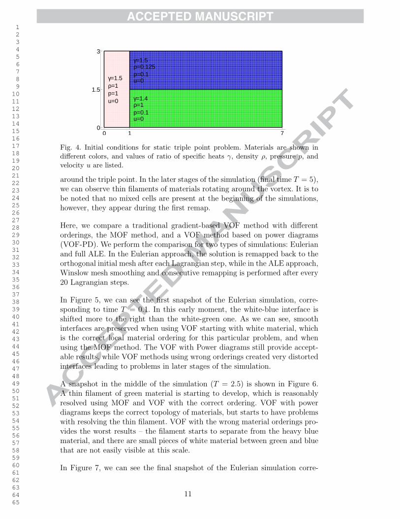
ACCEPTED MANUSCRIPT 1 2 3 4 5 6 7 8 9 10 11 12 13 14 15 16 17 18 19 20 21 22 23 24 25 26 27 28 29 30 31 32 33 34 35 36 37 38 39 40 41 42 43 44 45 46 47 48 49 50 51 52 53 54 55 56 57 58 59 60 61 62 63 64 65
0 1 70
1.5
3
γ=1.5ρ=1p=1u=0
γ=1.5ρ=0.125p=0.1u=0
γ=1.4ρ=1p=0.1u=0
Fig. 4. Initial conditions for static triple point problem. Materials are shown indifferent colors, and values of ratio of specific heats γ, density ρ, pressure p, andvelocity u are listed.
around the triple point. In the later stages of the simulation (final time T = 5),we can observe thin filaments of materials rotating around the vortex. It is tobe noted that no mixed cells are present at the beginning of the simulations,however, they appear during the first remap.
Here, we compare a traditional gradient-based VOF method with differentorderings, the MOF method, and a VOF method based on power diagrams(VOF-PD). We perform the comparison for two types of simulations: Eulerianand full ALE. In the Eulerian approach, the solution is remapped back to theorthogonal initial mesh after each Lagrangian step, while in the ALE approach,Winslow mesh smoothing and consecutive remapping is performed after every20 Lagrangian steps.
In Figure 5, we can see the first snapshot of the Eulerian simulation, corre-sponding to time T = 0.1. In this early moment, the white-blue interface isshifted more to the right than the white-green one. As we can see, smoothinterfaces are preserved when using VOF starting with white material, whichis the correct local material ordering for this particular problem, and whenusing the MOF method. The VOF with Power diagrams still provide accept-able results, while VOF methods using wrong orderings created very distortedinterfaces leading to problems in later stages of the simulation.
A snapshot in the middle of the simulation (T = 2.5) is shown in Figure 6.A thin filament of green material is starting to develop, which is reasonablyresolved using MOF and VOF with the correct ordering. VOF with powerdiagrams keeps the correct topology of materials, but starts to have problemswith resolving the thin filament. VOF with the wrong material orderings pro-vides the worst results – the filament starts to separate from the heavy bluematerial, and there are small pieces of white material between green and bluethat are not easily visible at this scale.
In Figure 7, we can see the final snapshot of the Eulerian simulation corre-
11

ACCEPTED MANUSCRIPT 1 2 3 4 5 6 7 8 9 10 11 12 13 14 15 16 17 18 19 20 21 22 23 24 25 26 27 28 29 30 31 32 33 34 35 36 37 38 39 40 41 42 43 44 45 46 47 48 49 50 51 52 53 54 55 56 57 58 59 60 61 62 63 64 65
0 2 4 60
1
2
3
Global view of MOF simulation
0.95 1 1.05 1.1 1.151.4
1.45
1.5
1.55
1.6
0.95 1 1.05 1.1 1.151.4
1.45
1.5
1.55
1.6
0.95 1 1.05 1.1 1.151.4
1.45
1.5
1.55
1.6
VOF – R first VOF – G first VOF – B first
0.95 1 1.05 1.1 1.151.4
1.45
1.5
1.55
1.6
0.95 1 1.05 1.1 1.151.4
1.45
1.5
1.55
1.6
MOF VOF-PD
Fig. 5. Materials of triple point problem simulation, time T = 0.1. Eulerian runs (asLagrangian step and remap to the initial orthogonal mesh) using different meth-ods for material reconstruction are shown: global view on the entire computationaldomain for MOF method, and zooms to the three material junction for Youngs’VOF method (with different material orderings), MOF, and Power Diagram basedmethods are shown.
sponding to time T = 5. Again, MOF and VOF in the correct ordering resolvethe thin part of the green filament reasonably well. VOF with the wrong ma-terial orderings give us unacceptable results – filament transforms into a dripseparating from the blue material, and there are many tiny droplets of whitematerial between the blue and green materials VOF with power diagrams alsodo not succeed in resolving the thin part of the filament, but the result isqualitatively better: the material topology is correct, no droplets appear, andgreen material stays attached to the blue one.
In the next set of figures, the results of the same problem obtained by ALE
12

ACCEPTED MANUSCRIPT 1 2 3 4 5 6 7 8 9 10 11 12 13 14 15 16 17 18 19 20 21 22 23 24 25 26 27 28 29 30 31 32 33 34 35 36 37 38 39 40 41 42 43 44 45 46 47 48 49 50 51 52 53 54 55 56 57 58 59 60 61 62 63 64 65
0 2 4 60
1
2
3
Global view of MOF simulation
2.8 3 3.2
1.4
1.5
1.6
1.7
1.8
2.8 3 3.2
1.4
1.5
1.6
1.7
1.8
2.8 3 3.2
1.4
1.5
1.6
1.7
1.8
VOF – R first VOF – G first VOF – B first
2.8 3 3.2
1.4
1.5
1.6
1.7
1.8
2.8 3 3.2
1.4
1.5
1.6
1.7
1.8
MOF VOF-PD
Fig. 6. Materials of triple point problem simulation, time T = 2.5. Eulerian runs (asLagrangian step and remap to the initial orthogonal mesh) using different meth-ods for material reconstruction are shown: global view on the entire computationaldomain for MOF method, and zooms to the three material junction for Youngs’VOF method (with different material orderings), MOF, and Power Diagram basedmethods are shown.
approach are presented. Generally, the results are worse than for the Euleriansimulations due to the distorted computational mesh.
In Figure 8, the early stages of an ALE simulation at time T = 0.1 are pre-sented for the same example. As we can see, the MOF results are best of allmethods being compared, the multi-material interface smoothly transitionsfrom the white-blue to the white-green interface and no major jumps appear.The results of VOF in correct ordering are comparable to the results of VOFwith power diagrams at this early stage. We can observe minor material jumpsand smoothness of the interface is violated. The worst results are clearly ob-
13

ACCEPTED MANUSCRIPT 1 2 3 4 5 6 7 8 9 10 11 12 13 14 15 16 17 18 19 20 21 22 23 24 25 26 27 28 29 30 31 32 33 34 35 36 37 38 39 40 41 42 43 44 45 46 47 48 49 50 51 52 53 54 55 56 57 58 59 60 61 62 63 64 65
0 2 4 60
1
2
3
Global view of MOF simulation
4.3 4.4 4.5 4.6 4.71.4
1.5
1.6
1.7
1.8
4.3 4.4 4.5 4.6 4.71.4
1.5
1.6
1.7
1.8
4.3 4.4 4.5 4.6 4.71.4
1.5
1.6
1.7
1.8
VOF – R first VOF – G first VOF – B first
4.3 4.4 4.5 4.6 4.71.4
1.5
1.6
1.7
1.8
4.3 4.4 4.5 4.6 4.71.4
1.5
1.6
1.7
1.8
MOF VOF-PD
Fig. 7. Materials of triple point problem simulation, time T = 5.0. Eulerian runs (asLagrangian step and remap to the initial orthogonal mesh) using different meth-ods for material reconstruction are shown: global view on the entire computationaldomain for MOF method, and zooms to the three material junction for Youngs’VOF method (with different material orderings), MOF, and Power Diagram basedmethods are shown.
tained by VOF methods using the wrong material orderings. The T-shape ofthe interface is completely violated and an unphysical wedge of white materialstarts to separate blue and green materials, leading to more severe problemsin later stages of the simulations.
Figure 9 presents results in the middle of the simulation (T = 2.5). In this timemoment, the (initially orthogonal) computational mesh is already relativelydistorted. As we can see, VOF in correct ordering resolves the longest greenfilament. Filament resolved by MOF is shorter, compact, with a relatively
14

ACCEPTED MANUSCRIPT 1 2 3 4 5 6 7 8 9 10 11 12 13 14 15 16 17 18 19 20 21 22 23 24 25 26 27 28 29 30 31 32 33 34 35 36 37 38 39 40 41 42 43 44 45 46 47 48 49 50 51 52 53 54 55 56 57 58 59 60 61 62 63 64 65
0 2 4 60
1
2
3
Global view of MOF simulation
0.95 1 1.05 1.1 1.151.4
1.45
1.5
1.55
1.6
0.95 1 1.05 1.1 1.151.4
1.45
1.5
1.55
1.6
0.95 1 1.05 1.1 1.151.4
1.45
1.5
1.55
1.6
VOF – R first VOF – G first VOF – B first
0.95 1 1.05 1.1 1.151.4
1.45
1.5
1.55
1.6
0.95 1 1.05 1.1 1.151.4
1.45
1.5
1.55
1.6
MOF VOF-PD
Fig. 8. Materials of triple point problem simulation, time T = 0.1. ALE runs (as La-grangian step and remap to the Winslow smoothed mesh after every 20 Lagrangiansteps) using different methods for material reconstruction are shown: global view onthe entire computational domain for MOF method, and zooms to the three materialjunction for Youngs’ VOF method (with different material orderings), MOF, andPower Diagram based methods are shown.
smooth interface. Power diagrams and VOF with wrong material orderingsdo not resolve the filament very well, but power diagrams surpass VOF withincorrect material order in material topology – no fragment of white and bluematerial appear on the other side of the green filament.
In Figure 10, we can see the last moment (T = 5) of the ALE simulation.MOF provides best result again – the filament is compact, relatively smooth,no separated tiny droplets are present. We can observe such small pieces forall VOF methods, even for correct ordering, where a tiny thin fiber of greenmaterial separates white-blue interface upto the picture boundary (zoomed in
15

ACCEPTED MANUSCRIPT 1 2 3 4 5 6 7 8 9 10 11 12 13 14 15 16 17 18 19 20 21 22 23 24 25 26 27 28 29 30 31 32 33 34 35 36 37 38 39 40 41 42 43 44 45 46 47 48 49 50 51 52 53 54 55 56 57 58 59 60 61 62 63 64 65
0 2 4 60
1
2
3
Global view of MOF simulation
2.8 3 3.2
1.4
1.5
1.6
1.7
1.8
2.8 3 3.2
1.4
1.5
1.6
1.7
1.8
2.8 3 3.2
1.4
1.5
1.6
1.7
1.8
VOF – R first VOF – G first VOF – B first
2.8 3 3.2
1.4
1.5
1.6
1.7
1.8
2.8 3 3.2
1.4
1.5
1.6
1.7
1.8
MOF VOF-PD
Fig. 9. Materials of triple point problem simulation, time T = 2.5. ALE runs (as La-grangian step and remap to the Winslow smoothed mesh after every 20 Lagrangiansteps) using different methods for material reconstruction are shown: global view onthe entire computational domain for MOF method, and zooms to the three materialjunction for Youngs’ VOF method (with different material orderings), MOF, andPower Diagram based methods are shown.
the last image of Figure 10). As for power diagrams, no droplets appear, butwe can see that the green filament has broken into two parts.
6.2 Multi-material Sedov problem
The second numerical problem we present here is a multi-material generaliza-tion of the well known Sedov problem [31]. Typically, only one quarter of theSedov problem is solved in the domain 〈0, 1.1〉2, final time of the simulation
16

ACCEPTED MANUSCRIPT 1 2 3 4 5 6 7 8 9 10 11 12 13 14 15 16 17 18 19 20 21 22 23 24 25 26 27 28 29 30 31 32 33 34 35 36 37 38 39 40 41 42 43 44 45 46 47 48 49 50 51 52 53 54 55 56 57 58 59 60 61 62 63 64 65
0 2 4 60
1
2
3
Global view of MOF simulation
4.3 4.4 4.5 4.6 4.71.4
1.5
1.6
1.7
1.8
4.3 4.4 4.5 4.6 4.71.4
1.5
1.6
1.7
1.8
4.3 4.4 4.5 4.6 4.71.4
1.5
1.6
1.7
1.8
VOF – R first VOF – G first VOF – B first
4.3 4.4 4.5 4.6 4.71.4
1.5
1.6
1.7
1.8
4.3 4.4 4.5 4.6 4.71.4
1.5
1.6
1.7
1.8
4.2 4.3 4.4 4.51.65
1.7
1.75
1.8
1.85
1.9
MOF VOF-PD VOF – R, zoom
Fig. 10. Materials of triple point problem simulation, time T = 5.0. ALE runs (as La-grangian step and remap to the Winslow smoothed mesh after every 20 Lagrangiansteps) using different methods for material reconstruction are shown: global view onthe entire computational domain for MOF method, and zooms to the three materialjunction for Youngs’ VOF method (with different material orderings), MOF, andPower Diagram based methods are shown. A filament of green material for Youngs’VOF method with the correct material ordering is zoomed in the last image.
is T = 1. The standard Sedov problem has a uniform density ρ = 1, pressurep = 10−6, and ratio of specific heats γ = 1.4, the fluid is static. A high en-ergy cell in the domain origin is set, causing an explosion generating a strongcircular shock wave spreading from the origin.
In our modification, we paint 4 materials over the Cartesian computationalmesh containing 322 cells in the domain, as shown in Figure 11. The material
17

ACCEPTED MANUSCRIPT 1 2 3 4 5 6 7 8 9 10 11 12 13 14 15 16 17 18 19 20 21 22 23 24 25 26 27 28 29 30 31 32 33 34 35 36 37 38 39 40 41 42 43 44 45 46 47 48 49 50 51 52 53 54 55 56 57 58 59 60 61 62 63 64 65
0 0.2 0.4 0.6 0.8 10
0.2
0.4
0.6
0.8
1
AB
C
D
Fig. 11. Initial placement of materials for the multi-material Sedov problem paintedonto a Cartesian 322 mesh. The material interfaces are placed at radiuses r = 0.1,r = 0.2, and r = 0.3.
interfaces are placed at radiuses r = 0.1, r = 0.2, and r = 0.3. The centralmaterial A represents the high-energy (and also high-density) material gener-ating the explosion, its values are ρ = 10, p = 163.88, and γ = 1.4. The ring Bhas a very low density ρ = 0.2 and a very high ratio of specific heats γ = 50,which is the simplest approach for approximating a low-compressibility mate-rial. Pressure in ring B is p = 10−6. The fluid values in the high-density ringC are ρ = 5, p = 10−6, and γ = 5/3. Finally, in the rest of the domain D, thefluid values correspond to the values of a standard Sedov problem describedbefore.
After the simulation starts, the explosion-generated shock wave compressesthe low-density material B. As the density of the outer ring C is high, it hashigh momentum and is difficult to start moving, which causes even strongercompression of B. As the fluid moves outward from the explosion, materialB is being extended. Due to its high γ, the material gets thiner instead ofdecreasing of its density. At the end of the simulation, the thickness of ring Bchanges to about 20% of its original thickness.
The simulation results for different material reconstruction methods using anALE approach performing Winslow mesh smoothing and quantity remapping
18

ACCEPTED MANUSCRIPT 1 2 3 4 5 6 7 8 9 10 11 12 13 14 15 16 17 18 19 20 21 22 23 24 25 26 27 28 29 30 31 32 33 34 35 36 37 38 39 40 41 42 43 44 45 46 47 48 49 50 51 52 53 54 55 56 57 58 59 60 61 62 63 64 65
after every 10 Lagrangian steps are presented in Figure 12. For the Youngs’
0 0.2 0.4 0.6 0.8 10
0.2
0.4
0.6
0.8
1
0 0.2 0.4 0.6 0.8 10
0.2
0.4
0.6
0.8
1
VOF MOF
0 0.2 0.4 0.6 0.8 10
0.2
0.4
0.6
0.8
1
VOF-PD
Fig. 12. Materials of multi-material Sedov problem, time T = 1, 322 mesh. ALEruns (as Lagrangian step and remap to the Winslow smoothed mesh after every 10Lagrangian steps) using different methods for material reconstruction are shown:material interfaces for Youngs’ VOF (in ABCD order), MOF, and Power Diagrambased methods are shown.
VOF method, the ABCD ordering is used, which is considered to be correctfor this problem (generally, for problems including layered structures, the or-dering following the materials from one side to the other one is correct). Evenso, the Youngs’ VOF methods produces the worst results, and the blue ring Bis broken at several places. As we can see, the severest material displacementis present at domain boundaries due to the distortion of the volume fractiongradient here. Although, we can also observe fragments of the green materialbetween the red and blue ones along the whole blue ring. For MOF, the bluering stays compact with smooth interfaces. For this problem, the results ob-
19

ACCEPTED MANUSCRIPT 1 2 3 4 5 6 7 8 9 10 11 12 13 14 15 16 17 18 19 20 21 22 23 24 25 26 27 28 29 30 31 32 33 34 35 36 37 38 39 40 41 42 43 44 45 46 47 48 49 50 51 52 53 54 55 56 57 58 59 60 61 62 63 64 65
tained by the Power Diagrams based VOF method are comparable to MOFresults, with the exception of the inner material interface disturbances closeto the domain boundary. These are again caused by the computation of thevolume fraction gradient. Let us note, that the circular shock wave positionis the same and is not influenced by the particular material reconstructionmethod.
6.3 Multi-material Saltzman-like Problem
The last problem we are going to discuss here is a modification of a stan-dard Saltzman piston problem [32]. We use an orthogonal Cartesian 100× 10computational mesh in the computational domain 〈−0.5, 0.5〉× 〈−0.05, 0.05〉.The standard Saltzman problem contains a uniform distribution of materialdensity ρ = 1 and pressure p = 2/3 · 10−4 in the whole domain. The fluid isstatic and the ratio of specific heats is γ = 5/3. After the beginning of thesimulation, the whole computational domain is compressed by a piston mov-ing the left boundary with the unit velocity. As the simulations goes, a shockwave is formed in front of the piston, which passes the whole domain andreflects from the right boundary. It is possible to perform this simulation untilquite a long time, when the shock wave reflects several times from the left andright boundaries. Let us note, that in time T = 1, the whole domain would becompressed to the 0 width, so this time is not reachable. This problem is oftenused for the investigation of the properties of Lagrangian solvers, especiallywhen used in connection with an initially skewed computational mesh.
In our modification, we have placed several rings of different materials to thecenter of the computational domain, as can be seen in Figure 13. The ra-
−0.5 −0.4 −0.3 −0.2 −0.1 0 0.1 0.2 0.3 0.4 0.5−0.05
0
0.05A B C D
Fig. 13. Initial placement of materials for the multi-material Saltzman problempainted onto a Cartesian 100 × 10 mesh. The material interfaces are placed to theradiuses r = 0.02, r = 0.027, and r = 0.03.
diuses of the material interfaces are set to r = 0.02, r = 0.027, and r = 0.03.This problem is multi-material only formally, the fluid quantities of all mate-rials are set to the same values as mentioned above. Therefore, the solutionshould exactly correspond to the 1D symmetric solution of the single-materialproblem.
In Figure 14, we can see the comparison of the Youngs’ VOF, VOF-PD, and
20

ACCEPTED MANUSCRIPT 1 2 3 4 5 6 7 8 9 10 11 12 13 14 15 16 17 18 19 20 21 22 23 24 25 26 27 28 29 30 31 32 33 34 35 36 37 38 39 40 41 42 43 44 45 46 47 48 49 50 51 52 53 54 55 56 57 58 59 60 61 62 63 64 65
−0.03 −0.02 −0.01 0 0.01 0.02 0.03
−0.03
−0.02
−0.01
0
0.01
0.02
0.03
−0.03 −0.02 −0.01 0 0.01 0.02 0.03
−0.03
−0.02
−0.01
0
0.01
0.02
0.03
−0.03 −0.02 −0.01 0 0.01 0.02 0.03
−0.03
−0.02
−0.01
0
0.01
0.02
0.03
100 × 10, VOF 100 × 10, VOF-PD 100 × 10, MOF
−0.03 −0.02 −0.01 0 0.01 0.02 0.03
−0.03
−0.02
−0.01
0
0.01
0.02
0.03
−0.03 −0.02 −0.01 0 0.01 0.02 0.03
−0.03
−0.02
−0.01
0
0.01
0.02
0.03
−0.03 −0.02 −0.01 0 0.01 0.02 0.03
−0.03
−0.02
−0.01
0
0.01
0.02
0.03
200 × 20, VOF 200 × 20, VOF-PD 200 × 20, MOF
−0.03 −0.02 −0.01 0 0.01 0.02 0.03
−0.03
−0.02
−0.01
0
0.01
0.02
0.03
−0.03 −0.02 −0.01 0 0.01 0.02 0.03
−0.03
−0.02
−0.01
0
0.01
0.02
0.03
−0.03 −0.02 −0.01 0 0.01 0.02 0.03
−0.03
−0.02
−0.01
0
0.01
0.02
0.03
400 × 40, VOF 400 × 40, VOF-PD 400 × 40, MOF
−0.03 −0.02 −0.01 0 0.01 0.02 0.03
−0.03
−0.02
−0.01
0
0.01
0.02
0.03
−0.03 −0.02 −0.01 0 0.01 0.02 0.03
−0.03
−0.02
−0.01
0
0.01
0.02
0.03
−0.03 −0.02 −0.01 0 0.01 0.02 0.03
−0.03
−0.02
−0.01
0
0.01
0.02
0.03
800 × 80, VOF 800 × 80, VOF-PD 800 × 80, MOF
Fig. 14. Multi-material Saltzman problem in time T = 0 on a Cartesian meshes withdifferent resolutions. The computational mesh and material polygons reconstructedby the different reconstruction methods in the ring regions are shown.
21

ACCEPTED MANUSCRIPT 1 2 3 4 5 6 7 8 9 10 11 12 13 14 15 16 17 18 19 20 21 22 23 24 25 26 27 28 29 30 31 32 33 34 35 36 37 38 39 40 41 42 43 44 45 46 47 48 49 50 51 52 53 54 55 56 57 58 59 60 61 62 63 64 65
MOF material reconstruction methods applied to the initial data of the de-scribed problem. For the Youngs’ VOF methods, the ABCD material order-ing was used, considered to the correct ordering for layered structures. Theproblem uses 100 × 10, 200 × 20, 400 × 40, and 800 × 80 mesh resolutions,in the images a zoom of the ring region is shown. For the lowest resolution,the problem is clearly under-resolved. We can observe severe distortions ofthe green ring due to inaccurate gradient computation. The gradient is com-puted by the Green-Gauss approach, and the stencil of the surrounding cellsincluding the green material is not big enough for the filament structure toresolve the gradient accurately. We can even see pieces of the green materialbetween the light-red and blue materials. The VOF-PD and MOF methodskeep the material topology correctly, but the MOF method produces muchsmoother interfaces. The reason for non-smooth VOF-PD interfaces are thesame as for the Youngs’ VOF method – inaccurate gradient computation. Forthe 200× 20 mesh, the situation is similar. We can still observe perturbancesof the green ring material due to the inaccurate gradient computation. TheMOF and VOF-PD results are now comparable, all interfaces are smooth. Forthe 400 × 40 mesh, few tiny magenta pieces can still be found between theblue and green rings in the case of VOF method. This can be seen in thezoom shown in Figure 15. Finally, for the highest resolution mesh 800×80, all
−0.022 −0.021 −0.02 −0.019 −0.018 −0.0170.017
0.0175
0.018
0.0185
0.019
0.0195
0.02
0.0205
0.021
Fig. 15. Multi-material Saltzman problem in time T = 0 on a Cartesian 400 × 40mesh. The computational mesh and material polygons reconstructed by the VOFreconstruction method are shown. Zoom shows fragments of the magenta material.
material features are at least 3 cells wide and all methods provide comparableresults with smooth interfaces and correct material topology.
22

ACCEPTED MANUSCRIPT 1 2 3 4 5 6 7 8 9 10 11 12 13 14 15 16 17 18 19 20 21 22 23 24 25 26 27 28 29 30 31 32 33 34 35 36 37 38 39 40 41 42 43 44 45 46 47 48 49 50 51 52 53 54 55 56 57 58 59 60 61 62 63 64 65
Let us also note, that the problems with the Youngs’ VOF method could beimproved in this particular problem by changing the material ordering suchthat the thin green filament would be treated as last. As we have already said,generally for layered structures, the ordering respecting the ordering of thelayers is considered as correct and used in most simulations. Moreover, this fixis not applicable if there would be two or more filaments next to each other.
We perform the simulation of the multi-material Saltzman-like problem tillthe (quite an early) final time T = 0.6, in which the shock wave passes therings for the first time, as can be seen for the case of MOF method on the100×10 mesh in Figure 16. As we can see, in this time the piston has reached
0.1 0.15 0.2 0.25 0.3 0.35 0.4 0.45 0.5−0.05
0
0.05
Fig. 16. Multi-material Saltzman problem in time T = 0.6 on a Cartesian 100 × 10mesh obtained by the ALE1 simulation (Winslow mesh smoothing followed by thequantity remapping is performed after every single Lagrangian step). The com-putational mesh and material polygons reconstructed by the MOF reconstructionmethod are shown.
the position 0.1, the shock position is about 0.3. The left part of the domain(the part behind the shock wave, including the rings) is compressed and thecomputational cells have the aspect ratio of about 1/4. A zoom of the ringregion is shown in Figure 17.
For comparison of different material reconstruction methods, see Figure 18.The images show zooms to the ring regions, the aspect ratio is not preservedhere. As in Figure 14, the ABCD material ordering was used for the Youngs’VOF method. For the lowest 100 × 10 mesh resolution, both VOF and VOF-PD produce very bad results. VOF-PD surpasses the Youngs’ VOF methodslightly – the blue and green rings are mixed together, but stays relatively wellseparated from the background magenta material, contrary to the Youngs’VOF method for which all these three materials are mixed together. Theproblems of Youngs’ VOF start in the very early stages of the simulations, aswe saw in Figure 14. We can observe severe distortions of the thin green ringdue to the Green-Gauss computation of the material volume fraction gradientin the coarse mesh. Despite the coarseness of the mesh the MOF result issuperior. For the finer 200×20 computational mesh, the Youngs’ VOF method(with the correct material ordering) is the worst – the green ring is completelydistorted, and we can see small pieces of the green and magenta materials
23

ACCEPTED MANUSCRIPT 1 2 3 4 5 6 7 8 9 10 11 12 13 14 15 16 17 18 19 20 21 22 23 24 25 26 27 28 29 30 31 32 33 34 35 36 37 38 39 40 41 42 43 44 45 46 47 48 49 50 51 52 53 54 55 56 57 58 59 60 61 62 63 64 65
0.22 0.225 0.23
−0.03
−0.02
−0.01
0
0.01
0.02
0.03
Fig. 17. Zoom-in of the multi-material Saltzman problem in time T = 0.6 on aCartesian 100× 10 mesh obtained by the ALE1 simulation (Winslow mesh smooth-ing followed by the quantity remapping is performed after every single Lagrangianstep). The computational mesh and material polygons reconstructed by the MOFreconstruction method are shown.
on the blue-light red interface. The VOF-PD result is significantly better, thegreen ring is much more compact, but still small pieces of the magenta and bluematerials can be found inside the left and right parts of the green circle. ForMOF, all materials stay compact and no problems with the tiny material piecesappear. In the case of 400 × 40 mesh resolution, the VOF method provides
24

ACCEPTED MANUSCRIPT 1 2 3 4 5 6 7 8 9 10 11 12 13 14 15 16 17 18 19 20 21 22 23 24 25 26 27 28 29 30 31 32 33 34 35 36 37 38 39 40 41 42 43 44 45 46 47 48 49 50 51 52 53 54 55 56 57 58 59 60 61 62 63 64 65
0.218 0.22 0.222 0.224 0.226 0.228 0.23 0.232 0.234
−0.03
−0.02
−0.01
0
0.01
0.02
0.03
0.218 0.22 0.222 0.224 0.226 0.228 0.23 0.232 0.234
−0.03
−0.02
−0.01
0
0.01
0.02
0.03
0.218 0.22 0.222 0.224 0.226 0.228 0.23 0.232 0.234
−0.03
−0.02
−0.01
0
0.01
0.02
0.03
100 × 10, VOF 100 × 10, VOF-PD 100 × 10, MOF
0.218 0.22 0.222 0.224 0.226 0.228 0.23 0.232 0.234
−0.03
−0.02
−0.01
0
0.01
0.02
0.03
0.218 0.22 0.222 0.224 0.226 0.228 0.23 0.232 0.234
−0.03
−0.02
−0.01
0
0.01
0.02
0.03
0.218 0.22 0.222 0.224 0.226 0.228 0.23 0.232 0.234
−0.03
−0.02
−0.01
0
0.01
0.02
0.03
200 × 20, VOF 200 × 20, VOF-PD 200 × 20, MOF
0.218 0.22 0.222 0.224 0.226 0.228 0.23 0.232 0.234
−0.03
−0.02
−0.01
0
0.01
0.02
0.03
0.218 0.22 0.222 0.224 0.226 0.228 0.23 0.232 0.234
−0.03
−0.02
−0.01
0
0.01
0.02
0.03
0.218 0.22 0.222 0.224 0.226 0.228 0.23 0.232 0.234
−0.03
−0.02
−0.01
0
0.01
0.02
0.03
400 × 40, VOF 400 × 40, VOF-PD 400 × 40, MOF
0.218 0.22 0.222 0.224 0.226 0.228 0.23 0.232 0.234
−0.03
−0.02
−0.01
0
0.01
0.02
0.03
0.218 0.22 0.222 0.224 0.226 0.228 0.23 0.232 0.234
−0.03
−0.02
−0.01
0
0.01
0.02
0.03
0.218 0.22 0.222 0.224 0.226 0.228 0.23 0.232 0.234
−0.03
−0.02
−0.01
0
0.01
0.02
0.03
800 × 80, VOF 800 × 80, VOF-PD 800 × 80, MOF
Fig. 18. Multi-material Saltzman problem in time T = 0.6 on a Cartesian mesheswith different resolutions, obtained by the ALE1 simulation (Winslow mesh smooth-ing followed by the quantity remapping is performed after every single Lagrangianstep). The computational mesh and material polygons reconstructed by the differentreconstruction methods in the ring regions are shown.
25

ACCEPTED MANUSCRIPT 1 2 3 4 5 6 7 8 9 10 11 12 13 14 15 16 17 18 19 20 21 22 23 24 25 26 27 28 29 30 31 32 33 34 35 36 37 38 39 40 41 42 43 44 45 46 47 48 49 50 51 52 53 54 55 56 57 58 59 60 61 62 63 64 65
better results than in the lower resolutions, but there are still fragments ofthe magenta material between the green and blue rings. We do not observeany material topology problems with VOF-PD or MOF method. Finally, thesame set of simulations was performed on the finest 800 × 80 mesh. As wecan see, even the thinnest green ring is now about 3 cells wide. This allowan exact computation of the gradient of the volume fractions functions, andso the final materials are smooth, compact, and comparable to the results ofthe MOF method. Similarly, VOF-PD results are comparable to MOF results,materials are smooth, and no problems with material topology are visible. Aswe can see, all methods converge towards the same material distribution asthe mesh refines.
7 Conclusions
We have presented a comparison of a material-order-dependent VOF method,a material-order-independent VOF method and a material-order-independentMOF method for a complex compressible flow involving more than two mate-rials.
From the simulations that we have run, we conclude that:
• MOF performs the most accurate reconstructions, generally capturing fil-aments accurately and getting the material topology correct. Since MOFis quite recent it generally does not exist in many codes. Therefore, thismethod is the best choice when developing new flow codes or when revamp-ing the interface tracking machinery. It is not advisable to introduce MOFreconstruction into a flow code without ensuring that the advection (remap-ping) of centroids is done accurately through overlays (exact, intersection-based remapping method).
• VOF with the correct material order performs remarkably well althoughthe resolution of filaments and other small features is poorer than MOF.Since VOF commonly exists in flow codes that perform this type of interfacetracking, it is a natural choice when the flow is simple and the material ordercan be predicted quite easily. It is also a good choice when the flow has onlytwo materials and no filamentary or other structures smaller than 3-4 timesthe grid resolution are expected.
• Compared to VOF, the MOF method is less efficient. As it was alreadymentioned, all possible material combinations are tested to find the optimalmaterial placement. If the number of materials in one cell would happen tobe high (more than 5) in many cells, the MOF method could represent aconsiderable computational cost of the simulation. Fortunately, in the usualsimulations, this situation is very rare – typically, there are many 2-materialcells, some 3-material cells, and just a few 4 or more -material cells.
26

ACCEPTED MANUSCRIPT 1 2 3 4 5 6 7 8 9 10 11 12 13 14 15 16 17 18 19 20 21 22 23 24 25 26 27 28 29 30 31 32 33 34 35 36 37 38 39 40 41 42 43 44 45 46 47 48 49 50 51 52 53 54 55 56 57 58 59 60 61 62 63 64 65
• VOF with power diagrams performs more poorly than MOF or VOF withthe right material order but usually gets the interface topology right. Thismethod is a good choice when the advection machinery cannot be revampedto perform overlays but the interface reconstruction can be rewritten simplyto partition cells using the power diagram.
• VOF with the wrong order performs poorly even for simple flows and is notadvised. If the ordering cannot be predicted or enforced strictly, it is betterto use VOF with the power diagram reconstruction.
A Appendix
A.1 Lagrangian update of material centroids
The Lagrangian step may be viewed as the implicit creation of a family ofmaps, φn(x) : R
d 7→ Rd, such that xn+1 = φn+1(xn). Any material region,
Ωt ⊂ Rd, evolves over a time step as
Ωn+1 = φn+1(Ωn) (A.1)
The map φn+1 is illustrated in Figure A.1.
If the map is an affine transformation, that is
φn+1(x) = Ax + b (A.2)
where A ∈ Rd×d is invertible and b ∈ R
d, then if xc(Ωn) is the centroid of
the region and Ωn+1 = φn+1(Ωn), then xc(Ωn+1) = Axc(Ω
n) + b. That is, thetransformed centroid is the centroid of the transformed region.
To demonstrate this,
‖Ωn+1‖xc(Ωn+1)=
∫Ωn+1
x dx
=∫Ωn
(Ay + b) detA dy
= (detA)‖Ωn‖Axc(Ωn) + b(detA)‖Ωn‖
Noting that
‖Ωn+1‖ =∫Ωn+1
dx =∫Ωn
detA dx = ‖Ωn‖ detA
we obtain,xc(Ω
n+1) = Axc(Ωn) + b
27

ACCEPTED MANUSCRIPT 1 2 3 4 5 6 7 8 9 10 11 12 13 14 15 16 17 18 19 20 21 22 23 24 25 26 27 28 29 30 31 32 33 34 35 36 37 38 39 40 41 42 43 44 45 46 47 48 49 50 51 52 53 54 55 56 57 58 59 60 61 62 63 64 65
The actual Lagrangian evolution of the region is given by the pointwise equa-tion
dx
dt= u(x, t) ∀x ∈ Ωt (A.3)
assuming the velocity field is known. The transformation, φn+1, is then thesolution to Equation A.3 over the time interval [tn, tn+1].
With sufficient regularity, the velocity field can be expanded as
uj(x, t) = uj(x0, tn) + (t− tn)
∂uj(x0, tn)
∂t+ (xi − x0
i )∂uj(x0, t
n)
∂xi
+O(∆x2) + O(∆t2) + O(∆x∆t).(A.4)
Substituting this into Equation A.3 and integrating, we find that
φn+1(x) = x + u(x0, tn)∆t+ O(∆t2) + O(∆t∆x). (A.5)
Assuming ∆t ≈ ∆x, then the transformation defining the Lagrangian evolu-tion over a time step may be approximated as an affine transformation withsecond order accuracy.
A.2 Constant parametric coordinate method
A method for updating material centroids during a Lagrangian step can exploitthis implicit evolution operator described above. The method described [2,19]is based on the existence of a mapping of the computational cell to and froma logical space. It is assumed that the centroid of the material region has thesame logical coordinates, before and after the Lagrangian motion of the cell.To obtain the centroid after the Lagrangian motion, the logical coordinates ofthe centroid at the previous step are given to the logical to physical mappingcorresponding to the cell after the motion. This process is illustrated in FigureA.1. It is important to note that the logical to physical space mapping isdifferent for each time step and the cells evolve in time.
The accuracy of the method relies on the properties of the logical to physicalcoordinate transformations used.
Assume each cell has local coordinates, r ∈ S, with an invertible map intophysical coordinates, ψn : S 7→ Ωn.
We define a family of local parameterizations, ψn to be linearity preserv-ing, if points from the parametric space, S, are mapped such that if
xn+1 = Axn + b, (A.6)
28

ACCEPTED MANUSCRIPT 1 2 3 4 5 6 7 8 9 10 11 12 13 14 15 16 17 18 19 20 21 22 23 24 25 26 27 28 29 30 31 32 33 34 35 36 37 38 39 40 41 42 43 44 45 46 47 48 49 50 51 52 53 54 55 56 57 58 59 60 61 62 63 64 65
tn
xn0 xn
1
xn2
xn3
xc(Ωn) (1)
(ψn)−1(xc(Ωn))
rn0 rn
1
rn2rn
3
rc
(2) I : S 7→ S
tn+1
rn0 rn
1
rn2rn
3
rc
(3)
ψn+1(rc)
Ωn+1 = φn+1(Ωn)
xn+10
xn+11
xn+12xn+1
3
xc(Ωn+1)
Fig. A.1. Steps in the constant parametric coordinate method. (1) The logical coor-dinates of the centroid at time tn are calculated. (2) It is assumed the centroid hasthe same logical coordinates at time tn+1. (3) The logical coordinates are mappedto physical coordinates to give the location. This gives a second order accurateapproximation to the centroid of the evolved region Ωn+1 = φn+1(Ωn).
then if xn = ψn(r),
xn+1 = ψn+1(r) = Aψn(r) + b = Axn + b (A.7)
Equivalently,
ψn+1 = Aψn + b (A.8)
The bilinear parameterization of quads satisfies this property: the two orthog-onal coordinates, (r, s) ∈ [0, 1]2 linearly interpolate the vertices (see FigureA.1 for node numbering)
ψn(r, s) = (1 − r) [(1 − s)xn0 + sxn
3 ] + r [(1 − s)xn1 + sxn
2 ] (A.9)
Clearly, ψn+1 = Aψn + b as xjn+1 = Axj
n + b for j = 0, . . . , 3.
The generalized barycentric coordinates of polygon with vertices vi alsosatisfies the linearity preserving property. To demonstrate this, barycentriccoordinates satisfy the properties [33],
29

ACCEPTED MANUSCRIPT 1 2 3 4 5 6 7 8 9 10 11 12 13 14 15 16 17 18 19 20 21 22 23 24 25 26 27 28 29 30 31 32 33 34 35 36 37 38 39 40 41 42 43 44 45 46 47 48 49 50 51 52 53 54 55 56 57 58 59 60 61 62 63 64 65
x=∑
i
λivi = ψn(λ), (A.10)
∑i
λi = 1, (A.11)
λi ≥ 0. (A.12)
If x has barycentric coordinates λ, then if xn = ψn(λ),
Ax=∑
i
λiAvi (A.13)
Aψn(λ) + b=∑
i
λiAvi + b∑
i
λi (A.14)
Aψn(λ) + b=∑
i
λi(Avi + b) = ψn+1(λ) (A.15)
where∑
i λi = 1 was utilized in the second step.
If the family of transformations satisfy the linearity preserving property, thenwe may analyze the accuracy of the constant parametric coordinate method.If the parameterization family, ψn, is linearity preserving, then updatingthe location of a material centroid by assuming its parametric coordinatesare unchanged is exact for linear motions, since for an arbitrary subdomainmapped with an affine transformation,
xc(Ωn+1) = Axc(Ω
n) + b (A.16)
If the transformation is linearity preserving, then
xc(Ωn+1) = ϕn+1(r) = Aϕn(r) + b = Axc(Ω
n) + b (A.17)
In general, the Lagrangian motion will not be linear. However, as was shown inthe previous section, for sufficient regularity in time an affine approximationto the Lagrangian motion is second order accurate.
Acknowledgments
This work was performed under the auspices of the National Nuclear Secu-rity Administration of the US Department of Energy at Los Alamos NationalLaboratory under Contract No. DE-AC52-06NA25396 and supported by theDOE Advanced Simulation and Computing (ASC) program. The authors ac-knowledge the partial support of the DOE Office of Science ASCR Program.
30

ACCEPTED MANUSCRIPT 1 2 3 4 5 6 7 8 9 10 11 12 13 14 15 16 17 18 19 20 21 22 23 24 25 26 27 28 29 30 31 32 33 34 35 36 37 38 39 40 41 42 43 44 45 46 47 48 49 50 51 52 53 54 55 56 57 58 59 60 61 62 63 64 65
References
[1] Benson DJ. Computational methods in Lagrangian and Eulerian hydrocodes.Computer Methods in Applied Mechanics and Engineering 1992; 99: 235-394.
[2] Benson DJ. Volume of fluid interface reconstruction methods for multi-materialproblems. Applied Mechanics Review 2002; 55(2): 151-165.
[3] Rider WJ, Kothe DB. Reconstructing volume tracking. Journal ofComputational Physics 1998; 141: 112-152.
[4] Scardovelli R, Zaleski S. Direct numerical simulation of free-surface andinterfacial flow. Annual Review of Fluid Mechanics 1999; 31: 567-603.
[5] Hirt CW, Nichols BD. Volume of fluid (VOF) method for the dynamics of freeboundaries. Journal of Computational Physics 1981; 39: 201-225.
[6] Dyadechko V, Shashkov MJ. Reconstruction of multi-material interfaces frommoment data. Journal of Computational Physics, 2008; 11: 5361-5384.
[7] Noh WF, Woodward P. SLIC (simple line interface calculation). In van derVooren AI and Zandbergen PJ, editors, 5th International Conference onNumerical Methods in Fluid Dynamics, pages 330-340. Springer-Verlag, 1976.
[8] Youngs DL. Time dependent multi-material flow with large fluid distortion.In K. W. Morton and M. J. Baines, editors, Numerical Methods for FluidDynamics, pages 273-285. Academic Press, 1982.
[9] Youngs DL. An interface tracking method for a 3D Eulerian hydrodynamicscode. Technical Report AWE/44/92/35, AWRE Design and Math Division,1984.
[10] Pilliod JE Jr., Puckett EG. Second-order accurate volume-of-fluid algorithmsfor tracking material interfaces. Journal of Computational Physics 2004; 199:465-502.
[11] Swartz BK. The second-order sharpening of blurred smooth borders.Mathematics of Computation 1989; 52(186): 675-714.
[12] Steinhaus H. A note on the ham sandwich theorem Mathesis Polska, 1938; 9:26-28.
[13] Stone AH, Tukey JW. Generalized “sandwich” theorems Duke MathematicalJournal, 1942; 9: 356-359.
[14] Mosso S, Clancy S. A geometrically derived priority system for Young’s interfacereconstruction. Technical Report LA-CP-95-0081, Los Alamos NationalLaboratory, Los Alamos, NM, 1995.
[15] Garimella RV, Dyadechko V, Swartz BK, Shaskov MJ. Interface reconstructionin multi-fluid, multi-phase flow simulations. In Proceedings of the 14thInternational Meshing Roundtable, pages 19-32, San Diego, CA, September2005. Springer.
31

ACCEPTED MANUSCRIPT 1 2 3 4 5 6 7 8 9 10 11 12 13 14 15 16 17 18 19 20 21 22 23 24 25 26 27 28 29 30 31 32 33 34 35 36 37 38 39 40 41 42 43 44 45 46 47 48 49 50 51 52 53 54 55 56 57 58 59 60 61 62 63 64 65
[16] Schofield SP, Garimella RV, Francois MM, Loubere R. Material order-independent interface reconstruction using power diagrams InternationalJournal for Numerical Methods in Fluids, 2007; 56(6): 643-659.
[17] Ahn HT, Shashkov M. Multi-material interface reconstruction on generalizedpolyhedral meshes. Journal of Computational Physics 2007; 226: 2096-2132.
[18] Schofield SP, Garimella RV, Francois MM, Loubere R. A second-orderaccurate material-order-independent interface reconstruction technique formulti-material flow simulations Journal of Computational Physics, 2009;228(3): 731-745.
[19] Benson DJ. Eulerian finite element methods for the micromechanicsof heterogeneous materials: Dynamic prioritization of material interfaces.Computer Methods in Applied Mechanics and Engineering, 1998, 151: 343-360.
[20] Aurenhammer F. Power diagrams: properties, algorithms and applications.SIAM J. Computing 1987; 16(1): 78-96.
[21] Imai H, Iri M, Murota K. Voronoi diagram in the Laguerre geometry and itsapplications. SIAM J. Computing 1985; 14(1): 93-105.
[22] Caramana EJ, Burton DE, Shashkov MJ, Whalen PP. The construction ofcompatible hydrodynamics algorithms utilizing conservation of total energy.Journal of Computational Physics 1998; 146: 227-262.
[23] Caramana EJ, Shashkov MJ, Whalen PP. Formulations of artificial viscosity formuti-dimensional shock wave computations. Journal of Computational Physics1998; 144: 70-97.
[24] Scovazzi G, Love E, Shashkov M. Multi-scale Lagrangian shock hydrodynamicson Q1/P0 finite elements: Theoretical framework and two-dimensionalcomputations. Comput. Methods Appl. Mech. Engrg. 2008; 197: 1056-1079.
[25] Shashkov M. Closure models for multidimensional cells in arbitrary Lagrangian-Eulerian hydrocodes. Int. J. Numer. Meth. Fluids 2008; 56: 1497-1504.
[26] Winslow AM. Equipotential zoning of two-dimensional meshes. TechnicalReport UCRL-7312, Lawrence Livermore National Laboratory, 1963.
[27] Margolin LG, Shashkov M. Second-order sign-preserving conservativeinterpolation (remapping) on general grids. Journal of Computational Physics2003; 184: 266-298.
[28] Pember RB, Anderson RW. A comparison of staggered-mesh Lagrange plusremap and cell-centered direct Eulerian Godunov schemes for Eulerian shockhydrodynamics. Technical Report UCRL-JC-139820, Lawrence LivermoreNational Laboratory, 2000.
[29] Kucharik M, Shashkov M. Conservative Multi-Material Remap for StaggeredDiscretization. In preparation 2009.
[30] Maire P-H. Personal Communication. Los Alamos National Laboratory, 2007.
32

ACCEPTED MANUSCRIPT 1 2 3 4 5 6 7 8 9 10 11 12 13 14 15 16 17 18 19 20 21 22 23 24 25 26 27 28 29 30 31 32 33 34 35 36 37 38 39 40 41 42 43 44 45 46 47 48 49 50 51 52 53 54 55 56 57 58 59 60 61 62 63 64 65
[31] Sedov LI. Similarity and Dimensional Methods in Mechanics. Academic Press,1959.
[32] Dukowicz JK, Meltz BJA. Vorticity errors in multidimensional Lagrangiancodes. Journal of Computational Physics, 1992; 99(1): 115-134.
[33] J. Warren, S. Schaefer, A. N. Hirani, and M. Desbrun. Barycentric coordinatesfor convex sets. Advances in Computational Mathematics, 2007; 27(3): 319-338.
33