Accounting for Biases in Black-Scholes∗

David Backus,† Silverio Foresi,‡ and Liuren Wu§

First draft: August 3, 1997This version: August 31, 2004

Abstract

Prices of currency options commonly differ from the Black-Scholes formula along twodimensions: implied volatilities vary by strike price (volatility smiles) and maturity(implied volatility of at-the-money options increases, on average, with maturity).We account for both using Gram-Charlier expansions to approximate the conditionaldistribution of the logarithm of the price of the underlying security. In this setting,volatility is approximately a quadratic function of moneyness, a result we use to inferskewness and kurtosis from volatility smiles. Evidence suggests that both kurtosisin currency prices and biases in Black-Scholes option prices decline with maturity.

JEL Classification Codes: G12, G13, F31, C14.

Keywords: currency options; skewness and kurtosis; Gram-Charlier expansions;implied volatility.

∗We welcome comments, including references to related papers we inadvertently overlooked. We

thank Jose Campa, Frank Diebold, Steve Figlewski, Ken Garbade, Cliff Hurvich, Kai Li, Nikolaos

Panigirtzoglou, Josh Rosenberg, and Raghu Sundaram for helpful comments and suggestions.†Stern School of Business, New York University and NBER; dbackus@stern.nyu.edu.‡Goldman Sachs Asset Management; silverio.foresi@gs.com.§Zicklin School of Business, Baruch College; liuren wu@baruch.cuny.edu.

1 Introduction

Since Black and Scholes (1973) revolutionized the theory of option pricing, increas-

ingly refined applied work has documented a number of anomalies or biases: exam-

ples in which observed prices of options differ systematically from the Black-Scholes

formula. These observations have motivated, in turn, development of more complex

models in which (among other things) jumps and stochastic volatility in the price

of the underlying generate theoretical option prices different from Black-Scholes.

For currency options, biases are apparent across different strike prices and ma-

turities. Strike price or “moneyness” biases include familiar smiles, smirks, and

skews in which implied volatility varies across strike prices of otherwise similar op-

tions. For options on dollar prices of major currencies, the most common pattern

is a smile, with implied volatility lower at the money than in or out of the money.

Equally interesting, in our view, are biases across maturities. Although these are

obscured by variation over time in the term structure of volatility, we document an

average pattern of lower at-the-money volatility for shorter options. This maturity

bias suggests a time element to departures from Black-Scholes that has largely been

overlooked.

We show that both biases are natural consequences of stationary models in

which changes in the logarithm of the price of the underlying security — here a

currency — have greater kurtosis than normal random variables. In continuous

time, departures from normality are typically modeled with jump-diffusions. We

choose instead discrete-time Gram-Charlier expansions, an approach pioneered in

finance by Jarrow and Rudd (1982). Whatever its source, excess kurtosis is well

understood to produce volatility smiles. We derive a particularly simple version

of this result in which implied volatility is approximately a quadratic function of

moneyness, with coefficients related to the skewness and kurtosis of the price. Less

well understood, we think, is how the effect of kurtosis varies with maturity. We

show, in two related theoretical environments, that kurtosis biases downward the

implied volatility of at-the-money options, but the bias eventually declines with

maturity. For long options, the Black-Scholes formula is a good approximation in

these models.

We argue that currency and option prices conform broadly with this theory. The

excess kurtosis of log-changes in dollar prices of foreign currencies declines rapidly

as the time interval is extended. Further, an example of volatility smiles for several

maturities at the same date shows clearly that they get less pronounced as the ma-

turity increases. The rate of convergence in this case is slower than we would expect

from models with iid increments, but is potentially consistent with the second-order

time-dependence of stochastic-volatility models with fat-tailed innovations. In this

respect, the behavior of currency options accords with related work on currency

prices (Baillie and Bollerslev 1989 and Drost, Nijman, and Werker 1996, among

others).

2 Biases in Black-Scholes

We begin with a selective list of systematic differences in observed prices of currency

options from the Black-Scholes formula. Much of this dates back to Bodurtha and

Courtadon’s (1987, pp 33-50) comprehensive assessment of currency options, and

even before.

Lists of Black-Scholes biases invariably begin with differences in implied volatil-

ities across strike prices or moneyness. Although there have been striking examples

of volatility skews in currency options, with volatility increasing or decreasing mono-

tonically with moneyness, options on dollar exchange rates more commonly exhibit

smiles, with minimum volatility roughly at the money. See, for example, Campa,

Chang, and Reider (1997), Malz (1996), and Rosenberg (1996). Figure 1 provides

an example from the over-the-counter market: one-month deutsche mark options at

five strike prices on April 3, 1996. This observation was supplied by Jose Campa

and comes from data described in Campa, Chang, and Reider (1997). The figure

contains a classic example of a volatility smile.

Smiles and other patterns in implied volatilities are often attributed to depar-

tures from normality in the logarithm of the price of the underlying. In Table 1,

we report sample moments for three currencies of daily log-changes or depreciation

rates of the spot exchange rate,

xt+1 = logSt+1 − logSt, (1)

where St is the dollar price of one unit of foreign currency at date t and time is

measured in business days. The mean and standard deviation are expressed in

annual units. With 260.6 business days per year in our sample, on average, we

multiplied the estimated mean by 260.6 and the standard deviation by 260.61/2.

2

Of particular interest to us are indicators of skewness and kurtosis, which we

define in terms of the cumulants κj of a random variable x. The first cumulant is

the mean, κ1 = E(x). The second is the variance, κ2 = E(x−κ1)2. The third is the

third central moment: κ3 = E(x − κ1)3. The fourth is κ4 = E(x − κ1)

4 − 3(κ2)2.

The standard indicators of skewness and kurtosis are scaled versions of the third

and fourth cumulants:

γ1 =κ3

(κ2)3/2(skewness) (2)

γ2 =κ4

(κ2)2(kurtosis). (3)

Both are invariant to changes in the scale of x and equal zero if x is normal.

The estimates in Table 1 replace expectations with sample moments. Standard

deviations are just above 10% annually for the mark and the yen, less than half that

for the Canadian dollar. Skewness γ1 is small, but estimated values of γ2 suggest

that log-changes in currency prices are not normal: all three currency prices exhibit

greater kurtosis than normal random variables. More formal statements to this

effect are made by Akgiray and Booth (1988), Baillie and Bollerslev (1989), Drost,

Nijman, and Werker (1996), Hsieh (1989), and Jorion (1988).

Less commonly noted are differences in option prices across maturities. Table 2

summarizes two years of daily volatility quotes for at-the-money options offered by a

large international bank (Zhu 1997). The quotes come from at-the-money straddles,

a combination of a put and a call with the same strike price; see, for example, Campa

and Chang (1996, p 730). Most interesting to us is the term structure of at-the-

money implied volatility. Although the term structure at different points in time

has been increasing, decreasing, or even flat, mean and median volatility exhibit a

steady rise with maturity. The latter is pictured in Figure 2, where we see a similar

pattern in all three currencies. Average differences in at-the-money volatility across

maturities are small relative to the time series variation in volatility, but they are

nevertheless a recurring feature of option data, including longer time series from

currency options traded on the Philadelphia Exchange and a non overlapping over-

the-counter dataset summarized by Campa and Chang (1995, Tables I and II). This

feature of the data has not been emphasized in earlier work, but was implicit in

remarks made by Black (1975, p 64) (“Options with less than three months to

maturity tend to be overpriced” by the Black-Scholes formula) and Bodurtha and

Courtadon (1987, p 49) (“at-the-money [currency] options with less than 90 days to

maturity are overpriced” by their models).

3

3 A Risk-Neutral Framework

Like many of our predecessors, we study option prices in a risk-neutral world. This

assumption is not innocuous, but it allows us to focus our attention on the distri-

bution of the underlying spot price.

The first element of our framework is the conditional distribution of future spot

exchange rates. The conditional distribution of the one-period change in the log-

price of the spot rate is determined by the properties of x in equation (1). Over n

periods, the change is

logSt+n = logSt +n∑

j=1

xt+j

= logSt + xnt+1, (4)

with the obvious definition of xnt+1. Then St+n = St exp(xn

t+1) and the conditional

distribution of St+n depends on that of xnt+1.

The second element is the valuation of options. The price of a European call

option on a currency with strike price K is

Cnt = Et[

Mt,t+n(St+n −K)+]

, (5)

where Mt,t+n is a multi-period stochastic discount factor and x+ ≡ max(0, x). Put-

call parity,

Pnt = Cnt +Ke−rntn − Ste−r∗ntn, (6)

gives us the price Pnt of a put with the same maturity n and strike price K.

The pricing relation (5) is quite general, but leaves us with the difficulty of

disentangling the effects of M and S. We follow tradition and sidestep this issue by

assuming that the two are independent. With this “risk-neutral” structure, the call

price depends in a clear way on the conditional distribution of xnt+1:

Cnt = e−rntnEt (St+n −K)+

= e−rntn∫ ∞

log(K/St)(Ste

x −K) f(x)dx, (7)

where f is the conditional density of xnt+1 and rnt is the continuously-compounded

n-period yield, measured in the same units as n.

If the n-period depreciation rate xnt+1 is conditionally normal, with (say) mean

µn and standard deviation σn, then St+n is conditionally log-normal and the solution

4

to (7) is the familiar Black-Scholes (1973) formula, as adapted to currency options

by Garman and Kohlhagen (1983):

Cnt = Ste−r∗ntnΦ(d) −Ke−rntnΦ(d− σn), (8)

where

d =log(St/K) − (r∗nt − rnt)n+ σ2

n/2

σn, (9)

Φ is the standard normal cumulative distribution function, and r∗nt is the foreign-

currency yield. This follows from the arbitrage condition (interest parity),

logEtSt+n − logSt = (rnt − r∗nt)n, (10)

implying

µn = (rnt − r∗nt)n− σ2n/2, (11)

and evaluation of the integral defined by (7). Details are provided in Appendix A.1.

Largely for mathematical convenience, we use the variable d as a measure of

moneyness in later sections, with d = 0 indicating a call option at the money, d > 0

in the money, and d < 0 out of the money. This choice differs from standard practice,

but the differences are small. The at-the-money straddles used to construct the

implied volatilities used in Table 2, for example, define at-the-money by the forward

rate,

K = Ste(rnt−r∗nt)n,

implying d = σn/2. For an annual option on the deutsche mark, d is approximately

0.06, which is tiny relative to the range of d pictured in Figure 1. For shorter options,

the choice of at-the-money d is even smaller.

4 Accounting for Moneyness Bias

We turn to prices of options of fixed maturity when log-changes in the spot exchange

rate are not normal. In continuous time, non-normality is modeled with “jumps”

or “point processes.” In discrete time, the conditional distribution of log-changes

can be specified directly, and we have some flexibility over its form. A convenient

choice for our purposes is a Gram-Charlier expansion, in which a normal density

is augmented with additional terms capturing the effects of skewness and kurtosis.

Johnson, Kotz, and Balakrishnan (1994, pp 25-30) and Kolassa (1994, ch 3) de-

scribe the underlying statistical theory. This approach was introduced to finance

5

by Jarrow and Rudd (1982) and has since been applied by Abken, Madan, and Ra-

mamurtie (1996), Brenner and Eom (1997), Knight and Satchell (1997), Kochard

(1997), Longstaff (1995), and Madan and Milne (1994). Our application differs from

Jarrow and Rudd’s in approximating the conditional distribution of the logarithm

of the price rather than the price itself. This relatively subtle difference leads to

a particularly simple expression for volatility smiles in terms of higher moments of

the log-price of the underlying.

A Gram-Charlier expansion generates an approximate density function for a

standardized random variable that differs from the standard normal in having po-

tentially nonzero skewness and excess kurtosis. In our application, let the n-period

log-change in the spot rate xnt+1 [equation (4)] have conditional mean µn and stan-

dard deviation σn, and define the standardized variable

w =xn

t+1 − µn

σn. (12)

A Gram-Charlier expansion defines an approximate density for w by

f(w) = ϕ(w) − γ1n1

3!D3ϕ(w) + γ2n

1

4!D4ϕ(w), (13)

where ϕ(w) = (2π)−1/2 exp(−w2/2) is the standard normal density and Dj denotes

the jth derivative of what follows. Equation (13) is typically viewed as an approx-

imation to an arbitrary density with nonzero higher moments, but for moderate

values of γ1n and γ2n it is a legitimate density in its own right. In such cases it

provides a more parsimonious representation of a distribution with skewness and

kurtosis than the normal mixtures implied by jump-diffusions. Most important to

us is that departures from normality are closely related to measures of higher mo-

ments.

Some of the properties of the Gram-Charlier expansion f are apparent from its

cumulant generating function (the log of its moment generating function),

ψ(s;w) = logE (esw)

= s2/2! + γ1ns3/3! + γ2ns

4/4!. (14)

In w is normal, this power series is zero after the quadratic term. The Gram-Charlier

expansion extends the series for two additional terms. Since the derivatives of ψ

define the cumulants, the coefficients are

∂jψ(s;w)

∂sj

∣

∣

∣

∣

∣

s=0

= κjn.

6

For a standardized random variable the standard deviation is one, so κ3n = γ1n

and κ4n = γ2n, the standard indicators of skewness and kurtosis. And since xn is a

linear translation of w, these indicators apply to it, too. We leave the maturity n

explicit for later use.

We use the relation between the density and its higher moments to derive ex-

pressions relating a call option’s price, implied volatility, and “delta” to the same

moments. Call prices are given by

Proposition 1 Consider currency options in an environment characterized by the

risk-neutral pricing relation (7), with the evolution of the spot rate governed by

equations (4), (12), and the Gram-Charlier expansion (13). Call prices in this

setting are approximately

Cnt∼= Ste

−r∗ntnΦ(d) −Ke−rntnΦ(d− σn)

+Ste−r∗ntnϕ(d) σn

[

γ1n

3!(2σn − d) −

γ2n

4!(1 − d2 + 3dσn − 3σ2

n)

]

, (15)

where d is defined by (9).

A proof is given in Appendix A.2. As with our approach to the Black-Scholes

formula, it relies on a combination of an arbitrage condition and the patience to

evaluate the integral defined by (7). The approximation refers to our elimination of

terms involving powers three and higher of σn, which are negligible in practice.

Equation (15) expresses the call price as Black-Scholes plus terms involving the

skewness (γ1n) and kurtosis (γ2n) of the logarithm of the underlying spot exchange

rate. Kurtosis lowers prices of at-the-money options (d = 0) relative to Black-

Scholes, but raises prices of far in- and out-of-the-money options (|d| > 1). The

combination stems from the effect of kurtosis on the density: it increases the prob-

abilities of both small and large realizations. For at-the-money options, the former

dominates, leading to lower prices than Black-Scholes. For out-of-the-money op-

tions, the latter dominates and the price exceeds its Black-Scholes value. Figure 3

illustrates the differences between Black-Scholes call prices (the solid line) and those

of Proposition 1 with positive skewness (dashed line) and kurtosis (dash-dot line).

The picture is more familiar if we translate the bias into volatility units. Define

implied volatility vn as the value of σn that equates the Black-Scholes formula (8)

to the observed price given values of the other parameters. We refer to the relation

between implied volatility and moneyness as the implied volatility smile. If the call

price is in fact generated by (15), then the implied volatility smile is given by

7

Proposition 2 Let the price of a call option be the Gram-Charlier formula (15).

Then the implied volatility smile is

vn(d) ∼= σn

[

1 −γ1n

3!d−

γ2n

4!(1 − d2)

]

, (16)

with d defined by (9).

A proof is given in Appendix A.2.

Although the form of (16) is new, its content is reminiscent of Merton’s (1976,

Section 4) discussion of the qualitative features of volatility smiles in jump-diffusion

models. The most attractive feature of our version is its simplicity: it expresses

option price biases in terms of the widely-used implied volatility and relates them

to higher moments in the distribution of the underlying. The equation is an approx-

imation for several reasons: the Gram-Charlier expansion, a linear approximation of

call prices in terms of volatility, and the elimination of terms involving powers of two

and higher in σn. Of these, only the first and last seem to have much effect. Figure

4 compares the volatility smiles implied by excess kurtosis under our approximation

(16) (dashed line) and under an exact inversion of the call price formula (15). For

|d| < 1.5 the differences are small, but for larger values the true implied volatility

is smaller than that implied by Proposition 2. Figure 5 illustrates the differences

implied by equation (16) between positive kurtosis (solid line) and a combination

of positive kurtosis and negative skewness (dashed line) that mimics the volatility

smirks and skews documented in other markets.

As an example of how equation (16) might be used in practice, consider the

volatility smile for one-month deutsche mark options pictured in Figure 1. A

least squares fit of a quadratic function to the smile implies moments of σn =

0.0892/121/2, γ1n = −0.168, and γ2n = 1.591. In this way, the volatility smile

gives us estimates of the true volatility and higher moments of the spot exchange

rate process. Just as the Black-Scholes formula made volatility visible from option

prices, Proposition 2 makes skewness and kurtosis visible from the shape of volatility

smiles.

Before turning to maturity bias, we take a short digression to consider the effects

of skewness and kurtosis on the delta of an option:

Corollary 1 The delta of the Gram-Charlier call price (15) is

er∗ntn∆(d) ≡

∂Cnt

∂(Ste−r∗ntn)

8

= Φ(d) −γ1n

3!ϕ(d)(1 − d2 + 3dσn − 2σ2

n)

+γ2n

4!ϕ(d)[3d(1 + 2σ2

n) + 4d2σn − d3 − 4σn + 3σ3n], (17)

with d defined by (9).

The proof consists of differentiating (15).

The delta, like the call price and implied volatility, is the conventional Black-

Scholes result [here e−r∗ntnΦ(d)] plus additional terms involving skewness and kur-

tosis. Examples are pictured in Figure 6. For at-the-money options, the delta

simplifies considerably. Setting d = 0 and eliminating terms involving powers of two

and higher of σn,

∆(0) ∼=1

2e−r∗ntn [1 − 0.133(γ1n + γ2nσn)] .

Since σn is generally small, kurtosis has little effect on the delta at the money,

despite having a substantial effect on the price. Skewness, on the other hand, has

little effect on the at-the-money price, but can have a sizable effect on the delta.

Equation (17) is a reminder that the first-order approximations often used in

hedging and risk management of options can differ substantially from the Black-

Scholes benchmark when the log-price of the underlying exhibits skewness or kurto-

sis. We will see shortly that skewness and kurtosis are most evident in short-dated

options, where the difficulties of hedging are widely thought to be most severe.

5 The Quality of the Approximation

Propositions 1 and 2 base approximations of call prices and implied volatility smiles,

respectively, on a Gram-Charlier approximation to the conditional density of the log-

price of the underlying. Since the Gram-Charlier expansion is essentially a Taylor

series, its convergence properties depend on the exact form of the underlying func-

tion. Specifically, since the Gram-Charlier approximation is a truncation up to the

4th order, the quality of this approximation will depend on the relative magnitudes

of moments of even higher orders. An extreme example would be that the higher

order moments blow up to infinity, the approximation would surely be infinitely

inaccurate.

9

In this section, we examine the accuracy of the Gram-Charlier approximation

to the smile, equation (16) of Proposition 2, when the distribution is generated by

generally proposed option pricing models with “reasonable” parameters, by which

we mean values commonly estimated in the literature.

The most commonly specified process for the asset price, to account for the

pricing bias of Black-Scholes, is a jump-augmented diffusion process with stochastic

volatilities, see, for example, Bates (1996a) for currencies and Bakshi, Cao, and

Chen (1997, 1998) for equities. Bakshi, Cao, and Chen (1997, 1998) also allow the

interest rates to be stochastic, but that relaxation only has effects on the discounting

rather than the on the underlying distribution of the asset price.

A typical specification for the “risk-adjusted” process would be

dS/S = (µ− λµj) dt+√

V (t)dZ + JdQ(λ)

dV (t) = (α− βV (t)) dt+ σv

√

V (t)dZv

E[dZdZv] = ρdt

ln(1 + J) ∼ N

(

ln(1 + µj) −1

2σ2

j , σ2j

)

(18)

where dQ(λ) denotes a Poisson jump process with jump frequency λ and a random

percentage jump magnitude J conditional on one jump occurring. µ is the risk-

adjusted instantaneous expected return of the asset. It equals the continuously

compounded domestic interest rate, rt, when the asset is an equity; it equals the

domestic/foreign interest rate differential, rt − r∗t , when the asset is a currency.

With such a specification, the currency option price with spot price St, strike

price K and maturity n is given by

Cnt = Ste−r∗t nP1 −Ke−rtnP2 (19)

with

Pj =1

2+

1

2π

∫ ∞

−∞Real

[

Fje−iφ ln(K/St)

iφ

]

dφ, (j = 1, 2),

and Fj are the two corresponding characteristic functions

F1 = exp

{

(µ− λµj) iφn−αn

σ2v

[ξ1 − β + ρσv(1 + iφ)]

−2α

σ2v

ln

1 −[ξ1 − β + (1 + iφ)ρσv]

(

1 − e−ξ1n)

2ξ1

10

+λ(1 + µj)n[

(1 + µj)iφe(iφ/2)(iφ+1)σ2

j − 1]

+iφ (iφ+ 1)

(

1 − e−ξ1n)

2ξ1 − [ξ1 − β + (1 + iφ)ρσv] (1 − e−ξ1n)V (t)

,

F2 = exp

{

(µ− λµj) iφn−αn

σ2v

[ξ2 − β + iφρσv]

−2α

σ2v

ln

1 −[ξ1 − β + iφρσv]

(

1 − e−ξ2n)

2ξ2

+λn[

(1 + µj)iφe(iφ/2)(iφ−1)σ2

j − 1]

+iφ (iφ− 1)

(

1 − e−ξ2n)

2ξ2 − [ξ1 − β + iφρσv] (1 − e−ξ2n)V (t)

, (20)

with

ξ1 =√

[β − (1 + iφ)ρσv]2 − iφ(iφ+ 1)σ2

v ,

ξ2 =√

[β − iφρσv]2 − iφ(iφ− 1)σ2

v .

For options on equities with no dividends, we can use the same formula by setting

rf to zero, as in Bakshi, Cao, and Chen (1997). For stochastic volatility models with

no jumps, the same formula apply by setting λ = 0.

Bates (1996) calibrated such a model to the options on deutsche mark while

Bakshi, Cao, and Chen (1997) calibrated it to options on S&P500 index. Their

estimates should represent the reasonable parameters for currencies and equities.

If we can approximate the model with these parameters values, it implies that our

approximation model can do a decent job in the realistic world.

To check the quality of the approximation of our model, we did the following

experiment: we first generate option prices with the same maturity but different

moneyness, using the parameter estimates from Bates (1996, Table 2) and Bakshi,

Cao, and Chen (1997, Table III); then we back out the conditional higher moments

(volatility, skewness, kurtosis) of ln(ST /St) using Proposition 1 and 2. These implied

moments are then compared to the true moments to determine the quality of the

approximation.

With the characteristic function given in equation (20), the probability density

function of x ≡ ln(St+n/St) is given by

f(x) =1

π

∫ ∞

0Real[F2(iφ)e−iφx]dφ . (21)

11

The moments of ln(St+n/St) can then be obtained from this density function by

numerical integration.

Table 3 illustrates the results of this experimentation. The approximations are

reasonable for distributions implied in Bates (1996) and Bakshi, Cao, and Chen

(1997). Particularly, Proposition 2 works better for short maturity options where

higher orders of σ can be safely ignored. The approximation error of Proposition 2

gradually shows up for longer maturities.

In Bakshi, Cao, and Chen (1997), a big negative correlation ρ is assigned to

capture the negative skewness of the equity options, while in Bates (1996), the

implied distribution is almost symmetrical, capturing the feature of a currency.

Another implication of these parameters is that the kurtosis increases with maturity

for maturities less than a year. This might be true for equities but obviously in

conflict with the currency data. Further inspection of the estimates in Bates (1996)

indicates that he assigned too small a weight to the jump parameters: the kurtosis

attributed to the jump is almost negligible. The result of this parameterization is

that the kurtosis of short maturity options is underestimated while that of long

maturity options may be over-estimated. The problem arises from the fact that the

data he examined just span a short range of maturities. But we know that for a fixed

point in time (fixed maturity), either stochastic volatility alone or jump-diffusion

alone can generate the higher moments needed to account for the pricing bias. As

a result, once stochastic volatility is taken into account, jump process adds little

to improve the performance for a set of options with a narrow range of maturities.

To distinguish between these two sources of higher moments: jumps and stochastic

volatility, or to determine the relative contribution of each of them, we not only

need a wide cross-section of data (with different moneyness), but also need a longer

range to maturities. (See Section 7).

Nevertheless, the above experimentation shows that our Gram-Charlier approxi-

mation can do a reasonable job in approximating generally used models with reason-

able parameters. To further examine the range of applicability of the Gram-Charlier

approximation, we consider the distribution generated by a jump-diffusion (Merton

1976). This distribution has some support in the empirical literature (Akgiray and

Booth 1988, for example), and is capable of generating a wide range of non-normal

behavior. Also, the option price and the higher moments implied by such a process

can be easily solved analytically so that the comparison can be easily managed with

a wide range of parameter values.

A jump-diffusion process specified in equation (18) with constant volatility (V (t) =

12

σ20) defines the density of the n-period log-price change as a countable mixture of

normals:

f(x) =∞∑

j=0

pjϕ(x;µ0n+ jµjn, σ20n+ jσ2

jn), (22)

where pj = e−λn(λn)j/j! is the (poisson) probability of j jumps. (µ0, σ20) are the

mean and standard deviation of the diffusion and they are related to the interest

rates through the following parity condition:

rt − r∗t = µ0 + σ20/2 + λ

(

eµj+σ2

j/2 − 1

)

.

and ϕ(x;µ, σ2) = (2πσ2)−1/2 exp[−(x − µ)2/2σ2] is the normal density function.

The jump-diffusion density (22) exhibits greater kurtosis than the normal and, if µj

is nonzero, nonzero skewness as well. The first four cumulants are

κ1 = (µ0 + λµj)n

κ2 = σ20n+ λ(σ2

j + µ2j )n

κ3 = λ(µ3j + 3µjσ

2j )n

κ4 = λ(3σ4j + 6µ2

jσ2j + µ4

j )n.

If µj = 0, skewness is zero and kurtosis depends on the intensity (λ) and variance

(σ2j ) of jumps. When µj 6= 0, its sign carries over to the third cumulant.

This departure from normality results in option prices that differ from Black-

Scholes. The price of a European call with strike price K is

Cnt = e−rtn∞∑

j=0

pjWj , (23)

where

Wj = Ste(µ0+jµj)n+(σ2

0+jσ2

j)n/2Φ(dj) −KΦ(dj − n1/2[σ2

0 + jσ2j ]

1/2)

dj =log(St/K) + (µ0 + jµj)n+ (σ2

0 + jσ2j )n

(σ20 + jσ2

j )1/2n1/2

.

The result follows from repeated application of equation (34) in Appendix A.1.

Similar formulas are reported by Bates (1996b, equation 9), Jarrow and Rudd (1982,

equation 17), and Merton (1976, equation 18)

Table 4 summarizes the accuracy of Gram-Charlier-based approximations to

skewness and kurtosis in the jump-diffusion model. For a variety of choices of pa-

rameter values, we compute call prices for the jump-diffusion model [equation (23)],

13

implied volatilities [inverting (8)], and Gram-Charlier estimates of higher moments

[a least squares fit of equation (16)]. In each case, the moneyness vector d cor-

responds to Φ(d) = 0.1, 0.2, . . . , 0.9. The jump-intensity parameter is chosen to

correspond to estimates in the literature. Other parameters are chosen to repro-

duce plausible values of domestic and foreign interest rates, the standard deviation

(κ2)1/2, skewness γ1, and kurtosis γ2.

Our benchmark values are rt = r∗t = 0, σ = (κ2)1/2 = 0.1 (annualized), γ1 = 0,

and γ2 = 1. Estimates of the jump-intensity parameter are reported by Akgiray

and Booth (1988, Table 2), Bates (1996a, Table 2), and Jorion (1988, Table 3).

Annualized values range between 1 and 50, with a median of about 10 (just under

one jump per month, on average), which we use as our starting point.

With benchmark parameter values (Panel A), the Gram-Charlier approximation

of the volatility smile implies skewness and kurtosis estimates of −0.006 and 0.898.

Both values are close to the moments of the jump distribution (0 and 1, respectively).

In that sense, they suggest that Proposition 2 is a passable approximation. In

fact, some of the error comes not from the Gram-Charlier approximation, but from

the additional approximations made in moving from Proposition 1 to Proposition

2. A least squares fit of the more accurate equation (15) generates estimates of

(γ1, γ2) = (−0.013, 0.917).

In the remaining panels of Table 4, we examine the sensitivity of these estimates

to the choice of parameters. In Panel B, we consider different values of jump in-

tensity. With larger values, the approximation gets better (with λ = 15, γ2 rises

to 1.046), but with smaller values it gets worse (γ2 = 0.748 when λ = 5). Values

above 15 are incompatible with γ2 = 1. Values below 5 imply larger, less frequent

jumps, and the Gram-Charlier estimates of kurtosis are well below those of the

jump-diffusion model.

In Panel C, we examine volatility. Neither smaller nor larger values has an

appreciable effect on estimates of higher moments. In Panel D, we examine op-

tions with longer maturities. Three-month options allow more time for jumps, and

therefore require greater jump variance σ2j to generate the same amount of kurtosis.

The result is a slight overestimate of kurtosis. For the six-month option we set

γ2 = 0.5 (the model is incapable of reproducing γ2 = 1 with the benchmark value

of λ). The Gram-Charlier estimate is 0.540. In all of these examples, the errors in

Gram-Charlier estimates of skewness and kurtosis are small.

Panel E suggests that the accuracy of the approximation changes little when

we vary the amount of kurtosis. Skewness, however, poses some difficulties (Panel

14

F). The Gram-Charlier approximation systemically underestimates the (absolute)

amount of skewness, and for larger values underestimates kurtosis as well. This

difficulty highlights a difference between the Gram-Charlier and jump models. In

the Gram-Charlier approximation, skewness has (approximately) a linear effect on

implied volatility. In the jump-diffusion model, skewness alone produces concave

volatility smiles. The approximation therefore reduces its estimate of γ2 to compen-

sate.

In short, the Gram-Charlier approximation works well in some cases, less well in

others. Others here refers to examples with low jump intensity or substantial skew-

ness. In our opinion, the approximation is reasonably good in the range of parameter

values indicated by currency data, but logic strongly suggests that there can be no

general defense of the approximation. The Gram-Charlier expansion arises from

a Taylor series approximation to the cumulant generating function, and examples

are commonplace of functions for which a short Taylor series is an extremely poor

approximation. For similar reasons, there must certainly exist examples in which

Gram-Charlier approximations to call prices are poor. Whether these examples are

realistic is impossible to say without knowing what they are. We take some com-

fort, however, in the ability of the model to approximate estimates of kurtosis from

jump-diffusions and stochastic volatility models when plausible parameter values

are used.

6 Accounting for Maturity Bias 1

The second bias concerns maturity: average at-the-money implied volatility is typ-

ically smaller at short maturities than long ones (Table 2 and Figure 2). To study

this issue, we must specify a stochastic process for log-price changes: a description

of the conditional distribution of price changes over periods of arbitrary length n.

We consider two such processes. In this section, we examine iid innovations. The iid

structure is not realistic, but allows an especially simple characterization of the ef-

fects of maturity. In the next section, we explore the possibility of time-dependence

induced by stochastic volatility. In both cases, departures from normality and Black-

Scholes go to zero with maturity. Since kurtosis lowers at-the-money volatility, we

have a potential explanation for the maturity bias.

Suppose, then, that n-period log-changes in the exchange rate are composed of

iid one-period components with finite moments of all order. Specifically, let daily

15

depreciation rates x be

logSt+1 − logSt = xt+1

= µt+1 + σεt+1,

where {εt} are iid with mean zero and variance one. Over n periods, the log-change

in the spot rate is

logSt+n − logSt = xnt+1

= µn + σn∑

j=1

εt+j , (24)

with the obvious definitions of xnt and µn.

Now consider the behavior of cumulants and moments over different time inter-

vals n. An arbitrary ε with finite cumulants κj has cumulant generating function

ψ(s; ε) =∞∑

j=1

κjsj

j!.

Recall that the cumulant generating function of the sum of independent random

variables is the sum of the generating functions of the individual random variables.

Then εnt+1 ≡∑n

j=1 εt+j has cumulant generating function

ψ(s; εnt+1) =∞∑

j=1

nκjsj

j!

and hence has cumulants nκj . As a result, the standard deviation increases in the

familiar way with the square root of maturity: σn = n1/2σ. In addition, the skewness

and kurtosis indicators γ1n and γ2n defined by (2,3) decline with n:

γ1n =nκ3

(nκ2)3/2=

γ11

n1/2(25)

γ2n =nκ4

(nκ2)2=

γ21

n(26)

Similar expressions are reported by Das and Sundaram (1996) for jump-diffusions.

Thus departures from normality, as indicated by higher moments, decline with ma-

turity.

The Gram-Charlier expansion is a special case of this setup with cumulants equal

to zero after the fourth. In this setting:

16

Proposition 3 Suppose n-period log-changes in the exchange rate (24) are com-

posed of standardized iid one-period innovations εt, whose density is given by a

Gram-Charlier expansion (13) with third and fourth cumulants κ3 and κ4. As the

maturity n of a call option approaches infinity, skewness and kurtosis approach zero

and call prices approach the Black-Scholes formula.

The proposition follows from the formulas for skewness and kurtosis, equations (25)

and (26), and the relations between higher moments and option prices, (15) and

(16).

Proposition 3 suggests an explanation of the maturity bias: the tendency for

average or median at-the-money volatility to rise with maturity. The effects of

kurtosis at different maturities are pictured in Figure 7. For one-month options,

kurtosis generates the smile we saw in Figure 4. For three-month options and the

iid structure of this section, kurtosis declines by a factor of 3. This results in a less

sharply curved smile and a general reduction in differences from the Black-Scholes

formula. For at-the-money options, implied volatility is higher for the longer option.

We might thus expect to see that at-the-money volatility rises with maturity, as we

saw (on average) in the data.

Proposition 3 and the moment properties (25,26) go beyond these qualitative

properties and provide explicit predictions of how prices of currencies and options

behave across maturities. Each of these properties can be compared with the evi-

dence. Consider currencies. In equation (26), kurtosis γ2n is proportional to 1/n.

Figure 8 is an attempt to compare this prediction with the data. We computed γ2n

for different values of n for the ten years of data used in Table 1. (To put them on

the same scale, the estimates of γ2n for each currency are divided by γ21.) We see

in the figure that kurtosis declines rapidly with n. Moreover, the pattern of decline

is not much different from the solid line 1/n, which is what the iid model predicts.

The yen is very close to this line. The Canadian dollar and the mark are similar,

but decline less rapidly for small n than the benchmark line. On the whole, the

data are roughly in line with equation (26), but exhibit less rapid convergence.

A more limited look at option prices conveys a similar message. Equations

(16) and (26) tell us that Proposition 3 should show up as volatility smiles with

progressively less slope and curvature as we increase maturity. Exchange-traded

options generally do not have enough depth across the moneyness spectrum to allow

us to estimate smiles precisely, much less compare them across maturities, but the

Campa, Chang, and Reider (1997) data includes maturities between one day and

17

eighteen months. Strike prices in this data set are chosen to set the Black-Scholes ∆,

e−r∗ntnΦ(d), equal to 0.1, 0.25, 0.75, and 0.9, with an additional at-the-money strike

corresponding to d = σn/2 (see the discussion at the end of Section 3). Smiles on

April 3, 1996 (our only observation, and the first one in Campa, Chang, and Reider’s

data) are graphed in Figure 9 for maturities between one day and one year. As the

theory suggests, the smiles get increasingly flatter as the maturity rises. It’s essential

here that the smiles are expressed in units of moneyness that are comparable across

maturities. We use d, as suggested by Proposition 2, but the important thing is

that the natural spread in the distribution over time (the increase in σn with n) be

counteracted. Once this is done, the smiles flatten out with maturity as Proposition

3 suggests.

More concretely, the smiles in Figure 9 can be used to infer moments of xn, as

we described in Section 4. The results of this exercise are reported in Table 5. The

dramatic rise in the level of the smiles (and the difference between Figures 7 and 9)

is attributed to a rising term structure of volatility. More relevant to Proposition 3:

both skewness and kurtosis decline with maturity. The primary discrepancy with

the theory of this section is the rate of convergence: estimates of kurtosis inferred

from option prices (Table 5) decline substantially less quickly than the 1/n rate of

equation (26).

7 Accounting for Maturity Bias 2

Despite its lack of realism, the iid model in the last section provides a relatively

good qualitative explanation for both moneyness and maturity biases in Black-

Scholes. Quantitatively, it suggests that higher moments decline rapidly with ma-

turity; volatility smiles suggest that the rate of decline is less rapid. In this section,

we consider time-dependence in one-period depreciation rates x. Since depreciation

rates exhibit little evidence of autocorrelation, we are led to consider dependence

through second moments, or stochastic volatility. We show that such models can

generate slower convergence of higher moments to zero over the range of maturities

observed in option markets.

Stochastic volatility models are motivated by clear evidence of predictable varia-

tion in conditional variance. This is apparent in the dynamics of implied volatilities

(Table 2, for example) and in estimates of GARCH and related models. Notable

applications to currency options include Bates (1996a), Melino and Turnbull (1990),

and Taylor and Xu (1994).

18

The generic stochastic volatility model starts with log-price changes of the form

xt+1 = µt+1 + z1/2t εt+1, (27)

where εt+1 is conditionally independent of zt and {εt} is a sequence of iid draws

with zero mean and unit variance. The new element, zt, is the conditional variance.

Popular processes for z include the square-root model used by Bates (1996a),

zt+1 = (1 − β)ω + βzt + αz1/2t ηt+1, (28)

the logarithmic model of Kim and Shephard (1994),

log zt+1 = (1 − β)ω + β log zt + αηt+1, (29)

and the GARCH(1,1) model estimated by Baillie and Bollerslev (1989),

zt+1 = (1 − β)ω + (β − α)zt + αztε2t+1

= (1 − β)ω + βzt + αztηt+1, (30)

with ηt = ε2t − 1. In all of these models, {ηt} is iid with zero mean and unit

variance. Although these models are not equivalent, their properties are similar in

many applications.

Whatever the process, variation in z generates kurtosis in x and xn. With no

particular structure on z but existence of unconditional mean and variance, the

unconditional kurtosis in x is

γ2(x) = 3c(z) + γ2(ε)[1 + c(z)], (31)

where c(z) = Var(z)/E(z)2 is the squared coefficient of variation of z (the ratio of the

standard deviation to the mean). See Appendix A.3. Equation (31) quantifies two

ways of generating excess kurtosis in the unconditional distribution of x: kurtosis

in the innovations ε [represented by γ2(ε)] and stochastic volatility [represented by

c(z)]. Note, too, that the two effects complement each other: the total is greater

than the sum of the parts.

Similar relations hold conditionally and over multiple periods if {ηt} and {εt} are

independent. This assumption is violated in the GARCH model, since ηt = ε2t − 1,

but we think the gain in simplicity makes the extra structure worthwhile. Then

conditional kurtosis is

γ2(xn) = 3

Var t∑n

j=1 zt+j−1(

Et∑n

j=1 zt+j−1

)2 + γ2(ε)Et∑n

j=1 z2t+j−1

(

Et∑n

j=1 zt+j−1

)2 , (32)

19

which is derived in Appendix A.3. As with unconditional kurtosis, the interaction

of fat-tailed innovations and stochastic volatility results in greater kurtosis than the

sum of the two individually.

Further progress requires us to be more specific about the process for z. In the

interest of transparency, we study a linear volatility model,

zt+1 = (1 − β)ω + βzt + αηt+1, (33)

with {ηt} independent of {εt}. When 0 < β < 1, the components of conditional

kurtosis (32) are

zt+n = ω + βn(zt − ω) + αn∑

j=1

βn−jηt+j

n∑

j=1

zt+j−1 = nω +

(

1 − βn

1 − β

)

(zt − ω) + αn−1∑

j=1

(

1 − βn−j

1 − β

)

ηt+j

Et

n∑

j=1

zt+j−1 = nω +

(

1 − βn

1 − β

)

(zt − ω) = O(n)

Et

n∑

j=1

z2t+j−1 =

n∑

j=1

[

ω + βj−1(zt − ω)]2

+ α2n∑

j=1

(

1 − β2(j−1)

1 − β2

)

= O(n)

Var t

n∑

j=1

zt+j−1 = α2n∑

j=1

(

1 − βj

1 − β

)2

= O(n).

(The notation f(n) = O(nk) means that f(n)/nk has a finite nonzero limit. We say

that f(n) is of order nk.) When β = 1, the expressions become

Et

n∑

j=1

zt+j−1 = nzt = O(n)

Et

n∑

j=1

z2t+j−1 = nz2

t + α2n(n− 1)/2 = O(n2)

Var t

n∑

j=1

zt+j−1 = α2n(2n− 1)(n− 1)/6 = O(n3).

This limiting case provides an upper bound to the effects of stochastic volatility on

conditional kurtosis.

We can now assess the qualitative features of conditional kurtosis. When β = 1,

conditional kurtosis is

γ2(xn) = 3

O(n3)

O(n2)+ γ2(ε)

O(n2)

O(n2).

20

The second term has a finite limit, but the first grows without bound with n. In

sharp contrast to the previous section, there is no tendency for higher moments to

decline with maturity. When 0 < β < 1, however, the qualitative features of the

last section return. Conditional kurtosis is

γ2(xn) = 3

O(n)

O(n2)+ γ2(ε)

O(n)

O(n2),

so both terms eventually converge to zero.

Consider, now, the rate at which higher moments converge in this model. In

the stationary case, the model combines two mechanisms studied extensively by

Das and Sundaram (1996): non-normal innovations and stochastic volatility. With-

out stochastic volatility (that is, with α = 0, which we think of as analogous to a

pure jump model), kurtosis follows the pattern we documented in the last section:

γ2(xn) = γ2(ε)/n. Without non-normal innovations (that is, with γ2(ε) = 0), kur-

tosis is hump-shaped, approaching zero at very short and very long maturities. As

Ait-Sahalia and Lo (1997, p 3) note, neither corresponds to observed option prices:

the former declines too rapidly to zero, the latter is too small at short maturities.

A numerical example suggests that a combination of non-normal innovations

and stochastic volatility gives a much better account of the behavior of conditional

kurtosis across maturities than either on its own. This complements work by Baillie

and Bollerslev (1989), Drost, Nijman, and Werker (1996), Hsieh (1989), and Jorion

(1988), who proposed similar models and showed that they accounted for many of

the observed properties of currency prices. The parameter values are β = 0.9834,

ω = 0.11162 (annualized), α = 0.0094 (annualized), and γ2(ε) = 2.912, and the

state variable is set equal to its mean (zt = ω). The relation between kurtosis and

maturity is pictured in Figure 10. For maturities between one day and eighteen

months, kurtosis declines from 2.9 to 0.5, as in the option data summarized in Table

5. Note that the kurtosis in this example is substantially greater than we get from

“jumps” [nonzero γ2(ε)] or stochastic volatility (nonzero α) alone.

The tendency for kurtosis to decline with maturity in this model is a conse-

quence of a stronger result: the central limit theorem. As Diebold (1988) and Drost

and Nijman (1993) show in similar environments, average changes in log-prices are

approximately normal over long enough time intervals. As a result, departures from

the Black-Scholes formula decline with the maturity of the option. This statement

doesn’t apply to all theoretical environments (the unit root volatility model is a

counterexample), but it appears to be a reasonable approximation for prices of cur-

rencies and currency options.

21

8 Final Thoughts

We have continued a line of research initiated by Jarrow and Rudd (1982) of using

Gram-Charlier expansions to explore the impact of departures from log-normality

in the underlying on the prices of options. We add two things: (i) an extremely

simple relation between the shape of implied volatility smiles and the skewness and

kurtosis of the underlying log-price process and (ii) an examination of how smiles

and higher moments vary with maturity. The latter includes the suggestion that

biases in the popular Black-Scholes formula should be greatest for short options and

disappear entirely at long enough maturities. We argue that a model with both

fat-tailed innovations and stochastic volatility can account for the relatively slow

decline in kurtosis with maturity that we infer from option prices.

These conclusions point us in a number of directions. One is to use option

prices to study the dynamics of conditional higher moments in asset prices. Studies

based on the price alone have been hindered by the difficulty of estimating such

moments from small numbers of realizations. (Hansen 1994 remains the only study

we know to attempt this.) Option prices give us another source of information

and raise the hope that we will be able to document the time series properties of

skewness and kurtosis, as earlier work has done with conditional variances. Another

direction is the behavior of exotic options. Appendix A.4 extends the theory to

digital options, but the more difficult barrier options remain. A third direction

concerns the nature of option markets and data. We have modeled option prices in

a competitive, frictionless world, but perhaps bid/ask spreads and noncompetitive

pricing account for some of the differences between observed option prices and the

Black-Scholes formula.

22

A Derivations and Proofs

A.1 Black-Scholes Formula

We adapt Rubinstein’s (1976) approach to the Black-Scholes formula. Let the n-

period log-price change xnt+1 be normal with mean µn and variance σ2

n, so the density

function is f(x) = (2πσn)−1/2 exp[−(x − µn)2/2σ2n]. The integral in (8) has two

terms. The first is∫ ∞

log(K/St)Ste

xf(x)dx = Steµn+σ2

nΦ(d)

with

d =log(St/K) + µn + σ2

n

σn.

The second is∫ ∞

log(K/St)Kf(x)dx = KΦ(d− σn).

One version of the Black-Scholes formula is

BS = e−rntn[

Steµn+σ2

nΦ(d) −KΦ(d− σn)]

, (34)

which we note for later use. The conventional Black-Scholes formula, equation (8),

results from using the arbitrage condition (11) to eliminate µn.

A.2 Propositions 1 and 2

Proposition 1. The proof has the same steps as the derivation of Black-Scholes,

but requires more work in evaluating integrals. The Gram-Charlier density (13) is

f(w) =

(

1 −γ1n

3!D3 +

γ2n

4!D4)

ϕ(w),

where w = (xn − µn)/σn and ϕ(w) = (2π)−1/2 exp(−w2/2). Application of (7) thus

involves the integral∫ ∞

w∗

(

Steµn+σnw −K

)

f(w)dw =

∫ ∞

w∗

(

Steµn+σnw −K

)

ϕ(w)dw

−γ1n

3!

∫ ∞

w∗

(

Steµn+σnw −K

)

ϕ′′′(w)dw

+γ2n

4!

∫ ∞

w∗

(

Steµn+σnw −K

)

ϕ′′′(w)dw

= I1 −γ1n

3!I2 +

γ2n

4!I3,

23

with w∗ = (log(K/St)−µn)/σn. The first piece has the same form as Black-Scholes:

e−rntnI1 = BS.

See (34). The second piece we evaluate by repeated application of integration by

parts:

I2 = −σnKϕ(w∗)(w∗ + σn) − σ3ne

rntnBS − σ3nKΦ(−w∗).

This uses a property of derivatives of the normal density: limx→∞ exϕ(n)(x) = 0.

The third piece is

I3 = σnKϕ(w∗)[

(w∗)2 − 1 + σnw∗ + σ2

n)]

+ σ4ne

rntnBS + σ4nKΦ(−w∗).

The call price is therefore

Cnt = e−rntn(

I1 −γ1n

3!I2 +

γ2n

4!I3

)

= BS

(

1 +γ1n

3!σ3

n +γ2n

4!σ4

n

)

+γ1n

3!

[

e−rntnσnKϕ(w∗)(w∗ + σn) + e−rntnσ3nKΦ(−w∗)

]

+γ2n

4!

[

e−rntnσnKϕ(w∗)[(w∗)2 − 1 + w∗σn + σ2n] + e−rntnσ4

nKΦ(−w∗)]

.

This formula is exact given the Gram-Charlier expansion. Equation (15) of the

proposition results from (i) substitution of w∗ = σn − d, (ii) application of the

arbitrage condition,

µn = (rnt − r∗nt)n− σ2n/2 − σ3

nγ1n/3! − σ4nγ2n/4!, (35)

(iii) substitution using the identity

Ste−r∗ntnϕ(d) = Ke−rnnϕ(d− σn), (36)

and (iv) elimination of terms involving σ3n and σ4

n, which are extremely small for

options of common maturities.

Proposition 2. Consider the Black-Scholes formula as a function of implied volatil-

ity vn. A linear approximation around the point vn = σn is

Cnt = Ste−r∗ntnΦ[d(v)] −Ke−rnnΦ[d(v) − v]

∼= Ste−r∗ntnΦ[d(σn)] −Ke−rnnΦ[d(σn) − σn] + Ste

−r∗ntnϕ(d)(v − σn).

We equate this to the Gram-Charlier price, equation (15), apply (36), and eliminate

terms of power two and higher in σn. The result is equation (16).

24

A.3 Stochastic Volatility

We derive moments of n-period log-changes in the exchange rate for an arbitrary

stochastic volatility model, as described in Section 7.

For n = 1, unconditional moments and cumulants follow from the derivatives of

the moment generating function. Taking expectations with respect to ε first,

φ(s;x) = E exp[sµt+1 + sz1/2t εt+1]

= Ez exp[sµt+1 +s2

2!zt +

s3

3!z3/2t γ1(ε) +

s4

4!z2t γ2(ε) + · · ·],

where Ez denotes the expectation with respect to z. The moments of x come from

derivatives evaluated at s = 0. They imply cumulants (see Section 2)

κ1(x) = µt+1

κ2(x) = E(z)

κ3(x) = γ1(ε)E(z3/2)

κ4(x) = 3Var(z) + γ2(ε)E(z2).

The standard indicators of skewness and kurtosis are

γ1(x) = γ1(ε)E(z3/2)

E(z)3/2

γ2(x) = 3Var(z)

E(z)2+ γ2(ε)

E(z2)

E(z)2,

as stated in equation (31).

Conditional higher moments follow from similar methods. If {zt} and {εt} are

independent, as we assumed, the moment generating function is

φ(s;xn) = E exp[sn∑

j=1

(µt+j + z1/2t+j−1εt+j)]

= Ez exp[n∑

j=1

(sµt+1 +s2

2!zt+j−1 +

s3

3!z3/2t+j−1γ1(ε) +

s4

4!z2t+j−1γ2(ε) + · · ·)],

where Ez now denotes the conditional expectation with respect to the z’s. Condi-

tional cumulants are

κ1(xn) =

n∑

j=1

µt+j = µn

25

κ2(xn) = Et

n∑

j=1

zt+j−1

κ3(xn) = γ1(ε)Et

n∑

j=1

z3/2t+j−1

κ4(xn) = 3Var t

n∑

j=1

zt+j−1 + γ2(ε)Et

n∑

j=1

z2t+j−1.

This leads to equation (32).

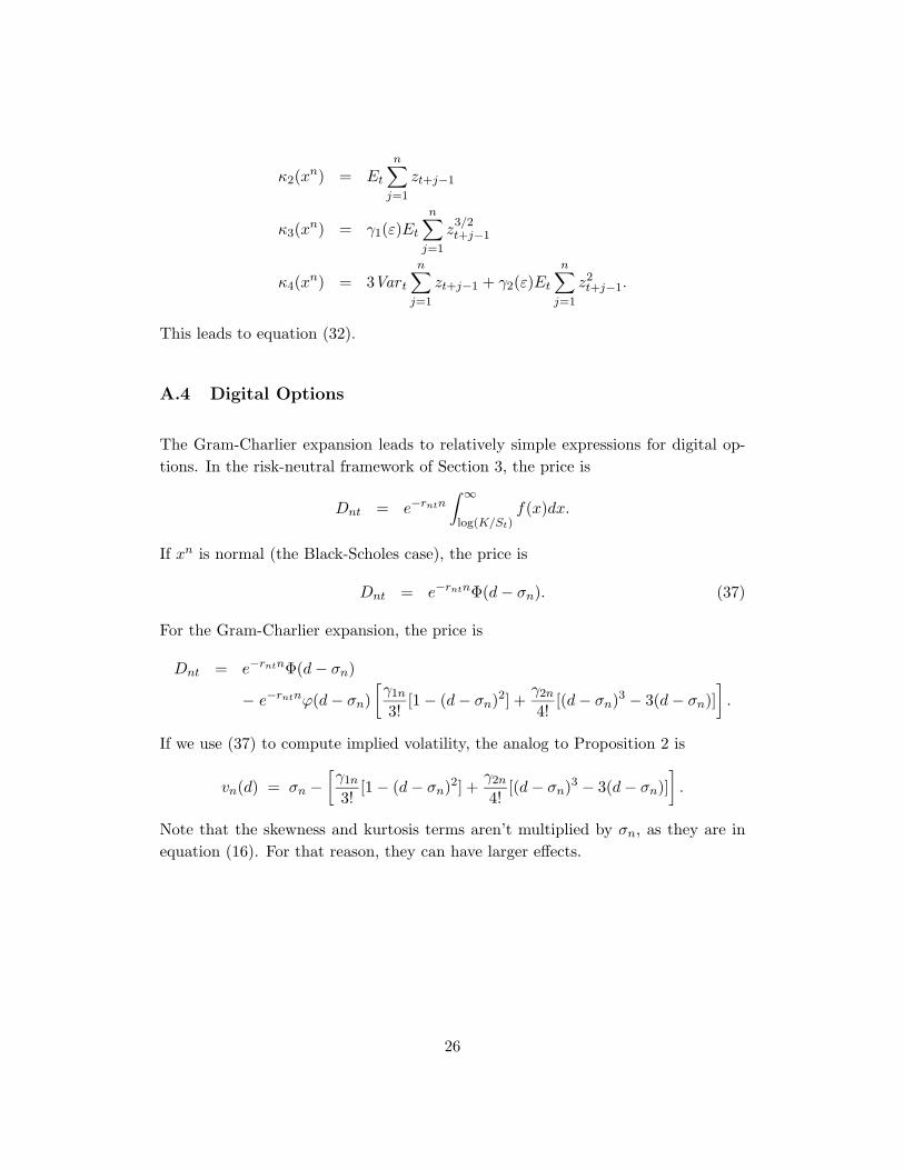
A.4 Digital Options

The Gram-Charlier expansion leads to relatively simple expressions for digital op-

tions. In the risk-neutral framework of Section 3, the price is

Dnt = e−rntn∫ ∞

log(K/St)f(x)dx.

If xn is normal (the Black-Scholes case), the price is

Dnt = e−rntnΦ(d− σn). (37)

For the Gram-Charlier expansion, the price is

Dnt = e−rntnΦ(d− σn)

− e−rntnϕ(d− σn)

[

γ1n

3![1 − (d− σn)2] +

γ2n

4![(d− σn)3 − 3(d− σn)]

]

.

If we use (37) to compute implied volatility, the analog to Proposition 2 is

vn(d) = σn −

[

γ1n

3![1 − (d− σn)2] +

γ2n

4![(d− σn)3 − 3(d− σn)]

]

.

Note that the skewness and kurtosis terms aren’t multiplied by σn, as they are in

equation (16). For that reason, they can have larger effects.

26

References

Abken, Peter, Dilip Madan, and Sailesh Ramamurtie, 1996, “Estimation of risk-

neutral and statistical densities by hermite polynomial approximation: With

an application to eurodollar futures options,” manuscript, Federal Reserve

Bank of Atlanta, June.

Ait-Sahalia, Yacine, and Andrew Lo, 1997, “Nonparametric estimation of state-

price densities implicit in financial asset prices,” manuscript, University of

Chicago, June.

Akgiray, Vedat, and Geoffrey Booth, 1988, “Mixed diffusion-jump process modeling

of exchange rate movements,” Review of Economics and Statistics 70, 631-

637.

Bakshi, Gurdip, Charles Cao, and Zhiwu Chen, 1997, “Empirical Performance of

Alternative Option Pricing Models,” Journal of Finance 52, 2002-2049.

Bakshi, Gurdip, Charles Cao, and Zhiwu Chen, 2000, “Pricing and Hedging Long-

Term Options,” Journal of Econometrics, 94(1-2), 277–318.

Bates, David, 1996a, “Jumps and stochastic volatility: Exchange rate processes

implicit in Deutsche mark options,” Review of Financial Studies 9, 69-107.

Bates, David, 1996b, “Dollar jump fears, 1984-1992: Distributional abnormalities

implicit in currency futures data,” Journal of International Money and Fi-

nance 15, 65-93.

Baillie, Richard, and Tim Bollerslev, 1989, “The message in daily exchange rates:

A conditional variance tale,” Journal of Business and Economic Statistics 7,

297-305.

Black, Fischer, and Myron Scholes, 1973, “The pricing of options and corporate

liabilities,” Journal of Political Economy 81, 637-654.

Black, Fischer, 1975, “Fact and fantasy in the use of options,” Financial Analysts

Journal 31 (July-August), 36-72.

Bodurtha, James, and Georges Courtadon, 1987, The Pricing of Foreign Currency

Options, Monograph Series in Finance and Economics 1987-4/5, New York:

Salomon Center.

27

Brenner, Menachem, and Young-Ho Eom, 1997, “No-arbitrage option pricing: New

evidence on the validity of the martingale property,” manuscript, New York

University and Federal Reserve Bank of New York.

Campa, Jose, and Kevin Chang, 1995, “Testing the expectations hypothesis on the

term structure of volatilities,” Journal of Finance 50, 529-547.

Campa, Jose, and Kevin Chang, 1996, “Arbitrage-based tests of target-zone credi-

bility: Evidence from ERM cross-rate options,” American Economic Review

86, 726-740.

Campa, Jose, Kevin Chang, and Robert Reider, 1997, “Implied exchange rate dis-

tributions: Evidence from OTC option markets,” manuscript, New York Uni-

versity, August.

Das, Sanjiv, and Rangarajan Sundaram, 1997, “Taming the skew: Higher-order

moments in modeling asset price processes in finance,” NBER Working Paper

No. 5976.

Diebold, Francis, 1988, Empirical Modeling of Exchange Rate Dynamics, New York:

Springer-Verlag.

Drost, Feike, and Theo Nijman, 1993, “Temporal aggregation of GARCH processes,”

Econometrica 61, 909-927.

Drost, Feike, Theo Nijman, and Bas Werker, 1996, “Estimation and testing in mod-

els containing both jumps and stochastic volatility,” forthcoming, Journal of

Business and Economic Statistics.

Garman, Mark, and Steven Kohlhagen, 1983, “Foreign currency option values,”

Journal of International Money and Finance 2, 231-237.

Hansen, Bruce, 1994, “Autoregressive conditional density estimation,” International

Economic Review 35, 705-730.

Hsieh, David, 1989, “Modeling heteroskedasticity in daily foreign exchange rates,”

Journal of Business and Economic Statistics 7, 307-317.

Jarrow, Robert, and Andrew Rudd, 1982, “Approximate option valuation for arbi-

trary stochastic processes,” Journal of Financial Economics 10, 347-369.

Johnson, Norman, Samuel Kotz, and N. Balakrishnan, 1994, Continuous Univariate

Distributions, Volume 1, Second Edition, New York: Wiley.

28

Jorion, Philippe, 1988, “On jump processes in the foreign exchange and stock mar-

kets,” Review of Financial Studies 1, 427-445.

Kim, Sangjoon, and Neil Shephard, 1994, “Stochastic volatility: Optimal likelihood

inference and comparison with ARCH models,” manuscript, Nuffield College,

Oxford, March.

Knight, John, and Stephen Satchell, 1997, “Pricing derivatives written on assets with

arbitrary skewness and kurtosis,” manuscript, Trinity College, Cambridge,

November.

Kochard, Larry, 1997, “Option pricing using higher order moments of the risk-

neutral probability density function,” manuscript, University of Virginia, De-

cember.

Kolassa, John, 1994, Series Approximation Methods in Statistics, New York: Springer-

Verlag.

Longstaff, Francis, 1995, “Option pricing and the martingale restriction,” Review of

Financial Studies 8, 1091-1124.

Madan, Dilip, and Frank Milne, 1994, “Contingent claims valued and hedged by

pricing and investing in a basis,” Mathematical Finance 4, 223-245.

Malz, Allan, 1996, “Option-based estimates of the probability distribution of ex-

change rates and currency excess returns,” manuscript, Federal Reserve Bank

of New York, March.

Melino, Angelo, and Stuart Turnbull, 1990, “Pricing foreign currency options with

stochastic volatility,” Journal of Econometrics 45, 239-265.

Merton, Robert, 1976, “Option pricing when underlying stock prices are discontin-

uous,” Journal of Financial Economics 3, 125-144.

Rosenberg, Joshua, 1996 “Pricing multivariate contingent claims using estimated

risk-neutral density functions,” manuscript, New York University, Novem-

ber.

Rubinstein, Mark, 1976, “The valuation of uncertain income streams and the pricing

of options,” Bell Journal of Economics 7, 407-425.

Taylor, Stephen, and Xinzhong Xu, 1994, “The magnitude of implied volatility

smiles: Theory and empirical evidence for exchange rates,” Review of Futures

Markets 13, 355-380.

Zhu, Yingzi, 1997, Three Essays in Mathematical Finance, Doctoral dissertation

submitted to the Department of Mathematics, New York University, May.

29

Table 1

Properties of Daily Exchange Rate Changes

Canadian German JapaneseStatistic Dollar Mark Yen

Mean (Annualized) 0.002 0.045 0.062Std Deviation (Annualized) 0.045 0.117 0.116Skewness –0.171 –0.090 0.351Kurtosis 3.558 2.204 6.936

Statistics pertain to daily depreciation rates, xt+1 = logSt+1−logSt, computed fromdollar prices S of other currencies. The data are from Datastream and cover businessdays between January 3, 1986 and May 16, 1996 (2704 observations). Means andstandard deviations have been multiplied by 260.6 and 260.61/2, respectively, toconvert them to annual units, where 260.6 is the average number of business daysin the years 1986-95. Skewness and (excess) kurtosis are the standard indicators;see equations (2,3).

30

Table 2

Properties of At-the-Money Volatilities

Canadian German Japanese BritishStatistic/Maturity Dollar Mark Yen Pound

Mean1 5.16 10.52 10.83 5.16242 5.22 10.72 11.18 5.21723 5.27 10.83 11.44 5.26686 5.41 11.00 11.84 5.411512 5.62 11.11 12.10 5.6209

Median1 5.05 9.90 9.98 5.052 5.30 10.24 10.83 5.303 5.55 10.50 11.30 5.556 5.80 11.00 12.07 5.8012 5.98 11.30 12.47 5.98

Standard Deviation1 1.64 2.94 3.21 1.642 1.50 2.62 2.88 1.503 1.40 2.39 2.68 1.406 1.17 2.05 2.31 1.1712 0.99 1.81 2.00 0.99

Autocorrelation1 0.948 0.984 0.978 0.9582 0.948 0.988 0.985 0.9483 0.943 0.991 0.988 0.9436 0.922 0.994 0.991 0.92212 0.894 0.995 0.993 0.894

Volatilities are quotes from a large international bank, expressed as annual per-centages, January 2, 1995, to January 6, 1997 (510 daily observations). See Zhu(1997).

31

Table 3

The Quality of Gram-Charlier Approximations

Maturity True Moments Proposition 1 Proposition 2

(month) σ γ1 γ2 σ γ1 γ2 σ γ1 γ2

A. Bakshi et al, SV modeln = 1 0.188–0.540 0.622 0.189 –0.623 0.582 0.186–0.642 0.472n = 3 0.189–0.845 1.324 0.198 –1.089 1.771 0.186–1.054 1.355n = 6 0.189–1.046 1.921 0.212 –1.465 3.062 0.184–1.261 2.043n = 12 0.189–1.197 2.395 0.234 –1.927 4.144 0.180–1.342 2.405

B. Bakshi et al, SVJ model

n = 1 0.154–0.799 1.586 0.158 –0.881 1.416 0.156–0.981 1.580n = 3 0.156–0.914 1.592 0.160 –1.031 1.636 0.154–1.018 1.713n = 6 0.156–0.957 1.738 0.162 –1.103 1.824 0.152–1.036 1.827n = 12 0.157–0.954 1.729 0.166 –1.130 1.847 0.150–0.970 1.586

C. Bates (1996), SV model

n = 1 0.155 0.027 0.399 0.155 0.028 0.281 0.155 0.036 0.281n = 3 0.155 0.026 0.803 0.155 0.027 0.670 0.155 0.062 0.646n = 6 0.155 0.006 1.176 0.155 0.010 1.000 0.155 0.086 0.948n = 12 0.155–0.033 1.444 0.154 –0.021 1.208 0.155 0.112 1.138

D. Bates (1996), SVJ model

n = 1 0.173 0.032 0.409 0.173 0.033 0.367 0.173 0.045 0.364n = 3 0.173 0.045 0.763 0.173 0.043 0.715 0.173 0.086 0.697n = 6 0.173 0.026 1.186 0.173 0.028 1.082 0.173 0.121 1.051n = 12 0.172–0.029 1.575 0.172 –0.010 1.388 0.172 0.160 1.339

Jump Stochastic Volatility

Parameters λ µj σj√

Vj α β σv ρ√

α/β

A. 0 0 0 0 0.04 1.15 0.39 –0.64 0.186B. 0.59 -0.05 0.07 0.0615 0.04 2.03 0.38 –0.57 0.140C. 0 0 0 0 0.0311.300.284 0.045 0.155D. 15.01 -0.0010.019 0.072 0.0190.780.343 0.078 0.144

The table reports implied conditional moments (volatility σ, skewness γ1 and kur-

32

tosis γ2) the jump-diffusion/stochastic volatility models estimated in Bates 91996)for currency options and in Bakshi, Cao, and Chen (1997) for stock options. Threemethods are used to obtain these moments: (1) numerical integration of the prob-ability density function (“true moments”), (2) Proposition 1, and (3) Proposition 2of this paper. The current spot price St is set to 100. Domestic and foreign interestrates are set to zero. For stochastic volatility model, the current volatility is set toequal its mean.

33

Table 4

Gram-Charlier Approximations to Jump-Diffusions

Parameters Estimates

Example σ0 σj σ γ1 γ2

A. Benchmark 0.0688 0.0230 0.1000 –0.006 0.898

B. Jump Intensity

Low (λ = 5) 0.0792 0.0273 0.0997 –0.005 0.748High (λ = 15) 0.0505 0.0193 0.1002 –0.007 1.046

C. Volatility

Low (σ = 0.05) 0.0344 0.0155 0.0500 –0.003 0.898High (σ = 0.2) 0.1375 0.0459 0.1999 –0.012 0.898

D. Maturity

Three Months 0.0295 0.0302 0.1004 –0.012 1.119Six Months (γ1 = 0.5) 0.0295 0.0302 0.1001 –0.009 0.540

E. Kurtosis

Low (γ2 = 0.5) 0.0792 0.0193 0.0999 –0.003 0.439High (γ2 = 1.5) 0.0595 0.0254 0.1001 –0.009 1.401

F. Skewness

Low (γ1 = −0.1) 0.0688 0.0229 0.0997 –0.006 0.897Medium (γ1 = −0.2) 0.0688 0.0227 0.0988 –0.006 0.897High (γ1 = −0.5) 0.0682 0.0206 0.0896 –0.004 0.801

The table reports parameters of jump-diffusion models (annualized standard devia-tions, σ0 and σj , of non-jump and jump components) and estimates of skewness andkurtosis (γ1 and γ2) implied by Gram-Charlier approximations to them based onequation (16). Errors in the approximation are indicated by differences between es-timates of skewness and kurtosis and their values in the corresponding jump model.For the benchmark case, γ1 = 0, γ2 = 1, annualized volatility σ = 0.1, annualizedjump intensity λ = 10, interest rates are zero, and the maturity of the option is onemonth. Exceptions are noted in the first column.

34

Table 5

Conditional Moments Implied by Volatility Smiles

Maturity Standard Deviation Skewness Kurtosis

Overnight 0.0849 –0.272 2.9121 Month 0.0892 –0.168 1.5912 Months 0.0973 –0.088 1.2183 Months 0.1018 –0.064 1.0336 Months 0.1087 –0.038 0.7529 Months 0.1111 –0.022 0.62112 Months 0.1116 0.002 0.54518 Months 0.1117 –0.006 0.447

Entries are moments inferred from the volatility smiles in Figure 9, as outlined inSection 4. The standard deviation σn is reported in annual units. Skewness andkurtosis are the standard indicators, γ1n and γ2n, defined in equations (2,3).

35

Figure 1

An Example of a Volatility Smile

−0.03 −0.02 −0.01 0 0.01 0.02 0.037.5

8

8.5

9

9.5

10

10.5

11

11.5

Log(S/K)

Impl

ied

Vol

atili

ty (P

erce

nt P

er Y

ear)

Overnight

1 Month

3 Months

6 Months

12 Months

The line plots implied volatility against moneyness for one-month over-the-counterDeutsche mark options on April 3, 1996. Moneyness d is defined by equation (9).

36

Figure 2

Median Implied Volatility by Maturity

0 2 4 6 8 10 120.6

0.65

0.7

0.75

0.8

0.85

0.9

0.95

1

Maturity in Months

Med

ian

Impl

ied

Vol

atili

ty (1

2−M

onth

=1)

Lines represent median implied volatility quotes for at-the-money options for theCanadian dollar (dotted line), German mark (dashed line), and Japanese yen (dash-dotted line). The lines are scaled to aid comparison: For each currency, medianvolatility has been divided by its value at 12 months.

37

Figure 3

Black-Scholes and Gram-Charlier Call Prices

−1.5 −1 −0.5 0 0.5 1 1.50

0.5

1

1.5

2

2.5

3

3.5

4

4.5

5

Moneyness d

Rat

io o

f Cal

l Pric

e to

Und

erly

ing

(Per

cent

)

Each line represents the relation between the call price and “moneyness” d for anunderlying distribution of log-changes in the spot exchange rate. The solid line is theBlack-Scholes formula, equation (8). The dashed and dash-dotted lines incorporate,respectively, skewness (γ1n = 2) and kurtosis (γ2n = 2) into the Gram-Charlier callprice formula, equation (15). In each case, we have set n = 260.6/12 (one month),σn = 0.10 ∗ (1/12)1/2 (0.10 annually), and rnt = r∗nt = 0.

38

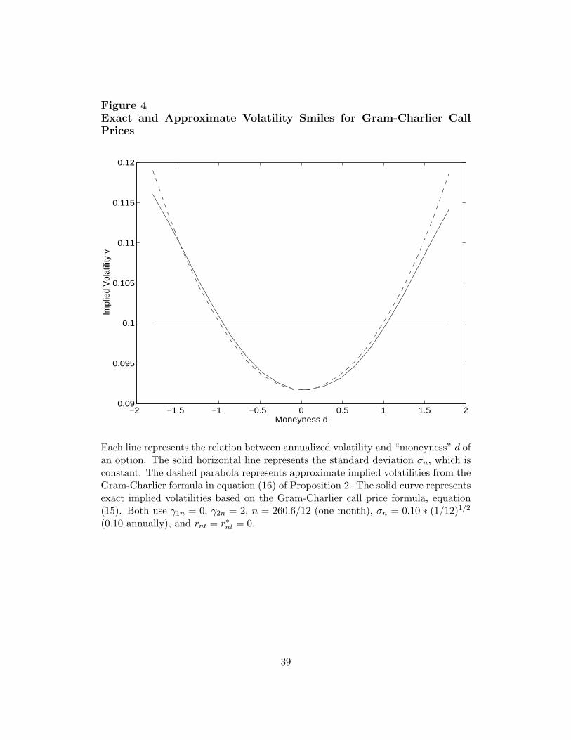
Figure 4

Exact and Approximate Volatility Smiles for Gram-Charlier Call

Prices

−2 −1.5 −1 −0.5 0 0.5 1 1.5 20.09

0.095

0.1

0.105

0.11

0.115

0.12

Moneyness d

Impl

ied

Vol

atili

ty v

Each line represents the relation between annualized volatility and “moneyness” d ofan option. The solid horizontal line represents the standard deviation σn, which isconstant. The dashed parabola represents approximate implied volatilities from theGram-Charlier formula in equation (16) of Proposition 2. The solid curve representsexact implied volatilities based on the Gram-Charlier call price formula, equation(15). Both use γ1n = 0, γ2n = 2, n = 260.6/12 (one month), σn = 0.10 ∗ (1/12)1/2

(0.10 annually), and rnt = r∗nt = 0.

39

Figure 5

Effects of Skewness and Kurtosis on Gram-Charlier Call Prices

−1.5 −1 −0.5 0 0.5 1 1.50.09

0.095

0.1

0.105

0.11

0.115

0.12

Moneyness d

Impl

ied

Vol

atili

ty v

The lines graph approximate annualized implied volatility against moneyness d fordifferent values of higher moments in the distribution of log-changes in the spotexchange rate. The horizontal solid line represents Black-Scholes. The smile (curvedsolid line) has positive kurtosis but no skewness (γ1n = 0, γ2n = 2). The skew(dashed line) has negative skewness and positive kurtosis (γ1n = −0.4, γ2n = 0.5).Both are based on the approximation (16). In each case, n = 260.6/12 (one month),σn = 0.10 ∗ (1/12)1/2 (0.10 annually), and rnt = r∗nt = 0.

40

Figure 6

Deltas for Black-Scholes and Gram-Charlier Call Prices

−2 −1.5 −1 −0.5 0 0.5 1 1.5 20

0.1

0.2

0.3

0.4

0.5

0.6

0.7

0.8

0.9

1

Moneyness d

Del

ta

Each line represents the relation between the ∆ and “moneyness” d for an underlyingdistribution of log-changes in the spot exchange rate. The solid line is Black-Scholes:∆(d) = Φ(d). The dashed and dash-dotted lines incorporate, respectively, skewness(γ1n = 2) and kurtosis (γ2n = 2) into the Gram-Charlier ∆, equation (17). Otherparameter values are the same as Figure 4.

41

Figure 7

Gram-Charlier Volatility Smiles for Two Maturities

−1.5 −1 −0.5 0 0.5 1 1.50.09

0.095

0.1

0.105

0.11

0.115

0.12

Moneyness d

Impl

ied

Vol

atili

ty v

The lines represent volatility smiles for two different maturities. The horizontalsolid line represents Black-Scholes. The curved lines have positive kurtosis (γ2n =2 × 260.6/(12n)) for n = 260.6/12 (one month, solid line) and n = 3 × 260.6/12(three months, dashed line). Both are based on the approximation (16). Otherparameters are σn = 0.10 ∗ (1/12)1/2 (0.10 annually), and rnt = r∗nt = 0.

42

Figure 8

Kurtosis in Currency Prices Over Different Time Horizons

0 5 10 15 20 25 30 35 40 45 50−0.2

0

0.2

0.4

0.6

0.8

1

Time Interval n in Days

Kurto

sis

Rel

ativ

e to

n=1

Lines represent estimates of kurtosis (γ2n) for time intervals of n days relative ton = 1. The solid line is 1/n and serves as a theoretical benchmark. The other linesare estimates for the Canadian dollar (dotted line), German mark (dashed line), andJapanese yen (dash-dotted line), all for the same time period covered by Table 1.

43

Figure 9

Volatility Smiles for Deutsche mark Options on April 3, 1996

−1.5 −1 −0.5 0 0.5 1 1.57.5

8

8.5

9

9.5

10

10.5

11

11.5

Moneyness d

Impl

ied

Vol

atili

ty (P

erce

nt P

er Y

ear)

Overnight

1 Month

3 Months

6 Months

12 Months

Lines describe volatility smiles for over-the-counter Deutsche mark options on April3, 1996. The maturities of the options are noted in the figure.

44

Figure 10

Conditional Kurtosis with Stochastic Volatility

0 2 4 6 8 10 12 14 16 180

0.5

1

1.5

2

2.5

3

Maturity in Months

Con

ditio

nal K

urto

sis

The figure describes conditional kurtosis v. maturity in the data and in the stochas-tic volatility model of Section 7. Asterisks represent the data: the values of im-plied kurtosis reported in Table 4. The solid line is the stochastic volatility modelwith non-normal innovations. The dashed line represents the same model withoutstochastic volatility: α = 0 (essentially a pure jump model). The dash-dotted linerepresents the model with normal innovations: γ2(ε) = 0 (a gaussian stochasticvolatility model).

45