Accounting for Trade Patterns∗

Stephen J. ReddingPrinceton University, NBER and CEPR †

David E. WeinsteinColumbia University and NBER‡

March 7, 2018

Abstract

We develop a quantitative framework for exactly decomposing trade patterns into economically mean-ingful components. We derive price indexes that determine comparative advantage across countries andsectors and the aggregate cost of living. If rms and products are imperfect substitutes, we show that theseprice indexes depend on variety, average demand or quality, and the dispersion of demand or quality-adjusted prices, and are only weakly related to standard empirical measures of average prices, therebyproviding insight for elasticity puzzles. Of the cross-section (time-series) variation in comparative ad-vantage, 50 (90) percent is accounted for by variety and average demand or quality, with average pricescontributing less than 10 percent.

JEL CLASSIFICATION: F11, F12, F14KEYWORDS: comparative advantage, trade, prices, quality, variety

∗We are especially grateful to Rob Feenstra, Keith Head, Pete Klenow, Kalina Manova, Thierry Mayer, Marc Melitz, GianmarcoOttaviano and Daniel Xu for helpful comments. We would also like to thank colleagues and seminar participants at Carnegie-Mellon, Chicago, Columbia, Duke, NBER, Princeton, Stanford and UC Berkeley for helpful comments. Thanks to Mark Greenan,Ildiko Magyari, Charly Porcher and Dyanne Vaught for outstanding research assistance. Redding and Weinstein thank Princetonand Columbia respectively for research support. Weinstein would also like to thank the NSF (Award 1127493) for generous nancialsupport. Any opinions, ndings, and conclusions or recommendations expressed in this paper are those of the authors and do notnecessarily reect the views of the U.S. Census Bureau or any organization to which the authors are aliated. Results have beenscreened to insure that no condential data are revealed.

†Fisher Hall, Princeton, NJ 08544. Email: reddings@princeton.edu.‡420 W. 118th Street, MC 3308, New York, NY 10027. Email: dew35@columbia.edu.

1

1 Introduction

International economists face a large number of modeling choices when constructing models aimed at match-ing international trade ows and welfare gains. In particular, it is not always obvious how to model the impactof international cost, quality, entry, and demand dierences on trade volumes. Moreover, even if one did knowthe correct supply-side model, ocial price indexes are often constructed using very dierent formulas thanthose implied by the constant elasticity of substitution (CES) demand systems that dominate trade and macro.Thus, models may perform poorly because objects like import price indexes are dened by statistical agenciesin very dierent ways than the theoretical objects in economic models.

This paper makes three contributions to our understanding of trade ows and aggregate welfare gains.First, we show how to use commonly available trade-transactions data to rigorously measure aggregate andimport price indexes even when data (such as the prices of domestically produced tradables and non-tradables)are incomplete or missing. Second, we develop a method for exactly decomposing aggregate trade ows andrevealed comparative advantage (RCA) into four factors that vary both in the cross section and the timeseries: average prices, the entry and exit of products and rms, demand or quality shifts, and the dispersionor heterogeneity of rm and product sales. Each of these factors has been emphasized in some form in manyempirical implementations of trade models (c.f., (Crozet, Head, and Mayer 2012; Hallak and Schott (2011);Kehoe and Ruhl 2013; Manova and Zhang (2012); Mayer, Melitz, and Ottaviano 2014), but a key feature of oursetup is that we can allow all of them to matter without needing to make any assumptions about the supply-side of the model. Finally, we develop novel moments for price and sales distributions that are necessary forany model to match trade patterns and import price changes in a CES demand system.

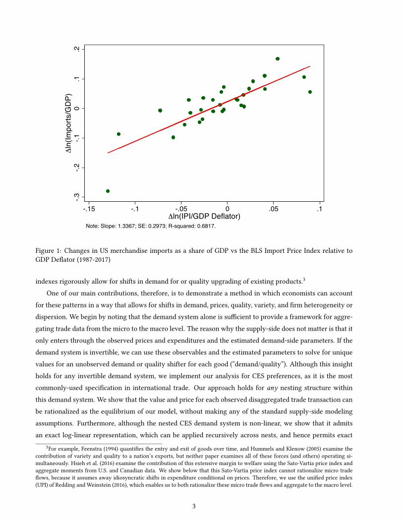
One can understand the challenge of linking import prices and import volumes by considering one of theearliest stylized facts in international economics: aggregate import prices and import volumes have correla-tions that are often the wrong sign or close to zero (c.f., Adler 1945).1 Figure 1 shows the relationship for theU.S. between the change in log of merchandise imports divided by GDP and the log in the change in the ImportPrice Index divided by the the GDP deator over the last 30 years.2 The slope of the line is 1.3, which, if weinterpret through the lens of a CES demand system in the absence demand shifts, would imply that the importdemand curve slopes upwards. Since Orcutt (1950), economists have long known the two main explanationsfor the relationship we see in Figure 1: “shifts of the demand schedule” and “faulty methods of [price] indexconstruction.” Demand shifts are typically ruled out a priori in almost all trade and macro models (which arebased on time-invariant utility functions), and hence their ability to match actual ows requires us to believein Orcutt’s second explanation: that our price indexes are faulty and do not properly adjust for quality, va-riety, and other factors. However, this implies that even if we knew the relationship between imports andtheoretically-correct price indexes, ocial price indexes do not capture important factors driving imports.Although Feenstra (1994) showed how to build price indexes that capture changes in variety, no import price

1For example, Adler writes, “While real income may account for most of the variation in imports, the remaining variation doesnot seem to be explained by changes in relative prices.”

2We chose this particular specication because it can be motivated by a CES demand system. The lack of a clear negativerelationship is not something that can be solved by simply changing the specication to long dierences, levels, or just using realimports on the vertical axis.

2

-.3-.2

-.10

.1.2

Δln

(Impo

rts/G

DP)

-.15 -.1 -.05 0 .05 .1Δln(IPI/GDP Deflator)

Note: Slope: 1.3367; SE: 0.2973; R-squared: 0.6817.

Figure 1: Changes in US merchandise imports as a share of GDP vs the BLS Import Price Index relative toGDP Deator (1987-2017)

indexes rigorously allow for shifts in demand for or quality upgrading of existing products.3

One of our main contributions, therefore, is to demonstrate a method in which economists can accountfor these patterns in a way that allows for shifts in demand, prices, quality, variety, and rm heterogeneity ordispersion. We begin by noting that the demand system alone is sucient to provide a framework for aggre-gating trade data from the micro to the macro level. The reason why the supply-side does not matter is that itonly enters through the observed prices and expenditures and the estimated demand-side parameters. If thedemand system is invertible, we can use these observables and the estimated parameters to solve for uniquevalues for an unobserved demand or quality shifter for each good (“demand/quality”). Although this insightholds for any invertible demand system, we implement our analysis for CES preferences, as it is the mostcommonly-used specication in international trade. Our approach holds for any nesting structure withinthis demand system. We show that the value and price for each observed disaggregated trade transaction canbe rationalized as the equilibrium of our model, without making any of the standard supply-side modelingassumptions. Furthermore, although the nested CES demand system is non-linear, we show that it admitsan exact log-linear representation, which can be applied recursively across nests, and hence permits exact

3For example, Feenstra (1994) quanties the entry and exit of goods over time, and Hummels and Klenow (2005) examine thecontribution of variety and quality to a nation’s exports, but neither paper examines all of these forces (and others) operating si-multaneously. Hsieh et al. (2016) examine the contribution of this extensive margin to welfare using the Sato-Vartia price index andaggregate moments from U.S. and Canadian data. We show below that this Sato-Vartia price index cannot rationalize micro tradeows, because it assumes away idiosyncratic shifts in expenditure conditional on prices. Therefore, we use the unied price index(UPI) of Redding and Weinstein (2016), which enables us to both rationalize these micro trade ows and aggregate to the macro level.

3

additive decompositions of aggregate variables.Our rst main contribution is to use this trade nesting structure to derive exact aggregate price indexes at

the national and exporter-sector level that are separable into average price, demand/quality, variety, and rmdispersion terms. The average price term has a functional form that corresponds closely to a conventionalprice index like the BLS import price index. The demand/quality term corrects the price index for shifts in animporter’s demand for another country’s exports, either due to a change of tastes for the exporter’s outputor quality upgrading of existing goods by exporters. The variety term captures how changes in the numberof products in each rm and in the number of rms aect exports, and the dispersion term captures howchanges in the size distribution of rms (e.g. as determined by demand and productivity dierences acrossrms) aect exports when goods are imperfect substitutes. In addition, we also show how to aggregate tothe national level even when detailed price and quantity data for certain sectors (e.g. non-traded sectors) isincomplete or missing.

Unlike prior import price indexes, our indexes allow not only for changes in prices and variety, but alsodemand and quality of existing goods. Thus, unlike frameworks built on time-invariant utility functions, itis possible in our setup that patterns like the one in Figure 1 can be driven by demand shifts. Importantly,we provide a quantication of each of the factors that are omitted when only prices are used to constructmeasures of import prices. Thus, while we show that the average price term has a similar functional formand turns out to be highly correlated with the BLS import price index (ρ = 0.72), the other terms in our priceindex have very dierent functional forms and turn out to be are negatively correlated with the BLS importprice index. The importance of these terms helps explain the diculty of trying to understand trade patternsusing only conventional measures of import and domestic prices.

Our next theoretical contribution is to develop a rigorous measure of revealed comparative advantage(RCA) that is valid for the CES demand system and depends on the relative values of our price index acrosscountries and sectors. This RCA measure is also additively separable into price, demand/quality, entry/exit,and dispersion terms in both the cross-section and time series. This property enables us to seamlessly movebetween the contribution of each factor to price indexes and how they aect import volumes. Thus, forexample, when we observe that Chinese exports to the US rose dramatically between 1998 and 2011 in spiteof a relative increase in Chinese export prices, we can do more than just note the factors that are left outof conventional indexes—our method enables us to exactly decompose this rise in Chinese imports into theamount attributable to each factor.

Our last theoretical contribution is to derive a general expression for understanding when distributionalassumptions will and will not matter for understanding movements in import prices and trade patterns. Therehave been a number of proposed distributions for modeling the underlying rm productivity distributionsthat give rise to observed trade patterns: Pareto, Fréchet, and log normal being the most prominent ones.These distributional assumptions are made for reasons of tractability in theoretical models of internationaltrade. However, it is less clear how much the assumed distributional assumptions matter for interpretingthe results. Our paper makes both a destructive and a constructive contribution. On the negative side, weshow that detailed trade-transactions data formally reject all three of these distributions, which means that

4

although models based on these specications may t the aggregate data, they do not fully capture what ishappening at the micro level. However, we also demonstrate an irrelevance result. In a CES setup, it does notmatter what the underlying productivity distribution is for understanding trade patterns and import pricesas long as the distribution is correctly centered such that it matches the geometric average price, geometricaverage quality, and geometric average sales of each rm. Thus, calibrated models will correctly capturetrade ows and import price changes if their choice of distributional parameters enables them match thesegeometric averages in the data. For example, we show that parameters satisfying these criteria can easilybe recovered from the QQ-estimation framework introduced into the trade literature by Head, Mayer, andThoenig (2016).

We implement our approach using both U.S. data from 1997-2011 (reported in the main paper) and alsoChilean data from 2007-14 (reported in the web appendix). Our decomposition reveals that rm entry/exitand average demand/quality each account for around 45 percent of the time-series variation in imports, withthe dispersion of demand-adjusted prices making up most of the rest. We demonstrate that this pattern isrobust across a range of alternative values for the elasticities of substitution. Indeed, for parameter values forwhich goods are imperfect substitutes, we show that the contributions from rm entry/exit and the disper-sion of demand-adjusted prices to patterns of trade are invariant to these assumed elasticities. The fact thatthe prices of continuing goods are not negatively associated with the time-series variation in imports (as wesaw in Figure 1) does not mean that prices do not matter for import volumes. Indeed, we estimate steeplynegative demand curves. However, the data suggest that equilibrium price increases are small and associatedwith rm entry and demand/quality shifts that often more than oset whatever impact the price movementhas. Similarly, in the cross-section, prices matter little in equilibrium with rm variety and dispersion (het-erogeneity) accounting for close to 70 percent of the variation in trade patterns. In sum, these results suggestthat models that emphasize small equilibrium movements in average prices and larger movements in otherfactors are more likely to capture the underlying forces at work.

Although there is an exact mapping between our price index and observed trade ows, the same need notbe true for other approaches that impose stronger assumptions, such as the Feenstra (1994) price index, whichcorresponds to a special case in which there are no demand shifts for surviving goods. Thus, the dierencebetween observed trade patterns and those predicted using alternative price indexes provides a metric forhow successful models based on these assumptions are. By comparing actual RCA with counterfactual valuesof RCA based on dierent assumptions—e.g., with or without demand-shifts or variety corrections—we candirectly assess the implications of these simplifying assumptions for understanding trade patterns. In particu-lar, we nd that models that assume no demand shifts and no changes in variety perform poorly on trade data.Models that incorporate variety changes while maintaining the assumption of no demand shifts do better, butstill can only account for about ten percent of the changes in comparative advantage over time. These nd-ings highlight the importance of changes in demand/quality within surviving varieties in understanding thechanges in comparative advantage documented in Freund and Pierola (2015) and Hanson, Lind and Muendler(2015). They also point to the relevance of dynamic trade theories, in which comparative advantage evolvesendogenously with process and product innovation, as in Grossman and Helpman (1991).

5

Our paper is related to several strands of existing research. First, we build on a long tradition in interna-tional trade that examines how to develop measures of prices in which quality and/or variety are changing(Feenstra 1994, Hallak and Schott 2011, and Feenstra and Romalis 2014). The papers developed important in-sights into how to adjust prices for variety and quality. However, none of them provide a method for exactlydecomposing trade ows into the various factors explained by these forces. Our decomposition also builds onHottman, Redding, and Weinstein (2016), which provides a methodology for doing a similar decompositionwithin consumer sectors using bar-code data. This paper extends that method to show how to aggregateacross sectors even when some of the sectoral price data is missing. Thus, while Hottman et al found thatwithin-rm demand/quality and product scope accounted for the vast majority of variation in sales acrossrms within sectors, they do not discuss variation across sectors or even aggregate variation in sales. Indeed,the two key factors that account for most of the variation in trade patterns—rm variety and rm disper-sion—do not even appear in their earlier work. We also make use of the price index developed Redding andWeinstein (2016) but modify it by adding a nesting structure that not allows for rms, multiple sectors, andmissing price data. These additions change both how the price indexes are constructed and how the param-eters are estimated. Moreover, Redding and Weinstein (2016) do not consider how to use these indexes toconstruct aggregate real output measures.

Second, research has relaxed the constant-elasticity assumptions in neoclassical trade models by providingconditions under which they reduce to exchange models in which countries directly trade factor services (seeAdao, Costinot and Donaldson 2017). In contrast, we assume a constant elasticity of demand, but relax theassumption of a constant elasticity of supply. By using additional structure on the demand-side, we are ableto rationalize both micro and macro trade data, enabling us to aggregate up from the micro level and quantifythe importance of dierent micro mechanisms for macro variables. As a result of imposing less structureon the supply-side, we can encompass non-neoclassical models with imperfect competition and increasingreturns to scale (including Krugman 1980, Melitz 2003, and Atkeson and Burstein 2008).

Finally, our paper is related to the literature estimating elasticities of substitution between varieties andquantifying the contribution of new goods to welfare. As shown in Feenstra (1994), the contribution of en-try and exit to the change in the CES price index can be captured using the expenditure share on commonproducts (supplied in both periods) and the elasticity of substitution. Building on this approach, Broda andWeinstein (2006) quantify the contribution of international trade to welfare through an expansion on the num-ber of varieties, and Broda and Weinstein (2010) examine product creation and destruction over the businesscycle. Other related research using scanner data to quantify the eects of globalization includes Handbury(2013), Atkin and Donaldson (2015), and Atkin, Faber, and Gonzalez-Navarro (2015), and Fally and Faber(2016). Whereas this existing research assumes that demand/quality is constant for each surviving variety,we show that allowing for time-varying demand/quality is central to both rationalizing both aggregate anddisaggregate patterns of trade.

The remainder of the paper is structured as follows. Section 2 introduces our theoretical framework.Section 3 outlines our structural estimation approach. Section 4 discusses our data. Section 5 reports ourempirical results. Section 6 concludes. A web appendix contains technical derivations, additional empirical

6

results for the U.S., and a replication of our U.S. results using Chilean data.

2 Theoretical Framework

We begin by showing that our framework exactly rationalizes observed micro trade data and permits exactaggregation, so that it can be used to quantify the importance of dierent micro mechanisms for macrovariables. Although our approach could be implemented for any nested demand system that is invertible,we focus on CES preferences as the leading demand system in international trade, with a nesting structureguided by existing theories of trade, which distinguish countries, sectors, rms and products.

Throughout the paper, we index importing countries (“importers”) by j and exporting countries (“ex-porters”) by i (where each country can buy its own output). Each exporter can supply goods to each importerin a number of sectors that we index by g (a mnemonic for “group”). We denote the set of sectors by ΩG andwe indicate the number of elements in this set by NG. We denote the set of countries from which importer j

sources goods in sector g at time t by ΩIjgt and we indicate the number of elements in this set by N I

jgt. Eachsector (g) in each exporter (i) is comprised of rms, indexed by f (a mnemonic for “rm”). We denote the setof rms in sector g that export from country i to country j at time t by ΩF

jigt; and we indicate the numberof elements in this set by NF

jigt. Each active rm can supply one or more products that we index by u (amnemonic for “unit,” as our most disaggregated unit of analysis); we denote the set of products supplied byrm f at time t by ΩU

f t; and we indicate the number of elements in this set by NUf t.

4

2.1 Demand

The aggregate unit expenditure function for importer j at time t (Pjt) is dened over the sectoral price index(PG

jgt) and “demand”5 parameter (ϕGjgt) for each sector g ∈ ΩG:

Pjt =

∑g∈ΩG

(PG

jgt/ϕGjgt

)1−σG

11−σG

, σG > 1, ϕGjgt > 0, (1)

where σG is the elasticity of substitution across sectors and ϕGjgt captures the relative demand for each sector.

The unit expenditure function for each sector g depends on the price index (PFf t) and demand parameter (ϕF

f t)for each rm f ∈ ΩF

jigt from each exporter i ∈ ΩIjgt within that sector:

PGjgt =

∑i∈ΩI

jgt

∑f∈ΩF

jigt

(PF

f t/ϕFf t

)1−σFg

11−σF

g

, σFg > 1, ϕF

f t > 0, (2)

4We use the superscript G to denote a sector-level variable, the superscript F to represent a rm-level variable, and the superscriptU to indicate a product-level variable. We use subscripts j and i to index individual countries, the subscript g to reference individualsectors, the subscript f to refer to individual rms, the subscript u to label individual products, and the subscript t to indicate time.

5There is no standard way to refer to this parameter. It is “taste” in Feenstra (1994), “quality” in Broda and Weinstein (2010), and“appeal” in Hottman, Redding and Weinstein (2016). We will refer to this parameter as either “demand” or “demand/quality” becauseit is isomorphic in the CES setup to have consumers demand more of a good conditional on price because it is higher quality in someobjective sense or because they just like it more. We therefore refer to the parameter as “demand” or “demand/quality” because itcorresponds to anything that shifts consumer demand conditional on price.

7

where σFg is the elasticity of substitution across rms f for sector g and ϕF

f t controls the relative demandfor each rm within that sector. We assume that the unit expenditure function within each sector takes thesame form for both nal consumption and intermediate use, so that we can aggregate both these sources ofexpenditure, as in Eaton and Kortum (2002) and Caliendo and Parro (2015).

We allow rm varieties to be horizontally dierentiated and assume the same elasticity of substitutionfor domestic and foreign rms within sectors (σF

g ).6 The unit expenditure function for each rm f dependson the price (PU

ut) and demand parameter (ϕUut) for each product u ∈ ΩU

f t supplied by that rm:

PFf t =

∑u∈ΩU

f t

(PU

ut/ϕUut

)1−σUg

11−σU

g

, σUg > 1, ϕU

ut > 0, (3)

where σUg is the elasticity of substitution across products within rms for sector g and ϕU

ut captures the relativedemand for each product within a given rm.

A few remarks about this specication are useful. First, we allow prices to vary across products, rms,sectors and countries, which implies that our setup nests models in which relative and absolute productioncosts dier within and across countries. Second, for notational convenience, we dene the rm index f ∈ΩF

jigt by sector g, destination country j and source country i. Therefore, if a rm has operations in multiplesectors and/or exporting countries, we label these dierent divisions separately. As we observe the prices ofthe products for each rm, sector and exporting country in the data, we do not need to take a stand on marketstructure or the level at which product introduction and pricing decisions are made within the rm. Third,the fact that the elasticities of substitution across products within rms (σU

g ), across rms within sectors(σF

g ), and across sectors within countries (σG) need not be innite implies that our framework nests modelsin which products are dierentiated within rms, across rms within sectors, and across sectors. Moreover,our work is robust to collapsing one or more of these nests. For example, if all three elasticities are equal(σU

g = σFg = σG), all three nests collapse, and the model becomes equivalent to one in which consumers only

care about rm varieties. Alternatively, if σUg = σF

g = ∞ and σG < ∞, only sectors are dierentiated, andvarieties are perfectly substitutable within sectors. Finally, if σU

g = σFg > σG, rm brands are irrelevant, so

that products are equally dierentiated within and across rms for a given sector.Fourth, the demand shifters (ϕG

jgt, ϕFf t, ϕU

ut) capture anything that shifts the demand for sectors, rms andproducts conditional on price. Therefore, they incorporate both quality (vertical dierences across varieties)and consumer tastes. We refer to these demand shifters as “demand/quality” to make clear that they can beinterpreted either as shifts in consumer demand or product quality.7 Finally, in order to simplify notation,we suppress the subscript for importer j, exporter i, and sector g for the rm and product demand shifters

6Therefore, we associate horizontal dierentiation within sectors with rm brands, which implies that dierentiation acrosscountries emerges solely because there are dierent rms in dierent countries, as in Krugman (1980) and Melitz (2003). It is straight-forward to also allow the elasticity of substitution to dier between home and foreign rms, which introduces separate dierentiationby country, as in Armington (1969). Feenstra, Luck, Obstfeld and Russ (2014) nd that they often cannot reject the same elasticitybetween home and foreign varieties as between foreign varieties.

7See, for example, the discussion in Di Comite, Thisse and Vandenbussche (2014). A large literature in international trade hasinterpreted these demand shifters as capturing product quality, including Schott (2004), Khandelwal (2010), Hallak and Schott (2011),Feenstra and Romalis (2008), and Sutton and Treer (2016).

8

(ϕFf t, ϕU

ut). However, we take it as understood that we allow these demand shifters for a given rm f andproduct u to vary across importers j, exporters i and sectors g, which captures the idea that a rm’s varietiescan be more appealing in some markets than others. For example, Sony products may be more appealing toAmericans than Chileans, or may have more consumer appeal in the television sector than the camera sector,or even may be perceived to have higher quality if they are supplied from Japan rather than from anotherlocation.

2.2 Non-traded Sectors

We allow some sectors to be non-traded, in which case we do not observe products within these sectorsin our disaggregated import transactions data, but we can measure total expenditure on these non-tradedsectors using domestic expenditure data. We incorporate these non-traded sectors by re-writing the overallunit expenditure function in equation (1) in terms of the share of expenditure on tradable sectors (µT

jt) and aunit expenditure function for these tradable sectors (PT

jt):

Pjt =(

µTjt

) 1σG−1

PTjt. (4)

The share of expenditure on the set of tradable sectors ΩT ⊆ ΩG (µTjt) can be measured using aggregate data

on expenditure in each sector:

µTjt ≡

∑g∈ΩT XGjgt

∑g∈ΩG XGjgt

=∑g∈ΩT

(PG

jgt/ϕGjgt

)1−σG

∑g∈ΩG

(PG

jgt/ϕGjgt

)1−σG , (5)

where XGjgt is total expenditure by importer j on sector g at time t. The unit expenditure function for tradable

sectors (PTjt) depends on the price index for each tradable sector (PG

jgt):

PTjt ≡

∑g∈ΩT

(PG

jgt/ϕGjgt

)1−σG

11−σG

, (6)

where we use the “blackboard” font P to denote price indexes that are dened over tradable goods.Therefore, our assumption on demand allows us to construct an overall price index without observing

entry, exit, sales, prices or quantities of individual products in non-tradable sectors. From equation (5), thereis always a one-to-one mapping between the market share of tradable sectors and the relative price indexesin the two sets of sectors. In particular, if the price of non-tradables relative to tradables rises, the share oftradables (µT

jt) also rises. In other words, the share of tradables is a sucient statistic for understanding therelative prices of tradables and non-tradables. As one can see from equation (4), if we hold xed the price oftradables (PT

jt), a rise in the share of tradables (µTjt) can only occur if the price of non-tradables sectors also

rises, which means that the aggregate price index index (Pjt) must also be increasing in the share of tradables.

2.3 Domestic Versus Foreign Varieties Within Tradable Sectors

We also allow for domestic varieties within tradable sectors, in which case we again do not observe themin our import transactions data, but we can back out the implied expenditure on these domestic varieties

9

using data on domestic shipments, exports and imports for each tradable sector. We incorporate domesticvarieties within tradable sectors by re-writing the sectoral price index in equation (2) in terms of the shareof expenditure on foreign varieties within each sector (the sectoral import share µG

jgt) and a unit expenditurefunction for these foreign varieties (a sectoral import price index PG

jgt):

PGjgt =

(µG

jgt

) 1σF

g −1 PGjgt. (7)

The sectoral import share (µGjgt) equals total expenditure on imported varieties within a sector divided by total

expenditure on that sector:

µGjgt ≡

∑i∈ΩEjgt

∑ f∈ΩFjigt

XFf t

XGjgt

=∑i∈ΩE

jgt∑ f∈ΩF

jigt

(PF

f t/ϕFf t

)1−σFg

∑i∈ΩIjgt

∑ f∈ΩFjigt

(PF

f t/ϕFf t

)1−σFg

, (8)

where ΩEjgt ≡

ΩI

jgt : i 6= j

is the subset of foreign countries i 6= j that supply importer j within sector g

at time t; XFf t is expenditure on rm f ; and XG

jgt is country j’s total expenditure on all rms in sector g attime t. The sectoral import price index (PG

jgt) is dened over the foreign goods observed in our disaggregatedimport transactions data as:

PGjgt ≡

∑i∈ΩE

jgt

∑f∈ΩF

jigt

(PF

f t/ϕFf t

)1−σFg

11−σF

g

. (9)

In this case, the import share within each sector is the appropriate summary statistic for understandingthe relative prices of home and foreign varieties within that sector. From equation (7), the sectoral price index(PG

jgt) is increasing in the sectoral foreign expenditure share (µGjgt). The reason is that our expression for the

sectoral price index (PGjgt) conditions on the price of foreign varieties, as is captured by the import price index

(PGjgt). For a given value of this import price index, a higher foreign expenditure share (µG

jgt) implies thatdomestic varieties are less attractive, which implies a higher sectoral price index.8

2.4 Exporter Price Indexes

To examine the contribution of individual countries to trade patterns and aggregate prices, it proves conve-nient to rewrite the sectoral import price index (PG

jgt) in equation (9) in terms of price indexes for each foreignexporting country within that sector (PE

jigt):

PGjgt =

∑i∈ΩE

jgt

(PE

jigt

)1−σFg

11−σF

g

, (10)

8In contrast, the expression for the price index in Arkolakis, Costinot and Rodriguez-Clare (2012) conditions on the price ofdomestically-produced varieties, and is increasing in the domestic expenditure share. The intuition is analogous. For a given priceof domestically-produced varieties, a higher domestic trade share implies that foreign varieties are less attractive, which implies ahigher price index.

10

where importer j’s price index for exporter i in sector g at time t (PEjigt) is dened over the rm price indexes

(PFf t) and demand/qualities (ϕF

f t) for each of the rms f from that foreign exporter and sector:

PEjigt ≡

∑f∈ΩF

jigt

(PF

f t/ϕFf t

)1−σFg

11−σF

g

, (11)

and we use the superscript E to denote a variable for a foreign exporting country.This exporter price index (11) is a key object in our empirical analysis, because it summarizes importer j’s

cost of sourcing goods from exporter i within sector g at time t. We show below that the relative values of theseexporter price indexes across countries and sectors determine comparative advantage. Note that substitutingthis denition of the exporter price index (11) into the sectoral import price index (10), we recover our earlierequivalent expression for the sectoral import price index in equation (9).

2.5 Expenditure Shares

Using the properties of CES demand, the share of each product in expenditure on each rm (SUut) is given by:

SUut =

(PU

ut/ϕUut)1−σU

g

∑`∈ΩUf t

(PU`t /ϕU

`t

)1−σUg

, (12)

where the rm and sector expenditure shares are dened analogously.In the data, we observe product expenditures (XU

ut) and quantities (QUut) for each product category. In

our baseline specication in the paper, we assume that the level of disaggregation at which products areobserved in the data corresponds to the level at which rms make product decisions. Therefore, we measureprices using unit values (PU

ut = XUut/QU

ut). From equation (12) above, demand-adjusted prices (PUut/ϕU

ut) areuniquely determined by the expenditure shares (SU

ut) and the elasticities (σUg ). Therefore, any multiplicative

change in the units in which quantities (QUut) are measured, which aects prices (PU

ut = XUut/QU

ut), leads to anexactly proportionate change in demand/quality (ϕU

ut), in order to leave the demand-adjusted price unchanged(PU

ut/ϕUut). It follows that the relative importance of prices and demand/quality in explaining expenditure share

variation is unaected by any multiplicative change to the units in which quantities are measured.In Section A.7 of the web appendix, we show that our analysis generalizes to the case in which rms

supply products at a more disaggregated level than the categories observed in the data. In this case, there canbe unobserved dierences in composition within observed product categories. However, we show that theseunobserved compositional dierences enter the model in exactly the same way as unobserved dierences indemand/quality for each observed product category, and hence our analysis goes through in the sense thatsome of what we label product demand/quality may reect compositional changes at a more disaggregatelevel than we can observe in the data.

2.6 Log-Linear CES Price Index

We now use the CES expenditure share to rewrite the CES price index in an exact log linear form that enablesus to aggregate from micro to macro. We illustrate our approach using the product expenditure share within

11

the rm tier of utility, but the analysis is analogous for each of the other tiers of utility. Rearranging theexpenditure share of products within rms (12) using the rm price index (3), we obtain:

PFf t =

PUut

ϕUut

(SU

ut

) 1σU

g −1 , (13)

which must hold for each product u ∈ ΩUf t. Taking logarithms, averaging across products within rms, and

adding and subtracting 1σU

g −1ln NU

f t, we obtain the following exact log linear decomposition of the CES priceindex into four terms:

ln PFf t = EU

f t

[ln PU

ut

]︸ ︷︷ ︸

(i) Average logprices

− EUf t

[ln ϕU

ut

]︸ ︷︷ ︸

(ii) Average logdemand

+1

σUg − 1

(EU

f t

[ln SU

ut

]− ln

1NU

f t

)︸ ︷︷ ︸

(iii) Dispersion demand-adjusted prices

− 1σU

g − 1ln NU

f t︸ ︷︷ ︸(iv) Variety

, (14)

where E [·] denotes the mean operator such that EUf t

[ln PU

ut]≡ 1

NUf t

∑u∈ΩUf t

ln PUut; the superscript U indicates

that the mean is taken across products; and the subscripts f and t indicate that this mean varies across rmsand over time.9

This expression for the rm price index in equation (14) has an intuitive interpretation. When products areperfect substitutes (σU

g → ∞), the average of log demand-adjusted prices (EUf t

[ln(

PUut/ϕU

ut)]

) is a sucientstatistic for the log rm price index (as captured by terms (i) and (ii)). The reason is that perfect substitutabilityimplies the equalization of demand-adjusted prices for all consumed varieties (PU

ut/ϕUut = PU

`t /ϕU`t for all

u, ` ∈ ΩUf t as σU

g → ∞). Therefore, the mean of the log demand-adjusted prices is equal to the log demand-adjusted price for each product (EU

f t

[ln(

PUut/ϕU

ut)]

= ln(

PU`t /ϕU

`t

)for all u, ` ∈ ΩU

f t as σUg → ∞).

In contrast, when products are imperfect substitutes (1 < σUg < ∞), the rm price index also depends on

both the number of varieties (term (iv)) and the dispersion of demand-adjusted prices across those varieties(term (iii)). The contribution from the number of varieties reects consumer love of variety: if varieties areimperfect substitutes (1 < σU

g < ∞), an increase in the number of products sold by a rm (NUf t) reduces the

rm price index. Keeping constant the price-to-quality ratio of each variety, consumers obtain more utilityfrom rms that supply more varieties than others.

The contribution from the dispersion of demand-adjusted prices also reects imperfect substitutability. Ifall varieties have the same demand-adjusted price, they all have the same expenditure share (SU

ut = 1/NUf t).

At this point, the mean of log-expenditure shares is maximized, and this third term is equal to zero. Movingaway from this point and increasing the dispersion of demand-adjusted prices, by raising the demand-adjustedprice for some varieties and reducing it for others, the dispersion of expenditure shares across varieties in-creases. As the log function is strictly concave, this increased dispersion of expenditure shares in turn impliesa fall in the mean of log expenditure shares. Hence, this third term is negative when demand-adjusted pricesdier across varieties (EU

f t

[ln SU

ut]< ln

(1/NU

f t

)), which reduces the rm price index. Intuitively, holding

constant average demand-adjusted prices, consumers prefer to source products from rms with more dis-9This price index in equation (14) uses a dierent but equivalent expression for the CES price index from Hottman et al. (2016),

in which the dispersion of sales across goods is captured using a dierent term from(

1/(

σUg − 1

))EU

f t[ln SU

ut].

12

persed demand-adjusted prices, because they can substitute away from products with high demand-adjustedprices and towards those with low demand-adjusted prices.

The decomposition in equation (14) can be undertaken in a sequence of steps. First, we can separate out thecontribution of variety (term (iv)) and demand-adjusted prices (terms (i)-(iii)). Second, we can break down thedemand-adjusted prices component (terms (i)-(iii)) into terms for average demand-adjusted prices (terms (i)-(ii)) and the dispersion of demand-adjusted prices (term (iii)). Third, we can disaggregate the demand-adjustedprices term into components for average prices (term (i)) and average demand (term (ii)). This sequentialdecomposition is useful, because it highlights the ways in which the model-based price indexes dier fromstandard empirical measures of average prices, since the change in average log prices (term (i) dierenced)is the log of a conventional Jevons Price Index. Furthermore, as the decomposition in equation (14) is logadditive, it provides the basis for exact log-linear decompositions of aggregate variables into dierent micromechanisms in the model. Finally, the log-linear nature of this decomposition also implies that it is robust tomeasurement error in prices and/or expenditure shares that is mean zero in logs.

2.7 Entry, Exit and the Unied Price Index

One challenge in implementing this exact aggregation approach is the entry and exit of varieties over timein the micro data. To correctly take account of entry and exit between each pair of time periods, we followFeenstra (1994) in using the share of expenditure on “common” varieties that are supplied in both of thesetime periods. In particular, we partition the set of rms from exporter i supplying importer j within sectorg in periods t − 1 and t (ΩF

jigt−1 and ΩFjigt respectively) into the subsets of “common rms” that continue

to supply this market in both periods (ΩFjigt,t−1), rms that enter in period t (IF+

jigt) and rms that exit afterperiod t− 1 (IF−

jigt−1). Similarly, we partition the set of products supplied by each of these rms in that sectorinto “common products” (ΩU

f t,t−1), entering products (IU+f t ) and exiting products (IU−

f t−1). A foreign exportingcountry enters an import market within a given sector when its rst rm begins to supply that market andexits when its last rm ceases to supply that market. We can thus dene analogous sets of foreign exportingcountries i 6= j for importer j and sector g: “common” (ΩE

jgt,t−1), entering (IE+jgt ) and exiting (IE−

jgt−1). Wedenote the number of elements in these common sets of rms, products and foreign exporters by NF

jigt,t−1,NU

f t,t−1 and NEjgt,t−1 respectively.

To incorporate entry and exit into the rm price index, we compute the shares of rm expenditure oncommon products in periods t and t− 1 as follows:

λUf t ≡

∑u∈ΩUf t,t−1

(PU

ut/ϕUut)1−σU

g

∑u∈ΩUf t

(PU

ut/ϕUut)1−σU

g, λU

f t−1 ≡∑u∈ΩU

f t,t−1

(PU

ut−1/ϕUut−1

)1−σUg

∑u∈ΩUf t−1

(PU

ut−1/ϕUut−1

)1−σUg

, (15)

where recall that ΩUf t,t−1 is the set of common products such that ΩU

f t,t−1 ⊆ ΩUf t and ΩU

f t,t−1 ⊆ ΩUf t−1.

Using these common expenditure shares, the change in the log rm price index between periods t − 1and t (ln

(PF

f t/PFf t−1

)) can be exactly decomposed into four terms that are analogous to those for our levels

13

decomposition in equation (14) above:

ln

(PF

f t

PFf t−1

)= EU∗

f t

[ln

(PU

utPU

ut−1

)]︸ ︷︷ ︸

(i) Average logprices

−EU∗f t

[ln

(ϕU

utϕU

ut−1

)]︸ ︷︷ ︸

(ii) Average logdemand

+1

σUg − 1

EU∗f t

[ln

(SU∗

utSU∗

ut−1

)]︸ ︷︷ ︸

(iii) Dispersion demand-adjusted prices

+1

σUg − 1

ln

(λU

f t

λUf t−1

)︸ ︷︷ ︸

(iv) Variety

, (16)

as shown in Section A.2.7 of the web appendix; EU∗f t

[ln(

PUut/PU

ut−1

)]≡ 1

NUf t,t−1

∑u∈ΩUf t,t−1

ln(

PUut/PU

ut−1

);

the superscript U∗ indicates that the mean is taken across common products; and the subscripts f and t

indicate that this mean varies across rms and over time; SU∗ut is the share of an individual common product

in expenditure on all common products, which takes the same form as the expression in equation (12), exceptthat the summation in the denominator is over the set of common products (ΩU

f t,t−1); if entering varietiesare either more numerous or have lower demand-adjusted prices than exiting varieties, the common goodsexpenditure share at time t is lower than at time t− 1, implying a fall in the price index (ln

(λU

f t/λUf t−1

)< 0).

We refer to the exact CES price index in equation (16) as the “unied price index” (UPI), because thetime-varying demand shifters for each product (ϕU

ut) ensure that it exactly rationalizes the micro data onprices and expenditure shares, while at the same time it permits exact aggregation to the macro level, thereby

unifying micro and macro. This price index shares the same variety correction term(

λUf t/λU

f t−1

)1/(σUg −1)

as Feenstra (1994). The key dierence from Feenstra (1994) is the formulation of the price index for commongoods, which we refer to as the “common-goods unied price index” (CG-UPI). Instead of using the Sato-Vartia price index for common goods, which assumes time-invariant demand/quality for each common good,we use the formulation of this price index for common goods from Redding and Weinstein (2016), whichallows for changes in demand/quality for each common good over time.

2.8 Model Inversion

Given the observed data on prices and expenditures for each product PUut, XU

ut and the substitution param-eters σU

g , σFg , σG, the model is invertible, such that unique values of demand/quality can be recovered from

the observed data (up to a normalization or choice of units). We illustrate this inversion for the rm tier ofutility, but the same approach holds for each of our tiers of utility. Dividing the share of a product in rmexpenditure (12) by its geometric mean across common products within that rm, product demand can beexpressed as the following function of data and parameters:

ϕUut

MU∗f t

[ϕU

ut] = PU

ut

MU∗f t

[PU

ut] ( SU

ut

MU∗f t

[SU

ut]) 1

σUg −1

. (17)

where M [·] is the geometric mean operator such that MU∗f t

[ϕU

ut]≡(

∏u∈ΩUf t,t−1

ϕUut

)1/NUt,t−1 .10

As the CES expenditure shares are homogeneous of degree zero in the demand/quality parameters, wecan only recover the product, rm and sector demand parameters ϕU

ut, ϕFf t, ϕG

jgt up to a choice of units

10Redding and Weinstein (2016) provide a micro-foundation for this normalization based on a theory of consumer behavior inwhich every product has a time-invariant, non-random component and a time-varying random component that varies by productand time. While one can imagine other normalizations, the fact that this one is micro-founded makes it particularly attractive.

14

in which to measure these parameters. We choose the convenient choice of units such that the geometricmean of product demand across common products within each foreign rm is equal to one (MU∗

f t

[ϕU

ut]= 1

in equation (17)), the geometric mean of rm demand across common foreign rms within each sector isequal to one, and the geometric mean of sector demand across tradable sectors is equal to one. Under thesenormalizations, product demand (ϕU

ut) captures the relative demand/quality of products within foreign rms;rm demand (ϕF

f t) absorbs the relative demand/quality of foreign rms within sectors; and sector demand(ϕG

jgt) reects the relative demand/quality of tradable sectors.11

Given this choice of units, we use the recursive structure of the model to solve for unique values ofproduct, rm and sector demand ϕU

ut, ϕFf t, ϕG

jgt, as shown in Section A.2.8 of the web appendix. First, weuse the product expenditure share in equation (17) to solve for product demand/quality (ϕU

ut). Second, weuse these solutions for product demand/quality to construct the rm price index for each foreign rm (PF

f t).Third, we use the shares of individual foreign rms in expenditure on foreign imports within a sector to solvefor demand/quality for each foreign rm (ϕF

f t). Fourth, we use these solutions for demand/quality for eachforeign rm and the share of expenditure on foreign rms within the sector (µG

jgt) to compute the price indexfor each tradable sector (PG

jgt). Fifth, we use the share of individual tradable sectors in expenditure on alltradable sectors (µT

jt) to solve for demand/quality for each tradable sector (ϕGgt). Sixth, we use these solutions

for sector demand/quality for each tradable sector and the share of aggregate expenditure on tradable sectorsto compute the aggregate price index (Pjt).

Our decompositions of comparative advantage across countries and sectors are robust to alternativechoices of units in which to measure product, rm and sector demand/quality. In particular, comparativeadvantage is based on relative comparisons across countries and sectors. Therefore, any common choice ofunits across rms within each sector dierences out when we compare rms from dierent countries withinthat sector. Given the observed data on prices and expenditures PU

ut, XUut and the substitution parameters

σUg , σF

g , σG, no supply-side assumptions are needed to undertake this analysis and recover the structuralresiduals ϕU

ut, ϕFf t, ϕG

jgt. The reason is that we observe both prices (PUut) and expenditures (XU

ut). Therefore,we do not need to take a stand on the dierent supply-side forces that determine the observed prices (e.g.technology, factor prices, oligopoly, monopolistic competition or perfect competition). Hence, the only way inwhich supply-side assumptions enter our analysis is through the estimation of the elasticities of substitution,as discussed further in Section 3 below.

An important dierence between our approach and standard exact price indexes for CES is that we allowthe demand/quality parameters to change over time. Therefore, our framework captures demand/qualityupgrading for individual foreign products (changes in ϕU

ut) for individual foreign rms (changes in ϕFf t) and

for individual tradable sectors (changes in ϕGjgt). We also allow for proportional changes in the demand/quality

for all foreign varieties relative to all domestic varieties within each sector, which are implicitly captured in11For rms with no common products, we set the geometric mean of demand across all products equal to one (MU

f t[ϕU

ut]= 1),

which enables us to recover product demand (ϕUut) and construct the rm price index (PF

f t) for these rms. This choice has noimpact on the change in the exporter price indexes (PE

jigt/PEjigt−1) and sectoral import price indexes (PG

jgt/PGjgt−1), because rms

with no common products enter these changes in price indexes through the variety correction terms (λFjigt/λF

jigt−1 and λFjgt/λF

jgt−1respectively) that depend only on observed expenditures.

15

the shares of expenditure on foreign varieties within sectors (µGjgt) in equation (7) for the sectoral price index

(PGjgt). Similarly, we allow for proportional changes in the demand/quality for all tradable sectors relative

to all non-tradable sectors, which are implicitly captured in the share of expenditure on tradable sectors(µT

jt) in equation (4) for the aggregate price index (Pjt). Finally, the only component of demand/quality thatcannot be identied from the observed expenditure shares is proportional changes in demand/quality acrossall sectors (both traded and non-traded) over time. Nevertheless, our specication considerably generalizesthe conventional assumption that demand/quality is time-invariant for all common varieties.

2.9 Exporter Price Movements

Having inverted the model to recover the unobserved demand/quality parameters that rationalize the ob-served data, we now show how to aggregate to the exporter price index that summarizes the cost of sourcinggoods across countries and sectors. Recursively applying our log linear representation of the CES price indexin equation (14) for the exporter and rm price indexes, we obtain the following exact log-linear decomposi-tion of the exporter price index, as shown in Section A.2.9 of the web appendix:

ln PEjigt = EFU

jigt

[ln PU

ut

]︸ ︷︷ ︸(i) Average log

prices

−

EFjigt

[ln ϕF

f t

]+ EFU

jigt

[ln ϕU

ut

]︸ ︷︷ ︸

(ii) Average logdemand

+

1

σUg − 1

EFUjigt

[ln SU

ut − ln1

NUf t

]+

1σF

g − 1EF

jigt

[ln SEF

f t − ln1

NFjigt

]︸ ︷︷ ︸

(iii) Dispersion demand-adjusted prices

(18)

−

1σU

g − 1EF

jigt

[ln NU

f t

]+

1σF

g − 1ln NF

jigt

︸ ︷︷ ︸

(iv) Variety

,

where SEFf t is the share of a rm in imports from an individual exporting country and sector, as dened in

Section A.2.9 of the web appendix; EFUjigt

[ln PU

ut]≡ 1

NFjigt

∑ f∈ΩFjigt

1NU

f t∑u∈ΩU

f tln PU

ut is a mean across rms and

products within that exporting country and sector; and EFjigt

[ln PF

f t

]≡ 1

NFjigt

∑ f∈ΩFjigt

ln PFf t is a mean across

rms for that country and sector.Similarly, partitioning varieties into those that are common, entering and exiting, and taking dierences

over time, we obtain an analogous exact log linear decomposition for changes in the exporter price index:

∆ ln PEjigt = EFU∗

jigt

[∆ ln PU

ut

]︸ ︷︷ ︸(i) Average log

prices

−

EF∗jigt

[∆ ln ϕF

f t

]+ EFU∗

jigt

[∆ ln ϕU

ut

]︸ ︷︷ ︸

(ii) Average logdemand

+

1

σUg − 1

EFU∗jigt

[∆ ln SU∗

ut

]+

1σF

g − 1EF∗

jigt

[∆ ln SEF

f t

]︸ ︷︷ ︸

(iii) Dispersion demand-adjusted prices

(19)

+

1

σUg − 1

EF∗jigt

[∆ ln λU

f t

]+

1σF

g − 1∆ ln λF

jigt

︸ ︷︷ ︸

(iv) Variety

,

as also shown in Section A.2.9 of the web appendix.Equations (18) and (19) make explicit the three key features of our framework that allow exact aggregation

from micro to macro. First, we can invert the model to recover the unobserved demand/quality parameters

16

ϕUut, ϕF

f t, ϕGgt that rationalize the observed data. Second, for each tier of utility, the CES price index can be

written as a log linear form of these demand/quality parameters and the observed data. Third, demand isnested, such that the price index for utility tier K depends on the price index and demand/quality parametersfor utility tier K − 1. Combining these three properties, and noting that the mean for tier K of the meansfrom tier K− 1 remains linear, we obtain our exact log linear decomposition of aggregate variables into thecontributions of dierent microeconomic mechanisms.

Each of the terms in these equations have an intuitive interpretation. The rst term in equation (19) isthe average log change in the price of common products sourced from exporting country i within sectorg (EFU∗

jigt

[∆ ln PU

ut]). This rst component equals the log of a Jevons Index, which is a standard empirical

measure of average prices, and is used to aggregate prices in the U.S. consumer price index.The second term (EF∗

jigt

[ln ϕF

f t

]+ EFU∗

jigt

[ln ϕU

ut]) captures demand shifts or quality upgrading for com-

mon products and rms and its presence reects the fact that consumers care about demand-adjusted pricesrather than prices alone. Recall that our normalization in equation (A.2.7) implies that the average log changein common-product demand within foreign rms is equal to zero: EFU∗

jigt

[∆ ln ϕU

ut]= 0. Similarly, our nor-

malization in equation (A.2.10) implies that the average log change in rm demand across all common foreignrms within a sector is equal to zero: EF∗

jgt

[∆ ln ϕF

f t

]= 0. Nevertheless, the relative demand/quality of rms

in dierent foreign countries within that sector can change, if demand/quality rises in some countries relativeto others, in which case this second term is non-zero: EF∗

jigt

[∆ ln ϕF

f t

]6= EF∗

jgt

[∆ ln ϕF

f t

]= 0 for country

i 6= j. Therefore, if one foreign exporter upgrades its demand/quality relative to another, this implies a fall inthe cost of sourcing imports from that exporter relative to other foreign exporters.

The third term captures the dispersion of demand-adjusted prices across common products and rmsfor a given exporter and sector. Other things equal, if the dispersion of these demand-adjusted prices in-creases, this reduces the cost of sourcing goods from that exporter and sector (EFU∗

jigt

[∆ ln SU∗

ut]< 0 and

EF∗jigt

[∆ ln SEF

f t

]< 0). The reason is that this increased dispersion of demand-adjusted prices enhances the

ability of consumers to substitute away from varieties with high demand-adjusted prices and towards varietieswith low demand-adjusted prices.

The fourth term in equation (19) ( 1σU

g −1EF∗

jigt

[∆ ln λU

f t

]+ 1

σFg−1 ∆ ln λF

jigt) captures the eect of productturnover and rm entry and exit on the cost of sourcing imports from a given exporter and sector. If enteringrms and products are more numerous or desirable than exiting rms and products, this again reduces thecost of sourcing goods from that exporter and sector (EF∗

jigt

[∆ ln λU

f t

]< 0 and ∆ ln λF

jigt < 0).

2.10 Patterns of Trade Across Sectors and Countries

Thus far, we have been focused on measuring the price indexes that determine the costs of sourcing goodsfrom a given exporter and sector. The move from price indexes to trade patterns, however, is straightforward,because these patterns of trade are determined by relative price indexes. We can therefore translate our resultsfor exporter price indexes into the determinants of patterns of trade across countries and sectors.

17

2.10.1 Revealed Comparative Advantage

We begin by deriving a theoretically-rigorous measure of revealed comparative advantage (RCA) that holdsin all models based on a CES demand system. We start with importer j’s expenditure on foreign exporteri 6= j as a share of its expenditure on all foreign exporters within sector g at time t:

SEjigt =

∑ f∈ΩFjigt

(PF

f t/ϕFf t

)1−σFg

∑h∈ΩEjgt

∑ f∈ΩFjhgt

(PF

f t/ϕFf t

)1−σFg=

(PE

jigt

)1−σFg

(PG

jgt

)1−σFg

, i 6= j. (20)

where the single superscript E is a mnemonic for exporter and indicates that this is the expenditure sharefor a foreign exporting country i 6= j; the numerator in equation (20) captures importer j’s price index forexporting country i in sector g at time t (PE

jigt); and the denominator in equation (20) features importer j’soverall import price index in sector g at time t (PG

jgt).Using the denition of this exporter expenditure share (20), we measure RCA in sector g for import market

j, by rst taking the value of country i’s exports relative to the geometric mean across countries for that sector(XE

jigt/MEjgt

[XE

jigt

]), and then dividing by country i’s geometric mean of this ratio across tradable sectors

(MTjit

[XE

jigt/MEjgt

[XE

jigt

]]):

RCAjigt ≡XE

jigt/MEjgt

[XE

jigt

]MT

jit

[XE

jigt/MEjgt

[XE

jigt

]] =SE

jigt/MEjgt

[SE

jigt

]MT

jit

[SE

jigt/MEjgt

[SE

jigt

]] , (21)

where we use XEjigt to denote the value of bilateral exports from country i to importer j 6= i within sector

g at time t; MEjgt

[XE

jigt

]=(

∏h∈ΩEjgt

XEjhgt

)1/NEjgt is the geometric mean of these exports across all foreign

exporters for that importer and sector; MTjit

[XE

jigt

]=(

∏k∈ΩTjit

XEjikt

)1/NTjit is the geometric mean of these

exports across tradable sectors for that importer and foreign exporter; and SEjigt = XE

jigt/ ∑h∈ΩEjgt

XEjhgt =

XEjigt/XG

jgt is the share of foreign exporter i 6= j in country j’s imports from all foreign countries withinsector g at time t.

From equation (21), an exporter has a revealed comparative advantage in a sector within a given importmarket (a value of RCAjigt greater than one) if its exports relative to the average exporter in that sector arelarger than for its average sector. This RCA measure is similar to those in Costinot, Donaldson and Komunjer(2012) and Levchenko and Zhang (2016). However, instead of choosing an individual sector and country as thebase for the double-dierencing, we rst dierence relative to a hypothetical country within a sector (equalto the geometric mean country for that sector), and then second dierence relative to a hypothetical sector(equal to the geometric mean across sectors).12 We also derive our measure solely from our demand-sideassumptions, without requiring a Ricardian supply-side to the model.

As we now show, these dierences enable us to quantify the role of dierent economic mechanisms inunderstanding patterns of trade across countries and sectors. From equations (20) and (21), RCA captures the

12Our measure also relates closely to Balassa (1965)’s original measure of RCA, which divides a country’s exports in a sector bythe total exports of all countries in that sector, and then divides this ratio by the country’s share of overall exports across all sectors.Instead, we divide a country’s exports in a sector by the geometric mean exports in that sector across countries, and then divide thisratio by its geometric mean across sectors.

18

relative cost to an importer of sourcing goods across countries and sectors, as determined by relative price

indexes and the elasticity of substitution ((

PEjigt

)1−σFg):

RCAjigt =

(PE

jigt

)1−σFg

/MEjgt

[(PE

jigt

)1−σFg]

MTjit

[(PE

jigt

)1−σFg

/MEjgt

[(PE

jigt

)1−σFg]] . (22)

Taking logarithms in equation (22), and using equation (18) to substitute for the log exporter price index(ln PE

jigt), we can decompose dierences in log RCA across countries and sectors into the contributions of

average log prices (ln(

RCAPjigt

)), average log demand (ln

(RCAϕ

jigt

)), the dispersion of demand-adjusted

prices (ln(

RCASjigt

)), and variety (ln

(RCAN

jigt

)):

ln(

RCAjigt)= ln

(RCAP

jigt

)︸ ︷︷ ︸(i) Average log

prices

+ ln(

RCAϕjigt

)︸ ︷︷ ︸

(ii) Average logdemand

+ ln(

RCASjigt

)︸ ︷︷ ︸

(iii) Dispersion demand-adjusted prices

+ ln(

RCANjigt

)︸ ︷︷ ︸

(iv) Variety

, (23)

where each of these terms is dened in full in Section A.2.10.1 of the web appendix.Each term is a double dierence in logs, in which we rst dierence a variable for an exporter and sector

relative to the mean across exporters for that sector (as in the numerator of RCA), before then second dier-encing the variable across sectors (as in the denominator of RCA). For example, to compute the average logprice term (ln

(RCAP

jigt

)), we proceed as follows. In a rst step, we compute average log product prices for

an exporter and sector in an import market. In a second step, we subtract from these average log productprices their mean across all exporters for that sector and import market. In a third step, we dierence thesescaled average log product prices from their mean across all sectors for that exporter and import market.Other things equal, an exporter has a RCA in a sector if its log product prices relative to the average exporterin that sector are low compared to the exporter’s average sector.

A key implication of equation (23) is that comparative advantage cannot be measured independently ofdemand when goods are dierentiated (σU

g < ∞, σFg < ∞, ϕU

ut 6= ϕU`t for u 6= `, and ϕF

f t 6= ϕFmt for f 6= m),

in the same way that productivity cannot be measured independently of demand in this case.13 The reason isthat comparative advantage depends on relative price indexes, which cannot be inferred from relative pricesalone if goods are dierentiated. In such a setting, average demand/quality, the number of products and rms,and the dispersion of demand-adjusted prices across these products and rms (as captured by the dispersionof expenditure shares) are also important determinants of relative price indexes.

Similarly, partitioning varieties into those that are common, entering and exiting, and taking dierencesover time, we can decompose changes in RCA across countries and sectors into four analogous terms:

∆ ln(

RCA∗jigt

)= ∆ ln

(RCAP∗

jigt

)︸ ︷︷ ︸(i) Average log

prices

+ ∆ ln(

RCAϕ∗jigt

)︸ ︷︷ ︸(ii) Average log

demand

+ ∆ ln(

RCAS∗jigt

)︸ ︷︷ ︸

(iii) Dispersion demand-adjusted prices

+ ∆ ln(

RCAλjigt

)︸ ︷︷ ︸

(iv) Variety

, (24)

13For a discussion of the centrality of demand to productivity measurement when goods are imperfect substitutes, see for exampleFoster, Haltiwanger and Syverson (2008) and De Loecker and Goldberg (2014).

19

where all four terms are again dened in full in subsection A.2.10.1 of the web appendix.The interpretation of these four terms is similar to that for our decomposition of exporter price indexes

above. Other things equal, an exporter’s RCA in a sector rises if its prices fall faster than its competitors in thatsector relative to other sectors. The second term incorporates the eects of average log demand/quality. Allelse constant, RCA increases in a sector if an exporter’s demand/quality rises more rapidly than its competitorsin that sector relative to other sectors. The third term summarizes the impact of the dispersion of demand-adjusted prices across varieties. Other things equal, RCA rises for an exporter in a sector if the dispersion ofdemand-adjusted prices increases relative to its competitors in that sector more than in other sectors. As itsdemand-adjusted prices become more dispersed, this enables consumers to more easily substitute from theexporter’s less attractive varieties to its more attractive varieties, which increases the demand for its goods.Finally, the fourth term summarizes the contribution of entry/exit. All else constant, if entering varieties aremore numerous or have lower demand-adjusted prices than exiting varieties, this increases the value of trade.Therefore, an exporter’s RCA in a sector increases if the exporter’s rate of net product and rm entry relativeto its competitors in that sector exceeds its relative rate in other sectors.

2.10.2 Aggregate Trade

We now aggregate further to obtain an exact log linear decomposition of exporting countries’ shares of totalimports that can be used to examine the reasons for the large-scale changes in countries’ import shares overour sample period (such as the dramatic rise in Chinese import penetration). At rst sight, our ability to obtainlog linear decompositions of both sectoral and aggregate trade is somewhat surprising, because aggregatetrade is the sum of sectoral trade (rather than the sum of log sectoral trade). What makes this possible is thatthe structure of CES demand yields a closed-form solution for an exact Jensen’s Inequality correction termthat controls for the dierence between the log of the sum and the sum of the logs.

Partitioning varieties into common, entering and exiting varieties, we show in Section A.2.10.2 of the webappendix that the log change in the share of foreign exporter i in importer j’s total expenditure on all foreignimporters can be exactly decomposed as follows:

∆ ln SEjit = −

ETFU∗

jit

[(σF

g − 1)

∆ ln PUut

]−ETEFU∗

jt

[(σF

g − 1)

∆ ln PUut

]︸ ︷︷ ︸

(i) Average log prices

+

ETFU∗jit

[(σF

g − 1)

∆ ln ϕUut

]−ETEFU∗

jt

[(σF

g − 1)

∆ ln ϕUut

]︸ ︷︷ ︸

(ii) Average log product demand

+

ETF∗jit

[(σF

g − 1)

∆ ln ϕFf t

]−ETEF∗

jt

[(σF

g − 1)

∆ ln ϕFf t

]︸ ︷︷ ︸

(iii) Average log rm demand

−

ETFU∗jit

[σF

g − 1

σUg − 1

∆ ln SU∗ut

]−ETEFU∗

jt

[σF

g − 1

σUg − 1

∆ ln SU∗ut

]︸ ︷︷ ︸

(iv) Dispersion demand-adjusted product prices

−

ETF∗jit

[∆ ln SEF∗

f t

]−ETEF∗

jt

[∆ ln SEF∗

f t

]︸ ︷︷ ︸

(v) Dispersion demand-adjusted rm prices

−

ETF∗jit

[σF

g − 1

σUg − 1

∆ ln λUf t

]−ETEF∗

jt

[σF

g − 1

σUg − 1

∆ ln λUf t

]︸ ︷︷ ︸

(vi) Product Variety

−

ETjit

[∆ ln λF

jigt

]−ETE∗

jt

[∆ ln λF

jigt

]︸ ︷︷ ︸

(vii) Firm Variety

− ∆ ln(

λEjit/λT

jt

)︸ ︷︷ ︸

(viii) Country-Sector Variety

(25)

+ ∆ ln KTjit︸ ︷︷ ︸

(ix) Country-sector Scale

+ ∆ ln JTjit︸ ︷︷ ︸

(x) Country-sector Concentration

,

where the country-sector scale (∆ ln KTjit) and country-sector concentration (∆ ln JT

jit) terms are dened in

20

Section A.2.10.2 of the web appendix; ETEFU∗jt [·], ETFU∗

jit [·], ETF∗jit [·], ETEF∗

jt [·], ETE∗jt [·] and ET

jit [·] are meansacross sectors, exporters, rms and products, as also dened in that section of the web appendix.

From the rst term (i), an exporter’s import share increases if the average prices of its products fall morerapidly than those of other exporters. In the second term (ii), our choice of units for product demand inequation (A.2.7) implies that the average log change in demand across common products within rms isequal to zero (EU∗

f t

[∆ ln ϕU

ut]), which implies that this second term is equal to zero. From the third term (iii),

an exporter’s import share also increases if the average demand/quality of its rms rises more rapidly thanthat of rms from other exporters within each sector (recall that our choice of units for rm demand onlyimplies that its average log change equals zero across all foreign rms within each sector).

The fourth and fth terms ((iv) and (v)) capture the dispersion of demand-adjusted prices across commonproducts and rms. An exporter’s import share increases if demand-adjusted prices become more dispersedacross its products and rms compared to other foreign exporters. The sixth through eighth terms ((vi)-(viii)) capture the contribution of entry/exit to changes in country import shares. An exporter’s import shareincreases if its entering products, rms and sectors are more numerous and/or have lower demand-adjustedprices compared to its exiting varieties than those for other foreign exporters.

The last two terms capture compositional eects across sectors. From the penultimate term (ix), an ex-porter’s import share increases if its exports become more concentrated in sectors that account for largeshares of expenditure relative to exports from other foreign countries. The nal term (x) captures the con-centration of imports across sectors for an individual exporter relative to their concentration across sectorsfor all foreign exporters. This nal term is the exact Jensen’s Inequality correction term discussed above.

2.11 Aggregate Prices

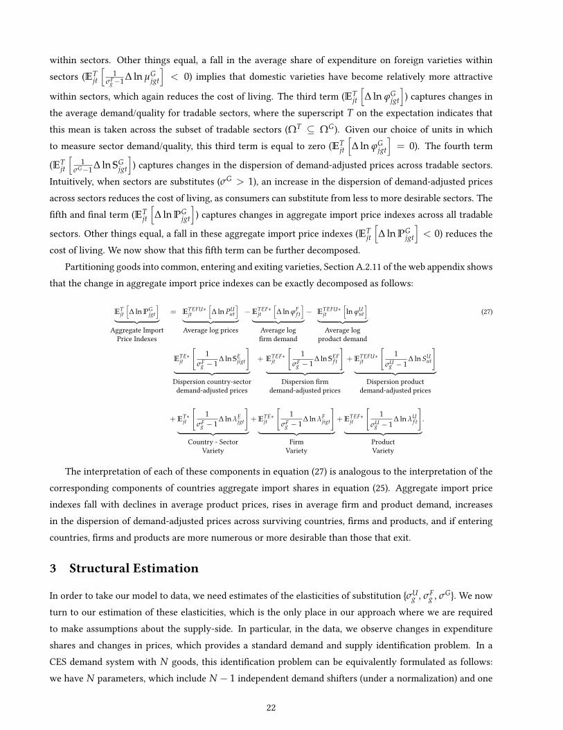
In addition to understanding aggregate trade patterns, researchers are often interested in understandingmovements in the aggregate cost of living, since this is important determinant of real income and welfare. InSection A.2.11 of the web appendix, we show that the change in the aggregate price index in equation (4) canbe exactly decomposed into the following ve terms:

∆ ln Pjt︸ ︷︷ ︸AggregatePrice Index

=1

σG − 1∆ ln µT

jt︸ ︷︷ ︸Non-Tradable

Competitiveness

+ ETjt

[1

σFg − 1

∆ ln µGjgt

]︸ ︷︷ ︸

DomesticCompetitiveness

+ ETjt

[∆ ln ϕG

jgt

]︸ ︷︷ ︸

AverageDemand

+ ETjt

[1

σG − 1∆ ln ST

jgt

]︸ ︷︷ ︸

Dispersion demand-adjusted prices across sectors

+ ETjt

[∆ ln PG

jgt

]︸ ︷︷ ︸

Aggregate ImportPrice Indexes

, (26)

where STjgt is the share of an individual tradable sector in expenditure on all tradable sectors. Recall that the

set of tradable sectors is constant over time and hence there are no terms for the entry and exit of sectors inequation (26).

The rst three terms capture shifts in aggregate prices that can be inferred from changes in market sharesor demand. The rst term ( 1

σG−1 ∆ ln µTjt) captures the relative attractiveness of varieties in the tradable and

non-tradable sectors. Other things equal, a fall in the share of expenditure on tradable sectors (∆ ln µIjt < 0)

implies that varieties in non-tradable sectors have become relatively more attractive, which reduces the costof living. The second term (ET

jt

[1

σFg−1 ∆ ln µG

jgt

]) captures the relative attractiveness of domestic varieties

21

within sectors. Other things equal, a fall in the average share of expenditure on foreign varieties withinsectors (ET

jt

[1

σFg−1 ∆ ln µG

jgt

]< 0) implies that domestic varieties have become relatively more attractive

within sectors, which again reduces the cost of living. The third term (ETjt

[∆ ln ϕG

jgt

]) captures changes in

the average demand/quality for tradable sectors, where the superscript T on the expectation indicates thatthis mean is taken across the subset of tradable sectors (ΩT ⊆ ΩG). Given our choice of units in whichto measure sector demand/quality, this third term is equal to zero (ET

jt

[∆ ln ϕG

jgt

]= 0). The fourth term

(ETjt

[1

σG−1 ∆ ln SGjgt

]) captures changes in the dispersion of demand-adjusted prices across tradable sectors.

Intuitively, when sectors are substitutes (σG > 1), an increase in the dispersion of demand-adjusted pricesacross sectors reduces the cost of living, as consumers can substitute from less to more desirable sectors. Thefth and nal term (ET

jt

[∆ ln PG

jgt

]) captures changes in aggregate import price indexes across all tradable

sectors. Other things equal, a fall in these aggregate import price indexes (ETjt

[∆ ln PG

jgt

]< 0) reduces the

cost of living. We now show that this fth term can be further decomposed.Partitioning goods into common, entering and exiting varieties, Section A.2.11 of the web appendix shows

that the change in aggregate import price indexes can be exactly decomposed as follows:

ETjt

[∆ ln PG

jgt

]︸ ︷︷ ︸

Aggregate ImportPrice Indexes

= ETEFU∗jt

[∆ ln PU

ut

]︸ ︷︷ ︸Average log prices

−ETEF∗jt

[∆ ln ϕF

f t

]︸ ︷︷ ︸

Average logrm demand

− ETEFU∗jt

[ln ϕU

ut

]︸ ︷︷ ︸

Average logproduct demand

(27)

ETE∗jt

[1

σFg − 1

∆ ln SEjigt

]︸ ︷︷ ︸Dispersion country-sectordemand-adjusted prices

+ ETEF∗jt

[1

σFg − 1

∆ ln SEFf t

]︸ ︷︷ ︸

Dispersion rmdemand-adjusted prices

+ ETEFU∗jt

[1

σUg − 1

∆ ln SUut

]︸ ︷︷ ︸

Dispersion productdemand-adjusted prices

+ ET∗jt

[1

σFg − 1

∆ ln λEjgt

]︸ ︷︷ ︸

Country - SectorVariety

+ ETE∗jt

[1

σFg − 1

∆ ln λFjigt

]︸ ︷︷ ︸

FirmVariety

+ ETEF∗jt

[1

σUg − 1

∆ ln λUf t

]︸ ︷︷ ︸

ProductVariety

.

The interpretation of each of these components in equation (27) is analogous to the interpretation of thecorresponding components of countries aggregate import shares in equation (25). Aggregate import priceindexes fall with declines in average product prices, rises in average rm and product demand, increasesin the dispersion of demand-adjusted prices across surviving countries, rms and products, and if enteringcountries, rms and products are more numerous or more desirable than those that exit.

3 Structural Estimation

In order to take our model to data, we need estimates of the elasticities of substitution σUg , σF

g , σG. We nowturn to our estimation of these elasticities, which is the only place in our approach where we are requiredto make assumptions about the supply-side. In particular, in the data, we observe changes in expenditureshares and changes in prices, which provides a standard demand and supply identication problem. In aCES demand system with N goods, this identication problem can be equivalently formulated as follows:we have N parameters, which include N − 1 independent demand shifters (under a normalization) and one

22

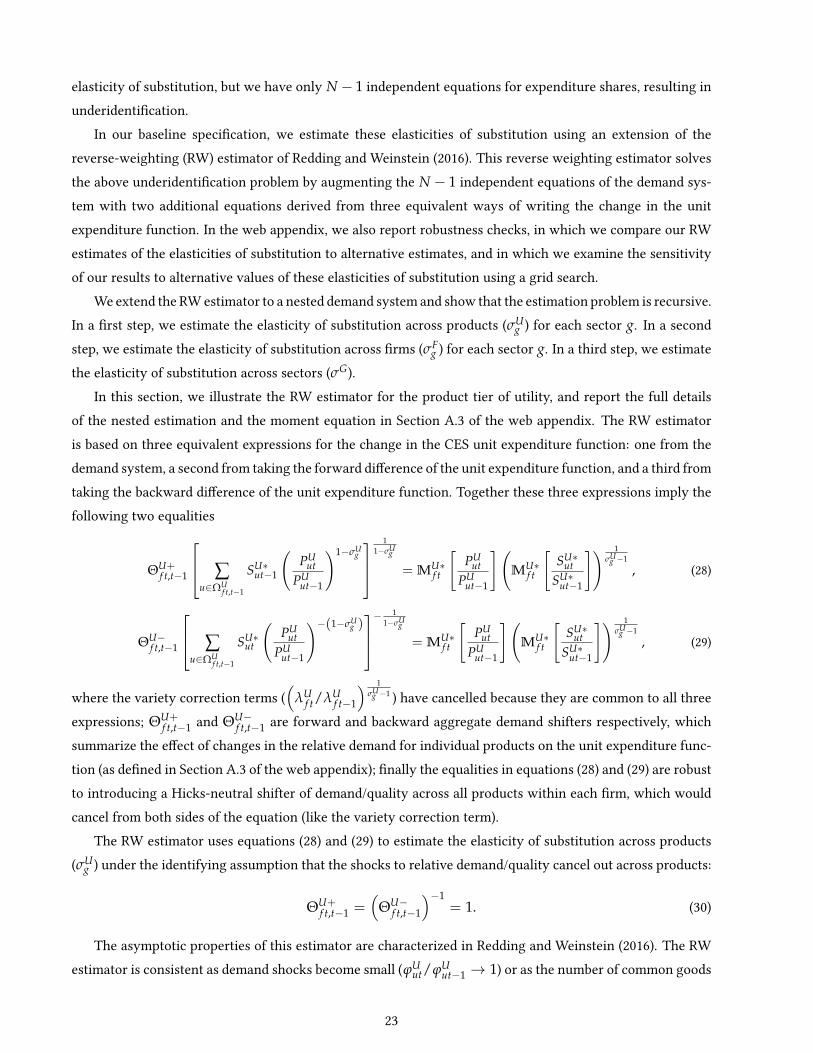
elasticity of substitution, but we have only N− 1 independent equations for expenditure shares, resulting inunderidentication.

In our baseline specication, we estimate these elasticities of substitution using an extension of thereverse-weighting (RW) estimator of Redding and Weinstein (2016). This reverse weighting estimator solvesthe above underidentication problem by augmenting the N − 1 independent equations of the demand sys-tem with two additional equations derived from three equivalent ways of writing the change in the unitexpenditure function. In the web appendix, we also report robustness checks, in which we compare our RWestimates of the elasticities of substitution to alternative estimates, and in which we examine the sensitivityof our results to alternative values of these elasticities of substitution using a grid search.

We extend the RW estimator to a nested demand system and show that the estimation problem is recursive.In a rst step, we estimate the elasticity of substitution across products (σU

g ) for each sector g. In a secondstep, we estimate the elasticity of substitution across rms (σF

g ) for each sector g. In a third step, we estimatethe elasticity of substitution across sectors (σG).

In this section, we illustrate the RW estimator for the product tier of utility, and report the full detailsof the nested estimation and the moment equation in Section A.3 of the web appendix. The RW estimatoris based on three equivalent expressions for the change in the CES unit expenditure function: one from thedemand system, a second from taking the forward dierence of the unit expenditure function, and a third fromtaking the backward dierence of the unit expenditure function. Together these three expressions imply thefollowing two equalities

ΘU+f t,t−1

∑u∈ΩU

f t,t−1

SU∗ut−1

(PU

utPU

ut−1

)1−σUg

1

1−σUg

= MU∗f t

[PU

utPU

ut−1

](MU∗

f t

[SU∗

utSU∗

ut−1

]) 1σU

g −1

, (28)

ΘU−f t,t−1

∑u∈ΩU

f t,t−1

SU∗ut

(PU

utPU

ut−1

)−(1−σUg )− 1

1−σUg

= MU∗f t

[PU

utPU

ut−1

](MU∗

f t

[SU∗

utSU∗

ut−1

]) 1σU

g −1

, (29)

where the variety correction terms ((

λUf t/λU

f t−1

) 1σU

g −1 ) have cancelled because they are common to all threeexpressions; ΘU+

f t,t−1 and ΘU−f t,t−1 are forward and backward aggregate demand shifters respectively, which

summarize the eect of changes in the relative demand for individual products on the unit expenditure func-tion (as dened in Section A.3 of the web appendix); nally the equalities in equations (28) and (29) are robustto introducing a Hicks-neutral shifter of demand/quality across all products within each rm, which wouldcancel from both sides of the equation (like the variety correction term).

The RW estimator uses equations (28) and (29) to estimate the elasticity of substitution across products(σU

g ) under the identifying assumption that the shocks to relative demand/quality cancel out across products:

ΘU+f t,t−1 =

(ΘU−

f t,t−1

)−1= 1. (30)

The asymptotic properties of this estimator are characterized in Redding and Weinstein (2016). The RWestimator is consistent as demand shocks become small (ϕU

ut/ϕUut−1 → 1) or as the number of common goods

23

becomes large and demand shocks are independently and identically distributed (NUt,t−1 → ∞). More gen-

erally, the identifying assumption in equation (30) is satised up to a rst-order approximation. Therefore,the RW estimator can be interpreted as providing a rst-order approximation to the data. In practice, we ndthat the RW estimated elasticities are similar to those estimated using other methods, such as the general-ization of the Feenstra (1994) estimator used in Hottman et al (2016). More generally, a key advantage of ourCES specication is that it is straightforward to undertake robustness checks to alternative values of theseelasticities of substitution using a grid search.

4 Data Description

To undertake our empirical analysis of the determinants of trade patterns and aggregate prices, we use inter-national trade transactions data that are readily available from customs authorities. In this section, we brieydiscuss the U.S. trade transactions data that we use in the paper, and report further details in Section A.4.1 ofthe web appendix. In Section A.4.2 of the web appendix, we discuss the Chilean trade transactions data thatwe use in robustness tests in the web appendix.

For each U.S. import customs shipment, we observe the cost inclusive of freight value of the shipment inU.S. dollars (market exchange rates), the quantity shipped, the date of the transaction, the product classi-cation (according to 10-digit Harmonized System (HS) codes), the country of origin, and a partner identiercontaining information about the foreign exporting rm.14 We concord the HS-digit 10-digit products to 4-digit sectors in the North American Industry Classication System (NAICS). We are thus able to construct adataset for a single importer j (the U.S.) with many exporters i (countries of origin), sectors g (4-digit NAICscodes), rms f (foreign rm identiers within exporters within sectors), and products u (10-digit HS codeswithin foreign rm identiers, within exporters and within sectors) and time t (year). We standardize theunits in which quantities are reported (e.g. we convert dozens to counts and grams to kilograms). We alsodrop any observations for which countries of origin or foreign rm identiers are missing. Finally, we collapsethe import shipments data to the annual level by exporting rm and product, weighting by trade value, whichyields a dataset on U.S. imports by source country (exporter), foreign rm, product and year from 1997-2011.In our nal year of 2011, we have over 3.7 million observations by exporter-rm-product.

Our measure of prices is the export unit value of an exporting rm within a 10-digit HS category. Whilethese data necessarily involve some aggregation across dierent varieties of products supplied by the same ex-porting rm within an observed product category, Section A.7 of the web appendix shows that our frameworkgeneralizes to the case in which rms make product decisions at a more disaggregated level than observedin the data. In this case, the product demand shifter (ϕU

ut) captures unobserved compositional dierenceswithin each observed product category. Moreover, 10-digit HS categories are relatively narrowly dened,and the coverage of sectors is much wider than in datasets that directly survey prices. As a result, manyauthors—including those working for statistical agencies—advocate for greater use of unit value data in the

14See Kamal, Krizan and Monarch (2015) for further discussion of the U.S. trade transactions data and comparisons of these partneridentiers using import data for the U.S. and export data from foreign countries. In robustness checks, we show that we continueto nd that the variety and average demand/quality terms dominate if we omit this partner identier (and focus only on countries,sectors and products) or use Chilean trade transactions data that report foreign brands.

24

construction of import price indexes.15 Furthermore, existing research comparing aggregate import price in-dexes constructed using unit values and directly surveyed prices nds only small dierences between them,as reported using U.S. data in Amiti and Davis (2009). Similarly, in our data we nd that the correlation be-tween a Cobb-Douglas price index (using lagged import shares as weights) and the BLS import price index is0.93, which suggests that unit value indexes capture much of the variation of import indexes based on pricequotes.

In Section A.5.5 of the web appendix, we show that our U.S. trade transactions data exhibit the sameproperties as found by a number of existing studies in the empirical trade literature.16 Two key features arethe high concentration of trade across countries and the dramatic increase in Chinese import penetration. Asshown in Figure A.5.5 of that section of the web appendix, the top 20 import source countries account foraround 80 percent of U.S. imports in each year; China’s import share more than doubles from 7 to 18 percentfrom 1997-2011; in contrast, Japan’s import share more than halves from 14 to 6 percent over this period.

5 Empirical Results

We present our results in several stages. We begin in Section 5.1 by reporting our estimates of the elasticitiesof substitution (σU

g , σFg , σG), which we use to invert the model and recover the values of product, rm and

sector demand/quality (ϕUut, ϕF

f t, ϕGjgt). In Section 5.2, we use these estimates to compute the exporter price

indexes that determine the cost of sourcing goods across countries and sectors. In Section 5.3, we report ourmain results for comparative advantage, aggregate trade and aggregate prices. In Section 5.4, we compare theresults of our framework with special cases that impose additional theoretical restrictions. In Section A.6 ofthe web appendix, we replicate all of these specication using our Chilean trade transactions data, and showthat we nd the same qualitative and quantitative pattern of results.

5.1 Elasticities of Substitution

In Table 1, we summarize our baseline estimates of the elasticities of substitution (σUg , σF

g , σG). Since weestimate a product and rm elasticity for each sector, it would needlessly clutter the paper to report all of theseelasticities individually. Therefore we report quantiles of the distributions of product and rm elasticities(σU

g , σFg ) across sectors and the single estimated elasticity of substitution across sectors (σG). The estimated

product and rm elasticities are signicantly larger than one statistically and always below eleven. We nd amedian estimated elasticity across products (σU

g ) of 6.29, a median elasticity across rms (σFg ) of 2.66, and an

elasticity across sectors (σG) of 1.36. These results imply that products within rms, rms within sectors andsectors are imperfect substitutes for one another, which has important implications for the measurement ofcomparative advantage below, because observed product prices are no longer sucient statistics for the costof sourcing goods across countries and sectors.

15For instance, Nakamura et al (2015) argue for the superiority of indexes based on disaggregated unit value data on theoreticalgrounds and “recommend alternatives to conventional price indexes that make use of unit values.”

16For example, see Bernard, Jensen and Schott (2009) and Bernard, Jensen, Redding and Schott (2009) for the U.S.; Mayer, Melitzand Ottaviano (2014) for France; and Manova and Zhang (2012) for China.

25

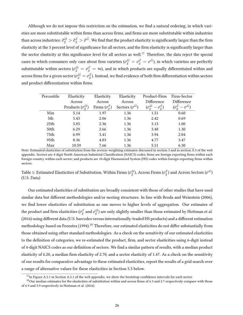
Although we do not impose this restriction on the estimation, we nd a natural ordering, in which vari-eties are more substitutable within rms than across rms, and rms are more substitutable within industriesthan across industries: σU

g > σFg > σG. We nd that the product elasticity is signicantly larger than the rm

elasticity at the 5 percent level of signicance for all sectors, and the rm elasticity is signicantly larger thanthe sector elasticity at this signicance level for all sectors as well.17 Therefore, the data reject the specialcases in which consumers only care about rm varieties (σU

g = σFg = σG), in which varieties are perfectly

substitutable within sectors (σUg = σF

g = ∞), and in which products are equally dierentiated within andacross rms for a given sector (σU

g = σFg ). Instead, we nd evidence of both rm dierentiation within sectors

and product dierentiation within rms.

Percentile Elasticity Elasticity Elasticity Product-Firm Firm-SectorAcross Across Across Dierence Dierence

Products (σUg ) Firms (σF

g ) Sectors (σG) (σUg − σF

g ) (σFg − σG)

Min 5.14 1.97 1.36 1.51 0.605th 5.43 2.06 1.36 2.42 0.6925th 5.85 2.36 1.36 3.13 1.0050th 6.29 2.66 1.36 3.48 1.3075th 6.99 3.41 1.36 3.94 2.0495th 8.36 4.83 1.36 4.77 3.47Max 10.59 7.66 1.36 5.51 6.30

Note: Estimated elasticities of substitution from the reverse-weighting estimator discussed in section 3 and in section A.3 of the webappendix. Sectors are 4-digit North American Industrial Classication (NAICS) codes; rms are foreign exporting rms within eachforeign country within each sector; and products are 10-digit Harmonized System (HS) codes within foreign exporting rms withinsectors.

Table 1: Estimated Elasticities of Substitution, Within Firms (σUg ), Across Firms (σF

g ) and Across Sectors (σG)(U.S. Data)

Our estimated elasticities of substitution are broadly consistent with those of other studies that have usedsimilar data but dierent methodologies and/or nesting structures. In line with Broda and Weinstein (2006),we nd lower elasticities of substitution as one moves to higher levels of aggregation. Our estimates ofthe product and rm elasticities (σF

g and σUg ) are only slightly smaller than those estimated by Hottman et al.

(2016) using dierent data (U.S. barcodes versus internationally-traded HS products) and a dierent estimationmethodology based on Feenstra (1994).18 Therefore, our estimated elasticities do not dier substantially fromthose obtained using other standard methodologies. As a check on the sensitivity of our estimated elasticitiesto the denition of categories, we re-estimated the product, rm, and sector elasticities using 6-digit insteadof 4-digit NAICS codes as our denition of sectors. We nd a similar pattern of results, with a median productelasticity of 6.20, a median rm elasticity of 2.70, and a sector elasticity of 1.47. As a check on the sensitivityof our results for comparative advantage to these estimated elasticities, report the results of a grid search overa range of alternative values for these elasticities in Section 5.3 below.

17In Figure A.5.1 in Section A.5.1 of the web appendix, we show the bootstrap condence intervals for each sector.18Our median estimates for the elasticities of substitution within and across rms of 6.3 and 2.7 respectively compare with those

of 6.9 and 3.9 respectively in Hottman et al. (2016).

26

5.2 Exporter Price Indexes Across Sectors and Countries

We use these estimated elasticities (σUg , σF

g , σG) to recover the structural residuals (ϕUut, ϕF

f t, ϕGjgt) and solve for

the exporter price indexes (PEjigt) that summarize the cost of sourcing goods from each exporter and sector.

A key implication of our framework is that these exporter price indexes depend not only on conventionalaverage price terms, but also on the non-conventional forces of average demand/quality, variety and thedispersion of demand-adjusted prices. We now quantify the relative importance of each of these componentsin our data.

In the four panels of Figure 2, we display a bin scatter of the log of the exporter price index (ln PEjigt) and

each of its components against average log product prices (EFUjigt

[ln PU

ut]), where the bins are twenty quantiles

of each variable.19 In each panel, we also show the regression relationship between the two variables basedon the disaggregated (i.e., not binned) data. For brevity, we show results for the nal year of our samplein 2011, but nd the same pattern for other years in our sample. In the top-left panel, we compare the logexporter price index (ln PE

jigt) to average log product prices (EFUjigt

[ln PU

ut]). In the special case in which

rms and products are perfect substitutes within sectors (σUg = σF

g = ∞) and there are no dierences indemand/quality (ϕF

f t = ϕFmt for all f , m and ϕU

ut = ϕU`t for all u, `), these two variables would be perfectly

correlated. In contrast to these predictions, we nd a positive but imperfect relationship, with an estimatedregression slope of 0.59 and R2 of 0.23. Therefore, the true cost of sourcing goods across countries and sectorscan dier substantially from standard empirical measures of average prices.

In the remaining panels of Figure 2, we explore the three sources of dierences between the exporterprice index and average log product prices. As shown in the top-right panel, exporter sectors with highaverage prices (horizontal axis) also have high average demand/quality (vertical axis), so that the impact ofhigher average prices in raising sourcing costs is partially oset by higher average demand/quality. Thispositive relationship between average prices and demand/quality is strong and statistically signicant, withan estimated regression slope of 0.41 and R2 of 0.28. This nding of higher average demand for productswith higher average prices is consistent with the quality interpretation of demand stressed in Schott (2004),in which producing higher quality incurs higher production costs.20

In measuring demand/quality as a residual that shifts expenditure shares conditional on price, we followa long line of research in trade and industrial organization. This approach is similar to that taken to measureproductivity in the growth literature, in which total factor productivity is a residual that shifts output con-ditional on inputs. The substantial variation in rm exports conditional on price is the underlying feature ofthe data that drives our nding of an important role for demand/quality in Figure 2. For plausible values ofthe elasticity of substitution, the model cannot explain this sales variation by price variation, and hence it isattributed to demand/quality. This result implies that the large class of trade models based on CES demandrequires heterogenous demand/quality and cost shifts in order to rationalize the data.

In the bottom-left panel of Figure 2, we show that the contribution from the number of varieties to the19We use a bin scatter, because U.S. Census disclosure requirements preclude showing results for each exporter-sector using the

U.S. data. In Section A.6.2 of the web appendix, we show results by exporter-sector using publicly-available Chilean data.20This close relationship between demand/quality and prices is consistent the ndings of a number of studies, including the

analysis of U.S. barcode data in Hottman et al. (2016) and the results for Chinese footwear producers in Roberts et al. (2011).

27

02

46

8Lo

g E

xpor

ter−

Sec

tor

Pric

e In

dex

0 2 4 6 8 10Average Log Prices

Note: Slope coefficient: 0.5901; standard error: 0.0135; R−squared: 0.2342.

Price Index Versus Average Prices

−3

−2

−1

01

2A

vera

ge L

og D

eman

d

0 2 4 6 8 10Average Log Prices

Note: Slope coefficient: 0.4055; standard error: 0.0105; R−squared: 0.2838.

Average Demand Versus Average Prices

.51

1.5

2V

arie

ty C

ontr

ibut

ion

0 2 4 6 8 10Average Log Prices

Note: Slope coefficient: 0.0064; standard error: 0.0064; R−squared: 0.0001.

Variety Versus Average Prices

−1.

2−

1−

.8−

.6−

.4D

ispe

rsio

n C

ontr

ibut

ion

0 2 4 6 8 10Average Log Prices

Note: Slope coefficient: 0.0020; standard error: 0.0039; R−squared: 0.0000.

Dispersion Versus Average Prices

Figure 2: U.S. Exporter-Sector Price Indexes and their Components Versus Average Log Product Prices, 2011

exporter-sector price index exhibits an inverse U-shape, at rst increasing with average prices, before laterdecreasing. This contribution ranges by more than two log points, conrming the empirical relevance ofconsumer love of variety. In contrast, in the bottom-right panel of Figure 2, we show that the contributionfrom the dispersion of demand-adjusted prices displays the opposite pattern of a U-shape, at rst decreas-ing with average prices before later increasing. While the extent of variation is smaller than for the varietycontribution, this term still uctuates by around half a log point between its minimum and maximum value.Therefore, the imperfect substitutability of rms and products implies important contributions from the num-ber of varieties and the dispersion in the characteristics of those varieties towards the true cost of sourcinggoods across countries and sectors.

These non-conventional determinants are not only important in the cross-section but are also importantfor changes in the cost of sourcing goods over time. A common empirical question in macroeconomics andinternational trade is the eect of price shocks in a given sector and country on prices and real economicvariables in other countries. However, it is not uncommon to nd that measured changes in prices oftenappear to have relatively small eects on real economic variables, which has stimulated research on “elasticitypuzzles” and the “exchange-rate disconnect.” Although duality provides a precise mapping between pricesand quantities, the actual price indexes used by researchers often dier in important ways from the formulasfor price indexes from theories of consumer behavior. For example, as we noted earlier, our average priceterm is the log of the “Jevons Index,” which is used by the U.S. Bureau of Labor Statistics (BLS) as part of itscalculation of the consumer price index. Except in special cases, however, this average price term will not

28

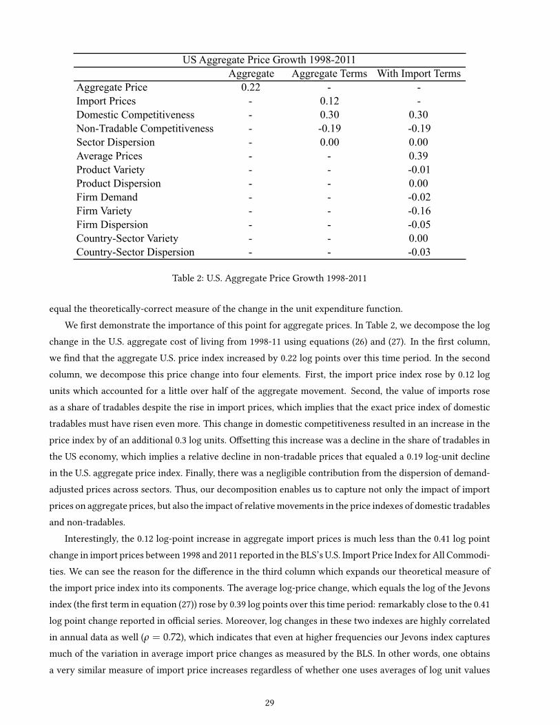
US Aggregate Price Growth 1998-2011Aggregate Aggregate Terms With Import Terms

Aggregate Price 0.22 - -Import Prices - 0.12 -Domestic Competitiveness - 0.30 0.30Non-Tradable Competitiveness - -0.19 -0.19Sector Dispersion - 0.00 0.00Average Prices - - 0.39Product Variety - - -0.01Product Dispersion - - 0.00Firm Demand - - -0.02Firm Variety - - -0.16Firm Dispersion - - -0.05Country-Sector Variety - - 0.00Country-Sector Dispersion - - -0.03

Table 2: U.S. Aggregate Price Growth 1998-2011

equal the theoretically-correct measure of the change in the unit expenditure function.We rst demonstrate the importance of this point for aggregate prices. In Table 2, we decompose the log

change in the U.S. aggregate cost of living from 1998-11 using equations (26) and (27). In the rst column,we nd that the aggregate U.S. price index increased by 0.22 log points over this time period. In the secondcolumn, we decompose this price change into four elements. First, the import price index rose by 0.12 logunits which accounted for a little over half of the aggregate movement. Second, the value of imports roseas a share of tradables despite the rise in import prices, which implies that the exact price index of domestictradables must have risen even more. This change in domestic competitiveness resulted in an increase in theprice index by of an additional 0.3 log units. Osetting this increase was a decline in the share of tradables inthe US economy, which implies a relative decline in non-tradable prices that equaled a 0.19 log-unit declinein the U.S. aggregate price index. Finally, there was a negligible contribution from the dispersion of demand-adjusted prices across sectors. Thus, our decomposition enables us to capture not only the impact of importprices on aggregate prices, but also the impact of relative movements in the price indexes of domestic tradablesand non-tradables.

Interestingly, the 0.12 log-point increase in aggregate import prices is much less than the 0.41 log pointchange in import prices between 1998 and 2011 reported in the BLS’s U.S. Import Price Index for All Commodi-ties. We can see the reason for the dierence in the third column which expands our theoretical measure ofthe import price index into its components. The average log-price change, which equals the log of the Jevonsindex (the rst term in equation (27)) rose by 0.39 log points over this time period: remarkably close to the 0.41log point change reported in ocial series. Moreover, log changes in these two indexes are highly correlatedin annual data as well (ρ = 0.72), which indicates that even at higher frequencies our Jevons index capturesmuch of the variation in average import price changes as measured by the BLS. In other words, one obtainsa very similar measure of import price increases regardless of whether one uses averages of log unit values

29

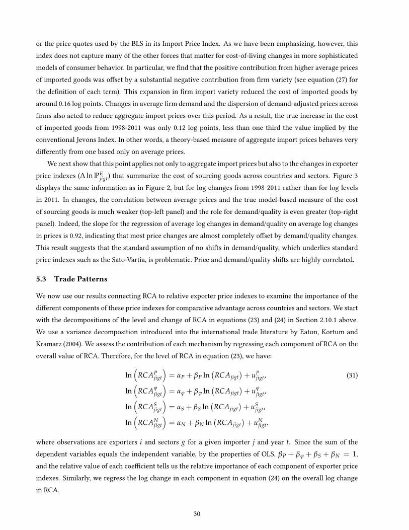
or the price quotes used by the BLS in its Import Price Index. As we have been emphasizing, however, thisindex does not capture many of the other forces that matter for cost-of-living changes in more sophisticatedmodels of consumer behavior. In particular, we nd that the positive contribution from higher average pricesof imported goods was oset by a substantial negative contribution from rm variety (see equation (27) forthe denition of each term). This expansion in rm import variety reduced the cost of imported goods byaround 0.16 log points. Changes in average rm demand and the dispersion of demand-adjusted prices acrossrms also acted to reduce aggregate import prices over this period. As a result, the true increase in the costof imported goods from 1998-2011 was only 0.12 log points, less than one third the value implied by theconventional Jevons Index. In other words, a theory-based measure of aggregate import prices behaves verydierently from one based only on average prices.

We next show that this point applies not only to aggregate import prices but also to the changes in exporterprice indexes (∆ ln PE

jigt) that summarize the cost of sourcing goods across countries and sectors. Figure 3displays the same information as in Figure 2, but for log changes from 1998-2011 rather than for log levelsin 2011. In changes, the correlation between average prices and the true model-based measure of the costof sourcing goods is much weaker (top-left panel) and the role for demand/quality is even greater (top-rightpanel). Indeed, the slope for the regression of average log changes in demand/quality on average log changesin prices is 0.92, indicating that most price changes are almost completely oset by demand/quality changes.This result suggests that the standard assumption of no shifts in demand/quality, which underlies standardprice indexes such as the Sato-Vartia, is problematic. Price and demand/quality shifts are highly correlated.

5.3 Trade Patterns

We now use our results connecting RCA to relative exporter price indexes to examine the importance of thedierent components of these price indexes for comparative advantage across countries and sectors. We startwith the decompositions of the level and change of RCA in equations (23) and (24) in Section 2.10.1 above.We use a variance decomposition introduced into the international trade literature by Eaton, Kortum andKramarz (2004). We assess the contribution of each mechanism by regressing each component of RCA on theoverall value of RCA. Therefore, for the level of RCA in equation (23), we have:

ln(

RCAPjigt

)= αP + βP ln

(RCAjigt

)+ uP

jigt, (31)

ln(

RCAϕjigt

)= αϕ + βϕ ln

(RCAjigt

)+ uϕ

jigt,

ln(

RCASjigt

)= αS + βS ln

(RCAjigt

)+ uS

jigt,

ln(

RCANjigt

)= αN + βN ln

(RCAjigt

)+ uN

jigt.

where observations are exporters i and sectors g for a given importer j and year t. Since the sum of thedependent variables equals the independent variable, by the properties of OLS, βP + βϕ + βS + βN = 1,and the relative value of each coecient tells us the relative importance of each component of exporter priceindexes. Similarly, we regress the log change in each component in equation (24) on the overall log changein RCA.

30

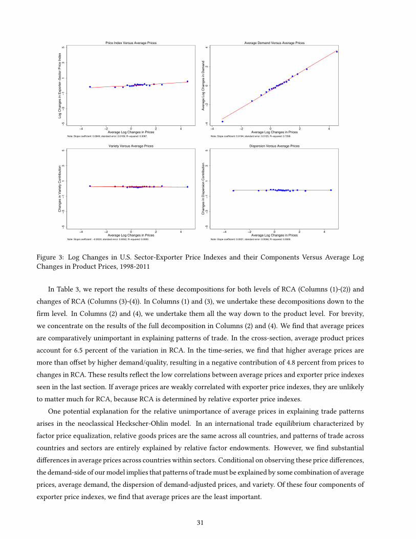
−5

−3

−1

13

5Lo

g C

hang

es in

Exp

orte

r−S

ecto

r P

rice

Inde

x

−4 −2 0 2 4Average Log Changes in Prices

Note: Slope coefficient: 0.0849; standard error: 0.0169; R−squared: 0.0087.

Price Index Versus Average Prices

−4

−2

02

4A

vera

ge L

og C

hang

es in

Dem

and

−4 −2 0 2 4Average Log Changes in Prices

Note: Slope coefficient: 0.9194; standard error: 0.0125; R−squared: 0.7299.

Average Demand Versus Average Prices

−5

−3

−1

13

5C

hang

es in

Var

iety

Con

trib

utio

n

−4 −2 0 2 4Average Log Changes in Prices

Note: Slope coefficient: −0.0024; standard error: 0.0052; R−squared: 0.0000.

Variety Versus Average Prices

−5

−3

−1

13

5C

hang

es in

Dis

pers

ion

Con

trib

utio

n

−4 −2 0 2 4Average Log Changes in Prices

Note: Slope coefficient: 0.0021; standard error: 0.0056; R−squared: 0.0000.

Dispersion Versus Average Prices

Figure 3: Log Changes in U.S. Sector-Exporter Price Indexes and their Components Versus Average LogChanges in Product Prices, 1998-2011

In Table 3, we report the results of these decompositions for both levels of RCA (Columns (1)-(2)) andchanges of RCA (Columns (3)-(4)). In Columns (1) and (3), we undertake these decompositions down to therm level. In Columns (2) and (4), we undertake them all the way down to the product level. For brevity,we concentrate on the results of the full decomposition in Columns (2) and (4). We nd that average pricesare comparatively unimportant in explaining patterns of trade. In the cross-section, average product pricesaccount for 6.5 percent of the variation in RCA. In the time-series, we nd that higher average prices aremore than oset by higher demand/quality, resulting in a negative contribution of 4.8 percent from prices tochanges in RCA. These results reect the low correlations between average prices and exporter price indexesseen in the last section. If average prices are weakly correlated with exporter price indexes, they are unlikelyto matter much for RCA, because RCA is determined by relative exporter price indexes.

One potential explanation for the relative unimportance of average prices in explaining trade patternsarises in the neoclassical Heckscher-Ohlin model. In an international trade equilibrium characterized byfactor price equalization, relative goods prices are the same across all countries, and patterns of trade acrosscountries and sectors are entirely explained by relative factor endowments. However, we nd substantialdierences in average prices across countries within sectors. Conditional on observing these price dierences,the demand-side of our model implies that patterns of trade must be explained by some combination of averageprices, average demand, the dispersion of demand-adjusted prices, and variety. Of these four components ofexporter price indexes, we nd that average prices are the least important.

31

Log Level RCA 2011 Log Change RCA 1998-11Firm-Level Product-Level Firm-Level Product-Level

Decomposition Decomposition Decomposition DecompositionFirm Price Index 0.094 - -0.005 -Firm Demand 0.220 0.220 0.422 0.422Firm Variety 0.324 0.324 0.501 0.501Firm Dispersion 0.362 0.362 0.082 0.082Product Prices - 0.065 - -0.048Product Variety - 0.014 - 0.037Product Dispersion - 0.014 - 0.007

Note: Variance decomposition for the log level of RCA in 2011 and the log change in RCA from 1998-2011 (from equation (31)).

Table 3: Variance Decomposition U.S. RCA

By contrast, we nd that average demand/quality is over three times more important than average prices,with a contribution of 22 percent for levels of RCA and 42 percent for changes in RCA in Table 3. Thisempirical nding for the relative importance of these two terms for patterns of trade is the reverse of therelative amount of attention devoted to them in existing theoretical research. In principle, one could rein-terpret the predictions of neoclassical trade models as predictions for relative prices after adjusting for de-mand/quality. However, we nd marked dierences in these average demand/quality-adjusted prices acrosscountries within sectors, implying substantial departures from goods price equalization even after makingthese adjustments. What sustains these dierences in adjusted prices in the model is the imperfect sub-stitutability of rms and products within sectors, which implies that both the number of varieties and thedispersion of demand-adjusted prices also matter for patterns of trade. Finally, it is not obvious that the de-terminants of quality/demand are the same as those of prices, with, for example, a large literature in industrialorganization emphasizing the importance of sunk costs for quality (e.g. Sutton 1991).

By far the most important of the dierent mechanisms for trade in Table 3 is rm variety, which accountsfor 32 and 50 percent of the level and change of RCA respectively. We also nd a substantial contributionfrom the dispersion of demand-adjusted prices across rms, particularly in the cross-section, where this termaccounts for 36 percent of the variation in RCA. In the time-series, this rm dispersion term is relatively lessimportant, though it still accounts for 8 percent of the variation in RCA. On the one hand, our ndings forrm variety are consistent with research that emphasizes the role of the extensive margin in understandingpatterns of trade (e.g. Hummels and Klenow 2005, Chaney 2008). On the other hand, our ndings for thedispersion of demand-adjusted prices across common varieties imply that the intensive margin is also im-portant (consistent with the analysis for a log normal distribution in Fernandes et al. 2015). In particular, wend quantitatively relevant dierences in the second moment of the distribution of demand-adjusted pricesacross common products and rms within exporters and sectors.

More broadly, this pattern of empirical results is consistent with theoretical frameworks in which compar-ative advantage operates not only through prices but also through the mass of rms and the distributions ofproductivity and demand across rms, such as Bernard, Redding, and Schott (2007). While recent empirical

32

studies have documented substantial churning in patterns of comparative advantage over time, as in Fre-und and Pierola (2015) and Hanson, Lind and Muendler (2016), our ndings imply that this churning largelyoccurs through changes in average demand/quality and rm entry/exit. The dominance of these two compo-nents of changes in average demand/quality and rm entry/exit points towards the relevance of theoreticalframeworks in which comparative advantage arises from endogenous investments in product and processinnovation, as in Grossman and Helpman (1991).

We nd that our results for comparative advantage are robust across a number of dierent specications.As a check on the sensitivity of our ndings to the denition of categories, we replicated our entire analysisusing a denition of sectors based of 6-digit instead of 4-digit NAICS codes. Using this dierent denition,we nd a similar pattern of results as in our baseline specication, with average demand/quality accountingfor 23 and 46 percent of the level and change of RCA, and rm variety making up 34 and 47 percent. As afurther robustness check, we undertook a grid search over the range of plausible values for the elasticities ofsubstitution across rms and products. In particular, we consider values of σF

g from 2 to 8 (in 0.5 increments)and values of σU

g from (σFg + 0.5) to 20 in 0.5 increments, while holding σG constant at our estimated value,

which respects our estimated ranking that σUg > σF

g > σG. As shown in Section A.5.3 of the web appendix,the contributions from rm variety and the dispersion of demand-adjusted prices across rms are invariantacross these parameter values, because the elasticities of substitution cancel from these two terms. In con-trast, the contributions from average prices and average demand/quality are increasing and decreasing in σF

g

respectively. Nevertheless, across the grid of parameter values, we nd that average prices account for lessthan 25 percent of the level of the RCA and less than 10 percent of the changes in RCA. Therefore, our ndingthat the relative price indexes that determine comparative advantage depart substantially from average pricesis robust across the range of plausible elasticities of substitution.

We now show that the non-conventional forces of variety, average demand/quality, and the dispersion ofdemand-adjusted prices are also important for understanding aggregate U.S. imports from its largest suppli-ers. In Figure 4, we show the time-series decompositions of aggregate import shares from equation (25) forthe top-ve trade partners of the United States. We nd that most of the increase in China’s market shareover the sample period occurs through increases in the number of rm varieties (orange), average rm de-mand/quality (dark gray) and the dispersion of demand-adjusted prices across rm varieties (light blue).21 Incontrast, average product prices (green) increased more rapidly for China than for the other countries in oursample, which worked to reduce China’s market share. Therefore, the reasons for the explosive growth ofChinese exports were not cheaper Chinese exports, but rather substantial rm entry (variety), demand/qualityupgrading, and improvements in the performance of leading rms relative to lagging rms (the dispersion ofdemand-adjusted prices). For Canada, we nd that rm exit (orange) makes the largest contribution to thedecline in its import share. For Germany, Japan and Mexico, we nd substantial contributions from averagerm demand/quality (gray) and the dispersion of demand-adjusted prices across rms (light blue), which arelarge relative to the contributions from average prices. Therefore, consistent with our results for sectoral

21Our nding of an important role for rm entry for China is consistent with the results for export prices in Amiti, Dai, Feenstra,and Romalis (2016). However, their price index is based on the Sato-Vartia formula, which abstracts from changes in demand/qualityfor surviving varieties, and they focus on Chinese export prices rather on than trade patterns.

33

------------

------------

------------

------------

------------

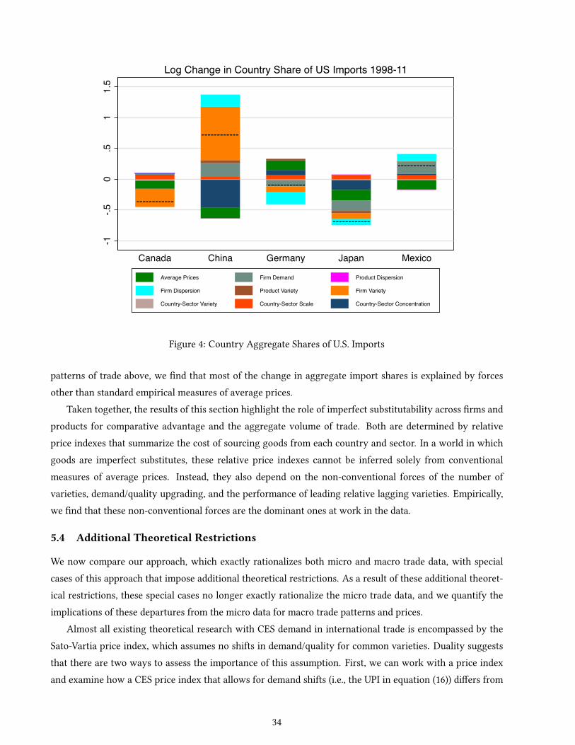
-1-.5

0.5

11.

5

Canada China Germany Japan Mexico

Log Change in Country Share of US Imports 1998-11

Average Prices Firm Demand Product Dispersion

Firm Dispersion Product Variety Firm Variety

Country-Sector Variety Country-Sector Scale Country-Sector Concentration

Figure 4: Country Aggregate Shares of U.S. Imports

patterns of trade above, we nd that most of the change in aggregate import shares is explained by forcesother than standard empirical measures of average prices.

Taken together, the results of this section highlight the role of imperfect substitutability across rms andproducts for comparative advantage and the aggregate volume of trade. Both are determined by relativeprice indexes that summarize the cost of sourcing goods from each country and sector. In a world in whichgoods are imperfect substitutes, these relative price indexes cannot be inferred solely from conventionalmeasures of average prices. Instead, they also depend on the non-conventional forces of the number ofvarieties, demand/quality upgrading, and the performance of leading relative lagging varieties. Empirically,we nd that these non-conventional forces are the dominant ones at work in the data.

5.4 Additional Theoretical Restrictions

We now compare our approach, which exactly rationalizes both micro and macro trade data, with specialcases of this approach that impose additional theoretical restrictions. As a result of these additional theoret-ical restrictions, these special cases no longer exactly rationalize the micro trade data, and we quantify theimplications of these departures from the micro data for macro trade patterns and prices.

Almost all existing theoretical research with CES demand in international trade is encompassed by theSato-Vartia price index, which assumes no shifts in demand/quality for common varieties. Duality suggeststhat there are two ways to assess the importance of this assumption. First, we can work with a price indexand examine how a CES price index that allows for demand shifts (i.e., the UPI in equation (16)) diers from

34

a CES price index that does not allow for demand shifts (i.e., the Sato-Vartia index). Since the common goodscomponent of the UPI (CG-UPI) and the Sato-Vartia indexes are identical in the absence of demand shifts,the dierence between the two is a metric for how important demand shifts are empirically. Second, wecan substitute each of these price indexes into equation (22) for revealed comparative advantage (RCA), andexamine how important the assumption of no demand shifts is for understanding patterns of trade. Sincethe UPI perfectly rationalizes the data, any deviation from the data arising from using a dierent price indexmust reect the eect of the restrictive assumption used in the index’s derivation. In order to make thecomparison fair, we need to also adjust the Sato-Vartia index for variety changes, which we do by using theFeenstra (1994) index, which is based on the same no-demand-shifts assumption for common goods, but addsthe variety correction term given in equation (16) to incorporate entry and exit.

In Figure 5, we report the results of these comparisons. The top two panels consider exporter priceindexes, while the bottom two panels examine RCA. In the top-left panel, we show a bin scatter of the Sato-Vartia exporter price index (on the vertical axis) against the common goods exporter price index (the CG-UPIon the horizontal axis), where the bins are twenty quantiles of each variable.22 We also show the regressionrelationship between the two variables based on the disaggregated (i.e. not binned) data. If the assumptionof time-invariant demand/quality were satised in the data, these two indexes would be perfectly correlatedwith one another and aligned on the 45-degree line. However, we nd little relationship between them. Thereason is immediately apparent if one recalls the top-right panel of Figure 3, which shows that price shifts arestrongly positively correlated with demand shifts. The Sato-Vartia price index fails to take into account thathigher prices are typically oset by higher demand/quality. In the top-right panel, we compare the Feenstraexporter price index (on the vertical axis) with our overall exporter price index (the UPI on the horizontal axis).These two price indexes have exactly the same variety correction term, but use dierent common goods priceindexes (the CG-UPI and Sato-Vartia indexes respectively). The importance of the variety correction termas a share of the overall exporter price index accounts for the improvement in the t of the relationship.However, the slope of the regression line is only around 0.5, and the regression R2 is about 0.1. Therefore,the assumption of no shifts in demand/quality for existing goods results in substantial deviations betweenthe true and measured costs of sourcing goods from an exporter and sector.

In the bottom left panel, we compare predicted changes in RCA based on relative exporter Sato-Vartiaprice indexes (on the vertical axis) against actual changes in RCA (on the horizontal axis). As the Sato-Vartia price index has only a weak correlation with the UPI, we nd that it has little predictive power forchanges in RCA, which are equal to relative changes in the UPI across exporters and sectors. Hence, observedchanges in trade patterns are almost uncorrelated with the changes predicted under the assumption of noshifts in demand/quality and no entry/exit of rms and products. In the bottom right panel, we compareactual changes in RCA (on the horizontal axis) against predicted changes in RCA based on relative exporterFeenstra price indexes (on the vertical axis). The improvement in the t of the relationship attests to theimportance of adjusting for entry and exit. However, again the slope of the regression line is only around

22Again we use a bin scatter, because U.S. Census disclosure requirements preclude showing results for each exporter-sector usingthe U.S. data. In Section A.6.4 of the web appendix, we show results by exporter-sector using publicly-available Chilean data.

35

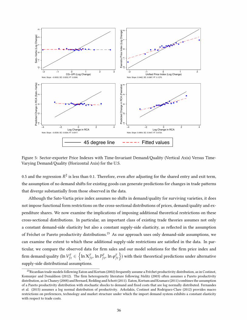
−2

−1

01

23

Sat

o−V

artia

(Lo

g C

hang

e)

−2 −1 0 1 2 3CG−UPI (Log Change)

Note: Slope: −0.0033; SE: 0.0252; R2: 0.0000.

−2

−1

01

2F

eens

tra

Pric

e In

dex

(Log

Cha

nge)

−2 −1 0 1 2Unified Price Index (Log Change)

Note: Slope: 0.5462; SE: 0.0387; R2: 0.1270.

−4

−2

02

4P

redi

cted

Cha

nge

in R

CA

(S

ato−

Var

tia)

−4 −2 0 2 4Log Change in RCA

Note: Slope: −0.0539; SE: 0.0334; R2: 0.0017.

−4

−2

02

4P

redi

cted

Cha

nge

in R

CA

(F

eens

tra)

−4 −2 0 2 4Log Change in RCA

Note: Slope: 0.4904; SE: 0.0447; R2: 0.0724.

45 degree line Fitted values

Figure 5: Sector-exporter Price Indexes with Time-Invariant Demand/Quality (Vertical Axis) Versus Time-Varying Demand/Quality (Horizontal Axis) for the U.S.

0.5 and the regression R2 is less than 0.1. Therefore, even after adjusting for the shared entry and exit term,the assumption of no demand shifts for existing goods can generate predictions for changes in trade patternsthat diverge substantially from those observed in the data.

Although the Sato-Vartia price index assumes no shifts in demand/quality for surviving varieties, it doesnot impose functional form restrictions on the cross-sectional distributions of prices, demand/quality and ex-penditure shares. We now examine the implications of imposing additional theoretical restrictions on thesecross-sectional distributions. In particular, an important class of existing trade theories assumes not onlya constant demand-side elasticity but also a constant supply-side elasticity, as reected in the assumptionof Fréchet or Pareto productivity distributions.23 As our approach uses only demand-side assumptions, wecan examine the extent to which these additional supply-side restrictions are satised in the data. In par-ticular, we compare the observed data for rm sales and our model solutions for the rm price index andrm demand/quality (ln VF

f t ∈

ln XFf t, ln PF

f t, ln ϕFf t

) with their theoretical predictions under alternative

supply-side distributional assumptions.23Ricardian trade models following Eaton and Kortum (2002) frequently assume a Fréchet productivity distribution, as in Costinot,

Komunjer and Donaldson (2012). The rm heterogeneity literature following Melitz (2003) often assumes a Pareto productivitydistribution, as in Chaney (2008) and Bernard, Redding and Schott (2011). Eaton, Kortum and Kramarz (2011) combines the assumptionof a Pareto productivity distribution with stochastic shocks to demand and xed costs that are log normally distributed. Fernandeset al. (2015) assumes a log normal distribution of productivity. Arkolakis, Costinot and Rodriguez-Clare (2012) provides macrorestrictions on preferences, technology and market structure under which the import demand system exhibits a constant elasticitywith respect to trade costs.

36

To derive these theoretical predictions, we use the QQ estimator of Kratz and Resnick (1996), as introducedinto the international trade literature by Head, Mayer and Thoenig (2016). This QQ estimator compares theempirical quantiles in the data with the theoretical quantiles implied by alternative distributional assumptions.As shown in Section A.5.4 of the web appendix, under the assumption that VF

f t has an untruncated Paretodistribution, we obtain the following theoretical prediction for the quantile of the logarithm of that variable:

ln(

VFf t

)= ln VF

jigt −1

aVg

ln[1−Fjigt

(VF

f t

)], (32)

whereFjigt (·) is the cumulative distribution function; ln VFjigt is the lower limit of the support of the untrun-

cated Pareto distribution, which is a constant across rms f for a given importer j, exporter i, sector g andyear t; aV

g is the shape parameter of this distribution, which we allow to vary across sectors g.We estimate equation (32) by OLS using the empirical quantile for ln

(VF

f t

)on the left-hand side and the

empirical estimate of the cumulative distribution function forFjigt

(VF

f t

)on the right-hand side, as discussed

further in the web appendix. We estimate this regression for each sector across foreign rms (allowing theslope coecient aV

g to vary across sectors) and including xed eects for each exporter-year-sector combi-nation (allowing the intercept ln VF

jigt to vary across exporters, sectors and time). The tted values from thisregression correspond to the predicted theoretical quantiles, which we compare to the empirical quantilesobserved in the data. Under the null hypothesis of a Pareto distribution, there should be a linear relationshipbetween the theoretical and empirical quantiles that coincides with the 45-degree line.

To assess the empirical validity of this theoretical prediction, we estimate equation (32) for two separatesubsamples: rms with values below the median for each exporter-sector-year cell and rms with valuesabove the median for each exporter-sector-year cell. Under the null hypothesis of a Pareto distribution, theestimated slope coecient 1/aV

g should be the same for rms below and above the median.24 As shown inSection A.5.4 of the web appendix, we strongly reject this null hypothesis of a Pareto distribution for all threevariables, with substantial dierences in the estimated coecients below and above the median, which arestatistically signicant at conventional levels.25

To provide a point of comparison, we also consider the log-normal distributional assumption. As shownin Section A.5.4 of the web appendix, we obtain the following theoretical prediction for the quantile of thelogarithm of a variable VF

f t under this distributional assumption:

ln(

VFf t

)= κV

jigt + χVg Φ−1

(Fjigt

(VF

f t

)). (33)

where Φ−1 (·) is the inverse of the normal cumulative distribution function; κVjigt and χV

g are the mean and

standard deviation of the log variable, such that ln(

VFf t

)∼ N

(κV

jigt,(

χVg

)2)

; we make analogous assump-tions about these two parameters as for the untruncated Pareto distribution above; we allow the parametercontrolling the mean (κV

jigt) to vary across exporters i, sectors g and time t for a given importer j; we allowthe parameter controlling dispersion (χV

g ) to vary across sectors g.24U.S. Census disclosure requirements preclude showing the quantiles for individual foreign rms using the U.S. data. In Figures

A.6.7 and A.6.8 in Section A.6.4 of the web appendix, we show rm quantiles using publicly-available Chilean data.25A similar analysis can be undertaken for a Fréchet distribution. We nd a similar pattern of statistically signicant departures

from the predicted linear relationship between the theoretical and empirical quantiles under this distributional assumption.

37

Again we estimate equation (33) by OLS using the empirical quantile for ln(

VFf t

)on the left-hand side

and the empirical estimate of the cumulative distribution function for Fjigt

(VF

f t

)on the right-hand side.

We estimate this regression for each sector across foreign rms (allowing the slope coecient χVg to vary

across sectors) and including xed eects for each exporter-year-sector combination (allowing the interceptκV

jigt to vary across exporters, sectors and time). As shown in Section A.5.4 of the web appendix, we ndthat the log-normal distributional assumption provides a closer approximation to the data than the Paretodistributional assumption. Consistent with Bas, Mayer and Thoenig (2017), we nd smaller departures fromthe predicted linear relationship between the theoretical and empirical quantiles for a log-normal distributionthan for a Pareto distribution. Nevertheless, we reject the null hypothesis of a log-normal distribution at con-ventional signicance levels for all three variables for the majority of industries, with substantial dierencesin estimated coecients above and below the median. Instead of imposing such supply-side distributionalassumptions, our demand-side approach uses the observed empirical distributions of prices and expenditureshares, and the resulting implied distribution of demand/quality under our assumption of CES demand.

As a concluding point, we examine the implications of these departures from a Pareto and log-normaldistributions for understanding trade patterns across countries and sectors. Here, we demonstrate a surpris-ing result. If one rationalizes the data using the unied price index, distributional assumptions about theunderlying parameters do not matter, as long as these distributions are centered on the correct mean of thelogs of each variable. To see this, we take the mean of the predicted values for log rm import shares, logrm-price indexes and log rm-demand/quality, and use our estimated elasticities of substitution to constructthe predicted log common-goods unied price index for each exporter and sector:

ln PEjigt = EF

jigt

[ln PF

f t

]−EF

jigt

[ln ϕF

f t

]+

1σF

g − 1EF

jigt

[ln SEF

f t

], (34)

where a hat above a variable denotes a predicted value (recall that SEFf t is the share of each rm f ∈ ΩF

jigt incounty j’s imports from a given exporter i 6= j in sector g at time t).

A notable feature of this equation is that if we remove the hats, we obtain the exporter price index, whichrationalizes revealed comparative advantage exactly. In this case, each of the terms on the right-hand sidecorrespond the means of the logs of each variable. It follows immediately from this that that any distributionof the log of prices, demand/quality parameters, and shares that has the same means as in the data will producethe correct exporter price index and match RCA. Given our inclusion of exporter-sector-year xed eects inequations (32) and (33), both of the estimated distributions are centered on the correct means of the logs ofeach variable for each exporter-sector-year. Therefore, these distributional assumptions do not matter for ourconclusions about the sources of variation of RCA, as long as they implemented in such a way as to preservethe correct means of the logs of each variable for each exporter-sector-year.

6 Conclusions

One of the earliest stylized facts in international economics is that aggregate import prices and import vol-umes have correlations that are often the wrong sign or close to zero. Economists have long known the two

38

main reasons for this nding: “shifts in the demand schedule” and “faulty methods of price index construc-tion.” We develop a method for accounting for movements in aggregate import price indexes and trade owsthat allows for shifts in demand, prices, quality, variety and rm heterogeneity or dispersion. Our approachuses the invertibility of the CES demand system to recover unobserved values of demand/quality that ex-actly rationalize disaggregated trade data. We show how to aggregate to the national level even when dataare incomplete or missing using a log-linear representation that permits exact decompositions of aggregatevariables.

Unlike prior import price indexes, our indexes allow not only for changes in prices and variety, but alsoinnovations in the demand for and quality of existing goods. We show that our average price term has asimilar functional form and turns out to be highly correlated with the BLS import price index. But the otherterms in our price index have very dierent functional forms and turn out to be negatively correlated withthe BLS import price index. The importance of these other terms helps to explain the diculty of trying tounderstand trade patterns using only conventional measures of import and domestic prices.

We derive a theoretically-rigorous measure of revealed comparative advantage (RCA) that depends onthe relative values of our price indexes across countries and sectors. This RCA measure is also additivelyseparable into price, demand/quality, entry/exit and dispersion terms in both the cross-section and time-series. We show that rm entry/exit and average demand/quality each account for around 45 percent of thetime-series variation in imports, with the dispersion of demand-adjusted prices making up most of the rest.We show that these same factors account for most of the growth of China’s share of aggregate U.S. imports,in spite of a relative increases in Chinese export prices.

Although there is an exact mapping between our price indexes and observed trade ows, the same neednot be true for other approaches that impose stronger assumptions. We show that models that assume nodemand shifts and no changes in variety perform poorly on international trade data. Models that accountfor variety changes while maintaining the assumption of no demand shifts do better, but still account foronly about ten percent of the changes in comparative advantage over time. Finally, we provide new evidenceon the empirical relevance of standard distributional assumptions (such as Pareto, Fréchet or log normal)for understanding patterns of international trade and import prices. Remarkably, we show that under CESdemand it does not matter what the underlying productivity distribution is as long as it is correctly centeredsuch that it matches the geometric average price, quality and sales of each rm.

References

[1] Adler, J. Hans (1945) “United States Import Demand During the Interwar Period,” The American EconomicReview, 35(3), 418-430.

[2] Adao, Rodrigo, Arnaud Costinot and Dave Donaldson (2017) “Nonparametric Counterfactual Predictionsin Neoclassical Models of International Trade,” American Economic Review, 107(3), 633-689.

[3] Amiti, Mary, Mi Dai, Robert Feenstra, and John Romalis (2016) “How Did China’s WTO Entry BenetU.S. Consumers?”, UC Davis, mimeograph.

39

[4] Amiti, Mary and Donald R. Davis (2009) “What’s Behind Volatile Import Prices from China?,” CurrentIssues in Economics and Finance, 15(1), 1-7.

[5] Arkolakis, Costas, Arnaud Costinot and Andres Rodriguez-Clare (2012) “New Trade Models, Same OldGains,” American Economic Review, 102(1), 94-130.

[6] Armington, Paul S. (1969) “A Theory of Demand for Products Distinguished by Place of Production,”International Monetary Fund Sta Papers, 16(1), 159–78.

[7] Atkeson, Andrew, and Ariel Burstein (2008) “Pricing to Market, Trade Costs and International RelativePrices,” American Economic Review, 98, 1998-2031.

[8] Atkin, David, and Dave Donaldson (2015) “Who’s Getting Globalized? The Size and Implications ofIntra-national Trade Costs,” NBER Working Paper, 21439.

[9] Atkin, David, Benjamin Faber and Marco Gonzalez-Navarro (2016) “Retail Globalization and HouseholdWelfare: Evidence from Mexico,” Journal of Political Economy, forthcoming.

[10] Balassa, Bela (1965) “Trade Liberalization and Revealed Comparative Advantage,” Manchester School ofEconomic and Social Studies, 33, 99-123.

[11] Bas, Maria, Thierry Mayer and Mathias Thoenig (2017) “From Micro to Macro: Demand, Supply andHeterogeneity in the Trade Elasticity,” Journal of International Economics, 108, 1-19.

[12] Bernard, Andrew. B., and J. Bradford Jensen (1995) “Exporters, Jobs, and Wages in US Manufacturing:1976-87,” Brookings Papers on Economic Activity: Microeconomics, 67-112.

[13] Bernard, Andrew B., J. Bradford Jensen, and Peter K. Schott (2009) “Importers, Exporters and Multina-tionals: A Portrait of Firms in the U.S. that Trade Goods,” in Producer Dynamics: New Evidence fromMicroData, ed. by T. Dunne, J. B. Jensen, and M. J. Roberts. Chicago University Press, Chicago.

[14] Bernard, Andrew B., J. Bradford Jensen, Stephen J. Redding, and Peter K. Schott (2007) “Firms in Inter-national Trade,” Journal of Economic Perspectives, 21(3), 105-130.

[15] Bernard, Andrew B., J. Bradford Jensen, Stephen J. Redding, and Peter K. Schott (2009) “The Margins ofU.S. Trade,” American Economic Review, Papers and Proceedings, 99(2), 487-493.

[16] Bernard, Andrew B., Stephen J. Redding and Peter K. Schott (2007) “Comparative Advantage and Het-erogeneous Firms,” Review of Economic Studies, 74(1), 31-66.

[17] Bernard, Andrew B., Stephen J. Redding and Peter K. Schott (2010) “Multi-product Firms and ProductSwitching,” American Economic Review, 100(1), 70– 97.

[18] Bernard, Andrew B., Stephen J. Redding and Peter K. Schott (2011) “Multiproduct Firms and Trade Lib-eralization,” Quarterly Journal of Economics, 126(3), 1271-1318.

[19] Broda, Christian and David E. Weinstein (2006) “Globalization and the Gains from Variety,” QuarterlyJournal of Economics, 121, 541-86.

[20] Broda, Christian and David E. Weinstein (2010) “Product Creation and Destruction: Evidence and PriceImplications,” American Economic Review, 100, 691-723.

[21] Caliendo, Lorenzo and Fernando Parro (2015) “Estimates of the Trade and Welfare Eects of NAFTA,”Review of Economic Studies, 82 (1), 1-44.

40

[22] Chaney, Thomas (2008) “Distorted Gravity: The Intensive and Extensive Margins of International Trade,”American Economic Review, 98(4), 1707-1721.

[23] Costinot, Arnaud, Dave Donaldson and Ivana Komunjer (2012) “What Goods Do Countries Trade? AQuantitative Exploration of Ricardo’s Ideas,” Review of Economic Studies, 79, 581-608.

[24] Crozet, Matthieu, Keith Head, and Thierry Mayer (2012) “Quality Sorting and Trade: Firm-level Evidencefor French Wine,” Review of Economic Studies, 79(2): 609-644.

[25] De Loecker, Jan and Penny Goldberg (2014) “Firm Performance in a Global Market,” Annual Review ofEconomics, 6, 201-227.

[26] Dhingra, Swati (2013) “Trading Away Wide Brands for Cheap Brands,”American Economic Review, 103(6),2554-84.

[27] Di Comite, F., Thisse, J., Vandenbussche, H. (2014). “Verti-zontal Dierentiation in Export Markets”,Journal of International Economics, 93, 50-66.

[28] Eaton, Jonathan and Samuel S. Kortum (2002) “Technology, Geography, and Trade,” Econometrica, 70(5),1741-1779.

[29] Eaton, Jonathan, Samuel S. Kortum and Francis Kramarz (2004) “Dissecting Trade: Firms, Industries, andExport Destinations,” American Economic Review, Papers and Proceedings, 94(2), 150–154.

[30] Eaton, Jonathan, Samuel S. Kortum and Francis Kramarz (2011) “An Anatomy of International Trade:Evidence from French Firms,” Econometrica, 79(5), 1453–1498.

[31] Eckel, Carsten and J. Peter Neary (2010) “Multi-product Firms and Flexible Manufacturing in the GlobalEconomy,” Review of Economic Studies, 77, 188-217.

[32] Fally, Thibault and Benjamin Faber (2016) “Firm Heterogeneity in Consumption Baskets: Evidence fromHome and Store Scanner Data,” University of California, Berkeley, mimeograph.

[33] Feenstra, Robert C. (1994) “New Product Varieties and the Measurement of International Prices,” Amer-ican Economic Review, 84, 157-177.

[34] Feenstra, Robert C. and Hong Ma “Optimal Choice of Product Scope for Multiproduct Firms,” in TheOrganization of Firms in a Global Economy, in (eds) Elhanan Helpman, Dalia Marin and Thierry Verdier,chapter 6, 173-199. Cambridge MA: Harvard University Press.

[35] Feenstra, Robert C., Philip Luck, Maurice Obstfeld, and Katheryn N. Russ (2014) “In Search of the Arm-ington Elasticity,” Review of Economics and Statistics, forthcoming.

[36] Feenstra, Robert C. and John Romalis (2014) “International Prices and Endogenous Quality,” QuarterlyJournal of Economics, 129(2), 477-527.

[37] Fernandes, Ana, Peter Klenow, Martha Denisse Pierola, Andres Rodriguez-Clare and Sergii Meleshchuk(2015) “The Intensive Margin in Trade,” Stanford University, mimeograph.

[38] Foster, Lucia, John Haltiwanger and Chad Syverson (2008) “Reallocation, Firm Turnover, and Eciency:Selection on Productivity or Protability?” American Economic Review, 98(1), 394-425.

[39] Freund, Caroline and Martha Denisse Pierola (2015) “Export Superstars,” Review of Economics and Statis-tics, 97(5), 1023-32.

41

[40] Grossman, Gene and Elhanan Helpman (1991) Innovation and Growth in the Global Economy, Cambridge:MIT Press.

[41] Hallak, Juan Carlos and Peter K. Schott (2011) “Estimating Cross-Country Dierences in Product Qual-ity,” Quarterly Journal of Economics, 126, 417-474.

[42] Handbury, Jessie (2013) “Are Poor Cities Cheap for Everyone? Non-Homotheticity and the Cost of LivingAcross U.S. Cities,” the Wharton School, University of Pennsylvania.

[43] Hanson, Gordon H., Nelson Lind and Marc-Andreas Muendler (2015) “The Dynamics of ComparativeAdvantage,” NBER Working Paper, 21753.

[44] Head, Keith, Thierry Mayer and Mathias Thoenig (2014) “Welfare and Trade Without Pareto,” AmericanEconomic Review, Papers and Proceedings, 104(5), 310-316.

[45] Hottman, Colin, Stephen J. Redding and David E. Weinstein (2016) “Quantifying the Sources of FirmHeterogeneity,” Quarterly Journal of Economics, 131(3), 1291-1364.

[46] Hsieh, Chang-Tai, Nicholas Li, Ralph Ossa, and Mu-Jeung Yang (2016) “Accounting for the Gains fromTrade Liberalization,” University of Chicago, mimeograph.

[47] Hummels, David and Peter J. Klenow (2005) “The Variety and Quality of a Nation’s Exports,” AmericanEconomic Review, 95(3), 704-723.

[48] Kamal, Fariha, C. J. Krizan and Ryan Monarch (2015) “Identifying Foreign Suppliers in U.S. MerchandiseImport Transactions”, Center for Economic Studies Working Paper, 15-11, Bureau of the Census.

[49] Kehoe, Timothy J. and Ruhl, Kim J. (2013) “How Important is the New Goods Margin in InternationalTrade,” Journal of Political Economy, 121(2) 2013.

[50] Khandelwal, Amit K. (2010) “The Long and Short (of) Quality Ladders,” Review of Economic Studies, 77,1450-1476.

[51] Kratz, Marie, and Sidney I Resnick (1996) “The QQ-estimator and Heavy Tails,” Stochastic Models, 12(4),699-724.

[52] Krugman, Paul (1980) “Scale Economies, Product Dierentiation, and the Pattern of Trade,” AmericanEconomic Review, 70(5), 950-959.

[53] Levchenko, Andrei A. and Jing Zhang (2016) “The Evolution of Comparative Advantage: Measurementand Welfare Implications,” Journal of Monetary Economics, 78, 96-111.

[54] Manova, Kalina and Zhiwei Zhang (2012) “Export Prices across Firms and Destinations,” Quarterly Jour-nal of Economics, 127, 379-436.

[55] Mayer, Thierry, Marc Melitz and Gianmarco I. P. Ottaviano (2014) “Market Size, Competition, and theProduct Mix of Exporters,” American Economic Review, 104(2), 495-536.

[56] Melitz, Marc J. (2003) “The Impact of Trade on Intra-Industry Reallocations and Aggregate IndustryProductivity,” Econometrica, 71, 1695-1725.

[57] Melitz, Marc J. and Stephen J. Redding (2014) “Heterogeneous Firms and Trade,” in Handbook of Interna-tional Economics, ed. by E. Helpman, G. Gopinath, and K. Rogo, vol. 4, chapter 1, 1-54, Elsevier, NorthHolland: Amsterdam.

42

[58] Nakamura, Alice, W. Erwin Diewert, John S. Greenlees, Leonard I. Nakamura, and Marshall B. Reins-dorf (2015) “Sourcing Substitution and Related Price Index Biases,” in Susan N. Houseman and MichaelMandel (eds.), Measuring Globalization: Better Trade Statistics for Better Policy, Volume 1, Biases to Price,Output, and Productivity Statistics from Trade W.E. Upjohn Institute for Employment Research, 21-88.

[59] Redding, Stephen J. and David E. Weinstein (2016) “A Unied Approach to Estimating CES Demand andWelfare,” NBER Working Paper, 22479.

[60] Roberts, Mark J., Xiaoyan Fan, Daniel Xu and Shengxing Zhang (2011) “A Structural Model of Demand,Cost, and Export Market Selection for Chinese Footwear Producers,” NBER Working Paper, 17725.

[61] Schott, Peter K. (2004) “Across-product Versus Within-product Specialization in International Trade,”Quarterly Journal of Economics, 119, 647-678.

[62] Sutton, John (1991) Sunk Costs and Market Structure: Price Competition, Advertising, and the Evolution ofConcentration, Cambridge MA: MIT Press.

[63] Sutton, John and Daniel Treer (2016) “Capabilities, Wealth, and Trade,” Journal of Political Economy,124(3), 826-878.

43