accuracy assessment of coastal topography derived from uav

ACCURACY ASSESSMENT OF COASTAL TOPOGRAPHY DERIVED FROM UAV IMAGES

N. Long a, *, B. Millescamps a, F. Pouget a, A. Dumon a, N. Lachaussée a, X. Bertin a

a Littoral, Environnement et Sociétés, Université de la Rochelle – CNRS, 2 rue Olympe de Gouges, 17 000 La Rochelle, France

(nathalie.long, bastien.millescamps, frederic.pouget, antoine.dumon, nicolas.lachaussee, xavier.bertin)@univ-lr.fr

ThS11

KEY WORDS: Digital Surface Model, Coastal monitoring, UAV photogrammetry, Accuracy ABSTRACT To monitor coastal environments, Unmanned Aerial Vehicle (UAV) is a low-cost and easy to use solution to enable data acquisition with high temporal frequency and spatial resolution. Compared to Light Detection And Ranging (LiDAR) or Terrestrial Laser Scanning (TLS), this solution produces Digital Surface Model (DSM) with a similar accuracy. To evaluate the DSM accuracy on a coastal environment, a campaign was carried out with a flying wing (eBee) combined with a digital camera. Using the Photoscan software and the photogrammetry process (Structure From Motion algorithm), a DSM and an orthomosaic were produced. Compared to GNSS surveys, the DSM accuracy is estimated. Two parameters are tested: the influence of the methodology (number and distribution of Ground Control Points, GCPs) and the influence of spatial image resolution (4.6 cm vs 2 cm). The results show that this solution is able to reproduce the topography of a coastal area with a high vertical accuracy (< 10 cm). The georeferencing of the DSM require a homogeneous distribution and a large number of GCPs. The accuracy is correlated with the number of GCPs (use 19 GCPs instead of 10 allows to reduce the difference of 4 cm); the required accuracy should be dependant of the research problematic. Last, in this particular environment, the presence of very small water surfaces on the sand bank does not allow to improve the accuracy when the spatial resolution of images is decreased. * Corresponding author – Nathalie Long, [email protected]; +33-05-46-50-76-33

1. INTRODUCTION

Natural mechanisms maintain coastal systems where marine and terrestrial processes are in interactions (Aidy et al., 2007). Sea level changes, storms waves can affect coastal environments, inducing erosion or sedimentation. For monitoring the coastal morphology, accurate and affordable data is necessary to improve the knowledge about topographic processes and evolution. Accurate topographic/bathymetric measurements are also required to perform numerical simulations of tides, waves and related sediment transport and morphological changes. Accurate data sources have to be available and the methodology has to be adapted to spatial and temporal resolutions (Thieler and Danforth, 1994, Quartel et al., 2007, Pardo-Pascual et al., 2012, Ford, 2013). Currently, several approaches are used to acquire spatial information about coastal topography. Satellite images are widely used in coastal studies and can provide a coastal change history (Chaumillon et al., 2014, Long et al., 2014). Applications of remote sensing have proved particularly effective in the delineation of coastal configuration, coastal landforms, and landform changes (Ryu et al., 2002; Maiti and Bhattacharya, 2009) but temporal frequency of images acquisition and/or spatial resolution of images can be limiting. Other techniques like Light Detection And Ranging (LiDAR) or Terrestrial Laser Scanning (TLS) can provide very high resolution and accurate data but are typically expensive (White and Wang, 2003; Nagihara et al., 2004; Letortu et al., 2015). To improve temporal frequency of data acquisition, Unmanned Aerial Vehicle (UAV) combined with a digital camera is a solution for coastal monitoring. Limited by the meteorological conditions (wind speed inferior to 70-80 km/h and no rain) and the study area size (typically of the order of 1km²), UAV and

photogrammetric process present advantage to generate 3D point cloud and Digital Surface Model (DSM) with accuracy closed to LiDAR DSM (Haala, 2009). Several studies have demonstrated the performance of this survey process on coastal areas (Casella et al., 2016; Gonçalves and Henriques, 2015; Casella et al., 2014; Mancini et al., 2013) with a vertical accuracy of the DEM around +/- 10 cm. Atlantic European coasts are exposed to winter storms which cause erosion and coastal damages (Castelle et al., 2015; Taveira-Pinto et al., 2011). In France, retreat of the coastline can reach several tens of meters per season (Bertin et al., 2008) and rapid morphological changes can be observed on sandy beaches, and more particularly on the Pertuis Charentais coast (central part of the Bay of Biscay). These rapid and substantial evolutions impact infrastructure beachfront, with significant socio-economic consequences. To manage coastal area, frequent surveys are required to measure morphological changes and improve the knowledge about the morphological processes. A lagoon inlet system is chosen to monitor morphological changes because of its rapid changes shown by recent studies based on satellite images (Chaumillon et al., 2014, Long et al., 2014). Seasonal changes or impact of strong storms cannot be detected at this temporal scale while the associated spatial resolution may be insufficient to represent certain bedforms. Aerial surveys appear as an alternative option. Several types of UAV (balloon, kite, plane, multicopter, flying wing…) exist with different on-board sensors and can be used to monitor specific environment (Colomina and Molina, 2014). In coastal area, UAVs present several advantages. Gonçalves

The International Archives of the Photogrammetry, Remote Sensing and Spatial Information Sciences, Volume XLI-B1, 2016 XXIII ISPRS Congress, 12–19 July 2016, Prague, Czech Republic

This contribution has been peer-reviewed. doi:10.5194/isprsarchives-XLI-B1-1127-2016

1127

and Henriques (2015) mention the low hardware cost, the high level of automation of photographic survey, the low cost for each operation and the high repeatability of the survey, among others. In coastal areas, the main limits of the UAVs are the size of the study area, which cannot be too large (of the order of 1 km²), the meteorological conditions (wind speed and rains) and the water bodies which are moving surface which cannot be used for point matching during the photogrammetric processing (no tie-points generation). Several flights, with a Sensefly eBee UAV, equipped with a CANON camera, and GNSS surveys were carried out to map the topography of a lagoon inlet system, at very high resolution. The vertical accuracy is evaluated according to the georeferencing process and the spatial resolution of images.

2. STUDY AREA

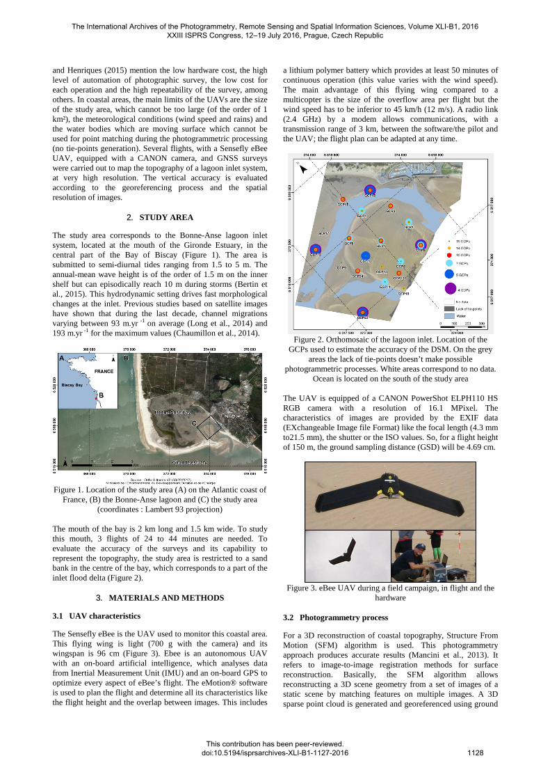
The study area corresponds to the Bonne-Anse lagoon inlet system, located at the mouth of the Gironde Estuary, in the central part of the Bay of Biscay (Figure 1). The area is submitted to semi-diurnal tides ranging from 1.5 to 5 m. The annual-mean wave height is of the order of 1.5 m on the inner shelf but can episodically reach 10 m during storms (Bertin et al., 2015). This hydrodynamic setting drives fast morphological changes at the inlet. Previous studies based on satellite images have shown that during the last decade, channel migrations varying between 93 m.yr -1 on average (Long et al., 2014) and 193 m.yr -1 for the maximum values (Chaumillon et al., 2014).

Figure 1. Location of the study area (A) on the Atlantic coast of

France, (B) the Bonne-Anse lagoon and (C) the study area (coordinates : Lambert 93 projection)

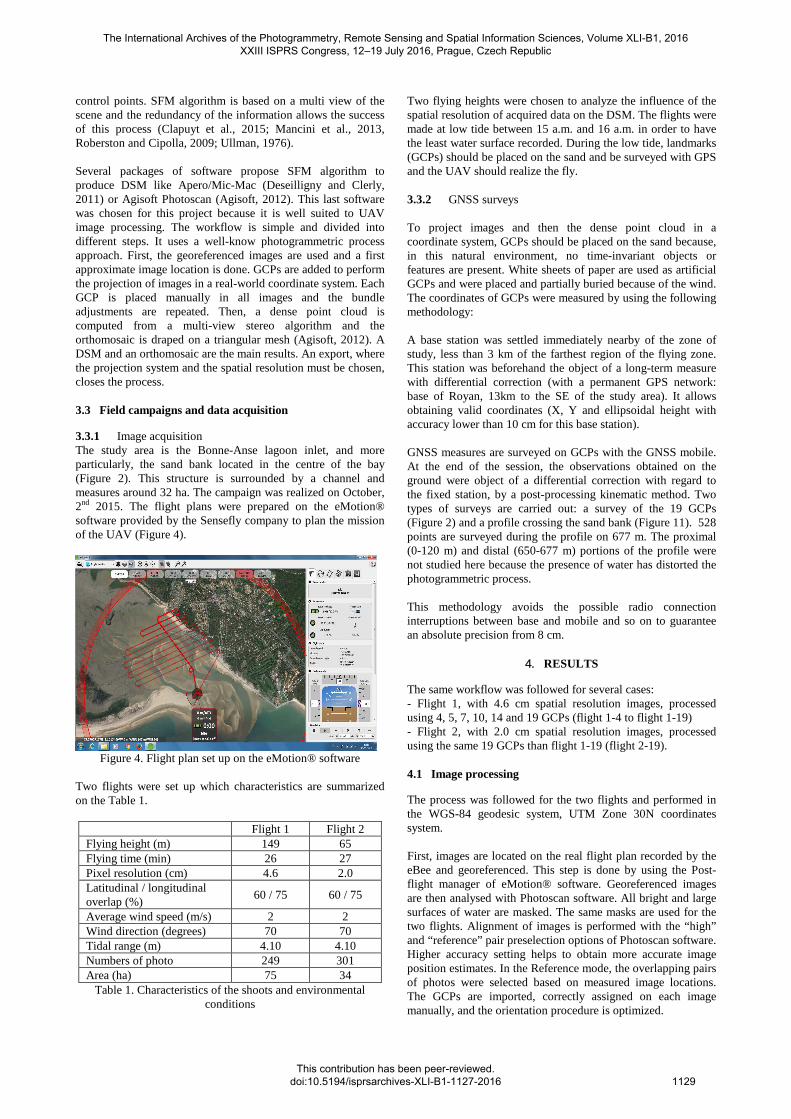
The mouth of the bay is 2 km long and 1.5 km wide. To study this mouth, 3 flights of 24 to 44 minutes are needed. To evaluate the accuracy of the surveys and its capability to represent the topography, the study area is restricted to a sand bank in the centre of the bay, which corresponds to a part of the inlet flood delta (Figure 2).

3. MATERIALS AND METHODS

3.1 UAV characteristics

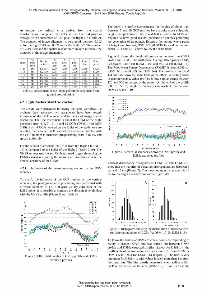
The Sensefly eBee is the UAV used to monitor this coastal area. This flying wing is light (700 g with the camera) and its wingspan is 96 cm (Figure 3). Ebee is an autonomous UAV with an on-board artificial intelligence, which analyses data from Inertial Measurement Unit (IMU) and an on-board GPS to optimize every aspect of eBee’s flight. The eMotion® software is used to plan the flight and determine all its characteristics like the flight height and the overlap between images. This includes

a lithium polymer battery which provides at least 50 minutes of continuous operation (this value varies with the wind speed). The main advantage of this flying wing compared to a multicopter is the size of the overflow area per flight but the wind speed has to be inferior to 45 km/h (12 m/s). A radio link (2.4 GHz) by a modem allows communications, with a transmission range of 3 km, between the software/the pilot and the UAV; the flight plan can be adapted at any time.

Figure 2. Orthomosaic of the lagoon inlet. Location of the

GCPs used to estimate the accuracy of the DSM. On the grey areas the lack of tie-points doesn’t make possible

photogrammetric processes. White areas correspond to no data. Ocean is located on the south of the study area

The UAV is equipped of a CANON PowerShot ELPH110 HS RGB camera with a resolution of 16.1 MPixel. The characteristics of images are provided by the EXIF data (EXchangeable Image file Format) like the focal length (4.3 mm to21.5 mm), the shutter or the ISO values. So, for a flight height of 150 m, the ground sampling distance (GSD) will be 4.69 cm.

Figure 3. eBee UAV during a field campaign, in flight and the

hardware 3.2 Photogrammetry process

For a 3D reconstruction of coastal topography, Structure From Motion (SFM) algorithm is used. This photogrammetry approach produces accurate results (Mancini et al., 2013). It refers to image-to-image registration methods for surface reconstruction. Basically, the SFM algorithm allows reconstructing a 3D scene geometry from a set of images of a static scene by matching features on multiple images. A 3D sparse point cloud is generated and georeferenced using ground



1128

control points. SFM algorithm is based on a multi view of the scene and the redundancy of the information allows the success of this process (Clapuyt et al., 2015; Mancini et al., 2013, Roberston and Cipolla, 2009; Ullman, 1976). Several packages of software propose SFM algorithm to produce DSM like Apero/Mic-Mac (Deseilligny and Clerly, 2011) or Agisoft Photoscan (Agisoft, 2012). This last software was chosen for this project because it is well suited to UAV image processing. The workflow is simple and divided into different steps. It uses a well-know photogrammetric process approach. First, the georeferenced images are used and a first approximate image location is done. GCPs are added to perform the projection of images in a real-world coordinate system. Each GCP is placed manually in all images and the bundle adjustments are repeated. Then, a dense point cloud is computed from a multi-view stereo algorithm and the orthomosaic is draped on a triangular mesh (Agisoft, 2012). A DSM and an orthomosaic are the main results. An export, where the projection system and the spatial resolution must be chosen, closes the process. 3.3 Field campaigns and data acquisition

3.3.1 Image acquisition The study area is the Bonne-Anse lagoon inlet, and more particularly, the sand bank located in the centre of the bay (Figure 2). This structure is surrounded by a channel and measures around 32 ha. The campaign was realized on October, 2nd 2015. The flight plans were prepared on the eMotion® software provided by the Sensefly company to plan the mission of the UAV (Figure 4).

Figure 4. Flight plan set up on the eMotion® software

Two flights were set up which characteristics are summarized on the Table 1.

Flight 1 Flight 2 Flying height (m) 149 65 Flying time (min) 26 27 Pixel resolution (cm) 4.6 2.0 Latitudinal / longitudinal overlap (%)

60 / 75 60 / 75

Average wind speed (m/s) 2 2 Wind direction (degrees) 70 70 Tidal range (m) 4.10 4.10 Numbers of photo 249 301 Area (ha) 75 34

Table 1. Characteristics of the shoots and environmental conditions

Two flying heights were chosen to analyze the influence of the spatial resolution of acquired data on the DSM. The flights were made at low tide between 15 a.m. and 16 a.m. in order to have the least water surface recorded. During the low tide, landmarks (GCPs) should be placed on the sand and be surveyed with GPS and the UAV should realize the fly. 3.3.2 GNSS surveys To project images and then the dense point cloud in a coordinate system, GCPs should be placed on the sand because, in this natural environment, no time-invariant objects or features are present. White sheets of paper are used as artificial GCPs and were placed and partially buried because of the wind. The coordinates of GCPs were measured by using the following methodology: A base station was settled immediately nearby of the zone of study, less than 3 km of the farthest region of the flying zone. This station was beforehand the object of a long-term measure with differential correction (with a permanent GPS network: base of Royan, 13km to the SE of the study area). It allows obtaining valid coordinates (X, Y and ellipsoidal height with accuracy lower than 10 cm for this base station). GNSS measures are surveyed on GCPs with the GNSS mobile. At the end of the session, the observations obtained on the ground were object of a differential correction with regard to the fixed station, by a post-processing kinematic method. Two types of surveys are carried out: a survey of the 19 GCPs (Figure 2) and a profile crossing the sand bank (Figure 11). 528 points are surveyed during the profile on 677 m. The proximal (0-120 m) and distal (650-677 m) portions of the profile were not studied here because the presence of water has distorted the photogrammetric process. This methodology avoids the possible radio connection interruptions between base and mobile and so on to guarantee an absolute precision from 8 cm.

4. RESULTS

The same workflow was followed for several cases: - Flight 1, with 4.6 cm spatial resolution images, processed using 4, 5, 7, 10, 14 and 19 GCPs (flight 1-4 to flight 1-19) - Flight 2, with 2.0 cm spatial resolution images, processed using the same 19 GCPs than flight 1-19 (flight 2-19). 4.1 Image processing

The process was followed for the two flights and performed in the WGS-84 geodesic system, UTM Zone 30N coordinates system. First, images are located on the real flight plan recorded by the eBee and georeferenced. This step is done by using the Post-flight manager of eMotion® software. Georeferenced images are then analysed with Photoscan software. All bright and large surfaces of water are masked. The same masks are used for the two flights. Alignment of images is performed with the “high” and “reference” pair preselection options of Photoscan software. Higher accuracy setting helps to obtain more accurate image position estimates. In the Reference mode, the overlapping pairs of photos were selected based on measured image locations. The GCPs are imported, correctly assigned on each image manually, and the orientation procedure is optimized.



1129

As results, the residual error derived from the spatial transformation, computed on GCPs, is less than 0.4 pixel in average, with a maximum of 0.53 pixel for flight 1-7 (Table 2). The accuracy of image alignment is very good, between 0.012 m for the flight 2-19 and 0.021 m for the flight 1-7. The number of GCPs used and the spatial resolution of images influence the accuracy of the image orientation.

Flight No.

photo used

No. tie points

X Error (m)

Y Error (m)

Z Error (m)

Error (m)

Error (pixel)

1 -19 249 800 597 0.016 0.016 0.016 0.016 0.323 1-14 249 802 639 0.014 0.011 0.009 0.020 0.329 1-10 249 802 835 0.010 0.007 0.007 0.014 0.316 1-7 249 802 573 0.021 0.021 0.021 0.021 0.361 1-5 249 802 370 0.009 0.011 0.004 0.014 0.283 1-4 249 802 306 0.009 0.009 0.001 0.013 0.286 2-19 301 351 977 0.012 0.012 0.012 0.012 0.141

Table 2. Assessment of the image georeferencing error from ground control points

4.2 Digital Surface Model construction

The DSMs were generated following the same workflow. To evaluate their accuracy, two parameters have been tested: influence of the GCP number and influence of image spatial resolution. The first assessment is about the DSM of the flight generated from 4, 5, 7, 10, 14 and 19 GCPs (DSM 1-4 to DSM 1-19). First, 4 GCPs located on the limits of the study area are selected, then another GCP is added on area center and to finish the GCP number is increased progressively, from 7 to 19, and spread uniformly. For the second assessment, the DSM from the flight 1 (DSM 1-19) is compared to the DSM of the flight 2 (DSM 2-19). The GNSS surveys (profile and GCPs not used to georeferencing the DSM) carried out during the mission are used to estimate the vertical accuracy of the DSMs. 4.2.1 Influence of the georeferencing method on the DSM accuracy To clarify the influence of the GCP number on the vertical accuracy, the photogrammetric processing was performed with different numbers of GCPs (Figure 2). By extraction of the DSM points, it is possible to compare the ellipsoidal height data with the GNSS profile (Figure 5 and Table 3).

Figure 5. Ellipsoidal heights of GNSS profile and DSMs

extracted profiles

The DSM 1-4 profile overestimates the heights of about 1 m. Between 5 and 19 GCP profiles have a quite close ellipsoidal height, except between 560 m and 650 m where 14 GCPs are required to have good results (presence of puddles perturbing the generation of tie-points). Except a few points where peaks of height are observed, DSM 1-7 (all GCPs focused on the sand bank), 1-14 and 1-19 curves follow the same trend. Figure 6 shows the height discrepancies between the GNSS profile and DSMs. The Arithmetic Average Discrepancy (AAD) is between 7.887 cm (DSM 1-19) and 93.773 cm (DSM 1-4). The Root Mean Square Discrepancy (RMSD) is from 9.086 cm (DSM 1-19) to 94.359 cm (DSM 1-4). The profile of the DSM 1-4 does not show the same trend as the others, reflecting errors in georeferencing. Other profiles follow similar trends between 120 and 500 m, except at the peaks. On the end of the profile (500 to 650 m) height discrepancy can reach 30 cm between DSMs 1-5 and 1-19.

Figure 6. Vertical discrepancy between GNSS profile and

DSMs extracted profiles Vertical discrepancy histograms of DSM 1-7 and DSM 1-19 show that the majority of elevation discrepancies are between 5 cm and 15 cm (Figure 7). The most common discrepancy is 10 cm for the flight 1-7 and 7 cm for the flight 1-19.

Figure 7. Histograms showing the distribution of discrepancies for different numbers of GCPs (A: DSM 1-7; B: DSM 1-19)

To know the ability of DSMs to create points corresponding to reality, a scatter (XYZ) plot was carried out between GNSS profile and DSMs extracted profiles. Except for DSM 1-4, the coefficients of determination (R²) are close to 1: from 0.958 for DSM 1-5 to 0.973 for DSM 1-14 (Figure 8). The bias is very important for DSM 1-4, with values located more than 1 m from the trend line. The bias greatly decreased when adding a fifth GCP in the center of the area (DSM 1-5). If we increase the



1130

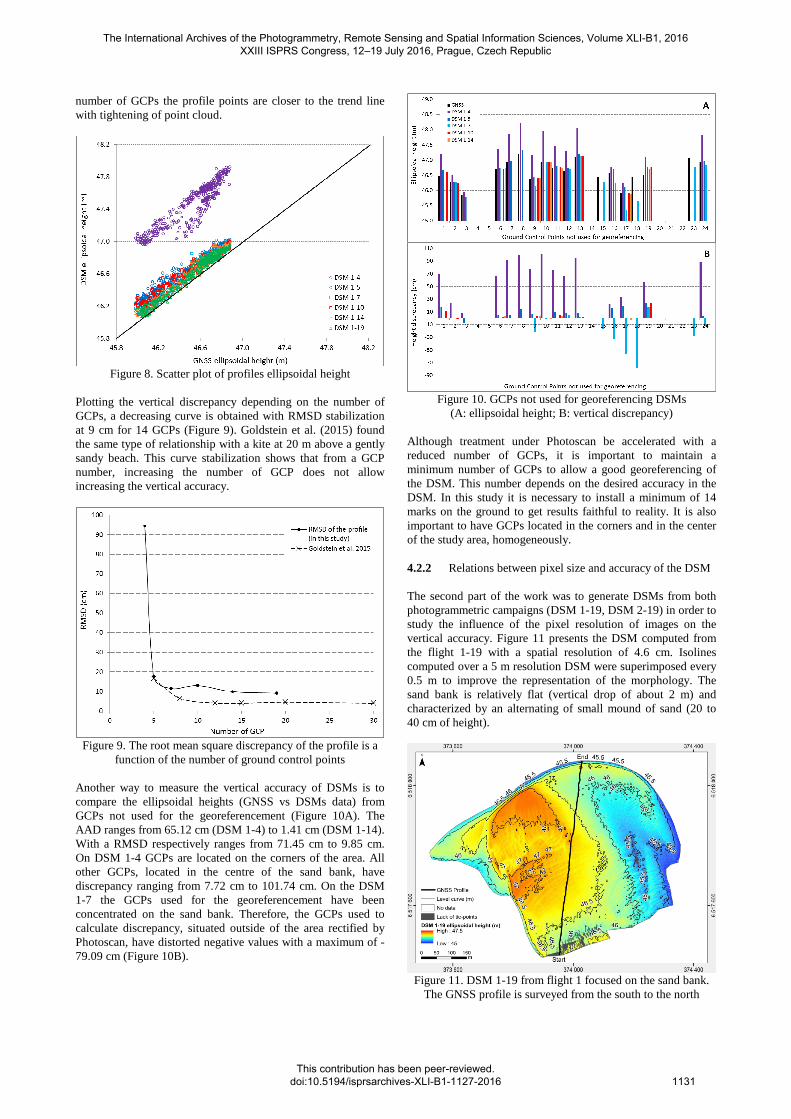
number of GCPs the profile points are closer to the trend line with tightening of point cloud.

Figure 8. Scatter plot of profiles ellipsoidal height

Plotting the vertical discrepancy depending on the number of GCPs, a decreasing curve is obtained with RMSD stabilization at 9 cm for 14 GCPs (Figure 9). Goldstein et al. (2015) found the same type of relationship with a kite at 20 m above a gently sandy beach. This curve stabilization shows that from a GCP number, increasing the number of GCP does not allow increasing the vertical accuracy.

Figure 9. The root mean square discrepancy of the profile is a

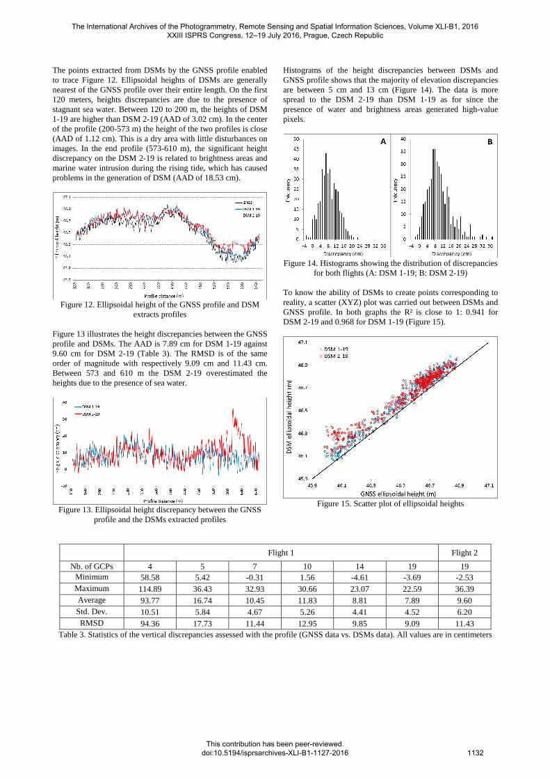
function of the number of ground control points Another way to measure the vertical accuracy of DSMs is to compare the ellipsoidal heights (GNSS vs DSMs data) from GCPs not used for the georeferencement (Figure 10A). The AAD ranges from 65.12 cm (DSM 1-4) to 1.41 cm (DSM 1-14). With a RMSD respectively ranges from 71.45 cm to 9.85 cm. On DSM 1-4 GCPs are located on the corners of the area. All other GCPs, located in the centre of the sand bank, have discrepancy ranging from 7.72 cm to 101.74 cm. On the DSM 1-7 the GCPs used for the georeferencement have been concentrated on the sand bank. Therefore, the GCPs used to calculate discrepancy, situated outside of the area rectified by Photoscan, have distorted negative values with a maximum of -79.09 cm (Figure 10B).

Figure 10. GCPs not used for georeferencing DSMs

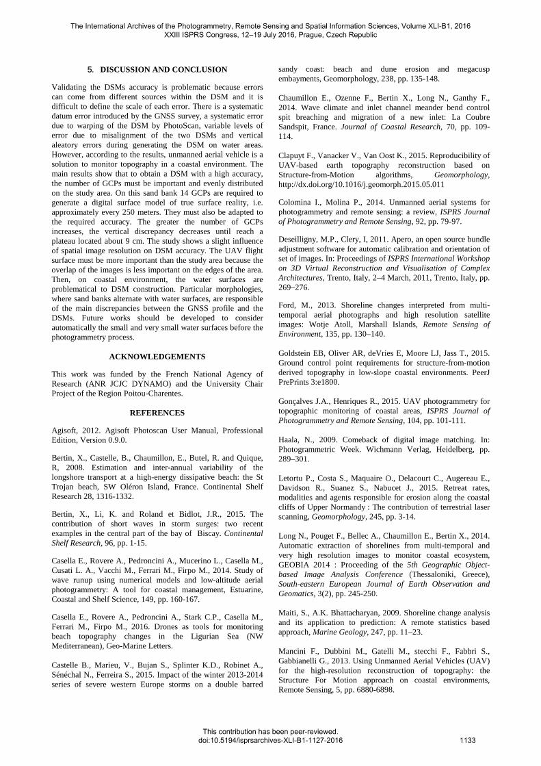
(A: ellipsoidal height; B: vertical discrepancy) Although treatment under Photoscan be accelerated with a reduced number of GCPs, it is important to maintain a minimum number of GCPs to allow a good georeferencing of the DSM. This number depends on the desired accuracy in the DSM. In this study it is necessary to install a minimum of 14 marks on the ground to get results faithful to reality. It is also important to have GCPs located in the corners and in the center of the study area, homogeneously. 4.2.2 Relations between pixel size and accuracy of the DSM The second part of the work was to generate DSMs from both photogrammetric campaigns (DSM 1-19, DSM 2-19) in order to study the influence of the pixel resolution of images on the vertical accuracy. Figure 11 presents the DSM computed from the flight 1-19 with a spatial resolution of 4.6 cm. Isolines computed over a 5 m resolution DSM were superimposed every 0.5 m to improve the representation of the morphology. The sand bank is relatively flat (vertical drop of about 2 m) and characterized by an alternating of small mound of sand (20 to 40 cm of height).

Figure 11. DSM 1-19 from flight 1 focused on the sand bank.

The GNSS profile is surveyed from the south to the north



1131

The points extracted from DSMs by the GNSS profile enabled to trace Figure 12. Ellipsoidal heights of DSMs are generally nearest of the GNSS profile over their entire length. On the first 120 meters, heights discrepancies are due to the presence of stagnant sea water. Between 120 to 200 m, the heights of DSM 1-19 are higher than DSM 2-19 (AAD of 3.02 cm). In the center of the profile (200-573 m) the height of the two profiles is close (AAD of 1.12 cm). This is a dry area with little disturbances on images. In the end profile (573-610 m), the significant height discrepancy on the DSM 2-19 is related to brightness areas and marine water intrusion during the rising tide, which has caused problems in the generation of DSM (AAD of 18.53 cm).

Figure 12. Ellipsoidal height of the GNSS profile and DSM

extracts profiles Figure 13 illustrates the height discrepancies between the GNSS profile and DSMs. The AAD is 7.89 cm for DSM 1-19 against 9.60 cm for DSM 2-19 (Table 3). The RMSD is of the same order of magnitude with respectively 9.09 cm and 11.43 cm. Between 573 and 610 m the DSM 2-19 overestimated the heights due to the presence of sea water.

Figure 13. Ellipsoidal height discrepancy between the GNSS

profile and the DSMs extracted profiles

Histograms of the height discrepancies between DSMs and GNSS profile shows that the majority of elevation discrepancies are between 5 cm and 13 cm (Figure 14). The data is more spread to the DSM 2-19 than DSM 1-19 as for since the presence of water and brightness areas generated high-value pixels.

Figure 14. Histograms showing the distribution of discrepancies

for both flights (A: DSM 1-19; B: DSM 2-19) To know the ability of DSMs to create points corresponding to reality, a scatter (XYZ) plot was carried out between DSMs and GNSS profile. In both graphs the R² is close to 1: 0.941 for DSM 2-19 and 0.968 for DSM 1-19 (Figure 15).

Figure 15. Scatter plot of ellipsoidal heights

Flight 1 Flight 2

Nb. of GCPs 4 5 7 10 14 19 19 Minimum 58.58 5.42 -0.31 1.56 -4.61 -3.69 -2.53 Maximum 114.89 36.43 32.93 30.66 23.07 22.59 36.39 Average 93.77 16.74 10.45 11.83 8.81 7.89 9.60 Std. Dev. 10.51 5.84 4.67 5.26 4.41 4.52 6.20 RMSD 94.36 17.73 11.44 12.95 9.85 9.09 11.43

Table 3. Statistics of the vertical discrepancies assessed with the profile (GNSS data vs. DSMs data). All values are in centimeters



1132

5. DISCUSSION AND CONCLUSION

Validating the DSMs accuracy is problematic because errors can come from different sources within the DSM and it is difficult to define the scale of each error. There is a systematic datum error introduced by the GNSS survey, a systematic error due to warping of the DSM by PhotoScan, variable levels of error due to misalignment of the two DSMs and vertical aleatory errors during generating the DSM on water areas. However, according to the results, unmanned aerial vehicle is a solution to monitor topography in a coastal environment. The main results show that to obtain a DSM with a high accuracy, the number of GCPs must be important and evenly distributed on the study area. On this sand bank 14 GCPs are required to generate a digital surface model of true surface reality, i.e. approximately every 250 meters. They must also be adapted to the required accuracy. The greater the number of GCPs increases, the vertical discrepancy decreases until reach a plateau located about 9 cm. The study shows a slight influence of spatial image resolution on DSM accuracy. The UAV flight surface must be more important than the study area because the overlap of the images is less important on the edges of the area. Then, on coastal environment, the water surfaces are problematical to DSM construction. Particular morphologies, where sand banks alternate with water surfaces, are responsible of the main discrepancies between the GNSS profile and the DSMs. Future works should be developed to consider automatically the small and very small water surfaces before the photogrammetry process.

ACKNOWLEDGEMENTS

This work was funded by the French National Agency of Research (ANR JCJC DYNAMO) and the University Chair Project of the Region Poitou-Charentes.

REFERENCES

Agisoft, 2012. Agisoft Photoscan User Manual, Professional Edition, Version 0.9.0.

Bertin, X., Castelle, B., Chaumillon, E., Butel, R. and Quique, R, 2008. Estimation and inter-annual variability of the longshore transport at a high-energy dissipative beach: the St Trojan beach, SW Oléron Island, France. Continental Shelf Research 28, 1316-1332.

Bertin, X., Li, K. and Roland et Bidlot, J.R., 2015. The contribution of short waves in storm surges: two recent examples in the central part of the bay of Biscay. Continental Shelf Research, 96, pp. 1-15.

Casella E., Rovere A., Pedroncini A., Mucerino L., Casella M., Cusati L. A., Vacchi M., Ferrari M., Firpo M., 2014. Study of wave runup using numerical models and low-altitude aerial photogrammetry: A tool for coastal management, Estuarine, Coastal and Shelf Science, 149, pp. 160-167.

Casella E., Rovere A., Pedroncini A., Stark C.P., Casella M., Ferrari M., Firpo M., 2016. Drones as tools for monitoring beach topography changes in the Ligurian Sea (NW Mediterranean), Geo-Marine Letters. Castelle B., Marieu, V., Bujan S., Splinter K.D., Robinet A., Sénéchal N., Ferreira S., 2015. Impact of the winter 2013-2014 series of severe western Europe storms on a double barred

sandy coast: beach and dune erosion and megacusp embayments, Geomorphology, 238, pp. 135-148. Chaumillon E., Ozenne F., Bertin X., Long N., Ganthy F., 2014. Wave climate and inlet channel meander bend control spit breaching and migration of a new inlet: La Coubre Sandspit, France. Journal of Coastal Research, 70, pp. 109-114. Clapuyt F., Vanacker V., Van Oost K., 2015. Reproducibility of UAV-based earth topography reconstruction based on Structure-from-Motion algorithms, Geomorphology, http://dx.doi.org/10.1016/j.geomorph.2015.05.011

Colomina I., Molina P., 2014. Unmanned aerial systems for photogrammetry and remote sensing: a review, ISPRS Journal of Photogrammetry and Remote Sensing, 92, pp. 79-97.

Deseilligny, M.P., Clery, I, 2011. Apero, an open source bundle adjustment software for automatic calibration and orientation of set of images. In: Proceedings of ISPRS International Workshop on 3D Virtual Reconstruction and Visualisation of Complex Architectures, Trento, Italy, 2–4 March, 2011, Trento, Italy, pp. 269–276.

Ford, M., 2013. Shoreline changes interpreted from multi-temporal aerial photographs and high resolution satellite images: Wotje Atoll, Marshall Islands, Remote Sensing of Environment, 135, pp. 130–140. Goldstein EB, Oliver AR, deVries E, Moore LJ, Jass T., 2015. Ground control point requirements for structure-from-motion derived topography in low-slope coastal environments. PeerJ PrePrints 3:e1800. Gonçalves J.A., Henriques R., 2015. UAV photogrammetry for topographic monitoring of coastal areas, ISPRS Journal of Photogrammetry and Remote Sensing, 104, pp. 101-111. Haala, N., 2009. Comeback of digital image matching. In: Photogrammetric Week. Wichmann Verlag, Heidelberg, pp. 289–301. Letortu P., Costa S., Maquaire O., Delacourt C., Augereau E., Davidson R., Suanez S., Nabucet J., 2015. Retreat rates, modalities and agents responsible for erosion along the coastal cliffs of Upper Normandy : The contribution of terrestrial laser scanning, Geomorphology, 245, pp. 3-14. Long N., Pouget F., Bellec A., Chaumillon E., Bertin X., 2014. Automatic extraction of shorelines from multi-temporal and very high resolution images to monitor coastal ecosystem, GEOBIA 2014 : Proceeding of the 5th Geographic Object-based Image Analysis Conference (Thessaloniki, Greece), South-eastern European Journal of Earth Observation and Geomatics, 3(2), pp. 245-250. Maiti, S., A.K. Bhattacharyan, 2009. Shoreline change analysis and its application to prediction: A remote statistics based approach, Marine Geology, 247, pp. 11–23. Mancini F., Dubbini M., Gatelli M., stecchi F., Fabbri S., Gabbianelli G., 2013. Using Unmanned Aerial Vehicles (UAV) for the high-resolution reconstruction of topography: the Structure For Motion approach on coastal environments, Remote Sensing, 5, pp. 6880-6898.



1133

Nagihara S., Kevin R., Mulligan R. Xiong W., 2004. Use of the tree-dimensional laser scanner to digitally capture the topography of sand dunes in high spatial resolution, Earth Surface Processes and Landforms, 29, pp. 391-398. Pardo-Pascual, J.E., J. Almonacid-Caballer, L.A. Ruiz, J. Palomar-Vazquez, 2012. Automatic extraction of shorelines from Landsat TM and ETM+ multi-temporal images with subpixel precision, Remote sensing of Environment, 123, pp 1–11. Quartel, S., E.A. Addink, B.G. Ruessink, 2006. Object-oriented extraction of beach morphology from video images, International Journal of applied Earth Observation and Geoinformation, 8, pp. 256-269.

Robertson D.P. and Cipolla R., 2009. Structure from Motion, in Varga M. editors, Practical image processing and computer vision, John Wiley, chapter 13, 24p.

Ryu, J.H., Won, J.S., Min, K.D., 2002. Waterline extraction from Landsat TM data in a tidal flat: A case study in Gomso Bay, Korea, Remote Sensing of Environment, 83, pp. 442–456.

Taveira-Pinto, F., Silva, R., Barbosa, J., 2011. Coastal erosion along the Portuguese northwest coast due to changing sediment discharges from rivers and climate change. In: Schernewski, G., Hofstede, J., Neumann, T. (Eds.), Global Change and Baltic Coastal Zones, Vol. 1. Coastal Research Library, Springer, pp. 135–151.

Thieler E.R., W.W. Danforth, 1994. Historical Shoreline Mapping (I): Improving Techniques and Reducing Positioning Errors, Journal of Coastal Research, 10 (3), pp. 549–563.

Ullman S., 1979. The interpretation of structure from motion, Proceedings of the Royal Society of London, 203, 1153, 35p

White S. A., Wang Y., 2003. Utilizing DEMs derived from LIDAR data to analyze morphologic change in the North Carolina coastline, Remote Sensing of Environment, 85, pp39-47.



1134

accuracy assessment of coastal topography derived from uav

Documents