accuracy standards of tying the horizontal and...

GEOMATICS AND ENVIRONMENTAL ENGINEERING • Volume 8 • Number 3 • 2014

http://dx.doi.org/10.7494/geom.2014.8.3.41

41

Janusz Dąbrowski*

Accuracy Standards of Tying the Horizontal and Vertical Control Network

to the National Geodetic Control Network

1. Introduction

To adjust the survey results of multi‑row networks the Gauss–Markov model can be used, including accuracy weight matrix for the values observed, as well as in‑cluding the apparent observational equations for the coordinates of tie points. To the apparent observational equations the relevant accuracy weights are assigned for the analysed coordinate points or their covariance matrices. Many authors of scientific papers use for that purpose the sequential adjustment of measurement results, i.e. the adjustment carried out in a few stages. By foreign authors, there are the works of Baardy [2], Teunissen [14] and Rao [13]. By domestic authors, there are the pa‑pers of Adamczewski [1], Baran [3], Gaździcki [7], Kadaj [8], Wiśniewski [15] and Kamiński [9]. Many computer programmes, e.g. GOENET [8], use this procedure to adjust measurement results of the multirow control networks.

The issue of the estimation of the horizontal and vertical control point coordi‑nates in tying to national geodetic control networks is similar to multirow networks adjustment but specific allocation of these networks set down different conditions of tying them to national geodetic control networks. This problem, in relation to determination of point displacement, was worked on in Canada by Chrzanowski [4] and in Germany by Pelzer [10]. Similar deliberations were made nationally by Cza‑ja [6] and Prószyński and Kwaśniak [12]. The deliberations included in this pub‑lication will only be referred to three thematically nearest positions, i.e. Czaja [5], Prószyński [11] and Wiśniewski [16]. In paper [5] the author proposes to include the observations of connecting national geodetic control network points to the adjuste‑ment of horizontal and vertical control network. For the coordinates of national ge‑odetic control points the author proposes to juxtapose the pseudo‑observation equa‑tions including their ccovariance matrices. Prószyński [11] in his paper presents the method of tying the horizontal and vertical control networks to the national geodetic

* AGH University of Science and Technology, Faculty of Mining Surveying and Environmental Engi‑neering, Department of Geomatics, Krakow, Poland

42 J. Dąbrowski

control networks with use of Helmert transformation parameters. In the first stage, the horizontal and vertical control network, along with selected points of national geodetic control network, is freely adjusted in local system. In the second stage, the local system is transformed into national system, on the basis of previously estimat‑ed transformation parameters for adjustment points, namely turn and displacement. Wiśniewski [16] in his paper deals with observation results adjustment in geodetic networks. Deliberations included in Chapter 6 refer to the adjustment of results with the use of sequential method, i.e. carried out for different stages of geodetic network measurement. The gist of this method is to include in each stage the adjustment of results obtained in previous stages. Wiśniewski [16] proved that the formulated pseudo‑observation equations for the point coordinates and their covariance matri‑ces, obtained in the preceding stages, have identical estimates to the adjustment of the whole geodetic network in one stage.

Horizontal and vertical control networks are used for marking out structures in the field, therefore the coordinates of their points have to be marked with high accuracy. The accuracy of horizontal and vertical control networks is at least by one range higher than the one of national geodetic control networks. Tying the hori‑zontal and vertical control networks to the coordinates of national geodetic con‑trol points is done by means of geodetic tie construction. Tie construction consists of a selected group of horizontal and vertical control network points and national geodetic control network points, in which the angles and lenghts marked by these points are measured.

The adjustment of measurement results in tie construction leads to determina‑tion of coordinate estimates of the selected horizontal and vertical control points and the national geodetic control points as well as their covariance matrices. For the estimation of point coordinates in tie construction covariance matrix must be used for the coordinates of selected national geodetic control network points.

Final adjustment of measurement results in the horizontal and vertical control network cannot be affected by inaccuracy of the national geodetic control point co‑ordinates, included in tie construction.

To formulate the accuracy criteria for tying horizontal and vertical control net‑work it is necessary, for tie construction, to introduce separate formulas for estima‑tion of point coordinates and their covariance matrices of the horizontal and verti‑cal control network and the national geodetic control network. The introduction of these formulas is done by way of solving the system of four matrix equations, which result from the reciprocal of properly defined block matrix.

The criterion for the proper way of tying the horizontal and vertical control network is assumed as the relation of standard deviation value for the intervals between points in tie construction to the medium standard deviation of the sides lenght measurement in this construction. Value of the standard deviation is deter‑mined on the basis of the variance coefficient obtained from the estimation of points coordinates in tie construction and the variance included in the weight matrix for

Accuracy Standards of Tying the Horizontal and Vertical Control Network... 43

the measured lenghts. On the basis of this relation, three methods of tying horizontal and vertical control networks to the national coordinate system have been proposed.

The proposed methods of tying the horizontal and vertical control network can be used in marking out the structures in small areas as well as to mark out border markers of the residential plots in the field.

The practical application of the proposed algorithm for the determination of proper method of tying the horizontal and vertical control network, along with the interpretation of calculations results, is illustrated in the final part of this thesis in the form of numerical example.

2. Theoretical Foundations of Gauss–Markov Model (L, AX, G) with Random Parameters

It is assumed that L is a vector of the observed random variables, the mean val‑ue of which can be descibed with the use of the established linear AX models, where X represents the vector of the estimated parameters, and A represents the matrix of known coefficients in estimated parameters. In geodetic networks the values of these coefficients are the partial derivatives values of the observed elements (angles and lenghts) in relation to coordinates of points that specify these elements. The estimate parameters, on the other hand, are coordinate differentials of the national gedetic control points of tying and coordinate differentials of the horizontal and vertical control networks which are subject to connection.

It is assumed that the vector of estimated parameters X is also a random variable with covariance matrix C.

To the observed values the condition is applied that matrix G is a condition‑al covariance matrix of the observations L with established parameters X, namely

( )= \VH L X .Considering the above assumptions, the conditional covariance matrix of the

observations L is determined according to the dependancy [13]:

= + = + = +( ) [ ( )] ( ( ) ( ) TV E V V E VL L \ X L \ X G AX G ACA (1)

In order to divide the process of differentials estimation to the horizontal and vertical control points coordinates to the process of differentials estimation of na‑tional geodetic control network points coordinates, with established covariance ma‑trix C, the coefficients matrix A has to be divided into two parts, namely matrices A1 and A2. Matrix A1 represents the coefficients of the national geodetic control point coordinates differentials, while A2 matrix represents the horizontal and vertical con‑trol points coordinates differentials. Simultaneously the estimated parameters X are subject to the analogical division into X1 and X2.

44 J. Dąbrowski

Considering the above notations, the observational equations for the tie con‑struction can be presented in the following block matrices formula:

× =

11 2

2

XA A LXI 0 0

(2)

For the equations (2) covariance matrix is defined in form of the following block matrix:

=

1cov( ; )G 0

L X0 C

(3)

where: G – a conditional covariance matrix of observations L with established

parameters, C – a covariance matrix for multidimensional random variable that rep‑

resents coordinates of the national geodetic control network points.

After carrying out the principle of the smallest quare sum of random deviations for the system (2), including covariance matrix (3), the normal equations system is presented in form of block matrices [6, 16]:

− − − − −

− − −

+× = ×

1 1 1 1 111 1 1 2 1

1 1 122 1 2 2 2

T T T

T T T

X LA G A C A G A A G CX 0A G A A G A A G 0

(4)

In order to solve the normal equations system (4), with the division of estimat‑ed parameters into differentials vectors X1 and X2, it is necessary to determine the reciprocal of the block matrix that exists in the product with these parameters. To simply the analitical conversion for the block matrix elements the following notation is assumed:

− − −

− −

+=

1 1 11 121 1 2

1 112 22 1 2 2

T T

TT T1 N NA G A C A G A

N NA G A A G A (5)

The reciprocal of block matrix (5) is defined with use of the following condition:

× =

1 12 1 12

12 2 12 2T T

N N H H I 0N N H H 0 I

(6)


Realisation of the condition (6) leads to four matrix equations system in the following form:

+ =+ =

+ =

+ =

1 1 12 12

1 12 12 2

12 1 2 12

12 12 2 2

T

T T

T

N H N H IN H N H 0N H N H 0N H N H I

(7)

Solving the above equation system leads to the following matrix formula H1, H2 and H12:

− −= − 1 11 1 12 2 12( )TH N N N N (8)

− −= − 1 12 2 12 1 12( )TH N N N N (9)

1 1 112 1 12 2 12 1 12( )T− − −= − × −H N N N N N N (10)

On the basis of formulas (8), (9) and (10) for the reciprocal of block matrix (6), solution of the equation system (4) can be written in the following explicit form:

− −

−

= × ×

1 11 1 12 1

112 2 22

ˆ

ˆ

T

T T

X H H LA G CH H 0A G 0X

(11)

The derived formula (11) enables to estimate seperately the differentials to na‑tional geodetic control points coordinates, in form of vector 1X̂ , and the differentials to approximate coordinates of the horizontal and vertical control points, in form of vector 2X̂ .

After realization of proper matrix products in the formula (11) for the first row of block matrix H, vector 1X̂ is expressed by the following dependence:

− −= + ×1 11 1 1 12 2

ˆ ( )T TX H A G H A G L (12)

Replacing the above dependence by the formula (8) and extracting matrix H1 from brackets we get final formula for estimated differentials to national geodetic control points coordinates, which is:

− − −= − ×1 1 11 1 1 12 2 2

ˆ ( )T TX H A G N N A G L (13)

46 J. Dąbrowski

After getting matrix product (11) for the second row of matrix H and after per‑forming similar transformations like in formula (13), vector X2 is determined by the following relation:

− − −= − ×1 1 12 2 2 12 1 1

ˆ ( )T T TX H A G N N A G L (14)

On account of the fact that the coordinates of national geodetic control points, included in the process of tying, are never corrected with the estimated differen‑tials in form of vector 1X̂ , therefore their values will be only used for estimation of random deviations for values observed in the tie construction. If the estimated differentials to the approximate coordinates of horizontal and vertical control net‑work points, represented by vector 2X̂ , are added to the approximate coordinates of points, established at the stage of just aposing the observational equations, we get the most probable coordinates of those points in the national system.

A very important problem in the presented process of estimation is the inaccu‑racy evaluation of vector 2X̂ . Variance of vector 2X̂ can be written in form of a general definition in the following form [13]:

2 2 2 2 2ˆ ˆ ˆ ˆ ˆ( ) {[ ( )] [ ( )] }TV E E E= − × −X X X X X (15)

After inserting to the above dependence the formula for vector estimate, the variance of this estimate is expressed by the relation:

− − − − − −

=

= − × − × − × −1 1 1 1 1 12 2 12 1 1 2 2 2 12 1 1 2

ˆ( ){[ ) ] [ ( ) ] }T T T T T T T

VEX

H (A G N N A G L X H A G N N A G L X (16)

If the vector of absolute terms L is replaced by the expression containing the matrices from the process of estimation as a sum of model values of the observed quantities ( 2 2

ˆA X ) and random deviations δ , namely = +2 2ˆ( )L A X δ , then after per‑

forming several transformations, the relation (16) will take the following form:

− −= = σ −2 1 12 2 0 2 12 1 12

ˆ ˆ ˆ( ) cov( ) )TV X X (N N N N (17)

when 20δ̂ states for coefficient of variance obtained in the process of vector estimation

1X̂ and 2X̂ .Random deviations vector δ to the estimated linear model (2) is a difference of

the observed random variables L and its mean value = +1 1 2 2( ˆ ˆ)E L A X A X , namely:

= −

11 2

2

ˆˆ

ˆX

L A AX

δ (18)


Thus variation coefficient in the estimated model of the tie construction is expressed by the formula:

−

σ =−

120

ˆ ˆˆ

T

n kGδ δ (19)

in which n states for the number of observed geodetic elements in the tie construc‑tion, and k is a number of estimated coordinates of horizontal and vertical control network points, which are included in the tie construction.

3. The Criteria of Tying Horizontal and Vertical Control Networks

Matrix G represented the variance matrix of the observed values (angles and lenghts) in the geodetic tie construction; therefore it will contain on the main diago‑nal only the squares of mean measurement errors. Values of those errors are estab‑lished on the basis of accuracy classes of the instruments used for measuring lenghts and angles in the tie construction. Matrix G can be written in the following form:

21

2

21

2

0 0 0 0 00 .... 0 0 0 00 0 0 0 00 0 0 0 00 0 0 0 .... 00 0 0 0 0

d

di

i

β

β

σ σ =

σ σ

G (20)

In practical solutions the mean errors for lenght measurements are accepted at equal level dσ and for angle measurement at equal level βσ .

Matrix C will be represented by covariance matrix for the coordinates of se‑lected national geodetic control network points, included in the tie construction. Matrix C should come from national geodetic control network adjustment; therefore it should have the following form:

σ

− σ −

= −

− − − − σ − − − − − σ

21 1 1 1 1

21 1 1

2

2

( )( )

(

cov( , ) cov( , ) cov( , )/ / cov( , ) cov( , )/ // // / / / / / / / cov( , )/ / / / / / / / /

))/ (

m m

m m

m m m

m

x x y x x x yy y x y y

x x yy

C (21)

48 J. Dąbrowski

If the coordinates of national geodetic control network points do not have full covariance matrix, then matrix C should contain only the elements on the main di‑agonal, the values of which should correspond to the squares of mean errors of es‑tablishing coordinates of these points.

Matrices A1 and A2 are partial derivative values of the observed elements in the tie construction calculated against the coordinates of points included in this construction.

On the basis of formulas (13) and (14) vector of unknowns is estimated, which contains differentials ,i idx dy to the coordinates of national geodetic control points as well as differentials ,i idx dy to the approximate coordinates of the horizontal and vertical control points.

According to the existing geodetic intructions, the following accuracy criteria can be mentioned. The 3rd class national geodetic control networks have specified ac‑curacy charactersitics in form of mean error of point location 2 2 10 cmP x yσ = σ + σ ≤ .

Accuracy of horizontal and vertical control network is formulated with the use of side lenght error, after final adjustment of observation resulst in this control net‑work. Value of this error, depending on an established accuracy of marking out points in the field, cannot be larger than 5 cm [5].

To formulate the criteria of tying horizontal and vertical control networks to na‑tional geodetic control networks the following estimates determined from model (2) will be used: covariance matrix ˆcov( )2X for the coordinates of horizontal and vertical control points established according to the formula (17), and variance coefficient 2

0σ̂ for the values observed in the tie construction specified with relation (19).

On the basis of the above parameters values, three ways of final coordinates estimations of horizontal and vertical control points can be formulated.

The criteria describing the way of this estimation will be defined with the fol‑lowing parameters:

– maximum value of standard deviation maxˆ( )idσ for any distance di between

the points of horizontal and vertical control network, calculated on the basis of matrix ˆcov( )2X ;

– variance coefficient 20σ̂ for the values observed in the tie construction;

– mean error dσ for length measurement assumed in the matrix G; – quantil of Student’s t‑distribution tα for ( 1)n− degrees of freedom and

(1 ) 0.95−α = significance level, which takes the following values:

n − k 1 2 3 4 5 6 7 ... 10 20 30 ... 100

tα 12.7 4.3 3.2 2.8 2.6 2.4 2.4 ... 2.2 2.1 2.0 ... 2.0


I. When standard deviations for any distance di between the points of horizon‑tal and vertical control network, filfill the inequality:

maxˆ ˆ( )i dd tασ ≤ ⋅σ ⋅σ (22)

then in the final estimation of coordinates of horizontal and vertical control points all elements of the tie construction should be included.

II. If for any distance di between the horizontal and vertical control points the inequality takes place:

maxˆˆ ˆ( ) 3d i dt d tα α⋅σ ⋅σ < σ ≤ ⋅ ⋅σ ⋅σ (23)

then the observations of the tie construction should not be included into the final coordinates estimation of the horizontal and vertical control points. In such case, in the final adjustment of the horizontal and vertical control network the estimated coordinates ˆ

2X should be considered as well as their matrix ˆcov( )2X .III. If for any distance di between the horizontal and vertical control points the

inequality takes place:

maxˆ ˆ( ) 3i dd tασ > ⋅ ⋅σ ⋅σ (24)

it means that the value of standard deviation of the distances between the horizontal and vertical control points exceeds triple value of parameters estimation inaccuracy in the model of the tie construction. In such case, tying the horizontal and vertical control network to the national coordinate system should be performed on the basis of estimated coordinates for one point of the national geodetic control network and for one point of the horizontal and vertical control network. Such tying of horizontal and vertical control network will be free of any distortions of measurement results of this control network resulting from high inaccuracy of marking out the national geodetic control network.

4. Numerical Example

To establish the way of tying the horizontal and vertical control network, which is represented by one point no. 3, the tie construction to the national geodetic con‑trol network has been analysed, represented by point no. 1 and no. 2. The elements which are subject to measurement in the tie construction are illustrated in Figure 1, while the observed values of these elements and coordinates of national geodetic control network points, reduced to point no. 1, are presented in Table 1.

50 J. Dąbrowski

Table 1. Listing of observation results of the elements in the tie construction

National geodetic control network points Measured lenghts Measured angles

point number X [m] Y [m] denotation [m] denotation [g]

1 0 0 d13 370.674 β1 52.4480

2 400.000 0 d23 309.749 β2 68.2358

3 – – – – β3 79.3172

On the basis of the observed elements, that is length d13 and angle β1 as well as the coordinates of the national geodetic control points, the approximate coordinates of point no. 3 have been calculated, that is:

( )( )

= + ⋅ β =

= + ⋅ β =3 1 13 1

3 1 13 1

cos 251.836 [m],

sin 271.989 [m].

x x d

y y d

Values of approximate coordinates of point no. 3 and the coordinates of national geodetic control points no. 1 and no. 2 are the basis for calculating the approximate values of the measured values in the tie construction, namely:

– for sides length:

( ) ( )2 2

23 3 2 3 2 6309.726d x x y y= − + − = [m],

( ) ( )2 2

13 3 1 3 1 2370.674d x x y y= − + − = [m],

Fig. 1. Tie construction outline of the horizontal and vertical control network


– for angles:

( ) ( ) ( ) ( )+ −β = ⇒ β =

⋅ ⋅

2 22

13 12 23 g1 1

13 12

cos 52.4480 [ ],2

d d d

d d

( ) ( ) ( ) ( )+ −β = ⇒ β =

⋅ ⋅

2 22

12 23 13 g2 2

23 12

cos 68.2455 [ ],2

Od d d

d d

( ) ( ) ( ) ( )+ −β = ⇒ β =

⋅ ⋅

2 2 2

23 13 12 g3 3

23 13

cos 79.3066 [ ].2

d d d

d d

On the basis of the above values the observational equations system was formu‑lated, illustrated in Table 2.

Table 2. Observation equations for the tie construction of the setting out network

Denotation of the

elementdx1 dy1 dx2 dy2 3dx 3dy Calculation of the

constant termsConstant

terms

d13 –0.679 –0.734 0 0 0.679 0.734 370.674 – 370.674 0 [mm]

d23 0 0 0.478 –0.878 –0.478 0.878 309.749 – 309.727 22 [mm]

β1 1.260 0.425 0 –1.592 –1.260 1.167 52.4480 – 52.4480 0 [cc]

β2 0 –1.592 –1.805 0.609 1.805 0.983 68.2358 – 68.2455 −97 [cc]

β3 –1.260 1.167 1.805 0.983 –0.545 –2.150 79.3172 – 79.3066 106 [cc]

A1 A2 L

In the composed system of observational equations the matrices A1, A2 and L have been marked in relevant frames.

To determine matrix G it was assumed that the measurement is carried out with the electronic tachymeter, which according to the accuracy metrics provided

5 mmdσ = and cc10βσ = . Matrix G will therefore contain the following elements:

25 0 0 0 00 25 0 0 00 0 100 0 00 0 0 100 00 0 0 0 100

=

G [mm2 ∪ cc2].

52 J. Dąbrowski

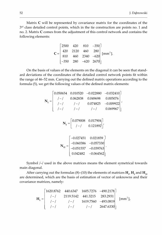
Matrix C will be represented by covariance matrix for the coordinates of the 3rd class detailed control points, which in the tie construction are points no. 1 and no. 2. Matrix C comes from the adjustment of this control network and contains the following elements:

2

2500 420 810 350420 2120 460 280

[mm ]810 460 2340 620350 280 620 2670

− = − − −

C .

On the basis of values of the elements on the diagonal it can be seen that stand‑ard deviations of the coordinates of the detailed control network points fit within the range of 46–52 mm. Carrying out the defined matrix operations according to the formula (5), we get the following values of the defined matrix elements:

0.050654 0.010520 0.022880 0.032410/ / 0.062838 0.049698 0.005076/ / / / 0.074825 0.009922/ / / / / / 0.069967

− − − = − − −

− − −

1N ,

0.079008 0.017904

/ / 0.121892

= − 2N ,

0.027451 0.0218590.060386 0.0573300.051557 0.039763

0.042482 0.064562

− − − = − −

−

12N .

Symbol /–/ used in the above matrices means the element symetrical towards main diagonal.

After carrying out the formulas (8)–(10) the elements of matrices H1, H2 and H12 are determined, which are the basis of estimation of vector of unknowns and their covariance matrices, namely:

2

1620.8762 440.6347 1605.7276 490.2178/ / 2119.5142 441.3215 283.2931

[mm ]/ / / / 1619.7560 493.0819/ / / / / / 2647.6330

− − = − − −

− − −

1H ,


24840.2818 697.2068[mm ]

/ / 1481.8406 −

= − 2H ,

2

2245.13 149.041690.36 963.59

[mm ]2249.86 143.642100.26 1771.20

− = − −

12H .

Differentials estimate to the coordinates of the national geodetic control points, which are represented by points no. 1 and no. 2, is expressed by the following de‑pendence (compare formula (13)):

00.3681 0.2433 0.0720 0.0759 0.1479 28

220.0045 0.0104 0.0035 0.0002 0.0038 1ˆ [mm]00.3204 0.2247 0.0669 0.0672 0.1341 25

970.0518 0.0452 0.0139 0.0100 0.0240 5

106

− − − − − = × = − − − − − −

1X .

Differentials estimate to the coordinates of the horizontal and vertical control points, represented by point no. 3, will be expressed by the formula (14) in form of the following dependence:

022

03854 0.2432 0.2104 0.2007 0.0098 24ˆ [mm]00.3276 0.4218 0.0976 0.0208 0.1185 5

97106

− − − = × = − −

2X .

On the basis of the above estimate values the formula (18) will be realised, which will lead to the calculation of random deviations to the observed elements of the tie construction, namely:

1.71.4ˆ

[mm cc]2.5ˆ1.05.5

− δ = − = ∪

11 2

2

XL A A

X.

54 J. Dąbrowski

On the basis of the determined random deviations δ and demanded matrix G variance coefficient (19) has been calculated for the assumed estimation model, that is:

1

20

0.5707ˆ 0.193

T

n k

−

σ = = =−

Gδ δ .

Standard deviation value of the estimated model in the tie construction amounts to:

0ˆ 0.19 0.44σ = = .

and that means that the mutual concordance of the tie construction of the setting out network, obtained in the estimation process, is at the level of 44% of the assumed accuracy of the observed elements.

The value of variance coefficient 20σ̂ proves that geodetic measurements per‑

formed in the tie construction of the setting out network present high mutual con‑cordance and are on the accuracy level:

σ = σ ⋅σ = ⋅ =0ˆ[ ] 0.44 5 mm 2.2 mm.dd

βσ β = σ ⋅σ = ⋅ =cc cc0ˆ[ ] 0.44 10 4.4 .

Estimate X2 proves, that the most probable value of the coordinates of point no. 3 in the national system are as follows:

3 3 3

3 3 3

ˆ 251.836 0.024 251.812[m]

ˆ 271.989 0.005 271.984x x dxy y dy −

= + = + = − .

Covariance matrix for the estimated coordinates of point no. 3 will be expressed by the following dependence:

− −

= σ × = × = − −

2 230

3

ˆ 4840.2818 697.2068 919.65 132.46ˆcov 0.19 [mm ].ˆ / / 1481.8406 132.46 281.55xy 2H

The above calculations show that standard deviations of the estimated coordi‑nates of point no. 3 have the following values:

3ˆ[ ] 919.65 30 mmxσ = = ,

3ˆ[ ] 281.55 17 mmyσ = = .


In the analysed numerical example only one point was considered of the hori‑zontal and vertical control network in the tie construction, therefore to determine accuracy criterion of tying larger value of standard deviation will be used, calculat‑ed for the side 1–3 or 2–3.

After considering the azimuth of this side g1 3 52.448A − = the standard devia‑

tion is 1 3ˆ( ) 22.6d mm−σ = , and for the azimuth g

2 3 131.764A − = standard deviation is 2 3

ˆ( ) 23.2 mmd −σ = . For further analyses the value max 2 3ˆ( ) 23 mmd −σ = is assumed.

Variance coefficient for the values observed in the tie construction is 20ˆ 0.19σ = , which

corresponds to 0ˆ 0.44σ = . Mean error for lenght measurements assumed in the ma‑trix G is 5 mmdσ = . Quantil of Student’s t‑distribution for ( ) 3n k− = degrees of freedom and for (1 ) 0.95−α = significance level, is 3.2tα = .

After fulfilling the accuracy criterion (25) we get the following inequality:

maxˆ ˆ( ) 3 23 3 3.2 0.44 5 23 21i dd tασ > ⋅ ⋅σ ⋅σ ⇒ > ⋅ ⋅ ⋅ ⇔ > .

The above calculations prove that tying the horizontal and vertical control net‑work to the national coordinate system should be performed on the basis of estimat‑ed coordinates for one point of the national geodetic control network, e.g no. 1, and for one point of the horizontal and vertical control network. For final estimation of the coordinates of the horizontal and vertical control points in the national system the orientation elements of this control network should be assumed, which result from the estimated coordinates in the tie model, namely:

=

3

3

ˆ 251.812[m],

ˆ 271.984xy

−

=

1

1

ˆ 0.028[m].

ˆ 0.001xy

The established method of tying of horizontal and vertical control network will be free of any distortions of measurement results of this control network because of high inaccuracy of marking out the coordinates of the national geodetic control network points.

5. Final Conclusions

The derived formulas for parameters estimation in the tie construction are the basis for formulating three ways of final estimations of the coordinates of the hori‑zontal and vertical control points in the national coordinates system. The criteria describing the way of this estimation are defined with the following parameters:

maxˆˆcov( ) ( )id⇒σ2X , ˆ , dσ and tα .

56 J. Dąbrowski

If the inequality maxˆ ˆ( )i dd tασ ≤ ⋅σ ⋅σ occurs, then in the final estimation of the

coordinates of the horizontal and vertical control points all elements of the tie con‑struction should be included.

If the estimated parameters fulfil the inequality maxˆˆ ˆ( ) 3d i dt d tα α⋅σ ⋅σ < σ ≤ ⋅ ⋅σ ⋅σ ,

then in the process of tying the estimated coordinates of the horizontal and vertical control points ( ˆ

2X ) and their matrix ˆcov( )2X should be considered.In case when for any distance di between the points of the horizontal and verti‑

cal control network the inequality maxˆ ˆ( ) 3i dd tασ > ⋅ ⋅σ ⋅σ occurs, tying the horizontal

and vertical control network to the national coordinate system should be performed on the basis of estimated coordinates for one point of the national geodetic control network and for one point of the horizontal and vertical control network.

To conclude, it should be emphasized that the proposed algorithm can be used in practice for marking out single structures or sets of structures in small areas as well as to mark out border markers of the residential plots in the field.

References

[1] Adamczewski Z.: Rachunek wyrównawczy w 15 wykładach. Oficyna Wydawni‑cza Politechniki Warszawskiej, Warszawa 2007.

[2] Baarda W.: S‑Transformations and criterion matrices. Netherlands Geodetic Commission, Publications on Geodesy, New Series vol. 5, no. 1, Rijkscom‑missie voor Geodesie, Delft 1973.

[3] Baran W.: Teoretyczne podstawy opracowania wyników pomiarów geodezyjnych. WN PWN, Warszawa 1999.

[4] Chrzanowski A.: Optimation of the breakthrough accurrancy in tunneling sur‑veyes. The Canadian Surveyer, vol. 35, no. 1981, pp. 5–16.

[5] Czaja J.: Wybrane zagadnienia z geodezji inżynieryjnej. Wydawnictwa AGH, Kraków 1996.

[6] Czaja J.: Modele statystyczne w informacji o terenie. Wydawnictwa AGH, Kra‑ków 1997.

[7] Gaździcki J.: Analiza dokładności poziomych sieci geodezyjnych. Prace Instytutu Geodezji i Kartografii, 5, 1976.

[8] Kadaj R.: GEONET. Pakiet programów obliczeniowych. 1995.[9] Kamiński W.: Odporna estymacja bayesowska w wyrównaniu sieci geodezyjnych.

Wydawnictwo Uniwersytetu Warmińsko‑Mazurskiego, Olsztyn 2000.[10] Pelzer H.: Zur Behandlung singularer Ausgleichungsaufgaben. Zeitschrift für

Vermessungswesen, heft 5, 1974, pp. 181–194.[11] Prószyński W.: Accuracy analysis for non‑distorting connection of engineering

survey networks. [in:] XVIII International Congress of Surveyors, June 1 to 11, 1986, Toronto, Canada, Canadian Institute of Surveying, Ottawa 1986.


[12] Prószyński W., Kwaśniak M.: Podstawy geodezyjnego wyznaczania przemiesz‑czeń. Pojęcia i elementy metodyki. Oficyna Wydawnicza Politechniki Warszaw‑skiej, Warszawa 2006.

[13] Rao C.: Modele liniowe statystyki matematycznej. PWN, Warszawa 1982.[14] Teunissen P.J.G.: Adjustment theory – an introduction. Mathematical Geodesy

and Positioning, VSSD, Delft, The Netherlands 2000.[15] Wiśniewski Z.: Algebra macierzy i statystyka matematyczna w rachunku wyrów‑

nawczym. Wydawnictwo Uniwersytetu Warmińsko‑Mazurskiego, Olsztyn 2000.

[16] Wiśniewski Z.: Rachunek wyrównawczy w geodezji (z przykładami). Wydawnic‑two Uniwersytetu Warmińsko‑Mazurskiego, Olsztyn 2005

accuracy standards of tying the horizontal and...

Documents