Accurate Measurement of Cartilage MorphologyUsing a 3D Laser Scanner

Nhon H. Trinh1, Jonathan Lester2, Braden C. Fleming1,2,3, Glenn Tung2,3, andBenjamin B. Kimia1

1 Division of Engineering, Brown University, Providence RI 02912, USA2 Department of Orthopaedics, Brown Medical School, Providence RI 02903, USA3 Department of Diagnostic Imaging, Brown Medical School, Providence RI 02903,

USA4 Rhode Island Hospital, Providence, RI 02903, USA

Abstract. We describe a method to accurately assess articular cartilagemorphology using the three-dimensional laser scanning technology. Tra-ditional methods to obtain ground truth for validating the assessment ofcartilage morphology from MR images have relied on water displacement,anatomical sections obtained with a high precision band saw, stereopho-togrammetry, manual segmentation, and phantoms of known geometry.However, these methods are either limited to overall measurements suchas volume and area, require an extensive setup and a highly skilled oper-ator, or are prone to artifacts due to tissue sectioning. Alternatively, 3Dlaser scanning is an established technology that can provide high resolu-tion range images of cartilage and bone surfaces. We present a methodto extract these surfaces from scanned range images, register them spa-tially, and combine them into a single surface representing the articularcartilage from which volume, area, and thickness can be computed. Wevalidated the laser scanning approach using a knee model which wascovered with a synthetic articular cartilage model and compared thecomputed volume against water displacement measurements. Using thismethod, the volume of articular cartilage in five sets of cadaver kneeswas compared to volume estimates obtained from segmentation of MRimages.

1 Introduction

Osteoarthritis (OA) is associated with degeneration of cartilage in articulatingjoints. It is the most common form of arthritis and a leading cause of disabilityin elderly people [1]. Of significant interest in OA research is the accurate as-sessment of articular cartilage morphology, which includes overall measurementssuch as total volume and average thickness and more localized ones such as localthickness and surface curvature, because it is central to monitoring the progres-sion of OA, assessing the effectiveness of treatments, and to the development ofcomputer models for stress-strain analysis of joint motion [2, 3].

The challenge in measuring the morphology of articular cartilage arises dueto its thinness, the complexity of its shape, and the spatial variability of its

thickness. The voxel size in the most predominant imaging modality, MR 5, istypically 0.3-1.0 mm while the average thickness of knee articular cartilage is onlyabout 1.3-2.5 mm [2]. Thus, typical and otherwise negligible errors in delineatingthis thin structure in the presence of low signal to noise ratio, low contrast tonoise ratio, MR artifacts, especially those caused by screws in OA patients undertreatment [2, 4], translate to significant relative errors, i.e. a one pixel error couldlead to a 25% change in the measured thickness of the cartilage. This level ofrelative error could prevent the use of these measurements for monitoring OAsince changes due to the progression of the disease could potentially be overcomeby the relative error. Therefore, it is imperative to measure the true accuracyof assessing cartilage morphology so as to correctly interpret the measurementsmade from MR imagery.

Traditional techniques for obtaining ground truth to validate the accuracyof articular cartilage measurements have included (i) water displacement of sur-gically removed cartilage tissue, (ii) manual segmentation, (iii) microscopic ex-amination of high resolution scans of anatomical sections obtained with highprecision saws, (iv) computed tomography (CT) arthrography, (v) stereopho-togrammetry, and (vi) the use of phantoms with known geometry [2]. Some ofthese techniques can only measure a restricted set of overall quantities, e.g.,water displacement of surgically removed tissue can only measure total carti-lage volume. However, recent studies have suggested that total cartilage volumeis not an accurate metric of cartilage degeneration in OA and that other fac-tors such as focal volume areas and thickness mapping should also be includedin the assessment [5]. In addition to being limited to volume measurements,the water displacement method is highly prone to error and requires a highlyskilled technician. Manual segmentation, on the other hand, allows for a varietyof morphological measurements, but is limited by the resolution of MR imaging,and is subject-dependent with non-negligible inter-observer and intra-observervariations. CT arthrography suffers the same resolution problem as with MRIimages. Stereophotogrammetry uses multiple cameras and a projected patternto retrieve the 3D geometry of surfaces, such as the cartilage [6, 3]. However, inaddition to requiring extensive setup to calibrate the cameras, this method alsorequires that the specimen be attached to an alignment frame, thus limiting thenumber of viewing angles that images can be taken from, possibly missing thehigh curvature surface of the femoral cartilage.

We propose to use a 3D laser scanner to interrogate the surface geometry ofknee articular cartilage. A 3D laser scanner, such as the one shown in Figure 1and used in this project, measures depth by shining a laser on the surface ofthe specimen and using a camera to image the laser dot. The coordinates ofthe laser dot can be triangulated from its position in the camera’s field of viewand the known geometry between the camera and the laser emitter. The 3Dlaser scanning technology is an established technology and has been widely usedin many applications, including modeling, industrial inspection, and reverse en-

5 MR is the most commonly used non-invasive imaging test for quantification of car-tilage morphology, mainly due to the superior ability to differentiate soft tissue [4].

2

Fig. 1. The ShapeGrabber R© PLM300 Laser Scanner System features a linear motionrange of 300 mm and accuracy of 0.05 mm. The scan head, SG-1000, has a depth fieldof 250-900 mm and a depth accuracy of 5.0 µm at the farthest point

gineering [7, 8]. Its high precision and reliability together with the availabilityof a wide range of algorithms to work with range images make this technologysuitable for determining the morphology of knee cartilage as ground truth forvalidating segmentations from various imaging modalities.

Our approach is summarized as follows. First, the bone surface is scannedwith a laser range scanner both with the articular cartilage in place, and after ithas been meticulously removed. The protocol for scanning these surfaces and dis-solving the cartilage is discussed in Section 2. Second, the bone surfaces, whichare implicit in the laser range images, are explicitly reconstructed and repre-sented as a mesh, Section 3. Third, the top and bottom surfaces of the cartilageare then extracted, aligned, and combined into a complete 3D mesh representingthe cartilage. Measurements of cartilage volume, surface area, average thickness,as well as surface curvature, focal thickness, and its spatial variation can bedirectly computed from this mesh. The accuracy of this methodology has beenvalidated on a synthetic cartilage model. Finally, we use our approach to mea-sure volume of articular cartilage in five sets of cadaver knees and compare tovolume estimates obtained from segmentation of MR images.

(a) (b) (c)

Fig. 2. Photographs of dissected cadaver knee bones. A femur (a) and a tibia (b) areshown with cartilage intact. Each bone is scanned from 20 different viewing directions,each of which is represented as a circular dot on the diagram, (c)

3

2 Methods

Specimen: 5 intact fresh frozen human cadaver knees from the right limb (meanage: 56 years, range: 51-59, 3 males/2 females) were utilized for this study. Byvisual inspection there were no indications of ligament injury, meniscal damage,or osteochondral defects. To facilitate the alignment of scans, we placed fiducialmarkers on the bones which could be easily recognized and did not interfere withthe articular cartilage region. Specifically, four dry-wall screws were inserted intothe bone body spanning the four disparate views of each bone, Figure 2(a, b).The cadaver knees were imaged using MRI and CT before they were dissectedfrom the surrounding tissue.Dissolving cartilage off the bone: Knee cartilage was dissolved from the ar-ticular surface by immersing the bone in Clorox R© bleach 5.25% sodium hypochlo-rite for 4 to 5 hours. This technique works well for the relatively flat surface ofthe tibia but requires additional care for the more curved surface of the femurbecause by the time the cartilage is completely dissolved, a portion of soft tissueson the bone will also be removed. Thus, the femurs were rotated regularly, leav-ing only the thin articular cartilage layer in the solution. This additional rotationstep causes it to take longer to dissolve the femoral cartilage, approximately 8to 9 hours. With this precaution the technique is reliable and not error-prone, incontrast to the surgical removal of cartilage tissue which requires a highly skilledtechnician.3D Laser Range Scanner: We used a ShapeGrabber R© PLM series laser scan-ning system from Vitana Corporation, Ottawa, Ontario, Canada. The scan head,SG-1000, was a high resolution head and had a depth range of 250-900 mm withcorresponding field of view 220-750 mm and a depth accuracy of 5 µm at thefarthest point. In our experiments, we set the resolution along the scanning di-rection to 100 µm and place the specimens approximately 50 cm away fromthe scanner. This setting allowed for taking very high resolution range images,recording about 300,000 points per scan, while keeping the scanning time to areasonable amount, approximately 2 minutes per scan. Each bone was scannedfrom 20 views as described below, so that together with the set-up time it tookabout one hour to scan each bone. Lighting at the scanning site was dimmedto minimize noise due to ambient light. In addition to laser range images, thestrength of the returning laser signal provides a “visual” image of the specimen.We use this image to identify hand-marked painted fiducials in the syntheticmodel.Scanning protocol: Since each scan of the laser scanner only creates a “pointcloud” of the surface portion that is visible under the viewing direction, multiplescans from different directions are necessary to cover the entire bone surface.The range images thus acquired are then aligned and merged to construct thefull surface, as described in Section 3. Our strategy for selecting the scanningdirections ensures that (i) there is sufficient overlap (at least 30%) betweenadjacent scans to make the alignment process reliable, (ii) there is redundantscans of the cartilage portion of the bone surface to minimize chances of havingholes on the cartilage when the scans are merged, and (iii) the equipment can

4

(a) (b) (c)

(d) (e) (f)

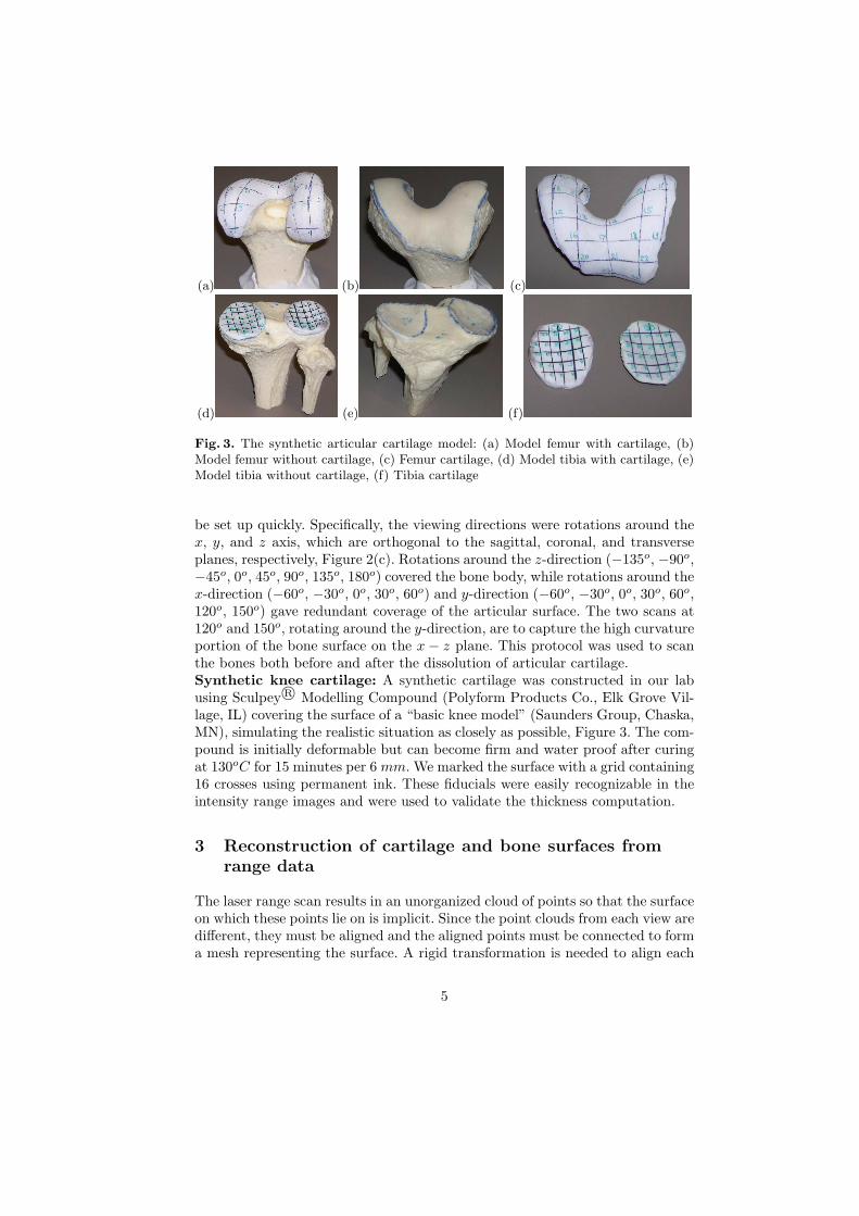
Fig. 3. The synthetic articular cartilage model: (a) Model femur with cartilage, (b)Model femur without cartilage, (c) Femur cartilage, (d) Model tibia with cartilage, (e)Model tibia without cartilage, (f) Tibia cartilage

be set up quickly. Specifically, the viewing directions were rotations around thex, y, and z axis, which are orthogonal to the sagittal, coronal, and transverseplanes, respectively, Figure 2(c). Rotations around the z-direction (−135o, −90o,−45o, 0o, 45o, 90o, 135o, 180o) covered the bone body, while rotations around thex-direction (−60o, −30o, 0o, 30o, 60o) and y-direction (−60o, −30o, 0o, 30o, 60o,120o, 150o) gave redundant coverage of the articular surface. The two scans at120o and 150o, rotating around the y-direction, are to capture the high curvatureportion of the bone surface on the x − z plane. This protocol was used to scanthe bones both before and after the dissolution of articular cartilage.Synthetic knee cartilage: A synthetic cartilage was constructed in our labusing Sculpey R© Modelling Compound (Polyform Products Co., Elk Grove Vil-lage, IL) covering the surface of a “basic knee model” (Saunders Group, Chaska,MN), simulating the realistic situation as closely as possible, Figure 3. The com-pound is initially deformable but can become firm and water proof after curingat 130oC for 15 minutes per 6 mm. We marked the surface with a grid containing16 crosses using permanent ink. These fiducials were easily recognizable in theintensity range images and were used to validate the thickness computation.

3 Reconstruction of cartilage and bone surfaces fromrange data

The laser range scan results in an unorganized cloud of points so that the surfaceon which these points lie on is implicit. Since the point clouds from each view aredifferent, they must be aligned and the aligned points must be connected to forma mesh representing the surface. A rigid transformation is needed to align each

5

(a) (b) (c) (d)

(e) (f) (g)

Fig. 4. The range images of a femur from 4 different viewing directions, shown indifferent colors (a, b, c, d). These point clouds are aligned using the ICP algorithm tobring all the images to one common coordinate system, (e). Next the range images aremerged to create a single triangular mesh, which often contains holes, junctions, anddisconnected parts, (f). These topological abnormalities are then removed to create asimple manifold surface of the bone, (g)

pair of range images. We use the Polyworks R© IMAlign [9] software to performthe alignment. The software requires a user to select a minimum of three pairsof corresponding points between the two scans to determine a rough estimateof the alignment. It then fine-tunes the alignment using a proprietary variant ofthe Iterative Closest Point (ICP) algorithm [10], which iteratively minimizes themean distance between the two scans at the overlapping regions. To ensure theICP algorithm’s reliability, we divided each image set into groups of adjacentviews and align images in each group separately. The groups are then alignedfollowing the same procedure as aligning the original scanned images. Althoughthis procedure theoretically brings all the range images into one common co-ordinate system, accumulative error due to the incremental alignment can besignificant because the number of images in each set is large. Thus, as a finalstep the ICP algorithm is applied on all the range images simultaneously to getthe optimal global alignment.

Next we use Polyworks R© IMMerge to merge the aligned range images intoone single triangular mesh representing the surface, Figure 4. The IMMerge soft-ware determines and discard the outlier points in the range images and createsa triangular mesh that minimizes the mean distance to the remaining points. Tosave processing time, we roughly outline the points close to our area of interest,the articular cartilage, and set the program to only merge those points.

Holes, cracks, and imperfections in the topology are common problems insurface construction from range images, particularly for rough surfaces like bonescovered with soft tissues, Figure 4(f). Many methods have been proposed to

6

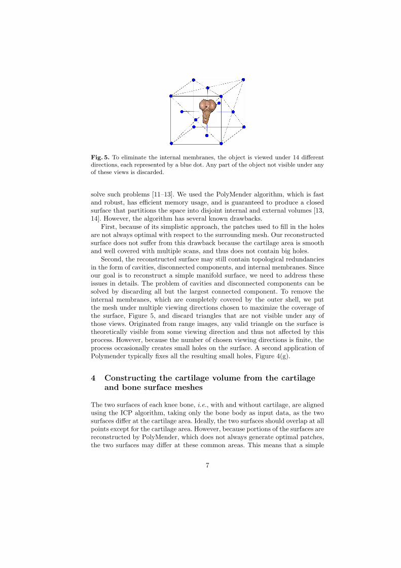
Fig. 5. To eliminate the internal membranes, the object is viewed under 14 differentdirections, each represented by a blue dot. Any part of the object not visible under anyof these views is discarded.

solve such problems [11–13]. We used the PolyMender algorithm, which is fastand robust, has efficient memory usage, and is guaranteed to produce a closedsurface that partitions the space into disjoint internal and external volumes [13,14]. However, the algorithm has several known drawbacks.

First, because of its simplistic approach, the patches used to fill in the holesare not always optimal with respect to the surrounding mesh. Our reconstructedsurface does not suffer from this drawback because the cartilage area is smoothand well covered with multiple scans, and thus does not contain big holes.

Second, the reconstructed surface may still contain topological redundanciesin the form of cavities, disconnected components, and internal membranes. Sinceour goal is to reconstruct a simple manifold surface, we need to address theseissues in details. The problem of cavities and disconnected components can besolved by discarding all but the largest connected component. To remove theinternal membranes, which are completely covered by the outer shell, we putthe mesh under multiple viewing directions chosen to maximize the coverage ofthe surface, Figure 5, and discard triangles that are not visible under any ofthose views. Originated from range images, any valid triangle on the surface istheoretically visible from some viewing direction and thus not affected by thisprocess. However, because the number of chosen viewing directions is finite, theprocess occasionally creates small holes on the surface. A second application ofPolymender typically fixes all the resulting small holes, Figure 4(g).

4 Constructing the cartilage volume from the cartilageand bone surface meshes

The two surfaces of each knee bone, i.e., with and without cartilage, are alignedusing the ICP algorithm, taking only the bone body as input data, as the twosurfaces differ at the cartilage area. Ideally, the two surfaces should overlap at allpoints except for the cartilage area. However, because portions of the surfaces arereconstructed by PolyMender, which does not always generate optimal patches,the two surfaces may differ at these common areas. This means that a simple

7

(a) (b)

(c) (d)

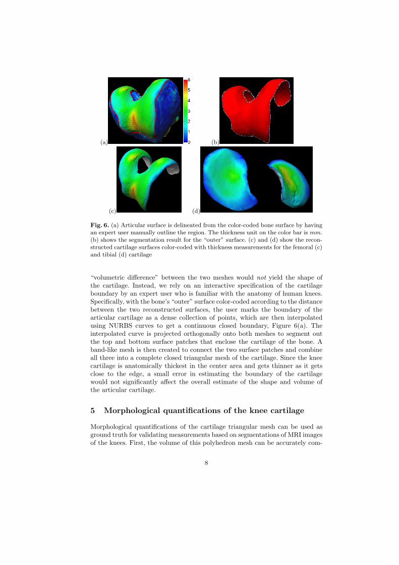
Fig. 6. (a) Articular surface is delineated from the color-coded bone surface by havingan expert user manually outline the region. The thickness unit on the color bar is mm.(b) shows the segmentation result for the “outer” surface. (c) and (d) show the recon-structed cartilage surfaces color-coded with thickness measurements for the femoral (c)and tibial (d) cartilage

“volumetric difference” between the two meshes would not yield the shape ofthe cartilage. Instead, we rely on an interactive specification of the cartilageboundary by an expert user who is familiar with the anatomy of human knees.Specifically, with the bone’s “outer” surface color-coded according to the distancebetween the two reconstructed surfaces, the user marks the boundary of thearticular cartilage as a dense collection of points, which are then interpolatedusing NURBS curves to get a continuous closed boundary, Figure 6(a). Theinterpolated curve is projected orthogonally onto both meshes to segment outthe top and bottom surface patches that enclose the cartilage of the bone. Aband-like mesh is then created to connect the two surface patches and combineall three into a complete closed triangular mesh of the cartilage. Since the kneecartilage is anatomically thickest in the center area and gets thinner as it getsclose to the edge, a small error in estimating the boundary of the cartilagewould not significantly affect the overall estimate of the shape and volume ofthe articular cartilage.

5 Morphological quantifications of the knee cartilage

Morphological quantifications of the cartilage triangular mesh can be used asground truth for validating measurements based on segmentations of MRI imagesof the knees. First, the volume of this polyhedron mesh can be accurately com-

8

puted [15]. Let the mesh have vertices P = {v1, v2, · · · , vn}, where vi = (xi, yi, zi)and triangular faces F = {f1, f2, · · · , fm}, where fi = (vi

1, vi2, v

i3) and assume

all the triangular faces are consistently oriented, the volume of the polyhedronmesh is computed as:

V =16

∑

fi∈F

∣∣∣∣∣∣

xi1 xi

2 xi3

yi1 yi

2 yi3

zi1 zi

2 zi3

∣∣∣∣∣∣where

vi1 = (xi

1, yi1, z

i1)

vi2 = (xi

2, yi2, z

i2)

vi3 = (xi

3, yi3, z

i3)

Second, the thickness of the cartilage is the distance between the two recon-structed (top and bottom) surface patches of the cartilage. This distance canbe defined (i) by using one surface as the reference surface and computing thedistance of the closest point or (ii) as the distance along the normal at eachpoint of the reference surface or (iii) by using the distance in the distance trans-form of the reference surface [6, 16, 18]. In this paper we adopt the first approachand use the algorithm in [17]. The triangles of the reference surface are dividedspatially into cubical cells to limit the search space in computing the distancebetween a point and the reference surface. The search is limited to only trianglesthat belong to the cells in a small neighborhood of the point. This algorithm hasbeen proven in practice to be faster than the brute-force method and allows forcomputing distances between two very large triangular meshes.

6 Results and Discussion

We treated the synthetic knee and cartilage models as if they were from a real ca-daver. The models were scanned, the scans were aligned and merged, a cartilagetriangular mesh was constructed, and its volume and thickness were computed.To validate our volume assessment, we measured the volumes of the syntheticcartilage using water displacement method and compare against the computedmeasurements, Table 1. The average discrepancy between the two measurementsis 5.2%. It is not clear to us which method is superior but the volume measure-ments from the laser scanning method are well within the variability of the waterdisplacement method.

Table 2 compares the volume measurements of the cadaver knees’ articularcartilage using the laser scanning method and using manual segmentation ofMR images. In the manual segmentation method, volume was computed by

Table 1. Comparison of volume measurements of articular cartilage using 3D laserscanner (LS) and by water displacement (WD). The WD values are the measurementsof three trials

Cartilage type LS Volume (ml) WD Volume (ml) Error (%)

Femoral cartilage 11.8 12.3±0.9 4.0Tibial cartilage 5.0 4.7±0.2 6.4

9

Table 2. Comparison of volume measurements of femoral (F) and tibial (T) cartilageusing 3D laser scanner and manual segmentation from 3T MR images

Cadaver 971 972 973 974 975F T F T F T F T F T

Volume - Laser scanner(ml) 14.5 4.9 10.7 5.8 9.4 4.6 2.9 1.9 8.8 3.1

Volume - Manual Seg. (ml) 13.1 5.6 9.3 4.2 10.7 4.8 2.2 1.6 7.2 3.2

Err(%) 9.7 14.3 13.1 29.3 13.8 4.3 24.1 15.8 19.3 3.2

simply counting the segmented cartilage voxels, and thus may not be accurate.Nevertheless, the two measurements are of the same order, which signifies theapplicability of the laser scanning method on cadavers.

As for validating thickness assessment, we measured the thickness of thecartilage model at fiducial points using a caliper and compared against thicknessmeasurements from the laser scanning method, Table 3 and Figure 7. We notethat at most points the caliper thickness measurements are slightly larger thanthose computed from the laser range scans. This is expected because measuringthickness using a caliper requires manually finding the points on the bottomsurface of the synthetic cartilage that are closest to the fiducial points. Thisprocess is generally difficult, especially when the surface is curvy, and any errorsincurred will only increase the caliper measurement values. Nevertheless, theaverage discrepancies between the two measurements for the femoral and tibialcartilage were 4.5% and 3.6 %, respectively. Given the accuracy and reliabilityof the laser scanner (50 µm) is superior to that of the MR imaging and assumingsimilar errors in segmentation, computed thickness from laser range scans areexpected to provide ground truth data for MR thickness measurements.

In a recent approach [19] a 3D laser scanner is similarly used to scan thefemur of three porcine knees, both with the cartilage intact and after it hadbeen dissolved. The result data were then used to validate the B-Spline Snakemethod used to segment knee cartilage from MR images. This approach and oursare similar in utilizing the 3D laser scanner but differ in the following aspects.First, our method determines a complete 3D mesh of the cartilage instead ofjust the thickness map. Second, in our approach it is not required to attachthe specimen to a frame; this allows for more freedom in choosing the scanningangles and reduces one source of error caused by the physical attachment betweenthe bone and the frame. In addition, we provide validation of our method on asynthetic cartilage model.

We have presented a method to accurately assess articular cartilage mor-phology using the 3D laser scanning technology. To use these measurementsas ground truth for segmentations from MR images, we note that care needsto be taken to preserve the morphological properties of the cartilage betweenthe time of MR scans and the time of laser scans and during laser scans, e.g.,regularly bathing the bones with physiological saline solution when they are ex-posed to the air to prevent the cartilage from drying out. We plan to validate

10

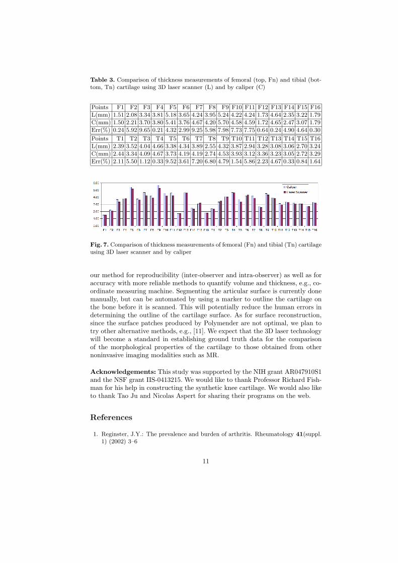
Table 3. Comparison of thickness measurements of femoral (top, Fn) and tibial (bot-tom, Tn) cartilage using 3D laser scanner (L) and by caliper (C)

Points F1 F2 F3 F4 F5 F6 F7 F8 F9 F10 F11 F12 F13 F14 F15 F16

L(mm) 1.51 2.08 3.34 3.81 5.18 3.65 4.24 3.95 5.24 4.22 4.24 1.73 4.64 2.35 3.22 1.79

C(mm) 1.50 2.21 3.70 3.80 5.41 3.76 4.67 4.20 5.70 4.58 4.59 1.72 4.65 2.47 3.07 1.79

Err(%) 0.24 5.92 9.65 0.21 4.32 2.99 9.25 5.98 7.98 7.73 7.75 0.64 0.24 4.90 4.64 0.30

Points T1 T2 T3 T4 T5 T6 T7 T8 T9 T10 T11 T12 T13 T14 T15 T16

L(mm) 2.39 3.52 4.04 4.66 3.38 4.34 3.89 2.55 4.32 3.87 2.94 3.28 3.08 3.06 2.70 3.24

C(mm) 2.44 3.34 4.09 4.67 3.73 4.19 4.19 2.74 4.53 3.93 3.12 3.36 3.23 3.05 2.72 3.29

Err(%) 2.11 5.50 1.12 0.33 9.52 3.61 7.20 6.80 4.79 1.54 5.86 2.23 4.67 0.33 0.84 1.64

Fig. 7. Comparison of thickness measurements of femoral (Fn) and tibial (Tn) cartilageusing 3D laser scanner and by caliper

our method for reproducibility (inter-observer and intra-observer) as well as foraccuracy with more reliable methods to quantify volume and thickness, e.g., co-ordinate measuring machine. Segmenting the articular surface is currently donemanually, but can be automated by using a marker to outline the cartilage onthe bone before it is scanned. This will potentially reduce the human errors indetermining the outline of the cartilage surface. As for surface reconstruction,since the surface patches produced by Polymender are not optimal, we plan totry other alternative methods, e.g., [11]. We expect that the 3D laser technologywill become a standard in establishing ground truth data for the comparisonof the morphological properties of the cartilage to those obtained from othernoninvasive imaging modalities such as MR.

Acknowledgements: This study was supported by the NIH grant AR047910S1and the NSF grant IIS-0413215. We would like to thank Professor Richard Fish-man for his help in constructing the synthetic knee cartilage. We would also liketo thank Tao Ju and Nicolas Aspert for sharing their programs on the web.

References

1. Reginster, J.Y.: The prevalence and burden of arthritis. Rheumatology 41(suppl.1) (2002) 3–6

11

2. Eckstein, F., Glaser, C.: Measuring cartilage morphology with quantitative mag-netic resonance imaging. Seminars in Musculoskeletal Radiology 8(4) (2004) 329–53

3. Ateshian, G.A., Soslowsky, L.J., , Mow, V.C.: Quantitation of articular surfacetopography and cartilage thickness in knee joints using stereophotogrammetry.Journal of Biomechanics 24(8) (1991) 761–776

4. Berquist, T.H.: Imaging of articular pathology: MRI, CT, arthrography. ClinicalAnatomy 10(1) (1997) 1–13

5. Gandy, S.J., Dieppe, P.A., Keen, M.C., Maciewicz, R.A., Watt, I., Waterton, J.C.:No loss of cartilage volume over three years in patients with knee osteoarthritisas assessed by magnetic resonance imaging. Osteoarthritis and Cartilage 10(12)(2002) 929–937

6. Cohen, Z.A., McCarthy, D.M., Kwak, S.D., Legrand, P., F., F., Ciaccio, E.J.,Ateshian, G.A.: Knee cartilage topography, thickness, and contact areas frommri: in-vitro calibration and in-vivo measurements. Osteoarthritis and Cartilage7(1) (1999) 95–109

7. Son, S., Park, H., Lee, K.H.: Automated laser scanning system for reverse engi-neering and inspection. International Journal of Machine Tools and Manufacture42(8) (2002) 889–897

8. Milroy, M.J., Weir, D.J., Bradley, C., Vickers, G.W.: Reverse engineering em-ploying a 3d laser scanner: A case study. The International Journal of AdvancedManufacturing Technology 12(2) (1996) 111 – 121

9. Innovmetric Software Incorporation: Product manual.http://www.shapegrabber.com (2006)

10. Besl, P.J., McKay, N.D.: A method for registration of 3D shapes. IEEE Trans. Pat-tern Analysis and Machine Intelligence 14(2) (1992) 239–256

11. Davis, J., Marschner, S., Garr, M., Levoy, M.: Filling holes in complex surfacesusing volumetric diffusion. In: Proceedings of First International Symposium on3D Data Processing, Visualization, and Transmission. (2002)

12. Nooruddin, F., Turk, G.: Simplification and repair of polygonal models using vol-umetric techniques. IEEE Transactions on Visualization and Computer Graphics9(2) (2003) 191–205

13. Ju, T.: Robust repair of polygonal models. ACM Trans. Graph. 23(3) (2004)888–895

14. Ju, T.: Polymender. http://www.cs.rice.edu/ jutao/code/polymender.htm (2006)15. Gelder, A.V.: Efficient Computation of Polygon Area and Polyhedron Volume. In:

Graphics Gems V. AP Professional (1995)16. Hardy, P.A., Nammalwar, P., Kuo, S.: Measuring the thickness of articular cartilage

from mr images. Journal of Magnetic Resonance Imaging 13(1) (2001) 120–617. Aspert, N., Santa-Cruz, D., Ebrahimi, T.: Mesh: Measuring errors between surfaces

using the hausdorff distance. In: Proc. of the IEEE International Conference inMultimedia and Expo (ICME). (2002) 705–708

18. Stammberger, T., Eckstein, F., Englmeier, K.H., Reiser, M.: Determination of3d cartilage thickness data from MR imaging: computational method and repro-ducibility in the living. Magnetic Resonance in Medicine 41(3) (1999) 529–36

19. Koo, S., Gold, G.E., Andriacchi, T.P.: Considerations in measuring cartilage thick-ness using MRI: factors influencing reproducibility and accuracy. Osteoarthritisand Cartilage 13(9) (2005) 782–9

12