achieveable total-to-static efficiencies of low pressure ... · achieveable total-to-static...

ACHIEVEABLE TOTAL-TO-STATIC EFFICIENCIES OF LOW PRESSURE AXIAL FANS

Konrad BAMBERGER, Thomas CAROLUS,

Institute for Fluid- and Thermodynamics, University of Siegen, Paul-Bonatz-Str. 9-11, 57068 Siegen, Germany

SUMMARY

The achievable total-to-static efficiency of low pressure axial fans is estimated as a function of design point. In a first step, all hydraulic losses are neglected such that the target of maximum total-to-static efficiency equals the minimization of exit losses. Minimal exit losses are found by optimizing the hub-to-tip ratio and the load distribution. A more realistic estimation is obtained by predicting the fan performance with CFD-trained artificial neural networks (ANNs) which are coupled with an evolutionary optimization algorithm. The ANNs were obtained from earlier studies by the authors of this work. Finally, the ANN-based optimization is repeated with con-strained input space to estimate the impact of practical restrictions on the achievable efficiency.

NOMENCLATURE

Latin symbols

A area

D diameter

P power

V& flow rate

a, b swirl distribution parameters

c flow velocity

n fan speed

p pressure

r radius

u circumferential fan speed

Greek Symbols

α weighting factor for penalty term

δ specific fan diameter

φ flow coefficient

φc velocity coefficient

η efficiency

ν hub-to-tip ratio

ρ air density

σ specific fan speed

ψ pressure coefficient

FAN 2015 2 Lyon (France), 15 – 17 April 2015

Indices

1 upstream of the fan

2 downstream of the fan

c flow velocity

dyn dynamic

ini initialization

m meridional

opt optimal

t total

ts total-to-static

tt total-to-total

θ circumferential

Abbreviations

ANN Artificial Neural Network

CFD Computational Fluid Dynamics

MLP Multi-Layer Perceptron

RANS Reynolds-averaged Navier-Stokes

INTRODUCTION

A typical design target of low-pressure axial fans is meeting a design point (pressure rise ∆p at a specific flow rate V& ) with the lowest possible shaft power Pshaft. Often, the kinetic energy down-stream of the fan cannot be recovered and hence must be considered as exit loss. In that case, the target of minimal shaft power equals the maximization of total-to-static efficiency defined as

tsts

shaft

V p.

P

∆η ≡&

(1)

"Total-to-static" means that the pressure difference is calculated assuming total pressure upstream of the fan (index "1") but static pressure downstream of the fan (index "2"):

2 1ts tp p p∆ = − (2)

Instead of the term "total-to-static pressure/efficiency", the short term "static pressure/efficiency" is also in common usage. Even if the kinetic energy in the outflow is partly recovered by guide vanes and/or diffusers, it is useful to design impellers with high total-to-static efficiency in order to reduce the load of the auxiliary components. This generally helps to design them more compactly and to enhance their efficiency.

Minimum efficiency requirements for fans on the European market are defined by the European Commission Regulation 327/2011 [1]. In this document, the minimum efficiency requirements are linked to the power of the electrical motors driving the fan. Such an approach takes into account that the efficiency of electric motors typically increases with motor power. On top of that, defining minimum efficiencies based on the driving power indirectly accounts for Reynolds effects as pow-erful motors coincide with large or swiftly rotating fans, i.e. fans with high Reynolds numbers. Typically, higher Reynolds numbers lead to reduced hydraulic losses which justifies stricter effi-ciency requirements.

However, the achievable total-to-static efficiency is also strongly affected by the design point. For instance, fans designed for high flow rates always feature increased exit losses. The design point is not considered in the European regulation. This study aims at the estimate of achievable total-to-static efficiencies as a function of the design point of axial fans without guide vanes and diffusers.

Throughout this work, the design point is expressed in a non-dimensional way, i.e. V& and ∆p are normalized with the outer fan diameter D, the rotational speed n and the air density ρ yielding the flow coefficient φ and pressure coefficient ψ, respectively:


23

4

V

D nφ π≡

&

(3)

22 2

2

p

D n

∆ψ π ρ≡ (4)

Another way to express the non-dimensional design point is to normalize n and D yielding the spe-cific fan speed σ and the specific fan diameter δ, respectively:

( )3 4

1 42 1 22/

/ /tt

n

pV

σ∆πρ

− −

≡

&

(5)

1 41 4

1 2

2

8//

/tt

D

pV

δ∆

π ρ

−≡

&

(6)

Note that σ and δ are always computed with the total-to-total pressure rise ∆ptt = pt2 - pt1. Two ve-locity components at the blade cascade exit plane are important: The meridional component cm and the circumferential component cθ. Velocities are normalized with the tip speed utip = πnD in order to obtain the meridional and circumferential velocity coefficients φc ≡ c/utip. The dimensionless exit loss is computed as the flow-rate averaged local dynamic pressure in the exit plane:

( )

( )2

2 22

2 22 2

2 22 2

2 2

112

2

m

mA

dyn , c cA

c c dVV dV

VD nθ

θρ

ψ φ φπ ρ

+∫ ≡ = + ∫

&&

&&

(7)

The jet/wake structure of the flow in the exit plane is assumed to be levelled out and hence constant in circumferential direction. Thus, only the spanwise distribution of φc between hub and tip is rele-vant and dV& is equivalent with 2 2mc r drπ⋅ ⋅ . Replacing V& with the flow coefficient φ (Eq. 3) and introducing the dimensionless radius r* = r/rtip = 2r/D, eventually yields an equation for the exit losses which is based on non-dimensional quantities only:

( )2 2 2

12 2

2

2m m

* *dyn , c c c r dr

θν

ψ φ φ φφ

= +∫ (8)

In this equation, the lower bound of integration is the hub-to-tip ratioν = rhub / rtip. Given the exit loss, the total-to-static efficiency can be computed as

2tt dyn ,

ts tt

tt

.ψ ψ

η ηψ−

= (9)

The objective of this work is to estimate the achievable total-to-static efficiency for numerous de-sign points in three different ways:

a) Assuming a number of simplifications (most importantly neglecting hydraulic losses, i.e. ηtt = 1) the only remaining loss is the exit loss according to Eq. 8. This approach is used to find the theoretical value of minimum exit loss and eventually a first estimate of maximum total-to-static efficiency.


b) In order to obtain more realistic results, the hydraulic loss is then taken into account by predict-ing the total-to-static efficiency with artificial neural networks (ANN) which were trained on the basis of CFD-simulations in an earlier study [2]. The ANNs are coupled with an evolutionary optimization algorithm with the target function of maximum total-to-static efficiency for given design points. By this approach, exit and hydraulic losses are minimized in the sense that their sum becomes minimal.

c) Finally, the ANN approach b) is repeated but with technically relevant geometrical constraints which are (i) fixed sweep angles, (ii) limited axial depth of the rotor and (iii) avoidance of un-dercuts.

METHODOLOGY

The investigations shall be conducted with typical design point targets of low pressure axial fans. In 1953, Cordier [3] found that the optimal design points of all fans and pumps of his time are located in a narrow band in the σ-δ diagram, later known as the Cordier diagram or Cordier band. In 2012, Pelz [4] analyzed the theoretical background of Cordier's findings and derived a formula for a curve in the σ-δ diagram which approaches the original Cordier band:

2

23 3

1 1 1

22 2opt

optopt opt

σψδφδ φδ

= + +

) ) ) (10)

The quantities φ)and ψ) determine the asymptotes of the curve. In the present study, the values φ

)=

0.25 and ψ) = 1 will be used which is an adequate choice according to Pelz. Commonly, axial fans

are designed in the range between 0.5 ≤ σopt ≤ 2. Fans with smaller specific speed are typically of centrifugal type while larger specific speeds are the realm of propellers. In this study, we focus on the interval 0.5 ≤ σopt ≤ 2 and compute the corresponding specific diameter δopt according to Eq. 10. δ is varied between 0.8.δopt ≤ δ ≤ 1.2.δopt to obtain a band in the σ-δ diagram. Figure 1 shows the σ-δ diagram and indicates the section of the band considered in this work. Within this section, the achievable total-to-static efficiency is computed in three different ways which are described below.

a) Theoretical maximum total-to-static efficiency: The total-to-static efficiency is computed with Eq. 9, hence ψtt, ηtt and ψdyn2 must be known. Since we consider hydraulically perfect ("theoreti-

0.1 0.5 1 2 31

2

4

6

810

Considered sectionof Cordier band

Cordier curveaccording to Eq. 10

σ [-]

δ [-

]

Figure 1: Cordier curve with indication of the section considered for the present investigations


cal") fans we assume ηtt = 1. ψtt is a direct consequence of the targeted design point and hence given. Thus, the only unknown quantity is the exit loss, ψdyn,2. It can be computed with Eq. 8 which, however, requires ν,

2mcφ (r*), and 2cφφ (r*). The spanwise distribution of

2cφφ (swirl distribution) is

assumed to have a shape as suggested by Horlock [5]:

( )2

*c *

br a ,

rθφ = + (11)

The task is now to find the swirl distribution parameters a and b that yield minimum exit losses and hence maximum total-to-static efficiency. However, a and b cannot be selected freely due to the constraint that the design point must be fulfilled. Firstly, the

2cφφ (r*) distribution must be consistent

with the overall pressure coefficient of the targeted design point. The dimensional pressure rise is computed by Eq. 12:

( )2

1tt tt

A

p p r dVV

∆ ∆= ⋅∫ &&

(12)

The local pressure rise ∆ptt(r) can be calculated by the Euler equation of turbomachinery, i.e.

( ) ( )22ttp r rn c rθ∆ ρ π= ⋅ ⋅ . (13)

With the definitions of non-dimensional quantities as introduced above, the pressure coefficient be-comes

2

2 2

2 2 2 1

22 2

12

4

2

m

mA * * *

tt c c

rn c c dAV r r dr

D nθ

θ

ν

ρ πψ φ φ

π φρ

⋅ ⋅ ⋅∫ ≡ = ∫

&. (14)

The problem with Eq. 14 is that it contains the distribution of the meridional flow coefficient

2mcφ (r*) which is still unknown. However, 2mcφ (r*) and

2cφφ (r*) can be related to each other via the so-

called simple radial equilibrium in the exit flow. The corresponding differential equation, e.g. de-scribed by Dixon [6], is non-dimensionalized for the present purpose:

( ) ( )2 22 2

2

m

m

* *c cc c

c* * * *

d r d r d

dr r dr drθ θθ

φ φφ φφ= + (15)

The second constraint with respect to the design point is that the 2mcφ (r*) distribution must be consis-

tent with the targeted flow coefficient:

2

1

2m

* *c r dr

νφ φ= ∫ (16)

Altogether, the target can be summarized as follows: Find the swirl distribution parameters a and b as well as the hub-to-tip ratioν which minimize the exit losses according to Eq. 8 while exactly ful-filling the targeted design point according to Eq. 14 and 16. The solution of this non-linear minimi-zation problem is found by the Simplex method by Nelder and Mead [7]. Since this method is a lo-cal optimization algorithm, adequate initialization is required. A medium start value for the hub-to-tip ratio is selected (νini = 0.5). The well-known free-vortex design method is used for the initial swirl distribution, i.e. aini = 0 and hence

2

*c rφφ ⋅ = bini. The magnitude of bini is selected such that the

desired pressure coefficient is fulfilled. b) Optimization of total-to-static efficiency based on artificial neural networks: In this ap-proach, the total-to-static efficiency for each design point is optimized by an evolutionary optimiza-


tion algorithm. The evaluation of the target function is conducted by artificial neural networks, or more specifically by multi layer perceptrons (MLP). As mentioned in the introduction, the MLPs used here are based on a previous study by the authors in 2014. For that reason, the following de-scription of the training strategy is kept very short. All details can be found in reference [2]. 26 geometrical parameters were defined and varied by a space-filling Design of Experiments (DoE). The tip clearance did not belong to those parameters but was kept constant and amounted to S/D = 0.1%. The characteristic performance curve of each fan design was obtained by means of Reynolds-averaged Navier-Stokes (RANS) simulations with the shear stress transport (SST) turbulence model. For the simulation, D = 0.3 m and n = 3000 min-1 was selected yielding Reynolds numbers around 200,000. The computational grid consisted of approximately 500,000 hexahedral nodes and only one blade channel was simulated with periodic boundary conditions at the sides. The grid in-dependence was proven by simulating aerodynamically optimized fans with considerably finer grids containing up to 2,000,000 nodes. It was found that the discretization error with respect to η and ψ is less than 1%. The final CFD database contains around 13,000 fan curves and was used to train the MLPs. The MLPs consist of the input layer, two hidden layers with sigmoid neurons and one output layer with linear neurons. Optimization of the hidden layer weights was done with the MATLAB Neural Network Toolbox which uses the Levenberg-Marquandt algorithm [8]. Network structure optimization (the number of neurons in each hidden layer) was done by an in-house algorithm based on the principle ideas of the steepest descent method. For each design point, the target function is maximization of ηts as predicted by the MLPs. Viola-tion of the desired pressure coefficient is considered by a penalty term:

*

ts ,MLP predicted tt tt ,MLP predictedη η α ψ ψ− −= − − (17)

The empiric weighting factor α of the penalty term is set to 5. Since the function evaluation by means of MLPs is extremely quick, it is affordable to use a huge number of individuals per genera-tion and a huge number of generations (10,000 each) within the evolutionary algorithm to ensure that the global optimum is found. c) Optimization of total-to-static efficiency with geometrical constraints: The optimization strategy b) is extended by the consideration of three typical geometrical constraints.

1. For acoustic reasons, the blades of axial fans are often swept. However, aerodynamically op-timal designs often have no or only moderate sweep angles as shown in [9]. To examine the aerodynamic impact of sweep, strong sweep angles are imposed and only the other geomet-rical parameters are varied in the optimization process. The sweep angles used for this study amount to -50° at the hub, +30° at midspan, and +50° at the tip. The full description how sweep angles are geometrically implemented can be found in [2].

2. In many applications, the available space is limited which leads to fans which are shorter in axial depth than suggested by an unconstrained optimization. In the example investigated here, the allowable axial depth is restricted by lax < 0.2D which is implemented by a penalty term for individuals with longer axial depth.

3. If the fan is manufactured by die-casting, it might be necessary to avoid undercuts such that the tools can be separated in a purely axial direction. This is implemented by a penalty term for individuals with overlapping blades (in front view).


RESULTS

Theoretically achievable total-to-static efficiency

The left plot in Figure 2 shows the achievable total-to-static efficiency ηts,th according to approach a). As expected, the highest theoretical efficiencies are found at large specific fan diameters which reduce the averaged throughflow velocity and thus mitigate exit losses. Another tendency which can be observed is that the theoretical efficiency also increases with specific fan speed. This can be ex-plained by Euler's equation (Eq. 13) which states that the circumferential flow velocity may be smaller if the circumferential blade velocity is high. The maximum value of ηts is found at the top left corner of the selected portion of Cordier's band and amounts to approximately 83 %.

On the right-hand side of Figure 2, the optimal load distribution is analyzed. For that, the normal-ized load distribution coefficient a* is introduced. It is linked to the load distribution coefficients introduced above via Eq. 18:

2* tt

tt

ba

ψψ−= (18)

The advantage of using a* is that its magnitude is intuitively interpretable. It becomes zero for isoenergetic load distribution ("free-vortex", rcθ2 = const.) and unity for cθ2 = const. a* > 1 refers to increasing circumferential velocity from hub to tip. The pursuit of optimal load distribution requires balancing of two competing effects. On the one hand, a* should be high since shifting load towards the outer blade region reduces the required circumferential flow velocity according to the Euler equation. On the other hand, only a* = 0 leads to a completely even throughflow with

2mcφ (r*) =

const., see Eq. 15. If a* exceeds the optimum, the additional exit losses due to the uneven profile of

2mcφ overcompensate the advantages regarding losses associated with 2cθφ . Reducing losses associ-

ated with 2cθφ is most important if the specific fan speed and the specific fan diameter are low be-

cause much swirl is required for such design points. This is reflected by large values of a* in the bottom-left corner of the Cordier band, see Figure 2. Towards large specific fan speeds and large specific fan diameters, a* approaches zero meaning that almost isoenergetic load distributions be-come increasingly advantageous. In reality, the free-vortex designs are even more favorable because an even velocity profile of

2mcφ (r*) also helps to keep hydraulic losses low. This was shown in a re-

cent study by Bamberger and Carolus [10].

Figure 3 presents a closer look at the exit losses and distinguishes between losses associated with

2mcφ or with 2cθφ . The contour plots show the loss in efficiency due to the two loss mechanisms:

0.5 1 21

2

3

σ [-]

δ [-

]

ηts,th [-]

0

0.2

0.4

0.6

0.8

0.5 1 21

2

3

σ [-]

a* [-]

0

0.2

0.4

0.6

0.8

1.0

1.2

Figure 2: Theoretically achievable total-to-static efficiency (left) and optimal load distribution coefficient a* (right)


2 2

2 2 and m

m

dyn ,c dyn ,c

ts ,c ts ,c

tt tt

θθ

ψ ψ∆η ∆η

ψ ψ= = (19)

Figure 3 emphasizes basic observations already described, e.g. high losses due to low specific fan speeds and/or diameters. In addition, Figure 3 provides quantitative information about the losses. On the average,

2mts ,c∆η is more relevant and reaches values up to 85%. Nevertheless, design points

exist where 2ts ,cθ∆η is much more significant than

2mts ,c∆η .

Realistically achievable total-to-static efficiency

Figure 4 shows the achievable total-to-static efficiency employing approach b). As mentioned be-fore, the evaluation of the target function was conducted by artificial neural networks of the MLP type. The optimized designs were simulated by CFD to verify the correctness of the MLP predic-tion. The subsequent plots are based on the CFD simulations of the optimized fans and conse-quently the associated efficiency is termed ηts,CFD. The CFD model used for these simulations is the same as used for training the MLPs. The maximal values of ηts,CFD are around 68 % and occur at the upper limit of the specific fan diameters and at medium specific fan speeds. This is consistent with an earlier study by the authors of this work [2]. The right-hand side of Figure 4 shows the difference between the theoretically achievable efficiency (Figure 2) and the CFD results. The minimal differ-ence is around eight percentage points and occurs at low specific fan diameters and medium spe-cific fan speeds. The maximum difference (around 18 percentage points) is found at design points where the theoretical efficiency is very high, i.e. at large specific fan diameters. Figure 5 allocates

0.5 1 21

2

3

σ [-]

δ [-

]

∆ηts,φc

m2

[-]

0

0.2

0.4

0.6

0.8

0.5 1 21

2

3

σ [-]

∆ηts,φc

θ2

[-]

0

0.1

0.2

0.3

Figure 3: Exit losses associated with throughflow velocity (left) and circumferential velocity (right)

0.5 1 21

2

3

σ [-]

δ [-

]

ηts,CFD [-]

0

0.2

0.4

0.60.68

0.5 1 21

2

3

σ [-]

ηts,th - ηts,CFD [-]

0

0.1

0.2

0.3

Figure 4: Achievable total-to-static efficiency according to MLP-optimization (left) and difference to the theoreti-

cally achievable total-to-static efficiency (right)


the difference in ηts to three effects. The left-hand side shows the efficiency drop due to hydraulic losses. Hydraulic losses arise from friction and increase with specific fan diameter as the reduction of momentum in the throughflow velocity favors the generation of secondary flows. In order to compensate the pressure drop due to friction, additional blade load is required resulting in addi-tional exit losses associated with

2cθφ , see right-hand side of Figure 5. Another reason for increased

exit losses associated with 2cθφ is the fact that the practical optimization shifts less load towards the

outer blade region as compared with the theoretical optimization. Reasons why the practical optimi-zation yields results with a more free-vortex-like load distribution are given in [10]. The plot in the middle of Figure 5 deals with additional exit losses associated with

2mcφ . It can be observed that at

almost all design points the theoretical and the practical optimization lead to almost identical losses. Hence, the potential for reducing the exit loss by using small hub-to-tip ratios is almost fully ex-ploited by the practical optimization. If no optimization algorithms are used, the hub size must be estimated conservatively, e.g. using the validity criteria by de Haller, Strscheletzky, and Lieblein (summarized by Carolus in [11]). The criterion by Strscheletzky is also the basis for a recommenda-tion about the optimal hub-to-tip ratio by Marcinowski [12]. The basic idea was to use a hub size which is only just as large as the dead wake core. Although the investigations by Marcinowski are rather old (from 1956) they are still of high relevance today. For instance, the famous textbook about fan design by Eck [13] still presents the Cordier diagram with curves of constant hub-to-tip ratio which are based on the work by Marcinowski. Figure 6 compares the hub-to-tip ratios obtained with the three different strategies. In the left part of the considered part of the Cordier band, there is a clear trend of decreasing hub size from the recommendation by Marcinowski over the practical optimization to the theoretical optimization. The magnitude of the exit losses associated with

2mcφ

decreases accordingly, but the difference between the practical and the theoretical optimization is marginal as it was revealed by Figure 5. However, this trend does not hold true for very small spe-cific fan diameters where the practical optimization always yields ν = 0.3 which is not the aerody-namic optimum but just the lower limit of the parameter space with which the MLPs were trained. As a consequence, the optimal hub-to-tip ratio according to the practical optimization exceeds the recommendation by Marcinowski in that area and will most likely be associated with higher exit losses. The comparison with the theoretical optimization reveals that the magnitude of the addi-tional exit losses can be as high as 15 percentage points.

Achievable total-to-static efficiency under geometrical constraints

Geometrical constraints reduce the achievable efficiency as some parameters are forced to differ from their aerodynamically optimal value. Figure 7 quantifies this effect by showing the difference

0.5 1 21

2

3 Frictionlosses

σ [-]

δ [-

]

0.5 1 21

2

3 Add. exitlosses (φc

m2

)

σ [-]0.5 1 21

2

3 Add. exitlosses (φc

θ2

)

σ [-]

∆ηts [-]

0

0.03

0.06

0.09

0.12

0.15

0.18

Figure 5: Difference between theoretically achievable and MLP-optimized total-to-static efficiency, subdivided into

hydraulic friction losses (left) and additional exit losses associated with 2mcφ (middle) or

2cθφ (right)


between an unconstrained optimization (see previous section) and optimizations with the three dif-ferent constraints described in the methodology section. Note that the contour plots in Figure 7 use the same color for all efficiency differences higher than five percentage points.

The left plot deals with the impact of strong sweep angles. Since the optimization algorithm adjusts all other geometrical parameters to the imposed sweep angles, the efficiency drop is not very high and hardly exceeds three percentage points. In medium regions of the Cordier band, the penalty is even close to zero which means that the sweep strategy may be determined by acoustic considera-tions only. Towards the bounds of the Cordier band the unconstrained optimization uses sweep an-gles to facilitate such extraordinary design points. Hence, in these regions fixing the sweep angles leads to a more significant drop in efficiency.

The effect of restricting the axial depth is addressed in the middle plot in Figure 7. At large specific fan diameters the stagger angles are very flat and lax < 0.2D is also fulfilled by the unconstrained optimization. At smaller specific fan diameters, the stagger angles become steeper and restricting lax can compromise the total-to-static efficiency by up to 14 percentage points. Regarding specific fan speed, the same trends can be observed, i.e. the penalty increases with decreasing fan speed. This can be explained by Euler's equation which states that in case of small circumferential blade veloci-ties more flow deflection is required to obtain the targeted pressure rise. As a consequence, design points with small specific fan speeds are usually realized with long chord lengths and hence with a high axial depth. The combination of small σ and small δ even makes it impossible to realize fans with lax < 0.2D which is indicated by the blank area in the Cordier band depicted in Figure 7.

Highly loaded blades are also problematic for the design of fans without undercuts. Hence, the effi-ciency drop due to avoidance of undercuts is most relevant in the region of small specific fan speeds. Regarding specific fan diameter, small values are preferable as this leads to steeper stagger angles and a weaker tendency for undercuts. It is remarkable that almost all fans obtained from un-constrained optimization have undercuts such that only in a very small area the efficiency drop be-tween unconstrained and constrained optimization approaches zero. Nevertheless, all design points investigated can also be realized without undercuts and the penalty due to avoidance of undercuts never exceeds five percentage points.

Figure 8 gives a visual impression of the fans designed with and without constraints. The design point selected for this example is σ = 1 and δ = 1.8. The left-hand side always shows the uncon-strained solution but in different views. On the right-hand side, the solutions for the three distinct constraints are shown.

0.5 1 21

2

3

Marcinowski

σ [-]

δ [-

]

0.5 1 21

2

3

Optimized

σ [-]0.5 1 21

2

3

Theoretical

σ [-]

νopt [-]

0

0.2

0.4

0.6

0.75

Figure 6: Optimal hub-to-tip ratio according to Marcinowski [12] (left),

MLP-optimization (middle) and theoretical optimization (right)


0.5 1 21

2

3

Fixed sweep

σ [-]

δ [-

]

0.5 1 21

2

3

lax < 0.2D

σ [-]0.5 1 21

2

3

No undercuts

σ [-]

∆ηts [-]

0

0.01

0.02

0.03

0.04

>0.05

Figure 7: Efficiency penalty due to geometrical constraints as predicted by the MLPs

No constraints

Constraint 1: Fixed sweep angle

No constraints

Constraint 2: lax ≤ 0.2D

No constraints

Constraint 3: No undercuts

Figure 8: Optimal fans for σ = 1 and δ = 1.8 without constraints (left) and with distinct constraints (right)


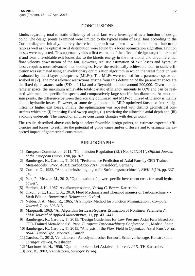
CONCLUSIONS

Limits regarding total-to-static efficiency of axial fans were investigated as a function of design point. The design points examined were limited to the typical realm of axial fans according to the Cordier diagram. Initially, a purely theoretical approach was taken in which the optimal hub-to-tip ratio as well as the optimal swirl distribution were found by a local optimization algorithm. Friction losses were neglected. This approach yields a first estimate of the effect of design target in terms of σ and δ on unavoidable exit losses due to the kinetic energy in the meridional and circumferential flow velocity downstream of the fan. However, realistic estimation of exit losses and hydraulic losses requires more advanced methodologies. Here, the realistically achievable total-to-static effi-ciency was estimated using an evolutionary optimization algorithm in which the target function was evaluated by multi-layer perceptrons (MLPs). The MLPs were trained for a parameter space de-scribed in [2]. The most relevant restrictions arising from this definition of the parameter space are the fixed tip clearance ratio (S/D = 0.1%) and a Reynolds number around 200,000. Given the pa-rameter space, the maximum achievable total-to-static efficiency amounts to 68% and can be real-ized with medium specific fan speeds and comparatively large specific fan diameters. At most de-sign points, the difference between theoretically optimized and MLP-optimized efficiency is mainly due to hydraulic losses. However, at some design points the MLP-optimized fans also feature sig-nificantly higher exit losses. Finally, the optimization was repeated with distinct geometrical con-straints which are (i) imposing fixed sweep angles, (ii) restricting the allowable axial depth and (iii) avoiding undercuts. The impact of all three constraints changes with design point.

The results described above can help to select favorable design points, to estimate expected effi-ciencies and losses, to estimate the potential of guide vanes and/or diffusers and to estimate the ex-pected impact of geometrical constraints.

BIBLIOGRAPHY

[1] European Commission, 2011, "Commission Regulation (EU) No. 327/2011", Official Journal of the European Union, L90, pp. 8-21.

[2] Bamberger, K., Carolus, T., 2014, "Performance Prediction of Axial Fans by CFD-Trained Meta-Models", Proc. ASME TurboExpo 2014, Düsseldorf, Germany.

[3] Cordier, O., 1953, "Ähnlichkeitsbedingungen für Strömungsmaschinen", BWK, 5(10), pp. 337-340.

[4] Pelz, P., Metzler, M., 2012, "Optimization of power-specific investment costs for small hydro-power".

[5] Horlock, J. H., 1967, Axialkompressoren, Verlag G. Braun, Karlsruhe. [6] Dixon, S. L., Hall, C. A., 2010, Fluid Mechanics and Thermodynamics of Turbomachinery -

Sixth Edition, Butterworth Heinemann, Oxford. [7] Nelder, J. A., Mead, R., 1965, "A Simplex Method for Function Minimization", Computer

Journal, 7, pp. 308-313. [8] Marquardt, 1963, "An Algorithm for Least-Squares Estimation of Nonlinear Parameters",

SIAM Journal of Applied Mathematics, 11, pp. 431-441. [9] Bamberger, K., Carolus, T., 2015, "Design Guidelines for Low Pressure Axial Fans Based on

CFD-Trained Meta-Models", Proc. European Turbomachinery Conference 11, Madrid, Spain. [10] Bamberger, K., Carolus, T., 2015, "Analysis of the Flow Field in Optimized Axial Fans", Proc.

ASME TurboExpo, Montreal, Canada. [11] Carolus, T., 2012, Ventilatoren - Aerodynamischer Entwurf, Schallvorhersage, Konstruktion,

Springer Vieweg, Wiesbaden. [12] Marcinowski, H., 1956, "Optimalprobleme bei Axialventilatoren", PhD, TH Karlsruhe. [13] Eck, B., 2003, Ventilatoren, Springer Verlag.

achieveable total-to-static efficiencies of low pressure ... · achieveable total-to-static...

Documents