iii

CONTENTS   

Acknowledgments................................................................................................................................................vii  

Executive Summary............................................................................................................................................... ix  SESSION 1: EMERGENCY PREPAREDNESS AND SURVEILLANCE  

Introduction to Session 1 Trena M. Ezzati‐Rice................................................................................................................................................. 1  

Real‐Time Data Dissemination in a Rapidly Changing Environment Allison D. Plyer, Denice Warren, and Joy Bonaguro ............................................................................................... 3  

Methods to Improve Public Health Responses to Disasters Paul Pulliam, Melissa Dolan, and Elizabeth Dean ................................................................................................... 9  

The Electronic Data Capture System Used to Monitor Vaccines during the U.S. Army’s Smallpox Vaccination Campaign Judith H. Mopsik, John D. Grabenstein, Johnny Blair, Stuart S. Olmsted, Nicole Lurie, Pamela Giambo, Pamela Johnson, Rebecca Zimmerman, and Gustavo Perez‐Bonany ...................................................................... 17  

Conducting Real‐Time Health Surveillance during Public Health Emergencies: The Behavioral Risk Factor Surveillance System Experience Michael W. Link, Ali H. Mokdad, and Lina Balluz ................................................................................................ 25  

Methodological Issues in Post‐disaster Mental Health Needs Assessment Research Ronald C. Kessler, Terence M. Keane, Ali Mokdad, Robert J. Ursano, and Alan M. Zaslavsky............................ 33  

Session 1 Summary Kathleen S. O’Connor and Michael P. Battaglia..................................................................................................... 45  SESSION 2: MEASUREMENT ERRORS AND HEALTH DISPARITIES  

Session 2 Introduction Timothy P. Johnson ................................................................................................................................................. 53  

Measurement Equivalence for Three Mental Health Status Measures John A. Fleischman .................................................................................................................................................. 55  

Reliability and Validity of a Colorectal Cancer Screening (CRCS) Questionnaire by Mode of Survey Administration Sally W. Vernon, Jasmin A. Tiro, Rachel W. Vojvodic, Sharon P. Coan, Pamela M. Diamond, and Anthony Greisinger ................................................................................................................................................. 63  

Reliability and Data Quality in the National Survey on Drug Use and Health Joel Kennet, Joe Gfroerer, Peggy Barker, Lanny Piper, Erica Hirsch, Becky Granger, and James R. Chromy ....... 71  

Disability: Collecting Self‐Reports and Objective Measures from Seniors Patricia Gallagher, Kate Stewart, Carol Cosenza, and Rebecca Crow .................................................................... 81  

iv

The Validity of Self‐Reported Tobacco and Marijuana Use, by Race/Ethnicity, Gender, and Age Arthur Hughes, David Heller, and Mary Ellen Marsden....................................................................................... 87  

Session 2 Discussion Paper Joseph Gfroerer......................................................................................................................................................... 97  

Session 2 Summary Vicki Burt and Todd Rockwood ............................................................................................................................. 103  SESSION 3: CHALLENGES OF COLLECTING SURVEY-BASED BIOMARKER AND GENETIC DATA  

Session 3 Introduction and Discussion Timothy J. Beebe .................................................................................................................................................... 107  

Operational Issues of Collecting Biomeasures in the Survey Context Stephen Smith, Angela Jaszczak, and Katie Lundeen ........................................................................................... 117  

Biological Specimen Collection in an RDD Telephone Survey: 2004 Florida Hurricanes Gene and Environment Study John M. Boyle, Dean Kilpatrick, Ron Acinerno, Kenneth Ruggiero, Heidi Resnick, Sandro Galea, Karestan Koenen, and Joel Gelernter ..................................................................................................................... 125  

Factors Associated with Blood and Tissue Consent in a Population‐Based Study of Newly Diagnosed Breast Cancer Patients Jennifer Parsons, Ron Hazen, and Richard Warnecke .......................................................................................... 133  

Challenges in Collecting Survey‐Based Biomarker and Genetic Data: The NHANES Experience Clifford Johnson, David Lacher, Brenda Lewis, and Geraldine McQuillan .......................................................... 139  

Incorporating Biomarkers for the Fourth Wave of the National Longitudinal Study of Adolescent Health Amy Ladner ........................................................................................................................................................... 145  

Ethical, Legal, and Social Concerns When Collecting Biospecimen Data Linked to Individual Identifiers Barbara Koenig ...................................................................................................................................................... 153  

Session 3 Summary Alisha D. Baines and Michael Davern .................................................................................................................. 155  SESSION 4: THE RELATIONSHIP BETWEEN SURVEY PARTICIPANTS AND SURVEY RESEARCHERS  

Session 4 Introduction Stephen Blumberg.................................................................................................................................................. 157  

Hurdles and Challenges of Field Survey for Collection of Health‐Related Data in Rural India Koustuv Dalal........................................................................................................................................................ 159  

v

Risk of Disclosure, Perceptions of Risk, and Concerns about Privacy and Confidentiality as Factors in Survey Participation Mick P. Couper, Eleanor Singer, Frederick Conrad, and Robert M. Groves ........................................................ 163  

Community‐Based Participatory Research and Survey Research: Opportunities and Challenges Dianne Rucinski .................................................................................................................................................... 169  

A View from the Front Lines Robin Brady D’Aurizio ......................................................................................................................................... 177  

Incentives, Falling Response Rates, and the Respondent‐Researcher Relationship Roger Tourangeau ................................................................................................................................................. 183  

Panel Discussion: Reactions to Incentives, Falling Response Rates, and the Respondent‐Researcher Relationship Don Dillman, Eleanor Singer, and Jack Fowler .................................................................................................... 191  

Session 4 Summary Lisa Schwartz and Cheryl Wiese ........................................................................................................................... 201  SESSION 5: TRADE-OFFS IN HEALTH SURVEY DESIGN  

Session 5 Introduction Brad Edwards ........................................................................................................................................................ 205  

Responsive Design in a Continuous Survey: Designing for the Trade‐off of Standard Errors, Response Rates, and Costs Robert M. Groves, James M. Lepkowski, William Mosher, James Wagner, and Nicole Kirgis ............................ 207  

Design Trade‐offs for the National Health and Nutrition Examination Survey  Lester R. Curtin and Leyla Mohadjer.................................................................................................................... 217  

A Simulation Model as a Framework for Quantifying Systematic Error in Surveys James A. Singleton, Philip J. Smith, Meena Khare, Zhen Zhao, and Kirk Wolter................................................ 223  

Accommodating a Changing Panel Design Darryl V. Creel ...................................................................................................................................................... 233  

Survey Mode Choices: Data Quality and Costs J. Michael Brick and Graham Kalton..................................................................................................................... 241  

Session 5 Discussion Paper Paul P. Biemer ....................................................................................................................................................... 251  

Session 5 Discussion Paper Reg Baker ............................................................................................................................................................... 257  

Session 5 Summary Brad Edwards, Martin Barron, and Anne B. Ciemnecki ...................................................................................... 261  Participant List .................................................................................................................................................... 265 

 

vii

ACKNOWLEDGMENTS  

 We gratefully acknowledge the generous 

support of a number of federal agencies and survey research organizations in funding the conference: Abt Associates, Inc.; Agency for Healthcare Research and Quality; Health Resources and Services Administration; Mathematica Policy Research, Inc.; Mayo Clinic College of Medicine; National Cancer Institute; National Center for Health Statistics; National Opinion Research Center, University of Chicago; Office of Behavioral and Social Sciences Research, NIH; Research Triangle Institute International; Substance Abuse and Mental Health Services Administration; University of Michigan; and Westat. The conference would not have been possible without the generous sponsorship of these organizations. 

The conference was planned and implemented by a steering committee comprised of representatives from academic and research organizations and the federal agencies that provided support for the conference. The committee was very active and involved in obtaining funding for the conference, deciding upon the topics to be addressed, organizing and facilitating the conference sessions, and preparing the conference proceedings. Members of the steering committee included Timothy Beebe, Mayo Clinic College of Medicine; Stephen Blumberg, National Center for Health Statistics; Anne Ciemnecki, Mathematica Policy Research, Inc.; Steven Cohen, Agency for Healthcare Research and Quality; William Davis, National Cancer Institute; Brad Edwards, Westat; Trena Ezzati‐Rice, Agency for Healthcare Research and Quality; Joseph Gfroerer, Substance Abuse and Mental Health Services Administration; Timothy Johnson, University of Illinois at Chicago; Alice Kroliczak, Health Resources and Services 

Administration; James Lepkowski, University of Michigan; John Loft, RTI International; Robert Mills, Health Resources and Services Administration; Judie Mopsik, Abt Associates, Inc.; Deborah Olster, Office of Behavioral & Social Sciences Research, NIH; Colm O’Muircheartaigh, NORC, University of Chicago; and Dicy Painter, Substance Abuse and Mental Health Services Administration. Lu Ann Aday, University of Texas School of Public Health and Marcie Cynamon, National Center for Health Statistics, served as co‐chairs of the conference steering committee. 

We also want to thank all of those who contributed papers to the conference, pre‐sented formal discussion papers, contributed to the floor discussion; and served as session rapporteurs. The fruit of your labors is docu‐mented in these proceedings. 

We express our special gratitude to the conference staff affiliated with University of Illinois at Chicago who attended to all of the organizational details in making the conference a success: Diane O’Rourke, conference organizer, who ably handled the multitude of organizational logistics for the conference; Lisa Kelly‐Wilson, conference staff, who assisted Diane with the arrangements for the conference and also did yeoman’s work in editing the conference proceedings; and Kris Hertenstein, conference staff, who worked behind the scenes to support Diane, Lisa, and the conference steering committee. 

We enjoyed the opportunity to contribute to this wonderful conference and hope that these proceedings will be a resource to all of those who seek to enhance the rigor and rele‐vance of health surveys.  Lu Ann Aday Marcie Cynamon

 

 

ix

EXECUTIVE SUMMARY Lu Ann Aday, University of Texas School of Public Health

  PREVIOUS CONFERENCES

The Conference on Health Survey Research Methods held at Peachtree City, Georgia, March 2–5, 2007, is the 9th in a series of conferences ini‐tiated in the 1970s to identify the methodological issues that need to be addressed in strengthen‐ing the design and conduct of health surveys. The dates and locations of the previous confer‐ences are as follows:  

1975  Airlie, Virginia 1977  Williamsburg, Virginia 1979  Reston, Virginia 1982  Washington, DC 1989  Keystone, Colorado 1995  Breckenridge, Colorado 1999   Williamsburg, Virginia 2004   Peachtree City, Georgia  

The first (1975) conference was comprised of over 50 survey researchers who gathered in‐formally to discuss critical areas of research in health survey methods; what was known and what still needed to be the focus of research in this area; as well as related recommendations for research funding, policy, and guidance for the design and conduct of health surveys based on the body of available evidence. No formal papers were solicited or submitted at this con‐ference, but conference discussions were sum‐marized and published in a conference proceedings report (National Center for Health Services Research [NCHSR], 1977). 

The second and successive conferences pro‐vided periodic opportunities to address major health survey methods issues. In these later conferences, formal papers were solicited and invited; opportunities provided for individuals or panels to comment on the papers; and ample time allowed for floor discussion, which was summarized and incorporated into the confer‐ence proceedings. Eighty researchers attended the most recent conference. A listing of the pro‐

ceedings published for each of the conferences appears at the end of this summary.  

 CONFERENCE GOALS

The goals of the first (1975) conference, which remained timely and appropriate in guiding the organization of the 9th conference as well, are listed below: 

• “To identify the critical methodological is‐sues or problem areas for health survey re‐search and the state of the art or knowledge with respect to these problems.  

• [To identify] what types of research prob‐lems need to be given high priority for re‐search funding.  

• To identify policy issues that can be ad‐dressed by survey research scientists.  

• To communicate the results, recommenda‐tions, and implications of this conference to:   the broader community of health re‐

searchers who use survey methods;   relevant Government agencies and in‐

dividuals; and  other potential users of [the] results of 

this conference” (NCHSR, 1977, p. iii).  

A steering committee of researchers and rep‐resentatives of government agencies and data collection firms and entities helped to identify topics and related sessions for the conference; send out general calls for papers as well as in‐vited selected papers to be prepared and pre‐sented; and finalized the selection of papers, participants, and overall organization of the con‐ference.  SESSIONS

The topics selected for the 9th conference are listed below. The proceedings that follow are organized accordingly in terms of the Session Introduction, Feature Papers, Discussion Papers, 

x

and Discussion Summaries for each of the respec‐tive sessions: 

1. Emergency Preparedness and Surveillance  2. Measurement Error and Health Disparities 3. Challenges of Collecting Survey‐Based 

Biomarker and Genetic Data 4. The Relationship between Survey 

Participants and Survey Researchers 5. Trade‐offs in Health Survey Design 

 

The conference steering committee at‐tempted to select a mix of topics that addressed timely and emerging issues (e.g., emergency preparedness and surveillance, measurement er‐ror and health disparities, challenges of collect‐ing survey‐based biomarker and genetic data), as well as new and innovative approaches to en‐during methodological problems (e.g., the rela‐tionship between survey participants and survey researchers, trade‐offs in health survey design).  RESEARCH AGENDA

An important felt responsibility on the part of the steering committee was to clearly distill and define the health survey methodological re‐search agenda to (1) highlight research priori‐ties in an area and (2) provide an impetus for research funding to be directed to these areas. Table 1 summarizes the research priorities based on the respective conference sessions, or‐ganized according to the major dimensions in designing and conducting health surveys: study design, sample design, data collection, meas‐urement, data preparation, and data analysis. The table is intended to consolidate a look at the program of health survey methods research that is needed to strengthen the design and conduct of health surveys both now and in the future.  CROSSCUTTING ISSUES

A number of crosscutting themes emerged across the respective conference sessions in terms of grounding a look at needed methodo‐logical research on health surveys: 

• Best practices. A recommendation across the series of sessions is that the corpus of meth‐odological research in a defined area of study should provide specific guidance re‐garding the “best practices” in the conduct of health survey research in that area. “Best practices” are methods that have been deemed to be both feasible and sound in the everyday conduct of survey research, based on both formal methodological research and practical research experience. 

• Adaptive and responsive designs. Another important assumption underlying a number of the sessions is that the designs underly‐ing the conduct of health survey research may need to be fluid rather than fixed. Conventional health survey design typically has assumed that a well‐planned blueprint is needed to guide the conduct of the study. Adaptive and responsive survey designs acknowledge that well articulated bench‐marks for evaluating the survey as it pro‐ceeds also may be helpful for enhancing the overall quality of the study. 

• Conventional vs. innovative procedures. A key design choice in the conduct of health sur‐veys relates to the “pull and tug” of employ‐ing innovative but relatively untried survey procedures versus adapting or extending ongoing studies and data collection activities to address emergent public health or health care issues (e.g., emergency preparedness and surveillance). To best address such is‐sues, the truth may well lie in doing both. 

• Cross-disciplinary methods. The conduct of high‐quality survey research requires a va‐riety of disciplines, methods, and expertise. For example, clinical medicine and practice can guide the selection of key biomeasures in the conduct of health surveys, but the fund of know‐how from the field of health survey research can assure that these meas‐ures are collected in a valid and reliable fashion.

xi

Table 1. Health Survey Methods Research Agenda Based on Conference Sessions

SURVEY DESIGN

Emergency Preparedness & Surveillance

(Session 1)

Measurement Error & Health Disparities

(Session 2)

Challenges of Collecting Survey-Based Biomarker

& Genetic Data (Session 3)

The Relationship between Survey

Participants & Survey Researchers (Session 4)

Trade-offs in Health Survey Design

(Session 5)

Stud

y de

sign

• Feasibility of the use of ongoing or rapid response registries & alternative longitudinal designs for long-term surveillance of the health effects of disasters on affected populations

• Evaluation of how the context for survey questions & survey administration may differentially affect responses to sensitive questions for different groups

• Evaluation of the timing, tiering, & level of disclosure during the consent process for obtaining biomeasures & related feedback of results to respondents

• Embedding of methodological experiments in large-scale studies to enhance the quality of biomeasures

• Triangulation of different designs for evaluating how trust/ mistrust influences survey response rates (e.g., community-based participatory research [CBPR], laboratory experiments, cultural analyses, historical trends, & business solutions analysis)

• Reconceptualization of survey design as fluid rather than fixed

• Elements of a system of forecasting tools for evaluating the trade-offs in error & costs in responsive designs for the continuous monitoring of survey quality

Sam

ple

desi

gn

• Innovative, unbiased, timely, & collaborative methods for case identification, construction of representative multiple-frame samples, & adaptive linked designs for sampling diverse populations affected by emergencies

• Methods for reducing the undercoverage & nonresponse of at-risk populations to minimize errors in health survey estimates for these groups

• Complexities in designing & drawing survey samples for which biomarker data will be collected

• Evaluation of the trade-offs in the representativeness vs. the relationship-building nature of CBPR samples in terms of addressing study objectives

• Evaluation of the trade-offs in complex sample designs for total, subgroup, & over-time estimates

Dat

a co

llect

ion

• Timeliness & relevance of other existing or ongoing data collection systems (e.g., U.S. Census, BRFSS, public health department surveillance systems, USPS delivery counts) for monitoring the impacts of emergencies

• Strengths & weaknesses of multimode disease reporting systems & surveys for monitoring the impacts of emergencies

• Generalizability of the estimates of validity & reliability of health survey self-reports across modes of survey administration

• Evaluation of the fit of interviewers with survey subject matter & study population

• Evaluation of the strengths & weaknesses of alternative biomeasure data collection platforms, e.g., mode and location (household- vs. clinic-based)

• Methods & criteria for the selection & training of interviewers for collecting biomeasures

• Evaluation of methods for enhancing response rates in collecting biomeasures

• Analysis of the impact of individual- vs. structural-level impediments to survey participation

• Effects of shifting the perspective of survey respondents to understanding their roles as consumer or community resident on survey participation

• Role of incentives in survey participation

• Evaluation of the cost & error qualities of alternative & mixed-mode data collection strategies

Mea

sure

men

t

• Valid & reliable approaches to cognitive testing, usability testing, & pretesting of rapid response survey questionnaires as well as pre-event disaster-specific question modules

• Development & validation of disaster classification schemes

• Application of multiple-indicator multiple-cause (MIMIC) models & related differential item functioning (DIF) to assess the equivalence of health-related measures across diverse population subgroups

• Evaluation of the impact of readability assessments of survey questionnaires on the stability & accuracy of responses for low-literacy populations

• Criteria for the selection & validity & reliability analysis of biomeasures & equipment

• Evaluations of the cultural sensitivity of survey instruments in relationship to the validity & reliability of survey measures

• Evaluations of respondent-centered survey design on data quality

• Criteria for the selection of leading indicators of responsiveness to survey quality

xii

• Trade-offs in timeliness vs. quality. Policy‐makers often demand timely answers to questions and the ready availability of evi‐dence to guide resource allocation decisions. A ponderous attention to assuring the qual‐ity of surveys may be costly in terms of the de facto relevance of the information gath‐ered. On the other hand, an urgency to pro‐vide expeditious answers may compromise the quality of the data that is made available. Survey researchers must be attuned to inno‐vative techniques and technologies for minimizing and balancing these respective “costs.” 

• Ethics of risks vs. benefits to respondents, in-terviewers, and the consent process. Surveys essentially may entail either rewarding or costly transactions between study respon‐dents and survey data collectors. Ethical norms for evaluating these transactions re‐late to (1) whether there is full, informed, and autonomous consent on the part of study participants to engage in the process; and (2) what are the benefits relative to risks 

for both the study respondents and those charged with inviting them to participate. 

 PREVIOUS CONFERENCE PROCEEDINGS (by year of publication)

National Center for Health Services Research. (1977). Advances in health survey methods: Proceedings of a national invitational conference. (DHEW Publica‐tion No. [HRA] 77‐3154). Rockville, MD: Author. 

National Center for Health Services Research. (1978). Health survey research methods: Second biennial conference. (DHEW Publication No. [PHS] 79‐3207). Hyattsville, MD: Author. 

Sudman, S. (Ed.). (1981). Health survey research meth‐ods: Third biennial conference. (DHHS Publication No. [PHS] 81‐3268). Hyattsville, MD: National Center for Health Services Research. 

Cannell, C. F., & Groves, R. M. (Eds.). (1984). Health survey research methods: Proceedings of the Fourth Conference on Health Survey Research Methods. (DHHS Publication No. [PHS] 84‐3346). Rock‐ville, MD: National Center for Health Services Research. 

Fowler, F. J. (Ed.). (1989). Health survey research meth‐ods: Conference proceedings. (DHHS Publication 

Table 1, cont’d.

SURVEY DESIGN

Emergency Preparedness & Surveillance

(Session 1)

Measurement Error & Health Disparities

(Session 2)

Challenges of Collecting Survey-Based Biomarker

& Genetic Data (Session 3)

The Relationship between Survey Participants &

Survey Researchers (Session 4)

Trade-offs in Health Survey Design

(Session 5)

Dat

a pr

epar

atio

n

• Parameters for the design of contingency plans for data systems & access during an emergency

• How to deal with differential response rates for criterion measures & the match of the recall period for survey questions & the time-of-use sensitivity of the criterion measures (e.g., hair & urine samples) in validating survey self-reports

• Methods for assuring the quality control of collected specimens

• Criteria for determining the “fitness of use” of survey measures

• Development & implementation of Computer-Assisted Survey Information Collection (CASIC) systems for monitoring errors in the survey process

• Alternative approaches (e.g., simulation, sensitivity analysis) for estimating & adjusting for likely nonresponse bias

Dat

a an

alys

is

• Approaches to the unbiased weighting & construction of estimates for data collected from multiple sample frames

• The reliability of measures of reliability as a function of prevalence (e.g., kappa statistic)

• The validity of validity correction factors to adjust for over/ underreporting

• Analysis of biomeasures as complements vs. substitutes for survey self-reports

• Analysis of the relative importance of risk of disclosure, perceptions of risk, & privacy & confidentiality concerns on survey participation

• Application of statistical models for estimating error trade-offs based on para (available process) data

xiii

No. [PHS] 89‐3447). Rockville, MD: National Center for Health Services Research. 

Warnecke, R. B. (Ed.). (1996). Health survey research methods: Conference proceedings. (DHHS Publica‐tion No. [PHS] 96‐1013). Hyattsville, MD: Na‐tional Center for Health Statistics. 

Cynamon, M. L., & Kulka, R. A. (Eds.). (2001). Sev‐enth conference on health survey research methods. 

(DHHS Publication No. [PHS] 01‐1013). Hyatts‐ville, MD: National Center for Health Statistics. 

Cohen, S. B., & Lepkowski, J. M. (Eds.). (2004). Eighth conference on health survey research methods. (DHHS Publication No. [PHS] 04‐1013). Hyatts‐ville, MD: National Center for Health Statistics.

 

1

INTRODUCTION TO SESSION 1: Emergency Preparedness and Surveillance Trena M. Ezzati-Rice, Agency for Healthcare Research and Quality

  

National and international events—such as the September 11, 2001, terrorist attacks; Severe Acute Respiratory Syndrome (SARS) outbreak; sequential hurricanes in Florida (2004) and the Gulf Coast region (2005); and the recent influ‐enza vaccine shortage—and the potential for fu‐ture events—such as global spread of pandemic influenza—clearly have raised awareness of the need for enhanced systems and methods for col‐lecting health and other related data to monitor a population’s health. Thus, there is perhaps no more current and challenging survey methods research issue than developing and implement‐ing methods to facilitate public health surveil‐lance following disasters, disease outbreaks, or a bioterrorism event.  

In this session, new methodologies and ad‐aptations of existing ones are discussed for the collection and dissemination of time‐sensitive data in response to potential bioterrorism and natural disasters. The presenters in this session share the common goal of not only conducting research on emergency preparedness and sur‐veillance but also implementing methods to address current and emerging issues. Clearly, the papers in this session have a great deal to offer to health survey methods research and can help guide the development of a set of “best practices.” They were specifically chosen to set the stage for a stimulating discussion regarding the methodological challenges, both current and future, of bioterrorism and surveillance‐based research. Lessons learned based on recent and ongoing research to prepare for future emergencies are a major focus of the papers in this session. 

The paper by Allison Plyer and colleagues contains practical examples from a local per‐spective of data coordination and dissemination in a post‐disaster area. They discuss real‐time data dissemination in New Orleans before and after Hurricane Katrina on a Web site that had 

been in place before the hurricane. The data made available on the site were drawn from dif‐ferent sources, including information on the ex‐tent of the flooding and local information, such as monthly school enrollment counts. Currently, the Web site is used primarily to monitor the re‐covery from the hurricane. Throughout the pa‐per, a common theme is the need for data, data, and more data (especially at the local level)—but most importantly, the need for timely data necessary to make key decisions. This paper contains important lessons on preparedness, provides some practical guides on how to pre‐pare for a disaster, and speaks to Plyer’s “Ask Allison” celebrity status.  

The paper by Paul Pulliam and coauthors addresses the challenges and specific methods used to develop a registry after the 2001 World Trade Center (WTC) disaster. This registry was set up to monitor the long‐term health effects of environmental exposures for those who were in close proximity to the WTC when it collapsed or worked there afterwards during the recovery process. The authors also discuss a separate in‐novative Rapid Response Registry (RRR) that uses a brief questionnaire to collect contact in‐formation from persons who have survived a disaster. The RRR’s goal is to establish a sur‐veillance system within eight hours following a localized acute emergency. The methods em‐ployed and lessons learned with building lists of persons for both the WTC and RRR registries are summarized in the paper.  

A unique monitoring system is discussed in the paper by Judie Mopsik and coauthors. This electronic data capture system was developed to monitor smallpox vaccine uptake and admini‐stration regarding a 2003 initiative targeting se‐lected U.S. Army personnel (officers, enlisted service members, and some civilian defense per‐sonnel). The adaptation of traditional survey data collection methods, reporting compliance, 

2

and the evaluation of validity and reliability of the rapid response surveillance system are im‐portant aspects of this study.  

The opportunities (as well as challenges) of using an ongoing health surveillance system for real‐time data collection and monitoring of a possible or emergent public health crisis are discussed in the paper by Michael Link and co‐authors. Two illustrative case studies detail how the Behavioral Risk Factor Surveillance System (BRFSS), a monthly state‐based tele‐phone survey, was used to provide critical timely information during two recent public health emergencies. The authors describe the strengths of using an existing system to rapidly obtain public health information when officials clearly know what data are needed.  

In their paper, Ronald Kessler and collabo‐rators address the difficult topic of what is an appropriate sample design for post‐disaster mental health needs assessment surveys in the U.S. The paper provides a comprehensive dis‐cussion of pros and cons of alternative designs for various situations. A primary topic was de‐veloping sampling frames and sample designs. 

For surveying Hurricane Katrina evacuees, the use of multiple list frames was emphasized; however, RDD samples also were successfully incorporated. The use of multiple list frames and RDD samples makes the determination of selection probabilities more complicated, but it can reduce the sample size by a substantial amount. The positive presentation of opportu‐nities using existing survey infrastructures is an encouraging note. While the potential for bu‐reaucratic roadblocks do exist, the authors cite at least one success in this area.  

 In summary, the papers in this session highlight similarities as well as differences in survey methods research and surveillance‐based research. They illustrate the importance of pre‐planning, developing critical baseline data, establishing effective mechanisms for rapid post‐event surveillance, and making use of existing infrastructures. The excellent re‐search presented in this session highlights many of the key methodological successes and challenges for disaster‐related health survey methods research. 

3

FEATURE PAPER: Real-Time Data Dissemination in a Rapidly Changing Environment

Allison D. Plyer, Denice Warren, and Joy Bonaguro, Greater New Orleans Community Data Center  

 INTRODUCTION

Before Hurricane Katrina, the Greater New Orleans Community Data Center (GNOCDC), a project of Greater New Orleans Nonprofit Knowledge Works, used local, state, and fed‐eral data to inform interactions between gov‐ernment, funders, researchers, nonprofits, and community‐based organizations. Our theory was that if all stakeholders were using the same information, we could better tackle the city’s many challenges. After Katrina, our audience expanded to include federal agencies, national researchers, and the media. We assisted their understanding of the data landscape in New Orleans and facilitated connections with local organizations. Presently, population estimates and other essential information are being gen‐erated and updated by various researchers and government agencies. We actively scan the en‐vironment to find and assess all post‐Katrina estimates and projections, and publish them in a highly usable, Web‐based format. This paper contains practical examples of data coordination and dissemination in post‐Katrina New Orleans.  

PRE-KATRINA

The Greater New Orleans Community Data Center is a nonprofit initiative launched in 2001 to support local nonprofit organizations in eas‐ily accessing data they need for grant writing, planning, and advocacy. We publish a highly usable, highly credible, and very responsive Web‐based data dissemination system. Our Web site allowed nonprofit organizations to easily access neighborhood‐level data about people and housing in easy‐to‐analyze tables and downloadable spreadsheets of all the data we published. The data on the Web site were meant to answer 80% of the data questions that 

these organizations had. For the other 20%, we built a feature called “Ask Allison,” through which we typically responded to requests on the same day. Before Katrina, our Web site at‐tracted 5,000 unique visits per month which, in data intermediary circles, is pretty phenomenal. (Our counterpart in Washington, DC, for ex‐ample, attracted 1,000 unique visitors each month.)   

KATRINA

Then the storm hit. As the city evacuated, all of our data immediately became obsolete. However, the Web site was so well indexed on the Web that visits to www.gnocdc.org sky‐rocketed.  

Anticipating that the traffic to our Web site would continue to increase, we realized we needed to provide information relevant to the emergency on our site. The initial step was to post an elevation map of New Orleans. Since all of the other New Orleans‐based Web sites went down, this map was the first information avail‐able on the Internet that would give a clue as to which areas of the city might flood. In addition, we quickly posted a thematic map of poverty in Orleans Parish so that the story could be better told about the differing neighborhoods in New Orleans. We also emphasized on our home page that we were still up and running.  

Once the rest of the country realized the scope of the disasters, the “Ask Allison” ques‐tions came flooding in. We received questions from a wide range of entities: federal agencies wanting information to help them in their re‐sponse work; media wanting to know about different New Orleans neighborhoods; evacu‐ated citizens trying to figure out whether their homes had flooded; and individuals trying to get in touch with relatives and friends. We 

4

knew that if individuals were asking us these questions, they were desperately seeking an‐swers on the Web.  

Although we didn’t have answers to many of these questions, we knew how to find the in‐formation on the Web and make it easy to use and understand. We created a couple of Web pages that directed inquiries to the best infor‐mation as it became available. We searched several times a day for new sources of informa‐tion and updated these Web pages frequently.   HOW DID WE DO THIS & EVACUATE AT THE

SAME TIME?

Before the storm, we had one remote staff person. Our GIS specialist had moved to San Diego one month before the storm, and she was working part‐time to finish up a mapping pro‐ject for us. We were fortunate that our server was located in Kentucky. We had at one time used a local vendor but had not received the service we needed from that vendor and reluc‐tantly moved our business to a company in Kentucky several years before.  

On the Friday before the storm, the weather forecast indicated that the storm was not going to hit New Orleans, but just in case, we backed up all key files at the office. By Saturday, it ap‐peared much more likely that the storm was coming directly towards New Orleans. We boarded up our homes and evacuated to either hotels or homes of friends out of town. We still managed to put up the elevation map on our Web site. The storm hit on Monday, and by Tuesday, the levees had failed and most of the city was flooded. At that point, we did not know when we would be able to go home, but we knew it would not be any time soon. 

With only limited access to the Internet in friends’ homes and hotels, we made a plan to move to more permanent locations. While some of our staff started heading toward family in Phoenix and California, Plyer agreed to stay with friends in Georgia and continue to answer “Ask Allison” requests. When our first staff 

members were settled out west, she started heading to family in Chicago.   WHAT WORKED & WHAT DIDN’T?

It was fortuitous that our server was in Ken‐tucky and we had a staff person working re‐motely so that at least one person could “hold down the fort.” We had very strong organiza‐tional procedures that allowed us to work effi‐ciently with minimal communication. What we lacked were contingency plans. It was a matter of circumstance that our server and one staff person were remote from New Orleans. Since we had no access to our bank in New Orleans, our Executive Director had to devote herself to handling the administrative tasks of getting us our paychecks and getting our health insurance paid. This added responsibility made her un‐available for supporting our emergency content development and production.   POST-KATRINA

Gradually, most of the staff made their way back to New Orleans. Since the storm, our Web site now receives three times as many unique visits monthly as before the storm. The “Ask Allison” requests, which had hovered around 20 a month before the storm, reached 50 the month of the storm. When both the city and the nation started coming out of shock in January, people were looking for data to determine the scope of services New Orleans needed. Hence, the data requests grew dramatically. Much of the data that organizations had become accus‐tomed to using no longer existed. The data on our Web site were not current, and the only op‐tion left to visitors was to “Ask Allison.” 

From our normal audience, we received predictable questions, albeit largely unanswer‐able. But our audience also was expanding sig‐nificantly. “Ask Allison” acted like a Venus flytrap. As estimators and researchers began their work, they usually started by scanning the Internet, finding the GNOCDC site, and sub‐mitting a request for information we might be 

5

able to provide to support their work. Federal agencies, national researchers, commercial demographic estimators, the media, and na‐tional nonprofit organizations all contacted us for data. As a result, the GNOCDC was well positioned to facilitate connections among or‐ganizations and identify population and other estimates as they emerged.  POPULATION ESTIMATES

The question on everyone’s mind was “Where did all the evacuees end up?” It became clear relatively quickly that FEMA would be the best data source on displaced New Orleanians. We believe the $2,000 benefit provided by FEMA to all residents of the New Orleans area who evacuated their homes would be a strong incentive for registering with FEMA.  

However, FEMA was reluctant to release their data due to privacy concerns. In December 2005, FEMA finally released a data table of the locations of Katrina/Rita applicants by Metro‐politan Statistical Area (MSA) of destination. FEMA then agreed to release the raw data to colleagues at the Census Bureau who could ag‐gregate the data by smaller geographic areas. However, this data transfer wasn’t completed until a year later.  

By January 2006, the utility of the individual FEMA applicant data had diminished greatly. Households splintered, changes of address often were recorded as new applications, and the FEMA representatives taking calls stopped con‐sistently asking for updated location informa‐tion.  Continuous High-Ground Benchmark

By October 2005, service providers of all types needed to know how many people had returned to New Orleans. We decided to make an estimate of this although we knew this was outside our scope: we had no expertise for cre‐ating population estimates. We identified the census‐block groups that had not been crossed by the flood line and added up the Census 2000 

data for population and households in those block groups. We produced a map entitled “Pre‐Katrina Population in Non‐flooded Ar‐eas,” noting that it was a “ballpark” figure of the number of people who may have been able to move back into their homes more quickly. This basic methodology turned out to be one on which many estimators and projectors, includ‐ing the Rand Corporation (McCarthy, Peterson, Sastry, & Pollard, 2006), the Louisiana Depart‐ment of Health and Hospitals (Chapman & Dailey, 2005), Claritas (Hodges, 2006), and ESRI (Wombold, 2006), heavily relied.   City of New Orleans, Emergency Operations Center

In October and November 2005, the City’s Emergency Operations Center (EOC), with technical assistance from the CDC, piloted a rapid survey of the returned population in Or‐leans Parish. The purpose was to provide popu‐lation information to facilitate the relief and planning efforts of city, state, federal, and non‐profit organizations with a particular emphasis on health service agencies.  

The survey was implemented over two con‐secutive days. If the sample housing unit was unoccupied on the first visit (Saturday), survey‐ors left a door hanger packet. Each unoccupied residence was revisited two times, with no fewer than three hours between each visit. All third visits were completed on the second day of the survey (Sunday). If no response was recorded after the third visit, the house was considered to be unoccupied during the survey period. Addi‐tional rapid population estimate surveys were conducted in December 2005 and January 2006.  

However, the EOC was reluctant to publish the data because of concerns that a widespread revelation about the relatively small number of New Orleanians who had returned would lead to a decrease in federal funding. In fact, they were told that distribution of the report had to be approved by the local Director of Homeland Security. They never published their findings from October and November 2005 and allowed for only limited distribution of their December 

6

2005 findings. They finally released their Janu‐ary 2006 report in March 2006.  

But the population was changing constantly as more and more people came back, moved in with relatives, found apartments, or started working on rebuilding their homes. Some method for frequent updates to population es‐timates was badly needed.   Louisiana Department of Health & Hospitals

In mid‐December 2005, the Louisiana De‐partment of Health and Hospitals began explor‐ing methods to estimate the population in each parish to inform health‐planning efforts. They were seeing population shifts out of northern parishes and back toward hurricane‐affected parishes. These shifts were continual each month, so they needed monthly population es‐timates. Their estimates were based on a trended ratio of public school enrollment to the total population, as follows: • Calculated the ratio of public school en‐

rollment to general population estimates for each parish for 2000 through 2004. 

• Established a five‐year trend of enroll‐ment/population ratio for each parish. 

• Applied the resulting trend ratio to the monthly 2005 tally of public school enrol‐lees to estimate parish population. 

The problem with this approach was that so few public schools were open in Orleans Parish in January 2006 that estimates based on public school enrollment clearly were too low when compared with the results of the December Rapid Population Estimate Survey. This method, therefore, could not account for the estimated Orleans Parish population. 

 Census

Using the American Community Survey data, the Census Bureau produced special esti‐mates of the New Orleans area for the first eight months of 2005 and the last four months of 2005. They released these estimates in the summer of 2006. These estimates give a sense of 

the population characteristics right after the storm in the last few months of 2005, but with so many changes in the city, by the time these data were released, they were no longer useful for informing decision‐making.  

The Census produces one total population estimate for each county (parish) each year and releases that estimate nine months after the date that the estimate represents. In a rapidly chang‐ing situation such as ours, an estimate of the to‐tal population in Orleans Parish from July 2006 released in March 2007 is not useful for making policy decisions in 2007.  

To produce demographic estimates (income, age, occupation, etc.), the Census uses the American Community Survey, which is admin‐istered to a small sample of households one month, another small sample of households the following month, another small sample of households the following month, and so on. All of the data collected in a parish over the course of a year are averaged together to produce demographic estimates for each parish.  

In July 2006, the Census released demo‐graphic estimates for Orleans Parish that aver‐aged together survey data collected in the months of January through August 2005 with survey data collected in the months of Septem‐ber through December 2005. This kind of pre‐ and post‐Katrina averaging produced 2005 demographic estimates for Orleans Parish that were very difficult to interpret.  

Given the rapid change in Orleans Parish from January to December 2006, demographic estimates produced by averaging across all months in 2006 (and released in July 2007) also will not be helpful for decision making in 2007.  Professional Demographic Estimators

Commercial demographic estimators use methods that are similarly slow. The basis for their estimates is Census 2000 data. Then they use USPS residential counts and various con‐sumer databases to identify where there have been significant changes in the number of households. They next apply a rate of change to 

7

the base Census 2000 demographic estimates each year to produce their own estimates. However, their processes entail significant mas‐saging of the data, multiple checks and double‐checks, geographic cuts, and production in various electronic media. Therefore, although USPS residential counts are available monthly, the inputs that commercial demographers use result in outputs produced many months later. For example, ESRI gathered USPS data in Janu‐ary/February 2006 from which they produced estimates that they didn’t release until Decem‐ber 2006.   USPS Postal Counts

The GNOCDC is investigating the use of monthly USPS active residential postal delivery counts as a real time, sustainable, and readily available measure of changing population den‐sity.   RESOURCE INFORMATION

Last spring, there were very few schools open in Orleans Parish. The State planned to open a large number of schools in the fall of 2006 in order to accommodate the largest pos‐sible number of returning students. However, as work on the damaged buildings progressed (or failed to progress), planned openings had to be cancelled. Nearly every day, changes were announced regarding the schools to be re‐opened. These changes were so rapid that we started updating the maps every week and publishing them with a “best used by” date stamp to ensure that users always were aware of more current information. Now that the school situation has stabilized somewhat, we are publishing the maps monthly. 

Immediately after the storm, the Emergency Operations Center (EOC) of the City was gath‐ering information about which hospitals were open (via regular convenings of hospital man‐agers), documenting the information, and circu‐lating the document via e‐mail. But the number of hospitals functioning, including their hours 

and services, continues to change as hospitals repair facilities and gain staff. The EOC method of gathering information about them did not ensure accuracy nor consistency of information, nor certainty of dissemination. Several months ago, we began working with the local 211 (in‐formation and referral) provider1 to gather hos‐pital information frequently and consistently and publish it in monthly maps. 

Similarly, we are working with the local 211 provider and the Louisiana Public Health Insti‐tute, which is regularly convening safety net clinics to document information about each clinic and its clients. We are publishing the data in monthly maps with directory information that they update frequently and regularly in a consistent format.  RECOVERY INDICATORS

The GNOCDC is now partnering with the Brookings Institution to monitor the recovery of New Orleans. Since December 2005, Brookings has tracked 40 indicators of New Orleans re‐covery and published them in The Katrina Index to provide members of the media, key decision makers, nonprofit and private sector groups, and researchers with an independent, fact‐based, one‐stop resource to monitor and evalu‐ate the progress of on‐the‐ground recovery.  

The GNOCDC will infuse local knowledge into The Katrina Index as well as new data sets to help local decision makers and nonprofit or‐ganizations better assess the progress and nature of the recovery. And some of the information will be mapped to visually demonstrate the ex‐tent to which different parts of the city are bene‐fiting from various aspects of recovery. 

1 211 is a nationwide initiative of the United Ways of America and the Alliance for Information and Referral Systems. 211 providers gather and store information about human services and provide callers to the phone number 2‐1‐1 with information about and referrals to these human services for everyday needs and in times of crisis.  

8

CONTINUED DATA DISSEMINATION

Behind the scenes, we continue to compile information about disparate surveying and re‐search efforts taking place post‐Katrina, to be able to cross‐pollinate data sources and re‐search initiatives via “Ask Allison.”  CONCLUSIONS

Critical infrastructure data systems should have contingency plans that include off‐site Internet service providers, as well as proce‐dures and systems that allow personnel to con‐tinue their work even under evacuation conditions. These supports might include off‐site staff or a pre‐established evacuation loca‐tion where lodging and loaned office space has been pre‐arranged. In a post‐catastrophe situa‐tion, standard sources are not set up to produce real‐time estimates for the ensuing rapidly changing environment. The U.S. Census Bureau and even professional demographers are not equipped to produce accurate and timely data to meet post‐disaster communities’ needs. Their methods focus on accuracy and necessitate long lead times. Governmental agencies—at the city, state, and federal levels—should develop con‐tingency plans for producing real‐time rapid 

population estimates and for gathering and dis‐seminating essential resource information un‐der post‐catastrophe conditions. 

We were fortunate that in 2006 we had a calm hurricane season. We cannot control natu‐ral disasters. Will we be prepared for 2007 and beyond?  

REFERENCES

Chapman, J., & Dailey, M. (2005). Post‐disaster popu‐lation estimates. Louisiana Department of Health and Hospitals DHH Bureau of Primary Care and Rural Health. Retrieved February 5, 2007, from www.gnocdc.org/reports/ LA_DHHpop_estimates.xls  

Hodges, K. (2006, May). Claritas hurricane impact es‐timates: The Claritas challenge, The Claritas re‐sponse. Claritas Conference, California. 

McCarthy, K. F., Peterson, D. J., Sastry, N., & Pollard, M. (2006). The repopulation of New Orleans after Hurricane Katrina. Rand Corporation. Retrieved February 5, 2007, from www.rand.org/ pubs/technical_reports/2006/RAND_TR369.pdf 

Wombold, L. (2006). ESRI Gulf Coast updates method‐ology: 2006/2011. Redlands, CA: ESRI. Retrieved February 5, 2007, from www.esri.com/library/ whitepapers/pdfs/gulf‐coast‐methodology.pdf 

 

9

FEATURE PAPER: Methods to Improve Public Health Responses to Disasters Paul Pulliam, Melissa Dolan, and Elizabeth Dean, RTI International

  

The ongoing effects of recent disasters have demonstrated a pressing need for accurate pub‐lic health surveillance in the aftermath of events like Hurricane Katrina and the World Trade Center (WTC) disaster. The unpredictable tim‐ing and disruptive nature of disasters creates a number of challenges to public health surveil‐lance. Surveillance programs following disas‐ters need to be implemented quickly to gauge the immediate impact of the disaster; at the same time, they must be designed to follow in‐dividuals across time to measure long‐term ef‐fects. Surveillance methodology should be flexible enough to allow the capture of public health information in a variety of environments and situations from diverse individuals.  

Public health registries are used not just for research but for surveillance activities as well (Teutsch & Churchill, 2000). Cancer registries are perhaps the gold standard of public health registries and have received investment and support from the National Cancer Institute, the Centers for Disease Control and Prevention, and other federal agencies since the 1970s. Unlike cancer registries for which case identifi‐cation is based on diagnosis of a particular dis‐ease, case identification for a disaster registry may be defined as the possible exposure to a known or unknown environmental contami‐nant, set of contaminants, or posttraumatic stress disorder (PTSD). There is an inherently prospective element to these environmental health registries.  

A series of public health responses follow‐ing the WTC disaster illustrates the challenges of performing surveillance following disasters. This paper examines the methods used by two public health registries: the World Trade Center Health Registry (WTCHR) and the Rapid Re‐sponse Registry (RRR). We identify lessons learned from establishing the WTCHR and then describe how the RRR incorporated those les‐

sons to begin to address the challenges of sur‐veillance following future disasters.  THE WORLD TRADE CENTER HEALTH REGISTRY

The World Trade Center Health Registry was designed to serve as the comprehensive denominator for persons most acutely exposed to the event. Following the WTC disaster in 2001, the New York City Department of Health and Mental Hygiene (NYCDOHMH) discussed ways to understand the long‐term public health effects of the disaster on the various popula‐tions in lower Manhattan. NYCDOHMH re‐quested the assistance of the Agency for Toxic Substances and Disease Registry (ATSDR), and in October 2002, ATSDR awarded a contract to RTI International to help establish the registry. RTI International’s responsibilities were to per‐form outreach to and assemble a cohort of po‐tential registrants, to trace them, and to collect data on their possible exposures to the disaster, as well as on their physical and mental health. The WTCHR is intended to be the comprehen‐sive denominator of the persons most acutely exposed to the disaster. RTI International worked with ATSDR and NYCDOHMH to cre‐ate a list of approximately 200,000 individuals, including rescue, recovery, and clean‐up work‐ers; office building occupants; residents; and school children and staff who were closest to the disaster. Recruitment activities commenced in April 2003, almost two years after the disas‐ter and after there had been considerable dis‐persion of the exposed populations.  METHODS IMPLEMENTED ON THE WTCHR

Building the sample for the WTCHR was an iterative, multistage process. Outreach—offering potentially eligible individuals a means to enroll via a toll‐free number or Web site—

10

and the collection of lists of eligible persons—“list building”—were intensive efforts con‐ducted concurrently for a total duration of 20 months. These three methods, and the synergy between them, were critical to the establishment of the registry. Recruitment began in April 2003, about six months prior to start of WTCHR base‐line data collection. The sample‐building effort for the WTCHR resulted in the identification of over 2,200 entities across the four sample types pursued and a sample of over 197,952 names of potentially eligible respondents. Of the 197,952 preregistrants identified, 135,553 originated from lists sent to the WTCHR, 36,847 from inbound calls, and 25,552 from Web site self‐registrations. Of these, interviews were completed with 71,437 eligible individuals. Each of the three sample‐building modes significantly contributed to the total number of completed interviews, with 28,581 originating with an inbound call to the WTCHR, 22,039 from list cases, and 20,817 from Web site self‐registrations (Dolan, Murphy, Thalji, & Pulliam, 2006). 

  Promoting the WTCHR: Community Outreach Campaign

Outreach and media campaigns were mounted during the enrollment phase of the WTCHR to create awareness of the program, encourage cooperation among those called for their interview, and promote self‐identification for enrollment. The outreach campaign also at‐tempted to reach hard‐to‐find individuals who might not appear on lists (e.g., undocumented workers and residents, visitors to lower Man‐hattan on 9/11/01) and to be accessible to di‐verse ethnic and cultural groups. A key component of the WTCHR outreach strategy was participation in public forums by represen‐tatives of the WTCHR in order to inform key organizations about the WTCHR and address their concerns. Another salient component of the outreach strategy was an advertising cam‐paign with materials tailored to the diverse groups of individuals eligible for enrollment. All outreach materials were translated into 

Chinese and Spanish, and all materials pro‐vided information on the toll‐free number and Web site for self‐registration.   Providing Registrants a Means to Self-Enroll in the WTCHR

To maximize the number of eligible enrol‐lees, the WTCHR established a toll‐free tele‐phone number (1‐866‐NYC‐WTCR) and public Web site (www.wtcregistry.org) to encourage potential registrants to self‐identify. The toll‐free number was equipped to handle calls from potential registrants in multiple languages; the Web site was accessible in English, Chinese, and Spanish. Information on the toll‐free number and Web site was included on all community outreach and registrant materials (e.g., subway posters, brochures, palm cards, lead letters, etc.) and provided potential registrants another means to enroll. The public Web site was opened prior to data collection and allowed potential registrants to pre‐enroll by providing their con‐tact information.   Obtaining Lists of Potential Registrants from Eligible Organizations

As part of the list building process, the WTCHR team contacted representatives of eli‐gible entities to explain the purpose of the WTCHR, confirm eligibility, obtain a mailing address to send informational materials, and request a list of potential registrants. The proc‐ess for identifying eligible organizations and entities to be contacted for lists differed by tar‐get population, as follows: 

Lists of building occupants. The first step in this process involved defining the universe of busi‐nesses in WTC buildings or other buildings ret‐rospectively identified by New York City Department of Buildings as too damaged for occupancy by the WTC attacks on September 11, 2001. The primary source of businesses to be contacted for the WTCHR was a list purchased from a sample vendor. The sample vendor was provided with specifications that included all address permutations and building names for 

11

the 38 damaged or destroyed buildings and structures. Business names, contact information as of 9/10/01, and business size were compiled and sent to the WTCHR team. To maximize coverage for businesses, three additional sources of business information prior to 9/11 were identified and obtained. Other published and Internet resources also were used to iden‐tify potentially eligible businesses (e.g., CNN, The Wall Street Journal, building management lists of tenants).  

Lists of workers & volunteers involved in rescue, recovery, & clean-up. Responders to the WTC dis‐aster comprise a diverse and geographically dis‐persed group. While many companies were found on lists of credentialed or documented re‐sponder organizations, many were not and re‐quired additional research to identify. Several of the organizations that responded to the WTC disaster are well known and were contacted di‐rectly (e.g., FDNY, NYPD, construction compa‐nies assigned to the four quadrants of the WTC site). The WTCHR team collaborated with city, state, and federal agency officials, as well as un‐ion officials, to compile lists of additional re‐sponding organizations and subcontractors. In addition, WTC‐related research studies and pub‐lications, as well as contacts at St. Paul’s Chapel, were consulted for any leads on worker and volunteer organizations active in 9/11 efforts. 

Lists of residents. Individuals whose primary residence was south of Canal Street on 9/11/01 were eligible for enrollment in the WTCHR. To develop a sample of residents, RTI International purchased lists of potentially eligible residents from a sample vendor whose primary source of data is Info‐USA, which is a compilation of White Pages listings and other public sources. Two lists were purchased based on proximity of residence to the WTC site: (1) residents south of Chambers Street and (2) residents south of Canal Street but north of Chambers Street. These lists were supplemented by lists received from targeted tenant organizations in residen‐tial buildings within the eligibility boundaries. 

Lists of school students & staff. Students en‐rolled and staff working at schools or day care centers south of Canal Street on 9/11/01 were eligible for enrollment in the WTCHR. Public and private school data for the 2000–2001 school year are publicly available from the Na‐tional Center for Education Statistics (NCES). Public school enrollment and staff data are available for all public schools in the catchment area from the Common Core of Data (CCD). Private school data come from the Private School Survey (PSS). Each school in the eligible ZIP codes in lower Manhattan was mapped to determine whether it fell within the catchment area. Preschools and day care centers within the catchment area were identified through infor‐mation from the NYC Bureau of Day Care.  

Of the 2,200 entities identified via the sam‐ple‐building effort, 1,212 were confirmed as eli‐gible for the WTCHR. During the WTCHR enrollment period, 232 lists representing 135,553 potential registrants were obtained and processed. By target population, 144 lists of res‐cue/recovery/clean‐up workers and volunteers, 76 lists of building occupants, 9 lists of students and school staff, and 3 lists of residents were imported into a database used to manage locat‐ing of potential enrollees and interviewing (Do‐lan et al., 2006). Approximately 73% of the preregistrants believed to be eligible were con‐tacted, and 82% of the cohort cooperated with the WTCHR. In general, the potential regis‐trants from the lists screened into the WTCHR at a relatively high rate; the eligibility rate was 73% (Pulliam et al., 2006).  LESSONS LEARNED FROM ESTABLISHING THE

WTCHR

The sample‐building methods used on the WTCHR were successful; as with any large complex endeavor, however, there were a number of lessons learned from the experience. Although the case ascertainment effort yielded over 197,952 potential registrants with a rela‐tively high eligibility rate, we believe that the effort would have been more efficient if the 

12

public health outreach campaign had been rolled out several months in advance of the sample‐building task. The list‐building task took several months to achieve momentum and to gain acceptance from eligible organizations. Because of the amount of time it took to get the first lists in, activities such as tracing and data collection were delayed.  

Another lesson learned relates to the part‐nerships that an effort of this magnitude re‐quires. The establishment of the WTCHR was a collaboration between three partners that of‐fered unique competencies: The New York City Department of Health and Mental Hygiene of‐fered local knowledge for outreach and helped facilitate a number of crucial contacts for the sample‐building team. The Agency for Toxic Substances and Disease Registry offered a depth of experience in establishing registries and in making connections with other federal agencies that responded to the disaster. Finally, RTI International offered competencies in insti‐tutional contacting, sample monitoring, and project management. The synergy between these organizations yielded excellent results. Embedded in this multi‐organizational ap‐proach is another set of lessons learned that are enumerated in a 2005 GAO report.  

The 2005 GAO report indicates that funding for the WTCHR was in place in July 2002, but data collection from registrants did not begin until September 2003. There were several sources of this delay. The WTCHR required re‐view by each organization’s IRB. Protocol de‐velopment took longer than expected because of the multi‐organizational approach. Ques‐tionnaires were developed, programmed, and tested in English, Spanish, and Chinese. The GAO report identifies ATSDR’s establishment of the Rapid Response Registry as a best prac‐tice stemming from the challenges of establish‐ing the WTCHR.   THE RAPID RESPONSE REGISTRY

Under Emergency Support Function 10 of the National Response Plan, the Department of 

Health and Human Services is tasked with es‐tablishing registries of persons exposed to chemical, biological, radiological, and naturally occurring disasters (Department of Homeland Security, 2004). ATSDR’s Rapid Response Regis‐try aims to (1) support real‐time needs assess‐ment during an emergency affecting public health; (2) assess future needs for medical assis‐tance, health interventions, and health education for public health planning purposes; (3) contact enrolled individuals with information regarding potential exposures and adverse health impacts, health updates, available educational materials, and follow‐up assistance or services; and (4) make contact information available to research‐ers for future health studies, which are not a part of the Rapid Response Registry (Muravov, Inserra, Pallos, & Blindauer, 2004). 

To achieve these goals, the RRR has the am‐bitious goal of beginning collection of informa‐tion from exposed individuals in as little as eight hours following the disaster. Because the RRR is intended to be a public health response and not research, it does not require IRB review and therefore avoids one of the sources of delay in establishing the WTCHR. 

A key challenge undergirding the design of systems for the RRR was the large number of settings, as well as known and unknown vari‐ables that might affect the use of the RRR sys‐tem—from the type of event, the type of exposures, the locale and populations involved, to the infrastructure affected following a disas‐ter, whether information is collected inside or outdoors, and whether there is electricity and Internet connectivity. Another constraint in de‐signing the RRR was the need to keep the ques‐tionnaire form brief—both in terms of the feasibility of collecting information in a dy‐namic setting as well as the requirement that the RRR collect information to assess public health needs rather than be the comprehensive research project following a disaster. 

ATSDR contracted with RTI International to design and test the systems to be used by the RRR including the development of a paper‐

13

and‐pencil instrument, cognitive interviewing to assess potential respondents’ understanding of the survey form, the usability testing of dif‐ferent hardware that might be used by the RRR, and a drill to assess the feasibility of using the RRR tools in a dynamic setting.  

The need to deploy the RRR in as quickly as eight hours after acute emergency response set‐tings presented several challenges to developing a draft data collection instrument. One key re‐quirement was that the instrument be short, with an administration time of no more than 10 min‐utes. Additionally, this one instrument must be able to collect information on a wide range of types of disaster events (e.g., a natural disaster, terrorist attack, chemical spill). It was decided that the instrument would be comprised of pre‐dominantly contact information with a few basic exposure measures, since the RRR is designed to initiate registrants in the surveillance process for potential long‐term follow‐up should exposure be a concern.  

Once a draft RRR instrument was devel‐oped, three phases of system pretesting were implemented. The first phase was cognitive in‐terviewing. The goal of cognitive interviewing was to identify problems in question wording or format that led to any confusion or response er‐ror on the part of participants. The second phase was a usability test of the questionnaire as ad‐ministered in four different modes. The goals of usability testing were to (1) assess ease of using the data collection instrument by individuals representing the kinds of people who would use the RRR instrument in the field and (2) evaluate which data collection mode would best meet the needs of RRR field data collectors. The third phase of pretesting was a data collection drill. The goal of the drill was to test the general readiness and logistics of RRR systems.   Cognitive Interviewing

Cognitive interviewing was conducted with respondents including Red Cross volunteers, firefighters with EMT experience, and members of the general population. Each participant was 

administered the RRR questionnaire in person. Concurrently, the interviewer asked scripted and unscripted probes as they determined their answers to questions, with the goal of uncover‐ing discrepancies between what survey design‐ers had in mind and what respondents were actually thinking about while answering. Each participant was asked to volunteer critiques or comments as they were completing the inter‐view.  

Since the bulk of the RRR questionnaire was contact information for the registrant and con‐tacts, most participants did not have trouble comprehending the questions. A few changes were made to streamline the instrument for quicker administration, including adding check‐boxes to indicate that the proxy’s contact infor‐mation was the same as the registrant’s, adding skip patterns so unemployed registrants were not asked about work contact information, and allowing entry of only four digits of the regis‐trant’s Social Security number (Dean, 2004a).  Usability Testing

Usability tests were conducted with partici‐pants in RTI International’s Laboratory for Sur‐vey Methods and Measurement. Whereas cognitive interview participants played “re‐spondents” to test the ease of comprehending the questionnaire, usability test participants tested the instrument in the role of the inter‐viewer/data collector, the primary user. Subjects were recruited from populations considered most likely to be mobilized to collect RRR data in response to an event: experienced field inter‐viewing staff, public health workers with a re‐search or clinical background, local health department staff, and Red Cross emergency re‐sponse volunteers. Usability test participants were given brief instructions and then asked to administer the interview to the test facilitator, who played the role of respondent. Each par‐ticipant tested only one of four data collection modes: laptop, tablet PC, handheld PC, and paper‐and‐pencil form. 

14

Participants who used the laptop thought it was very easy to use while seated. They envi‐sioned it being used in a field setting that in‐volved a permanent station where the interviewer would sit at a table, and registrants would come to him or her to be interviewed. It would be nearly impossible to conduct a sig‐nificant number of interviews while standing and holding the laptop, since the keyboard re‐quires two hands for data entry. Participants did not have trouble entering data into the form on the laptop. They were able to enter data and back up fairly easily.  

The tablet PC was less bulky than a laptop and did not require sitting down, but testing showed that it was still cumbersome and too heavy to stand holding for long periods of time. It generated a lot of heat, which might be un‐comfortable in the field in a warm setting. Par‐ticipants had difficulty using the on‐screen keypad (activated with a stylus) to enter data. Handwriting data and relying on the software to interpret it was not considered an option due to the importance of getting every letter and number correct for items like the contact infor‐mation. There were problems with the keypad covering up the questionnaire form, so the user had to go back and forth to refer to the question then enter the answer. On the keypad, partici‐pants had difficulty figuring out how to delete text, use the space bar, and use uppercase let‐ters. These would be training issues for inter‐viewers to practice before going into the field.  

Response to the handheld PC was generally positive. Participants liked the small size, port‐ability, and the professional look of the tool, even though they thought a paper form might be easier to use. Participants had problems viewing the screen of the handheld PC. The backlight had a tendency to go dark, and the test participants thought that the machine had turned off, rather than having just gone into battery saving mode. Additionally, the text on the small screen was hard to read and espe‐cially difficult under the glare of daylight. Mov‐ing around into the shade and so that the sun 

was not behind the user made it a little better, but it was still difficult to see. One participant commented midway through the interview that his hand was cramping from using the stylus. The keypad for the handheld PC caused some challenges as well, mostly due to the need to toggle frequently between a number pad and a QWERTY keypad to enter address data.  

Usability concerns with the paper‐and‐pencil instrument were minimal compared to the other three modes of administration. The most significant challenge of the paper form was the requirement that it fit on one single front and back page for ease of use in the field. All participants had some trouble following the printed skip patterns and reading response categories due to inconsistent formatting. Addi‐tionally, one participant thought the paper in‐strument’s filled text (used to tailor proxy and nonproxy interviews) was awkward—he had some trouble determining when to use “you” and when to use “registrant” (Dean, 2004b).   Drill

To assess the systems developed for the RRR, an emergency drill was held in Atlanta in April 2005. The RRR is designed to be scalable, meaning that for some events, ATSDR or CDC staff may perform the data collection without using a data collection contractor. Accordingly, the drill was designed to test ATSDR’s ability to download the system onto various hardware prior to data collection. An operations guide detailing the steps necessary to install software on the data collection hardware was used by ATSDR to load the RRR survey instrument on machines prior to the drill.  

ATSDR and RTI International held the drill in conjunction with fire drills scheduled at the Centers for Disease Control (CDC) offices at Century Boulevard in Atlanta. Data collectors interviewed CDC staff at three separate building evacuations associated with the fire drills. Data collectors used all modes of survey capture, in‐cluding handhelds, tablet PCs, laptops, and pa‐per‐and‐pencil interviews (PAPI). Over 50 

15

interviews were completed. Data collectors manually entered PAPI forms into a Web inter‐view following the drill; data captured elec‐tronically were transferred to the central database. Finally, drill data were integrated, and reports were examined to assess complete‐ness and quality of data. The format and utility of the reports themselves, as well as the overall functionality of the case management system, also were considered. 

The drill identified minor equipment prob‐lems that had been presaged by the usability testing. Data collectors had difficulty reading tablet PC screens in daylight. Handheld PCs were rated highly by drill data collectors, but it was noted that these devices require a greater amount of concentration and thus may result in less interaction with the respondent. An addi‐tional lesson learned from the drill was that the installation process on machines that have not been used in prior events cannot be underesti‐mated. To use the survey instrument on the various modes of hardware, the RRR requires enough lead time to properly set up the ma‐chines.  

Following the drill, a number of modifica‐tions were made to the RRR systems. The PAPI and CAI instruments were refined. The opera‐tions guide for the systems was updated, and the Web portal used to download the RRR sys‐tems was refined and expanded. A number of tasks were identified as next steps for work on the RRR systems. One was an expansion of the training module used for data collectors. The experience of the drill suggested the need for follow‐up drills to enhance and maintain readi‐ness for responding to an event. Moreover, the goals of the drills need to be expanded to test the various logistics involved in staffing and re‐sponding to an emergency event (Pulliam et al., 2005).  

DISCUSSION

The World Trade Center Health Registry and Rapid Response Registry suggest some 

challenges, lessons learned, possible solutions, and other considerations in attempting to estab‐lish and improve new surveillance programs following disasters. The WTCHR shows that with a large heterogeneous population exposed to a disaster, case identification becomes a daunting effort even before one begins to tackle related challenges, such as exposure assessment. The program indicates that thorough, rigorous sample‐building methods can be successful. The coverage rate for the WTCHR is defined as “the extent to which the sample frame covers the true eligible population,” and the Registry’s coverage rate is 33% of the true eligible population of ap‐proximately 365,000 individuals (Pulliam et al., 2006). Although this represents a success, espe‐cially when considering the size and complexity of the exposed population, the notion of a 33% coverage rate raises questions about whether there are biases inherent in the WTCHR. One approach to addressing this in the future might be to establish a probability‐based sample of potentially exposed individuals at the same time one establishes an environmental exposure registry that attempts to enroll all affected indi‐viduals. Comparison of the two could allow as‐sessment of whether a public health registry is generalizable. 

The Rapid Response Registry is an innova‐tive program that intends to obviate the WTCHR’s delays and the inherent costs and other challenges of assembling a complex co‐hort well after a disaster has occurred. In doing so, the RRR shows that widely used survey methods, such as cognitive interviewing and usability testing, are beneficial to a surveillance program much as they are to refining a prob‐ability‐based longitudinal study. The RRR also demonstrates the need to use innovative meth‐ods, such as a drill, to ensure readiness to initi‐ate a surveillance program following a disaster. In one respect, a drill like the one conducted for the RRR could be considered a “dry run” akin to a pilot test of a survey. It is also important to recognize that the survey research industry can draw on lessons learned from related fields. 

16

The disaster research field has institutionalized a number of best practices for ensuring a quick field response to help understand institutional responses to disasters (Tierney, Lindell, & Perry, 2001). Likewise, the emergency response arena has conducted multiple iterations of drills, such as TOPOFF, that may lend lessons learned for some of the logistical challenges of initiating surveillance quickly after an event. The evolving needs for surveillance programs suggest the importance of a flexible approach to health survey research methods.  REFERENCES

Dean, E. (2004a). Rapid Response Registry (RRR) cogni‐tive interviewing report. Submitted to the Agency for Toxic Substances and Disease Registry (ATSDR). RTI International. 

Dean, E. (2004b). Rapid Response Registry (RRR) us‐ability testing report. Submitted to the Agency for Toxic Substances and Disease Registry (ATSDR). RTI International. 

Department of Homeland Security. (2004, Decem‐ber). National response plan. Retrieved June 26, 2007, from www.dhs.gov/xlibrary/assets/ NRP_FullText.pdf  

Dolan, M., Murphy, J., Thalji, L., & Pulliam, P. (2006, January). World Trade Center health registry sample building and denominator estimation. Research Tri‐angle Institute. Submitted to New York City Department of Health and Mental Hygiene and 

the Agency for Toxic Substances and Disease Registry. 

Muravov, O., Inserra, S., Pallos, L., & Blindauer, K. (2004, June). Rapid Response Registry (RRR) re‐sponse plan. Agency for Toxic Substances and Disease Registry (ATSDR).  

Pulliam, P., Dolan, M., & Dean, E. (2005, June). Rapid Response Registry (RRR) final report. Submitted to the Agency for Toxic Substances and Disease Registry (ATSDR). RTI International. 

Pulliam, P., Thalji, L., DiGrande, L., Perrin, M., Walker, D., Dolan, M., et al. (2006, April). World Trade Center health registry: Data file user’s manual. RTI International, New York City Department of Health and Mental Hygiene, and the Agency for Toxic Substances and Disease Registry. 

Tierney, K., Lindell, M., & Perry, R. (2001). Facing the unexpected: Disaster preparedness and response in the United States. Washington, D.C.: Joseph Henry Press. 

Teutsch, S., & Churchill, R.E. (2000). Principles and practice of public health surveillance. New York: Oxford University Press. 

U.S. Government Accountability Office (GAO). (2005). September 11: Monitoring of World Trade Center health effects has progressed, but not for fed‐eral responders (GAO‐05‐1020T). Testimony be‐fore the Subcommittee on National Security, Emerging Threats, and International Relations, Committee on Government Reform, House of Representatives. Washington, DC: Author.

 

17

FEATURE PAPER: The Electronic Data Capture System Used to Monitor Vaccines during the U.S. Army’s Smallpox Vaccination Campaign

Judith H. Mopsik, Abt Associates, Inc. John D. Grabenstein, Merck & Co., Inc.

Johnny Blair, Abt Associates, Inc. Stuart S. Olmsted and Nicole Lurie, RAND Corporation

Pamela Giambo, Westat Pamela Johnson, Voxiva, Inc.

Rebecca Zimmerman, RAND Corporation Gustavo Perez-Bonany, Voxiva, Inc.

  

BACKGROUND

The attack on the World Trade Center and Pentagon on September 11, 2001, along with the subsequent anthrax attacks via the U.S. Postal Service, raised concerns about the release of weaponized smallpox virus (i.e., variola virus), both domestically and among U.S. interests abroad. This led the U.S. government to decide to vaccinate selected military personnel, first re‐sponders, and public health workers against the disease. However, the use of the smallpox (i.e., vaccinia) vaccine entailed some measure of un‐certainty: much of the U.S. population was naïve to smallpox, and the rate of contraindications for the vaccine had risen in the last 30 years because of increased prevalence of certain forms of can‐cer, HIV/AIDS, other reasons for immunosup‐pression and eczema (Centers for Disease Control and Prevention [CDC], 2002b). The amount of increase in such contraindications is unknown. 

In November 2002, the CDC issued the Smallpox Response Plan and Guideline (Version 3.0; 2002a). This plan called for active surveil‐lance for adverse events. Vaccine recipients would be provided with a (paper) diary report card to document their response to the vaccine (Exhibit 1).  

There were concerns about the validity of in‐formation provided with paper diaries. Earlier studies reported that patient compliance with pa‐per diaries is low (as low as 11%), and subjects frequently complete their paper diary cards retro‐

spectively. In one study, one third of the patients forward‐filled their diary entries, resulting in an unknown amount of increased reporting error. By contrast, patients using electronic diaries were 93% compliant with the study protocol and en‐tered their data in real time (Stone, Shiffman, Schwartz, Broderick, & Hufford, 2002). As the Department of Defense began its plans to vacci‐nate military and accompanying civilian person‐nel in advance of deployment to Iraq, the limitations of paper‐based systems caused several concerns.  

1. To be useful, diary data would need to be transcribed laboriously into an electronic database, and already the paper diaries of early vaccinees were accumulating. 

2. Paper diaries did not allow for concurrent monitoring. It would not be possible due to the lag in receipt and entering of data from paper forms. Consequently, data would not be accessible by medical personnel on a suf‐ficiently timely basis. 

3. Self‐report of vaccination site appearance and symptoms, if clinically accurate, could poten‐tially provide an indicator of successful vacci‐nation, early warning of adverse reactions, and obviate the need for a post‐vaccination check with a health care provider.  

 

For self‐reporting to be acceptable, the DOD needed to have a suitable method of closely monitoring vaccinees in near‐real time to enhance the safety for vaccine recipients and their contacts. Large‐scale data on adverse 

18

events after smallpox vaccination were more than 30 years old and reflected none of the sig‐nificant improvements in data collection that had occurred subsequently (Altman, 2002).   INTRODUCTION

In 2002, concerns about the release of weaponized smallpox virus led the U.S. gov‐ernment to vaccinate selected military personnel, first responders, and public health workers against the disease. As already noted, at that time, the use of the vaccine entailed some meas‐ure of uncertainty, since most of the U.S. popula‐tion younger than 30 years of age was naïve to smallpox and the rate of contraindications for the vaccine had risen in the last 30 years. For these reasons, close monitoring was essential to enhance safety for vaccine recipients and their contacts.  

Abt Associates, Inc. and Voxiva, Inc. col‐laborated to develop a smallpox vaccine moni‐toring system for the Military Vaccine Agency of the Department of Defense. This telephone/ Internet‐based system allowed detailed self‐reporting of clinical response to smallpox vac‐cination by vaccinees and provided for the ac‐tive monitoring and analysis of events associated with administration of the vaccine. A convenience sample of 1,780 military and civil‐

ian personnel vaccinated between March and November 2003 participated in this study. Par‐ticipants were requested to maintain an elec‐tronic diary of their signs and symptoms at the vaccination site and of their overall well‐being for up to 28 days following vaccination.1  

Data gathered from this sample could pro‐vide early insight into adverse reactions and other concerns. Accurate monitoring would pro‐vide a thorough record of normal reports as well as estimates of the number and type of adverse events likely to be experienced by vaccine recipi‐ents. If recipients were able to report their own cutaneous responses (“vaccination takes”) relia‐bly, this would facilitate large‐scale vaccine ad‐ministration, especially among dispersed groups such as reserve personnel or geographically iso‐lated troops.  

In summary, the objectives of the project were to • Provide concurrent monitoring of recipients 

of the smallpox vaccine to describe signs and symptoms after vaccination; 

• Work with program evaluators to deter‐mine the feasibility (i.e., human factors) and benefits of active electronic surveillance; 

1 Total number vaccinated through October 2003 was 501,946. 

Exhibit 1. Smallpox Vaccine Adverse Event Diary Report Card

Symptom(s) New onset following vaccination

DAY POST VACCINATION Please note that the day of vaccination is denoted as Day 0 and others numbered sequentially

Week 4 (Days 21–27)

0 1 2 3 4 5 6 7 8 9 10 11 12 13 14 15 16 17 18 19 20 Day scab fell off: No symptoms Fever (Record temperature) Chills Joint pain Muscle pain Fatigue Loss of Appetite Cough Swelling/tender lymph nodes Itching on body Headache Backache Abdominal pain Difficulty breathing

19

• Assess concordance of self‐assessment of vaccination response with that of a trained health provider; and  

• Guide the possible larger DOD rollout of an electronic vaccination‐monitoring program. 

 METHODOLOGY

A multimode reporting system combining the Web and phone‐based data entry over a se‐cure network had been developed by Voxiva, Inc. as a disease reporting system for public health officials and Peruvian and American na‐val medical officials. Customizing this system for the smallpox application allowed vaccine re‐cipients to submit daily reports from any tele‐phone or Internet‐connected device worldwide. Messaging functions provided system adminis‐trators with the ability to issue alerts to vaccine recipients or clinic medical directors, and a trig‐ger notification system alerted administrators and medical directors via e‐mail, telephone, or SMS text message when key events, such as spe‐cific severe reactions, occurred. Abt Associates adapted traditional survey data collection meth‐ods for questionnaire design and pretesting, Web usability testing, enrollment, data collec‐

tion, and follow‐up for nonresponse. Since the completion of the Smallpox Vaccine Project, this system has been adapted to monitor blood shortages, to conduct syndromic surveillance, and for other public health applications. 

When participants came to the clinic for their smallpox vaccination, they were invited to participate in the electronic diary system, as previously described (Olmstead et al., 2005; Olmstead, Grabenstein, Jain, & Lurie, 2006). They were provided with a briefing kit consist‐ing of a consent form and educational materials. After vaccination, they attended a brief video about smallpox vaccination and received a wal‐let‐size instruction card listing possible symp‐toms (Exhibit 2). Participants were instructed to report daily by Web or phone, regardless of the presence of symptoms: the lack of occurrence of symptoms was important information in calcu‐lating incidence rates. On the back of the card were progressive photos of the expected appear‐ance of a smallpox vaccination site, against which individuals could measure their own re‐sponse. They were instructed to report if they visited a physician or hospital for care for any adverse vaccine reactions. 

Exhibit 2. Wallet-Size Instruction Card

20

Each time participants accessed the system to report about the vaccination site and how they were feeling, they also were asked to re‐port any illness among family members. Any reported illness consistent with contact transfer of smallpox virus would be reported immedi‐ately to the clinic’s medical director for rapid follow‐up by a trained health officer.  

On post‐vaccination days 6–8, each person was in‐structed to report whether their vaccine site resembled the pic‐ture on the card, as well as return to the clinic to have their vaccination site as‐sessed in‐person at the clinic where they were vaccinated. 

To enhance report‐ing compliance, spe‐

cially trained call center interviewers called nonreporting vaccine recipients at several mile‐stones (on the 4th, 7th, and 10th days following vaccination) to obtain data on their well‐being and any vaccine reactions. The data collected during these follow‐up contacts were entered 

Exhibit 3. Percentage of Reports Describing Local Symptoms

Exhibit 4. Vaccinee Description of Vaccination Sites

21

into the database at the time of the call. All data were immediately available to clinic and super‐visory officials monitoring the program. To fur‐ther enhance compliance, we used specially prepared e‐mail messages and telephone sys‐tem recorded reminders. 

Real‐time data gathered about the vaccine’s effects provided a thorough record of expected events along with the number and type of ad‐verse events experienced by vaccinees. The ad‐verse event information was monitored in real time by trained staff. Preprogrammed analyses (Exhibits 3 and 4) were run daily to detect any patterns of adverse reactions. Any adverse events were addressed immediately to enhance the safety of military personnel and their fami‐lies and to prepare our armed forces for de‐ployment as rapidly as possible. These self‐reported data, combined with other records, provided data to guide policy and planning for any future widespread vaccination program. The process flow is presented below. 

FINDINGS

The system demonstrated that a surveil‐lance system could be deployed within a matter of weeks that would serve the needs of the Mili‐tary Vaccine Agency to monitor reactions and, at the same time, reassure vaccinees that the health and well‐being of them and their fami‐lies were being closely monitored.  • Participants described the response card as 

easy to understand and reported that both the Web and phone systems were easy to access.  

• Real‐time rapid identification of possible reactions experienced by individuals or as‐sociated with specific vaccine lots or vaccine administration sites was easy to implement using the system. 

• Most users (84%) were comfortable with a physician tracking their vaccine reaction us‐ing their electronic reports, but only half (51%) were comfortable with eliminating the post‐vaccination follow‐up visit with their health‐care provider based on their electronic reports. 

22

• The system could be deployed and accessed from any location with an electronic connec‐tion. 

• The automatic alert and notification capa‐bilities served to support both the clinicians and vaccinees. 

• Accurate, timely statistics on post‐vacci‐nation reactions were monitored daily. 

The Military Vaccine Agency received complete daily documentation and records of adverse events reported following vaccine administra‐tion.  

The electronic monitoring system was im‐plemented during the preparation for the assault on Iraq. While many thousands of people came to the participating clinics for their vaccinations, only 1,780 people who received the vaccine at four sites volunteered to participate in the sys‐tem. Many people could not participate in the study because they were deploying within a week and would be unable to fully participate. Volunteers were located at four sites where we conducted the surveillance: Fort Belvoir, Fort Bragg, Fort Hood, and the Pentagon.   REPORTING COMPLIANCE

The mean number of reports submitted per vaccinee was 6.9. Seventy‐two percent of the vaccinees submitted at least one report, and half of those submitting reports submitted five or fewer. Of the 13.7% of the people who only re‐ported one time, 84% of them only reported through the call center. 

The sample represented a broad‐based population of both civilian and military per‐sonnel, and reporting compliance varied by demographics. The five groups with the highest compliance included those age 45+ (80.6%), fe‐males (78.5%), officers (77.2%), civilians (77.1%), and Whites (72.5%). Compliance was lowest among those age 18–24 (75.2% did not report), the enlisted (63.3%), Army vaccines (66.4%), and active duty vaccines (68.7%).2 

2 These are overlapping categories. 

About 67% who reported said they had symptoms on their first day of reporting. The later vaccinees submitted their first reports, the more likely they were to report having a symp‐tom at first report. All first reports submitted nine days or more after vaccination included at least one symptom.  THE EFFECT OF CALLBACKS

Nonresponse follow‐up calls had a strong ef‐fect on reporting: 82% of those who were locat‐able reported. Accessibility by telephone was the major influence on locatability. Army vaccinees were 40% more locatable than those in other ser‐vice branches.  EVALUATION

An external assessment of the system was conducted by the RAND Corporation. There were three components to the evaluation: sys‐tem use, reliability and validity of self‐reported takes, and user experience and satisfaction. The evaluation of the validity and reliability of the self‐assessment of the vaccination‐site informa‐tion concluded that during a mass vaccination event, an electronic monitoring system could facilitate tracking of vaccine response, provide an early warning system for adverse events, and might reduce the burden associated with follow‐up visits with health care professionals (Olmstead et al., 2005, 2006). 

Overall, use of the electronic monitoring sys‐tem was modest, but the sensitivity and positive predictive value of self‐report of a vaccine take was quite high. Vaccinees were focused more on deployment and the impending war than on their vaccination. The use of the call center was important in stimulating reporting, although it did not have the magnitude of effect we had hoped. It was expected that the call center prompting would encourage a person to use the electronic diary, but this was not the case. How‐ever, based on the results of this demonstration (as noted above), we are able to identify groups at highest risk of not reporting and could target 

23

specific subpopulations in future studies for in‐tensive work by the call center.   CONCLUSIONS

This electronic monitoring system was well received by vaccinees and allowed health care providers to track the status of vaccinees. How‐ever, vaccinees were not comfortable replacing a physician visit with electronic monitoring, at least for the smallpox vaccination. A monitor‐ing system like this may be useful in public health settings, such as mass vaccination or prophylaxis during a bioterrorism event, a pandemic influenza outbreak, or another public health emergency, because it could facilitate tracking of vaccine reactions, including pro‐viding an early warning system for adverse events, and might reduce the burden associated with follow‐up visits with health care profes‐sionals. However, implementing a tracking sys‐tem during a wartime build‐up is difficult. Service member priorities are necessarily fo‐cused on their families and the pending de‐ployment. Service members have many competing priorities, and monitoring their vac‐cination is not at the top of the list.  

REFERENCES

Altman, L. K. (2002, October 18). Close monitoring is planned for smallpox vaccinations. The New York Times, p. 11. 

Centers for Disease Control and Prevention. (2002a). CDC smallpox response plan and guidelines, Version 3.0. Retrieved May 17, 2007, from www.bt.cdc.gov/agent/smallpox/response‐plan/index.asp 

Centers for Disease Control and Prevention. (2002b, September 23). CDC telebriefing transcript: MMWR updated smallpox response plan and guide‐lines. Retrieved May 17, 2007, from www.cdc.gov/ od/oc/media/transcripts/t020923.htm 

Olmsted, S. S., Grabenstein, J. D., Jain, A. K., Comerford, W., Giambo, P., Johnson, P., et al. (2005). Use of an electronic monitoring system for self‐reporting smallpox vaccine reactions. Biosecurity and Bioterrorism, 3, 198–206. 

Olmsted, S. S., Grabenstein, J. D., Jain, A. K., & Lurie, N. (2006). Patient experience with, and use of, an electronic monitoring system to assess vaccination responses. Health Expectations, 9, 110–117. 

Stone, A. A., Shiffman, S., Schwartz, J. E., Broderick, & Hufford, M. R. (2002). Patient non‐compliance with paper diaries. British Medical Journal, 324, 1193–1194.

 

 

25

FEATURE PAPER: Conducting Real-Time Health Surveillance during Public Health Emergencies: The Behavioral Risk Factor Surveillance System Experience1

Michael W. Link, Ali H. Mokdad, and Lina Balluz National Center for Chronic Disease Prevention and Health Promotion,

Centers for Disease Control and Prevention   INTRODUCTION1

Health tracking or “surveillance” in health emergencies is essential for all public health ef‐forts, including decision making as the public health event unfolds; effective allocation of staff, material, and financial resources; and shaping of messages to keep the public in‐formed. Ongoing health surveillance also can aid national, state, and local officials and health professionals in preparing for future crises, identifying potential health problems, planning and evaluating responses, and targeting re‐sources toward populations with the greatest potential needs.  

Domestic and international events of the past few years have highlighted U.S. vulnerability to natural disasters such as hurricanes or earth‐quakes, terrorist attacks with biological and other weapons of mass destruction, and large‐scale breakdowns in the public health system, such as widespread shortages of vaccines. Ob‐taining critical information on the health needs of the population is essential for both effective preplanning and timely post‐event response to health emergencies. For instance, growing con‐cern about a future influenza pandemic, under‐scored by the U.S. government’s multibillion‐dollar funding proposal for pandemic planning, highlights the need for valid and reliable public health data to inform program planning and evaluation, resource allocation, and real‐time ac‐tion steps (Schmalfeldt, 2005). The Centers for Disease Control and Prevention (CDC) has taken 

1 Corresponding author: Michael W. Link, Centers for Dis‐ease Control and Prevention, 4770 Buford Highway NE, Mailstop K‐66, Atlanta, GA 30341‐3717. Telephone: 770‐488‐5444. E‐mail: MLink@cdc.gov 

the lead in improving national, state, and local preparedness and in coordinating the effort to upgrade national public health capability to con‐front the critical public health issues that arise during and after these types of events. An effec‐tive response requires an efficient, on‐going sur‐veillance system be in place to provide needed information.  

The Behavioral Risk Factor Surveillance Sys‐tem (BRFSS) is a premiere health surveillance system operating in all states, more than 100 cit‐ies and counties, the District of Columbia, Puerto Rico, Guam, and the Virgin Islands (Mokdad, Stroup, & Giles, 2003). This unique state‐based system is the primary source of information on health risk behaviors, preventive health prac‐tices, and health care access for state and local policy makers and public health professionals. The BRFSS is a cross‐sectional telephone survey conducted by the state health departments with assistance from CDC. The survey has a multi‐stage design that uses random‐digit‐dialing methods to select a representative sample from each state’s noninstitution‐alized civilian popu‐lation age greater than 18 years. The BRFSS is a flexible system, allowing states to add timely questions to the survey to address urgent health issues. As one of the world’s largest on‐going health surveys, with more than 350,000 interviews conducted annually, the large sam‐ple size, wide geographic coverage, and ongo‐ing monthly data collection cycle make the BRFSS an excellent vehicle for collecting vital information for preparedness planning and nearly real‐time health surveillance during pub‐lic health emergencies.  

Many states and cities have used the BRFSS to collect emergency response data. For example, 

26

New York, New Jersey, and Connecticut meas‐ured the psychological and emotional effects of the September 11, 2001, terrorist attacks on the World Trade Center (CDC, 2002); California evaluated earthquake emergency preparedness; and Connecticut examined the spread and pre‐vention of the West Nile Virus (CDC, 2003). 

The objective of this article is to demonstrate how the BRFSS was used to provide needed in‐formation during a recent health emergency: the 2004–2005 influenza vaccine shortage. BRFSS was used to monitor influenza vaccine coverage and to gather data that helped inform vaccine redistribution efforts and shape public health messages. Like any survey, however, the BRFSS design, data collection infrastructure, and con‐tract support mechanisms can impose some constraints and challenges in using the system during emergencies. We discuss some of these key successes and challenges, noting how these “lessons learned” can help public health offi‐cials plan for effective surveillance during the next public health emergency.  

CASE STUDY: THE 2004–05 INFLUENZA VACCINE SHORTAGE

During the 2004–2005 influenza season, the supply of vaccine to the United States was unex‐pectedly and significantly reduced because of problems with vaccine production. In response, the Advisory Committee on Immunization Prac‐tices (ACIP) and CDC recommended vaccination only for persons who were at high risk of influ‐enza‐related complications and for certain con‐tacts of high‐risk persons; healthier adults were asked to defer or forgo vaccination (CDC, 2004a). Adults were included in the high‐risk group if they had any of the following condi‐tions: diabetes, asthma or other lung disease, heart disease, weakened immune system, kidney disease, sickle cell anemia or other anemia, and pregnancy. The same high‐risk criteria were used for children, with the exclusion of preg‐nancy and the addition of those who used chronic aspirin therapy. Because of the high 

vulnerability of elderly persons and others in the priority groups to complications of influenza, it was important to establish a rapid response sur‐veillance system whereby this vaccination strat‐egy could be monitored as the influenza season progressed and could be modified if necessary. 

To track vaccine coverage among these pri‐ority groups as the season progressed, a module of 17 questions was developed and administered in all 50 states and the District of Columbia as part of the BRFSS (CDC, 2004b). Before Novem‐ber 1, 2004, influenza vaccination among adults was determined with the question: “Have you had a flu shot/flu spray in the past 12 months?” but no information was collected on the specific month of vaccination or on influenza vaccination among children. Beginning November 1, 2004, new questions were temporarily added to the BRFSS to obtain information on vaccine use in all persons age six months or younger, includ‐ing month and year of vaccination, whether the respondent was in one of the groups prioritized for vaccination this season, and the reason for not being vaccinated. Priority groups included those age 6–23 months or greater than 65 years; high‐risk persons age 2–64 years, including pregnant women; health care workers with pa‐tient contact; and adult household contacts of infants age less than 6 months. Vaccination coverage was estimated for adults and children (age 6 months–17 years) as the season pro‐gressed. Information was obtained for one ran‐domly sampled adult and one randomly sampled child (if a child or children lived in the household). 

States submitted their completed interviews to CDC on a weekly rather than the usual monthly basis. Automated processing and weighting systems provided analysts with clean data sets within three business days, facilitating rapid dissemination of results. Data from inter‐views were adjusted to account for differential probabilities in the sample selection, the age‐ and sex‐specific population estimates from the 2003 census projections for each state, and the size of the state population.  

27

Data on influenza vaccination coverage from September 1 through November 30, 2004, not quite halfway through the influenza season, suggested that persons in influenza vaccine pri‐ority groups were receiving vaccine at higher rates than persons in nonpriority groups, which was in accordance with the ACIP‐recommended guidelines (CDC, 2004b). The BRFSS also showed substantial geographic differences in vaccination coverage.   

These midseason estimates, however, also showed that a significant portion of the adults in priority groups—particularly those age 65 and older—were not receiving vaccination and appeared to have given up trying to obtain a vaccination. After determining that sufficient supplies of vaccine were still available to meet the projected demand (by analyzing the previ‐ous season’s vaccination coverage) among those in the priority groups, CDC‐sponsored media messages and public service announcements strongly encouraged those in priority groups to obtain vaccination. Further, to ensure that all available vaccine was used, state and local pub‐lic health officials were authorized to recom‐mend limited expansion of vaccination eligibility in their areas once they determined that all per‐sons in priority groups who were seeking vac‐cine had received vaccination and that additional vaccine was on hand. In such cases, state or local officials could offer vaccination to persons such as those age 50 to 65 years, house‐hold contacts of persons in priority groups, or other populations considered at increased risk. By season’s end, the vaccination coverage among adults in most priority groups was just under that of the previous non‐shortage season, and although there were racial/ethnic dispari‐ties in coverage, the magnitude of those dispari‐ties was not much greater than seen in previous years (CDC, 2005; Link et al., 2006). 

In sum, the BRFSS was used successfully during the 2004–2005 influenza vaccine short‐age to provide federal and state and, in some instances, local decision makers with critical in‐formation about vaccine coverage. These data 

were among several pieces of information used to evaluate the effectiveness of the ACIP prior‐ity recommendations, identify areas and key subgroups where vaccine coverage was low, as‐sist in decisions regarding the redistribution of limited vaccine supplies, and develop public health messages encouraging persons in prior‐ity groups to seek vaccination.   ELEMENTS FOR SUCCESSFUL CONDUCT OF RAPID RESPONSE SURVEILLANCE

As this case study highlights, ongoing sur‐veillance efforts can provide necessary informa‐tion for public health decision makers during a health emergency. Whether this be a widespread phenomenon, such as a pandemic or a shortage of essential medical vaccine or supplies, or the aftermath of a terrorist attack or natural disaster, such as a hurricane, this information can help of‐ficials redirect resources to critical areas or groups and develop public service messages to keep the public informed and encourage desir‐able behaviors (such as seeking vaccination or treatment). Many factors contributed to the suc‐cess of this monitoring effort:  

 RECOGNITION OF THE IMPORTANCE OF THE

EFFORT

All involved in this effort, from the federal agency staff, those in the states, and the data col‐lectors, considered it important, and the goals of the effort were effectively communicated to staff at all levels. Conducting effective rapid response surveillance requires efforts above and beyond those of routine surveillance. As a result, those involved often needed to work a greater number of hours and complete tasks in a shorter time than normally would have been the case. Work‐ing quickly, however, also means that greater care is required in overseeing each step of im‐plementation. This is best accomplished when those involved feel that the effort is important and worthwhile. Effectively communicating the 

28

purpose and goals of the effort is critical for motivating staff at all levels of the project.  UNDERSTANDING OF DECISION MAKERS’ DATA

NEEDS

Understanding the types of information most important to decision makers is another critical element for quick implementation of health surveillance. Because development of the questionnaire is one of the first critical path components in the deployment of a rapid re‐sponse system, decision makers must quickly reach an agreement (if not consensus) about which pieces of information are required to ef‐fectively manage the situation. In the case of the vaccine shortage, it was relatively quick and easy to determine that monitoring vaccine cov‐erage and adherence to the new ACIP guide‐lines was essential.   FLEXIBILITY OF THE DATA-COLLECTION SYSTEM

The movement to a rapid response mode is easier if the data collection system is flexible. Questions addressing the rapid response topic must be added to the instrument, and place‐ment and wording of these questions must be considered carefully. The BRFSS questionnaire is already very flexible and includes a standard core of questions for all states, optional stan‐dardized modules that states may choose to adopt, and state‐added questions particular to each state’s needs. Moreover, the BRFSS always has maintained the capacity to add questions on health issues that might emerge during the year. Therefore, the system infrastructure ac‐commodates the addition of new questions, and the computer‐aided telephone interviewing sys‐tems and data collectors also are primed for such action.   AUTOMATED PROCESSING & WEIGHTING OF

DATA

Automation is the key to quick turnaround times. Processes such as file uploading and downloading, data cleaning and quality con‐

trol, and data weighting can all be automated, which significantly reduces the time between the end of data collection and the start of data dissemination. The BRFSS infrastructure pro‐vides automation along these lines, which re‐duced considerably the amount of time required for data processing and validation.   STANDARD WEB-BASED REPORTING SYSTEM

Automated Web‐based reports provide end users and decision makers with quick, easy ac‐cess to the most recent data available. While monitoring the influenza vaccine shortage, BRFSS staff developed a standard set of reports with overall prevalence estimates as well as breakdowns by key demographic groups. Re‐ports were generated at a national and state level, and federal and state epidemiologists had Web‐based access to both the reports and weighted data files as soon as processing was completed. With access to both the standardized reports and the actual data, health officials could conduct more detailed analyses as they saw fit.  

LIMITATIONS IN CONDUCTING RAPID-RESPONSE SURVEILLANCE

Changes in survey design or questionnaires to affect rapid collection of public health data may, however, lead to tradeoffs between meet‐ing the goals of the ongoing system and those required for rapid response surveillance.   SURVEY DESIGN CONSTRAINTS

The extent to which the design of an ongo‐ing survey can be modified rapidly and effec‐tively will determine how effectively that survey can be used for rapid response data col‐lection. Ideally, the ongoing survey would al‐ready be collecting the type of information required in the areas and from the populations of interest and within the timeframe required for those data to be acted upon. However, this is almost never going to be the case. Ongoing surveys are designed to address and monitor particular aspects of public health in specific 

29

populations. The vaccine shortage highlights just one set of conditions health officials may face during a crisis. The shortage was nationwide in scope; however, it did not involve disruption of the telecommunication infrastructure. Health surveillance by telephone was, therefore, a vi‐able option for reaching the vast majority of the public. In contrast, health surveillance in the wake of the devastating 2005 hurricanes was more problematic in that large populations were displaced from their homes, many to shelters or other locations with no access to a landline household telephone. Moreover, in the early days and weeks after the storms, tens of thou‐sands of households had no electricity or a working landline. As a result, health surveillance conducted by telephone in the wake of the hur‐ricanes was restricted to households where telephone service was working or had been re‐stored. Other surveillance approaches were re‐quired to obtain information from those with no telephone access.  

 WEIGHTING & POST-SURVEY ADJUSTMENT

CHALLENGES

Survey data typically are adjusted after data collection to correct for probabilities of selection, potential nonresponse bias, and other factors that may introduce bias into the estimates. Likewise, the data often are weighted to the size of the population in a given geographic area so that the incidence of health risks and behaviors can be estimated. Therefore, use of an ongoing system for monitoring a particular area, time‐frame, or population usually will require ad‐justments to the weighting methodology used. Typically, as in the case of the influenza vaccine shortage, this is not a difficult process because population totals exist and weights can be re‐calibrated as needed. The task is much more difficult, however, when large populations are displaced, as occurred after the hurricanes of 2005. In these instances, no accurate population counts may exist, particularly if the displace‐ment is widespread across the U.S., as it was for the hurricane victims. In these cases, the analyst 

must either weight the data to pre‐event popu‐lation totals or make some form of adjustment to those totals with the use of available external data (for instance, information from the Federal Emergency Management Agency detailing the number of claims by displaced persons).  

TRADEOFF OF FLEXIBILITY & TURNAROUND TIME

WITH QUALITY & ACCURACY

Quick turnaround for survey estimates of‐ten comes at the price of shorter‐than‐usual field periods and faster quality checks. Nor‐mally, samples in the BRFSS are fielded for an entire month before the data are finalized. Dur‐ing the 2004–2005 influenza season, however, data were pulled weekly each month to provide interim estimates. These estimates were used to monitor vaccination coverage among those in priority groups and to determine follow‐up ac‐tions, such as public service announcements and, to a degree, vaccine redistribution efforts, particularly at the state level. However, pulling data early had two effects. First, response rates were lower than those normally reported on a monthly basis. For example, the median state‐level response rate for the December 2005 mid‐month data was 38.2%, compared with 51.1% at month’s end (unpublished data). Although re‐cent studies have found response rates to be a poor proxy for data quality, the lower rates do indicate a higher potential for nonresponse bias in the final estimates (Groves, 2006; Keeter, Miller, Kohut, Groves, & Presser, 2000).   

UNCLEAR INFORMATION NEEDS OF DECISION

MAKERS

It is easy to understand that policy makers and health officials require information to help with decision making, but it is less clear what information they require. In the case of the vac‐cine shortage, decision makers needed to moni‐tor vaccine coverage, but among which subgroups and at what geographic level? Moni‐toring public health in the aftermath of the hur‐ricanes was even less clear: Should the focus be 

30

on the physical or emotional needs of those af‐fected? In both instances, what additional in‐formation was needed to promote an effective public health response? One key decision in‐volves differentiating information that is “es‐sential to know” versus “nice to know”—that is, identifying information that is critical for de‐cision making versus information that might be academically interesting but is not necessarily actionable. Identifying potential information needs for different scenarios during the plan‐ning stages before a health emergency and then pretesting these questions can save consider‐able time and allow faster implementation in the field. The questions developed during the vaccine shortage now serve as a template for monitoring similar shortages in the future. Pol‐icy makers would be well served to develop similar modules to have on hand for other po‐tential health crises. 

 INFORMATION OVERLOAD

Although the BRFSS staff successfully de‐veloped a system for generating weekly reports for state and national officials during the vac‐cine shortage, it quickly became clear that such rapid turnaround of data could cause confu‐sion. During the first eight weeks, the genera‐tion of reports was so rapid that by the time the reports filtered to the top of the state and fed‐eral agencies, new reports were available. At times this caused confusion, as different preva‐lence estimates were reported by different or‐ganizations within the government. It was soon recognized that monitoring changes on a weekly basis was not necessary, and a biweekly schedule was put into place. Again, the empha‐sis was placed on actionable information, and biweekly updates of vaccine coverage were deemed sufficient to monitor the situation as it occurred and to develop public health mes‐sages. Later in the season, monitoring was re‐duced to a monthly basis. Different situations, however, may call for more (or less) frequent reporting.  

CONTRACTUAL & FINANCIAL ISSUES

Another important consideration is how to channel funding to data collectors to cover the costs of the rapid response surveillance. Al‐though changes in scope are fairly common in most data collection contracts, jumping the re‐quired bureaucratic hurdles can be time con‐suming. When speed is of the essence, these types of constraints can reduce an organization’s ability to mount a rapid response effort. Further, multiple layers of authorization may be re‐quired. For instance, the BRFSS is set up as a grant from CDC to the states. The states, in turn, often contract with an outside organization for the collection of data. Thus, at a minimum, au‐thorization for a change in scope for the BRFSS requires approvals at the federal, state, and con‐tractor levels. While more centralized data col‐lection systems (that is, when the government agency works directly with a data‐collection contractor) may have fewer levels through which to maneuver, maintenance of the con‐tract and the ability to modify the contract still can be time consuming. Ideally, therefore, on‐going surveillance efforts should include clauses in all contracts between the original funding agency and the data collector that al‐low the rapid expansion of scope and the effi‐cient transfer of funds to where they are needed.   CONCLUSION

Ongoing health surveys can provide nearly real‐time information for public health officials during a health emergency. The scope of infor‐mation required will vary significantly from situation to situation, but large nationwide sur‐veys such as the BRFSS can be modified rather quickly to collect critical data to inform decision making. Moreover, data already collected by these systems can help in preparing for an effec‐tive response when crises arise. As an analysis of pre‐Katrina New Orleans demonstrated, cur‐rent health surveys can provide estimates of the potential need for care among those with 

31

chronic diseases (such as diabetes, asthma, and cardiovascular disease), health risk behaviors (such as binge drinking and smoking), and in‐fectious diseases (Ford et al., 2006).  

Currently missing, however, are assessments of the potential uses and capabilities of current ongoing surveys and established guidelines for rapid response that can be implemented when needed. Protocols are needed for question de‐velopment and testing, alternative sampling strategies, established data collection procedures for use during health emergencies, automated backend and reporting systems, and flexible contract vehicles for dealing with emerging is‐sues. Such plans can and should be developed for a variety of potential public health crises and should involve input from a variety of sources, including federal, state, and local pub‐lic health officials; those involved with man‐agement and oversight of these survey systems; and the data collectors and processors them‐selves, who can provide valuable insights on rapid process changes and implementation. Thinking through and solving many of the sta‐tistical, operational, and contractual issues be‐forehand can help ensure the quality and timeliness of critical information when it is needed most to mount an effective response to a public health emergency.   REFERENCES

Centers for Disease Control and Prevention. (2002). Psychological and emotional effects of the Sep‐tember 11 attacks on the World Trade Center—Connecticut, New Jersey, and New York, 2001. Morbidity and Mortality Weekly Report, 51(35), 784–786.  

Centers for Disease Control and Prevention. (2003). Knowledge, attitudes, and behaviors about West Nile virus—Connecticut, 2002. Morbidity and Mortality Weekly Report, 52(37), 886–888.  

Centers for Disease Control and Prevention. (2004a). Interim influenza vaccination recommenda‐tions, 2004–05 influenza season. Morbidity and Mortality Weekly Report, 53, 923–924. 

Centers for Disease Control and Prevention. (2004b). Estimated influenza vaccination coverage among adults and children—United States, Sep‐tember 1–November 30, 2004. Morbidity and Mor‐tality Weekly Report, 53(49), 1147–1153.  

Centers for Disease Control and Prevention. (2005). Estimated influenza vaccination coverage among adults and children—United States, September 1, 2004–January 31, 2005. Morbidity and Mortality Weekly Report, 54(12), 304–307.  

Ford, E. S., Mokdad, A. H., Link, M. W., Garvin, W. S., McGuire, L. C., Jiles, R. B., et al. (2006). Chronic disease in health emergencies: In the eye of the hurricane. Preventing Chronic Disease [serial online], 3(2), A46. Retrieved May 18, 2007, from www.cdc.gov/pcd/issues/2006/apr/ 05_0235.htm  

Groves, R. (2006). Nonresponse rates and nonre‐sponse bias in household surveys. Public Opin‐ion Quarterly, 70, 646–675.  

Keeter, S., Miller, C., Kohut, A., Groves, R., & Presser, S. (2000). Consequences of reducing nonresponse in a national telephone survey. Public Opinion Quarterly, 64, 125–148.  

Link, M. W., Ahluwalia, I. B., Euler, G. L., Bridges, C. B., Chu, S. Y., & Wortley, P. M. (2006). Racial and ethnic disparities in influenza vaccination coverage among adults during the 2004–2005 season. American Journal of Epidemiology, 163(6), 571–578.  

Mokdad, A. H., Stroup, D. F., & Giles, W. H. (2003). Public health surveillance for behavioral risk factors in a changing environment: Recommen‐dations from the Behavioral Risk Factor Sur‐veillance Team. MMWR Recommendations and Reports, 52(RR‐9), 1–12. 

Schmalfeldt, B. (2005, November 1). President Bush uses NIH stage to launch $7.1 billion bird flu pan‐demic plan. National Institutes of Health Radio transcript. Retrieved July 3, 2007, from www.nih.gov/news/radio/nov2005/ 11012005pandemic.htm 

 

33

FEATURE PAPER: Methodological Issues in Post-disaster Mental Health Needs Assessment Research1

Ronald C. Kessler, Harvard Medical School Terence M. Keane, National Center for PTSD, VA Boston Healthcare System

Ali Mokdad, Centers for Disease Control and Prevention Robert J. Ursano, Center for the Study of Traumatic Stress, Uniformed Services University

Alan M. Zaslavsky, Harvard Medical School  

 Although mental health needs assessment 

surveys are carried out after many large natural (Ironson et al., 1997; Kohn et al., 2005) and hu‐man‐made (Gidron, 2002; North et al., 2004) disasters, the paradigm for carrying out these surveys is surprisingly underdeveloped. Many surveys use unrepresentative samples. The op‐timal timing of surveys has not been estab‐lished. Substantial differences exist in the measures used across these surveys, limiting the extent to which findings can be generalized. These problems arise in good part because most disaster mental health research is post hoc in the sense that it is planned only after a disaster oc‐curs. Synthesis of findings requires more coordi‐nation. Recognizing this fact, the National Institute of Mental Health recently proposed that a Disaster Mental Health Research Center (DMHRC) be created to coordinate survey re‐search on disasters (www.grants.nih.gov/ grants/guide/rfa‐files/RFA‐MH‐07‐070). Based on our experience in carrying out post‐disaster mental health needs assessment surveys, we be‐lieve that the major methodological challenges in such an undertaking will involve research design. The current paper reviews the major design challenges that we think this Center will face and make recommendations for addressing these challenges. The paper draws heavily from examples on our recent work carrying out men‐tal health needs assessment surveys among people who lived through Hurricane Katrina (www.HurricaneKatrina.harvard.med.edu).1  

1 Direct comments to R. C. Kessler, Department of Health Care Policy, Harvard Medical School, 180 Longwood Avenue, Boston MA 02115; Kessler@hcp.med.harvard.edu 

GENERAL POPULATION SAMPLING

A major challenge in carrying out post‐disaster needs assessment surveys is to select a representative sample of all the people exposed to the disaster. This is often quite difficult for logistic reasons, but it is important because sur‐veys based on unrepresentative samples will provide biased information about need for men‐tal health services. A good illustration of the cur‐rent state of the art can be found in research on the population affected by Hurricane Katrina. There were three major mental health needs as‐sessment surveys carried out soon after Hurri‐cane Katrina, all of which focused on small high‐risk populations: the residents of evacuation cen‐ters (ECs) (Centers for Disease Control and Pre‐vention [CDC], 2006b), people still living in New Orleans shortly after the hurricane (CDC, 2006a), and evacuee families residing in FEMA‐sponsored trailers or hotel rooms in Louisiana as of mid‐February (Abramson & Garfield, 2006). These surveys documented substantial psycho‐logical distress among respondents, but the pub‐lic health importance of the three surveys was limited by the fact that each focused on a spe‐cial population that made up less than 1% of the affected population without including com‐parison information on other vulnerable popu‐lation segments or the total population. This made it impossible to know the extent to which the targeted samples were, in fact, those with greatest vulnerability. For example, no compa‐rable surveys were carried out in the much lar‐ger segment of the hurricane population in rural Alabama or Mississippi, where entire communities were destroyed and access to ser‐vices was low. Focusing on selected pockets of 

34

vulnerability led to a risk that the surveys might increase health disparities by turning the attention of authorities away from other, possi‐bly larger, segments of the population that might have had even greater need for services. 

Why were these three surveys carried out in such small and unrepresentative segments of the population? One reason is presumably that the researchers believed that the people in these segments of the population had especially high risk of mental illness, but, as noted above, this should be a matter documented empirically in general population surveys rather than as‐sumed. Another reason for focusing on these small population segments, though, was almost certainly the fact that each of them was a well‐defined high‐risk group that could easily be sur‐veyed, while it would have been a much more daunting task to survey the entire population af‐fected by the hurricane. The main difficulty in this regard would have involved sampling, as many of the residents of the area affected by Katrina evacuated after the storm, while damage to roads and telephone lines would have made it very difficult to survey those who remained in the area. Yet such broad‐based surveys are necessary in order to assess the magnitude of unmet need for treatment of post‐disaster men‐tal disorders.  

The difficulties associated with selecting a representative sample of disaster survivors dif‐fer depending on whether the disaster is geo‐graphically defined. In the case of natural disasters (e.g., tornados, hurricanes) or human‐made disasters that have a geographic epicenter (e.g., the Oklahoma City bombing), area prob‐ability household sampling is feasible. There are inevitable practical problems with this form of sampling that can be exacerbated by mass evacuation. As described below, though, multi‐ple‐frame sampling (Skinner & Rao, 1996) can be used to decrease coverage problems in situa‐tions of this sort. In the case of disasters that do not have a geographic epicenter (e.g., a plane crash), in comparison, the use of list samples is a necessity, unless the researchers have the re‐

sources to engage in large‐scale mass screening, using multiplicity sampling (Kalton & Ander‐son, 1986) whenever possible to increase the ef‐ficiency of the screening exercise. In any of these cases, frame biases have to be taken into consideration. In particular, landline telephone frames might underrepresent the most disad‐vantaged segments of the population (Brick, Dipko, Presser, Tucker, & Yuan, 2006), making it particularly useful to implement a multiple‐frame sampling approach (see below) that en‐riches the less restrictive frame for high‐risk cases, possibly by oversampling census blocks with low rates of landline telephone penetra‐tion or high rates of poverty. 

Both approaches will be needed in mixed cases, as in the 2005 train crash in Graniteville, South Carolina, that released toxic chemicals into the local environment, leading to injury, death, and toxic exposure among the passengers and crew of the train and to risk of toxic expo‐sure, evacuation, and community disruption among residents of the community in which the crash occurred (U.S. Environmental Protection Agency, 2005). In a situation of this sort, the residents of the community are geographically clustered, while the surviving passengers and crew of the train are not.  

 USING A MULTIPLE-FRAME SAMPLE DESIGN TO ADDRESS SAMPLING PROBLEMS

We faced an especially complex situation with regard to sampling in assembling the Hur‐ricane Katrina Community Advisory Group (CAG), a representative sample of all pre‐hurricane residents of the areas affected by Katrina. A small proportion of the population, presumably representing the most high‐risk pre‐hurricane residents of the areas most hard hit by the storm and resulting flood in New Orleans, were living in evacuation centers (ECs) and, later, FEMA‐sponsored hotel rooms, trailers, and even luxury liners. Many other pre‐hurricane residents of the New Orleans metropolitan area 

35

were scattered throughout the country, largely living with relatives, but also in communities that had established evacuation centers and subsequently created community living situa‐tions in which a certain number of needy fami‐lies from New Orleans were, in effect, adopted by the community. The vast majority of pre‐hurricane residents of the other hurricane‐affected areas in Alabama, Louisiana, and Mis‐sissippi remained living either in their pre‐hurricane households or in the surrounding community in which they lived before the hur‐ricane as they went about repairing the damage to their homes and communities. Telephone lines were down in many parts of the affected areas for a considerably longer time than is typical in U.S. natural disasters. In addition, physical movement was made difficult by in‐frastructure damage and difficulty finding gasoline. Conventional household enumeration was further made difficult by the fact that many pre‐hurricane homes no longer existed.  

At the same time, we had several important resources available to us that we used in build‐ing a multiple‐frame sampling strategy that combined information from a number of re‐stricted frames to assemble the sample of peo‐ple who participated in the CAG. In particular, the American Red Cross (ARC) and the Federal Emergency Management Agency (FEMA) both had extensive lists of people who registered for assistance. We were fortunate to have access to these lists. In addition, over 400,000 hurricane survivors posted contact information on one or more “safe lists” set up on the Web by CNN, MSNBC, the ARC, and others. Another rather unexpected resource was the use of random‐digit‐dialing (RDD). It seems counterintuitive that RDD could be used to study Katrina survi‐vors in light of the fact that the vast majority of the New Orleans population was forced to evacuate their homes after the storm and the fact that many people who lived in other areas affected by the hurricane had nonworking land‐lines because of damage to the telephone infra‐structure. However, the main telephone 

provider in the hurricane area forwarded phone calls into the hurricane area to new numbers (either landline or cell phone numbers) outside the area that were registered by the owners of the pre‐hurricane numbers. As a re‐sult of this service, we were able to call an RDD sample of pre‐hurricane phone numbers in New Orleans and connect with many displaced pre‐hurricane New Orleans residents in tempo‐rary residences all across the country.  

We used all these frames to create a multi‐ple‐frame sample. To reduce overlap with the RDD frame, we restricted our use of the ARC and FEMA lists to cell phone exchanges and to landline exchanges in areas outside of the RDD sampling area. Over 1.4 million families repre‐senting more than 2.3 million adults applied to the ARC for assistance and provided post‐hurricane contact information that included new residential addresses, telephone numbers (often cell phones), and e‐mail addresses. An even lar‐ger number of families (roughly 2.4 million) ap‐plied to FEMA for assistance and also provided post‐hurricane contact information comparable to the ARC list information. As one would pre‐dict, considerable overlap existed in the entries on these two lists, but the more surprising find‐ing was that a substantial number of families applied only to one of the two. There were also a number of families that fraudulently applied on multiple occasions and at different locations to the same agency. We corrected for these multi‐ple counts in sampling from these lists by dif‐ferential weighting of cases depending on their appearance in one or both lists.  

By the time the baseline CAG survey was fielded, all the Katrina evacuation centers had been closed and only a small number of evacu‐ees were still housed in FEMA‐supported hotel rooms. This made it relatively easy to screen a representative sample of hotels selected from a commercial sampling frame to find hotels hous‐ing evacuees, to use information provided by hotel managers to select a sample of rooms with probabilities proportional to size from these ho‐tels, and to include the respondents interviewed 

36

in this way as a supplemental sample. Not sur‐prisingly, though, this exercise showed that vir‐tually all hotel evacuees were included with valid contact information on the FEMA relief list that we were using as one of the main sam‐ple frames. As with respondents sampled from each of the other frames, information was in‐cluded about this overlap and used in making weighting adjustments in the consolidated CAG sample.  

The availability of these different frames al‐lowed us to use relatively inexpensive tele‐phone administration to reach the great majority of people who were living in the areas affected by Katrina before the hurricane. As noted above, we reduced overlap between the two main frames by restricting our use of the ARC and FEMA lists to cell phone exchanges and to landline exchanges in areas outside of the RDD sampling area. In addition, we col‐lected data from every respondent in the entire sample that allowed us to determine whether they had a nonzero probability of selection in each frame. For example, we asked respondents in the RDD sample if they applied to the ARC and to FEMA for assistance. This information made it possible for us to use conventional weighting procedures for overlapping sample frames (Fisher, Turner, Pugh, & Taylor, 1994) to estimate the size of each population segment defined by the multivariate profiles of their ex‐istence or nonexistence in each frame, and to use these estimates of size to develop weights that were used to combine these segments into an equal‐probability sample of the population.  

Concerns could be raised about under‐representing evacuees who lived outside the hurricane area not on either the ARC or FEMA lists, as well as residents of the affected area who remained in the area but could not be con‐tacted by telephone. We attempted to reach the first of these two groups with a national RDD sample that employed multiplicity methods (i.e., asking for evacuees among current house‐hold residents and among first‐degree relatives of a randomly selected informant in each house‐

hold) either with live telephone interviewers or interactive voice response (IVR) messages with follow‐up live telephone interviewers. We screened a nationally representative sample of 20,000 listed telephone numbers and found a hit rate of only about one in 1,000. However, virtu‐ally all of these evacuees had applied either to the ARC or to FEMA for assistance with trace‐able contact information, which means that the national RDD did not pick up new cases—these people were already part of our primary sam‐ple frames, making it unnecessary to screen for them in a supplemental national RDD sample.  

The most feasible way to reach the remain‐ing groups that are underrepresented in the frames discussed above (i.e., evacuees who could not be reached by phone) using probabil‐ity sampling would have been to use a survey field staff to carry out face‐to‐face interviews. This could be done most efficiently by adding a screening question for evacuees in the major ongoing face‐to‐face government surveys—the NHIS and the NSDUH—and going back to the evacuees detected in this way for separate inter‐views. We did not do this in our survey of Katrina survivors due to financial constraints and lack of time to work out appropriate col‐laborations to allow screening questions to be included on the NHIS and NSDUH. It would be very useful, though, if an arrangement for this kind of screening was worked out in advance to prepare for the inevitability of a major disaster in the future that, like Katrina, leads to mass evacuation. The NHIS and NSDUH would screen only households, of course, so additional plans would need to be made to screen remote evacuation centers and other group quarters that house disaster evacuees. 

Based on these experiences, the most feasi‐ble approach to multiple‐frame sampling in fu‐ture disasters would probably be to begin with a Metro Mail list of all mail addresses in the af‐fected area and to map information from more restrictive sample frames into this master list prior to sampling. Sampling then could be based on this master list, possibly oversampling 

37

subareas known to be most seriously affected by the disaster and the households of people who sought disaster assistance. It is important to recognize that ancillary lists could be used whenever possible, such as lists of subscribers to medical care organizations (MCO) who might have called the 800 number of the MCO to obtain authorization for treatment in a dif‐ferent city or state in the wake of the disaster and provided tracing information. Multimode data collection would be used in these surveys, with telephone interviews being attempted in a representative sample of households with known pre‐disaster phone numbers and face‐to‐face interviews being attempted in house‐holds without telephones, in telephone house‐holds where numbers are not working, and in samples of the non‐household population (e.g., people living in disaster evacuation centers).   HIGH-RISK POPULATION SAMPLING

Certain high‐risk groups are highly exposed to disaster stressors (e.g., evacuees who lost their homes and are housed in group evacua‐tion centers), have unique vulnerabilities or risk factors (e.g., disaster survivors with a history of serious mental illness before the disaster), or are critical to community function immediately post‐disaster (e.g., first responders) as well as for long‐term recovery (e.g., emergency medical personnel) (Ben‐Ezra, Essar, & Saar, 2006; Full‐erton, Ursano, & Wang, 2004). Although they often make up only a small percentage of all the people affected by a disaster, such high‐risk groups are important to study because they may contain a large proportion of the people most severely affected by disasters. High‐risk groups vary widely across disaster situations. The workers in a government office building that was the target of an anthrax attack along with their families may be a high‐risk group in one disaster situation, while the residents of a geographic area close to a toxic chemical spill might be a high‐risk group in another disaster 

situation. In the case of natural disasters, there are also expectable high‐risk groups, such as residents of nursing homes and people with physical disabilities who would have a difficult time evacuating. It is useful to consider ways to enrich general population samples to include a large enough sample of these high‐risk people to allow separate analysis of their special needs. 

In the case of comparatively rare high‐risk groups, the only practical option for oversam‐pling is to gain access to a list sample that can be used as a sampling frame for tracing. Lists should be available on first responders, and lo‐cal health plans might have lists of people who were in treatment for serious mental disorders prior to the disaster so that this especially vul‐nerable group could be traced to determine the extent to which they are affected by the disaster. In the special case where evacuation is an issue, pre‐hurricane residents of nursing homes repre‐sent a high‐risk group of special interest. Given that nursing homes have to be licensed, it should be possible to create a list of all such fa‐cilities that could be used as an ancillary sam‐pling frame. In addition, it sometimes might be possible to merge multiple list samples to refine sampling or answer certain critical policy ques‐tions regarding high‐risk populations. For ex‐ample, a comprehensive list of all nursing home residents in a disaster area could be linked to the National Death Index (NDI) to address concerns that the relocation was associated with a sub‐stantial increase in mortality of nursing home residents. Linkage of this sort can be done across multiple administrative data systems to gener‐ate very useful data, especially when done in conjunction with follow‐up surveys. It would be possible, for example, to use linked income tax records and mortality records to track the mortality experience of pre‐disaster residents of the affected areas who either subsequently re‐turned to their pre‐disaster residence or moved to a different part of the country.

 

38

PANEL VS. TREND STUDY DESIGNS TO MONITOR CHANGE

Both panel designs and trend designs can be used to monitor health and behavioral change in populations. The panel design is preferable to the trend design when the main purpose of tracking is to use baseline information about risk to predict the subsequent onset of some adverse outcome that might be the subject of preventive intervention. For example, there is considerable interest in the literature on posttraumatic stress disorder (PTSD) in the extent to which baseline information obtained shortly after a disaster (the “peritraumatic” time period) can identify disas‐ter victims at risk of subsequently developing PTSD (e.g., Shalev & Freedman, 2005; Simeon, Greenberg, Nelson, Schmeidler, & Hollander, 2005). Panel data are needed to investigate such individual differences. However, the panel de‐sign is inferior to the trend design when the purpose of the study is to monitor aggregate trends, as the problems of sample reactivity and attrition cumulate in a panel design but not in a trend design.  

While the ideal is to combine the panel and trend designs in a single coordinated study, it is sometimes necessary for practical reasons to choose one. That was the situation with our needs assessment surveys of Katrina victims, where we used a panel design even though we were interested, as least in part, in studying ag‐gregate trends. The decision not to include a trend component was based on the high costs and complexity of selecting the baseline sample. We didn’t have enough funds to select a new sample each time we carried out a subsequent wave of data collection. But this raises the con‐cern about problems of tracking the movements of respondents and of respondent burnout. The only way to assess the magnitude of these prob‐lems is to carry out a trend survey in parallel with the panel survey to see the extent to which aggregate estimates differ in the two samples. Some version of a mixed panel‐trend design usually would be the preferred design when the 

complexities of sampling are not so great that this approach is prohibitively expensive.   

SAMPLING TIME

The time interval is an important design consideration in longitudinal tracking studies. This is especially true when the goal of a study is to track trends in order to monitor and evalu‐ate the effects of interventions on an ongoing ba‐sis and to use such results to guide modifications in the interventions. Some tracking surveys of this sort are carried out every week or every month, in which case respondents typically are asked to report their experiences over the past week or month. Other tracking surveys are car‐ried out for different purposes in which trends are tracked at wider time intervals (e.g., every six months) and respondents are asked to re‐port their experiences over a much longer recall period. Others are carried out over a wide time interval (e.g., a new survey every six months), and respondents are asked to report their ex‐periences over a shorter recall period (e.g., the past week or past month). The first two of these designs are examples of continuous‐time track‐ing designs, in which the researcher attempts to capture information across the entire interval since the disaster. In comparison, the third de‐sign (i.e., six‐month intervals between data col‐lection waves with past‐week recall questions) is an example of a “snapshot” design, in which the researcher attempts to collect data only in a sample of time intervals rather than to capture information about experiences over the entire interval since the disaster.  

The decision between the continuous‐time design and the snapshot design depends on a number of substantive and logistical considera‐tions that can vary from one study to the next. The most commonly used design in post‐disaster needs assessment surveys is a mixed design in which the time interval between waves of data collection is fairly long (6–12 months), some information is collected in a con‐tinuous‐time framework (e.g., retrospective 

39

questions about the persistence of PTSD over the entire time interval since the last survey), while other information is collected in a snap‐shot framework (e.g., questions about current needs for services). However, this is unlikely to be the optimal design for addressing the re‐search questions these studies typically are de‐signed to address. The mixed design is the right one, as needs assessment surveys always have multiple goals and it is important to build in the flexibility to include questions that focus on diverse time intervals. However, the long time intervals that typically exist between waves are suboptimal, as they make it likely that recall bias will be magnified and that potentially im‐portant short‐term trends will be missed.  

Based on these considerations, a strong ar‐gument could be made for a continuous tracking design using the mixed panel‐trend approach as described in the last subsection. A variety of mixed panel‐trend designs exist (Kish, 1987). One of the most appealing is the rolling panel design, in which new trend survey respondents are recruited on a regular basis (e.g., in monthly samples) and followed over a specified series of panel waves that overlap in time with new trend surveys. This is the design used, for ex‐ample, in the ongoing Bureau of Justice Statis‐tics National Crime Victimization Survey. Random effects regression analysis can be used to estimate the impact of nonresponse bias in the panel component of the data on estimates of trends by taking into consideration systematic variation in trend estimates across the subsam‐ples (Verbeke & Molenberghs, 2001).  

Given that the tracking period for post‐disaster needs assessment surveys is typically rather short (no more than several years), a use‐ful variant on the rolling panel design is to begin with a rather large baseline sample interviewed as soon as possible after the disaster to assess early peritraumatic stress reactions and obtain rapid response information about need that can be provided quickly to service planners. In ad‐dition, smaller trend samples could be selected on a weekly or monthly basis over the time pe‐

riod in which recovery is being tracked to pro‐vide fine‐grained information on aggregate trends in persistence or remission of symptoms. Fine‐grained tracking could be especially useful when carried out in conjunction with monitor‐ing of mass media messages and treatment re‐cruitment efforts in order to provide information about the effects of public education and social marketing interventions on knowledge, atti‐tudes, and behavior.  

Respondents in the baseline interviews could then be re‐interviewed after some conceptually specified time interval in a panel design. The panel component could be carried out with the full baseline sample in a rolling panel frame‐work (e.g., respondents initially interviewed in month 1 re‐interviewed in month 7, those ini‐tially interviewed in month 2 re‐inter‐viewed in month 8, etc.) so as to have continuous informa‐tion being collected each month, possibly in‐cluding a small trend component (e.g., a small representative sample of new respondents in‐terviewed each month in months 7+). Or the panel interviews could be carried out with a probability subsample of baseline respondents that oversamples those with baseline indicators of long‐term risk (e.g., retrospectively reported pre‐disaster history of psychopathology, ex‐treme peritraumatic stress reactions, high expo‐sure to disaster‐related stressors).  

Mixed panel‐trend designs such as those de‐scribed in the last paragraph lead to maximum flexibility in addressing a wide range of substan‐tive issues and allow for rapid assessment of population response to mini‐interventions (e.g., an announcement that special funds have been allocated by the federal government for disaster relief, an announcement that ERA tests docu‐mented that fears of toxic chemical exposure were unfounded). This can be accomplished both through the investigation of time series in point prevalence of mental disorders and through the inclusion of new public opinion questions on weekly or monthly waves of the survey that ask explicitly about awareness of and reactions to the mini‐interventions.  

40

It is important to recognize that the notion of “continuous” time sampling is a misnomer, as retrospection is always needed in longitudinal data collection, even when the interval between waves is very short. Recall bias can easily creep into retrospective reports, especially in reports of emotional experiences. Indeed, methodologi‐cal research has shown that bias can be found in emotion reports even over a recall period as short as 24 hours (Diener & Seligman, 2004). Researchers interested in reducing this bias have developed the method of Ecological Mo‐mentary Assessment (ESA) (Stone, Shiffman, & deVries, 1999). ESA uses beepers programmed to go off at random times in the day and diaries for respondents to record moment‐in‐time feel‐ings across a sample of moments and days. An ESA trend study might recruit a separate ran‐dom sample of disaster victims each week for one year and ask them to complete moment‐in‐time assessments at five randomly selected mo‐ments on each of the seven days of the week. ESA assessment can be very useful adjuncts to more conventional panel data collection (e.g., deVries, 1987; Wang et al., 2004). When ESA is considered too molecular, a daily diary can be used instead. In this case, respondents are asked to record the experiences of their day before they go to bed each evening over the course of a one‐ or two‐week diary period (e.g., Chepenik et al., 2006; Henker, Whalen, Jamner, & Delfino, 2002). 

 BEFORE-AFTER DESIGNS

An important limitation of virtually all dis‐aster needs assessment surveys is that respon‐dents are interviewed only after the disaster, making it impossible to make direct before‐after comparisons that could estimate the impact of the disaster on the prevalence of mental disor‐ders in the population. It is noteworthy in this regard that the sociodemographic correlates of mental disorders in post‐disaster surveys are very similar to those in general population epi‐demiological surveys (Brewin, Andrews, & Valentine, 2000; Galea, Nandi, & Vlahov, 2005), 

raising the possibility that the mental health ef‐fects of some disasters may be more to magnify pre‐existing disorders than to cause new disor‐ders. We examined this issue in our work with those who lived through Katrina by comparing prevalence estimates of our mental health out‐comes in the CAG sample with the same out‐comes assessed in an earlier survey of 826 adults in the census divisions later affected by Hurri‐cane Katrina (Kessler, Galea, Jones, & Parker, 2006). The significant sociodemographic predic‐tors of the outcomes did not differ significantly in the two samples, suggesting that the increases in mental illness found after the hurricane com‐pared to before were unrelated to major socio‐demographic variables despite these variables being related to point‐in‐time measures of men‐tal illness after the hurricane.  

A practical approach to introduce before‐after information into virtually any disaster survey carried out in the U.S. is to use tracking information from ongoing government health surveys to construct an appropriate post hoc pre‐disaster comparison group or to create a follow‐back panel sample selected from the re‐spondents who participated in the year before the disaster in a government survey. The BRFSS, NHIS, and NSDUH all could be used in this way. Importantly, all three of these surveys in‐clude a version of the K‐6 psychological distress scale (Kessler et al., 2002; 2003), a global screen‐ing measure of DSM‐IV anxiety‐mood disorders that could be used to study pre‐post differences in mental illness in disaster populations.  

Of course, a question exists whether these surveys have a large enough number of pre‐disaster respondents in any one area to support pre‐post analysis. They do. Consider, for exam‐ple, the case of Oklahoma City (3,450,000 resi‐dents in the 2000 Census), the site of a 1995 bombing of a U.S. government office complex that killed 168 people. Given the size of the three surveys described above and the size of Okla‐homa City, it is likely that a sample of roughly 5,000 adult residents of Oklahoma City would have been interviewed in one of these surveys 

41

in the 12 months before the terrorist attack if all three surveys had been in place in the mid‐1990s. A sample as large as this would create a very stable baseline for assessing the mental health effects of the terrorist attack. In the case of smaller disaster areas, it would be possible to combine information from similar communities collected over the prior 12 months to construct an approximate pre‐disaster comparison group. Or data could be combined from interviews with residents of areas in the vicinity of the dis‐aster site collected over a decade or more before the disaster with post‐disaster interviews in the affected area and use interrupted time series analysis (McDowell, McCleary, Meidinger, & Hays, 1980) to estimate the effect of the disaster on the mental health of residents.  

There are bureaucratic impediments to car‐rying out this type of analysis, in that the gov‐ernment agencies that administer the three ongoing surveys have restrictions on making in‐formation available to researchers about small area geographic characteristics of individual re‐spondents. This is part of a much larger prob‐lem of coordination that occurs across agencies involved in disaster situations (Mokdad et al., 2005). An especially important component of this problem is that statistical agencies are often slow in releasing the survey data for public use, making it impossible to obtain pre‐disaster data in a timeframe that would be useful for disaster response planning purposes. These impediments made it impossible for us to use data from any of these surveys in pre‐post analyses of the mental health effects of Hurricane Katrina even though we estimate that more than 6,000 residents of the areas affected by Katrina were respondents in one of these three surveys in the 12 months before the hurricane. Efforts have been made recently, though, to decrease the time delays in producing usable data files from these surveys.   SURVEYING HELP-SEEKERS

Help‐seekers presumably differ from other residents of disaster populations in a number of ways, including both in the extent of their need 

for help (e.g., the extent to which they experi‐enced property loss in the disaster) and in the extent to which they are motivated and capable of making an application. Although we might expect to find a meaningful number of victims with high need who did not seek help due to extreme physical restrictions (e.g., housebound in a wheelchair), possibly in conjunction with extreme social isolation and communications problems (e.g., no access to a telephone, unable to speak English, blind or deaf), relief agencies make efforts to find such people through a va‐riety of community outreach and household screening programs. Based on this fact, it is not unreasonable to think that fairly representative data on demand for services could be obtained by sampling people who applied for relief even though the sample might not represent all peo‐ple with need for services.  

A very important group of post‐disaster help‐seekers for treatment of mental disorders is those who call mental health crisis hotlines es‐tablished by local and national mental health as‐sociations. The largest and most important of these is the National Suicide Prevention Lifeline, the only national suicide prevention and inter‐vention telephone line sponsored by the federal government (www.suicidepreventionlifeline.org). It was launched in December 2004 to link callers to staff in more than 120 mental health crisis cen‐ters around the country. (SAMHSA used the Lifeline crisis phone number as the hub for men‐tal health referrals during Katrina’s aftermath and is likely to do so again in future mass disas‐ters.) 

Follow‐up needs assessment surveys with callers of the Lifeline and other crisis hotlines could be useful components of larger post‐disaster mental health needs assessment efforts in at least three important ways. First, unmet need for treatment of mental health problems after disasters is an understudied issue (Boscarino, Adams, Stuber, & Galea, 2005; Stu‐ber & Galea, 2005). A useful way to study this issue would be to carry out follow‐up inter‐views with callers of mental health hotlines 

42

who were given a referral for treatment. The in‐formation obtained in these interviews about modifiable barriers to treatment could be or‐ganized using existing conceptual frameworks (Rogler & Cortes, 1993) to provide insights into potential value modifications in the referral process. We know of no previous research of this sort carried out with callers to post‐disaster mental health referral lines. For this reason, we have established collaborations with the ARC and with Mental Health America (MHA; for‐merly known as the National Mental Health Association) as well as with a number of MHA affiliates, including the National Suicide Pre‐vention Lifeline, to implement this type of study as part of possible future post‐disaster needs assessment tracking surveys. 

Second, relatively little is known about the quality of care provided to patients referred by crisis hotlines after disasters to local mental health treatment centers. This quality control problem could be addressed, at least in part, by carrying out systematic follow‐up interviews that assess patient satisfaction. Surveys of this sort are now a routine part of many treatment quality assurance programs, the most notable example being the Consumer Assessment of Healthcare Providers and Systems (CAHPS) program (www.cahps.ahrq.gov), which now includes a behavioral health care component. Publicizing the “report cards” generated by the results of these surveys in conjunction with other quality indicators has been shown to in‐fluence consumer choice of health plans (Jin & Sorensen, 2006; Oetjen, Fottler, Unruh, & Reh‐man, 2006), which, in turn, is hoped to influ‐ence health plan performance. As part of the proposed collaboration with MHA noted in the last paragraph, we plan to develop a similar system that will carry out CAHPS‐like follow‐up surveys with patients referred to post‐disaster mental health services. It is important for these surveys to be very inexpensive be‐cause the goal would be to give all patients a chance to respond so as to obtain countable in‐formation for as many service providers as pos‐

sible. As a result, patients who have an e‐mail address will be surveyed using inexpensive Web survey technology (Schonlau, Fricker, & Elliott, 2002), while other patients will be inter‐viewed using inexpensive IVR technology.  

Third, there is considerable uncertainty about the most appropriate interventions to use in treating the emotional problems of disaster victims (Watson & Shalev, 2005). This uncer‐tainty is due in no small part to the difficulties involved in carrying out controlled treatment studies in disaster situations. A potentially use‐ful way to address this problem would be to build in randomization of referrals of help‐seekers to different treatment settings and types in conjunction with the follow‐up interviews described in the last two paragraphs. This ap‐proach could be used to evaluate a highly speci‐fied treatment approach that is experimentally provided to a small probability subsample of help‐seekers in comparison to the usual care provided to all other disaster victims. Alterna‐tively, all help‐seekers could be randomized across the range of seemingly appropriate treatment settings available in a given disaster situation and follow‐up questionnaires of the sort described in the last paragraph could be used to determine whether effectiveness varies significantly across these settings, both in the aggregate and for patients with particular char‐acteristics. With regard to the latter, the large numbers of patients included in the randomiza‐tion in a major disaster would make it possible to determine whether overall treatment effec‐tiveness could be improved by some type of pa‐tient‐program matching.  

 OVERVIEW

The design recommendations made here have the potential to be very important in light of several facts. First, natural and human‐made disasters are quite common occurrences in the U.S. and are likely to increase in fre‐quency in the future. Both weather‐related natural disasters (hurricanes, tornadoes) and 

43

hydrometeorological disasters (floods, earth‐quakes) have increased in prevalence over the past few decades and are likely to continue to do so in the coming years due to population growth and environmental degradation (International Federation of Red Cross and Red Crescent Socie‐ties, 2006). Accident‐related disasters (e.g., air‐plane crashes, toxic chemical spills, nuclear accidents) also are likely to increase with the in‐crease in the technological complexity of society (Krey, 2006). Second, disasters have substantial effects on the mental health of those exposed to them, while only a minority of people with clini‐cally significant disaster‐related mental disor‐ders receive adequate treatment (Canino, Bravo, Rubio‐Stipec, & Woodbury, 1990; Madakasira & O’Brien, 1987). Third, mental health needs as‐sessment research currently does not take ad‐vantage of the opportunities for enhancement described in this paper. These recommended enhancements have the potential to provide much more useful and timely information about unmet need for treatment and barriers to treat‐ment of post‐disaster mental disorders than cur‐rently exists. 

 REFERENCES

Abramson, D., & Garfield, R. (2006). On the edge: Chil‐dren and families displaced by Hurricanes Katrina and Rita face a looming medical and mental health crisis. Columbia University Mailman School of Public Health. 

Ben‐Ezra, M., Essar, N., & Saar, R. (2006). Gender dif‐ferences and acute stress reactions among rescue personnel 36 to 48 hours after exposure to trau‐matic event. Traumatology, 12, 139–142. 

Boscarino, J. A., Adams, R. E., Stuber, J., & Galea, S. (2005). Disparities in mental health treatment fol‐lowing the World Trade Center Disaster: Implica‐tions for mental health care and health services research. Journal of Traumatic Stress, 18, 287–297. 

Brewin, C. R., Andrews, B., & Valentine, J. D. (2000). Meta‐analysis of risk factors for posttraumatic stress disorder in trauma‐exposed adults. Journal of Consulting and Clinical Psychology, 68, 748–766. 

Brick, M. J., Dipko, S., Presser, S., Tucker, C., & Yuan, Y. (2006). Nonresponse bias in a dual frame sam‐

ple of cell and landline numbers. Public Opinion Quarterly, 70, 780–793. 

Canino, G. J., Bravo, M., Rubio‐Stipec, M., & Wood‐bury, M. (1990). The impact of disaster on mental health: Prospective and retrospective analyses. In‐ternational Journal of Mental Health, 19, 51–69. 

Centers for Disease Control and Prevention. (2006a). Assessment of health‐related needs after Hurri‐canes Katrina and Rita—Orleans and Jefferson Parishes, New Orleans area, Louisiana, October 17–22, 2005. Morbidity and Mortality Weekly Report, 55, 38–41. 

Centers for Disease Control and Prevention. (2006b). Surveillance in hurricane evacuation centers—Louisiana, September–October 2005. Morbidity and Mortality Weekly Report, 55, 32–35. 

Chepenik, L. G., Have, T. T., Oslin, D., Datto, C., Zu‐britsky, C., & Katz, I. R. (2006). A daily diary study of late‐life depression. American Journal of Geriatric Psychiatry, 14, 270–279. 

deVries, M. W. (1987). Investigating mental disorders in their natural settings. Journal of Nervous and Mental Disease, 175, 509–513. 

Diener, E., & Seligman, M. E. P. (2004). Beyond money: Toward an economy of well‐being. Psycho‐logical Science in the Public Interest, 5, 1–31. 

Fisher, N., Turner, S. W., Pugh, R., & Taylor, C. (1994). Estimating numbers of homeless and homeless mentally ill people in north east Westminster by using capture‐recapture analysis. British Medical Journal, 308, 27–30. 

Fullerton, C. S., Ursano, R. J., & Wang, L. (2004). Acute stress disorder, posttraumatic stress disor‐der, and depression in disaster or rescue workers. American Journal of Psychiatry, 161, 1370–1376. 

Galea, S., Nandi, A., & Vlahov, D. (2005). The epide‐miology of post‐traumatic stress disorder after disasters. Epidemiologic Reviews, 27, 78–91. 

Gidron, Y. (2002). Posttraumatic stress disorder after terrorist attacks: A review. Journal of Nervous and Mental Disease, 190, 118–121. 

Henker, B., Whalen, C. K., Jamner, L. D., & Delfino, R. J. (2002). Anxiety, affect, and activity in teenagers: Monitoring daily life with electronic diaries. Jour‐nal of the American Academy of Child and Adolescent Psychiatry, 41, 660–670. 

International Federation of Red Cross and Red Cres‐cent Societies. (2006). World disasters report: Focus on neglected crises. Bloomfield, CT: Kumarian Press. 

44

Ironson, G., Wynings, C., Schneiderman, N., Baum, A., Rodriguez, M., Greenwood, D., et al. (1997). Posttraumatic stress symptoms, intrusive thoughts, loss, and immune function after Hurri‐cane Andrew. Psychosomatic Medicine, 59, 128–141. 

Jin, G. Z., & Sorensen, A. T. (2006). Information and consumer choice: The value of publicized health plan ratings. Journal of Health Economics, 25, 248–275. 

Kalton, G., & Anderson, D. (1986). Sampling rare populations. Journal of the Royal Statistical Society, Series A, 149, 65–82. 

Kessler, R. C., Andrews, G., Colpe, L. J., Hiripi, E., Mroczek, D. K., Normand, S. L., et al. (2002). Short screening scales to monitor population preva‐lences and trends in non‐specific psychological distress. Psychological Medicine, 32, 959–976. 

Kessler, R. C., Barker, P. R., Colpe, L. J., Epstein, J. F., Gfroerer, J. C., Hiripi, E., et al. (2003). Screening for serious mental illness in the general population. Archives of General Psychiatry, 60, 184–189. 

Kessler, R. C., Galea, S., Jones, R. T., & Parker, H. A. (2006). Mental illness and suicidality after Hurri‐cane Katrina. Bulletin of the World Health Organiza‐tion, 84, 930–939. 

Kish, L. (1987). Statistical design for research. New York: John Wiley & Sons. 

Kohn, R., Levav, I., de Almeida, J. M., Vicente, B., Andrade, L., Caraveo‐Anduaga, J. J., et al. (2005). [Mental disorders in Latin America and the Carib‐bean: A public health priority]. Revista Panameri‐cana de Salud Pública, 18, 229–240. 

Krey, N. C. (2006). Accident trends and factors for 2005. Frederick, MD: AOPA Air Safety Foundation. 

Madakasira, S., & O’Brien, K. F. (1987). Acute post‐traumatic stress disorder in victims of a natural disaster. Journal of Nervous and Mental Disease, 175, 286–290. 

McDowell, D., McCleary, R., Meidinger, E. E., & Hays, R. A. (1980). Interrupted time series analysis. Beverly Hills, CA: Sage. 

Mokdad, A. H., Mensah, G. A., Posner, S. F., Reed, E., Simoes, E. J., Engelgau, M. M., et al. (2005, No‐vember). When chronic conditions become acute: Prevention and control of chronic diseases and adverse health outcomes during natural disasters. Preventing Chronic Disease [serial online], 2 (Special issue). Retrieved August 9, 2007, from www.cdc.gov/pcd/issues/2005/nov/05_0201.htm 

North, C. S., Pfefferbaum, B., Tivis, L., Kawasaki, A., Reddy, C., & Spitznagel, E. L. (2004). The course of 

posttraumatic stress disorder in a follow‐up study of survivors of the Oklahoma City bombing. An‐nals of Clinical Psychiatry, 16, 209–215. 

Oetjen, D., Fottler, M. D., Unruh, L. Y., & Rehman, Z. (2006). Consumer determinants of the use of health plan information in plan selection. Health Services Management Research, 19, 232–250. 

Rogler, L. H., & Cortes, D. E. (1993). Help‐seeking pathways: A unifying concept in mental health care. American Journal of Psychiatry, 150, 554–561. 

Schonlau, M., Fricker, R., & Elliott, M. (2002). Conduct‐ing research surveys via email and the Web. Santa Monica, CA: RAND. 

Shalev, A. Y., & Freedman, S. (2005). PTSD following terrorist attacks: A prospective evaluation. Ameri‐can Journal of Psychiatry, 162, 1188–1191. 

Simeon, D., Greenberg, J., Nelson, D., Schmeidler, J., & Hollander, E. (2005). Dissociation and post‐traumatic stress 1 year after the World Trade Cen‐ter disaster: Follow‐up of a longitudinal survey. Journal of Clinical Psychiatry, 66, 231–237. 

Skinner, C., & Rao, J. N. K. (1996). Estimation in dual frame surveys with complex designs. Journal of the American Statistical Association, 91, 349–356. 

Stone, A. A., Shiffman, S. S., & deVries, M. W. (1999). Ecological momentary assessment. In E. Diener, N. Schwarz, & D. Kahneman (Eds.), Well‐being: The foundation of hedonic psychology. New York: Russell Sage Foundation. 

Stuber, J. P., & Galea, S. (2005). Barriers to mental health treatment after disasters. Psychiatric Ser‐vices, 56, 1157–1158. 

U.S. Environmental Protection Agency. (2005). Norfolk Southern Graniteville derailment: Final information update as of January 21, 2005. Atlanta: Department of Health and Human Services, Public Health Ser‐vice, Agency for Toxic Substances and Disease Registry, Division of Health Assessment and Con‐sultation. 

Verbeke, G., & Molenberghs, G. (2001). Linear mixed models for longitudinal data. New York: Springer‐Verlag. 

Wang, P. S., Beck, A. L., Berglund, P., McKenas, D. K., Pronk, N. P., Simon, G. E., et al. (2004). Effects of major depression on moment‐in‐time work per‐formance. American Journal of Psychiatry, 161, 1885–1891. 

Watson, P. J., & Shalev, A. Y. (2005). Assessment and treatment of adult acute responses to traumatic stress following mass traumatic events. CNS Spec‐trums, 10, 123–131.

45

SESSION 1 SUMMARY Kathleen S. O’Connor, National Center for Health Statistics

Michael P. Battaglia, Abt Associates Inc.   INTRODUCTION

The Session 1 presentations illustrated quite clearly that disasters and other disruptive forces do not adhere to survey timetables or standard survey procedures. Thoughtful consideration of the challenges related to disasters resulted in a lengthy and enthusiastic discussion. The follow‐ing general themes were discussed during the session:  • constructing sampling frames of persons, 

households, or establishments affected by an emergency or disaster; 

• sampling from registries or lists, oversam‐pling, and the use of alternative strategies, such as random‐digit‐dial (RDD) telephone samples;  

• constructing data collection instruments or question batteries while simultaneously ad‐dressing both cognitive and technical as‐pects; 

• implementing single or multiple modes of data collection or changing the mode of data collection “midstream”; and  

• estimating, analyzing, interpreting, and dis‐seminating results, while ensuring accurate and responsible use of hastily collected data.  

 CROSSCUTTING THEMES

Several crosscutting themes emerged from the presentations and discussion period and are detailed below. 

 ABSOLUTE IMPORTANCE OF ADVANCE

PREPAREDNESS PLANNING FOR EACH SURVEY

MECHANISM

An intriguing suggestion was for survey re‐searchers to develop disaster‐specific “mod‐ules” or a brief battery of key questions that could be pretested and appropriately approved 

before a disruption. These modules could be in‐tegrated into existing data collection to provide baseline data, then efficiently altered and ad‐ministered post‐disaster. In theory, this “pre‐event module development” suggestion seems quite plausible. Additionally, it is important to determine how to engage public health decision makers before an event to plan and develop ef‐fective systems, especially in a time of fiscal austerity. In particular, how can we effectively engage federal, state, and local officials to de‐velop “best practices” for pre‐planning, imple‐mentation during a disaster, and post‐disaster evaluations? 

 DISASTER CLASSIFICATION

A disaster classification scheme would be very useful to identify distinctive features of a disaster or disruptive event. If such a matrix could be developed by event type, it might al‐low methodologists to determine scenario‐specific, appropriate, and timely responses. A nonexhaustive list of classification characteris‐tics includes (1) infrastructure status (e.g., the mere existence of establishments, households, landline and cellular telephone networks, roads, electricity, computer networks, or refrig‐eration facilities [if specimen(s) need to be col‐lected]), (2) the coverage, depth, and type(s) of destruction; (3) defining characteristics of the event type (e.g., natural disaster versus man‐made events [terrorist attack(s)]) and resulting mediation or control strategies (e.g., imposition of mandatory quarantine strategies in the event of pandemic flu or SARS); and (4) the potential random (or nonrandom) dispersion patterns of the affected population(s) after an event, as well as immediate and long‐term methods to recon‐tact and track these respondents. We also should broaden our thinking and learn more about the stochastic and nonstochastic elements 

46

per disaster type (such as developing predictive theories for natural and manmade events, learning about the genesis and movement of hurricanes, etc.). As part of the classification system, advance consideration also must be given to determining and sustaining a clear ac‐countable chain of command and appropriate timetable for key tasks when disasters occur. A key question is how the emergency prepared‐ness planning process should work when mul‐tiple agencies and/or contractors are involved with a dynamic, constantly shifting public health emergency.  

Clearly, we must balance the need to de‐velop new survey procedures and research with the requirements to maintain trend data using more “traditional” or “standard” meth‐ods. Any major post‐event changes to content and/or procedures of population‐based surveil‐lance systems should be considered with great caution. Changes should be implemented only rarely, or they could negatively impact the credibility of the entire system. If new survey procedures were implemented as a result of a catastrophic event, later consideration would need to be given to when to switch back to the “old” procedures. What is the “tipping point” for this decision? If a survey must cease data collection as the result of a disaster, when should it be restarted, and how does this vary by disaster type? What criteria should be used to trigger this action?  

 ETHICS

Ethical considerations are difficult enough to solve in a traditional and fairly stable survey environment but are much more challenging when responding during a dynamic and poten‐tially dangerous situation. For example, is it ac‐ceptable to send data collectors into dangerous situations for which they may not be fully pre‐pared? What are the drug and/or vaccine distri‐bution and prioritization procedures for at‐risk and vulnerable populations, especially if these supplies are in short supply? How should data collectors respond if respondents erroneously 

believe that federal statistical agencies share data? Survey researchers also should consider the ethics of mandatory and possibly severe population‐based exposure control measures, such as quarantine in the case of pandemic in‐fluenza, and the impact this scenario would have on the movement of both survey respon‐dents and data collectors. Ethical responses to the possibility of retraumatizing a respondent by asking sensitive questions or questions that cause him/her to remember or “relive” the traumatic situation also need to be addressed.   THE CURRENT STATE OF THE FIELD

ADJUSTING TO THE UNCERTAINTY OF THE

ENVIRONMENT WITH ADAPTIVE DESIGNS

The preponderance of findings overwhelm‐ingly leads to a key conclusion: survey mecha‐nisms, production and post‐production systems, and survey staff must be flexible and creative and work collaboratively when a disas‐ter or disruption occurs during data collection. Statisticians have embraced this credo through the development of adaptive sampling designs, which were developed to efficiently provide greater coverage of a target population in an emergency by “linking” sample elements to each other. Examples include “link‐tracing de‐signs” such as network sampling, snowball sampling, chain‐referral sampling, respondent driven sampling, random walk designs, adap‐tive cluster sampling, and “active set adaptive designs” (Katzoff, 2004).  

 DO NOT REPUDIATE THE POWER OF “MORE

SEASONED” PROVEN METHODS

A somewhat surprising finding in several papers was that RDD survey designs worked well in certain disaster situations even with massive infrastructure damage. In the case of Hurricane Katrina, local telephone carrier Bell South used call‐forwarding technology to pro‐vide “seamless” service for its landline and cel‐lular customers no matter where they relocated. Researchers use RDD survey designs in disaster 

47

situations for the same reasons they use them in a “normal” survey: efficiency and relatively low cost. However, RDD designs obviously are completely dependent upon the infrastructure status and mitigation strategies that might be employed. This finding may or may not apply to other disaster situations.   

FUTURE RESEARCH OPPORTUNITIES

THE ROLE OF A SURVEY DURING & AFTER THE

PRECIPITATING EVENT

A most basic question is the role of a popula‐tion‐based survey in the disaster and post‐disaster periods. What are the critical data ele‐ments to be collected, and do they vary by dis‐aster type? What elements should be included in an omnibus survey? Do current baseline data exist? Who makes these decisions? What if no baseline data exist? How should we measure long‐term impacts? For example, focused data collection and surveillance systems could be used to provide survivors and first responders the most up‐to‐date information to help identify opportunities for direct and indirect assistance while helping the largest number of persons. A survey also could be used to estimate the popu‐lation at risk (e.g., not vaccinated). However, these examples only consider the use of cur‐rently existing surveillance infrastructures. How and when should an existing survey in‐frastructure be used versus developing a new system?  DEFINITIONS

A more precise definition of what constitutes a “public health emergency” needs to be synthe‐sized because fulfillment of the definition will trigger implementation of an emergency public health response. In essence, when does an im‐portant public health data need become an im‐mediate data need? Who makes this decision, especially if the survey covers multiple topical areas or if multiple agencies or contractors are involved in the same survey?  

IDENTIFYING & PURSUING RESEARCH PROJECTS

BY COLLABORATING WITH RESEARCHERS IN

“NEW” FIELDS

Disasters introduce a myriad of seemingly unsolvable problems, especially if a survey is being fielded or about to go into the field. Ad‐dressing these various problems will require a dedicated, timely, and multidisciplinary ap‐proach. For example, survey/mathematical stat‐isticians and survey directors may need to interact with experienced personnel in “new” fields—disaster research, emergency/first re‐sponders, terrorism experts, life sciences, etc. Even within the field of survey methodology, researchers need to work together to generate new information on how disasters and emer‐gency preparedness efforts impact surveillance from multiple survey‐related viewpoints (cog‐nitive, statistics, etc.). We also must consider how to build a “best practices” literature on preplanning, implementation during an event, and post‐disaster evaluation to minimize dupli‐cation of effort.  

 SURVEY ESTIMATES, STATISTICAL ADJUSTMENTS, & DATA QUALITY

More research is needed on the potential impact of a disaster on all survey estimates, but particularly for estimates that are trended over time and/or are of critical importance. How can we control statistically for these stochastic and disruptive disasters? Do we need to develop new methods or definitions to address potential “new” sources of bias and nonresponse? For example, if a household simply does not exist anymore at an address because of a catastro‐phic hurricane, should this case be classified as nonresponse, or do we need a new definition, since we actually do not know if the person(s) in the household would have said “no” if asked to participate? We may need to consider devel‐oping “nuanced” definitions, new disposition codes, response rate calculations, and estima‐tion procedures to account for these uncertain‐ties (as best we can). Other areas of research include delineating bias implications based on 

48

the level of response or lack thereof, the impact of the interview setting on responses (such as lack of privacy in a shelter or being interviewed in someone else’s home), the influence of self‐and proxy‐reporting mechanisms on estimates in disaster situations, and how to best charac‐terize the propensity of a respondent to re‐spond post‐disaster, especially if multiple sequential interviews are involved to complete the survey. Another key data quality issue is ensuring responsible use of data that may be of dubious quality, since normal quality control procedures may need to be altered or sus‐pended to accelerate data collection and release of time‐sensitive data. Further, we must con‐sider how to communicate with data users after an event, particularly in situations where mul‐tiple disparate estimates may exist from various surveys or the data producers and/or users also were forced to evacuate.  

 POST-DISASTER IMPLEMENTATION ISSUES

In this session, participants continually revis‐ited the practical, logistical, and administrative issues of survey research and implementation, in part because so little is known about these topics in a disaster situation. Perhaps some of these issues are best solved by developing comprehensive ”continuity of operations” or ”continuity of government” plans, but others may be optimally resolved through sound methodological research plans. Additionally, processing, editing, and standardized Web‐based reporting and data distribution systems may facilitate or solve some of these implemen‐tation issues. However, the utility of this sug‐gestion also depends on the nature of the event—it would not be possible if the Internet or computer networks were obliterated.  

Multiple researchers identified a need for solutions to two issues that could be addressed prior to a disaster: (1) the development of even speedier review mechanisms than the tradi‐tional ”expedited” or ”emergency review” proc‐esses to address Office of Management and 

Budget (OMB) and Institutional Review Board (IRB) clearance requirements for federally spon‐sored surveys, and (2) developing timely con‐tract modification mechanisms to allow for flexible, rapid data collections should an event occur.  

In a post‐disaster world, survey staff should expect low compliance and difficulty tracking respondents, particularly if persons already be‐long to a hard‐to‐reach subpopulation, and problems initially contacting, inviting, and/or reminding respondents to complete a new sur‐vey, especially if respondents are more con‐cerned about their immediate survival at the time of contact. However, some anecdotal evi‐dence suggests that respondents may be more willing to respond so they can express their opinions and engage in a substantive and per‐haps reassuring conversation. More research is needed on cognitive and theoretical aspects of survey participation and response in a crisis situation.   

CONCLUSION

Sadly, it is only a matter of time before we will need to react to issues raised in this session in the aftermath of a disaster or disruptive event. Although these topics may seem over‐whelming, we must reflect upon the sentiment expressed in a famous quote from Albert Ein‐stein: “In the middle of difficulty lies opportu‐nity.” We are in fact wrestling with difficult issues, but our real challenge is to harness mo‐mentum from these nascent research opportu‐nities. If we can learn how to minimize disruptive shocks to survey systems and instill a more proactive perspective, we will be doing the field a great service. Survey methods practi‐tioners and researchers have solved difficult (even seemingly unsolvable) problems in the past; thus, as a field, we should look forward to the future and embrace these new opportunities to solve important and challenging problems. 

 

49

REFERENCE

Katzoff, M. (2004). Applications of adaptive sampling procedures to problems in public health. Proceedings of the Statistics Canada Sympo‐

sium 2004: Innovative methods for surveying diffi‐cult‐to‐reach populations. Retrieved May 17, 2007, from www.statcan.ca/english/freepub/11‐522‐XIE/2004001/Katzoff_eng_final.pdf  

 

ADDITIONAL RESOURCES  

WEB SITES (URLs accurate as of March 28, 2007; nonexhaustive list):

International Research Committee on Disasters  www.udel.edu/DRC/IRCD.html   

University of California, Los Angeles Center for Public Health and Disasters www.cphd.ucla.edu/  

University of Colorado at Boulder National Hazards Center www.colorado.edu/hazards  

University of Delaware  Disaster Research Center  www.udel.edu/DRC/  

University of Michigan  School of Public Health, Disaster Research Center  www.sph.umich.edu/drem/ or www.disasterresearch.org   

University of New Orleans Center for Hazard Assessment and Response Technology www.chart.uno.edu/  

University of Pennsylvania  Wharton School of Business, Risk Management and Decision Processes Center http://opim.wharton.upenn.edu/risk/index.html   

DISASTER-SPECIFIC PEER-REVIEWED JOURNALS (nonexhaustive list):

Disasters International Journal of Mass Emergencies and Disasters (IJMEAD) Prehospital Disaster Medicine 

PEER-REVIEWED JOURNAL, NEWSPAPER, OR MAGAZINE ARTICLES (nonexhaustive list):

Baggett, J. (2006, April). Florida disasters and chronic disease conditions [Letter to the editor]. Preventing Chronic Disease [serial online]. Re‐trieved May 17, 2007, from www.cdc.gov/pcd/ issues/2006/apr/05_0230.htm 

Becker, S. M. (2004). Emergency communication and information issues in terrorist events involving radioactive materials. Biosecurity and Bioterror‐ism: Biodefense Strategy, Practice, and Science, 2, 195–207. 

Boscarino, J. A., Figley, C. R., Adams, R. E., Galea, S., Resnick, H., Fleischman, A. R., et al. (2004). Ad‐verse reactions associated with studying persons recently exposed to mass urban disaster. The Journal of Nervous and Mental Disease, 192, 515–524.  

Bradford, R., & John A. M. (1991). The psychological effects of disaster work: Implications for disaster planning. Journal of the Royal Society of Health, 3, 107–110. 

Britton, N. R. (1986). Developing an understanding of disaster. Australian and New Zealand Journal of Sociology, 22, 254–271. 

Centers for Disease Control and Prevention. (2007). Availability of FluWorkLoss 1.0 software to es‐timate loss of work days during an influenza pandemic. Morbidity and Mortality Weekly Report, 56, 256. 

Clauw, D. J., Engel, C. C., Aronowitz, R., Jones, E., Kipen, H. M., Kroenke, K., et al. (2003). Unex‐plained symptoms after terrorism and war: An expert consensus statement. Journal of Occupa‐tional and Environmental Medicine, 45, 1040–1048. 

Collogan, L. K., Tuma, F., Dolan‐Sewell, R., Borja, S., & Fleischman, A. R. (2004). Ethical issues per‐taining to research in the aftermath of a disaster. Journal of Traumatic Stress, 17, 363–372. 

50

Curran, P. S., & Miller, P. W. (2002). Psychiatric im‐plications of chronic civilian strife or war: Northern Ireland. Advances in Psychiatric Treat‐ment, 7, 73–80. 

de Souza Luna, L. K, Panning, M., Grywna, K., Pfefferle, S., & Drosten, C. (2007). Spectrum of viruses and atypical bacteria in intercontinental air travelers with symptoms of acute respiratory infection. The Journal of Infectious Diseases, 195, 675–679.  

Denis, H. (1991). The complexity of technological disaster management: Technical, sociopolitical, and scientific issues. Industrial Crisis Quarterly, 5, 1–18. 

Dewan, S. (2006, April 18). Storm evacuees found to suffer health setbacks. The New York Times, pp. A1, A20. 

Dimaggio, C., & Galea, S. (2006). The mental health and behavioral consequences of terrorism. In R. Davis, A. Lurigio, & A. Herman (Eds.), Victims of crime (3rd ed., pp. 147–160). London: Sage.  

Fauci, A. S. (2006). Seasonal and pandemic influenza preparedness: Science and countermeasures. Journal of Infectious Diseases, 194, S73–S76. 

Ford, E. S., Mokdad, A. H., Link, M. W., Garvin, W. S., McGuire, L. C., Jiles, R. B., et al (2006, April). Chronic disease in health emergencies: In the eye of the hurricane. Preventing Chronic Disease [serial online]. Retrieved May 17, 2007, from www.cdc.gov/pcd/issues/2006/apr/05_0235.htm  

Fox, L. M., Ocfemia, C. B., Hunt, D. C., Blackburn, B. G., Neises, D., Kent, W. K., et al. (2005). Emer‐gency survey methods in acute Crytosporidiosis outbreak. Emerging Infectious Diseases, 11, 729–731. 

Garcia‐Sastre, A., & Whitley, R. J. (2006). Lessons learned from reconstructing the 1918 influenza pandemic. Journal of Infectious Diseases, 194, S127–S132. 

Galea, S., Nandi, A., Stuber, J., Gold, J., Acierno, R., Best, C. L., et al. (2005). Participant reactions to survey research in the general population after terrorist attacks. Journal of Traumatic Stress, 18, 461–465. 

Galea, S., Vlahov, D., Resnick, H., Kilpatrick, D., Bucuvalas, M., Morgan, M. D., et al. (2002). An investigation of the psychological effects of the September 11, 2001, attacks on New York City: Developing and implementing research in the acute post‐disaster period. CNS Spectrums, 7, 585–587, 593–596. 

Germann, T. C., Kadau, K., Longini, I. M., Jr., & Macken, C. A. (2006). Mitigation strategies for pandemic influenza in the United States. Pro‐ceedings of the National Academies of Science, 103, 5935–5940. 

Glass, R. J., Glass, L. M., Beyeler, W. E., & Min, H. J. (2006). Targeted social distancing design for pandemic influenza. Emerging Infectious Diseases, 12, 1671–1681. 

Grievink, L., van der Velden, P. G., Yzermans, C. J., Roorda, J., & Stellato, R. K. (2006). The impor‐tance of estimating selection bias on prevalence estimates shortly after a disaster. Annals of Epi‐demiology, 16, 782–788. 

Halloran, M. E. (2006). Challenges of using contact data to understand acute respiratory disease transmission. American Journal of Epidemiology, 164, 945–946. 

Hassett, A. L., & Sigal, L. H. (2002). Unforeseen con‐sequences of terrorism: Medically unexplained symptoms in a time of fear. Archives of Internal Medicine, 162, 1809–1813. 

Hawryluck, L., Gold, W. L., Robinson, S., Pogorski, S., Galea, S., & Styra, R. (2004). SARS control and psychological effects of quarantine, Toronto, Canada. Emerging Infectious Diseases, 10, 1206–1212. 

Homeland Security Council, United States. (2005). National strategy for pandemic influenza. Retrieved May 17, 2007, from www.whitehouse.gov/homeland/nspi.pdf. 

Kirk, M., Tribe, I., Givney, R., Raupach, J., & Staf‐ford, R. (2006). Computer‐assisted telephone in‐terview techniques [Letter to the editor]. Emerging Infectious Diseases, 12, 697–698. 

Kroenke, K. (2001). Studying symptoms: Sampling and measurement issues. Annals of Internal Medi‐cine, 134, 844–853. 

Kumar, M. S., Murhekar, M. V., Hutin, Y., Subramanian, T., Ramachandran, V., & Gupte M. D. (2007). Prevalence of posttraumatic stress disorder in a coastal fishing village in Tamil Nadu, India, after the 2004 tsunami. American Journal of Public Health, 97, 99–101. 

Levav, I., Novikov, I., Grinshpoon, A., Rosenblum, J., & Ponizovsky, A. (2006). Health services utili‐zation in Jerusalem under terrorism. American Journal of Psychiatry, 163, 1355–1361. 

Mandl, K. D., Overhage, J. M., Wagner, M. M., Lober, W. B., Sebastiani, P., Mostashari, F., et al. (2004). Implementing syndromic surveillance: A 

51

practical guide formed by early experience. Journal of the American Medical Informatics Asso‐ciation, 11, 141–150. 

Mills, C. E., Robins, J. M., Bergstrom, C. T., & Lipsitch, M. (2006). Pandemic influenza: Risk of multiple introductions and the need to prepare for them. PLoS Medicine, 3(6), e135. Retrieved May 17, 2007, from http://medicine.plosjournals.org/perlserv/?request=get‐document&doi=10.1371%2Fjournal. pmed.0030135 

Norris, F. H. (2006). Disaster research methods: Past progress and future directions. Journal of Trau‐matic Stress, 19, 173–184. 

Norris, F. H., Galea, S., Friedman, M. J., & Watson, P. J. (Eds.). (2006). Methods for disaster mental health research. New York: Guilford Press. 

Norris, F. H., Slone, L. B., Baker, C. K., & Murphy, A. D. (2006). Early physical health consequences of disaster exposure and acute disaster‐related PTSD. Anxiety, Stress, and Coping, 19, 95–110. 

Norris, F. H., Friedman, M. J., Watson, P. J., Byrne, C. M., Diaz, E., & Kaniasty, K. (2002). 60,000 dis‐aster victims speak: Part I. An empirical review of the empirical literature, 1981–2000. Psychiatry, 65, 207–239. 

Norris, F. H., Friedman, M. J., & Watson, P. J. (2002). 60,000 disaster victims speak: Part II. Summary and implications of the disaster mental health research. Psychiatry, 65, 240–260. 

O’Reilly, D., & Stevenson, M. (2003). Mental health in Northern Ireland: Have “the Troubles” made it worse? Journal of Epidemiology and Community Health, 57, 488–492.  

Pandemic planning assumptions. (n.d.). Retrieved May 17, 2007, from http://pandemicflu.gov/plan/pandplan.html 

Peguero, A. A. (2006). Latino disaster vulnerability: The dissemination of hurricane mitigation in‐formation among Florida’s homeowners. His‐panic Journal of Behavioral Sciences, 28, 5–22. 

Phillips, Z. (2006, November). Disaster drills: Prac‐tice doesn’t make perfect. Government Executive, 38(19), 32–38. 

Roorda, J., van Stiphout, W. A. H. J., & Huijsman‐Rubingh, R. R. R. (2004). Post‐disaster health ef‐fects: Strategies for investigation and data collec‐tion. Experiences from the Enschede firework disaster. Journal of Epidemiology and Community Health, 58, 982–987. 

Silver, R. C. (2004). Conducting research after the 9/11 terrorist attacks: Challenges and results. Families, Systems, & Health, 22, 47–51. 

Silver, R. C. (2002, May/June). Conducting research following community traumas: Challenges, pit‐falls, and results. Psychological Science Agenda, 15(3), 8–9. 

Vazquez, A. (2007). Epidemic outbreaks on struc‐tured populations. Journal of Theoretical Biology, 245, 125–129. 

Vlahov, D., & Galea, S. (2004). Epidemiologic re‐search and disasters. Annals of Epidemiology, 14, 532–534. 

Vucetic, S., & Sun, H. (2006). Aggregation of location attributes for prediction of infection risk. Proceedings of the 2006 SIAM Conference on Data Mining. Retrieved May 17, 2007, from www.siam.org/meetings/sdm06/workproceed/ Spatial%20Data%20Mining/SDM4.vucetic_siam06.pdf 

Wray, R., & Jupka, K. (2004). What does the public want to know in the event of a terrorist attack using plague? Biosecurity and Bioterrorism: Biode‐fense Strategy, Practice, and Science, 2, 208–215. 

Yzermans, C. J., Donker, G. A., Kerssens, J. J., Dirkzwager, A. J. E., Soeteman, R. J. H., & ten Veen, P. M. H. (2005). Health problems of victims before and after disaster: A longitudinal study in general practice. International Journal of Epidemiology, 34, 820–826. 

 

53

INTRODUCTION TO SESSION 2: Measurement Errors and Health Disparities Timothy P. Johnson, University of Illinois at Chicago

  

The importance of survey research to un‐derstanding population health, health behav‐iors, and health care access is as important today as back during the time of the first Health Survey Research Methods Conference in 1975.  

Concern regarding the quality of health survey data has played no small role in the genesis of these conferences. This session con‐tinues that focus by examining issues of meas‐urement error in the assessment of health disparities. 

As you’re all aware, the past decade has witnessed a growing emphasis on assessment of health disparities in America and explora‐tion of public policies designed to ameliorate them. 

Because many of the documented dispari‐ties are based on analyses of survey data, an important question that has to date received little attention is the degree to which the dis‐parities being documented represent dispari‐ties in health conditions or disparities in the quality of the survey data being collected across subgroups of respondents. 

Interestingly, some recent analyses suggest the presence of disparities in the efficacy of some basic survey question design principles, such that adherence to these basics of question construction might improve overall question comprehension but also, ironically, increase group differences in comprehension across ra‐cial and ethnic groups (Johnson et al., 2006). 

This potential problem is reminiscent of the recognition some 15 years ago that not all find‐ings from the famous Framingham Study were generalizable to women and minority popula‐tions, a recognition that contributed to the NIH Revitalization Act of 19931 and the funding of studies designed to examine cardiovascular processes and risk factors among non‐White and nonmale populations. 

So I guess it is worth asking if we can con‐tinue to assume that all of the elements of good questionnaire design and practice that were developed in the decades after World War II, using data collected from samples of very ho‐mogeneous white populations, are equally generalizable to non‐White and immigrant populations? Or is it time to reconsider some of our conventional wisdom? 

The increasing diversity of our population, the recognition that the benefits of good health are not equally distributed among all citizens, and the growing evidence that there may also be disparities in the quality of our health measures, thus serve as the framework for the papers in this session.  

REFERENCE Johnson, T. P., Cho, Y. I., Holbrook, A. L., 

O’Rourke, D., Warnecke, R., & Chávez, N. (2006). Cultural variability in the effects of sur‐vey question design features on respondent comprehension. Annals of Epidemiology, 16, 661–668. 

1 Public Law 103‐43. National Institutes of Health Revi‐talization Act of 1993, 42 USC 289 (a)(1). 

 

55

FEATURE PAPER: Measurement Equivalence for Three Mental Health Status Measures1

John A. Fleishman, Center for Financing, Access, and Cost Trends, Agency for Healthcare Research and Quality

  

INTRODUCTION

A number of large‐scale population‐based surveys have investigated the sociodemographic correlates of mental health and illness (Kessler, Berglund et al., 2003). Many of these studies at‐tempt to gauge the prevalence of specific psy‐chiatric disorders by using structured interview protocols, which yield dichotomous indicators of mental disorder. Other studies administer questions about specific symptoms, typically depression and anxiety, that place respondents along a continuum of symptom severity (Rad‐loff, 1977; Ware, Kosinski, Turner‐Bowker, & Gandek, 2002). In what follows, we will be con‐cerned with symptom scales that assess mood disorder (depression); other forms of mental disorder, such as psychoses or addictive disor‐ders, are not considered. 1 

As research has accumulated (Burdine, Felix, Abel, Wiltraut, & Musselman, 2000; Kessler, Berglund et al., 2003; Kessler & Zhao, 1999), the results support several empirical generalizations about the association of depres‐sion and sociodemographic characteristics. For example, • Rates of depression are higher in younger 

people (18–44) than in older groups (60+).  • Women report more symptoms of depres‐

sion than men. • Those with less than high school education 

have higher rates of affective and anxiety disorders than those with 16 or more years of schooling. 

• Findings regarding racial differences are less consistent. The National Comorbidity 

1 The opinions expressed in this article are those of the au‐thor. No official endorsement of the Agency for Health‐care Research and Quality or the Department of Health and Human Services is intended or should be inferred. 

Study found lower rates of mood disorders among Blacks than non‐Hispanic Whites, but the National Comorbidity Study Repli‐cation (NCS‐R) reported slightly but not significantly higher rates of major depres‐sion. Hispanics had higher rates of major depression than non‐Hispanic Whites in the NCS‐R. 

 

Each of these generalizations involves com‐paring two or more sociodemographic groups with respect to a measure of mental health. For such comparisons to be valid, the measure of mental health or illness must be equivalent in the different groups. If some questions are inter‐preted differently by members of different groups, or if extraneous factors affect responses in some groups but not in others, the lack of measurement equivalence will confound group comparisons and threaten the validity of con‐clusions. 

The goal of this study is to demonstrate the use of multiple‐indicator multiple‐cause (MIMIC) models to assess measurement equiva‐lence. We apply MIMIC models to a set of 10 items that assess psychological distress and ex‐amine the extent to which these items show measurement equivalence across groups de‐fined by sociodemographic characteristics.  DIFFERENTIAL ITEM FUNCTIONING

It is useful to think of measurement as at‐tempting to obtain quantitative information re‐garding an unobserved (or latent) variable. The latent variable can be a construct that is difficult or impossible to measure directly, such as de‐pression. However, we can make inferences re‐garding the latent variable based on patterns of relationships among observed indicators, such as questions asking about specific symptoms. In 

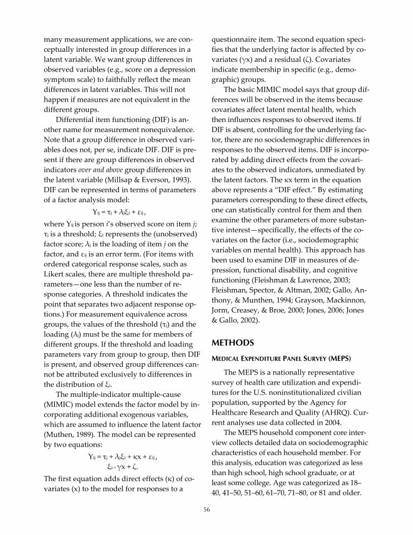
56

many measurement applications, we are con‐ceptually interested in group differences in a latent variable. We want group differences in observed variables (e.g., score on a depression symptom scale) to faithfully reflect the mean differences in latent variables. This will not happen if measures are not equivalent in the different groups.  

Differential item functioning (DIF) is an‐other name for measurement nonequivalence. Note that a group difference in observed vari‐ables does not, per se, indicate DIF. DIF is pre‐sent if there are group differences in observed indicators over and above group differences in the latent variable (Millsap & Everson, 1993). DIF can be represented in terms of parameters of a factor analysis model:     Yij = τj + λjξi + εij ,  where Yij is person i’s observed score on item j; τj is a threshold; ξi represents the (unobserved) factor score; λj is the loading of item j on the factor, and εij is an error term. (For items with ordered categorical response scales, such as Likert scales, there are multiple threshold pa‐rameters—one less than the number of re‐sponse categories. A threshold indicates the point that separates two adjacent response op‐tions.) For measurement equivalence across groups, the values of the threshold (τj) and the loading (λj) must be the same for members of different groups. If the threshold and loading parameters vary from group to group, then DIF is present, and observed group differences can‐not be attributed exclusively to differences in the distribution of ξi. 

The multiple‐indicator multiple‐cause (MIMIC) model extends the factor model by in‐corporating additional exogenous variables, which are assumed to influence the latent factor (Muthen, 1989). The model can be represented by two equations: 

Yij = τj + λjξi + κx + εij , ξi = γx + ζ. 

The first equation adds direct effects (κ) of co‐variates (x) to the model for responses to a 

questionnaire item. The second equation speci‐fies that the underlying factor is affected by co‐variates (γx) and a residual (ζ). Covariates indicate membership in specific (e.g., demo‐graphic) groups. 

The basic MIMIC model says that group dif‐ferences will be observed in the items because covariates affect latent mental health, which then influences responses to observed items. If DIF is absent, controlling for the underlying fac‐tor, there are no sociodemographic differences in responses to the observed items. DIF is incorpo‐rated by adding direct effects from the covari‐ates to the observed indicators, unmediated by the latent factors. The κx term in the equation above represents a “DIF effect.” By estimating parameters corresponding to these direct effects, one can statistically control for them and then examine the other parameters of more substan‐tive interest—specifically, the effects of the co‐variates on the factor (i.e., sociodemographic variables on mental health). This approach has been used to examine DIF in measures of de‐pression, functional disability, and cognitive functioning (Fleishman & Lawrence, 2003; Fleishman, Spector, & Altman, 2002; Gallo, An‐thony, & Munthen, 1994; Grayson, Mackinnon, Jorm, Creasey, & Broe, 2000; Jones, 2006; Jones & Gallo, 2002).  

 METHODS

MEDICAL EXPENDITURE PANEL SURVEY (MEPS)

The MEPS is a nationally representative survey of health care utilization and expendi‐tures for the U.S. noninstitutionalized civilian population, supported by the Agency for Healthcare Research and Quality (AHRQ). Cur‐rent analyses use data collected in 2004.  

The MEPS household component core inter‐view collects detailed data on sociodemographic characteristics of each household member. For this analysis, education was categorized as less than high school, high school graduate, or at least some college. Age was categorized as 18–40, 41–50, 51–60, 61–70, 71–80, or 81 and older. 

57

Race/ethnicity was coded as White (non‐Hispanic), Black (non‐Hispanic), Hispanic, and other. Binary indicators represented these cate‐gories and female gender. 

A self‐administered questionnaire (SAQ) obtained information that could be unreliable if reported by a proxy. For analyzing question‐naire data, special weights were developed in‐corporating adjustments for questionnaire nonresponse (AHRQ, 2002). Ten SAQ items as‐sessed psychological distress, as reflected in feelings of depression or anxiety.  

The questionnaire included Version 2 of the widely used SF‐12 Health Survey (Ware et al., 2002). The mental health subscale comprised two items asking about frequency of feeling “calm and peaceful” and “downhearted and depressed.” The SAQ also included the K6 scale to measure nonspecific psychological distress (Kessler, Barker et al., 2002; Kessler et al., 2003). Using a 30‐day reference period, respondents rated how often they felt “nervous,” “hope‐less,” “restless or fidgety,” “so sad that nothing could cheer you up,” “that everything was an effort,” and “worthless.” The response scale ranged from 4 (all the time) to 0 (none of the time), with higher scores indicating greater distress. The two‐item Patient Health Questionnaire (PHQ‐2), designed as a brief depression screener (Kroenke, Spitzer, & Williams, 2003; Löwe, Kroenke, & Gräfe, 2005), asked “Over the last 2 weeks, how often have you been bothered by any of the following problems?” The prob‐lems were “feeling down, depressed, or hope‐less” and “little interest or pleasure in doing things.” Responses ranged from 0 (not at all) to 3 (nearly every day).   ANALYSES

The analytic sample included those respon‐dents who were eligible to receive the SAQ and completed the questionnaire themselves. The total unweighted sample size for the 2004 MEPS was 34,403 persons, of whom 23,395 were eligible to receive the SAQ. Persons 

younger than 18, institutionalized, or in the military were ineligible for the SAQ. Of those eligible to receive the questionnaire, 93% re‐sponded (n=21,752). Because the SF‐12, K6, and PHQ‐2 may be inaccurate if reported by a proxy, we restricted the analyses to respondents who completed the questionnaires themselves (or with the aid of the interviewer); this reduced the eligible sample to 19,008. A further 47 respon‐dents were removed because they had missing data on all SAQ items, and 188 were excluded due to missing data for education. The final analytic sample included 18,843 respondents. 

For preliminary analyses, we combined the ten items into a summary scale. Because most of the items tap nonspecific psychological distress, we refer to this as the PD scale. We next esti‐mated several MIMIC models using the ten in‐dividual items. The “no‐DIF” model constrained all possible parameters representing DIF effects to equal zero. Models with DIF allowed selected DIF parameters to be freely estimated. The MIMIC model is one kind of structural equation model. We evaluated the fit of no‐DIF and DIF models using several criteria that often are used to evaluate the fit of structural equation models. A goodness‐of‐fit statistic, reflecting the dis‐crepancy between the observed data (item means and covariances) and the model’s pre‐dictions, can be referred to a chi‐square distri‐bution. However, because statistical power increases with sample size, chi‐square good‐ness‐of‐fit tests in large samples should be viewed with caution because trivial differences often appear statistically significant. Conse‐quently, we also examined other indicators of goodness‐of‐fit. The Comparative Fit Index (CFI) and the Tucker‐Lewis Index (TLI) com‐pare the substantive model to a baseline null model of independence among the observed variables; values of 0.95 or higher (with a maximum of 1.0) suggest acceptable fit (Hu & Bentler, 1999). The Root Mean Square Error of Approximation (RMSEA) assesses misfit per degree of freedom; values less than 0.08 suggest 

58

an acceptable fit, while values less than 0.05 suggest very good fit (Browne & Cudek, 1993). 

To determine which of many possible DIF ef‐fects merited closer examination, we examined expected parameter change in the no‐DIF model. The expected parameter change shows the mag‐nitude of change if a previously constrained pa‐rameter is estimated. We focused on values of expected change that exceeded an arbitrary value of 0.05. This situation exemplifies a general issue. When applying structural equation mod‐els to large samples, as are common in national surveys, criteria need to be developed for distin‐guishing which expected changes point to po‐tentially important model modifications and which can be disregarded as minor deviations. 

The MIMIC analyses were conducted using Mplus software (Muthen & Muthen, 1998–2006). Because the items had ordinal response scales with distributions that were not symmet‐ric, weighted least squares estimation was per‐formed based on a polychoric correlation matrix. All analyses incorporated adjustments for the complex sampling design of the MEPS.  RESULTS

Table 1 shows unadjusted mean psychologi‐cal distress scores for different sociodemo‐graphic categories. Women had higher PD scores than men. For education, PD was lower for more highly educated groups. For age, PD was higher for those in the 41–60 age range than for younger people, but PD scores dropped for those between 60–80 years old. Racial/ethnic dif‐ferences in PD were not significant.  MIMIC MODEL RESULTS

A one‐factor confirmatory factor analysis (CFA) model had adequate fit to the data in terms of CFI and TLI (0.965 and 0.992, respec‐tively), but the RMSEA value (0.083) was somewhat high. The residual correlation be‐tween the items “nervous” and “restless” was extremely high. These two items focus more on anxiety symptoms, while the others are more 

oriented to depression. The model was re‐estimated to include this correlation. The re‐vised model had improved fit (CFI = 0.978, TLI = 0.995, RMSEA = 0.065). The factor loadings were all substantial and significant. The lowest load‐ing was for “calm and peaceful” (.321). All sub‐sequent analyses incorporated the residual correlation between “nervous” and “restless.”  

The CFA model was expanded to a MIMIC model by including effects of gender, race/eth‐nicity, education, and age on a latent PD factor. The no‐DIF model did not include direct effects from sociodemographic variables to individual items. Although the chi‐square was significant (χ2 = 1705.15, df = 59), other fit indices were ac‐ceptable (CFI = 0.985, TLI = 0.994, RMSEA = 0.038). If strong DIF effects were present, the no‐DIF model would fit the data poorly. On the basis of these fit indices, one would have some justification for concluding that DIF was not substantially distorting the results. 

Nevertheless, we examined expected pa‐rameter changes to determine where the model could be improved. Three items—“depressed,” 

Table 1. Mean PD Scores, by Demographic Characteristics

CHARACTERISTIC Weighted Proportion

Mean PD Score

Gender Female 0.54 18.40 Male 0.46 15.36

Education < High school 0.17 21.56 High school 0.32 17.18 Some college 0.50 14.86

Race/Ethnicity White 0.71 16.68 Black 0.11 17.62 Hispanic 0.12 17.97 Other 0.06 17.67

Age Group 18–40 0.43 16.73 41–50 0.21 18.13 51–60 0.16 17.93 61–70 0.10 15.10 71–80 0.07 15.48 81+ 0.03 18.07

N=18,190 cases without missing data. Analyses based on weighted data. SOURCE: Center for Financing Access and Cost Trends, AHRQ, MEPS Household Component, 2004.

59

“down,” and “worth”—had no potential DIF effects associated with standardized expected parameter change of 0.05 or higher. These three items constituted an “anchor” without DIF. To identify a model with DIF effects, at least one item (and preferably more) must be assumed to have no DIF. The remaining items had one or more instances of standardized expected pa‐rameter change above 0.05. The “maximal” DIF model included direct effects from all sociode‐mographic variables to each of these latter items, adding a total of 77 parameters to the no‐DIF model (i.e., 7 items times 11 indicators of sociodemographic variables).  

Adding parameters representing DIF effects improved model fit slightly (χ2 = 1596.98, df = 35). The CFI improved marginally (0.986), but the TLI and RMSEA became slightly worse (0.990 and 0.049, respectively), probably due to incorporating a number of direct effects of small magnitude. 

This version of a model incorporating DIF could be considered a maximal adjustment, as all possible DIF effects were included for each nonanchor item. We also estimated a model that included only “major” DIF effects. A major DIF effect was defined as one with a parameter of 0.300 or higher in the DIF model. Again, this criterion represents an arbitrary cutoff, and this is an area in which more methodological work is needed. The fit indices for this “selective” DIF model were CFI = 0.987, TLI = 0.994, RMSEA = 

0.037. The differences in fit between this model and the no‐DIF model were minimal. 

Comparing estimated group differences in models with DIF effects and models without is one method of gauging the impact of DIF. If in‐corporating DIF effects produces substantial changes in the associations of covariates with the factor, then DIF is confounding group dif‐ferences. Table 2 shows the coefficients for the effects of sociodemographic variables on the la‐tent PD factor in the MIMIC models. In this case, the pattern of significant coefficients is similar across the no‐DIF, “maximal” DIF, and “se‐lected” DIF models, although there are slight dif‐ferences in the magnitudes of coefficients. In light of the fact that the no‐DIF model had ac‐ceptable fit, this is not surprising. In the present case, the impact of DIF appears to be minimal.  

Table 3 shows direct effects that were above .300 in absolute value in the “selected” DIF model. It is noteworthy that gender and educa‐tion had no direct effects above this threshold, suggesting an absence of DIF due to these char‐acteristics. DIF as a result of age was concen‐trated in the oldest age groups. It is consistent with common sense to see that people over 70 are more likely to report that everything is an effort, controlling for psychological distress; this is probably a reflection of age‐related dec‐rements in physical capability. For Blacks and Hispanics, some DIF effects were positive and others were negative; this could result in such 

Table 2. Effects of Demographic Variables on Psychological Distress in MIMIC Models VARIABLE No DIF Maximal DIF Selective DIF Female 0.514 (.041)* 0.624 (.050)* 0.574 (.045)* Black –0.065 (.083) –0.020 (.104) –0.078 (.094) Hispanic –0.088 (.061) 0.114 (.077) 0.116 (.075) Other race 0.122 (.095) 0.151 (.114) 0.020 (.110) Age 41–50 0.232 (.064)* 0.325 (.077)* 0.259 (.071)* Age 51–60 0.239 (.066)* 0.364 (.081)* 0.268 (.074)* Age 61–70 –0.274 (.081)* –0.257 (.092)* –0.305 (.090)* Age 71–80 –0.292 (.087)* –0.339 (.100)* –0.437 (.096)* Age 81+ 0.068 (.137) 0.133 (.158) –0.028 (.156) No high school degree 1.046 (.062)* 1.198 (.073)* 1.169 (.069)* High school degree 0.451 (.053)* 0.525 (.064)* 0.505 (.060)* N=18,843. Analyses based on weighted data. Standard errors in parentheses. *Ratio of parameter to standard error exceeds 2.0.

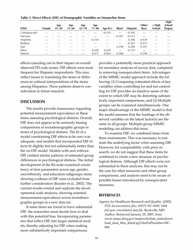
60

effects canceling out in their impact on overall observed PD scale scores. DIF effects were most frequent for Hispanic respondents. This may reflect issues in translating the items or differ‐ences in cultural interpretations of the items among Hispanics. These patterns deserve con‐sideration in future research.  

DISCUSSION

The results provide reassurance regarding potential measurement equivalence in these items assessing psychological distress. Overall, DIF does not appear to be seriously biasing comparisons of sociodemographic groups in terms of psychological distress. The fit of a model constraining DIF effects to be zero was adequate, and models that incorporated DIF ef‐fects fit slightly but not substantially better than the no‐DIF model. Models with and without DIF yielded similar patterns of estimated group differences in psychological distress. The initial development of the K6 scale examined consis‐tency of item parameters across age, gender, race/ethnicity, and education subgroups; items showing evidence of DIF were excluded from further consideration (Kessler et al., 2002). The current results extend and replicate the devel‐opmental scale analyses, showing essential measurement equivalence across sociodemo‐graphic groups in a new data set. 

If some items are found to have substantial DIF, the researcher must decide how to deal with this potential bias. Incorporating parame‐ters that reflect DIF into larger statistical mod‐els, thereby adjusting for DIF when making more substantively important comparisons, 

provides a potentially more practical approach for secondary analyses of survey data, compared to removing nonequivalent items. Advantages of the MIMIC model approach include the fol‐lowing: (1) Comparing estimated effects of key variables when controlling for and not control‐ling for DIF provides an intuitive sense of the extent to which DIF may be distorting substan‐tively important comparisons, and (2) Multiple groups can be examined simultaneously. One major disadvantage of the MIMIC model is that the model assumes that the loadings of the ob‐served variables on the latent factor(s) are the same in all groups. Multiple‐group MIMIC modeling can address this issue. 

To examine DIF, we combined items from three instruments. This was necessary to esti‐mate the underlying factor when assessing DIF. However, for comparability with prior re‐search, we do not suggest that these items be combined to create a new measure of psycho‐logical distress. Although DIF effects were not substantial in these analyses, this may not be the case for other measures and other group comparisons, and analysts need to be aware of possible biases introduced by nonequivalent measures.  REFERENCES

Agency for Healthcare Research and Quality. (2002). PUF documentation files: MEPS HC‐0089, 2004 full‐year consolidated data file. Rockville, MD: Author. Retrieved January 29, 2007, from www.meps.ahrq.gov/mepsweb/data_stats/download_data_files_detail.jsp?cboPufNumber=HC‐089.  

Table 3. Direct Effects (DIF) of Demographic Variables on Nonanchor Items

ITEM Female Age

41–50 Age

51–60 Age

61–70 Age

71–80 Age 81+ Black Hispanic Other Race

< High School

High School Degree

Calm/peaceful — — — — — –0.335 — –0.395 — — — Nervous — — — — — — –0.307 –0.213 — — — Hopeless — — — — –0.218 — — 0.306 0.429 — — Restless — — — — — — — –0.367 0.232 — — Sad — — — — — — 0.290 0.288 0.391 — — Effort — — — — 0.438 0.629 — –0.210 — — — Interest — — — — 0.473 0.463 0.360 — 0.349 — —

61

Browne, M. W., & Cudeck, R. (1993). Alternative ways of assessing model fit. In K. A. Bollen & J. S. Long (Eds.), Testing structural equation models (pp 136–162). Thousand Oaks, CA: Sage. 

Burdine, J. N., Felix, M., Abel, A., Wiltraut, C., & Musselman, Y. (2000). The SF‐12 as a population health measure: An exploratory examination of potential for application. Health Services Research, 35, 885–904. 

Fleishman, J. A., & Lawrence, W. F. (2003). Demo‐graphic variation in SF‐12 scores: True differ‐ences or differential item functioning. Medical Care, 41, III‐75–III‐86. 

Fleishman, J. A., Spector, W. D., & Altman, B. M. (2002). Impact of differential item functioning on age and gender differences in functional disabil‐ity. Journals of Gerontology: Social Sciences, 57(B), S275–S284. 

Gallo, J. J., Anthony, J. C., & Muthen, B. O. (1994). Age differences in the symptoms of depression: A latent trait analysis. Journals of Gerontology: Psychological Sciences, 49, P251–P264. 

Grayson, D. A., Mackinnon, A., Jorm, A. F., Creasey, H., & Broe, G. A. (2000). Item bias in the Center for Epidemiologic Studies Depression Scale: Ef‐fects of physical disorders and disability in an elderly community sample. Journals of Gerontol‐ogy: Psychological Sciences, 55B, P273–P282. 

Hu, L. T., & Bentler, P. M. (1999). Cutoff criteria for fit indexes in covariance structure analysis: Conventional criteria versus new alternatives. Structural Equation Modeling, 6, 1. 

Jones, R. N. (2006). Identification of measurement differences between English and Spanish lan‐guage versions of the Mini‐Mental State Exami‐nation: Detecting differential item functioning using MIMIC modeling. Medical Care, 44, S124–S133. 

Jones, R. N., & Gallo, J. J. (2002). Education and sex differences in the Mini‐Mental State Examina‐tion: Effects of differential item functioning. Journals of Gerontology: Psychological Sciences, 57B, P548–P558. 

Kessler, R. C., Andrews, G., Colpe, L. J., Hiripi, E., Mroczek, D. K., Normand, S.‐L. T., et al. (2002). 

Short screening scales to monitor population prevalences and trends in non‐specific psycho‐logical distress. Psychological Medicine, 32, 959–976. 

Kessler, R. C., Barker, P. R., Colpe, L. J., Epstein, J. F., Gfroerer, J. C., Hiripi, E., et al. (2003). Screening for serious mental illness in the general popula‐tion. Archives of General Psychiatry, 60, 184–189. 

Kessler, R. C., Berglund, P., Demler, O., Jin, R., Ko‐retz, D., Merikangas, K. R., et al. (2003). The epi‐demiology of major depressive disorder: Results from the National Comorbidity Survey Replica‐tion (NCS‐R). Journal of the American Medical As‐sociation, 289, 3095–3105. 

Kessler, R. C., & Zhao, S. (1999). Overview of de‐scriptive epidemiology of mental disorders. In C. S. Aneshensel & J. Phelan (Eds.), Handbook of the sociology of mental health. New York: Kluwer Academic/Plenum. 

Kroenke, K., Spitzer, R. L., & Williams, J. B. W. (2003). The Patient Health Questionnaire‐2: Va‐lidity of a two‐item depression screener. Medical Care, 41, 1284–1292. 

Löwe, B., Kroenke, K., & Gräfe, K. (2005). Detecting and monitoring depression with a two‐item questionnaire (PHQ‐2). Journal of Psychosomatic Research, 58, 163–171. 

Millsap, R. E., & Everson, H. T. (1993). Methodology review: Statistical approaches for assessing measurement bias. Applied Psychological Meas‐urement, 17, 297. 

Muthen, B. O. (1989). Latent variable modeling in heterogeneous populations. Psychometrika, 54, 557–585. 

Muthen, L. K., & Muthen, B. O. (1998–2006). Mplus user’s guide (4th ed.). Los Angeles: Muthen and Muthen. 

Radloff, L. S. (1977). The CES‐D Scale: A self‐report depression scale for research in the general population. Applied Psychological Measurement, 1, 395–401. 

Ware, J. E., Kosinski, M., Turner‐Bowker, D. M., & Gandek, B. (2002). SF‐12v2: How to score Version 2 of the SF‐12 Health Survey. Lincoln, RI: Quality‐Metric, Inc. 

 

63

FEATURE PAPER: Reliability and Validity of a Colorectal Cancer Screening (CRCS) Questionnaire by Mode of Survey Administration

Sally W. Vernon, University of Texas–Houston Jasmin A. Tiro, National Cancer Institute

Rachel W. Vojvodic, Sharon P. Coan, and Pamela M. Diamond, University of Texas–Houston Anthony Greisinger, Kelsey Research Foundation

  INTRODUCTION

Valid and reliable self‐report measures of cancer screening behaviors are important for (1) identifying correlates and predictors of behav‐ior, (2) evaluating the effectiveness of behav‐ioral interventions, and (3) monitoring progress and trends in adherence to cancer screening guidelines (Hiatt, Klabunde, Breen, Swan, & Ballard‐Barbash, 2002; Vernon, Briss, Tiro, & Warnecke, 2004). The implementation of federal legislation limiting access to medical records (Health Insurance Portability and Accountabil‐ity Act of 1996 [HIPAA]) is likely to increase the need to use self‐reported data in epidemiologic, health services, and behavioral research studies. For colorectal cancer screening (CRCS), assess‐ing the accuracy of self‐reports is especially dif‐ficult because there are multiple types of acceptable screening tests (i.e., fecal occult blood test [FOBT], sigmoidoscopy [SIG], colonoscopy [COL], and barium enema [BE]), the recommended time interval for test comple‐tion differs within and between tests, and the guidelines have changed over time (Vernon et al., 2004). Adding to this complexity is the number of measures of utilization (e.g., initial, recent, regular, ever).  

Survey items measuring CRCS on the Na‐tional Health Interview Survey (NHIS) and the Behavioral Risk Factor Surveillance System (BRFSS) have differed over time and between surveys. There is one test‐retest reliability study on CRCS for the BRFSS (Bradbury, Brooks, Brawarsky, & Mucci, 2005), but we know of no studies validating CRCS questions used in these national surveys. Yet these measures fre‐quently are adapted by investigators conduct‐ing descriptive and intervention studies.  

In 1999, the National Cancer Institute (NCI) convened a group of experts to develop uni‐form definitions and measures to assess CRCS behaviors (hereafter called the NCI CRCS ques‐tionnaire) (Vernon, Meissner et al., 2004). The initial draft of the NCI CRCS questionnaire un‐derwent cognitive testing as part of the devel‐opment of NCI’s Health Information National Trends Survey in 2003. Qualitative data from focus groups (Bastani, Gallardo, & Maxwell, 2001; Beeker, Kraft, Southwell, & Jorgensen, 2000; Goel et al., 2004; Weitzman, Zapka, Es‐tabrook, & Goins, 2001) showed that many adults do not know or recognize the names of CRCS tests and that many were unable to dis‐tinguish between SIG and COL or between home‐based and office‐based FOBT (Baier et al., 2000; Madlensky, McLaughlin, & Goel, 2003); therefore, the cognitive interviews focused on issues related to comprehension and interpreta‐tion of the questions and, to a lesser extent, on strategies respondents used to recall informa‐tion. Findings from the cognitive interviews were consistent with previous data and led to a revised questionnaire and a recommendation that CRCS test descriptions be provided prior to asking questions about test use (Vernon, Meissner et al., 2004).  

The purpose of the research described in this report was to evaluate the reliability and validity of three of the screening tests included in the NCI CRCS questionnaire: FOBT, SIG, and COL. A secondary objective was to determine if validity estimates are equivalent across three modes of administration (mail, telephone, and face‐to‐face). We focused on mode of admini‐stration because mode differences might affect comparisons of estimates from national surveys 

64

(NHIS is administered face‐to‐face, while BRFSS is administered over the telephone). We also evaluated, with a subsample, the test‐retest reliability of the NCI CRCS questionnaire over a two‐week time period.   METHODS STUDY POPULATION

This study was approved by the University of Texas Health Science Center at Houston Committee for the Protection of Human Sub‐jects (HSC‐SPH‐04‐111). The target population was men and women between 51 and 74 years of age who had received primary care at the Kelsey‐Seybold Clinic (KSC) in Houston, Texas, for at least five years prior to being invited to participate in the study. We selected a relatively homogeneous and stable patient population in a setting with strong medical record and auxil‐iary data systems. Patients were excluded if they had a history of colorectal cancer. Eligibil‐ity status was determined from the KSC elec‐tronic administrative database and was verified at the time of study enrollment.  

We used a case‐control study design to maximize efficiency. Cases were defined as KSC patients who had a recent home FOBT, SIG, or COL recorded in the administrative da‐tabase. We followed 2007 American Cancer So‐ciety (ACS) guidelines to define recency: a FOBT within the past year, or a SIG or COL within the past five years. We limited our defi‐nition of “recent COL” to the past five years be‐cause a COL received prior to becoming a KSC patient may not have been recorded in the da‐tabase. Controls either never had a CRCS test or no recent CRCS test was recorded in the KSC database. Cases could have a single CRCS test or multiple tests and, therefore, could serve as a case or a control for each CRCS test type. If the case had multiple tests of a particular type (e.g., two SIGs), we used the most recent test in the database. Our goal is to collect self‐report data on 200 cases and 100 controls per mode of ad‐ministration (mail, telephone, and face‐to‐face) 

with at least 100 cases for each CRCS type across all modes. At the time of this report, we had collected data for the validation study from 385 cases and 201 controls. 

 RECRUITMENT

Eligible cases and controls were randomly selected from the KSC database every two weeks and were mailed invitation letters de‐scribing the study and containing contact in‐formation for the Kelsey Research Foundation (KRF). Study candidates were told they could decline participation by calling the KRF; those who did not actively decline participation were called by a KRF research assistant after mailing the invitation letter. During the call, the re‐cruiter ascertained eligibility, obtained verbal HIPAA and informed consent, and obtained consent to review the participant’s medical re‐cord. Candidates were called at least six times before being classified as a nonrespondent. Pa‐tients who refused to participate were asked why they declined.   QUESTIONNAIRE

We modified the format of the NCI CRCS questionnaire for mail, telephone, and face‐to‐face administration. We developed two ver‐sions of the questionnaire, one to be mailed with explicit instructions and detailed skip pat‐terns, and the other to be used for telephone and face‐to‐face interviews with interviewer scripts and prompts. Both versions were pro‐fessionally printed as eight‐page color booklets that were also scannable.  

Pilot testing of the mail and telephone ver‐sions of the questionnaire revealed that people were confused by the order and skip patterns of the first four questions for each CRCS test. As a result, we reordered the questions to help re‐spondents identify and follow the skip pattern appropriate for their CRCS test history. 

For each CRCS test, respondents were asked if they ever had the test, whether they had ever heard of the test, whether their physician rec‐ommended the test, the time interval of the 

65

most recent test, the month and year of the most recent test, and whether the most recent test was done at a KSC facility. We also in‐cluded questions about sociodemographics (sex, age, marital status, race, ethnicity, educa‐tion), use of the health care system (recency of last KSC visit, number of KSC and non‐KSC visits during the past five years), family history of CRC, and social desirability. To assess social desirability, we used a short ten‐question ver‐sion of the Marlowe‐Crowne Social Desirability Scale (Strahan & Gerbasi, 1972).  SURVEY ADMINISTRATION

Every week, names of new enrollees were sent from the KRF to project staff at the Univer‐sity of Texas to be randomized to survey ad‐ministration mode, and a subset of those was selected for the test‐retest reliability study. We followed the Dillman approach for mail sur‐veys (Dillman, 1978). Enrollees randomized to the mail mode received a packet consisting of a letter reiterating their agreement to participate in the study, a standardized bubble‐formatted questionnaire, a postage‐paid envelope, and a pencil. Nonrespondents were mailed a second packet after four weeks and a final reminder postcard after eight weeks. Sixteen weeks from the enrollment date, enrollees who did not re‐turn a mail questionnaire were classified as dropouts. Enrollees randomized to the face‐to‐face mode were called to set up a time for an interview to be conducted at the participant’s home or at the centrally located KSC main campus, depending on the preference of the study participant. Almost two‐thirds of face‐to‐face participants (61%) chose to have their in‐terview conducted at their homes. Enrollees randomized to the telephone and face‐to‐face modes were called at least six times before be‐ing classified as dropouts. If possible, messages were left requesting that the enrollee call the project’s local telephone number. Participants were mailed a $20 honorarium after completing the questionnaire.  

RELIABILITY STUDY

A subset of enrollees who completed the questionnaire was randomly selected to com‐plete a second survey to evaluate test‐retest re‐liability. They were randomly assigned to one of three time intervals (two weeks, three months, or six months). Our goal is to complete 65 reliability surveys for each time interval per mode of administration (total n = 585). The same survey administration protocols were fol‐lowed for each mode. After completing the sec‐ond survey, participants were mailed another $20 honorarium. At the time of this report, reli‐ability results were available only for the two‐week follow‐up (n = 179).   MEDICAL RECORD ABSTRACTION

We chose to combine data from the medical record and the electronic administrative data‐base as our gold standard (hereafter referred to as the combined medical record). Recent stud‐ies have described sources of measurement er‐ror in both data sources, such as failing to include laboratory reports, delayed recording, and incomplete recordkeeping in public health care settings (Fiscella, Holt, Meldrum, & Franks, 2006; Peabody, Luck, Glassman, Dresselhaus, & Lee, 2000). Data from the electronic administra‐tive database and medical record abstractions were merged, and duplicates were deleted. Pri‐ority was given to the administrative records for any conflicts in test type or date. We ab‐stracted the following information for all CRCS tests: date of first and most recent patient visit, KSC or non‐KSC test facility (if applicable), test date, reason, results, and outcome, including where these data were found.   STATISTICAL ANALYSIS

We used chi‐square statistics to determine if sociodemographic and health care use differed among cases and controls. For social desirabil‐ity, we used an ANOVA to see if response ten‐dencies differed by mode of administration.  

 

66

Validity Analysis

For each screening test (FOBT, SIG, and COL), we compared a participant’s self‐report to his/her combined medical record. Both self‐reported screening behavior and actual screen‐ing behavior were defined in terms of compli‐ance with 2007 ACS guidelines. We calculated time from the most recent exam to the survey completion date for both self‐report and medical record. For each screening test, validity was evaluated with four summary measures: con‐cordance, sensitivity, specificity, and report‐to‐records ratio. We calculated two‐sided 95% con‐fidence intervals for all four measures. Estimates were calculated for each CRCS test across all modes of administration as well as stratified by mode of administration. We used Tisnado et al.’s (2006) criteria, where concordance, sensitivity, and specificity values > 0.9 indicated excellent agreement between a patient’s self‐report and the medical record and values > 0.8 indicated good agreement. Very few published studies of validity report CIs for sensitivity and specificity, and there are no published criteria for what is acceptable precision. We judged a measure to have good precision if the lower bound of the confidence limit was 0.80 or greater.  

 Reliability Analysis

We calculated the raw agreement between the initial and two‐week surveys for receipt of each CRCS test within guidelines. We also cal‐culated kappa statistics and 95% confidence in‐tervals to correct for chance agreement. According to Landis and Koch (1977), kappa values between 0.61 and 0.79 indicate substan‐tial agreement, and values greater than or equal to 0.80 indicate almost perfect agreement.  RESULTS

From September 2005 to December 2006, we invited 4,541 potential study candidates. We contacted 3,028 (67%), and the remaining 1,513 (33%) were not contacted because they could not be reached within the call limit (n = 370), 

had invalid contact information (n = 103), were deceased (n = 18), or were not needed because we had filled our sample (n = 1,022). Of the 3,028 we contacted, we lost 861 (28%) to follow‐up either because they were unable to partici‐pate due to illness (n = 70) or were ineligible (n = 791). Of the remaining contacted (n = 2,167), 870 (40%) were enrolled, 99 (5%) dropped out after enrollment, and 1,198 (55%) refused. 

As of January 26, 2007, we had completed data collection with 586 of the 870 enrollees. The case‐control distribution was 201 controls (e.g., never or no recent CRCS test), 254 cases with a single CRCS test within guidelines, and 131 cases with multiple CRCS tests within guidelines.  

There were no significant sociodemographic differences between cases and controls except for marital status (78% of cases were married compared with 70% of controls). The majority of cases and controls were less than 65 years old, female, non‐Hispanic, Caucasian, and had some college or a college degree. Almost all cases and controls had visited a physician in the past year (96% and 92%, respectively), and all had visited a physician in the past two years. Cases were significantly more likely than con‐trols to report physician recommendation of FOBT (50% vs. 22%) and SIG (82% vs. 48%) but not COL (56% vs. 53%). Average scores for the Marlowe‐Crowne social desirability scale were significantly higher for respondents completing the face‐to‐face survey (mean = 6.08, SD = 1.48) compared with the mail survey (mean = 5.59, SD = 1.48). Scores for the telephone survey were intermediate (mean = 5.77, SD = 1.49).1   VALIDITY

Overall concordance estimates for FOBT, SIG, and COL self‐reports met our criteria for good agreement—the concordance estimate was > 0.80, and the lower confidence limit did not fall below 0.80 (Table 1). Estimates of con‐cordance by mode of administration showed no 

1 ANOVA results: F(2, 583) = 5.22, p = 0.0057. 

67

significant mode differences within each CRCS test type—i.e., the CIs overlapped; however, the lower bound of the CI was below 0.80 for about half of the estimates.  

The overall sensitivity estimate for COL was good, but estimates for FOBT and SIG did not meet the criterion that the lower bound of the CI be at least 0.80, and for SIG, the point estimate was below 0.80 (Table 1). Sensitivity estimates also varied by mode of administration. For FOBT, the sensitivity estimate for respondents completing the mailed survey was less than 0.80 and was lower compared with those completing telephone and face‐to‐face interviews, although the CIs overlapped (Table 1). The reverse was true for COL self‐reports, where sensitivity was higher for mail respondents, although, again, the CIs overlapped. There was no apparent differ‐ence by mode for SIG self‐reports. The CIs for all of the sensitivity estimates were wider than those for concordance and specificity.  

Overall estimates of specificity met our cri‐teria for acceptability (Table 1). All specificity estimates by mode of administration also were greater than 0.80; however, for SIG and FOBT, the lower bound of the CI was slightly below 0.80.  

The overall report‐to‐records ratios indicated over‐reporting for FOBT and COL but not for SIG (Table). These patterns were consistent across mode for each of the tests although the CIs were wide.   RELIABILITY

The raw agreement between the initial and two‐week reliability surveys was over 87% for FOBT, 89% for SIG, and 95% for COL. Kappa statistics for FOBT (k = 0.71, 95% CI: 0.70–0.73) and SIG (k = 0.73, 95% CI: 0.72–0.74) indicated substantial agreement between initial and sec‐ond surveys based on Landis and Koch’s (1977) 

Table 1. Measures of Agreement (Concordance, Sensitivity, Specificity, & Report-to-Records Ratio) between Self-Reports & the Combined Medical Record, by CRCS Test Type & Mode of Survey Administration for Patients Attending a Primary Care Clinic in Houston, Texas (n = 586) FOBT* SIG* COL* n Concordance 95% CI n Concordance 95% CI n Concordance 95% CI Overall 586 0.84 (0.81–0.88) 586 0.84 (0.81–0.87) 586 0.88 (0.86–0.91) Mode

Mail 197 0.84 (0.78–0.89) 197 0.85 (0.80–0.91) 197 0.89 (0.84–0.93) Telephone 207 0.85 (0.80–0.90) 207 0.85 (0.79–0.90) 207 0.88 (0.84–0.93) Face-to-face 182 0.84 (0.78–0.90) 182 0.82 (0.76–0.89) 182 0.88 (0.83–0.93)

n Sensitivity 95% CI n Sensitivity 95% CI n Sensitivity 95% CI Overall 134 0.81 (0.74–0.89) 183 0.77 (0.70–0.84) 139 0.91 (0.86–0.96) Mode

Mail 44 0.73 (0.57–0.88) 62 0.77 (0.66–0.89) 43 0.95 (0.89–1.00) Telephone 61 0.87 (0.78–0.96) 57 0.75 (0.64–0.88) 56 0.89 (0.81–0.98) Face-to-face 29 0.83 (0.68–0.98) 64 0.78 (0.67–0.90) 40 0.90 (0.80–1.00)

n Specificity 95% CI n Specificity 95% CI n Specificity 95% CI Overall 452 0.85 (0.82–0.89) 403 0.87 (0.84–0.91) 447 0.87 (0.84–0.91) Mode

Mail 153 0.87 (0.81–0.93) 135 0.89 (0.83–0.95) 154 0.87 (0.81–0.93) Telephone 146 0.84 (0.78–0.91) 150 0.88 (0.82–0.94) 151 0.88 (0.83–0.94) Face-to-face 153 0.84 (0.78–0.91) 118 0.85 (0.78–0.92) 142 0.87 (0.81–0.93)

Report to Records Ratio** Report to Records Ratio** Report to Records Ratio** Overall 1.31 (1.15–1.47) 1.05 (0.94–1.16) 1.32 (1.18–1.45) Mode

Mail 1.18 (0.91–1.46) 1.02 (0.84–1.19) 1.42 (1.16–1.68) Telephone 1.25 (1.04–1.45) 1.07 (0.87–1.27) 1.21 (1.02–1.40) Face-to-face 1.66 (1.18–2.13) 1.06 (0.88–1.24) 1.35 (1.08–1.62)

* Compliance with guidelines is defined as an annual FOBT or a SIG or COL within five years. ** Report-to-records ratio is a measure of net bias in test reporting with values greater than 1.0 indicating over-reporting and values less than 1.0 indicating under-reporting.

68

criteria. For COL, the agreement was almost perfect (k = 0.89, 95% CI: 0.88–0.91).   DISCUSSION

Our findings compare favorably with past validity studies that assessed recent FOBT, SIG, and COL self‐reports. The NCI CRCS question‐naire items assessing recency of FOBT, SIG, and COL achieved acceptable levels of concordance, specificity, and two‐week test‐retest reliability. General levels of raw agreement for each CRCS test type with the medical record were above 80%, and patients were able to accurately recall not having a particular CRCS test. We could not directly compare our test‐retest reliability with Bradbury et al.’s findings (2005) because we used different prevalence definitions (e.g., FOBT in the past year vs. ever had FOBT) and different time intervals between surveys (e.g., Bradbury and colleagues’ mean time interval was 77 days).  

The sensitivity estimate for recent COL was good to excellent, with 91% of respondents ac‐curately recalling having had the test, while sensitivity estimates for questions about the most recent FOBT and SIG were not as good, probably due to small numbers. In other words, patients had a harder time recalling whether they had had an FOBT in the past year or a SIG in the past five years.  

The differences in recall across CRCS test types may be due to test characteristics. Some researchers have suggested that COL may be more memorable to patients because they were sedated, needed to arrange for transport from the procedure, and needed to take a full day off from work. For SIG, in particular, patients may be confusing this test type with COL. In other words, people may not recall the name of the test and falsely label it a COL. COL has re‐ceived more attention from the media, and so it may have more name recognition. Alterna‐tively, patients may believe COL is a superior screening test and, therefore, may want to recall that they had the “better” test (Meissner, Breen, 

Klabunde, & Vernon, 2006). This finding may also account for the higher report‐to‐records ra‐tio—i.e., overreporting—found for COL. For FOBT, a possible reason for lower sensitivity may be recall bias with respect to time period. Patients may recall receipt of an FOBT as hap‐pening more recently than it did. We are cur‐rently investigating whether a 15‐month time window increases sensitivity; however, Tisnado et al.’s (2006) findings suggest that variations in the time window do not substantially alter con‐cordance.  

Our response rate of 40% may introduce re‐sponse bias, but the direction and magnitude of any potential bias is unclear. Recent methodo‐logical research suggests that lower response rates do not necessarily indicate larger biases in survey estimates (Keeter, Miller, Kohut, Groves, & Presser, 2000; Tourangeau, 2004). Another potential limitation of our study is that the find‐ings may not generalize to other health care set‐tings, such as community clinics. We chose to conduct the study in a clinic setting with a rela‐tively stable patient population where the medical records and administrative data sources were likely to be accurate and com‐plete. Thus, our estimates probably represent a “best case” scenario. 

 CONCLUSION

Valid and reliable self‐report measures are a critical component of CRC prevention and con‐trol research. This study provides empirical support for the use of the NCI CRCS question‐naire to assess prevalence of recent behavior. Intervention researchers using the question‐naire to assess CRCS prevalence should weigh their selection of mode of administration against their research objectives (i.e., whether it is more important to reduce false positives or false negatives) and the characteristics of their target population. Future research should in‐vestigate the performance of the NCI CRCS questionnaire in different health care settings.   

69

REFERENCES

American Cancer Society. (2007). Cancer facts and fig‐ures, 2007. Atlanta: Author. 

Baier, M., Calonge, B. N., Cutter, G. R., McClatchey, M. W., Schoentgen, S., Hines, S., et al. (2000). Va‐lidity of self‐reported colorectal cancer screening behavior. Cancer Epidemiology, Biomarkers & Pre‐vention, 9, 229–232. 

Bastani, R., Gallardo, N. V., & Maxwell, A. E. (2001). Barriers to colorectal cancer screening among ethnically diverse high‐ and average‐risk indi‐viduals. Journal of Psychosocial Oncology, 19, 65–84. 

Beeker, C., Kraft, J. M., Southwell, B. G., & Jorgen‐sen, C. M. (2000). Colorectal cancer screening in older men and women: Qualitative research findings and implications for intervention. Jour‐nal of Community Health, 25, 263–277. 

Bradbury, B. D., Brooks, D. R., Brawarsky, P., & Mucci, L. A. (2005). Test‐retest reliability of colo‐rectal testing questions on the Massachusetts Behavioral Risk Factor Surveillance System (BRFSS). Preventive Medicine, 41, 303–311. 

Dillman, D. A. (1978). Mail and telephone surveys: The total design method. New York: John Wiley & Sons. 

Fiscella, K., Holt, K., Meldrum, S., & Franks, P. (2006). Disparities in preventive procedures: Comparisons of self‐report and Medicare claims data. BioMed Central Health Services Research, 6, 1–8. 

Goel, V., Gray, R. E., Chart, P. L., Fitch, M., Saibil, F., & Zdanowicz, Y. (2004). Perspectives on colorec‐tal cancer screening: A focus group study. Health Expectations, 7, 51–60. 

Hiatt, R. A., Klabunde, C. N., Breen, N. L., Swan, J., & Ballard‐Barbash, R. (2002). Cancer screening practices from National Health Interview Sur‐veys: Past, present, and future. Journal of the Na‐tional Cancer Institute, 94, 1837–1846. 

Keeter, S., Miller, C., Kohut, A., Groves, R. M., & Presser, S. (2000). Consequences of reducing nonresponse in a national telephone suvey. Pub‐lic Opinion Quarterly, 64, 125–148. 

Landis, J. R., & Koch, G. G. (1977). The measurement of observer agreement for categorical data. Bio‐metrics, 33, 159–174. 

Madlensky, L., McLaughlin, J. R., & Goel, V. (2003). A comparison of self‐reported colorectal cancer screening with medical records. Cancer Epidemi‐ology, Biomarkers & Prevention, 12, 656–659. 

Meissner, H. I., Breen, N. L., Klabunde, C. N., & Vernon, S. W. (2006). Patterns of colorectal can‐cer screening uptake among men and women in the US. Cancer Epidemiology, Biomarkers & Preven‐tion, 15, 389–394. 

Peabody, J. W., Luck, J., Glassman, P., Dresselhaus, T. R., & Lee, M. (2000). Comparison of vignettes, standardized patients, and chart abstraction: A prospective validation study of 3 methods for measuring quality. Journal of the American Medi‐cal Association, 283, 1715–1722. 

Strahan, R., & Gerbasi, K. C. (1972). Short, homoge‐neous versions of the Marlowe‐Crowne Social Desirability Scale. Journal of Clinical Psychology, 28, 191–193. 

Tisnado, D. M., Adams, J. L., Liu, H., Damberg, C. L., Chen, W.‐P., Hu, F. A., et al. (2006). What is the concordance between the medical record and patient self‐report as data sources for ambu‐latory care? Medical Care, 44, 132–140. 

Tourangeau, R. (2004). Survey research and societal change. Annual Review of Psychology, 55, 775–801. 

Vernon, S. W., Briss, P. A., Tiro, J. A., & Warnecke, R. B. (2004). Some methodologic lessons learned from cancer screening research. Cancer, 101, 1131–1145. 

Vernon, S. W., Meissner, H. I., Klabunde, C. N., Rimer, B. K., Ahnen, D., Bastani, R., et al. (2004). Measures for ascertaining use of colorectal can‐cer screening in behavioral, health services, and epidemiologic research. Cancer Epidemiology, Biomarkers & Prevention, 13, 898–905. 

Weitzman, E. R., Zapka, J. G., Estabrook, B., & Goins, K. V. (2001). Risk and reluctance: Under‐standing impediments to colorectal screening. Preventive Medicine, 32, 502–513.

  

 

71

FEATURE PAPER: Reliability and Data Quality in the National Survey on Drug Use and Health

Joel Kennet, Joe Gfroerer, and Peggy Barker, Substance Abuse and Mental Health Services Administration

Lanny Piper, Erica Hirsch, Becky Granger, and James R. Chromy, RTI International  

 INTRODUCTION

Information on data quality should be a standard output of major federal surveys, as these data can influence major policy decisions. Most surveys dutifully report on response rates and sampling error, but not on measurement er‐ror. Response rates, which can indicate potential sources of bias in data, cannot truly measure data accuracy. Re‐interviewing respondents provides a direct measure of response variance. In other words, the capability of the survey to provide accurate data and consequent popula‐tion estimates can be determined by assessing its reliability. Reliability is of particular concern when respondents are asked questions on sensi‐tive topics. In addition, when particular popula‐tion subgroups yield different estimates of reliability, concerns may be raised regarding the cultural competency of the survey instrument and the validity of conclusions about health dis‐parities (Johnson & Bowman, 2003). 

A few surveys on substance use have car‐ried out test‐retest reliability studies in the past and have reported differential response consis‐tency across racial groups (Shea, Stein, Lanti‐gua, & Basch, 1991; Stein, Lederman, & Shea, 1993; Stein, Courval, Lederman, & Shea, 1995; Johnson & Mott, 2001). With the exception of the Johnson and Mott study, these have been carried out on state and local samples or have had other limitations with respect to their abil‐ity to produce generalizable results. While con‐ducted on a national sample (NLSY), the Johnson and Mott study produced results that were contradicted in another study using more recent waves of data (Shillington & Clapp, 2000). An additional consideration is that none of the surveys analyzed for reliability used au‐

dio computer‐assisted self‐interview (ACASI) administration, which seems likely to enhance response consistency.  

The National Survey on Drug Use and Health (NSDUH) is an annual cross‐sectional household survey of the civilian, noninstitu‐tionalized U.S. population age 12 and older. The survey gathers data on the recency and fre‐quency of use of alcohol, tobacco, and illicit substances from a probability sample of ap‐proximately 67,500 respondents selected each year in all 50 states and the District of Columbia. Recognizing that illicit drug use is a sensitive topic, the NSDUH uses state‐of‐the‐art methods to assure respondents of their privacy and con‐fidentiality in providing truthful data. The ma‐jority of the survey is administered in ACASI mode so that no persons other than respondents are able to see the answers provided. Further, NSDUH staff have taken many steps to assure that the questionnaire and other survey instru‐ments are understandable to a broad cross‐section of the population. New items undergo extensive expert review and cognitive testing, and the full questionnaire receives periodic re‐views for readability. While several studies have been done to assess the validity of self‐reported drug use in NSDUH, its test‐retest re‐liability has never been studied before. 

In an effort to assess the reliability of NSDUH data, a study was carried out during April–December 2006, wherein a subset of re‐spondents participated in a reliability study. We refer to reliability as the extent to which re‐spondents answered alike when the same ques‐tions were presented on two occasions separated by a specified time period.  

High reliability is a necessary condition that must be met for data to be considered valid. If a 

72

question or set of questions proves unreliable, either within a particular population subgroup or overall, then discussion of disparities in the construct purportedly being measured loses its grounding. For example, if the overall reliability of the NSDUH measure of depression was found to be good but its reliability among a specific subpopulation was poor, then any disparity in depression prevalence between the specific sub‐population and others might simply be an arti‐fact resulting from measurement error.  

At the time of this writing, reliability study data obtained in the fourth quarter of 2006 are being cleaned and processed for inclusion in the final data set. Therefore, this paper will de‐scribe only results obtained using the responses from the second and third quarters of 2006. Re‐sults from the full reliability study are expected to become available in late 2007. Data from ap‐proximately 2,200 NSDUH respondents are in‐cluded in the present analyses. The full data set will contain approximately 3,100 paired inter‐view records. When analyses are complete, it is expected that the study will reveal which NSDUH measures are most at risk of producing unreliable estimates, and which population subgroups might tend to produce reliability scores that differ from others.  METHODS  PARTICIPANTS

The reliability study sample was drawn from the NSDUH main sample. For practical reasons, respondents in Alaska and Hawaii were not included in the reliability study, nor were non‐English speaking respondents in any state, although Spanish‐speaking respondents are included in the main sample. In addition, as a precaution against contamination of the data, the reliability study did not include respon‐dents in households in which more than one person was selected to participate in the survey. Table 1 shows the demographic characteristics of the sample based on the first interview. 

 MATERIALS & PROCEDURE

The materials and procedures used in the re‐liability study were nearly identical to those used in the 2006 NSDUH main study (for de‐tailed descriptions see SAMHSA, 2005, and the Methodological Resource Book on the SAMHSA Web site). To summarize, potential respondent households received a letter that briefly de‐scribed the survey and encouraged participation. Interviewers arrived at these households within several days and attempted to administer the screener using a hand‐held computer. After be‐ing selected and agreeing to participate, respon‐dents answered a few demographic questions verbally and then began the ACASI portion of the survey. Interviews were administered as 

Table 1. Sample Composition CHARACTERISTIC N TOTAL 2,204 Age

12–17 695 18–25 684 26 or older 825

Race/Ethnicity White, not Hispanic 1,511 Black, not Hispanic 312 Other, not Hispanic 148 Hispanic 225

Gender Male 994 Female 1,210

Family Income $24,999 or less 550 $25,000–$49,999 617 $50,000–$74,999 326 $75,000–$99,999 207 $100,000 or more 253

Country of Birth U.S. born 2,068 Foreign born 136

County Type Metropolitan 1,783 Nonmetropolitan 421

Health Insurance Covered 1,849 Not covered 342

Education Less than high school 102 High school diploma 251 Some college 214 College graduate 258

Source: SAMHSA, Office of Applied Studies, National Survey on Drug Use and Health, Q2 & Q3 of 2006.

73

privately as was practical, and headphones were used to assure privacy. After completing the ACASI section, the interviewer retrieved the computer and asked a series of demographic questions, which were read aloud by the inter‐viewer from the computer screen. Finally, the interviewer thanked the respondent and paid a $30 incentive. At this point, if a respondent was selected for the reliability study, additional screens would appear on the laptop, which the interviewer would read in an attempt to recruit the respondent for an additional study, the purpose of which was to “help us improve our interviewing procedures and how we ask ques‐tions.” Neither respondents nor interviewers were aware beforehand that there would be an opportunity for a second interview. A $50 in‐centive was offered for the re‐interview, which was scheduled to be administered 5–15 days later. An additional manipulation was whether the same interviewer or a different one would return for the second interview. The analyses in this paper will report on data pooled over these two conditions.   DEMOGRAPHIC VARIABLES

Demographic variables used in the tables are based on the first interview conducted with each respondent. No effort was made to resolve any differences with the re‐interview demo‐graphic classifications or to assess their reliabil‐ity. For the purposes of this paper, they are used simply to define subpopulation groups of interest for the evaluation of reliability of the outcome variables discussed below.   OUTCOME VARIABLES Lifetime Substance Use 

The NSDUH ACASI section asks about re‐spondents’ experiences with a wide variety of illicit drugs, alcohol, and tobacco. This analysis is limited to use of cigarettes, alcohol, mari‐juana, and nonmedical use of prescription drugs. Similar to other preliminary analyses in NSDUH done using raw substance use vari‐

ables, respondents with missing data for a par‐ticular substance were considered not to have used that substance.  Past-Year Substance Use 

Positive responders to the lifetime sub‐stance use questions are routed into past‐year and past 30‐day questions for each substance indicated. For the sake of comparisons, the same four categories of drugs were chosen for this analysis.  

 Past-Year Health Conditions 

Substance dependence or abuse. These con‐structs are measured using a series of questions based on DSM‐IV criteria that ask about past‐year behaviors and mental states resulting from use of specific substances. They are scored ad‐ditively, with a cut‐off point determining final classification. Similar to the substance use measures, the substance dependence or abuse variables were created so that missing re‐sponses were categorized as not having de‐pendence or abuse. 

Depression. The NSDUH asks a series of questions to determine whether respondents have had a major depressive episode (MDE) in their lifetime and, if so, whether one occurred within the past 12 months. For brevity, we re‐port only on the past 12 months. Youths and adults receive slightly different question sets, so responses were analyzed separately. 

Serious psychological distress (SPD). This con‐struct is measured with the K6 scale (Kessler et al., 2003), a series of six items in which adult re‐spondents rate the frequency, on a five‐point scale, with which they have experienced vari‐ous negative emotional states during the worst month, emotionally, in the past year. The scale is scored additively, with a cutoff point deter‐mining final classification. Missing values were given a score of zero for each of the scale items.  

High blood pressure. The NSDUH uses a health conditions checklist to obtain lifetime and past‐year prevalences of a variety of condi‐tions. For this study, we chose to report on 

74

past‐year high blood pressure because of its relatively high prevalence and its importance in predicting other health outcomes.  Past-Year Health Care Utilization 

Substance use treatment. Respondents who report prior use of any substance are routed to a question about lifetime receipt of substance use treatment; those who respond positively then are asked about receipt of substance use treatment in the past year. We report only on past‐year treatment receipt in this paper.  

Mental health treatment. Youths and adults re‐ceive different questions regarding receipt of mental health treatment in the previous 12 months. Thus, responses are analyzed sepa‐rately. Respondents with missing values were considered not to have received treatment. 

Health insurance. This is the only outcome variable used in this paper asked in the inter‐viewer‐administered section of the interview. Note that the reference period for this variable is current, although the NSDUH does contain questions asking whether respondents were not covered at any time in the past year. Also, proxy responses are included in the analysis.  Analytic Approach 

Cohen’s measure of inter‐rater agreement kappa (Cohen, 1960) was calculated for each outcome measure. Kappas then were calculated for each demographic subgroup. Tables were prepared so that kappas are displayed along‐side prevalence estimates from 2005, which are assumed to approximate the as‐yet unreleased 2006 estimates. Using the tables, we attempt to highlight instances where subgroup kappas appeared to differ from those of their comple‐ment in the sample, in the absence of major dif‐ferences in prevalence rates. This additional step was taken because differences in kappas can occur even when reliability levels are simi‐lar if the true prevalence rates are different. The opposite also can occur with unequal preva‐lence across subgroups; subgroup kappas may be similar while differences in reliability may 

actually exist. Thus, the interpretation of kappa differences will be restricted to situations where differences in prevalence are not large.  RESULTS

Reliability of the measures chosen for this study is reported in the form of Cohen’s kap‐pas. For purely descriptive purposes, we con‐sider kappas greater than .9 to indicate very good reliability, .8–.89 good, .7–.79 fair, .6–.69 modest, and .59 or below, poor. However, given the complexity of some of the measures reported and the intangible and transient na‐ture of some of the constructs that the NSDUH attempts to measure, one could argue for a less stringent set of criteria, as Landis and Koch (1977) and others have done. These cutoffs were chosen simply for convenience. When calculat‐ing the kappas, respondents with missing data on the analytic variable at either the first inter‐view or the re‐interview were excluded. Note that analytic variables such as substance use, substance dependence or abuse, substance treatment, and serious psychological distress do not have any missing values due to the way they were recoded for analysis. 

 LIFETIME SUBSTANCE USE

Table 2 shows the overall and subgroup kappas obtained for these four measures. In general, these questions yielded good (kappa > .80) overall reliability. Few subgroup differ‐ences in kappa appeared in the absence of dif‐ferences in prevalence. However, persons in the $75,000–$99,999 income range did appear to be more consistent than others in reporting life‐time cigarette and marijuana use. 

 PAST-YEAR SUBSTANCE USE

Table 3 contains the overall and subgroup kappas obtained for the past‐year substance use measures. Like the lifetime measures, these yielded mostly good kappas overall, the excep‐tion being nonmedical use of prescription drugs, for which kappa was calculated at .67.  

75

Subgroup differences appear to be present by race/ethnicity, education, and income. Among the four race categories, Whites ap‐peared more consistent than their complement in reporting past‐year cigarette and marijuana use. Blacks appeared less and Hispanics more consistent in reporting past‐year marijuana use than their respective complements in the sam‐ple. For income, the sole kappa difference unlikely to be attributed to prevalence differ‐ences was in nonmedical use of prescription 

drugs: the $100,000+ group appeared to be more consistent than the groups with lower in‐come levels. Finally, education seemed to have mixed effects. Persons with less than a high school education appeared less reliable than others in reporting past‐year marijuana use but more reliable in reporting nonmedical use of prescription drugs. College graduates appeared more consistent than others in reporting past‐year marijuana use.  

Table 2. Lifetime Substance Use: 2005 Prevalence Rates & Weighted Kappas from Q2 & Q3 of 2006

Cigarettes Alcohol Marijuana Nonmedical Use of Prescription Drugs

CHARACTERISTIC 2005 % Kappa 2005 % Kappa 2005 % Kappa 2005 % Kappa TOTAL 66.6 .88 82.9 .83 4.1 .94 2.0 .82 Age

2–17 26.7 .90 4.6 .79 17.4 .91 11.9 .57 18–25 67.3 .96 85.7 .81 52.4 .93 3.3 .86 26 or older 71.9 .85 88.2 .80 41.1 .94 19.3 .83

Hispanic Origin and Race White, not Hispanic 72.2 .90 86.9 .85 43.7 .95 22.3 .81 Black, not Hispanic 55.7 .89 75.2 .80 39.0 .89 12.6 .62 Other, not Hispanic 48.3 .82 67.9 .78 26.3 .97 16.0 .86 Hispanic or Latino 55.3 .84 75.6 .81 28.8 .90 16.6 .88

Gender Male 71.3 .89 86.3 .83 45.0 .93 21.9 .79 Female 62.1 .88 79.8 .83 35.5 .95 18.3 .85

Family Income Less than $25,000 62.5 .86 73.9 .77 35.8 .90 2.5 .81 $25,000–$49,999 66.8 .83 82.4 .85 36.5 .94 19.3 .83 $50,000–$74,999 69.6 .86 86.4 .77 42.7 .94 2.0 .83 $75,000–$99,999 68.2 .98 87.1 .92 45.0 .98 2.8 .79 $100,000 or more 66.2 .91 87.7 .85 46.2 .96 2.4 .89

Country of Birth United States 69.5 .88 84.8 .85 43.6 .94 21.3 .82 Other 48.8 .88 71.9 .68 19.4 .91 12.4 .76

County Type Metropolitan 65.8 .90 83.1 .83 4.8 .94 2.3 .83 Nonmetropolitan 7.5 .82 81.9 .85 36.8 .94 18.6 .70

Health Insurance Currently covered 66.2 .89 83.1 .84 38.8 .94 18.8 .81 Not currently covered 68.7 .82 81.9 .75 48.1 .92 27.7 .83

Education1 < High school 64.9 .85 74.8 .64 27.4 .89 15.3 .77 High school graduate 72.7 .80 87.3 .84 39.1 .94 18.3 .78 Some college 75.9 .84 92.5 .83 47.0 .95 22.4 .85 College graduate 71.3 .91 92.8 .86 45.5 .94 2.1 .86

NOTE: Age group, race/ethnicity, gender, family income, country of birth, county type, health insurance, and education are based on raw data from the Time 1 interview. 1Education is only among respondents age 26 or older. Source: SAMHSA, Office of Applied Studies, National Survey on Drug Use and Health, 2005 and Q2 & Q3 of 2006.

76

PAST-YEAR HEALTH CONDITIONS

Table 4 shows the overall and subgroup kappas obtained on the health condition meas‐ures. Overall, kappas for these measures ranged from .49–.70, indicating poor to fair reliability, at least in comparison with the other measures in this analysis. Within the individual meas‐ures, there were some apparent differences in kappa related to race. Whites appeared more consistent than other groups in reporting de‐pendence or abuse; Blacks appeared more con‐

sistent in reporting MDE for both youths and adults; Hispanics appeared less consistent in reporting dependence or abuse. The breakdown by education highlighted college graduates as potentially more consistent than others in re‐porting SPD and high blood pressure. 

 PAST-YEAR HEALTH CARE UTILIZATION

Table 5 depicts the kappas for the variables related to health care use. These kappas ranged from .57–.91, indicating a fairly wide range of 

Table 3. Past-Year Substance Use: 2005 Prevalence Rates & Weighted Kappas from Q2 & Q3 of 2006

Cigarettes Alcohol Marijuana Nonmedical Use of Prescription Drugs

CHARACTERISTIC 2005 % Kappa 2005 % Kappa 2005 % Kappa 2005 % Kappa TOTAL 29.1 .91 66.5 .87 1.4 .85 6.2 .67 Age

12–17 17.3 .86 33.3 .70 13.3 .80 8.3 .37 18–25 47.2 .92 77.9 .81 28.0 .92 15.0 .72 26 or older 27.6 .90 69.0 .88 6.9 .81 4.4 .69

Hispanic Origin & Race White, not Hispanic 3.1 .94 7.5 .90 1.6 .90 6.8 .72 Black, not Hispanic 27.4 .88 55.5 .84 12.3 .55 4.1 .39 Other, not Hispanic 23.5 .80 54.8 .84 7.4 .67 4.2 .63 Hispanic or Latino 27.9 .81 6.6 .76 9.1 .96 6.3 .58

Gender Male 31.9 .91 7.3 .86 13.1 .85 6.6 .70 Female 26.5 .90 62.8 .88 7.9 .84 5.9 .62

Family Income Less than $25,000 37.5 .95 52.9 .87 13.9 .78 8.3 .64 $25,000–$49,999 32.3 .85 63.4 .90 1.8 .88 6.4 .61 $50,000–$74,999 26.8 .96 7.8 .82 8.9 .82 5.6 .67 $75,000–$99,999 23.8 .98 74.4 .95 8.6 .89 4.5 .71 $100,000 or more 19.0 .89 78.1 .88 8.7 .91 5.5 .89

Country of Birth United States 3.4 .92 68.0 .89 11.5 .85 6.7 .69 Other 21.3 .79 57.0 .71 4.3 .90 3.7 .26

County Type Metropolitan 28.3 .90 68.0 .87 1.8 .84 6.3 .68 Nonmetropolitan 33.2 .93 58.9 .85 8.4 .89 6.1 .62

Health Insurance Currently covered 26.4 .89 66.5 .87 9.2 .87 5.5 .68 Not currently covered 46.2 .96 66.4 .84 18.1 .76 1.7 .61

Education1                < High school 35.4 .86 48.5 .90 7.4 .60 5.2 .99 High school graduate 32.6 .88 64.6 .85 7.4 .81 4.2 .72 Some college 29.5 .91 75.0 .88 7.2 .78 4.8 .59 College graduate 16.5 .97 79.5 .89 6.0 .97 3.9 .52

NOTE: Age group, race/ethnicity, gender, family income, country of birth, county type, health insurance, and education are based on raw data from the Time 1 interview. 1Education is only among respondents age 26 or older. Source: SAMHSA, Office of Applied Studies, National Survey on Drug Use and Health, 2005 and Q2 & Q3 of 2006.

77

reliability. White youths appeared more likely to provide consistent responses than other youths regarding receipt of mental health treatment. Family income level appeared to be related to reliability as well. Adults in the group with less than $25,000 income appeared to be less consistent than their complement in reporting receipt of mental health treatment, while those in the $25,000–$49,999 group ap‐peared more consistent. College graduates ap‐peared to be more consistent than other adults in reporting mental health treatment.  

DISCUSSION

This paper presents preliminary results from a reliability study carried out on the Na‐tional Survey on Drug Use and Health. Over 3,100 respondents participated in the NSDUH Reliability Study, and this rich data set is likely to yield many important findings in the future. 

Overall, the reliability of the measures cho‐sen for this preliminary study ranged from kappa=.49–.91, depending on a variety of factors. Lifetime and past‐year substance use measures performed relatively well, with kappas generally in the .8–.9 range. Health conditions and health 

Table 4. Past-Year Health Conditions: 2005 Prevalence Rates & Weighted Kappas from Q2 & Q3 of 2006

Major Depressive Episode (Youth)

Major Depressive Episode (Adult)

Serious Psychological

Distress (Adult)

Drug/Alcohol Dependence or

Abuse High Blood

Pressure CHARACTERISTIC 2005 % Kappa 2005 % Kappa 2005 % Kappa 2005 % Kappa 2005 % Kappa TOTAL 8.8 .49 7.3 .66 11.3 .65 9.1 .56 15.7 .70 Age 12–17 8.8 .49 — — — — 8.0 .55 1.1 .70 18–25 — — 9.7 .66 18.6 .72 21.8 .54 2.5 .77 26 or older — — 6.9 .66 1.0 .62 7.1 .56 19.9 .68

Hispanic Origin & Race White, not Hispanic 9.1 .46 7.6 .65 11.4 .69 9.4 .64 17.2 .67 Black, not Hispanic 7.6 —2 6.5 .94 1.7 .68 8.5 .65 18.8 .68 Other, not Hispanic 7.4 —2 5.7 —2 1.3 —2 7.4 .66 1.6 .88 Hispanic or Latino 9.1 —2 7.0 .39 11.7 .38 9.3 .19 7.5 .94

Gender Male 4.5 .52 5.2 .62 8.4 .68 12.0 .53 14.7 .73 Female 13.3 .47 9.3 .68 14.0 .62 6.4 .62 16.7 .67

Family Income Less than $25,000 9.0 .43 11.4 .75 18.0 .67 11.7 .64 16.7 .60 $25,000–$49,999 9.2 .43 7.2 .66 11.2 .69 9.1 .60 16.6 .76 $50,000–$74,999 9.8 .70 6.7 .44 1.5 .43 7.6 .47 15.6 .68 $75,000–$99,999 8.1 —2 4.8 .94 7.2 .63 8.1 .72 14.0 .76 $100,000 or more 7.2 —2 5.1 .35 7.4 .62 8.7 .41 13.9 .71

Country of Birth United States 8.9 .50 7.7 .66 11.9 .64 9.6 .61 16.8 .68 Other 7.3 —2 4.8 .76 8.2 .80 6.1 .04 9.2 .93

County Type Metropolitan 8.6 .49 7.2 .65 11.1 .64 9.3 .55 15.1 .70 Nonmetropolitan 9.7 .48 7.8 .75 12.4 .67 8.2 .66 18.9 .71

Health Insurance Currently covered 8.8 .50 6.8 .64 1.6 .64 8.0 .54 17.0 .71 Not currently covered 9.2 —2 1.0 .74 15.4 .64 15.9 .63 7.7 .59

Education1 < High school — — 7.0 .44 13.3 .78 7.6 .38 2.9 —2 High school graduate — — 6.4 .73 9.2 .56 6.7 .56 22.6 .65 Some college — — 8.0 .75 11.1 .52 7.2 .73 19.5 .59 College graduate — — 6.4 .47 8.2 .83 7.1 .52 16.8 .81

NOTE: Age group, race/ethnicity, gender, family income, country of birth, county type, health insurance, and education are based on raw data from the Time 1 interview. 1Education is only among respondents age 26 and older. 2Suppressed due to cell size less than 100. Source: SAMSHA, Office of Applied Studies, National Survey on Drug Use and Health, 2005 and Q2 & Q3 of 2006.

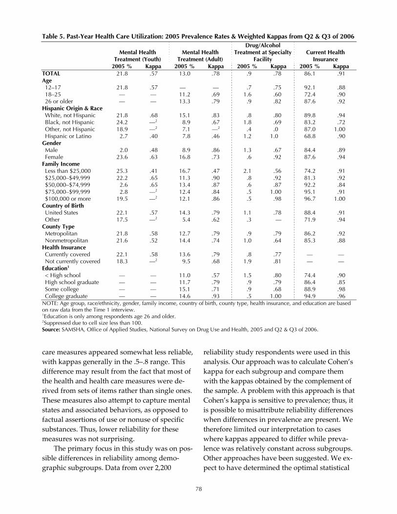
78

care measures appeared somewhat less reliable, with kappas generally in the .5–.8 range. This difference may result from the fact that most of the health and health care measures were de‐rived from sets of items rather than single ones. These measures also attempt to capture mental states and associated behaviors, as opposed to factual assertions of use or nonuse of specific substances. Thus, lower reliability for these measures was not surprising. 

The primary focus in this study was on pos‐sible differences in reliability among demo‐graphic subgroups. Data from over 2,200 

reliability study respondents were used in this analysis. Our approach was to calculate Cohen’s kappa for each subgroup and compare them with the kappas obtained by the complement of the sample. A problem with this approach is that Cohen’s kappa is sensitive to prevalence; thus, it is possible to misattribute reliability differences when differences in prevalence are present. We therefore limited our interpretation to cases where kappas appeared to differ while preva‐lence was relatively constant across subgroups. Other approaches have been suggested. We ex‐pect to have determined the optimal statistical 

Table 5. Past-Year Health Care Utilization: 2005 Prevalence Rates & Weighted Kappas from Q2 & Q3 of 2006

Mental Health

Treatment (Youth) Mental Health

Treatment (Adult)

Drug/Alcohol Treatment at Specialty

Facility Current Health

Insurance 2005 % Kappa 2005 % Kappa 2005 % Kappa 2005 % Kappa TOTAL 21.8 .57 13.0 .78 .9 .78 86.1 .91 Age 12–17 21.8 .57 — — .7 .75 92.1 .88 18–25 — — 11.2 .69 1.6 .60 72.4 .90 26 or older — — 13.3 .79 .9 .82 87.6 .92

Hispanic Origin & Race White, not Hispanic 21.8 .68 15.1 .83 .8 .80 89.8 .94 Black, not Hispanic 24.2 —2 8.9 .67 1.8 .69 83.2 .72 Other, not Hispanic 18.9 —2 7.1 —2 .4 .0 87.0 1.00 Hispanic or Latino 2.7 .40 7.8 .46 1.2 1.0 68.8 .90

Gender Male 2.0 .48 8.9 .86 1.3 .67 84.4 .89 Female 23.6 .63 16.8 .73 .6 .92 87.6 .94

Family Income Less than $25,000 25.3 .41 16.7 .47 2.1 .56 74.2 .91 $25,000–$49,999 22.2 .65 11.3 .90 .8 .92 81.3 .92 $50,000–$74,999 2.6 .65 13.4 .87 .6 .87 92.2 .84 $75,000–$99,999 2.8 —2 12.4 .84 .5 1.00 95.1 .91 $100,000 or more 19.5 —2 12.1 .86 .5 .98 96.7 1.00

Country of Birth United States 22.1 .57 14.3 .79 1.1 .78 88.4 .91 Other 17.5 —2 5.4 .62 .3 — 71.9 .94

County Type Metropolitan 21.8 .58 12.7 .79 .9 .79 86.2 .92 Nonmetropolitan 21.6 .52 14.4 .74 1.0 .64 85.3 .88

Health Insurance Currently covered 22.1 .58 13.6 .79 .8 .77 — — Not currently covered 18.3 —2 9.5 .68 1.9 .81 — —

Education1 < High school — — 11.0 .57 1.5 .80 74.4 .90 High school graduate — — 11.7 .79 .9 .79 86.4 .85 Some college — — 15.1 .71 .9 .68 88.9 .98 College graduate — — 14.6 .93 .5 1.00 94.9 .96

NOTE: Age group, race/ethnicity, gender, family income, country of birth, county type, health insurance, and education are based on raw data from the Time 1 interview. 1Education is only among respondents age 26 and older. 2Suppressed due to cell size less than 100. Source: SAMSHA, Office of Applied Studies, National Survey on Drug Use and Health, 2005 and Q2 & Q3 of 2006.

79

methodology by the time the full data set is available for analysis. Whatever the method, the important thing to determine is whether any meaningful patterns emerged in the findings and, if so, how they might translate into usable knowledge. 

One pattern that seemed reasonably appar‐ent was in the relation between age and re‐sponse consistency. Not surprisingly, youths appeared less consistent (note the lower kappas for youths than those obtained for the comple‐ment) than young adults and older adults in their reporting of substance use, particularly in the cases of lifetime and past‐year nonmedical prescription drug use and past‐year alcohol use. Young adults and older adults had fewer kappas below those of the complement of the sample, and in a few cases, appeared more con‐sistent than the other groups. However, as noted earlier, prevalence varies quite a bit by age, so the use of kappa to examine differences is somewhat limited.  

Other patterns that appeared were related to race/ethnicity. White respondents appeared to be more consistent than others in reporting past‐year substance use. If confirmed when more rigorous methods are applied, this find‐ing should trigger further analyses to determine whether the survey instrument might be cul‐turally slanted, Whites might feel less pressure to hide their substance use, or some other socio‐cultural factors might be active.  

Recent interest in Hispanics’ differential re‐sponse patterns to questionnaire items about depression and mental health also can be ad‐dressed somewhat by these data. In the cases of major depressive episode, substance depend‐ence/abuse, and serious psychological distress, the kappas attained by Hispanics appeared consistently lower than those attained by oth‐ers. Findings from the full reliability study sample may be more telling and may lead to further investigation. However, because no re‐liability study interviews were conducted in Spanish, the equivalence of the NSDUH transla‐tions cannot be examined with these data. 

A general pattern also appeared to be pre‐sent in the case of income. Greater income was generally associated with greater response con‐sistency. This result would only be surprising if educational level did not exhibit the same gen‐eral pattern of association, which it did. These findings point toward efforts to lower the read‐ing level of the instrument and to improve the comprehensibility of the supporting materials that describe the survey, the uses of the data, measures taken to enhance confidentiality, etc. In general, these findings might be seen as a re‐minder that practically all surveys are designed and conducted by persons with relatively high educational level and verbal skills, while re‐spondents come from all strata within the population of interest. Keen awareness of that notion needs to be maintained during all stages of survey design, implementation, and analysis. 

Persons attempting to analyze survey data on health disparities should be interested in the findings presented here. Consideration of the reliability of the survey instrument within the subgroups of interest is needed before conclud‐ing that the data indicate disparities. Apparent disparities may in fact be the result of failure to comprehend the instrument, words or concepts that do not translate well across groups, re‐sponse options that fail to capture the full range of possibilities, and/or a host of other potential shortcomings of the measurement process. Cul‐tural tendencies toward atypical response pat‐terns, such as underreporting, also may be responsible.  

Survey designers need to incorporate thor‐ough pretesting of measures that are intended for administration to a diverse population. Fo‐cus groups, cognitive testing, expert reviews (including experts on the subpopulations in question) and other methods have been devised as means of improving survey instrumentation, and they have been shown to produce quantifi‐able effects in reducing age‐group related vari‐ability in response (e.g., Kennet, Painter, Barker, Aldworth, & Vorburger, 2005) and other im‐provements. Budgeting of time and money for 

80

instrument development often is neglected, while interest in the measurement of health disparities increases.  REFERENCES

Cohen, J. (1960). A coefficient of agreement for nominal scales. Psychological Bulletin, 70, 213–220. 

Johnson, T. P., & Bowman, P. J. (2003). Cross‐cultural sources of measurement error in sub‐stance use surveys. Substance Use and Misuse, 38, 1447–1490. 

Johnson, T. P., & Mott, J. A. (2001). The reliability of self‐reported age on onset of tobacco, alcohol and illicit drug use. Addiction, 96, 1187–1198. 

Kennet, J., Painter, D., Barker, P., Aldworth, J., & Vorburger, M. (2005). Applying cognitive psy‐chological principles to the improvement of sur‐vey data: A case study from the National Survey on Drug Use and Health. In Proceedings of the Survey Research Methods Section of the American Statistical Association (pp. 3887–3897). Alexan‐dria, VA: American Statistical Association. 

Kessler, R. J., Barker, P. R., Colpe, L. J., Epstein, J. F., Gfroerer, J. C., Hiripi, E., et al. (2003). Screening for serious mental illness in the general popula‐tion. Archives of General Psychiatry 60, 184–189. 

Landis, J. R., & Koch, G. G. (1977). The measurement of observer agreement for categorical data. Bio‐metrics, 33, 159–174.  

SAMHSA. (2005). 2006 National Survey on Drug Use and Health: Reliability study protocol. Office of Applied Studies, Internal Report. 

SAMHSA. (2007). 2006 NSDUH methodological re‐source book. Office of Applied Studies. Retrieved May 30, 2007, from www.oas.samhsa.gov/ nsduh/methods.cfm#2k6 

Shea, S., Stein, A. D., Lantigua, R., & Basch, C. E. (1991). Reliability of the Behavioral Risk Factor Survey in a triethnic population. American Jour‐nal of Epidemiology, 133, 489–500. 

Shillington, A. M., & Clapp, J. P. (2000). Self‐report stability of adolescent substance use: Are there differences for gender, ethnicity and age? Drug and Alcohol Dependence, 60, 19–27. 

Stein, A. D., Lederman, R. I., & Shea, S. (1993). The Behavioral Risk Factor Surveillance System questionnaire: Its reliability in a statewide sam‐ple. American Journal of Public Health, 83, 1768–1772. 

Stein, A. D., Courval, J. M., Lederman, R. I., & Shea, S. (1995). Reproducibility of responses to tele‐phone interviews: Demographic predictor of discordance in risk factor status. American Jour‐nal of Epidemiology, 141, 1097–1106.

   

81

FEATURE PAPER: Disability: Collecting Self-Reports and Objective Measures from Seniors

Patricia Gallagher, University of Massachusetts Boston Kate Stewart, Harvard School of Public Health

Carol Cosenza and Rebecca Crow, University of Massachusetts Boston   INTRODUCTION

To estimate disability in the elderly popula‐tion, national longitudinal surveys of aging and health frequently include self‐reported meas‐ures of ability to conduct activities of daily liv‐ing (ADLs, such as walking around inside, bathing, dressing, and eating) and instrumental activities of daily living (IADLs, such as grocery shopping, preparing meals, light housework, and managing money). These survey data typi‐cally are interpreted to reflect the health status of the elderly population and are used to pro‐ject public spending on Medicare and Medicaid programs, including demand for home‐based and nursing home care. Analyses of self‐reported survey data have found declines in disability over the past two decades, particu‐larly in the IADLs (Cutler, 2001; Freedman, Martin, & Schoeni, 2002). While the decline in self‐reported disability is likely an indicator of improved health among elders, it is unclear whether other factors may explain some of the disability decline. We hypothesized that elderly respondents who used various technologies and lived in environments that better facilitated ADL and IADL tasks would be less likely to re‐port disability compared to respondents not us‐ing these forms of assistance, and that increased use of technologies and better environments may explain some of the observed disability de‐cline.  

We conducted a pilot study with two goals: first, to begin to understand the effect of envi‐ronmental and technological factors on survey responses1 and second, to test the data collec‐

1See Stewart, Landrum, Gallagher, and Cutler (2007) for the evaluation of whether increased availability and use of environmental and technological factors explained any of 

tion methods used in the pilot test for a planned large nationwide survey of seniors. This re‐search was supported by the National Bureau of Economic Research and the National Insti‐tutes on Aging.  

This paper describes the complexities of data collection in a pilot survey of community‐dwelling elders age 70 and older. The study in‐volved a 20‐minute in‐person Computer‐Assisted Personal Interview (CAPI) and a short physical assessment using the Short Physical Performance Battery (SPPB), a well‐established performance test developed for the Established Populations for Epidemiologic Studies of the Elderly (Berkman et al., 1993; Ferrucci et al., 2000; Guralnik et al., 1994, 1995; Melzer, Tzuo‐Yen, & Guralnik, 2003) and used in the Women’s Health Study (Ostir, Volpato, Fried, Chaves, & Guralnik, 2002), as well as in other surveys of community dwelling elders (Al Snih, Markides, Ostir, Ray, & Goodwin, 2003).    INSTRUMENTATION

The survey instrument was developed based on a review of the literature, qualitative inter‐views with members of the target population (n = 10), and cognitive interviews (n = 15). The instrument began with three disability ques‐tions from the National Long Term Care Study (NLTCS). In particular, we focused on whether a respondent had problems walking around in‐side and was able to prepare meals and shop for groceries “without help” (Manton, Corder, & Stallard, 1993). These three problem areas are focused on throughout the instrument. Follow‐up questions determined if the problems were a 

the disability decline over time. The results of those analy‐ses are beyond the scope of this paper. 

82

result of a health condition, the expected dura‐tion of the problem, and whether respondents received any help for these problems in the last three months.  

The next section asked about specific medi‐cal conditions, including arthritis, heart condi‐tion, and having broken a hip. A series of vignettes followed. Each vignette was gender‐matched to the respondent and described imaginary persons with varying levels of mo‐bility and functioning problems. Respondents were asked to decide whether the vignette de‐scribed someone who could do the given task “without help.” The next section went into more depth about walking around inside. A se‐ries of questions about grocery shopping fol‐lowed. After the grocery shopping series, questions about preparing meals attempted to ascertain how the respondent prepared their meals, including use of different kitchen aids—such as dishwasher, microwave oven, etc. The instrument ended with demographic items and included a household listing and a question about total household income in 2005. Copies of the instrument are available on request. 

 SHORT PHYSICAL PERFORMANCE BATTERY

We also obtained a performance‐based measure of physical functioning with the SPPB. A summary performance score measuring lower‐extremity function was constructed on the basis of three tests: standing balance, walking speed, and ability to rise from a chair. The standing balance test involves standing with feet in a side‐by‐side, semi‐tandem, and full‐tandem position for ten seconds each. The walking speed test measures how quickly re‐spondents are able to complete a three‐meter course while walking at their usual speed. The chair stand test requires respondents to sit in a straight‐backed chair with their arms folded and to stand up without using their arms. If re‐spondents successfully stand up, they are asked to repeat the chair stand five times as quickly as possible (Guralnick et al., 1994; Guralnik, n.d.). 

SAMPLING

The frame for this household‐level sample was the most recent city censuses available for the Massachusetts cities of Boston, Cambridge, and Somerville. A city census is conducted every year in these cities, and age of household member is on the census form. Previous experi‐ence suggests that approximately 85–90% of all people 70 or older are on the census lists, mak‐ing these lists accurate and cost‐effective for identifying this age group. The same cannot be said about these lists for other age groups. From the census lists, all unique addresses con‐taining at least one person age 70 or older were eligible for selection into the sample. The sam‐ple lists were stratified by city, and a simple random sample of addresses was selected from within each city. The sample was selected within a city proportional to the number of 70+‐year‐olds living in the city. Very early in the field period, we declared addresses within a se‐lect group of six ZIP codes ineligible. Early ex‐perience interviewing within these ZIP codes, along with experience from other recent studies CSR conducted in the same locales, indicated that most people 70 or older within these ZIP codes did not speak English. The cost of at‐tempting interviews within these ZIP codes was prohibitively high, while the expected yield of completed interviews was extremely low.  

DATA COLLECTION PROCEDURES INTERVIEWER TRAINING

The interviewers for this study attended a 1.5‐day training session. All 12 professional field interviewers were women over age 40. The briefing began with a study overview and a question‐by‐question review of the instrument. The review also included an explanation of the use of “showcards” and how to handle nonstan‐dard responses. Interviewers then were trained to conduct the SPPB using a video program and “warm practice,” where the interviewers teamed up and practiced conducting the exercises on 

83

one another.  The second day of training was devoted to additional practice on the laptops and learning data transmission procedures. In‐terviewers were tested on their proficiency at all required tasks. 

 PROJECT MATERIALS

Table 1 on the following page presents a listing of all of the field materials employed in this study.  PROCEDURES

The sample file was broken into smaller subsamples of about 150 households each. In‐terviewers were assigned specific geographic areas to cover within these subsamples. Be‐cause the sample was address based, interview‐ers were allowed to interview any eligible person in the household. Just two households had more than two eligible individuals willing to participate.  

It was the responsibility of the interviewer to mail the introductory letter prior to going to a listed address. By allowing the interviewer to orchestrate this mailing rather than having it performed centrally at CSR, the interviewer had more control of sample management. This also ensured that the letter arrived close to the time the interviewer went to the household, rather than weeks ahead of time. The letters informed individuals who did not wish to participate in the study to call CSR to refuse an interview. In‐terviewers assigned the cases that refused were notified not to attempt interviews at those ad‐dresses. The prenotification letters also pro‐vided information for interested individuals to call CSR if they wished to make an appoint‐ment for an interview. These respondents pro‐vided their phone numbers, and we passed this information on to the appropriate interviewers.  

No phone calls were made before going to the households unless the respondent had called CSR. Each contact with a potential re‐spondent represents an opportunity for a re‐fusal; the best chance to elicit cooperation for an 

interview occurs when the interviewer presents the study at the doorstep.  

After letters were mailed, the interviewers went to the addresses listed on their assign‐ment sheets. Potential respondents were offered a $20 cash incentive. All respondents who par‐ticipated in an interview received the incentive; it was not necessary to undergo the physical as‐sessment to receive the money.  

HOUSEHOLD OBSERVATION FORM

After all the interviews in a household were finished, a household observation form was completed by the interviewer. This form con‐tained questions about the respondent’s cogni‐tive ability—i.e., the perceived ability to understand the interview questions—and ques‐tions about certain physical characteristics of the interior and exterior of the dwelling.  

QUALITY CONTROL/FIELD MANAGEMENT

Field interviewers audio taped their second and fifth interviews. The field manager then re‐viewed the tapes and worked with interviewers as needed to maintain quality control. Respon‐dents were asked for their phone numbers to allow for a random sample from each inter‐viewer to be called to verify that the interview was completed. 

Each interviewer was required to have a weekly conversation with the field manager to discuss their cases. This call gave interviewers the opportunity to discuss the progress of the study, their personal progress, and any particu‐lar questions or problems that they had encoun‐tered. For example, they addressed first refusals, contact problems, address and/or lan‐guage problems, and any issues that arose as a result of routine verification procedures. The manager and interviewer also identified the ar‐eas to be covered and whether additional sam‐ple was needed. 

84

Table 1. Project Materials

Assignment Disposition Sheet

Included all cases assigned to the interviewer. Included each case’s ID #, name, & address. Used to track each case’s results & when talking to the Field Manager each week.

Cover Sheet Each case had its own paper cover sheet. Used to record the each visit’s outcome, to record a final result code, & as receipt for CSR to indicate that the respondent had received the incentive. Inside each was a simplified version of the SPPB scoring section.

Letters Printed on Harvard letterhead & mailed in Harvard envelopes by the interviewer before visiting the household. Explained the study purpose, who the sponsors were, & how to contact CSR with questions/ concerns. Each interviewer also had a supply of unaddressed/not personalized letters for respondents who had not received one.

Communication Tips for Elderly People Document

Contained tips on how to communicate with elderly people, including those who are hearing &/or visually impaired & those with cognitive difficulties.

Police Information Packet

Before the study began, letters were mailed to police stations throughout Boston, Cambridge, & Somerville explaining the study & advising that interviewers would be going to households in their area. Interviewers were given a list of all the police stations, with phone numbers, for the stations that had been contacted.

Fact Sheet Contained basic study information (e.g., funder, what was involved in participating, how respondents were selected).

Show Cards (2) Laminated, printed front & back, with instrument’s closed-ended answer categories. Shown at specified questions to aid respondent recall of answer choices.

Informed Consent Form

Signed forms were required for respondents to participate in the SPPB. Explained physical tests’ purpose, sponsor, researchers, what was involved, & risks. Printed in large font & signed by both participant & interviewer.

Interviewer Observation Sheet

Included items about respondent & descriptions of certain characteristics of the residence’s interior & exterior.

Laptop Instrument was programmed using CASES (Univ. of California Berkeley). When an interview was completed, the interviewer transmitted the data to CSR via the software program PcAnywhere.

Envelopes Interviewers received 3 types: large business-reply envelopes to return cover sheets & scoring sheets; business-size envelopes to send in time & expense summaries; and small plain envelopes in which to place the respondent incentive (if the interviewer chose to use them).

Interviewer Identification

Laminated ID cards that included name, picture, the names of Harvard University & CSR, & study name.

Calling Cards Cards with CSR contact information & space for writing a note to be left if no one answered at the sampled address.

Elder Abuse Cards Cards with phone # of the MA Executive Office of Elder Affairs to be given to respondents who specifically asked for help. (None were distributed during the course of the study.)

Respondent Pay Form

Used to track distribution of cash incentives. Interviewer recorded interview date & ID # of paid respondent. Turned in to CSR on a weekly basis.

Call-In Report Used to gather weekly information re-quired by the field manager, including current status of interviewer’s sample & amount of time spent on various tasks.

Time & Expense Summary Form

Used to record mileage, time, & expenses incurred (e.g., tolls). Mailed in weekly to CSR.

Audio Tape Recorder & Cassettes

Used to tape interviews for quality control review. With respondent’s written permission, interviewers taped 2nd & 5th interviews, & throughout the field period, interviewers were instructed to record sporadic interviews for review.

Street Atlas Interviewers were provided with books of maps for the areas they were assigned.

Materials for the SPBB

Instruction sheet. Printed on card stock. Included script for the tests & diagrams outlining the 3 tests.

Chain. Used to measure walking course for gait speed test. Was slightly longer than 3 meters & had required length delineated by metal loops near each end. Was laid on the floor in a straight line to determine correct distance to mark off.

2”-wide painter’s tape. Placed on floor to delineate walking course’s start & finish, allowing participant to clearly see the beginning & end of course.

Digital stopwatch. Used to time all exercises. Some interviewers found it difficult to control; some had trouble clearing the screen. Future studies might invest in old-fashioned stopwatches with one start & stop button.

  

85

DATA COLLECTION RESULTS

A total of 441 interviews were completed between January and April 2006 for an overall response rate of 52%. The most common rea‐son for ineligibility was inability to speak Eng‐lish well enough to complete the interview. The languages most frequently encountered were Chinese, Spanish, and Russian. Reasons that eligible respondents were not interviewed included refusals (26%), cognitive problems identified either prior to the interview or by the respondent’s inability to answer any three con‐secutive questions during the interview (2.3%), and an eligible respondent lived at the resi‐dence but was away for the duration of the study (1.8%). Also, there were 0.2% partial in‐terviews that could not to be completed during the field period, and for 0.6%, there were other reasons for non‐interviews. Table 2 presents the results of the data collection process at the household and person levels. 

Approximately 84% of all respondents at‐tempted the SPPB. Scores for the SPPB tests ran the full range of possible scores, from zero to twelve points. The most common reason for not attempting any of the tests was that the re‐spondent could not hold the initial position unassisted.  DISCUSSION

The success of our data collection proce‐dures may not be generalizable beyond the metropolitan Boston area—particularly to non‐urban settings. We were fortunate that there were no major winter storms during the field period. Any blizzards might have driven down response rates, driven up data collection costs, and/or extended the field period. The quality of the field staff also played a major role in the success of this project. Our seasoned staff of professional interviewers had the experience necessary to elicit cooperation from the target population. The interviewers were all also “women of a certain age” who were presuma‐bly seen as nonthreatening by prospective re‐

spondents when they appeared at the door. This study was conducted in part as a pilot test for a nationwide survey of seniors. Despite early reservations about the feasibility of sen‐iors’ willingness to have interviewers come into their homes to conduct both a face‐to‐face in‐terview and physical assessment tests, this study demonstrates that effective procedures for household interviews with urban elders can be implemented to make this an achievable goal.   REFERENCES

Al Snih, S., Markides, K. S., Ostir, G. V., Ray, L., & Goodwin, J. S. (2003). Predictors of recovery in activities of daily living among disabled older Mexican Americans. Aging Clinical and Experi‐mental Research, 15, 315–320. 

Table 2. Results Household Level A. Total Number of Households in Sample 1,107 B. Ineligible Households: TOTAL 148 Sample address not a dwelling unit 9 Sample address is group quarters 69 Sample address is vacant unit 44 Sample address in dropped ZIP code 29 C. Household Screened, No One Age 70+ Found 131 D. Household Screened, Someone Age 70+ Found 743 E. Household Not Screened, so Unknown if

Someone Age 70+ in Household 85

1. Rate at which screened household had someone age 70+: D/(C+D)=743/(743+131)=85.0%

2. Estimated number of households with someone age 70+ in unscreened households: E*0.85=85*.085=72

Person Level F. Total Number of People Age 70+ Found 930 G. People Ineligible Due to Language 154 H. People Ineligible Due to Hearing Problem 3 I. People Eligible for Interview 773 J. Eligible People Who Completed Interview 441 K. Eligible People Who Did Not Complete Inter-

view 332

1. Average number of people age 70+ in screened house-holds: F/D=930/743=1.25

2. Eligibility rate of people age 70+ in screened house-holds: I/F=773/930=83.1%

3. Rate at successfully interviewing screened eligible people age 70+: J/I=441/773=57.1%

4. Overall survey response rate: J/((I+(72*1.25*0.831))=441/(773+75)=0.520 or 52.0%

86

Berkman, L. F., Seeman, T. E., Albert, M., Blazer, D., Kahn, R., Mohs, R., et al. (1993). High, usual, and impaired functioning in community‐dwelling older men and women: Findings from the MacArthur Foundation Research Network on Successful Aging. Journal of Clinical Epidemi‐ology, 46, 1129–1140. 

Cutler, D. M. (2001). Declining disability among the elderly. Health Affairs, 20, 11–27. 

Ferrucci, L., Penninx, B. W., Leveille, S. G., Corti, M. C., Pahor, M., Wallace, R., et al. (2000). Charac‐teristics of nondisabled older persons who per‐form poorly on objective tests of lower extremity function. Journal of the American Geriatric Society, 48, 1102–1110. 

Freedman, V. A., Martin, L. G., & Schoeni, R. F. (2002). Recent trends in disability and function‐ing among older adults in the United States: A systematic review. Journal of the American Medi‐cal Association, 288, 3137–3146. 

Guralnik, J. M. (n.d.). Assessing physical performance in the older patient [CD‐ROM]. National Institute on Aging. Accessed May 22, 2007, at www.grc.nia.nih.gov/branches/ledb/sppb/ 

Guralnik, J. M., Simonsick, E. M., Ferrucci, L., Glynn, R. J., Berkman, L. F., Blazer, D. G., et al. (1994). A short physical performance battery as‐sessing lower extremity function: Association 

with self‐reported disability and prediction of mortality and nursing home admission. Journal of Gerontology, 49, M85–M94. 

Guralnik, J. M., Ferrucci, L., Simonsick, E. M., Salive, M. E., & Wallace, R. B. (1995). Lower‐extremity function in persons over the age of 70 years as a predictor of subsequent disability. New England Journal of Medicine, 332, 556–561. 

Manton, K. G., Corder, L. S., & Stallard, E. (1993). Estimates of change in chronic disability and in‐stitutional incidence and prevalence rates in the U.S. elderly population from the 1982, 1984, and 1989 National Long Term Care Survey. Journal of Gerontology, 48, S153–S166.  

Melzer, D., Tzuo‐Yun, L., & Guralnik, J. M. (2003). The predictive validity for mortality of the index of mobility‐related limitation: Results from the EPESE study. Aging, 32, 619–625. 

Ostir, G., Volpato, S., Fried, L., Chaves, P., & Guralnik, J. (2002). Reliability and sensitivity to change assessed for a summary measure of lower body function: Results from the Women’s Health and Aging Study. Journal of Clinical Epidemiology, 55, 916–921. 

Stewart, K. A., Landrum, M. B., Gallagher, P., & Cutler, D. M. (2007). Understanding self‐reported disability in the elderly population. Manuscript submitted for publication. 

 

87

FEATURE PAPER: The Validity of Self-Reported Tobacco and Marijuana Use, by Race/Ethnicity, Gender, and Age Arthur Hughes, Substance Abuse and Mental Health Services Administration

David Heller and Mary Ellen Marsden, RTI International   

INTRODUCTION

Accurate information on the incidence and prevalence of alcohol, tobacco, and illicit drug use is critical to the development of meaningful and effective prevention and treatment pro‐grams. Because minorities continue to have some of the highest rates of various diseases, reducing or eliminating health disparities re‐mains a priority in the federal government.    African Americans and Hispanics have dispro‐portionately higher rates of HIV/AIDS cases than Whites, and African Americans have lower survival rates for lung cancer than Whites (Office of Minority Health, 2005). With regard to drug use, Fendrich and Johnson (2005) showed that African Americans may provide less valid information on self‐reported drug use than other racial/ethnic groups. Re‐searchers and policymakers have long been concerned about the validity of self‐reported drug use and have provided recommendations for improvement, including the use of biologi‐cal specimens to validate self‐reports (U.S. Gen‐eral Accounting Office, 1993). A National Institutes of Health strategic plan for reducing health disparities in drug abuse and addiction recommended improving the validity of self‐reported drug use because minority popula‐tions may be differentially affected (National Institute on Drug Abuse [NIDA], 2004). The goal of this study is to examine the nature and extent of bias and discordance in self‐reported estimates of tobacco and marijuana use by race/ethnicity, gender, and age compared with results from urinalysis tests in a nationally rep‐resentative household survey.  

BACKGROUND

Findings presented in this paper are based on a study of the validity of self‐reported drug use data. This independent methodological study was modeled after the 2000 and 2001 Na‐tional Household Survey on Drug Abuse (NHSDA), a multistage probability sample of the civilian noninstitutionalized population age 12 years old or older in the 50 states and the District of Columbia. Since 2002, the survey has been called the National Survey on Drug Use and Health (NSDUH; Office of Applied Studies, 2006). The Validity Study was devel‐oped by researchers at the University of Dela‐ware, and the data collection was conducted by RTI International.1 Funding was provided by NIDA and the Substance Abuse and Mental Health Services Administration (SAMHSA). More complete findings from this study are available in Harrison, Martin, Enev, and Har‐rington (2007). The Validity Study used the NHSDA questionnaire and data collection methods, except that the Validity Study was conducted in the coterminous U.S. only, inter‐views were not conducted in Spanish, the sample was limited to persons age 12–25 in a sample separate from the main NHSDA, a maximum of one person per household was interviewed, and hair and urine specimens were collected. The NHSDA questionnaire was adapted to obtain information on time periods associated with the windows of drug detection in hair and urine. Because of problems encoun‐tered with the collection and analysis of hair specimens during the study (insufficient quan‐tity for testing and few positive results), analy‐ses comparing self‐reports with the results of 

1 RTI International is a trade name of Research Triangle Institute. 

88

hair testing are not presented in Harrison et al. (2007) or in this paper. 

The total number of respondents in the Va‐lidity Study was 4,465 over the two‐year data collection period (2000 and 2001), with a 74.3% weighted interview response rate. Of those completing the interview, 89.4% provided hair, urine, or both; of these, 80.5% provided both, 4.7% provided only urine, and 4.3% provided only hair. Additional interview and urine speci‐men response rates by race/ethnicity, gender, and age are presented in Table 1. Respondents received $25 each to provide a hair and a urine specimen, for a total of $50. Urine drug testing was conducted for cotinine (tobacco), mari‐juana, cocaine, opiates, and amphetamines.  METHODS

For this report, a positive test for tobacco use was recorded if a respondent was found to have a concentration of 100 nanograms per mil‐liliter (ng/mL) or more of cotinine, the principal metabolite of nicotine. Testing was done using an immunoassay test (i.e., enzyme‐linked im‐

munosorbent assay, ELISA). Tobacco testing re‐sults were compared with a respondent’s self‐reported tobacco use in the past three days. These data were captured in their answers to follow‐up questions after their admission of past‐month use of cigarettes, cigars, pipes, or smokeless tobacco. Respondents who reported no past‐month tobacco use in previous questions were considered nonusers in the past three days. For marijuana, respondents whose urine speci‐mens were screened to have a concentration of 30 ng/mL of marijuana (cannabinoids) or more and confirmed to have a concentration of 2 ng/mL or more of delta‐9‐tetrahydrocannabinol carboxylic acid (THCA) were recorded as test‐ing positive. Either fluorescence polarization immunoassay (FPIA) or enzyme‐multiplied immunoassay technique (EMIT) was used for screening, depending on when the sample was tested, and confirmation tests were done through gas chromatography/mass spectrome‐try (GC/MS) testing. Self‐reported three‐day use of marijuana was recorded in response to a similar follow‐up question as that for tobacco; however, respondents also were asked about 

Table 1. Response Rates & Sample Sizes for the Validity Study, by Demographic Characteristics

COMPLETED INTERVIEW PROVIDED URINE SAMPLE

CHARACTERISTIC Selected Persons1

# Respondents

Weighted Response Rate2

# Respondents

Weighted Response Rate

TOTAL 5,985 4,465 74.3% 3,810 85.1% Race/Ethnicity White, non-Hispanic 3,848 2,866 74.8 2,447 85.1 Black, non-Hispanic 809 603 77.0 528 86.5 Other, non-Hispanic 352 323 73.5 260 85.4 Hispanic 954 673 70.3 575 84.0

Gender Male 2,898 2,161 74.5 1,873 86.6 Female 3,063 2,304 74.4 1,937 83.6

Age 12–17 2,940 2,303 77.9 1,977 85.9

12–14 1,456 1,173 80.4 1,006 85.9 15–17 1,481 1,130 75.5 971 85.9

18–25 3,045 2,162 71.3 1,833 84.5 18–20 1,185 890 74.9 764 85.3 21–25 1,851 1,272 69.2 1,069 83.9

1 Selected persons may have unknown screening information for race/ethnicity, gender, and the finer age categories (12–14, 15–17, 18–20, 21–25). Those cases have been excluded from the reported sample sizes of selected persons and the calculation of the weighted response rates for these demographic categories.

2 Weighted response rates are computed using the number of respondents based on the screening by race/ethnicity, gen-der, and age, which may differ from the corresponding demographic categories for the final number of respondents re-ported in the second column of this table. 

89

their past three‐day marijuana use in a repeat question appearing later in the questionnaire. If a respondent reported past three‐day use in ei‐ther question, he or she was considered a past three‐day marijuana user. Respondents who reported no three‐day use in the follow‐up question and did not have a valid response to the repeat question on past three‐day use were excluded. Additionally, all respondents without a valid drug test were excluded from this analy‐sis. 

In addition to weighted prevalence rates of self‐reported three‐day use and positive test re‐sults, statistics comparing self‐reporting and drug testing also are presented. These include estimates of discordance, underreporting and overreporting, bias, and correlation between discordance and bias. These measures are de‐fined below and are based on variables in the 2x2 table shown in Figure 1. In Figure 1, TN, UR, OR, and TP are weighted totals, where the weights account for dwelling unit and person‐level selection probabilities, nonresponse, and adjustment to census population estimates.  

PSR = (OR+TP)/N = Prevalence estimate based on self‐reports. 

 

PU = (UR+TP)/N = Prevalence estimate based on urinalysis results. 

 

Bias(PSR) = PSR – PU   = [(OR + TP)/N] – [(UR + TP)/N]   = (OR – UR)/N  

Relative Bias(PSR) = (PSR – PU)/PU  

[ ]2

2

( ) (1/ ) ( )

( ) ( )(1/ )

2 ( , )

SR UVariance P P N Var OR UR

Var OR Var URN

Cov OR UR

− = −

+⎡ ⎤= ⎢ ⎥−⎣ ⎦

 

( ) /Discordance OR UR N= +   

[ ( ) ( )]( , )( ) ( )Var OR Var URCorr bias discordance

Var OR UR Var OR UR−

=− +

 

 

Note that the bias and discordance measures are both a function of overreporting and under‐reporting. Tests of significance also were per‐formed to determine if the bias was statistically 

different from zero (H0: Bias = 0 vs. H1: Bias ≠ 0). Using a Bonferroni adjustment for multiple comparisons, the alpha level was adjusted from α = .05 to α = .05/11 = .0045 to account for the 11 domains presented in Tables 2 and 3. These 11 domains consist of the total, 4 race/ethnicity categories (non‐Hispanic White, Black, and “other,” as well as Hispanic), 2 genders (male, female), and 4 age groups (12–14, 15–17, 18–20, 21–25). A correlation measure between bias and discordance was included to examine the asso‐ciation between these two measures of interest. 

In addition to the comparative statistics pre‐sented in Tables 2 and 3, two logistic regression models predicting past three‐day discordance of tobacco and marijuana were constructed. Mod‐els were fit with a permanent set of nine covari‐ates, including gender, age, race/ethnicity, passive exposure in the past six months to to‐bacco or marijuana, and socioeconomic status (SES). SES was defined based on the 1990 Cen‐sus long‐form data. The four standard catego‐ries (metropolitan statistical area [MSA]/low SES, MSA/high SES, non‐MSA/low SES, and non‐MSA/high SES), based on block‐group‐level median rents and property values from both state and MSA data, were collapsed into two categories for this paper. MSA/low SES and non‐MSA/low SES were combined to define low SES; high SES was defined in a similar fash‐ion. The other four covariates in the initial set of variables were constructed from data captured in the debriefing section of the questionnaire. These include the following:  

Figure 1. Relationship between Self-Reported Use & Urinalysis Test Results Urinalysis

Negative Positive

No

TN + UR

True negatives

(TN)

Under-reporters

(UR) Self-Reported

Use

Yes Over-

reporters (OR)

True positives

(TP) OR + TP

TN + OR UR + TP TOTAL (N)

90

• Appeal (respondent did or did not receive appeal to answer questions completely and honestly),  

• Truthfulness (respondent did or did not re‐port answering questions related to sub‐stance use completely truthfully),  

• Difficulty in answering questions related to sub‐stance use (a continuous measure con‐structed from four related debriefing questions), and 

• Privacy of the interview (a continuous meas‐ure based on the interviewer’s ranking of the level of privacy during the interview). 

Additional measures of interest were consid‐ered in the modeling but were kept in the final 

models only if they were significant at α = .05. These additional measures included the geo‐graphic characteristics of census region and population density, friends’ use of cigarettes or marijuana, respondent’s self‐reported history of arrests for breaking the law, a composite meas‐ure of respondent’s frequency of demonstrating risky/dangerous behavior, and a continuous measure of respondent’s religiosity. “Religios‐ity” was composed of questions about the number of religious services attended in the past year, the importance of religious beliefs, how much religious beliefs influence decisions, and the importance of friends sharing religious beliefs. For this continuous measure, 1 indicates 

Table 2. Comparison Statistics & Prevalence Rates Based on Urinalysis Results & Self-Reported Past 3-Day Tobacco Use

DOMAIN # R

espo

nden

ts

% D

isco

rdan

ce 1

(SE)

% O

verr

epor

ters

2 (S

E)

% U

nder

repo

rter

s 3

(SE)

% S

elf-

Rep

ort

Prev

alen

ce R

ate4 (

SE)

% P

osit

ive

Uri

ne

Prev

alen

ce R

ate5 (

SE)

% R

elat

ive

Bia

s6

Cor

rela

tion

bet

wee

n B

ias

& D

isco

rdan

ce7

TOTAL 3,759 11.3 (0.6) 3.6 (0.4) 7.7 (0.5) 25.4 (1.0) 29.5b (1.1) –13.7 –0.307 Race/Ethnicity

White, non-Hispanic 2,417 10.9 (0.7) 4.0 (0.6) 6.8 (0.6) 29.3 (1.3) 32.1a (1.4) –8.6 –0.025 Black, non-Hispanic 522 14.6 (1.7) 2.1 (0.8) 12.5 (1.7) 18.4 (2.1) 28.8b (2.3) –36.2 –0.656 Other, non-Hispanic 257 7.8 (2.1) 2.1 (1.1) 5.8 (1.7) 21.6 (3.1) 25.3 (3.3) –14.6 –0.439 Hispanic 563 11.7 (1.6) 4.0 (0.8) 7.7 (1.5) 16.5 (1.9) 20.3 (2.0) –18.4 –0.535

Gender Male 1,844 11.2 (0.9) 3.4 (0.5) 7.7 (0.7) 27.3 (1.3) 31.7b (1.3) –13.6 –0.332 Female 1,915 11.4 (0.8) 3.8 (0.6) 7.6 (0.7) 23.5 (1.3) 27.2b (1.4) –13.8 –0.143

Age 12–14 994 8.7 (1.1) 1.0 (0.5) 7.7 (1.0) 2.8 (0.7) 9.4b (1.1) –70.4 –0.668 15–17 958 12.7 (1.3) 2.8 (0.6) 9.9 (1.2) 17.8 (1.6) 24.9b (1.9) –28.4 –0.600 18–20 753 11.9 (1.4) 5.9 (1.0) 6.0 (0.9) 38.2 (2.3) 38.3 (2.2) –0.2 0.092 21–25 1,054 11.7 (1.3) 4.3 (0.8) 7.4 (0.9) 37.0 (1.9) 40.1 (1.9) –7.6 –0.087

SE = standard error. a Difference between bias (self-report prevalence rate – positive urine prevalence rate) and zero is statistically significant at

the .05 level. (Bonferroni adjustment was applied for multiple testing.) b Difference between bias (self-report prevalence rate – positive urine prevalence rate) and zero is statistically significant at

the .01 level. (Bonferroni adjustment was applied for multiple testing.) 1 Discordance (%) = percentage reporting no use and testing positive or reporting use and testing negative. 2 Overreporters (%) = percentage reporting tobacco use in the past 3 days but tested negative for tobacco use. 3 Underreporters (%) = percentage reporting no tobacco use in the past 3 days but tested positive for tobacco use. 4 Self-report prevalence rate (%) = percentage reporting tobacco use in the past 3 days in follow-up questions from the

Validity Study questionnaire. 5 Positive urine prevalence rate (%) = percentage testing positive for tobacco in urinalysis. A cutoff concentration of 100

ng/mL was used to identify a specimen as positive for cotinine. 6 Relative bias (%) = [(self-report rate – positive urine rate)/(positive urine rate)] x 100%. 7 Pearson’s correlation coefficient showing the correlation between the bias (self-report prevalence rate – positive urine

prevalence rate) and discordance (disagreement between self-reported prevalence and urinalysis results).

91

“not religious” and 15 “very religious.” Re‐spondents with unknown information for any of the covariate measures were excluded from the final models. Logistic regression model re‐sults are presented in Table 4. 

 RESULTS COLLECTION OF URINE SAMPLES

Overall, 85.1% of those age 12–25 provided a urine sample during the interview (Table 1). Urine acquisition rates decreased slightly with increasing age, with 85.9% of 12–14 and 15–17 year‐olds, 85.3% of 18–20 year‐olds, and 83.9% of 21–25 year‐olds providing urine samples. A 

higher percentage of males provided urine samples than females (86.6% vs. 83.6%). An es‐timated 86.5% of Blacks, 85.1% of Whites, and 84.0% of Hispanics provided a urine sample.  TOBACCO USE

Estimates of discordance associated with self‐reported tobacco use in the past three days and urinalysis results are presented in Table 2. Among racial/ethnic groups, discordance was highest among Blacks (14.6%) compared to Whites (10.9%) and Hispanics (11.7%). Males and females exhibited a similar level of discor‐dance (both about 11%). Within age groups, youths age 12–14 exhibited the lowest amount 

Table 3. Comparison Statistics and Prevalence Rates Based on Urinalysis Results & Self-Reported Past 3-Day Marijuana Use

DOMAIN # R

espo

nden

ts

% D

isco

rdan

ce1

(SE)

% O

verr

epor

ters

2 (S

E)

% U

nder

repo

rter

s3 (S

E)

% S

elf-

Rep

ort

Prev

alen

ce R

ate4

(SE)

% P

osit

ive

Uri

ne

Prev

alen

ce R

ate5

(SE)

% R

elat

ive

Bia

s6

Cor

rela

tion

bet

wee

n B

ias

& D

isco

rdan

ce7

TOTAL 3,749 7.0 (0.4) 1.7 (0.2) 5.2 (0.4) 7.9 (0.6) 11.4b (0.6) –30.8 –0.451

Race/Ethnicity White, non-Hispanic 2,408 6.6 (0.6) 2.0 (0.3) 4.6 (0.5) 8.2 (0.8) 10.8b (0.8) –23.8 –0.413 Black, non-Hispanic 522 8.8 (1.3) 0.5 (0.3) 8.3 (1.3) 8.1 (1.6) 15.9b (1.9) –49.2 –0.879 Other, non-Hispanic 257 7.4 (1.9) 3.4 (1.7) 4.0 (1.2) 10.1 (2.3) 10.7 (2.2) –5.3 0.357 Hispanic 562 6.6 (1.1) 0.9 (0.4) 5.7 (1.2) 5.1 (1.0) 9.9b (1.7) –48.1 –0.801

Gender Male 1,842 7.9 (0.7) 1.6 (0.3) 6.3 (0.6) 9.8 (0.8) 14.6b (0.9) –32.8 –0.545 Female 1,907 6.0 (0.6) 1.9 (0.4) 4.0 (0.5) 5.8 (0.7) 7.9b (0.7) –26.9 –0.279

Age 12–14 993 2.1 (0.6) 0.6 (0.3) 1.5 (0.5) 1.1 (0.4) 2.0 (0.5) –43.2 –0.351 15–17 956 7.6 (0.9) 2.4 (0.5) 5.2 (0.8) 7.5 (1.0) 10.3 (1.2) –26.9 –0.416 18–20 748 9.0 (1.2) 2.4 (0.6) 6.6 (1.0) 13.7 (1.4) 17.9b (1.6) –23.5 –0.438 21–25 1,052 8.4 (0.9) 1.5 (0.4) 6.8 (0.9) 8.4 (1.1) 13.7b (1.4) –38.9 –0.642

SE = standard error. a Difference between bias (self-report prevalence rate – positive urine prevalence rate) and zero is statistically significant at the

.05 level. (Bonferroni adjustment was applied for multiple testing.) b Difference between bias (self-report prevalence rate – positive urine prevalence rate) and zero is statistically significant at the

.01 level. (Bonferroni adjustment was applied for multiple testing.) 1 Discordance (%) = Percentage reporting no use and testing positive, or reporting use and testing negative. 2 Overreporters (%) = Percentage reporting marijuana use in the past 3 days but tested negative. 3 Underreporters (%) = Percentage reporting no marijuana use in the past 3 days but tested positive. 4 Self-report prevalence rate (%) = Percentage reporting marijuana use in the past 3 days in follow-up or repeat questions from

the Validity Study questionnaire. 5 Positive urine prevalence rate (%) = Percentage testing positive for marijuana in urinalysis. A screening cutoff concentration

of 30 ng/mL for cannabinoids and a confirmatory cutoff concentration of 2 ng/mL for carboxy-THC were used to identify a specimen as positive for marijuana.

6 Relative bias (%) = [(self-report rate – positive urine rate)/(positive urine rate)] x 100%. 7 Pearson’s correlation coefficient showing the correlation between the bias (self-report prevalence rate – positive urine preva-

lence rate) and discordance (disagreement between self-reported prevalence and urinalysis results).

92

of discordance (8.7%) compared to between 11.7% and 12.7% for the older age groups. With few exceptions, discordance was driven by un‐derreporting; overall, there were twice as many underreporters (URs) of tobacco use as overre‐porters (ORs) (7.7% vs. 3.6%). The greatest variation occurred among Blacks (12.5% vs. 2.1%) and youths age 12–14 (7.7% vs. 1.0%). The lowest variation occurred among 18–20 year‐olds (6.0% vs. 5.9%). 

Blacks and the youngest age group (age 12–14) had the highest absolute relative bias com‐pared with others within their respective do‐mains (36.2% and 70.4%, respectively), while the absolute relative bias was similar among males and females. Looking further at age dif‐ferences, there was a negative relationship be‐tween absolute relative bias and self‐reported prevalence. As self‐reported prevalence in‐creased with age from 2.8% (age 12–14) to 38.2% (age 18–20), the absolute relative bias de‐creased from 70.4% to 0.2%. For those age 21–25, three‐day self‐reported use was slightly lower at 37.0% compared with those age 18–20, while the absolute relative bias was higher at 7.6%. 

The correlation between bias and discor‐dance was moderately high for Blacks, Hispan‐ics, and the two youngest age groups (between –0.535 and –0.656), near zero for Whites and the two oldest age groups, and low to moderate among other demographic groups (Table 2). 

Unadjusted odds ratios showed that 15–17 year‐olds were more likely to provide discor‐dant responses than 12–14 year‐olds, and Blacks were more likely to report discrepant responses than Whites. However, when controlling for SES and other variables, these relationships were no longer statistically significant (Table 4). 

MARIJUANA USE

Estimates of discordance associated with self‐reported marijuana use in the past three days and urinalysis results are presented in Ta‐ble 3. Among racial/ethnic groups, discordance was highest among Blacks (8.8%)—slightly higher than among those of “other” races/eth‐nicities (7.4%) and Whites and Hispanics (6.6%). Discordance was higher among males than fe‐males, and among age groups, it was highest among the older age groups (ages 18–20 and 21–25). As with analyses of tobacco use, discor‐dance was driven by underreporting; overall, there were three times as many URs of mari‐juana use as ORs (5.2% vs. 1.7%). The greatest variation between under‐ and overreporting oc‐curred among Blacks (8.3% vs. 0.5%) and His‐panics (5.7% vs. 0.9%). 

Blacks and Hispanics had higher relative bias than other racial/ethnic groups (49.2% and 48.1%, respectively, vs. 23.8% among Whites and 5.3% among other races/ethnicities). Rela‐tive bias was higher among males than females and highest among youths age 12–14 compared with other age groups. Similar to tobacco use, the prevalence of marijuana use increased with age among the three youngest age groups, while the relative bias decreased with age among the same groups. 

The correlation between bias and discor‐dance was high for Blacks and Hispanics (–0.879 and –0.801, respectively) and low to moderate among other demographic groups (Table 3). 

Unadjusted odds ratios showed that all older age groups were more likely to provide discordant three‐day marijuana use responses than those age 12–14 and that females were less likely than males and Blacks were more likely than Whites to report discrepant responses. Ad‐justed odds ratios showed that these relation‐ships for Blacks and females were no longer statistically significant. 

93

Table 4. Logistic Regression Models Predicting 3-Day Discordance of Tobacco & Marijuana Use

3-DAY TOBACCO DISCORDANCE 3-DAY MARIJUANA DISCORDANCE

Unadjusted Odds Odds Ratio 95% CI

Unadjusted Odds Odds Ratio 95% CI

Intercept N/A 0.03b (0.01–0.06) N/A 0.02b (0.01–0.05) Race/Ethnicity

White 1.00 1.00 (1.00–1.00) 1.00 1.00 (1.00–1.00) Black 1.40a 1.27 (0.90–1.79) 1.37a 1.14 (0.73–1.80) Hispanic 1.08 1.38 (0.97–1.96) 1.00 0.88 (0.55–1.41) Other 0.69 0.79 (0.45–1.41) 1.14 1.01 (0.52–1.95)

Gender Male 1.00 1.00 (1.00–1.00) 1.00 1.00 (1.00–1.00) Female 1.03 1.10 (0.86–1.41) 0.74a 0.85 (0.64–1.14)

Age 12–14 1.00 1.00 (1.00–1.00) 1.00 1.00 (1.00–1.00) 15–17 1.53a 1.29 (0.86–1.95) 3.82b 2.09a (1.10–3.95) 18–20 1.42 1.11 (0.73–1.69) 4.63b 2.29a (1.16–4.54) 21–25 1.39 1.16 (0.78–1.71) 4.27b 2.40a (1.21–4.76)

SES High SES 1.00 1.00 (1.00–1.00) 1.00 1.00 (1.00–1.00) Low SES 1.42b 1.23 (0.94–1.61) 1.31 1.21 (0.85–1.73)

Appeal With appeal 1.00 1.00 (1.00–1.00) 1.00 1.00 (1.00–1.00) Without appeal 1.27 1.35a (1.02–1.78) 1.23 1.20 (0.90–1.61)

Truthfulness Completely truthful 1.00 1.00 (1.00–1.00) 1.00 1.00 (1.00–1.00) Not/somewhat/mostly truthful 2.63b 2.01b (1.30–3.13) 2.51b 1.41 (0.85–2.31)

Past 6-Month Exposure1 Never 1.00 1.00 (1.00–1.00) 1.00 1.00 (1.00–1.00) Seldom 0.58 0.61 (0.34–1.11) 4.47b 3.19b (1.94–5.25) Frequently 1.45 1.30 (0.76–2.23) 9.16b 4.76b (2.87–7.89) Daily 1.84a 1.60 (0.93–2.76) 8.09b 3.09b (1.49–6.40)

How Many Friends Use2 None 1.00 1.00 (1.00–1.00) 1.00 1.00 (1.00–1.00) A few 2.16b 1.78b (1.25–2.53) 2.22b 0.91 (0.58–1.43) Most 2.28b 1.35 (0.87–2.10) 7.19b 1.75a (1.10–2.78) All 3.58b 2.18a (1.04–4.57) 6.54b 1.75 (0.76–4.03)

Region Northeast 1.49 1.26 (0.74–2.14) 0.48b 0.44b (0.27–0.72) Midwest 2.04b 1.83a (1.10–3.06) 0.68 0.62a (0.39–0.99) South 1.94b 1.67a (1.05–2.65) 0.71 0.74 (0.48–1.13) West 1.00 1.00 (1.00–1.00) 1.00 1.00 (1.00–1.00)

Population Density MSA ≥ 1 million 1.00 1.00 (1.00–1.00) — — — MSA < 1 million 1.45a 1.39a (1.03–1.88) — — — Non-MSA 1.08 0.97 (0.68–1.39) — — —

Privacy Summary Measure 1.06 1.04 (0.97–1.12) 1.03 1.03 (0.94–1.14) Difficulties Summary Measure 1.08b 1.04 (0.99–1.10) 1.09b 1.08b (1.02–1.14) Religiosity Summary Measure 0.94b 0.96a (0.92–1.00) 0.88b 0.94a (0.89–0.99) Ever Arrested for Breaking the Law

Never arrested — — — 1.00 1.00 (1.00–1.00) Arrested — — — 3.07b 1.58a (1.06–2.37)

Hosmer-Lemeshow χ2 Test Hosmer-Lemeshow χ2 Test χ2 = 19.14 df = 8 p = 0.0141 χ2 = 9.50 df = 8 p = 0.3016

CI = confidence interval. MSA = metropolitan statistical area. N/A = Not applicable. SES = socioeconomic status. — Not included in final model due to nonsignificance. a Significant at the .05 level. b Significant at the .01 level. 1 Past 6-month exposure measure refers to exposure to cigarette smoke or other tobacco in the 3-day tobacco discordance model and exposure to marijuana smoke in the 3-day marijuana discordance model.

2 How many friends use measure refers to smoking cigarettes in the 3-day tobacco discordance model and marijuana use in the 3-day marijuana discordance model.

94

DISCUSSION

Without exception, all self‐reported esti‐mates of tobacco and marijuana use exhibited a downward bias, meaning that underreporting occurred more frequently than overreporting. Blacks and youths age 12–14 had the largest bias compared with others in their respective demographic groups for both tobacco and mari‐juana use. Unadjusted odds ratios showed that older persons and Blacks were more likely than the youngest age group and Whites, respec‐tively, to report discrepant responses compared with urine test outcomes; moreover, females were less likely to misreport than males. How‐ever, after controlling on SES, privacy, truthful‐ness, friends’ use, and other theoretically relevant covariates, these relationships were no longer statistically significant, indicating that researchers finding significant racial/ethnic, gender, and age differences in measurement er‐ror should be aware of covariates that may mitigate these differences and help provide other explanations. 

Because bias is defined in this analysis as the difference between ORs and URs, estimates based on self‐reports will have small bias only if these two quantities are approximately equal. Ideally, OR and UR both should be equal to zero; however, estimates with little bias could correspond to nonzero and possibly significant discordance, whenever OR and UR are large and approximately equal. One example of this is 18–20 year‐olds reporting tobacco use in the past three days. Nearly 12% provided discor‐dant responses (OR = 5.9, UR = 6.0), yet the dif‐ference between the self‐reported estimate and the percent positive urine specimens was only 0.1% (p = .94). The very low correlation between bias and discordance for tobacco use among 18–20 year‐olds also shows that these two meas‐ures can behave quite differently. There ap‐pears to be a strong relationship between self‐reported use and absolute relative bias by age. The youngest respondents (age 12–14) had the lowest use rates and highest absolute relative bias. This finding held for both tobacco and 

marijuana use and was driven by underreport‐ing. 

An important limitation of this study stems from the imprecision of the time of use indi‐cated by the urine test. Many factors can affect the length of time after use that drugs will be detectable in urine. We chose a three‐day refer‐ence period for the self‐report measure because of the near certainty that any tobacco or mari‐juana use within the past three days would be detected. However, marijuana can sometimes be detected in urine for several weeks, particu‐larly if the quantity used was large. Thus, some respondents who had last used just prior to three days ago and who self‐reported (accu‐rately) that they had not used in the past three days probably had a positive urine test and would have been counted as URs in our analy‐sis. Thus, our estimates of underreporting (and, consequently, bias and discordance) are in‐flated to some unknown degree. Alternatively, the analysis could have focused on past‐month self‐report, virtually eliminating the overcount of URs but introducing other more frequent types of misclassification (e.g., light users who last used 4–30 days ago, denied past‐month use, and had a negative urine would be coded as true negatives; if they did report use, they would be coded as ORs). 

Future studies using biological specimens to validate self‐reports should include appropriate kinds of specimens and questionnaire items so that the validity of self‐reported drug use can be investigated for longer recency periods (e.g., past month). Although the examination of past three‐day patterns of bias and discordance is useful, social desirability effects associated with reporting very recent substance use may pro‐duce a larger bias and discordance compared with those based on past‐month use. It is im‐portant to be able to accurately match the win‐dow of detection with the recency period associated with the self‐reported estimate. In‐formation on the frequency and amount of sub‐stance consumed could help determine the appropriate classification in conjunction with 

95

the urine sample data or data from any other biological specimens. Finally, in this study, it was assumed that the urine test results were measured without error. However, this will seldom be the case, so it is important to con‐sider other approaches to analyzing and pre‐senting these kinds of data.  REFERENCES

Fendrich, M., & Johnson, T. P. (2005). Race/ethnicity differences in the validity of self‐reported drug use: Results from a household survey. Journal of Urban Health: Bulletin of the New York Academy of Medicine, 82(Supplement 3), iii67–iii81. 

Harrison, L. D., Martin, S. S., Enev, T., & Harrington, D. (2007). Comparing drug testing and self‐report of drug use among youths and young adults in the gen‐eral population (DHHS Publication No. SMA 07‐4249, Methodology Series M‐7). Rockville, MD: Substance Abuse and Mental Health Services Administration, Office of Applied Studies. Re‐trieved June 21, 2007, from http://oas.samhsa.gov/validity/drugTest.pdf  

National Institute on Drug Abuse. (2004). Strategic plan on reducing health disparities: NIH health dis‐parities strategic plan, fiscal year 2004‐2008 (re‐vised July 2004). Retrieved May 25, 2007, from www.drugabuse.gov/PDF/HealthDispPlan.pdf 

Office of Applied Studies. (2006). Results from the 2005 National Survey on Drug Use and Health: Na‐tional findings (DHHS Publication No. SMA 06‐4194, NSDUH Series H‐30). Rockville, MD: Sub‐stance Abuse and Mental Health Services Ad‐ministration. Retrieved June 21, 2007, from http://oas.samhsa.gov/NSDUH/2k5NSDUH/2k5results.htm  

Office of Minority Health. (2005, November 17). HHS Fact Sheet: Eliminating minority health dis‐parities. Retrieved May 25, 2007, from www.omhrc.gov/templates/content.aspx?ID=2138&lvl=2&lvlID=92 

U.S. General Accounting Office. (1993, June 25). Drug use measurement: Strengths, limitations, and recommendations for improvement (GAO/PEMD‐93‐18). Washington, DC: Author. Retrieved June 21, 2007, from http://archive.gao.gov/t2pbat5/ 149657.pdf

 

97

SESSION 2 DISCUSSION PAPER Joseph Gfroerer, Substance Abuse and Mental Health Services Administration

  

THE NEED FOR VALID COMPARISONS

This session focuses on a topic of increasing importance to health survey researchers: the need to accurately measure health characteris‐tics consistently across subpopulations and over time.  

Eliminating health disparities has been identified by the U.S. Department of Health and Human Services (DHHS) as one of two over‐arching goals of the Healthy People 2010 initia‐tive. Specifically, the goal is to “eliminate health disparities among segments of the population, including differences that occur by gender, race or ethnicity, education or income, disability, geographic location, or sexual orientation” (DHHS, 2000, p. 11). In addition, the U.S. Sur‐geon General has cited the elimination of health disparities among minorities as a public health priority. As a result, there has been an increase in the volume of research on health disparities and a demand for continuously collected, com‐parable data on various health characteristics among population subgroups. Population groups of most concern are those perceived as vulnerable to health problems or with reduced access to health care because of discrimination, cultural differences, or poverty (Kilbourne, Switzer, Hyman, Crowley‐Matoka, & Fine, 2006; Stewart & Napoles‐Springer, 2003). Thus, much of the research on health disparities has involved looking at data by race, ethnicity, na‐tivity, acculturation, income, and education, along with age, gender, and geographic area.  

To meet these data needs, surveys need to be designed to provide health measures that are consistent across the different categories of many key variables. Although there has been an em‐phasis on vulnerable populations, such as racial and ethnic minorities, immigrants, rural popu‐lations, and those in poverty, accurate meas‐urement by basic demographic variables, such as age, gender, region, and state is important too.  

Age differences in measurement should be of primary concern, as health problems and survey design issues vary greatly across the age spectrum. There continues to be a need for health data on children, and an area of increas‐ing concern is collecting health data on the growing population of older Americans.  

Consistent measurement across geographic areas such as region, state, substate, and ur‐banicity is critical as well. Resource allocation is often based on data for regions, states, and sub‐state areas. State and substate data also are used to assess the impact of new policies and programs. Furthermore, global health issues re‐quire comparable data across nations to assess needs and to evaluate the impact of interna‐tional health initiatives.  

Although this session has a focus on the cognitive aspects of questionnaires and the reli‐ability and validity of measurement at the re‐spondent level, the problem of assessing and attaining comparability across subgroups is much broader, involving sampling and cover‐age issues as well. Household surveys have been hampered by undercoverage of young adults, particularly young Black males, and by low response rates among the elderly. Tele‐phone surveys don’t cover nontelephone households and typically obtain response rates below 50%. Some ethnic groups of interest in disparities research may be undercovered due to incomplete listing in household surveys be‐cause of language barriers, cultural differences, or concerns about being identified to authori‐ties. Even when listed, selected persons may decline to participate in interviews for the same reasons. Media attention on immigration re‐form could potentially cause reduced coverage or response rates among Hispanics, especially along the Mexican border. While state‐by‐state comparisons are best made with surveys that use consistent methodologies across states, 

98

wide variations in response rates could result in biased comparisons even when data collection methods are consistent. State‐level response rates in the 2005 NSDUH ranged from 61% (New York) to 81% (Tennessee) (Wright, Sathe, & Spagnola, 2007). Also, interviewer effects are typically intertwined with PSU or state effects because individual interviewers usually cover a small geographic area, such as a metropolitan area or other confined area. Finally, there are situations where response bias may vary by state as a result of different cultural or legisla‐tive factors. For example, in states with more severe penalties for marijuana possession or stricter enforcement of laws, marijuana users may be more reluctant to report their use in a survey interview.   

COMMENTS ON THE PAPERS

The five papers presented in this session exhibit diverse approaches to assessing reliabil‐ity, validity, and comparability in the meas‐urement of health.  

Fleishman demonstrates a methodology for assessing measurement equivalence using mul‐tiple‐indicator multiple‐causes models (MIMIC). His analysis focuses on a composite variable based on ten items related to psycho‐logical distress, taken from the K6 (six items), the SF12 (two items) and the PHQ (two items) scales. This approach represents an excellent example of how useful information can be ob‐tained about the validity of an instrument without additional expensive data collection. When there are existing data available, the method can be used to help develop new sur‐vey items or scales, minimizing differential item functioning at the design phase. Recogniz‐ing that the K6 items originally were selected based on their consistency across groups, this analysis provides reassurance that the items in the K6 are not biased in the context of the MEPS.  

When using this kind of analysis to evaluate measurement equivalence, it is important to re‐member that multi‐item scales constructed us‐ing Item Response Theory methods are greater 

than the sum of their parts. Individual items may be more or less relevant for certain popula‐tions, but measurement equivalence is the goal for the overall scale, not necessarily individual items. As Fleishman’s analysis shows, the item asking whether everything is an effort does not have the same relevance for psychological dis‐tress among the elderly as it does for distress among younger respondents, but its selection as an item indicates it contributed adequately to the overall scale in the populations tested.  

 Recent findings from NSDUH point out the limitations of focusing only on the psychomet‐ric properties of mental health scales in assess‐ing comparability. Significant context effects were identified with the K6 scale. In the 2004 NSDUH, the half sample that was administered the K6 alone reported higher scores than the half sample in which a series of mental health “stem” questions immediately preceded the K6. Table 1 shows that the prevalence of serious psychological distress was 23% higher with the “K6 only” sample, and the discrepancies varied by age (47% higher for age 18–25) and race/ ethnicity (47% higher for Blacks). Thus, it’s critical to consider structural features of in‐struments that may influence score fluctuations (and possibly “equivalence”) along with psy‐chometric properties of scales.  

Vernon et al. address an important topic: the quality of self‐reports of colorectal cancer screening. 

Table 1. Percent of Adults Reporting K6 Score of 13 or Greater, 2004

CHARACTERISTIC K6 Alone

K6 Preceded by Other MH Questions

Age Total age 18+ 12.2% 9.9% 18–25 20.2 13.7 26–49 14.0 10.4 50+ 6.9 7.9

Gender Male 9.4 7.7 Female 14.8 12.0

Race/Ethnicity White 12.2 9.8 Black 11.9 8.1 Hispanic 12.2 10.8

99

DHHS has identified cancer screening and management as one of six focus areas in which racial and ethnic minorities experience serious disparities in health access and outcomes. The strength of this study is in its comprehensive design, which includes collecting data from pa‐tient records for validation, re‐interviews to measure reliability, and a random assignment to three separate modes (mail, phone, and face‐to‐face). The design will allow analyses of the relationship between reliability and validity, to determine if the respondents whose self‐report was incorrect were more likely to change their response in the second interview. Further analysis of this data set also should address dif‐ferences in reliability and validity by race and ethnicity. The high levels of overreporting FOBT and colonoscopy found in this study, ap‐parently due to a social desirability effect, point to the need for more research to validate self‐reports of colorectal cancer screening. In addi‐tion, the sample used in this study may not be generalizable due to the limited geographic area and population covered and the high re‐fusal rate.  

Kennet et al. present preliminary results from an important new study done within the National Survey on Drug Use and Health. The nationally representative sample of over 3,000 respondents re‐interviewed with the entire NSDUH instrument will provide data on the reliability of many different kinds of question‐naire items and constructs, ranging from basic demographic questions to attitudinal scales and complex modules that determine substance use disorders and mental problems. The data pre‐sented by Kennet et al. indicate very good reli‐ability for reporting of substance use behaviors, with no major differences across population groups, with the possible exception of youths, who report less reliably on several measures. Another area of concern is the results indicating poor reliability for Hispanics’ reporting of sub‐stance abuse and mental problems. This in‐cludes the data on Serious Psychological Distress, which is based on the K6 scale as‐

sessed in the Fleishman paper, although NSDUH uses a past‐year reference period, while the MEPS data analyzed by Fleishman is based on a 30‐day reference period.  

Gallagher et al. address another aspect of comparability—making comparisons over time when key characteristics of the population re‐lated to the measure of interest are changing. In this case, the problem is that with the increasing availability of assistive technologies and other aids that may reduce the impact of disabilities, it is not clear that the downward trend in self‐reported disability reflects improved health or is an artifact. By collecting more in‐depth in‐formation using vignettes and physical tests, the researchers plan to answer this question. While this may seem like an unusual problem unique to the study of disability, it actually represents an issue faced quite often in health surveys. How can the presence of a health condition be consistently measured in a population in which some persons are untreated and others are re‐ceiving treatment that reduces or eliminates the symptoms of the condition? This is an issue not only if treatment rates change over time, com‐plicating trend assessment, but also if treatment rates vary across population subgroups, affect‐ing comparisons and the study of disparities.  

Hughes et al. present data from a validity study done in conjunction with the NSDUH (Harrison, Martin, Enev, & Harrington, 2007). This study demonstrates that it is possible to get good cooperation rates for collecting urine and hair in a general population survey but also shows the difficulties in identifying an accurate, comparable criterion measure for validating self‐reports. The hair samples collected were not useful in validating self‐reports, and inter‐pretation of the urine results is difficult due to the uncertainties about the time period repre‐sented by the urine tests. Nevertheless, the data are consistent with prior studies that have found higher levels of underreporting of sub‐stance use among Blacks (Johnson & Bowman, 2003). Both NSDUH and Monitoring the Future (MTF) showed lower rates of marijuana use 

100

among Black youths and young adults com‐pared with Whites in 2000 and 2001, and the Youth Risk Behavior Surveillance System (YRBSS) showed rates for White and Black high school students that were about equal. But the urine tests from Hughes et al. show that Blacks age 12–25 had a 50% higher rate of use than Whites, as seen in Table 2.  

However, multivariate results (predicting marijuana discordance in a logistic regression model) show that Blacks were no more likely than Whites to provide discordant responses af‐ter controlling on socioeconomic status, passive exposure to marijuana smoke, being truthful in answering drug use questions, and other rele‐vant covariates. The correlation between bias in self‐reported marijuana prevalence and mari‐juana discordance was very high for Blacks (‐.879), suggesting that a model depicting the bias in self‐report prevalence would not show a statistically significant difference between Blacks and Whites based on these same covariates. 

Comparisons of NSDUH and MTF esti‐mates of marijuana use by grade show an in‐creasing ratio of NSDUH to MTF with increasing grade, suggesting that underreport‐ing in the household, relative to in‐school data collection, decreases with age among youths (Gfroerer, Wright, & Kopstein, 1997). Brener et al. (2006) found evidence of this differential bias 

as well in a study associated with the YRBSS. The validity study results are consistent with these findings, as seen in Table 3.   FUTURE CHALLENGES & RECOMMENDATIONS

Trends in the demographics and other char‐acteristics of the United States population point to the need for new approaches to designing and evaluating health surveys. Most notably, the nation is becoming more culturally diverse, and the population is becoming older. The Cen‐sus Bureau (2004) projects that between 2000 and 2020, the percent of the population that is Hispanic will grow from 12.6 to 17.8, and the percent Asian will increase from 3.8 to 5.4. The percent over age 65 will increase from 12.4 to 16.3. The aging population demands new data collection tools that can measure health indica‐tors accurately and consistently for older adults who often are institutionalized, mentally and physically impaired, difficult to contact because of gatekeepers and controlled access, and un‐willing to participate when they are contacted for surveys (Murphy, Eyerman, & Kennet, 2004).  

The greater need for surveys to provide comparable estimates is not independent of other challenges facing survey designers. De‐clining budgets for data collection and meth‐odological research will make it difficult to adequately do the methodological work neces‐sary to ensure comparability and to assess it af‐ter data are collected. The general trend in surveys of declining response rates can only have a negative impact on comparability. Given the importance of comparability, careful con‐sideration needs to be given to any proposed 

Table 2. Percentage Using Marijuana in Past Month Based on Self-Report Surveys and Validity Study, by Race/Ethnicity

Non

-His

pani

c W

hite

Non

-His

pani

c B

lack

His

pani

c

NSDUH, 12–17, 2001 8.5% 5.8% 7.5% NSDUH, 18–25, 2001 17.9 15.0 10.2 MTF, 8th Grade, 2000-01 8.4 8.1 12.6 MTF, 10th Grade, 2000-01 20.2 16.7 20.5 MTF, 12th Grade, 2000-01 22.9 17.0 22.1 YRBSS, 9th–12th Grade, 2001 24.4 21.8 24.6 Validity Study Self-Report (3-day), 12–25, 2000–01 8.2 8.1 5.1 Validity Study Urine Test, 12–25, 2000–01 10.8 15.9 9.9

Table 3. Estimates of Percentages of Students Using Marijuana in the Past Month, Spring 2001

Grade/Age Ratio of MTF to

NSDUH Prevalence

Ratio of Urine Test to NSDUH 3-Day

Self-Report 8th/12–14 2.49% 1.82% 10th/15–17 1.55 1.37 12th/18–20 1.48 1.30

101

use of the increasingly advocated multimode approaches to surveys. Design optimizations should include consideration of comparability across subgroups and over time. In some cases it may be desirable to allow more bias in overall estimates in order to reduce bias for compari‐sons. This is consistent with the basic principle that should be followed in designing any sur‐vey: the design should reflect and facilitate the particular analyses that will ultimately be ap‐plied to the data that is collected. 

One of the most important challenges sur‐vey methodologists face on this issue is com‐munication. Most of the general public recognizes that estimates generated from sur‐veys are not comparable when questions are worded differently or when definitions are not consistent. While survey researchers under‐stand that coverage differences, nonresponse bias variations, mode effects, context effects, in‐centive effects, and differential item functioning can affect comparability, these subtle factors are not recognized as problematic by many data us‐ers. The impact of these factors is not well un‐derstood by those outside the survey research field, so they often are overlooked or dismissed by policymakers, the media, and even some re‐searchers. Examples are easy to find in sub‐stance abuse epidemiology research literature. Survey researchers need to find better ways to inform data users of these important limitations of survey data. This is critical at both the design phase and in the reporting of results. 

REFERENCES

Brener, N. D., Eaton, D. K., Kann, L., Grun Baum, J. A., Gross, L. A., Kyle, T. M., et al. (2006). The as‐sociation of survey setting and mode with self‐reported health risk behaviors among high school students. Public Opinion Quarterly, 70, 354–374. 

Gfroerer, J., Wright, D., & Kopstein, A. (1997). Preva‐lence of youth substance use: The impact of methodological differences between two na‐

tional surveys. Drug and Alcohol Dependence, 47, 19–30. 

Harrison, L. D., Martin, S. S., Enev, T., & Harrington, D. (2007). Comparing drug testing and self‐report of drug use among youths and young adults in the gen‐eral population (DHHS Publication No. SMA 07‐4249, Methodology Series M‐7). Rockville, MD: Substance Abuse and Mental Health Services Administration, Office of Applied Studies. Re‐trieved July 11, 2007, from www.oas.samhsa.gov/validity/drugTest.cfm  

Johnson, T. P., & Bowman, P. J. (2003). Cross‐cultural sources of measurement error in sub‐stance use surveys. Substance Use & Misuse, 38, 1447–1490. 

Kilbourne, A. M., Switzer, G., Hyman, K., Crowley‐Matoka, M., & Fine, M. J. (2006). Advancing health disparities research within the health care system: A conceptual framework. American Jour‐nal of Public Health, 96, 2113–2121. 

Murphy, J., Eyerman, J., & Kennet, J. (2004). Nonre‐sponse among persons age 50 and older in the National Survey on Drug Use and Health. In S. B. Cohen & J. M. Lepkowski (Eds.), Eighth Con‐ference on Health Survey Research Methods (pp. 73–78). Hyattsville, MD: National Center for Health Statistics. 

Stewart, A. L., & Napoles‐Springer, A. M. (2003). Advancing health disparities research: Can we afford to ignore measurement issues? Medical Care, 41, 1207–1220. 

United States Census Bureau. (2004). Projected population of the United States by age and sex: 2000 to 2005. From U.S. interim projections by age, sex, race, and Hispanic origin. Retrieved March 18, 2004, from www.census.gov/ipc/www/ usinterimproj/  

U.S. Department of Health and Human Services. (2000). Healthy people 2010 (Vol. 1, 2nd ed.). Wash‐ington, DC: U.S. Government Printing Office. 

Wright, D., Sathe, N., & Spagnola, K. (2007). State estimates of substance use from the 2004–2005 National Surveys on Drug Use and Health (DDHS Publication No. SMA 07‐4235, NSDUH Series H‐31). Rockville, MD: Substance Abuse and Mental Health Services Administration, Office of Applied Studies.

 

103

SESSION 2 SUMMARY Vicki Burt, National Center for Health Statistics, and Todd Rockwood, University of Minnesota

  

This session focused on the concern that measurement error could either obscure health disparities in population subgroups or produce estimates of disparity where none exist. 

Differential item functioning (DIF) of sur‐vey items may produce observed variation in subgroup analysis not because there is a differ‐ence in the underlying condition of interest, but because the respondents in the subgroups in‐terpreted the question differently. That is, it may be measurement error. John Fleishman (AHRQ) presented an example of using the multiple‐indicator multiple‐causes (MIMIC) models to assess DIF or measurement non‐equivalence. In this example using ten items re‐lated to mental health status, no DIF was detected. Most of these measures had been sub‐ject to DIF analysis prior to inclusion in the sur‐vey, and those with DIF were excluded from the questionnaire.  

This approach can be utilized in the evalua‐tion of measures when multicultural research is done. This approach will permit analysts to po‐tentially avoid attributing measurement differ‐ences to cultural differences.  

Vernon presented a comprehensive study of the reliability and validity of four colorectal cancer screening test self‐reports (home fecal occult blood test, sigmoidoscopy, colonoscopy, and barium enema). The validity was deter‐mined by comparison to medical records. In this instance, a homogeneous population was selected. The validity estimates were evaluated for three modes of administration (mail, tele‐phone, and face‐to‐face). Additionally, test‐retest reliability of the questionnaire was as‐sessed using three time periods (two weeks, three months, and six months). This study is an exemplary example of how to evaluate ques‐tionnaire items when it is anticipated the ques‐tions will be used broadly in terms of varying modes and length of recall.  

Kennet presented results of a large reliabil‐ity study conducted for the National Survey of Drug Use and Health (NSDUH). In 2006, 3,100 NSDUH respondents were reinterviewed 5–15 days after their first interview. Items evaluated weren’t limited to drug use questions but to more general health questions (high blood pressure), some scales (K6 psychological dis‐tress scale), and health insurance and utiliza‐tion. Reliability was assessed for non‐Hispanic Blacks, non‐Hispanic Whites, and Hispanics. However, due to the low proportion of NSDUH interviews completed in Spanish, reliability was not evaluated in Spanish.  

Gallagher described a pilot test designed to monitor disability in older persons to assess if differential response is influencing observed trends. In particular, there is concern that the availability and use of new technologies and environmental and behavioral modifications decreases respondents’ propensity to report disability. This study evaluated the correlation between raw survey responses, responses ad‐justed for observable characteristics, vignette‐adjusted survey responses, and actual physical functioning to understand whether differential reporting may be occurring.  

Finally, Hughes presented a study of the va‐lidity of self‐reported drug use across race and ethnic subgroups. Four hundred NSDUH re‐spondents received remuneration for a hair and/or urine specimen, and 80% provided a sample. Respondents were asked about three‐ and seven‐day use of tobacco and marijuana (as well as other substances, findings for which were not discussed during this presentation). For both tobacco and marijuana, more underre‐porting than overreporting occurred. While it initially appeared that Blacks were more likely than Whites to report discrepant responses compared with urine test outcomes for both to‐bacco and marijuana, the relationships did not 

104

remain statistically significant after theoreti‐cally relevant covariates were added to the model.  

The discussant reviewed other sources of bias that might affect subgroup estimate com‐parability. 

These five interesting papers highlighted approaches to evaluating measurement error that may be due to differences in understand‐ing, differences in recall and potentially differ‐ences in truthfulness and stimulated a wider ranging discussion.  

Floor discussion of validity focused on two issues: (1) evaluation of the validity of a survey item across populations and (2) comparison of self‐reported data to biological or physical markers.  

Relative to the first issue, audience mem‐bers raised a number of different questions that fall into the general categories of interviewers and translation/cultural issues relative to in‐struments and administration. The discussion regarding interviewers focused on the fit be‐tween the knowledge and skills of interviewers and the substantive focus of the research (e.g., nurses used as interviewers in the assessment of functional status in the elderly). A second in‐terviewer‐related topic was the fit between the interviewers and the population (e.g., matching on gender, ethnicity), and discussion focused on the trade‐offs associated with purposive se‐lection of interviewers. For example, because of professional training, nurses might be more likely to encourage and motivate respondents to perform, which could affect measurement; at the same time, their professional credentials may or may not reduce nonresponse. The dis‐cussion around ethnicity addressed inter‐viewer‐respondent matching and took into consideration cultural and translation issues as‐sociated with survey instruments. Survey methods are primarily a form of “White mid‐dle‐class” communication, and we are not just overcoming translation issues associated with surveys but also overcoming cultural issues as‐sociated with the methodology itself. Partici‐

pants clearly acknowledged the need for further effort on translation and administration around diverse cultures; however, the costs of the work are large and accepted standards around cultural competency and survey meth‐ods have not yet been fully articulated. 

Regarding the second issue—comparison of self‐reported data to a biological or physical marker—two concerns emerged: (1) how do we procure samples, and (2) how are they used in validity analysis? Discussion on sample pro‐curement focused on the rate at which respon‐dents are willing to offer one, two, or more biological samples or refuse collection of such samples; is refusal differentially split across in‐dividuals who do indicate drug use as opposed to those who do not? The concern was that there might be a relationship between the bio‐logical markers being sought and willingness to participate in a survey. Specifically, those who are likely to test positive make up the majority of those who refuse. The issue remaining to be addressed is whether there is a systematic rela‐tionship between engaging in/abstaining from the self‐reported behavior and the samples be‐ing collected, and if so, what can be done to deal with the potential refusal differential? 

Other themes that emerged during the dis‐cussion ranged from the principles associated with using a “gold standard” methodology, to how we should deal with the constraints that data collection places on our ability to make comparisons. Discussion of the latter centered on different timeframes often associated with self‐report vs. biological markers. This included the timing of measurement, as well the ability to map self‐reports onto available biological data. For example, in the NSDUH, respondents are typically asked about substance use during the past 30 days, yet available biological mark‐ers, such as urine tests, have a much shorter de‐tection window. This issue of differences in detection windows was a repeated theme, as was and the importance of recognizing that an unknown amount of the false positives and false negatives is likely due to these differences.  

105

Additional discussion focused on the incon‐sistency between self‐report and biological markers in the case of overreporting—that is, drug use is self‐reported but no biological marker is found. It was noted that “gold stan‐dards” are fallible, and this could be the source of some of the error. It also is possible that the desire to report no drug use may not be the same across all parts of the population. There is some evidence to suggest, for example, that some adolescents overreport substance use. 

There was also discussion about the use of validity correction factors to introduce statisti‐cal adjustments for overreporting or underre‐porting. In this approach, a detailed set of information (self‐report, biological) is obtained 

from a portion of the sample and used as an ad‐justment for the remainder of the sample. It was indicated that there are strengths to such an approach, but concerns exist about the influ‐ence that correction factors can have on the overall covariate measures.  

The final validity‐related issue discussed was how validity is conceived; it was argued that the “gold standard” model is not necessar‐ily the ideal model. Instead, a model drawing on triangulation or multiple operationalism may be a more preferred model to evaluate and establish validity.

 

107

INTRODUCTION TO AND DISCUSSION OF SESSION 3: Challenges of Collecting Survey-Based

Biomarker and Genetic Data Timothy J. Beebe, Mayo Clinic College of Medicine

  INTRODUCTION 

It is becoming increasingly apparent that a fuller understanding of health and health out‐comes will require the simultaneous collection and analysis of data related to genes, the envi‐ronment, and behaviors. The household survey appears to be an ideal medium for the collection (or linking) of these various types of informa‐tion. While the household survey has long been used to collect vast amounts of data related to demographic, social, psychological, and behav‐ioral influences on health and health outcomes, the collection of the types of biological meas‐ures listed in Table 1 ushers in a host of new benefits. As Weinstein and Willis (2000) indi‐cate, the benefits of linking biological meas‐ures with survey data include (1) obtaining population‐representative data from non‐clinical samples, (2) calibrating self‐reports with other measures of health and disease, (3) explicating pathways and elaborating causal linkages between social environment and health, and (4) linking genetic markers with survey materials. The papers in this session reflect the range of topics that can be informed by this design, including aging (Smith et al.), psychiatric illness (Boyle et al.), breast cancer (Parsons et al.), general illness and injury (Johnson et al.), and adolescent health (Lad‐ner). The coupling of survey and biomeasure data is also responsible for enhancing our understanding of the determinants of and treatments for a range of diseases, including various cancers, cardiovascular disease, gas‐trointestinal disease, arthritis, and substance abuse disorders. 

There is evidence that surveys are increas‐ingly including biomarker and genetic data (hereafter referred to as “biomeasures”). Us‐

ing the key words “(survey OR questionnaire) AND (biospecimen OR biomarker OR gene OR genotype),” we conducted a PubMed search for articles that indicate the use of both biomeasure and survey data and present the results in Fig‐ure 1. It is apparent from this figure that the publications with survey‐based biomeasure data have increased in the past 20 years, both in terms of raw numbers of publications and per‐centage of total publications. For example, within just the last decade, a threefold increase in the number of publications with a reference to survey‐based biomeasure collection was ob‐served, with approximately 1,000 publications of this nature in 1996 and 3,000 in 2006, or 

Table 1. Biological Measures Related to Demographic, Social, Psychological, & Behavioral Influences & Health Outcomes SOURCE Cardiovascular System

Systolic blood pressure Exam Diastolic blood pressure Exam

Metabolic System Body mass index/waist-hip ratio Self-report/exam Total cholesterol Blood HDL/LDL cholesterol Blood Homocysteine Blood Glycosylated hemoglobin Blood

Inflammation & Coagulation Factors IL-6, CRP, low cholesterol Blood Albumin Blood Fibrinogen Blood

Antioxidant Profiles Blood

Hypothalamic Pituitary Adrenal Axis Cortisol Urine DHEAS Blood

Sympathetic Nervous System Norepinephrine Urine Epinephrine Urine

Renal Function Creatinine clearance Blood/urine

Lung Function Peak flow rate Exam

Source: Crimmins & Seeman (2000).

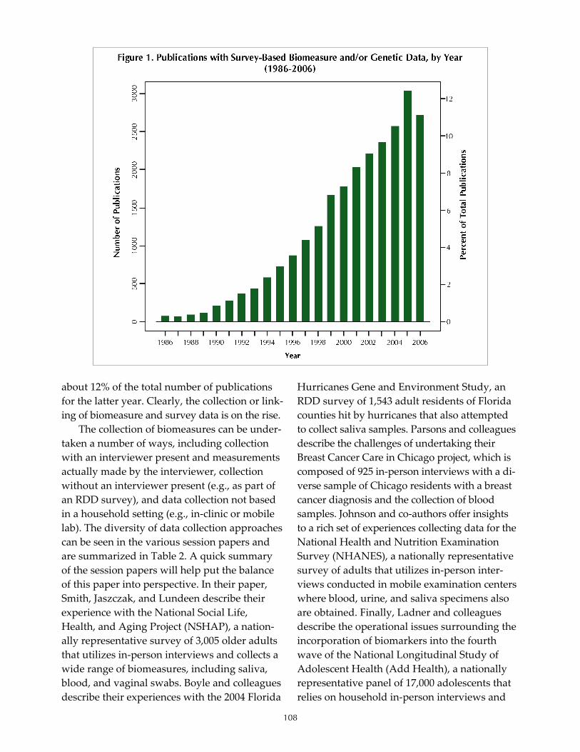
108

about 12% of the total number of publications for the latter year. Clearly, the collection or link‐ing of biomeasure and survey data is on the rise.  

The collection of biomeasures can be under‐taken a number of ways, including collection with an interviewer present and measurements actually made by the interviewer, collection without an interviewer present (e.g., as part of an RDD survey), and data collection not based in a household setting (e.g., in‐clinic or mobile lab). The diversity of data collection approaches can be seen in the various session papers and are summarized in Table 2. A quick summary of the session papers will help put the balance of this paper into perspective. In their paper, Smith, Jaszczak, and Lundeen describe their experience with the National Social Life, Health, and Aging Project (NSHAP), a nation‐ally representative survey of 3,005 older adults that utilizes in‐person interviews and collects a wide range of biomeasures, including saliva, blood, and vaginal swabs. Boyle and colleagues describe their experiences with the 2004 Florida 

Hurricanes Gene and Environment Study, an RDD survey of 1,543 adult residents of Florida counties hit by hurricanes that also attempted to collect saliva samples. Parsons and colleagues describe the challenges of undertaking their Breast Cancer Care in Chicago project, which is composed of 925 in‐person interviews with a di‐verse sample of Chicago residents with a breast cancer diagnosis and the collection of blood samples. Johnson and co‐authors offer insights to a rich set of experiences collecting data for the National Health and Nutrition Examination Survey (NHANES), a nationally representative survey of adults that utilizes in‐person inter‐views conducted in mobile examination centers where blood, urine, and saliva specimens also are obtained. Finally, Ladner and colleagues describe the operational issues surrounding the incorporation of biomarkers into the fourth wave of the National Longitudinal Study of Adolescent Health (Add Health), a nationally representative panel of 17,000 adolescents that relies on household in‐person interviews and 

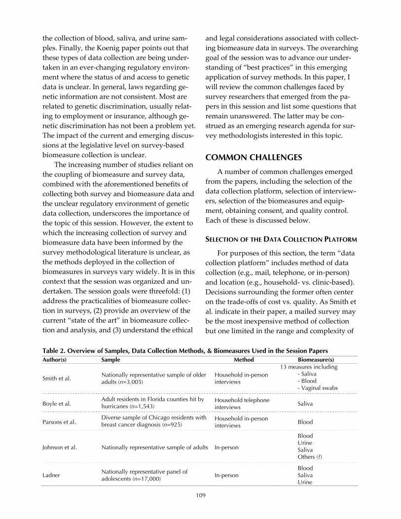
109

the collection of blood, saliva, and urine sam‐ples. Finally, the Koenig paper points out that these types of data collection are being under‐taken in an ever‐changing regulatory environ‐ment where the status of and access to genetic data is unclear. In general, laws regarding ge‐netic information are not consistent. Most are related to genetic discrimination, usually relat‐ing to employment or insurance, although ge‐netic discrimination has not been a problem yet. The impact of the current and emerging discus‐sions at the legislative level on survey‐based biomeasure collection is unclear.  

The increasing number of studies reliant on the coupling of biomeasure and survey data, combined with the aforementioned benefits of collecting both survey and biomeasure data and the unclear regulatory environment of genetic data collection, underscores the importance of the topic of this session. However, the extent to which the increasing collection of survey and biomeasure data have been informed by the survey methodological literature is unclear, as the methods deployed in the collection of biomeasures in surveys vary widely. It is in this context that the session was organized and un‐dertaken. The session goals were threefold: (1) address the practicalities of biomeasure collec‐tion in surveys, (2) provide an overview of the current “state of the art” in biomeasure collec‐tion and analysis, and (3) understand the ethical 

and legal considerations associated with collect‐ing biomeasure data in surveys. The overarching goal of the session was to advance our under‐standing of “best practices” in this emerging application of survey methods. In this paper, I will review the common challenges faced by survey researchers that emerged from the pa‐pers in this session and list some questions that remain unanswered. The latter may be con‐strued as an emerging research agenda for sur‐vey methodologists interested in this topic.   COMMON CHALLENGES

A number of common challenges emerged from the papers, including the selection of the data collection platform, selection of interview‐ers, selection of the biomeasures and equip‐ment, obtaining consent, and quality control. Each of these is discussed below.  SELECTION OF THE DATA COLLECTION PLATFORM

For purposes of this section, the term “data collection platform” includes method of data collection (e.g., mail, telephone, or in‐person) and location (e.g., household‐ vs. clinic‐based). Decisions surrounding the former often center on the trade‐offs of cost vs. quality. As Smith et al. indicate in their paper, a mailed survey may be the most inexpensive method of collection but one limited in the range and complexity of 

Table 2. Overview of Samples, Data Collection Methods, & Biomeasures Used in the Session Papers Author(s) Sample Method Biomeasure(s)

Smith et al. Nationally representative sample of older adults (n=3,005)

Household in-person interviews

13 measures including - Saliva - Blood - Vaginal swabs

Boyle et al. Adult residents in Florida counties hit by hurricanes (n=1,543)

Household telephone interviews Saliva

Parsons et al. Diverse sample of Chicago residents with breast cancer diagnosis (n=925)

Household in-person interviews Blood

Johnson et al. Nationally representative sample of adults In-person

Blood Urine Saliva Others (?)

Ladner Nationally representative panel of adolescents (n=17,000)

In-person Blood Saliva Urine

110

biomeasures that can be collected. The in‐person interview allows for the widest range of biomeasure collection, but it is also the most expensive. An in‐person interview conducted in the clinic setting may offer an even better range of biomeasure collection due to the availability of relevant biospecimen collection equipment, but some respondents may be disinclined to come into the clinic or may be otherwise ham‐pered in their ability to do so due to lack of in‐surance and transportation. 

Respondent capacity and motivation also have some bearing on what data collection plat‐form is used. As mentioned above, some re‐spondents may be disinclined to come into a clinical setting for the interview and/or biomeasure collection. Similarly, respondents may be unwilling or unable to follow the neces‐sary instructions for the collection of the rele‐vant biomeasure collection, even if it is something as relatively simple as a buccal swab. Again, there are trade‐offs in the selec‐tion of method that figure in cost, quality, re‐spondent capacity, and motivation.  SELECTION OF INTERVIEWERS

If one is to pursue the use of an in‐person interview, there appears to be a lack of consen‐sus on what type of interviewer is best suited to undertake both the survey and biomeasure col‐lection. In NHANES, Johnson et al. found that phlebotomists as interviewers increased the quality of the data and conclude that training phlebotomists to be interviewers is easier than the converse (training interviewers to draw blood). However, Smith and colleagues found it easier to train interviewers to collect the bio‐specimens than to train health care workers to be interviewers for the NSHAP. Clearly, train‐ing is a crucial component of biomeasure collec‐tion, whichever tack is taken by researchers. Interviewers also need to have buy‐in and be willing to work with the specimens, such as keeping saliva vials in their freezers. Medical malpractice insurance may be necessary for in‐terviewers who are not medically trained. Both 

Smith et al. and Ladner offer nice primers on how best to train interviewers to collect a wide range of biomeasures. 

 SELECTION OF BIOMEASURES & EQUIPMENT

In her paper on the Add Health project, Ladner does a nice job detailing the calculus un‐derlying the selection of various biomeasures. When doing face‐to‐face collection, all materials must be lightweight, easy to carry, and possible for lay interviewers to collect. As is the case with the selection of the data collection platform, de‐cision making in this realm is guided by trade‐offs between cost and data quality. Historically, blood draws have been the gold standard, as they are seen as providing the greatest yield of whatever is sought (e.g., DNA). However, the collection of blood is often the most expensive since it requires in‐person interviews for the most part and the potential use of phlebotomists, as with NHANES. But even within the realm of saliva collection, there is variability in cost and quality. King and colleagues (2002) found that buccal swabs and mouthwash offer DNA sam‐ples of comparable quality but that swabs are about half the price per sample of mouthwash rinses ($8.50 vs. $18.00, respectively) and that re‐spondents found the swab instructions easier to follow. A common approach in genetic epidemi‐ology is to ask for blood first and collect saliva if blood collection is refused (Lum & Marchand, 1998). Packaging and shipment of specimens is very important, and costly as well. Different specimens need to be shipped in different ways; a system should be in place to track shipments and follow up on delinquent shipments should be built in to the design. 

The selection of biomeasure also is dictated by the perceived level of intrusion where blood draws are presumed to be most invasive and sa‐liva the least, at least in the area of fluid bio‐specimens. In the Parsons et al. paper, and in the Smith et al. paper to a certain extent, tacit sup‐port for this notion is offered by the varied con‐sent rates they observed for the various fluid draws. For example, Parsons and colleagues 

111

found observed consent rates in the 90% range for medical record, pathology report, and tissue reviews but that consent dropped to 76% for the blood draw. In the Smith et al. paper, con‐sent rates were very high, with the exception of the vaginal swab, which was still a respectable 67%. This issue is discussed in greater depth in a later section of this paper.  OBTAINING CONSENT

The issue of obtaining consent in the context of biomeasure collection is quite complex and multifaceted and likely warrants a session of its own at some future conference. Koenig covers many of these issues in her paper, and the book Cells and Surveys: Should Biological Measures Be Included in Social Science Research? (Finch, Vaupel, & Kinsella, 2000) provides in‐depth coverage of the social and ethical issues of in‐corporating biomeasures into survey studies. The main issue here, as pointed out in the Smith et al. paper, is that most respondents are unfamiliar with the coupling of questionnaires and biomeasure collection. As such, what we know about consent in the classical survey data collection context may not be transferable to the realm of biomeasure collection. Due to the lack of regulation, how the collection is described to participants is not consistent. It can be de‐scribed as DNA or genetic material, but also as a mouthwash sample buccal cell sample or sa‐liva sample. This may, in turn, affect respon‐dents’ cooperation. Smith and colleagues found that a detailed description of the biospecimen collection in an advance letter brought about an onslaught of refusal calls. On the flip side, Par‐sons and colleagues argue for full disclosure in the consenting process. It is not clear whether IRBs will allow for less than full disclosure of all aspects of the biomeasure collection in this process, however. Furthermore, it is unclear if one’s genetic material is “identifiable.” While DNA is unique to a person, it is not clear that you can identify a person from their DNA—at least not at this time. DNA does not qualify as protected health information under HIPAA, so 

technically if other HIPAA identifiers are stripped, DNA is de‐identified data. How does one convey such risk levels to lay respondents? 

While a survey itself may have a relatively simple consent process, adding biomarker data adds new dimensions. Consent often is divided into multiple sections, where respondents can choose in which parts of the survey they want to participate. For the NHANES study described by Johnson and colleagues, certain biomarkers are grouped (e.g., environmental exposure), while some are specific (e.g., PSA test). This is the reason we see variable cooperation rates for different measures. Koenig describes a “tiered” consent process and access to biospecimens based on the number of Single Nucleotide Polymorphisms (SNPs) collected and/or made available whereby biospecimens collecting > 75 SNPs are rated high risk, < 20 SNPs intermediate risk, and no SNPs low risk. One of the goals of this approach is to provide adequate disclosure and education about the risk calculus of participation. Along these lines, future use of the data also needs to be explained—will the data be stored, and if so, for how long and what other tests will be performed? This is especially impor‐tant with genetic data, where we may not know what types of analyses we can do in the future.  

Another major issue is how and when to report the results of the biospecimen testing back to respondents. According to the Koenig paper, past practice in this area was to not re‐port back any results lacking clear implications for the participant. However, it is not clear how good some of the emerging genetic/genomic tests are or whether they are appropriate for clinical use. Also, as the number of genetic tests increases, the chance of spurious findings in‐creases. One of the major questions in this area is, are the obligations of survey researchers dif‐ferent than clinicians? Another question relates to a variant on Heisenberg’s Uncertainty Prin‐ciple, which states that one cannot observe a phenomenon without disturbing it. In this con‐text, the act of collecting biomeasures, particu‐larly information about genetic risks, may cause 

112

respondents to change their behavior if that in‐formation is filtered back to them. This would be particularly problematic in panel studies that require follow‐up data collections.  QUALITY CONTROL

Biomarker data also increases the potential for error. In addition to the usual sources of sur‐vey error, there is error associated with the col‐lection and shipment of biological specimens and laboratory error. Errors in collection and shipment can come from incorrect recording of data by the interviewer or incorrect collection of the sample by the respondent. The Add Health study has tried to prepare for this by having blood pressure data keyed by the interviewers but also downloaded directly to the computer from the blood pressure cuff. Certain specimens have temperature constraints (must be frozen, cannot get too warm), and incorrect storage may destroy specimens. Table 3 offers a sam‐pling of the different sources of error that are 

introduced with the addition of biomeasures to the survey data collection. 

The increase in error sources necessitates and underscores the importance of incorporat‐ing strict quality control mechanisms into the survey investigations. As both Johnson et al. and Ladner point out in their papers, the need for quality control increases with the number of biomeasures collected. Johnson and colleagues enumerate the possible implications of low quality control where whole batches of NHANES data were rendered unusable be‐cause of contamination. Ladner offers a nice primer on how to plan for complex survey and biomeasure data collection that can serve as a model for others.  OUTSTANDING QUESTIONS/ EMERGING RESEARCH AGENDA

A lot of the data collection practices associ‐ated with including biomeasures in surveys seem to be guided by clinical researchers and/or epidemiologists. The extent to which current practices in this area are informed by trained health survey research methodologists is not clear. One of the shortcomings in our current state of knowledge in survey‐based biomeasure collection is the absence of methodological ex‐perimentation. This is not intended to be an in‐dictment of the papers presented in this session but more a call to action on the part of health survey methodologists who have successfully embedded methodological experiments in large‐scale studies in the past. Below, I list a number of methodological questions that re‐main unanswered. The purpose of listing these is to help shape future investigations in the realm of survey‐based biomeasure data collec‐tion. The list is by no means exhaustive. For ex‐ample, much work in the area of ethics and informed consent is needed but not highlighted below. In addition, weighty analytical issues, such as the reduction of the types of high‐dimensionality data generated in genetic stud‐ies and the problem with extremely low inci‐dence/prevalence of some conditions and the 

Table 3. Error Sources in the Collection of Survey-Based Biomeasure Data Source Examples

• Failure/inability to attend study site Survey respondent • Failure to follow instructions (e.g.,

fasting) • Concerns about dispositions of

specimens

• Equipment failure or damage in transportation

Failure of the collection apparatus • Loss of electrical power • Technician absence

• Failure to follow specific protocols • Mislabeling of containers

Errors in specimen collection • Breakage, loss, or mishandling of

specimens

Mishandling in specimen transportation

• Failure to get specimen to lab in timely manner

• Loss or breakage of containers • Microbial contamination or failure

to store at correct temperature

• Loss, breakage, or contamination of specimens

Long-term specimen storage • Inadequate labeling/transcription

• Lack of appropriate procedures Laboratory determinations • Inadequate quality control Source: Wallace (2000).

113

effect of that on sample size considerations, are not addressed in this section.  Question 1: How well does what we know about good survey data collection translate to the world of biomeasures?

• What is the effect of incentives, and how are they best utilized? Boyle and colleagues found some support for the notion that in‐creasing incentives increases response, par‐ticularly splitting the $20 incentive so that the respondent gets $10 for the telephone in‐terview and $10 more for the biospecimen. 

• What is the effect of an advance letter? As mentioned earlier, Smith et al. received a number of call‐in refusals when the advance letter for the NSHAP went out with detailed information on the biomeasure collection. Will an advance letter be as effective as it is in traditional surveys if one is required to mention the biomeasure collection at that point? What types of presentation tech‐niques would be most effective? How should risk and scientific payoff be cast? 

• How important are sponsorship and sali‐ence? Given that the collection of biomeas‐ures involves invasive methods, like finger pricks, and the fact that some biospecimens may be stored well beyond the study pe‐riod, how important is the trustworthiness and/or authority of the survey sponsor (both in terms of funding agency and data collection vendor)? A common method used in epidemiological studies utilizes case and controls. It has been historically more diffi‐cult to obtain response from controls than from cases, arguably due to salience, but the problem may be exacerbated by the inclu‐sion of biomeasures. For example, in a recent Parkinson’s study at Mayo Clinic that re‐quired an in‐person interview and a blood draw, we attained an 85% participation from cases, 80% participation from controls who were blood relatives, and 56% from unrelated controls. 

Question 2: Who does and does not respond to surveys that have a biomeasure collection com-ponent?

• Are nonrespondents like the types of nonre‐spondents typically seen in surveys that do not include biomeasures (e.g., young, male, non‐White, childless, poorer health)? Parsons and colleagues observed some bias in con‐sent rates among Latinas, older subjects, the more highly educated, and those with more advanced disease (at least in the case of con‐sent to offer blood) in their breast cancer survey. Conversely, Boyle and colleagues found that even though less than half of re‐spondents completing the telephone inter‐view sent back saliva samples, there were few differences between respondents and nonrespondents sociodemographically and no difference in the key study outcome vari‐ables. 

• Who is willing to supply survey data but not biomeasure data in the context of the same survey that includes the collection of both? In panel studies, what types of re‐spondents are willing to participate in one survey but not the next? 

• One option to advance understanding in this realm is to use a sampling frame that in‐cludes persons from whom biological data already are gathered so that a formal nonre‐sponse bias analysis could be done that util‐izes information that is closely aligned with the study topic. The Koenig presentation dis‐cusses the emerging biobanking initiatives across the country that could serve as such frames. Disease registries of all forms also could serve as sources of sample. 

 Question 3: Does response propensity vary by the type of specimen collected (e.g., blood vs. urine vs. saliva) or the purposes for which the specimen will be used?

• As mentioned earlier, consent rates varied by the type of biospecimen requested in the paper by Parsons and colleagues and the one authored by Smith et al., where blood 

114

draws brought the lowest consent rates in the former and vaginal swabs in the latter. In our own research at Mayo Clinic (Koka et al., 2007), where we surveyed over 400 out‐patients, we found that the vast majority (97%) thought that blood was the most dif‐ficult to collect in the home, urine was the easiest, and saliva in‐between. Also, if given a choice, the likelihood of these patients participating in a future research study was greatest if saliva was the specimen to be col‐lected. This begs the question of why some respondents offer biospecimens while oth‐ers do not. Is it concern over privacy, per‐ceived burden, both, or neither? 

• Does response propensity across specimen type vary by data collection site? Wallace (2000) indicates that specimens such as hair clippings, skin scrapings, cheek swabs, and rinses can be obtained with little difficulty by trained interviewers in the home but that other types of specimens such as tissue bi‐opsies, multiple blood draws over the course of several hours, and complex physi‐cal tests are better collected in a clinical set‐ting that has appropriate equipment and personnel. 

 Question 4: Of those who respond, are they more or less truthful in their responses in the presence of the biomeasure collection?

• In the literature dealing with the collection of self‐reports of sensitive information, in‐troducing a concept termed “the bogus pipeline” has been found to increase the ve‐racity of self‐reported information (Paulhus, 1991). The idea behind the bogus pipeline is that respondents are more truthful when they believe they are hooked up to a truth detector (the bogus pipeline) that could automatically detect lying. Does the collec‐tion of biological data increase the truthful‐ness of, say, substance abuse reporting?  

• How do objective measures of physical func‐tion compare to self‐reports of functional status in instruments such as the SF‐36? 

• Will we still see differences in the accuracy of self‐reports across mode type (e.g., self‐administered forms vs. interviews) and in‐terview setting (e.g., in‐home vs. clinic)? 

 CONCLUSION

As suggested by the trajectory of publica‐tions listed earlier in Figure 1, the issue of biomeasure collection in surveys is not going to go away any time soon. The papers in this ses‐sion highlight the creativity and ingenuity sur‐vey researchers have used in addressing this increasingly important issue. Each paper was well written and informative and moves our understanding ahead. However, more work needs to be done before we can get to “best practices” in this area. It is only through the types of experimentation that brought the sur‐vey research field to this point that we can ac‐crue the necessary understanding of the pluses and pitfalls of various approaches to biomeas‐ure collection in surveys. It is also likely that the whole endeavor would benefit from cross‐disciplinary training between biomedical and social scientists so that the former can learn more about survey methods and the latter about genetics and the like. With this increased understanding, science can fulfill the heretofore unrealized potential of all that survey‐based biomeasure collection promises. 

 REFERENCES

Crimmins, E. M., & Seeman, T. (2000). Integrating biology into demographic research on health and aging (with a focus on the MacArthur Study of Successful Aging). In C. E. Finch, J. W. Vaupel, & K. Kinsella (Eds.), Cells and surveys: Should biological measures be included in social science research? (pp. 9–41). National Research Council Commission on Behavioral and Social Sciences and Education. Washington, D.C.: National Academy Press. 

Finch, C. E., Vaupel, J. W., & Kinsella, K. (Eds.). (2000) Cells and surveys: Should biological measures be included in social science research? National Re‐search Council Commission on Behavioral and 

115

Social Sciences and Education. Washington, D.C.: National Academy Press. 

King, I. B., Satia Abouta, J., Thornquist, M. D., Bigler, J., Patterson, R. E., et al. (2002). Buccal cell DNA yield, quality, and collection costs: Comparison of methods for large‐scale studies. Cancer Epide‐miology, Biomarkers & Prevention, 11, 1130–1133. 

Koka, S., Beebe, T. J., Merry, S. P., DeJesus, R. J., Berlanga, L. D., Weaver, A. L., et al. (2007). Perception of saliva as a diagnostic fluid. Manuscript submitted for publication. 

Lum, A., & Marchand, L. (1998). A simple mouth‐wash method for obtaining genomic DNA in molecular epidemiologic studies. Cancer Epide‐miology, Biomarkers & Prevention, 7, 719–724. 

Paulhus, D. L. (1991). Measurement and control of response bias. In J. P. Robinson, P. Shaver, & L. S. Wrightsman (Eds.), Measures of personality and social psychological attitudes (pp. 17–59). San Diego: Academic Press. 

Roese, N. J., & Jamieson, D. W. (1993). Twenty years of bogus pipeline research: A critical review and 

meta‐analysis. Psychological Bulletin, 114, 363–375. 

Wallace, R. B. (2000). Applying genetic study de‐signs to social and behavioral population sur‐veys. In C. E. Finch, J. W. Vaupel, & K. Kinsella (Eds.), Cells and surveys: Should biological measures be included in social science research? (pp. 229–249). National Research Council Commission on Behavioral and Social Sciences and Education. Washington, D.C.: National Academy Press. 

Weinstein, M., & Willis, R. J. (2000). Stretching social surveys to include bioindicators: Possibilities for the Health and Retirement Study, experience from the Taiwan Study of the Elderly. In C. E. Finch, J. W. Vaupel, & K. Kinsella (Eds.), Cells and surveys: Should biological measures be included in social science research? (pp. 250–275). National Research Council Commission on Behavioral and Social Sciences and Education. Washington, D.C.: National Academy Press.

 

117

FEATURE PAPER: Operational Issues of Collecting Biomeasures in the Survey Context

Stephen Smith, Angela Jaszczak, and Katie Lundeen, NORC at the University of Chicago   

BACKGROUND

This paper focuses on the operational chal‐lenges and considerations for collecting bio‐measures using nonmedical staff and draws heavily from recent experience with the National Social Life, Health, and Aging Project,1 and some sections of the paper are excerpted from a manuscript by the authors currently under peer review (Jaszczak, Lundeen, & Smith, 2007). 

Biomarkers have a specific medical defini‐tion: “a distinctive biological or biologically de‐rived indicator (as a biochemical metabolite in the body) of a process, event, or condition (as ag‐ing, disease, or exposure to a toxic substance).”2 The medical literature often refers to the assay generated from a specimen—such as blood—as the biomarker; for example, blood assays of al‐bumin and cholesterol are biomarkers of cardio‐vascular health. But in the survey context where a broad range of measures may be collected, these may not be strictly “markers” but perhaps are more accurately labeled as biomeasures. This paper will use the word “biomeasures” to better reflect the looser definition used by health sur‐vey researchers. 

Biomeasures have been collected in conjunc‐tion with survey data for many years. Depend‐ing on the specific requirements of the study, including type of biomeasure, cost, other re‐source constraints, and demographics of the study population, biomeasures and survey data can be collected from participants by employing one or more data collection models. At one end 

                                                                          1 NSHAP is supported by NIH—National Institute on Ag‐ing, Office of Women’s Health Research, and Office of AIDS Research (5R01AG021487). NSHAP is directed by Linda J. Waite, Principal Investigator, and Co‐investigators Edward Laumann, Wendy Levinson, Stacy Tessler Lindau, and Colm O’Muircheartaigh. 2 Merriam‐Webster Online Medical Dictionary: www.merriam‐webster.com

of the spectrum—in terms of cost, range of biomeasures, and quality of data—is the central‐ized collection of biomeasures at a medical facil‐ity. In this case, study participants might be asked to visit a hospital, clinic, or specialist’s of‐fice to complete one or more biomeasures. The questionnaire can be either administered during these visits or collected at another time. A varia‐tion of this model that retains many of the bene‐fits of using high‐quality facilities, equipment, and trained medical staff is the use of mobile clinics that can be moved from location to loca‐tion. A prime example is the National Health and Nutrition Examination Survey (NHANES).3  

At the other end of the spectrum is self‐administered biomeasures collected using equipment that is mailed or left with the re‐spondent. This method can be very cost effective but is limited by the range and complexity of biomeasures that can be collected: some equip‐ment may not be suitable for mailing or han‐dling by the survey respondent, or the correct administration of the biomeasure protocol may require training beyond what can be provided to the participant in simple written instructions. In addition, quality control of the specimen collec‐tion and shipping can be problematic (i.e., was the collection protocol followed correctly and has it been handled and shipped as instructed?).  

More recently, the development of robust, portable, reliable, and easy‐to‐use equipment has made a wider range of in‐home biomeasure collection feasible on larger samples using non‐medically trained researchers and field inter‐viewers.4,5 Protocols and equipment are available 

                                                                          3 www.cdc.gov/nchs/nhanes 4 2004 Health and Retirement Survey (HRS) used field in‐terviewers to conduct a breathing test (peak flow), grip strength, timed walk, height, and weight. http://hrsonline.isr.umich.edu/meta/2004/core/desc/ h04dd.pdf 

118

for field interviewers to collect an already exten‐sive and growing range of biomeasures. Some examples include the following: 

• Height, weight, waist, hip circumference, and other body size measurements 

• Blood pressure, pulse rate   • Hair • Blood spots, glucose tests  • Smell  • Taste  • Sight  • Touch 

• Oral mucosal transudate (OMT) 

• Lung function (peak flow) 

• Buccal swabs • Hearing  • Chair stands, timed walk, 

get up and go • Urine 

• Vaginal swabs • Saliva • Grip strength 

 

Using traditional field interviewers to col‐lect biomeasures opens the door to many stud‐ies that previously did not have the resources required to send specialists (such as phleboto‐mists or medical technicians) to a respondent’s home or for respondents to visit a centralized lo‐cation for the collection of the biomeasures. The use of field interviewers provides an opportu‐nity to cost effectively and efficiently capture biomeasure data from nationally representative populations and can overcome difficulties (such as respondents’ immobility due to poor health, lack of transport, or remoteness) to gain the par‐ticipation of population subgroups that might otherwise be missing or underrepresented in the study population.  

Given that using biomeasures in the survey context is a relatively new tool for health re‐searchers, the literature in this area is limited but growing.   

NSHAP OVERVIEW

NSHAP is an innovative study of older adults that examines the interaction between aging, social relationships, and health outcomes. 

5 Wave III of the National Longitudinal Study of Adoles‐cent Health (AddHealth) collected oral mucosal transu‐date (OMT), urine, saliva, weight, and height. www.cpc.unc.edu/projects/addhealth/files/biomark.pdf www.cpc.unc.edu/projects/addhealth/codebooks/wave3 

Between July 2005 and March 2006, NORC field staff completed 3,005 two‐hour in‐person inter‐views with a nationally representative sample of community‐residing adults age 57–85. Most re‐spondents received $100 in cash for their par‐ticipation, but this was increased in the closing weeks of the field period to help convert reluc‐tant and hard refusal cases. The weighted re‐sponse rate using AAPOR (2006) RR2 was 75.5%.   

The NSHAP interview contained three dis‐tinct components: (1) a detailed in‐person ques‐tionnaire focused on physical, mental, and sexual health and social networks; (2) the col‐lection of 13 biomeasures (height, weight, waist, touch, smell, vision, taste, blood pressure, blood spots, saliva, Orasure® HIV test, vaginal swabs, and “get up and go”) administered by a NORC field interviewer; and (3) a post‐interview mail questionnaire to collect additional survey data to supplement the in‐home interview. Although some of these biomeasures have been collected in other national and community‐based studies, the number and range of the biomeasures col‐lected in NSHAP make the study rather unique.  

As shown in Table 1, the cooperation rates in the biomeasure collection were generally quite high, with 10 of the 13 measures achiev‐ing cooperation rates in excess of 90%—8 of the 10 rates were greater than 95%. Not sur‐prisingly, given the more invasive nature of the test and the physical challenge for some 

Table 1. NSHAP Preliminary Biomeasure Cooperation Rates

Measure Cooperation

Rate Eligible

Respondents Height 98.6% 2,977 Touch 98.4% 1,505 Weight 98.4% 2,977 Blood pressure 98.4% 3,004 Smell 98.3% 3,003 Waist 97.2% 3,004 Distance vision 96.0% 1,505 Taste 95.9% 3,004 Get up and go 93.6% 1,485 Saliva 90.8% 3,004 Oral fluid for HIV 89.2% 972 Blood spots 85.0% 2,494 Vaginal swabs 67.5% 1,550

119

women to perform the test, the request for self‐administered vaginal swabs had the lowest but still very respectable cooperation rate of 67.5%.   

LESSONS LEARNED & OTHER CONSIDERATIONS

Below we describe some of the operational challenges to be considered during the study design stage and lessons learned from the NSHAP experience.  BIOMEASURE EQUIPMENT

One of the most significant limiting con‐straints on the type of biomeasures that can be successfully collected by field interviewers is the biomeasure collection equipment. To meet the demands of life in the field, the equipment needs to satisfy a number of criteria: 

1.  Quality. The equipment must produce con‐sistent and accurate measures. Ideally, it should produce measurements or collect samples that are as close as possible to those produced in the “gold standard” conditions of a medical facility or laboratory.  

2.  Portability/weight. Field interviewers need to be able to transport the equipment from location to location, which can mean carry‐ing the equipment from their car to the re‐spondent’s home, having to carry it up several floors, and sometimes traveling by plane. Consequently, the equipment needs to be either small or easily assembled and modest in weight. The NSHAP interviewers were provided with inexpensive airplane‐style wheelie cases to protect and transport all of their equipment and supplies.  

3.  Robustness. All field equipment from paper documents to laptops and other sensitive equipment is subject to wear and tear from transit and unpacking and packing at each interview location, with some field inter‐viewers completing in excess of 100 inter‐views during the course of the field period. Thus, the biomeasure equipment needs to 

be sufficiently robust to withstand the rig‐ors of life on the road.   

4.  Cost. As with many other types of specialist equipment, the combination of quality, light weight, and robustness usually comes at a premium price. Fortunately, public demand for good quality health devices and supplies that can be used at home has resulted in the availability of a wide range of equipment at reasonable prices. NSHAP and other large studies have the potential to negotiate vol‐ume discounts, but the items used often are available relatively inexpensively in drug and medical supply stores and via suppliers on the Internet.     

INTERVIEWER RECRUITMENT

Given the comprehensive set of biomeasures that we planned to collect on NSHAP, we at‐tempted to recruit interviewers for the pretest that had a background in the health service in‐dustry. For the NSHAP pretest, interviewers came from varied backgrounds, such as social workers, nurses, physicians, phlebotomists, and interviewers with experience on other health studies (some of which had included biomeas‐ure collection). We assumed that their confi‐dence with collecting biomeasure data would instill more confidence in respondents and result in higher cooperation rates. However, we learned that these skills were useless if they were unable to secure respondent cooperation at the doorstep. Although we did not conduct a formal experiment in the pretest to compare the reasons for refusal by interviewer characteristics, we could see that more experienced interviewers were far more effective at gaining cooperation than those who had good biomeasure experience but less of an interviewing background.  

Based on the experience from our small pre‐test, we opted for the main data collection to seek more experienced field interviewers who had the requisite communication and persua‐sive skills to win the trust of respondents or gatekeepers. We have come to the conclusion 

120

that in the context of household‐based surveys, it is generally better to train traditional field in‐terviewers how to collect biomeasures than re‐cruit and train those with a medical‐oriented background how to conduct interviews. 

Field interviewers need to be comfortable with and willing to collect biomeasures; this ne‐cessitates a thorough screening of candidates before hiring them for a study. On NSHAP, we screened both experienced and newly hired in‐terviewers. Candidates were screened and pro‐vided with clear expectations about the interviewer’s duties on the project. We focused most of our efforts on the biomeasure expecta‐tions by outlining the measures they were ex‐pected to collect and the shipping and storage expectations for the laboratory samples. In some cases, such as for weight and blood pres‐sure collection, a written or verbal explanation of the measures was sufficient. For other meas‐ures, additional detail was necessary to provide a clearer picture of interviewer duties. For ex‐ample, candidates were provided with a picto‐rial outline of the key steps in the blood spot protocol to make it clear they would be pricking the respondent’s finger and placing blood spots on collection paper. Another example is sharing with interviewers the expectation that saliva samples would be stored in their freezers until the designated shipping date. This was illus‐trated by showing candidates pictures of the sa‐liva storage box inside a freezer and providing them with the dimensions of the storage box. 

Interviewer gender also can be an important consideration during the recruitment of field staff. Recruitment decisions might be influ‐enced by the type of biomeasures to be col‐lected, such as waist and hip circumference, which require a degree of physical contact be‐tween the interviewer and the respondent, or the requirement to discuss with the respondent the correct method for the self‐collection of specimens such as vaginal swabs or urine; and sensitivity to the location of the interview, such as the likelihood that only the respondent and 

the interviewer may be present in the respon‐dent’s home.  

 INTERVIEWER TRAINING & TRAINING MATERIALS

The importance of interviewer training is critical to the success of the biomeasure collec‐tion. Unfortunately, this paper cannot provide in the space permitted a detailed discussion of this activity but can only highlight some of the most critical elements that should be consid‐ered during the development and conduct of the study’s field staff training. 

NSHAP instituted a multidimensional ap‐proach to train individuals to collect biomeas‐ures that included a home study package, in‐person training, and booster trainings during data collection. 

 Home Study Package

A home study package was sent to all hired interviewers before they arrived at the in‐person training. It contained a field manual, video, and homework assignment. The manual provided an overview of the biomeasure collec‐tion and contained step‐by‐step collection in‐structions with photos to illustrate the process. 

Interviewers also were required to watch a training video before arriving at in‐person training. The video was created specifically for NSHAP training purposes and depicted a scripted interview that focused on biomeasure collection during the interview. The interview was filmed and shown in real‐time so the view‐ers would observe the interviewer explaining the measure to the respondent, interacting with the respondent during the measure, entering data into the computer, and transitioning to the next measure. A separate segment of the video instructed interviewers on how to ship the speci‐mens to the corresponding laboratories. Inter‐viewers were not expected to learn all the collection procedures through the video; instead, its purpose was to give the interviewers an overview of the collection process and show them how to smoothly transition from one measure to the next.  

121

Although the primary purpose of the home study package was training, it also served as a final stage of the screening process. The video in particular gave interviewers a clear picture of their tasks regarding biomeasure collection and shipping.  

 In-Person Training

Over the summer of 2005, three training sessions were conducted to train 130 field in‐terviewers to administer the NSHAP question‐naire and biomeasures. The in‐person training comprised four days of NSHAP‐specific in‐struction divided between two project training days of active lectures—each focusing on field operations and administering the questionnaire or collecting the biomeasures, a self‐study day, and lastly, a certification day.   Active lecture

Project training on biomeasure collection employed an active lecture format to train in‐terviewers to collect each of the 13 biomeasures. A consistent format was followed for each measure: the trainer would explain the collec‐tion procedure (“tell”), the trainer would dem‐onstrate the collection procedure (“show”), and then the trainee would practice the collection procedure (“do”). For the “tell” step, the trainer described the collection steps and emphasized important details using PowerPoint slides as a visual aid. During the “show” step, the trainer would play the role of the interviewer, and the assistant trainer would play the role of the re‐spondent. The “do” step had the trainees per‐form the biomeasure collection steps with a partner. The biomeasure training day also in‐cluded a special session on safety and universal precautions when collecting biomeasures.  

 Self-study

To enforce consistent collection of the methods learned during the active lecture day, practice sessions were built into the training that included participation in mock interviews and appointments with trainers. Throughout 

the self‐study day, interviewers rotated through a series of modules focused on providing them with ample opportunities for practice. During the mock interviews, field interviewers were matched up with a partner and required to per‐form dry runs of the entire interview. These mock interviews provided the interviewers with an opportunity to both put all the pieces of the interview together and continue practicing the biomeasure collection procedures. It also provided the pair a chance to role‐play the re‐spondent, increasing awareness of how it feels to be a respondent. Feedback received from their peers in these sessions helped interview‐ers focus on areas for improvement.  

The self‐study day also was designed to provide interviewers with small group and in‐dividual assistance from the trainers. Through‐out the training, we prioritized opportunities for individual feedback and time to ask ques‐tions. In one session, two interviewers were paired with a trainer for a biomeasure practice session where the interviewers could request additional help with specific measures. In an‐other module dedicated specifically to blood spot collection, interviewers could work di‐rectly with trainers and staff from one of the laboratories to improve their collection tech‐niques.   

Certification & pre-field practice

To ensure that every interviewer who com‐pleted training correctly followed collection pro‐tocols and was comfortable obtaining samples, each interviewer was individually certified by a trainer. Before being allowed to begin data col‐lection, interviewers also were instructed to re‐cruit a friend or family member and conduct a final run‐through of the entire in‐home inter‐view. Conducting this mock interview outside of the training environment provided inter‐viewers with an opportunity to practice the in‐terview with someone not familiar with the project and with additional time to process the information from training before completing their first cases. 

122

Booster Training

An additional training component used during the NSHAP field period was “booster trainings”—brief training sessions that occurred after the interviewer returned home and began data collection. The purpose of these trainings was to reinforce specific aspects of in‐person training and provide additional training on new issues encountered in the field through e‐mails, visual aids (e.g., pictures or examples of correctly filled‐out laboratory paperwork), feedback from field managers, and group phone calls. Group phone calls were particu‐larly helpful, as they provided an opportunity for interviewers to both ask questions of their peers and provide helpful advice and examples of techniques that were working for them in the field.  

 PLACEMENT OF BIOMEASURES IN THE INTERVIEW

Our first thoughts on where best to place the biomeasures changed significantly based on experience from the pretest. Initially we viewed the collection of biomeasures as an activity for the field interviewers and respondents that is significantly different than standard question‐naire administration. NSHAP was collecting a rather extensive array of biomeasures, so for the pretest, we broke the biomeasures into three blocks that were carefully inserted into the questionnaire at natural transition points. At that time, we believed the change from ques‐tionnaire to biomeasures would retain respon‐dent interest by changing the activity and break up a relatively lengthy interview. However, we learned that these transitions from questions to biomeasures and back again were very time consuming and disrupted the general flow of the interview. We followed the advice of the in‐terviewers for the main data collection and moved the biomeasures into a single block, which both shortened and greatly improved the flow of the interview.      

SPECIMEN SHIPPING CHALLENGES

Some biomeasures, such as weight, height, mobility, and grip strength, are completed fully at the time of the interview and do not require any additional interviewer action. But some biomeasures—often those that require the col‐lection of specimens, such as saliva, urine, blood spots, cheek swabs, and vaginal swabs—can require very specific storage and shipping procedures to get the specimens from the re‐spondent’s home to the laboratory. This can in‐clude storing and shipping specimens in special containers with ice packs, dry ice, or specially marked biohazard containers.  

Specimens such as saliva may need to be shipped on dry ice, which requires additional training and gloves for the interviewers to han‐dle it safely. Dry ice is available only at limited locations, so identifying sources close to inter‐viewers’ homes or hotels (if traveling to com‐plete interviews) is required in advance of field work. Field staff also need to be cognizant of when laboratories are open and able to accept incoming specimens—e.g., specimens can be spoiled if shipped on Friday and not unpacked until the laboratory opens on Monday.   

 AMOUNT OF INFORMATION TO GIVE

RESPONDENTS IN THE ADVANCE LETTER

Respondents generally are well versed in the administration of surveys and know what to expect; they are not so familiar with surveys that combine a questionnaire with biomeasures. Consequently, researchers are faced with a rela‐tively new challenge of how much information about the biomeasures to disclose to the re‐spondent prior to the interview. So a balance must be sought between meeting IRB require‐ments for full disclosure and providing suffi‐cient information about what to expect during the interview that avoids respondents being overwhelmed by what is in store for them.  

Our experience on the NSHAP pretest com‐pletely changed our opinion of how much in‐formation to provide those sampled for the study. We began the pretest with the expectation 

123

that respondents would be interested in know‐ing all about the biomeasures, such as what the interviewer would collect, what equipment would be used, and what results would be made available. However, refusal calls to the project toll‐free line and feedback from interviewers soon indicated that this was not the most effec‐tive approach. So we used a simpler and less de‐tailed advance letter for the main study and relied on interviewers to discuss the study di‐rectly with the respondent and address any questions or concerns raised at that time.  

 PROTECTION OF HUMAN SUBJECTS

The inclusion of biomeasures in survey re‐search presents researchers and Institutional Re‐view Boards (IRBs) with new challenges for protecting human subjects. As with most sub‐missions of survey protocols to IRBs, the consent form is arguably one of the most important and carefully reviewed documents. At a minimum, the consent form should address the rationale for and knowledge to be gained by including biomeasures, the collection procedures to which respondents will be subjected, the potential benefits to respondents and society, and the po‐tential risks to respondents and precautions to minimize those risks. In addition, given the technical and medical terminology that often de‐scribes biomeasures, special attention should be paid to drafting an informed consent statement in simple understandable language that fully in‐forms subjects about what measures they will be asked to provide and for what conditions their samples will be tested. A discussion of whether the research team has a plan to provide respon‐

dents with their results (and which results) also should be addressed.  

Laboratory technology is continually ad‐vancing, which can lead to new assays becom‐ing available that were not included in the original research protocol. Therefore, research‐ers should consider if the consent form should address whether the samples provided by re‐spondents will be discarded or stored for fu‐ture use, and if stored, for how long and for which tests they may be used. 

 MEDICAL MALPRACTICE INSURANCE

Organizations that do not usually collect biomeasures or handle biospecimens should consider securing medical malpractice insur‐ance, although this can be quite expensive for relatively modest coverage. We learned that our standard insurance covering usual inter‐viewer activities did not provide coverage for some of the biomeasures—those that required handling biospecimens (such as blood, urine, and saliva samples) appeared to be of most concern to the insurance carrier. As is usual practice with this type of risk, we opted for coverage during the data collection period and “tail‐end” insurance for several months after the close of the field period.  

 REFERENCES

American Association for Public Opinion Research. (2006). Standard definitions: Final dispositions of case codes and outcome rates for surveys (4th ed.). Lenexa, KS: Author. 

Jaszczak, A., Lundeen, K., & Smith, S. (2007). Using non‐medically trained interviewers to collect biomeasures in a national in‐home survey. Manu‐script submitted for publication. 

 

125

FEATURE PAPER: Biological Specimen Collection in an RDD Telephone Survey: 2004 Florida Hurricanes Gene and Environment Study

John M. Boyle, Schulman, Ronca & Bucuvalas, Inc. Dean Kilpatrick, Ron Acinerno, Kenneth Ruggiero, and Heidi Resnick,

Medical University of South Carolina Sandro Galea, University of Michigan Karestan Koenen, Harvard University

Joel Gelernter, Yale University   INTRODUCTION

The 2004 Florida Hurricanes Gene and Envi‐ronment Study investigated gene and environ‐ment interaction to gain a better understanding of why exposure to the same environmental risk has different effects. Specifically, the study sought to replicate findings from a 2003 study (Caspi et al.) for a gene and environment interac‐tion for major depression in the context of an epidemiological survey by telephone following a natural disaster. Additionally, the project sought to determine whether the gene and en‐vironment interaction for major depression could be extended to posttraumatic stress dis‐order. 

One of the objectives of the study was to de‐termine whether it was possible to expand epi‐demiological data collection to include biological samples for genetic analysis from a telephone survey of a community population. Self‐administered specimen collection by respon‐dents after a telephone interview with commu‐nity samples drawn by random‐digit‐dialing rarely have been reported in the literature. How‐ever, the value of this technique for trauma re‐search in particular and health research in general could be quite high, if successful. 

The study design included the collection of saliva samples for genetic analyses using pre‐assembled collection kits. During the first phase of this project, three different protocols were tested in the recruitment of respondents who completed the telephone interview for the sa‐liva collection. The most productive of the three 

techniques was adopted for the remainder of the sample. 

 METHODS

The RDD survey was conducted among 1,543 households in Florida counties directly af‐fected by the 2004 hurricanes. Since natural dis‐asters more profoundly affect older individuals who may have fewer resources to recover from a disaster, persons age 60 and older were sam‐pled disproportionately (N = 1,130) compared to persons age 18–59 (N = 413) in these areas.  

The exposure to each of these four hurri‐canes, including being present during hurricane winds, significant property damage, loss of two or more basic utilities, and being displaced from home for more than one week, was as‐sessed for each respondent. The potential psy‐chological outcomes associated with trauma included posttraumatic stress disorder (PTSD), major depression, and generalized anxiety dis‐order (GAD). The interview also included measures of social support as well as general demographics. 

The telephone interviews, which averaged 25 minutes in length, were conducted between April 5, 2005, and June 12, 2005, by Schulman, Ronca and Bucuvalas, Inc. (SRBI). Since the study design called for heavily oversampling older adults, a five‐attempt protocol was adopted as more cost‐efficient for screening purposes. Extended contact protocols are more useful when trying to sample younger respon‐dents. 

126

The collection kit, which was mailed to re‐spondents after completion of the telephone in‐terview, included a small bottle of Scope mouthwash, a 50 ml collection tube with a 10 ml mark, a set of instructions, and return mail materials. Instructions told participants to pour the mouthwash into the tube up to the mark, place contents of the tube into the mouth and swish orally 10 to 20 times, spit it back into the tube, place the stopper on the tube, place the tube in the return mail package, and express mail it to the designated laboratory using the prepaid mailing label.  RECRUITMENT FOR SPECIMEN COLLECTION

According to the study protocol, once the respondent had completed the telephone inter‐view, he or she was told that we would like to obtain a saliva sample from study participants. Respondents who were interviewed on the first two nights of data collection were offered a check for $10 if they would provide a sample and return the kit. This protocol was followed for 49 interviews conducted on April 5 and April 6. Sixty‐one percent of the 49 cases in the first protocol group agreed to participate in the specimen collection phase of the study. Ulti‐mately, 14 specimens were received from this group. This represents less than three in ten (28.6%) of the first sample and less than half (46.7%) of those who agreed to provide a buccal cell specimen at the end of the interview. 

A second protocol was introduced on April 8, which increased the incentive for completing and returning the specimen kit to $20. This ap‐proach was followed for interviews conducted on April 8 through April 11. A total of 51 inter‐views were completed under the second proto‐col. Approximately the same proportion of respondents in the second group agreed to re‐ceive the specimen kits. However, usable specimen samples ultimately were received from 19 of the 51 respondents (37.3%) who 

were offered the $20 incentive to return the specimens.  

The lack of improvement in the proportion of respondents who agreed to participate in the specimen collection phase under the second protocol led the research team to introduce a third protocol. The new procedure was to offer all survey respondents $10 to conduct the 25‐minute telephone interview. At the completion of the interview, names and addresses were col‐lected from those who participated in the sur‐vey. The survey participants who provided name and address information were mailed a $10 check for their survey participation along with an invitation to participate in the specimen collection phase of the project, for which they would receive another $10. The invitation pack‐age included a detailed explanation of the ra‐tionale for the specimen collection, as well as the specimen collection kit and instructions for its use. They also were provided a toll‐free number to answer questions about the study or the specimen collection procedures. Fifty inter‐views were conducted on April 13 and April 14 under the third protocol. Specimens were ob‐tained from 25 out of the 50 respondents (50%) under the third protocol. 

As it yielded the highest return rate for bio‐logical specimens, the third protocol was adopted for the remainder of the study. Inter‐viewing resumed on May 18. A total of 1,393 respondents were interviewed in this fourth group between May 18 and June 12. A total of 579 persons in the fourth group eventually re‐turned a specimen (41.6%). When these cases were combined with the initial 50 cases in the third test group, then the third protocol pro‐duced a 41.9% return rate of biological speci‐mens. 

It was apparent within a few weeks after the application of the third protocol for the remain‐der of the survey that the return rate was lower than the rate achieved during the experimental phase of the third protocol. The difference be‐tween the return rates in the experimental and follow‐up phases of the third protocol were not 

127

statistically significant. There is no obvious dif‐ference in the characteristics of individuals in the experimental and follow‐up phases of the third protocol that would explain the difference as more than sampling variability.  

Ultimately, usable specimens were obtained by these procedures from 625 of the 1,543 re‐spondents from the community sample who participated in the telephone interview (40.6%). Twelve specimen kits were received in unus‐able condition (0.6%). In most cases, there was either a leak in the specimen tube or the re‐spondent had failed to use the mouthwash. In one case, the respondent had provided the wrong biological specimen. Since 98% of those who returned the specimen kits provided us‐able specimens, the remainder of this analysis will be based on the 637 respondents who did return a specimen kit, regardless of whether it was usable. 

 HURRICANE & OTHER TRAUMA EXPOSURE

Less than half of a random sample of adults in Florida counties affected by the 2004 hurri‐canes provided spit samples for the evaluation of the gene‐environment interaction hypothesis. The key question, then, was whether those who provided samples were different from those who did not. Hence, we have compared the characteristics of the 625 cases from which a us‐able sample was obtained and the 918 cases for which it was not. 

In most surveys, the salience of the subject matter is a major factor in participation rate. This is particularly true in self‐administered surveys where the researchers have little control over re‐spondent participation. Hence, the first critical question is whether those persons who were more exposed to the hurricanes were also more likely to participate in the specimen collection. 

The proportion of survey respondents who reported they had to evacuate from the place they were living because of any of the storms was virtually identical for those who returned the specimens (33.4%) and those who did not 

(34.3%). Similarly, the proportion of respon‐dents who reported they were personally pre‐sent when hurricane force winds or major flooding occurred because of the storms was identical for those who returned the specimens (83.6%) and those who did not (83.6%). The proportion of respondents who reported storm damage to the place they were living or other personal property loss was very similar for those who did (57.5%) and did not (59.5%) re‐turn the specimen. Among those who reported any storm damage, the proportions who re‐ported that the damage was severe enough that they were unable to live in their home was vir‐tually identical for those who returned the specimen (14.2%) and those who did not (13.9%).  

The proportion of survey respondents who reported they were without electricity, without telephone service, without adequate water, and without food as a result of the hurricanes was generally identical for those who returned specimens (84.3%, 53.9%, 17.4%, and 6.9%, re‐spectively) and those who did not (83.4%, 56.3%, 15.9%, and 9.6%, respectively). The pro‐portion who said they were without adequate clothing as a result of the storm was the same for those who did (2.7%) and those who did not (2.7%) return specimens. There was also no sig‐nificant difference between those who returned the specimens and those who did not in the loss of crops (50.9% vs. 53.0%), furniture (17.4% vs. 16.4%), automobiles or trucks (4.7% vs. 6.8%), sentimental possessions (4.4% vs. 4.1%), or pets (1.3% vs. 1.0%). The proportion of survey re‐spondents who suffered total losses of less than $1,000 from the hurricanes was identical for those who returned the specimens (40.7%) and those who did not (40.8%). 

One of the key elements of trauma, particu‐larly as it relates to PTSD, is fear. Survey re‐spondents were asked how afraid they were during the hurricane that they might be killed or seriously injured by the storm. There was no appreciable difference between those who re‐turned the specimens and those who did not in feeling not at all afraid (35.8% vs. 34.8%), a little 

128

afraid (22.9% vs. 23.9%) or moderately to ex‐tremely afraid (41.3% vs. 41.3%). Hence, there appears to be no evidence of self‐selection in the return of specimens among those who ex‐perienced more storm damage, experienced more privation during the hurricanes, or felt more threatened by the storms. 

One of the risk factors for PTSD after trau‐matic events is a history of prior exposures to traumatic events. Thus, if there was a difference between the two groups in lifetime experience of traumatic events, it could produce a differ‐ence in PTSD between the two groups even if the rate of trauma from the hurricanes was about the same. However, we found no signifi‐cant difference between those who did and did not return specimens in their lifetime experi‐ence with natural disasters (48.7% vs. 49.9%), having had a serious accident at work (30.8% vs. 31.5%), having been attacked with a gun (13.7% vs. 12.8%) or without a weapon (11.2% vs. 11.5%), or having been in military combat or a war zone (14.9% vs. 12.3%).  HEALTH & MENTAL HEALTH OUTCOMES

The outcome variables for the survey were post‐traumatic stress disorder, major depres‐sion, and generalized anxiety disorder. The rate of current PTSD in the sample was 3.0%. The proportion of respondents who returned a sa‐liva sample was identical (41%) for those re‐spondents who met criteria for current PTSD and those who did not. 

The proportion of telephone survey re‐spondents who met criteria for major depres‐sion was 4.9%. Those meeting those criteria were somewhat more likely to return the saliva kit (47%) than those who did not (41%). How‐ever, the difference was not statistically signifi‐cant. 

Six percent of respondents met GAD criteria and were somewhat more likely to return the saliva kit (45%) than those who did not meet the criteria (41%). However, like the other men‐

tal health outcomes, the difference in return rates was not statistically significant. 

Social support was expected to be an inter‐vening factor between trauma exposure and mental health outcomes. Social support was measured using the Medical Outcomes Study questionnaire. There was no statistically signifi‐cant difference between those respondents clas‐sified as low on social support (43%) and those who were classified as high (41%) in the rate of return of specimen kits. 

In the absence of any significant difference in the degree of exposure to trauma or social support between those who returned speci‐mens and those who did not, it should not be surprising that there was no significant differ‐ence in the mental health outcomes between the two groups. Although this was the key issue for this project, difference in rate of return by physical health status has broader implications for the use of self‐administered specimen col‐lection for community‐based health surveys. 

The general self‐health rating question is recognized as the best single predictor of health status. The proportion of respondents who re‐turned the specimen kits was essentially the same for those who rated their health as excel‐lent (42.5%), very good (41.7%), good (43.5%), and poor (41.5%). Somewhat fewer (34.5%) of those who rated their health as “fair” returned the kits, but the difference is not statistically significant. Hence, there is no evidence of bias by health status in the DNA specimens from a community sample collected by this process.  DEMOGRAPHIC DIFFERENCES

Saliva collection in the Agricultural Health Study (Engel et al., 2002) was conducted among an exclusively male subsample, so gender dif‐ferences in return rates for saliva specimens could not be assessed. In the National Smoking Survey (Kozlowski et al., 2002), the proportion of males who returned the saliva kit (41%) was essentially the same as the proportion who completed a telephone interview (39%). In the 

129

Florida Hurricane Survey, there was no signifi‐cant difference between male (41.7%) and fe‐male (41.4%) respondents in their rate of return of saliva kits. 

Although incentives frequently are reported as being more effective among lower‐income populations, there is little evidence that these re‐spondents were more likely to provide speci‐mens in return for the incentives tested. The proportion of survey respondents who returned the specimen kits was 44.8% for those with in‐comes under $5,000, 39.0%–39.1% for those with incomes between $5,000 and $15,000, 39.7%–50.5% for those with incomes between $15,000 and $35,000, 44.1%–46.2% for those with incomes between $35,000 and $100,000, and 35.0% for those with incomes over $100,000. In short, there was no statistically significant difference in the rate of specimen return by income.  

Both the Agricultural Health Study (in Iowa, but not North Carolina) and the National Smoking Survey found that older respondents were more likely to return their buccal speci‐mens than younger respondents. The Florida Hurricane Survey found that the rate of speci‐men return increased from 32.0% among those age 18–39 to 35.7% among those age 40–59 to 44.3% of those age 60 and older. These differ‐ences are statistically significant.  

There was also a substantial difference in minority status between those who returned the specimens and those who did not in the Florida Hurricane Survey. Among those who classified themselves as White, 43.5% returned the specimens compared to 27.3% of those who classified themselves as something other than White. Similarly, only 28.8% of those who con‐sidered themselves to be Hispanic returned specimens, compared to 42.2% of those who did not. The differences in specimen return rates by race (White/non‐White) and ethnicity (His‐panic/non‐Hispanic) are statistically significant. In the North Carolina sample of the Agricul‐tural Health Study, those who returned speci‐mens were more likely to be White. In the National Smoking Survey, Whites were more 

likely to return specimens, while Hispanics were less likely to return them than non‐Hispanics.  

The Florida Hurricane Survey found a demographic bias in the age, race, and ethnicity in a community‐based telephone survey be‐tween those who return a saliva collection kit and those who do not. It should be noted that in the Florida sample, there is a correlation be‐tween age and race/ethnicity, since the younger respondents are more likely to be non‐White and Hispanic. However, the findings suggest that minority status and age interact in the like‐lihood of survey respondents participating in specimen collection. Among persons under age 40, non‐Whites were more likely (38.9%) than Whites (30.2%) to return the specimen kits. Among those persons age 40–59, non‐Whites were about as likely (34.6%) as Whites (35.6%) to return the kits. It was only among those per‐sons age 60 and older that non‐Whites were substantially less likely (21.2%) than Whites (47.1%) to return the kits. 

A similar pattern was found in the speci‐men return rate by ethnicity. Among persons under age 40, Hispanics were more likely (36.8%) than non‐Hispanics (31.0%) to return the specimen kits. Among those persons age 40–59, Hispanics were still more likely (46.2%) than non‐Hispanics (35.2%) to return the kits. It was only among those persons age 60 and older that Hispanics were substantially less likely (21.3%) than non‐Hispanics (45.7%) to return the kits.  

DISCUSSION

The Florida Hurricane Survey demonstrates that DNA can be collected successfully by buccal cell rinse collection among a large subsample of respondents in a community RDD survey. The rate of returns of specimens in the Florida Hurri‐cane Survey was 41%, which is intermediate for the three samples reported in the literature—26%, 42%, and 68%. It should be noted, however, that the Florida study oversampled persons age 

130

60 and older, who are more likely to return sa‐liva samples. In using the Florida data to predict return rates for other community‐based tele‐phone surveys, the sample would have to be weighted back to the expected population distri‐bution for those studies. 

Our findings suggest that DNA data collec‐tion from a RDD sample of households follow‐ing a telephone interview is an appropriate method for trauma research. There were no sta‐tistically significant differences in trauma expo‐sure, social support, or mental health outcome measures between those who participated in the second phase of specimen collection and those who did not. When this is coupled with the ability to collect both interviews and speci‐mens from a community sample in a rapid manner after a disaster, the value of the ap‐proach is demonstrable. 

The Florida Survey also found no statisti‐cally significant difference in the health status of those who do and do not provide biological specimens, suggesting that the technique may have broader applications to health research more generally. The lack of statistically signifi‐cant differences between participants and non‐participants in gender and income are also encouraging for broader applications of self‐administered specimen collection among com‐munity samples after telephone interviews. 

Nonetheless, this study confirms the find‐ings of earlier studies that younger respondents and minorities are less likely to participate in specimen collection after a telephone interview. While there are a number of possible explana‐tions, including problems of mail delivery in central cities and multifamily dwelling units, less familiarity with medical testing, and greater concerns about the uses of the tests, these are not testable with this data. At mini‐mum, researchers should be aware that speci‐men collection will be less successful among younger and minority respondents recruited via telephone. 

The approach to soliciting biological speci‐mens among a telephone survey sample ap‐

pears to affect the return rate, although the samples used for our experiments were small. Not surprisingly, the larger incentive ($20) pro‐duced a better response rate. Sending the kit with a written explanation and instructions ap‐pears to produce a higher return rate for what is actually a smaller incentive for specimen re‐turn ($10). However, the total cost of the third option is substantially higher than the second alternative.  

Ultimately, we believe that genetic research will play a critical role in realizing the potential of health surveys. The findings presented in this paper demonstrate that DNA can be col‐lected in a rapid and relatively cost‐efficient manner among a large subsample of a commu‐nity‐based household sample. Since there is no bias by health or mental health status in regards to respondents who provided a buccal cell specimen, we believe that saliva collection should be incorporated into health surveys by telephone when appropriate to the research ob‐jectives of the study. Additional research is needed to better understand barriers to partici‐pation in specimen collection, particularly among younger and minority respondents. We are hopeful that future research will help to in‐crease return rates and reduce the areas of bias in future studies incorporating these tech‐niques.  REFERENCES

Caspi, A., McClay, J., Moffitt, T. E., Mill, J., Martin, J., Craig, I. W., et al. (2002). Role of genotype in the cycle of violence in maltreated children. Sci‐ence, 297, 851–854. 

Caspi, A., Sugden, K., Moffitt, T. E., Taylor, A., Craig, I. W., Harrington, H. L., et al. (2003). In‐fluence of life stress on depression: Moderation by a polymorphism in the 5‐HTT gene. Science, 301, 386–389. 

Eley, T. C., Sugden, K., Corsico, A., Gregory, A. M., Sham, P., McGuffin, P., et al. (2004). Gene‐environment interaction analysis of serotonin system markers with adolescent depression. Mo‐lecular Psychiatry, 9, 908–915. 

131

Engel, L. S., Rothman, N., Knott, C., Lynch, C. F., Logsden‐Sackett, N., Tarone, R. E., et al. (2002). Factors associated with refusal to provide a buc‐cal cell sample in the Agricultural Health Study. Cancer Epidemiology Biomarkers and Prevention, 11, 493–496.  

Freeman, B., Powell, J., Ball, D., Hill, L., Craig, I., & Plomin, R. (1997). DNA by mail: An inexpensive and noninvasive method for collecting DNA samples from widely dispersed populations. Be‐havior Genetics, 27, 251–257. 

Garcia‐Closas, M., Egan, K. M., Abruzzo, J., New‐comb, P. A., Titus‐Ernstoff, L., Franklin, T., et al. (2001). Collection of genomic DNA from adults in epidemiological studies by buccal cytobrush and mouthwash. Cancer Epidemiology Biomarkers and Prevention, 10, 687–696. 

Harty, L. C., Garcia‐Closas, M., Rothman, N., Reid, Y. A., Tucker, M. A., & Hartge, P. (2000). Collec‐tion of buccal cell DNA using treated cards. 

Cancer Epidemiology Biomarkers and Prevention, 9, 501–506. 

Longnecker, M. P., Taylor, P. R., Levander, O. A., Howe, M., Veillon, C., McAdam, P. A., et al. (1991). Selenium in diet, blood, and toenails in relation to human health in a seleniferous area. American Journal of Clinical Nutrition, 53, 1288–1294. 

Kozlowski, L. T., Vogler, G. P., Vandenbergh, D. J., Strasser, A. A., O’Connor, R. J., & Yost, B. A. (2002). Using a telephone survey to acquire ge‐netic and behavioral data related to cigarette smoking in “made anonymous” and “registry” samples. American Journal of Epidemiology, 156, 68–77. 

Saftlas, A. F., Waldschmidt, M., Logsden‐Sackett, N., Triche, E., & Field, E. (2004). Optimizing buccal cell DNA yields in mothers and infants for hu‐man leukocyte antigen genotyping. American Journal of Epidemiology, 160, 77–84.

 

133

FEATURE PAPER: Factors Associated with Blood and Tissue Consent in a Population-Based Study of Newly Diagnosed Breast Cancer Patients1

Jennifer Parsons, Ron Hazen, and Richard Warnecke, University of Illinois at Chicago  

 INTRODUCTION1

As studies of health disparities have begun to incorporate genetic and environmental influ‐ences along with social ones, survey researchers are increasingly posed with the challenge of collecting various biological specimens in addi‐tion to the interview. Collecting some samples is complicated by the fact that they involve in‐vasive procedures (e.g., blood draws) and the results of these tests are not usually shared with the respondent. Privacy issues and other con‐cerns about genetic research may lead to reluc‐tance by study participants to give consent for studies of their DNA. 

Moreover, there is some evidence to suggest that minorities are less likely to contribute bio‐logical specimens during population surveys. Most of these studies have focused specifically on collection of samples for DNA analysis. In the National Birth Defects Prevention Study (NBDPS), buccal cell collections were signifi‐cantly lower among minority groups, particu‐larly non‐Hispanic Blacks and Hispanics (Crider, Reefhuis, Woomert, & Honein, 2006). Similarly, data from the 1999 and 2000 NHANES show that consent for blood samples to be included in a national repository for ge‐netic research was lowest among women and African‐American participants (McQuillan, Por‐ter, Agelli, & Kington, 2003). There are similar findings in research on clinical trial participa‐tion. Many studies show that racial and ethnic minorities are significantly less likely to partici‐pate in cancer clinical trials than Whites (Murthy, Krumholz, & Gross, 2004; Moorman et al., 2004). While consent for biospecimen col‐lection is generally high, further exploration of  1 Funded by grant #P50CA106743 from the National Cancer Institute. 

race and gender differences is suggested by these and other studies. In this paper, we report preliminary findings from a population‐based study of newly diagnosed breast cancer patients in Chicago that included a request for a blood sample, as well as for samples of existing breast tissue that would be stored for future research.  METHODS  

STUDY OVERVIEW

The University of Illinois at Chicago is one of eight sites funded by several divisions within the National Institutes of Health to study racial dis‐parities in health. The UIC Center for Population Health and Health Disparities (CPHHD) re‐ceives support from the National Cancer Insti‐tute and has been in operation since the fall of 2003. Breast Cancer Care in Chicago (BCCC) is the major project of this center; it is focused on exploring the reasons for disparities in stage of breast cancer at diagnosis among White, Afri‐can‐American, and Latina women. It is well documented that the likelihood of developing breast cancer is higher for White women than for African‐American and Hispanic women, yet Af‐rican‐American women are twice as likely as White women to die within five years of a breast cancer diagnosis and Hispanic women are 1.5 times as likely (Jacobellis & Cutter, 2002; Eley et al., 1994). When the BCCC study is completed in 2008, approximately 925 diagnosed breast cancer patients in Chicago will have been interviewed.  STUDY COMPONENTS

Subjects who agree to enroll in the BCCC study are required to complete an in‐person in‐terview about their experiences on the path to diagnosis and treatment of breast cancer; the 

134

kinds of support received from family and friends; access to health care; personal health beliefs; and stress. A $50 cash incentive is paid for completing this interview. In addition, con‐sent is sought for five optional study compo‐nents:  (1) Assistance in obtaining interviews with the 

patient’s friends and family members, who are enumerated during the interview, which carries an additional $25 incentive2;  

(2) Permission for access to the medical record for abstraction of data related to breast can‐cer screenings and diagnosis;  

(3) Permission to obtain a copy of the pathol‐ogy report relating to the diagnosis of breast cancer;  

(4) Permission to obtain a sample of the tissue used for diagnosing the patient’s cancer to perform a standardized assessment of markers that are well‐established predictors of breast cancer prognosis as well as store the sample for future research; and  

(5) A blood sample to measure cytokine and other markers of stress/immune function for which there is an additional $50 incentive. 

 STUDY POPULATION

Eligible patients are recruited from 67 hos‐pitals in Chicago and adjacent suburbs that di‐agnose and treat breast cancer patients. Cases are identified by the Illinois Department of Public Health (IDPH) through a rapid case as‐certainment process. To be eligible, cases must have a histologically confirmed diagnosis of ei‐ther in situ or invasive first primary breast can‐cer (Stage 0–IV) and be (1) female; (2) a resident of Chicago at the time of diagnosis; (3) African American, Caucasian, or Hispanic; (4) diag‐nosed between the ages of 21–79; (5) and have been diagnosed within the previous three months.   2 In February 2007, we amended this protocol to pay $100 for the interview. We continue to ask for the subjects’ help in recruiting their alters, but that consent no longer pays an additional incentive. 

SUBJECT RECRUITMENT

No sooner than 45 days from their date of diagnosis, IDPH sends each new patient a letter signed by the Director and a study brochure that detail, in full, all of the elements of the study. These materials explain the purpose of the study and ask the patient to contact IDPH or the UIC Survey Research Laboratory (SRL) directly for further information and to make an appointment for an interview. A respondent also may enroll in (or refuse) the study via a tear‐off coupon attached to the brochure. If nei‐ther IDPH nor SRL has heard from the patient within 10 days of the initial mailing, a follow‐up letter is sent by IDPH. If there is still no re‐sponse after another 10 days, the IDPH re‐cruiter calls the patient to determine if the materials were received. If the patient is inter‐ested in participating, she is connected to SRL, where all screening and recruitment occurs. In this process, the role of IDPH is to inform the eligible subjects of the study and their opportu‐nity to participate; they are not responsible for recruiting or screening the patients. 

At the time of the screening, the potential subject is told about the optional components of the study. The patient also is told that she does not need to commit at the time of the phone call. The goal of the recruitment effort is merely to ensure that the patient is informed of all study elements. 

The decision to fully disclose all of the ele‐ments of the study in advance was carefully considered. The process is significant to under‐standing the outcomes reported in this paper. The BCCC project was developed in partner‐ship with Healthcare Consortium of Illinois, a community‐based organization that addresses health disparities in five underserved commu‐nity areas in Chicago. Input from these partners informed our full‐disclosure protocol. More‐over, the advantages of full disclosure were suggested by results from one of the study co‐investigator’s previous studies, which was a population‐based case control study of kidney cancer that involved an interview and optional 

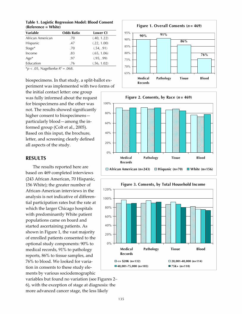
135

biospecimens. In that study, a split‐ballot ex‐periment was implemented with two forms of the initial contact letter: one group was fully informed about the request for biospecimens and the other was not. The results showed significantly higher consent to biospecimens—particularly blood—among the in‐formed group (Colt et al., 2005). Based on this input, the brochure, letter, and screening clearly defined all aspects of the study.  RESULTS

The results reported here are based on 469 completed interviews (243 African American, 70 Hispanic, 156 White); the greater number of African‐American interviews in the analysis is not indicative of differen‐tial participation rates but the rate at which the larger Chicago hospitals with predominantly White patient populations came on board and started ascertaining patients. As shown in Figure 1, the vast majority of enrolled patients consented to the optional study components: 90% to medical records, 91% to pathology reports, 86% to tissue samples, and 76% to blood. We looked for varia‐tion in consents to these study ele‐ments by various sociodemographic variables but found no variation (see Figures 2–6), with the exception of stage at diagnosis: the more advanced cancer stage, the less likely 

Table 1. Logistic Regression Model: Blood Consent (Reference = White) Variable Odds Ratio Lower CI African American .70 (.40, 1.22) Hispanic .47 (.22, 1.00) Stage* .70 (.54, .91) Income .83 (.65, 1.06) Age* .97 (.95, .99) Education .76 (.56, 1.02) *p < .05, Nagelkerke R2 = .068.

Figure 1. Overall Consents (n = 469)

90% 91%

86%

76%

65%

70%

75%

80%

85%

90%

95%

MedicalRecords

Pathology Tissue Blood

Figure 2. Consents, by Race (n = 469)

0%

20%

40%

60%

80%

100%

MedicalRecords

Pathology Tissue Blood

African American (n=243) Hispanic (n=70) White (n=156)

Figure 3. Consents, by Total Household Income

0%

20%

40%

60%

80%

100%

120%

MedicalRecords

Pathology Tissue Blood

<= $20K (n=132) 20,001-40,000 (n=114)

40,001-75,000 (n=103) 75K+ (n=110)

136

blood consent was obtained. This is not surprising in light of the fact that many patients are already undergo‐ing treatment by the time our inter‐view takes place. We entered these variables into a logistic regression model for blood consent, and those results are presented in Table 1. The bivariate association of consent with stage at diagnosis was significant, as was age. Older respondents were less likely to consent to give a blood sam‐ple.  

DISCUSSION

To date, the BCCC response rate is approximately 51%; the refusal rate is 43%. Two factors may be largely responsible for these rates. First, this is the first rapid case ascertainment study conducted by the Illinois De‐partment of Public Health. Most states, including Illinois, have cancer registries and typically mandate can‐cer reporting without patients’ con‐sent. So it is likely that few subjects who received information about the BCCC study from IDPH knew that cancer is a reportable disease and a cancer registry exists. In the modern‐day HIPAA environment, in which patients are sensitized to HIPAA rights at every physician and labora‐tory visit, HIPPA is a significant con‐cern that cannot be overlooked when trying to understand consent and co‐operation rates. Secondly, IDPH waits 45 days before mailing the initial study materials to eligible patients. Due to the detailed information we are collecting on their path to diagno‐sis, however, it is critical to the study design that the patients be interviewed as close to their diagnosis date as pos‐sible. But most breast cancer patients 

Figure 6. Consents, by Stage at Diagnosis

0%

20%

40%

60%

80%

100%

MedicalRecords

Pathology Tissue Blood

Stage 0 (n=119) Stage 1 (n=206)

Stage 2 (n=104) Stage 3/4 (n=28)

Figure 4. Consents, by Education

0%

20%

40%

60%

80%

100%

MedicalRecords

Pathology Tissue Blood

< HS (n=86) HS/GED (n=102)

Some college/college (n=209) Graduate work/degree (n=72)

Figure 5. Consents, by Age

0%

20%

40%

60%

80%

100%

MedicalRecords

Pathology Tissue Blood

<=48 (n=133) 49-55 (n=102) 56-65 (n=129) 66+ (n=105)

*p < .05

137

are already in treatment at the time they are in‐formed about the study; those with more ad‐vanced stages of disease may in fact be too ill to participate. Finally, once a subject declines par‐ticipation, we are not allowed to recontact them.  

Overall, our consent rates to the optional study elements, particularly the biospecimens, are respectably high, and we did not find any variation by race. Moreover, refusals to enroll in BCCC are similar by race. Our preliminary results suggest that once subjects decide to par‐ticipate in the study, they are comfortable con‐senting to all components, particularly since they knew what those components were at the time they enrolled. It is possible that those who refuse to enroll in the study are actually refus‐ing to these elements, a pattern found in an‐other study enrolling colorectal cancer patients in a genetics study (Ford et al., 2006; Evans, Stoffel, Balmana, Regan, & Syngal, 2006). How‐ever, our results are preliminary and represent only about half of the total number of com‐pletes expected in this study. Fortunately, we will have an opportunity to conduct a rigorous nonresponse analysis upon receipt of a de‐identified data file from IDPH that lists key demographics and stage of diagnosis for all women contacted for the study. We therefore will be able to control for the selection bias in the analyses presented here.  

REFERENCES

Colt, J. S., Wacholder, S., Schwartz, K., Davis, F., Graubard, B., & Chow, W. (2005). Response rates in a case‐control study: Effect of disclosure of biologic sample collection in the initial contact letter. Annals of Epidemiology, 15, 700–704. 

Eley, J. W., Hill, H. A., Chen, V. W., Austin, D. F., Wesley, M. N., Muss, H. B., et al. (1994). Racial differences in survival from breast cancer. Re‐sults of the National Cancer Institute Black/ White Cancer Survival Study. JAMA, 272, 947–954. 

Ford, B. M., Evans, J. S., Stoffel, E., Balmana, J., Regan, M. M., & Syngal, S. (2006). Factors asso‐ciated with enrollment in cancer genetics re‐search. Cancer Epidemiology Biomarkers & Prevention, 15, 1355–1359. 

Jacobellis, J., & Cutter, G. (2002). Mammography screening and differences in stage of disease by race/ethnicity. American Journal of Public Health, 92, 1144–1150. 

Moorman, P. G., Skinner, C. S., Evans, J. P., Newman, B., Sorenson, J. R., Calingaert, B., et al. (2004). Racial differences in enrollment in a cancer genetics registry. Cancer Epidemiology Biomarkers & Prevention, 13, 1349–1354. 

Murthy, V. H., Krumholz, H. M., & Gross, C. P. (2004). Participation in cancer clinical trials: Race‐, sex‐, and age‐based disparities. JAMA, 291, 2720–2726.

 

139

FEATURE PAPER: Challenges in Collecting Survey-Based Biomarker and Genetic Data: The NHANES Experience

Clifford Johnson, David Lacher, Brenda Lewis, and Geraldine McQuillan, National Center for Health Statistics

  

The use of direct physical measures is criti‐cal and necessary in order to estimate the extent of various diseases and risk factors for disease in the population. The use of such measures in clinical settings and interventions has occurred for many years. In recent years, there has been an increasing interest in collecting biological data in population‐based surveys.  

Biomarker data and other physical meas‐ures have been collected in the National Health and Nutrition Examination Survey (NHANES) since its beginning in 1960 (CDC/NCHS, n.d.). During these more than 45 years, numerous challenges have been encountered relative to the collection and laboratory processing of bio‐marker data. In recent years, the collection and processing of genetic specimens has been part of NHANES, and many lessons have been learned about the collection of this type of in‐formation in a general population‐based sur‐vey. The focus of this paper is to enumerate many of these challenges and describe the changes made to address these data collection and processing issues in NHANES.  

The origin of the NHANES is the National Health Survey Act of 1956, which formulated the need for national population surveys to assess the extent of illness and disabil‐ity in the U. S. population. The National Health Interview Survey (NHIS) was the first survey created to respond to this public health need and was first fielded in July 1957. For 50 years, this survey has been in continuous operation collecting data on health and illness of the popula‐tion using standardized in‐person household interviews.  

The need for additional data on health status that could best (or only) be assessed using direct physical measures 

also was recognized, and in 1958, planning for the first National Health Examination Survey began. An early decision was to collect these measures in a standardized environment; this led to the construction of mobile examination centers to collect this information. These centers could be moved from one location to another so that all data collected in the survey would util‐ize standard procedures and equipment. A lim‐ited set of biological specimens were included in the first NHES survey (NHES I) and in the subsequent survey on adolescents (NHES III) (Table 1). There were no biological tests done on children who participated in the NHES II sur‐vey (Table 1). 

In 1971, a nutrition component was added to the NHES, and the survey became known as the National Health and Nutrition Examination Survey (NHANES). The number of biomarkers collected in NHANES I (1971–1975) was much greater than the number collected in any of the three NHES surveys in the 1960s. In addition, the survey covered a much wider age range (1–74 years) than any of the previously conducted NHES surveys. Tests were completed on whole blood, serum, and urine samples. Some of the 

Table 1. Laboratory Tests in NHES I, NHES II, & NHES III TEST I II III I. Hematological Assessments

a. Hematocrit b. Red blood cell antigens

II. Serum Biochemical Assessments a. Cholesterol, total b. Glucose c. Protein bound iodine d. Plasma proteins

III. Syphilis Screening IV. Bacteriuria V. Urine Assessments

a. Urine sugar b. Urine albumin

140

new biomarkers were added to address specific nutrition issues, but others were added to pro‐vide national reference data for selected immu‐nization and infectious disease assessments (Table 2).  

The expansion of the number of biomarkers collected in NHANES I was accompanied by an increase in the number of data collection and methodological issues associated with these 

laboratory assessments. There were limited quality assurance procedures in the field during specimen collection and in the laboratories dur‐ing testing. There were also delays in coding and processing the results. These factors made it impossible to release various test results be‐cause issues of data quality and interpretation could not be addressed in a timely manner. In addition, the expansion of the survey to include 

Table 2. Laboratory Tests in NHANES I, NHANES II, HHANES, & NHANES III TEST I II H III TEST I II H III I. Hematological Assessments II. Serum Biochemical Assessments (cont’d)

a. Sedimentation rate q. Carotene profile b. Differential smears r. Cotinine c. Hematocrit s. Bile salts d. Hemoglobin t. Pesticides e. Cell counts u. Syphilis serology f. Neutrophil hypersegmentation v. Hepatitis A & B serology g. Mean cell volume w. Tetanus h. Red cell distribution width x. Diphtheria, rubella, polio

II. Serum Biochemical Assessments y. Herpes simplex I & II a. Folic acid z. IgE b. Iron & total iron-binding capacity aa. Human immunodeficiency virus c. Vitamin C bb. C-reactive protein d. Vitamin D (25-hydroxy D) cc. Rheumatoid factor e. Zinc & copper dd. Follicle stimulating hormone f. Vitamin A ee. Luteinizing hormone g. Vitamin B-12 ff. Thyroxine (T4) h. Plasma glucose (GTT) gg. Thyroid stimulating hormone (TSH) i. Selenium hh. Antithyroglobulin antibodies j. Cholesterol, total ii. Antimicrosomal antibodies k. HDL & LDL cholesterol jj. Insulin l. Triglycerides kk. C-peptide m. Apolipoproteins Al & B ll. Plasma fibrinogen n. Total & ionized calcium III. Whole Blood Biochemistry Assessments o. Ferritin a. Protoporphyrin p. Biochemistry profile: b. Lead

1. Total carbon dioxide c. Folate 2. Blood urea nitrogen d. Carboxyhemoglobin 3. Total bilirubin e. Glycosylated hemoglobin 4. Alkaline phosphatase f. Priority toxicant volatiles 5. Cholesterol IV. Urinary Assessments 6. SCOT, AST a. Urinalysis 7. SGPT, ALT b. Pesticides 8. LDH c. Riboflavin 9. Total protein d. Thiamin

10. Albumin e. Cadmium 11. Creatinine f. Creatinine 12. Glucose g. Microalbumin 13. Calcium h. Urinary iodine 14. Chloride i. Pregnancy test 15. Uric acid j. Priority toxicant phenols 16. Phosphorus V. Excess and Reserve Vials 17. Sodium a. Serum 18. Potassium b. White blood cells for DNA banking

141

young children proved to be problematic be‐cause of a high number of refusals for the venipuncture or unsuccessful blood draws even with acceptance of the venipuncture. An early lesson learned was the need to have phleboto‐mists that were skilled in drawing blood on children. Making this a requirement for the po‐sition resulted in a drop in missing data from 70% to about 30%.  

Other challenges and problems occurred in the laboratory in the NHANES mobile exami‐nation center in NHANES I. Numerous vials were lined up next to each other in racks after aliquots of serum had been processed. The vial to be used for serum folate testing was placed next to the vial for vitamin C testing. The preparation of the serum folate vial (according to the protocol) required the addition of a “pinch of ascorbic acid” to the tube. Lab techni‐cians did not put a stopper in the vitamin C vial before adding the pinch of ascorbic acid to the folate vial. The result was numerous abnor‐mally high vitamin C levels that were not physiologically possible in the population. Thus, the entire set of data for vitamin C was deemed unusable and never released. 

NHANES II (1976–1980) brought increased numbers of biomarkers and the first environ‐mental assessments (blood lead and selected pesticides) (Table 2). As in NHANES I, methodo‐logical issues related to data collection protocols and laboratory methodologies were encoun‐tered. For example, vials that were thought to be free of environmental contaminants turned out not to be, and various environmental assess‐ments collected in the course of NHANES II were declared methodologically unsound and never released. These protocol and equipment problems were corrected prior to the fielding of NHANES III. 

During the course of data collection in NHANES II, a practical and fiscal decision was made to change the laboratory method for se‐rum folate and red blood cell folate from a microbiological method to a more automated radioimmunoassay method. However, the two 

folate lab methods did not produce comparable results at all levels of values. Thus, upon review of the raw data (after the survey was com‐pleted), an expert panel determined that the data from the two folate lab methods could not be combined. Thus, the ability to calculate na‐tional reference data for serum and red cell folate was not possible (Life Sciences Research Office, 1984). This example (and a few others) led to crossover studies being conducted with method changes (whenever possible) in all NHANES surveys since that time. These cross‐over studies are an important component of blood and urine specimen testing protocols and are critical for analyses that are conducted to address time trends. 

The number of blood and urine biomarkers included in NHANES III (1988–1994) increased significantly from the number of biomarkers in NHANES II (Table 2). This occurred for two reasons. First, many new laboratory methods had been developed that used less volume of serum or plasma; thus, more assessments could be included in the survey without increasing the volume of blood collected from each person selected for the survey. The second reason for the increase in the number of lab assessments was the availability of a variety of new lab methods. So, as the overall content and com‐plexity of NHANES grew, so did the use of blood and urine specimens to address a wide array of public health issues. 

This expansion in the number of laboratory biomarkers significantly increased the complex‐ity of survey operations and specimen collec‐tion. The number of vials of serum increased, requiring increased staff to process the speci‐mens in the field. The need to ship over 100,000 vials of blood per year to numerous labs around the country using dry ice added further logistical challenges. Collecting and shipping large numbers of lab specimens is a significant impediment to the inclusion of biomarkers in population‐based surveys.  

Another significant change in the number of laboratory assessments occurred with the 

142

implementation of the ongoing and continuous NHANES beginning in 1999. The development of numerous environmental lab assays in‐creased the total number of lab biomarkers by tenfold, with little increase in the volume of blood and more utilization of urine than in pre‐vious surveys. 

In addition, DNA specimens were added back into the survey with additional consent language that separated consent for the general survey and lab biomarkers from the stored bio‐logic specimens that include serum, plasma, urine and DNA specimens. Survey participants could agree to (or refuse) all of the lab bio‐markers, agree to or refuse the planned use of stored biologic specimens, and agree to or refuse the collection and use of the DNA specimens. This has resulted in a much more complicated administrative responsibility for NHANES staff with respect to use of lab biomarkers. 

In addition to administering the continuous survey, the NHANES staff administers an in‐vestigator‐driven research program where re‐searchers can submit proposals for the stored samples on an ongoing basis. These proposals must undergo both technical and ethics review before specimens that have been stored from consenting participants can be used for these re‐search projects. The availability of these speci‐mens, though, has greatly increased the research potential of the survey with the addition of over 20 additional laboratory data sets in the past ten years. 

More recently, a separate process was de‐veloped for the use of the NHANES III DNA specimens; it currently is being adapted for use with the NHANES 1999–2002 DNA specimens. The collection of DNA specimens in NHANES has had many challenging issues. Although in‐formed consent was acquired from each survey participant during the 1991–1994 time period for which the specimens were collected, by the time the survey was completed and the samples prepared for analysis, the Ethics Review Board ruled that the original informed consent was not adequate for genetic research and that the 

specimens could only be used in an anonymous fashion and not linked to most of the other NHANES III data. The restriction of anonymi‐zation greatly reduced the usefulness of the NHANES phenotypic data; thus, for a number of years, the NHANES III DNA was not util‐ized. After the publication of the Report and Rec‐ommendations of the National Bioethics Advisory Commission in August 1999 on research involv‐ing human biologic materials (National Bioethics Advisory Committee, 1999), the NHANES pro‐gram obtained Ethics Review Board approval to link the genetic data with other survey data in a controlled and restricted data access environ‐ment (the NCHS Research Data Center). A simi‐lar approach is being utilized for the NHANES 1999–2002 DNA samples collected in this sub‐sequent time period.  

Throughout the 46 years of collection of laboratory biomarkers in NHANES, a number of other general issues have arisen. Some of these are summarized below. 

One of the most significant of these issues is the problem that occurs when an existing labo‐ratory method is discontinued and a new method is substituted for a particular assay. How and when to conduct crossover studies (to compare the two methods) is an important de‐cision (and critical to the use and interpretation of the data). For NHANES, there are instances where these types of studies did not occur, and we were unable to determine whether changes over time were real, methodological, or both. Even if a crossover study is conducted, there may be inadequate sample sizes for the study; this can lead to difficulties knowing the rela‐tionship of the two methods at the “tails of the distribution.” On many occasions, that is the area of greatest public health significance, and the lack of an adequate crossover study can re‐sult in uncertain interpretation of results. 

In our NHANES experience, we learned that the use of blind quality control specimens is critical. Even though most labs have internal quality control procedures in place, there is the chance that the lab is “not in control,” and the 

143

only way to monitor that possibility is by send‐ing blinded split‐sample specimens to the lab. The lab and lab technicians do not know which of the specimens are of this type. They are aware of their own internal quality assurance control specimens, and that knowledge can in‐fluence their handling and processing proce‐dures. Over time, the NHANES program has found quite a few instances where these blind quality control specimens were the only way that problems in laboratory procedures were discovered and corrected.  

Another issue is the ethical responsibility to report results to sample persons who partici‐pate in the survey. This requires timely analysis and reporting of results from labs to NCHS and then timely reporting of these results to partici‐pants by NHANES program staff. In addition, there needs to be some agreed‐upon clinical cutpoints that can be utilized in the reporting of the results. If there are no agreed‐upon clinical criteria for abnormal values, then results are not reported to individual participants. There is an ongoing responsibility to review new informa‐tion to determine whether a lab result that was not reportable in the past is now reportable.  

This reporting of findings in a timely man‐ner influences what lab tests may be done on stored specimens at a later point in time. The NHANES program along with the survey’s Eth‐ics Review Board has decided that any report‐able lab biomarker will not be done on stored specimens because the subject could have been examined many years earlier, and later report‐ing of a clinically significant biomarker is prob‐lematic. The assessment of what research laboratory tests may be clinically significant biomarkers has been a challenge. Thus, to date, most research on NHANES stored specimens has been for new and emerging biomarkers that do not have established clinical cutpoints. In spite of this limitation, many stored specimen biomarker proposals have been approved for previous NHANES surveys, and the results have been released on public use data files. 

The recent development of biomarker tests that can utilize blood from a finger stick or from a saliva sample will make the inclusion of these assessments more feasible for household‐based population surveys. The challenge faced with this approach is whether the laboratory meth‐ods that utilize these samples produce compa‐rable results to the traditional blood sample. In many cases, the answer to this question is not known yet. If these less invasive tests prove comparable and reliable, the potential for col‐lecting biomarkers in other surveys increases dramatically. Even so, there remain many logis‐tical complications for any household‐based survey attempting to collect biomarkers and genetic data. Training interviewers to be phle‐botomists is much more difficult than training phlebotomists to be interviewers. In some cases, it may require an interviewer and phlebotomist team to successfully collect both interview and biomarker data in the home. This option would result in significant cost increases for survey operations (let alone the numerous issues re‐lated to handling of blood and urine specimens in a household setting). Even if interviewers can be trained to collect blood from a finger stick, standardization of collection procedures and handling of specimens remains a signifi‐cant operational constraint. In the case of NHANES, the mobile examination center with a lab and lab staff has remained the mode for biomarker data collection for the entire history of the survey.  

In summary, the collection of biomarkers and genetic data in population‐based surveys is a significant challenge. The issues include how to obtain informed consent, what staff to use to collect and process the biomarkers, how to col‐lect and process the specimens in a timely man‐ner, how to select a laboratory and lab method, and how to implement quality assurance proce‐dures to ensure that the results will be valid and interpretable. Over the 46 years that biomarkers have been collected, processed, and analyzed in NHANES surveys, almost every logistical and methodological complication that can occur has 

144

occurred. These challenges continue to occur because science moves on, methods change, and people do not always foresee what might occur in a real‐time survey operation. The im‐portant lesson is to learn from mistakes (and successes) and to use this knowledge in future surveys.  

 REFERENCES

Centers for Disease Control and Prevention, Na‐tional Center for Health Statistics. (n.d.). National Health and Nutrition Examination Survey. Re‐trieved August 17, 2007, from www.cdc.gov/nchs/nhanes.htm 

Life Sciences Research Office. (1984, October). As‐sessment of the folate nutritional status of the U.S. population based on data collected in the second Na‐tional Health and Nutrition Examination Survey, 1976–1980. Rockville, MD: Federation of Ameri‐can Societies for Experimental Biology.  

National Bioethics Advisory Commission. (1999). Research involving human biological materials: Ethi‐cal issues and policy: Vol. 1. Report and recommen‐dations of the National Bioethics Advisory Commission. Rockville, MD: Author. Retrieved August 17, 2007, from http://bioethics.georgetown.edu/nbac/hbm.pdf

    

145

FEATURE PAPER: Incorporating Biomarkers for the Fourth Wave of the National Longitudinal Study of Adolescent Health

Amy Ladner, RTI International   

INTRODUCTION

The National Longitudinal Study of Ado‐lescent Health (Add Health) is a study of a na‐tionally representative sample of more than 20,000 individuals who were in grades 7–12 in 1994–1995. Since the initial in‐school question‐naires were administered, these sample mem‐bers have been followed through adolescence and the transition to adulthood with three in‐home interviews. This landmark study was de‐signed by a nationwide team of multidiscipli‐nary investigators from the social, behavioral, and health sciences led by researchers at the University of North Carolina and funded by the National Institute of Child Health and Human Development with cofunding from 17 other federal agencies (Harris, 2006). Plans for a fourth in‐home interview with respondents who will be 24–32 years old currently are un‐derway, with a pretest of 300 sample members slated to start in April 2007.  

Given the size and spread of the Add Health sample and the nonclinical setting of our inter‐views, we have chosen methods to collect bio‐logical data that are noninvasive, innovative, cost‐effective, and practical for population‐level research. As we plan and move into Add Health Wave IV data collection, we recognize the in‐herent challenges in collecting numerous bio‐markers and other health data in a field setting. This paper will document the extensive prepa‐ration, interviewer training, and specimen tracking system development required to en‐sure the study’s success.   OVERVIEW OF ADD HEALTH WAVE IV

Data to be collected at Wave IV from ap‐proximately 17,000 participants include • Social and economic status, behaviors, and 

experiences; 

• Psychological status and experiences; • Reported health status and health behaviors; • Environmental contexts (residence, college); • Spatial location of residence; and • Extensive biomarkers, including physical 

measurements, blood pressure, lipids pro‐file, DNA, and other measures of chronic stress, metabolic syndrome, and immune function (Harris, 2005). 

 

Wave IV will focus on three major health concerns for the Add Health cohort: (1) obesity, (2) health risk behavior, and (3) stress (Flegal, Carrol, Ogden, & Johnson, 2002; McEwen, 1998; Schulenberg, Maggs, & Hurrelmann, 1997). These were selected due to the prevalence of young adults in the population and the wide‐spread consequences for adult health and well‐being. With the addition of data and bio‐markers collected in Wave IV, we will be able to examine the factors contributing to obesity, in‐vestigate the consequences of longer exposures to risky lifestyles on health status, and link sources of chronic stress in the early stages of the life course to subsequent life course trajecto‐ries of cumulative physiological risk.  ADD HEALTH WAVE IV BIOMARKER COLLECTION

The choice of biological data for Wave IV is driven by scientific knowledge of the leading causes of health at this and future developmental stages of the Add Health cohort, the role of spe‐cific biological processes in causation, and the ability of specific measures to characterize these processes. We plan to collect biological data on anthropometric, cardiovascular, metabolic, immune function, and inflammatory processes that capture important health conditions asso‐ciated with obesity, chronic stress, and poor health behaviors, as well as critical markers of 

146

future health risks, such as diabetes, cardiovas‐cular disease, coronary artery disease, physical and cognitive decline, poor kidney functioning, and early mortality. Within these scientific cri‐teria, the choices of biological measures were constrained by the feasibility, validity, and reli‐ability of methods used to obtain biological specimens in a nonclinical setting. Table 1 lists the domains of biological measures that will be collected during Wave IV.  

 DATA COLLECTION SEQUENCE & MEASURES

Data and specimen collection during the in‐terview will follow the sequence presented in Figure 1. Collection protocols and intervening rest periods are designed to maximize efficiency in obtaining informed consent and minimize pu‐tative carryover effects. Total time to collect all biological specimens and measurements is 40 minutes. We also will ask respondents to self‐collect three saliva samples the day following the interview for cortisol assay.   Anthropometric Measures

As in earlier waves, trained and certified in‐terviewers will measure the weight and height of Wave IV participants who are dressed, have removed their shoes, and are standing on an un‐carpeted floor (where possible). Weight will be 

measured to the nearest 0.2 pound using the Tanita HD 351 Weight Scale (max: 440 lb). Height will be measured to the nearest 0.25 inch using a carpenter’s square, tape measure, and Post‐it® note. Arm and waist circumference will be measured to the nearest 0.25 inch using a Seca 200 circumference tape measure (max: 78 in). Arm circumference will be used to guide selection of an appropriately sized blood pres‐sure cuff. Waist circumference will be measured midway between the lowest rib and the supe‐rior border of the iliac crest at end‐expiration. Body mass index will be calculated from weight and height and interpreted in accordance with Clinical Guidelines on the Identification, Evalua‐tion, and Treatment of Overweight and Obesity in Adults—The Evidence Report (NIH, 1998). 

 Cardiovascular Measures

Trained and certified interviewers will measure the pulse and systolic and diastolic blood pressure of participants and key the re‐sults into the computer according to a standard‐ized protocol. Participants will be asked to avoid caffeinated beverages and foods, heavy physical activity, smoking, and alcohol for eight hours prior to the interview. Compliance with these requests will be recorded in the questionnaire along with other factors known to affect blood 

Table 1. Add Health Wave IV Domains of Biological Measures

Domain Specimen Measure Anthropometric Height, weight, BMI, arm & waist circumference Cardiovascular Blood pressure, pulse rate, pulse pressure, mean arterial pressure Metabolic Dried blood spots Lipid panel, glycosylated hemoglobin Inflammation Dried blood spots C-reactive protein Immune function Dried blood spots, saliva Epstein-Barr virus antibodies, cortisol DNA Saliva Candidate gene loci & SNP panels Kidney function Urine Microalbumin, creatinine

Figure 1. Biomarker Data Collection Sequence during Interview

147

pressure and/or pulse (medication use, time of day). After a five‐minute quiet rest period, seated values of SBP, DBP (mmHg), and pulse (beats/min) will be automatically recorded to the nearest whole unit using an appropriately sized cuff and the Microlife 3MC1‐PC_IB digital oscil‐lometric blood pressure monitor. Three serial determinations will be performed from the right arm (when possible) at 30‐second inter‐vals. Pulse pressure and mean arterial pressure will be estimated indirectly. The computer will automatically calculate, store, and display the average of the last two determinations for the purpose of classifying, reporting, and guiding follow‐up according to current guidelines from the Joint National Committee on Prevention, Detection, Evaluation, and Treatment of High Blood Pressure (Chobanian et al., 2003). After an interview has been completed, interviewers will connect the blood pressure monitor to the computer via USB interface to download the readings. 

 Urine Collection

Microalbuminuria (MA) above 20mg/dL may be an early marker of renal disease. To evaluate MA incidence and prevalence in Wave IV respondents, participants will be asked to provide a random first stream sample of 15 cc. Samples will be packed in insulated coolers with frozen gel packs and shipped to the UNC Kidney Center (Chapel Hill, NC) for analysis.  

 Finger-Prick Dried Blood Spots

Trained and certified interviewers will use finger prick to obtain 10 blood spots (750–800 μL) for dry spot assays of lipid panel, hsCRP (mg/L), HbA1c (%), EBV antibodies, and calcu‐lated glucose. Compared to venipuncture, fin‐ger prick is a relatively convenient, inexpensive, and noninvasive means of collecting whole blood. Prior to collecting blood spots, inter‐viewers will ask participants to warm their hands in very warm water for approximately 

one minute. Interviewers then will obtain whole blood spots by (1) cleaning each partici‐pant’s middle or ring finger with isopropyl al‐cohol; (2) applying a restriction band to the middle of the upper arm; (3) pricking the se‐lected finger with a sterile, disposable micro‐lancet (Microtainer, Franklin Lakes, NJ); (4) wiping away the first formed drop; (5) placing three drops of blood via capillary action onto standardized filter paper (Biosafe Laborato‐ries, Chicago, IL) to obtain dry spot assays for lipid panel, HbA1c (%) and calculated glucose (mg/dL); and (6) placing seven additional drops via capillary action onto standardized filter paper (Whatman #903, Florham Park, NJ) for dry spot assays of hsCRP (one spot), EBV anti‐bodies (one spot), and potential future re‐search (five spots). If one finger prick does not produce at least five drops of blood, the inter‐viewer will perform a second finger prick after participant consent. Blood spots will be air dried per manufacturer instructions (Biosafe—15 minutes, Whatman—4 hours) and then placed in plastic bags with desiccant (Humid‐ity Sponge, VWR) for transport to the labora‐tory performing the assays (lipid panel—Biosafe Laboratories, Chicago; hsCRP—UWMC Immu‐nology Lab, Seattle).  Saliva Collection—DNA

In collaboration with the Institute of Behav‐ioral Genetics in Boulder, Colorado, Add Health will collect, extract, quantify, and store DNA samples from all participants in Wave IV. Genotyping will consist of evaluations of Variable Number Tandem Repeat, Short Tandem Repeat, Single Nucleotide Polymorphism (SNP) or hap‐lotype blocks that will be defined by a panel of SNPs. Genomic DNA will be isolated from sa‐liva samples using the Oragene commercial col‐lection kit (DNAgenotek). The DNA is collected from 2 ml of saliva without swabbing the inside of the cheeks. 

 

148

Saliva Collection—Cortisol

Add Health participants also will be asked to self‐collect three saliva samples for cortisol assay the day after the interview (at awakening, 30 minutes later, before bed) using a 2 ml cryo‐tube (Wheaton Science Products, Millville, NJ) and soda straw. Interviewers will instruct par‐ticipants to place one end of the straw into the cryotube and one end into their mouth to push saliva through the straw into the tube until the saliva reaches the fill line (1 ml) and have them practice collecting a sample during the inter‐view. The interviewer also will instruct the par‐ticipant to complete a short checklist following each collection. The checklist is a brief ques‐tionnaire designed to collect relevant informa‐tion about protocol adherence and stressors experienced on the day of collection. The inter‐viewer then will give the saliva collection kits, instructions, checklists, and shipping materials with an addressed prepaid envelope to each participant. Saliva samples will be sent to Sali‐metrics LLC in State College, PA. 

For the pretest, the cryotubes will be given to the participant stored inside a medication bottle with a MEMS6 TrackCap (Aardex, Swit‐zerland)—a lid containing a microelectronic chip that accurately records the date and time of day that the lid is opened to retrieve a cryotube. Opening times will be used as proxies for sam‐ple collection times. In addition, participants will be divided into three groups and told ei‐ther (1) that saliva collection is time‐stamped, (2) that saliva collection is time‐stamped for randomly selected participants, or (3) nothing about whether saliva is time stamped. Using this design, we will estimate the difference be‐tween participant‐reported and TrackCap‐recorded sample collection times.  

OVERCOMING CHALLENGES TO BIOMARKER COLLECTION

EXTENSIVE PLANNING

The choices of biological measures to collect in Wave IV were constrained by the feasibility, validity, and reliability of methods used to ob‐tain biological specimens in a nonclinical setting by nonmedically trained individuals. In order to determine the collection methods and equip‐ment needed to collect biomarkers for Wave IV, we built an extensive planning period into the project schedule (Table 2). This planning period provided the necessary time needed to examine and test various pieces of equipment, investigate federal and state regulations regarding shipping biological specimens and education require‐ments for personnel collecting blood spots by finger prick, explore newer technologies for col‐lection and analysis of biomarkers, and convene a panel of experts—the Add Health National Biomarker Advisory Committee—for peer re‐view and advisory inputs. 

The planning period provided an invaluable opportunity for us to alter protocols and equip‐ment needs based on cost and feasibility of col‐lecting measures and biomarkers in the home setting and allowed us to add protocols to measure cardiovascular response to a mental stress test and biomarker reliability. Initially, we planned to measure height with a stadiometer (Seca 214 Road Rod), perform wet blood spot lipid panel analysis with a portable cholesterol monitor (CardioChek PA), and collect saliva for cortisol assay using Salivettes (Salimetrics, State College, PA). After examination of the stadi‐ometer, we decided to alter the height protocol and measure height with a carpenter’s square and tape measure to ease interviewer burden (the stadiometer weighed six pounds, did not 

Table 2. Timeline for Wave IV Data Collection Task Start Date Stop Date Time Plan and prepare for pretest May 2006 Mar 2007 11 months Conduct pretest Apr 2007 May 2007 2 months Revise questionnaire and plan for main study Jun 2007 Dec 2007 7 months Conduct main study Jan 2008 Sep 2008 9 months

149

fit into the interviewer rolling backpack, and required in‐home assembly) and save costs. We also altered the finger‐prick protocol to perform all blood spot assays on dry spots to ease inter‐viewer burden. To perform wet blood analysis on a portable cholesterol monitor would re‐quire interviewers to fill one 40 μL capillary tube with blood for lipid panel analysis, fill one 15 μL capillary tube with blood for glucose analysis, place the collected blood on dispos‐able test strips, wait for the analyzer to run one test strip before inserting the second test strip (lipid panel strip analysis required three min‐utes to run), and collect seven remaining blood spots onto standardized filter paper. After a lit‐erature review and meeting with the Add Health National Biomarker Advisory Commit‐tee, we also decided to collect saliva for cortisol assay with 2 ml cryotubes and soda straws. 

In addition to making equipment and proto‐col changes during the planning period, we added a protocol and study to Wave IV. Follow‐ing the blood pressure protocol in the interview, we administer a backward‐digit‐span series, ask‐ing the respondent to repeat a set of numbers back to the interviewer in the reverse order. For example, if the interviewer listed “2, 4,” the re‐spondent would reply “4, 2,” with the series progressively increasing in length. After comple‐tion of the backward‐digit span, the interviewer performs two additional blood pressure read‐ings 30 seconds apart to measure cardiovascular response to a mental stress test. We also added an Intra‐individual Variation Study to Wave IV to estimate the reliability and validity of the biomarker data collected in the field. To this end, we will administer a shortened interview within two weeks of the initial interview to 50 partici‐pants in the pretest and 50 participants in the main study and collect all biological measures and samples. We will use the intraclass correla‐tion coefficient as a measure of reliability for monitoring both the collection and processing of biomarkers collected in Wave IV and for quality assurance and control purposes. 

STANDARDIZING COLLECTION PROTOCOLS

To ensure that the biological data collected in Wave IV are unbiased and valid, we incorpo‐rated standardization and quality control prac‐tices into biomarker collection protocols, interviewer training protocols, and weekly communications with the interviewers and labo‐ratories. Collecting high‐quality biological data starts with hiring interviewers with previous ex‐perience collecting biological measurements and samples. For the Wave IV pretest, 15 of the 24 in‐terviewers hired to date have previous experi‐ence collecting biomarkers and/or biological measures or blood pressure. Before any inter‐viewer may collect data in the field, he or she must attend a weeklong training and pass a rig‐orous certification conducted at the conclusion of the training. During training, interviewers are instructed on collecting each measurement and sample; given a comprehensive training guide that lists step‐by‐step instructions and pictures for completing each biomarker protocol and for labeling, packing, and shipping the samples to the appropriate laboratories; and given multiple opportunities to practice each protocol in both scheduled training mocks and after‐hours study halls. Once interviewers have passed certifica‐tion and begin collecting data, we maintain weekly communication with them regarding the quality of specimens collected in the field. We will receive daily reports from the laboratories that not only confirm sample receipt but also list any problems with specimen quality (e.g., blood spot did not completely soak through the filter paper, specimen leaked during transit). We will address these problems immediately and retrain interviewers on particular biomarker protocols if needed.  

 MONITORING EQUIPMENT FUNCTION

We also built quality control measures into biomarker protocols by monitoring equipment function. On a weekly basis, interviewers will perform and document calibration of the digital scales by first weighing themselves, weighing 

150

their laptops, and then weighing themselves holding their laptops. If the combined weight does not match the summed value and differs by more than one pound, interviewers will notify their supervisor and have the scale replaced. We also incorporated monitoring equipment func‐tioning of the blood pressure monitor into the programming of the interview and in post‐interview processing. During the interview, if the blood pressure monitor returns an error message or malfunctions (does not settle on a reading after the cuff deflates), the interviewer will enter this information in the computer. If this problem is experienced three times during an interview, a note appears on the computer screen alerting the interviewer to discontinue use of the monitor and contact his or her super‐visor to have the monitor replaced. We also can observe blood pressure monitor function across interviews by examining the number of mal‐functions recorded by a particular interviewer for a specific period of time. Based on the type of error message received and the frequency of malfunction, we can assess whether the prob‐lem is with the interviewer or the equipment and address it as appropriate.   TRACKING SYSTEMS

Collecting and shipping biological samples across the country via multiple couriers so that samples arrive within acceptable timeframes and at appropriate temperatures requires an auto‐mated tracking system, standardized commu‐nication protocols, and active involvement by the interviewers, field supervisors, project staff, and laboratory personnel. Since each sample requires a specific packing scheme, interview‐ers will not only be trained and certified on packing each specimen but also will have ready access to written packing instructions and pho‐tographs of correctly packed samples in their Job Aids booklet. (Written instructions also will be programmed into the questionnaire.) During the interview, interviewers will scan the bar‐code on each specimen’s shipping label using a handheld barcode wand attached to the laptop 

via USB interface. This includes not only the la‐bels for the specimens that the interviewers will be delivering to Federal Express (blood spots, DNA, urine) but also the barcode tracking number of the U.S. Postal Service (USPS) label for the cortisol sample that the participant will mail after self‐collection. These tracking num‐bers, as well as the interview date, will popu‐late the report of specimens that should be arriving at the laboratories. We also developed reports that capture specimens received by the labs and delinquencies (specimens shipped to the lab but yet reported as received).  

Once we have the tracking numbers associ‐ated with the shipments to the labs, we can use the online tracking mechanisms provided by Federal Express and USPS to verify delivery prior to lab notification of receipt. We developed an interface that pulls shipment tracking data from Federal Express and USPS into our reports without manual entry of tracking numbers by project staff. As part of Wave IV communication protocol, the majority of participating laborato‐ries report specimen receipt within one week of arrival and upload receipt reports to the secure file server. Our tracking system then automati‐cally compares the list of specimen IDs we ex‐pect to be received with the Federal Express and USPS tracking mechanisms and reports of re‐ceipted specimens by the labs and identifies de‐linquent specimens. Delinquency is defined by the type of courier service to the laboratory (Ta‐ble 3). For specimens shipped via Federal Ex‐press, a specimen is considered delinquent if we have not received report of receipt four days af‐ter collection. For specimens shipped through USPS, specimens will be considered delinquent if we have not received report of receipt seven days after interview. Project staff will follow up all specimens identified as delinquent with the following order: (1) courier, (2) field supervisor/ interviewer, and (3) lab. We also will make fol‐low‐up calls to participants who agreed to pro‐vide the cortisol sample but whose samples did not arrive at the lab. 

151

CONCLUSION

As we move into the pretest for Add Health Wave IV, we understand the challenges in col‐lecting numerous biomarkers and health meas‐ures in a nonclinic setting by nonmedically trained interviewers. While researchers at the University of North Carolina have been plan‐ning this data collection effort since the conclu‐sion of Wave III in 2002, under this contract we have spent a year investigating equipment and collection methodologies that are noninvasive, cost‐effective, and feasible for population‐level research; developing biomarker collection proto‐cols that will result in high‐quality, reliable data; and building an automated specimen tracking system that will allow us to manage 85,000 shipments from almost 300 interviewers to mul‐tiple laboratories across the U.S. Interviewer training and certification on each health meas‐urement and biomarker collection protocol is es‐sential to the study’s success in incorporating standardized, unbiased biological data with pre‐existing longitudinal Add Health data. At the conclusion of Add Health Wave IV, we will be able to provide unique opportunities to study linkages in social, behavioral, environmental, and biologic processes that lead to health and achievement outcomes in young adulthood. 

 

REFERENCES

Chobanian, A. V., Bakris, G. L., Black, H. R., Cush‐man, W. C., Green, L. A., Izzo, J. L., Jr., et al. (2003). National High Blood Pressure Education Program Coordinating Committee. The seventh report of the Joint National Committee on Pre‐vention, Detection, Evaluation, and Treatment of High Blood Pressure (JNC7). Hypertension, 42, 1206–1252. 

Flegal, K. M., Carrol, M. D., Ogden, C. L., & Johnson, C. L. (2002). Prevalence and trends in obesity among U.S. adults. JAMA, 288, 1723–1727. 

Harris, K. M. (2005). The National Longitudinal Study of Adolescent Health (Add Health) Wave IV: Social, behavioral and biological linkages. Overview of pro‐gram project for Add Health Wave IV. Chapel Hill, NC: Carolina Population Center.  

Harris, K. M. (2006, August). Add Health Wave IV. So‐cial, behavioral, and biological linkages. Presented at the Add Health Biomarker Advisory Committee Meeting, Chapel Hill, NC. 

McEwen, B. S. (1998). Stress, adaptation and disease: Allostasis and allostatic load. Annals of the New York Academy of Sciences, 840, 33–44. 

NIH (National Institutes of Health). (1998). Clinical guidelines on the identification, evaluation, and treatment of overweight and obesity in adults—The evidence report. Obesity Research, 6(Suppl. 2), 51S–209S. 

Schulenberg, J., Maggs, J. L., & Hurrelmann, K. (1997). Negotiating developmental transitions during adolescence and young adulthood: Health risks and opportunities. In J. Schulen‐berg, J. L. Maggs, & K. Hurrelmann (Eds.), Health risks and developmental transitions during adolescence (pp. 1–19). Cambridge, UK: Cam‐bridge University Press.

 

Table 3. Specimen Delinquency, by Courier & Sample

Specimen Status by Day

Federal Express (DNA, blood spots for hsCRP, EBV, urine)

Federal Express (blood spots for lipid panel)

USPS (salivary cortisol)

Interview Samples collected, shipped Sample collected, shipped Interview 2 Specimen arrives at lab Specimen arrives at lab Samples collected 3 Receipt reported Sample processing Shipped 4 Results and receipt reported In transit 5 Sample arrives at lab 6 Receipt reported

 

153

FEATURE PAPER: Ethical, Legal, and Social Concerns When Collecting Biospecimen Data Linked to Individual Identifiers

Barbara Koenig, Mayo College of Medicine    Paper not submitted.

 

155

SESSION 3 SUMMARY Alisha D. Baines, VA Medical Center of Minneapolis

Michael Davern, University of Minnesota   

The floor discussion following the Session 3 presentations focused on three major areas: preparation and collection of biomeasures in practice, data quality issues associated with the addition of biomeasure collection, and issues surrounding consent.  

PREPARATION & COLLECTION OF BIOMEASURES IN PRACTICE

Preparing for biomeasure collection re‐quires consideration of the amount of materials field interviewers will need to carry. While the study described by Smith and colleagues did not involve the transport of chairs, a Chronic Obstructive Pulmonary Disease (COPD) study had two interviewers conduct each interview because of the need to bring along a host of re‐quired equipment, such as a folding table and chair, to the respondent’s home for measure‐ment. Smith indicated that a great deal of thought went in to what materials to use and how to best transport them to respondent households. For more basic measures, such as height, it was more efficient to use a tape measure than more standard medical equip‐ment for measuring height. For measures that involved specimen collection, there was con‐sideration of how to move clinical measures into the home. The goal was to get as close to the gold standard as possible but still take into account the portability and robustness of the materials. The equipment was tested ahead of time and was researched to see if it had been tested before and whether it was FDA ap‐proved, and the manufacturer’s reliability data was reviewed. Further, a pilot period was use‐ful for testing equipment and collection proce‐dures.  

DATA QUALITY ISSUES ASSOCIATED WITH THE ADDITION OF BIOMEASURE COLLECTION

The addition of biomeasure collection to the survey research process brings about a con‐comitant increase in the potential for error. Along with the usual sources of survey error, there also is error associated with the collection and shipment of biological specimens and laboratory error. Such errors can be the result of incorrect recording of data by the inter‐viewer or incorrect collection of the sample by the respondent. There is also the likelihood for additional nonresponse error to be introduced. For the Florida Hurricanes Gene and Environ‐ment Study described by Boyle et al., the re‐sponse rate was only 35% (AAPOR Response Rate 3), and of those who participated, only 41% provided biosamples. For this study—given its short nature (one‐month collection period)—this was not a major issue, but in general, it could be a cause for serious concern.  

In addition to normal interviewer effects, studies such as those described in the session have the additional issues of increased concern about interviewers’ ability to gain cooperation and their skill at collecting the biomeasures, especially if they are not medical professionals. Preliminary analyses suggested differential rates of cooperation, but the quality of the data gathered from those who did cooperate is not different. There was also a discussion of the differential rates between older Whites and older Hispanics and Blacks in the hurricane study; one explanation for these differences in‐volves mail delivery: the collection kits may not have fit into mailboxes and may have looked enticing to passers‐by.  

156

In relation to data issues, the addition of biomarker measurement to survey research in‐troduces an additional data quality paradigm: survey researchers have specific models they use, including error models, while the lab community has tests with known sensitivity and specificity. Thus, while the lab community is not surprised by the variability in their data, the survey community is just becoming aware of it. Further, survey researchers must be aware of the potential and possible sources of measurement error in the laboratory environ‐ment as well as the potential for error related to technician effects. As Johnson and col‐leagues described, NHANES used blind qual‐ity checks and discovered problems in laboratory procedures that were not caught by the labs’ quality assurance methods.   

ISSUES AROUND CONSENT

Discussion surrounding consent first ad‐dressed how much information about the biomeasure collection should be provided to potential respondents in advance. While Smith et al. found that cooperation rates were lower when they gave extensive information in a 

cover letter, Parsons and colleagues provided comprehensive information to potential re‐spondents and observed no evidence that this negatively affected cooperation. 

The second consent‐related issue centered around the ability of respondents to refuse spe‐cific tests to which their biosamples might be subjected. In general, a list of all the tests that could be performed on the biosamples should be provided in advance, and tests in addition to those listed should not be conducted with‐out gaining respondent consent. Consent forms for the studies described in this session were more complex than those used in more standard survey research. While most tests fall under an umbrella consent, some require sepa‐rate consent. For NHANES, the consent form has multiple places for consent, and partici‐pants can refuse certain elements. Further, sub‐jects must be able to indicate if they want test results reported to them. In general, consent forms for studies discussed were multistep and allowed for partial consent. With the ongoing development of new genetic testing proce‐dures, consent regarding genetic materials is even more complicated. 

  

157

INTRODUCTION TO SESSION 4: The Relationship between Survey Participants and Survey Researchers Stephen Blumberg, National Center for Health Statistics

  Respondents’ doubts about the personal or 

societal benefits of participation, concerns about privacy, and skepticism about promises of con‐fidentiality are some of the numerous reasons for declining rates of participation in surveys. These increases in doubt, concern, and skepti‐cism may be reflective of recent social trans‐formations away from long‐term contractual relationships. In her book Shifts in the Social Contract, Beth Rubin (1996) noted that a shift toward short‐term contracts in society may re‐sult in reduced feelings of civic responsibility, more mistrust of outside entities, and less re‐spect for the rights of the other parties in the contract. Do reduced feelings of civic responsi‐bility reduce perceptions of the benefits of sur‐vey participation? Does more mistrust increase concerns about privacy and confidentiality? Does less respect increase treatment of respon‐dents as “subjects” rather than “participants” and increase the possibility of ethical lapses in the treatment of respondents and their data? This session was developed with the premise that a careful consideration of changes over time in the implied contract between survey participant and survey researcher may help survey researchers understand respondents’ concerns and increase the probability of re‐sponse. 

Trust and mistrust between interviewers and respondents are examined in two papers with very different methods. Koustav Dalal re‐ports on the challenges faced in the field when conducting a survey about violence against women in rural India. Illiteracy and low levels of education among respondents would be a challenge for any survey researcher, but these challenges were exacerbated by suspicion of outsiders by potential respondents and their political leaders. Social customs, traditions, and beliefs contributed to this suspicion. 

Mick Couper and his colleagues conducted their research in a laboratory rather than the field, yet they also demonstrate the role that suspicion plays in survey participation deci‐sions. Perceptions about confidentiality and privacy and the likelihood and magnitude of harm if others learned their responses were significant predictors of survey participation. Importantly, these perceptions were more im‐portant predictors of survey participation than objective information about confidentiality, pri‐vacy, and disclosure risk. 

Promoting the establishment of mutual trust among survey researchers and respondents is the focus of the next two papers. Dianne Rucinski describes her community‐based par‐ticipatory survey research efforts in which members of the community to be surveyed help design, conduct, and interpret the results of surveys. When surveys that will benefit the community are planned and implemented with the community’s assistance, members of the community may be more responsive when asked to complete the survey. Yet, as Rucinski notes, the values of a survey researcher are not always compatible with the values of a com‐munity. 

Robin D’Aurizio approaches this same issue from the alternative perspective of a former field interviewer and trainer, but she also notes a conflict between survey researchers and community members. Respondents’ percep‐tions of the costs and benefits of survey partici‐pation differ from researchers’ understanding of the costs of doing surveys. D’Aurizio rec‐ommends approaching respondents as if they were potential customers for researchers’ prod‐ucts. “Sales” will be more likely, she suggests, if surveys are kept short and simple and if they appeal to the wants, needs, and fears of people today. 

158

The latter part of the session consists of a paper by Roger Tourangeau and commentaries by several prominent survey researchers. Tourangeau provides a historical perspective on the relationship between the survey partici‐pant and the survey researcher, and he then of‐fers several reasons why the path of history has led to today’s difficulties. Increased motivation to avoid unwanted intrusions on one’s time, the 

decline of civic engagement, and unintended consequences of incentives all receive attention in this invited paper. 

 REFERENCE

Rubin, B. A. (1996). Shifts in the social contract. Thousand Oaks, CA: Pine Forge Press.

  

159

FEATURE PAPER: Hurdles and Challenges of Field Survey for Collection of Health-Related Data in Rural India

Koustuv Dalal, Karolinska Institutet   INTRODUCTION

Violence against women is an important public health issue (Watts & Zimmerman, 2002; World Health Organization, 1998). A World Bank report estimated that violence against women is as serious a cause of death and inca‐pacity among women of reproductive age as cancer and is a greater cause of ill health than traffic accidents and malaria combined (Heise, Pitanguy, & Germain, 1994).  

Women’s health is one of the most ne‐glected areas in India as far as research and pol‐icy making are concerned (Velkoff & Adlakha, 1998; The World Bank, 1996). A UN report shows that 70% of married Indian women be‐tween the ages of 15 and 49 are victims of beat‐ings, rape, or coerced sex, and every day, 14 women are murdered by their husbands’ fami‐lies (Menon‐Sen & Kumar, 2001). Further, vio‐lence against women in India is a significant public health problem and leading socioeco‐nomic burden (Heise et al., 1994; Menon‐Sen & Kumar, 2001). 

Violence against women in India is like the visible part of an iceberg, as the phenomenon is, if reported at all, underreported (Gumber, 1994; Guraraj, 2005). No multistate study—especially in rural areas—has been conducted at the gov‐ernment level in India to estimate the actual ex‐tent of violence against women and its impact on health. Recently, a survey was conducted in rural India to measure impact of violence against women and its socioeconomic and health consequences.  

The survey was conducted for nearly two and half years in rural areas of seven Indian member‐states: Andhra Pradesh, Bihar, Hi‐machal Pradesh, Punjab, Orissa, Uttar Pradesh, and West Bengal. Due to illiteracy and lack of education among potential respondents, self‐

administration was not a feasible survey mode. Furthermore, it is already established that lower socioeconomic classes are underrepre‐sented in surveys conducted via means other than face‐to‐face (Eastwood, Gregor, MacLean, & Wolf, 1996). For these reasons, the survey re‐lied on face‐to‐face interviewing, although this mode is comparatively more expensive (O’Toole, Battistutta, Long, & Crouch, 1986). The initial sample size was 3,000 women.  

Very few studies have been performed in India at the multistate level, and those have been confined mainly to city areas. This survey focused on rural Indian women, and collecting data from this population presented the de‐signers and interviewers with numerous hur‐dles and challenges. The objective of this paper is to systematically identify those problems to aid future such studies. 

 METHODS

The particular areas of violence against women in India were identified through exten‐sive literature reviews and media reports at the national level. Once this was done, we con‐ducted a pilot test to determine if alterations to the questionnaire were needed. 

Relying on lessons learned from the pilot study, the questionnaires were revised and for‐matted, and interviewers were trained for the field interviews. Interviewers employed for the study had at least a bachelor’s degree.  

As the survey addressed women’s health and confidential family matters, the interview‐ers initially described the study objective to prospective respondents. They also reiterated that the information gathered from the inter‐view would be used strictly for research pur‐poses and in no way would be disclosed to their peers, relatives, and/or friends. They then 

160

obtained informed consent and finally started the interviews. During interviews, the inter‐viewers tried to maintain privacy so that other potential respondents could feel confident about the interviewers’ motives. 

The main family‐level variables were num‐ber and gender of family members, highest edu‐cation level of the family, family income, sex of the head of the family, sex of the primary income earner of the family, etc. Individual‐level vari‐ables included respondent’s education status, income, her regular contribution to family‐level work, etc. To measure violence, the interviewers asked about type of violence (physical or psy‐chological), whether reported violence was in‐strumental or noninstrumental, frequency of violence in the last 24 and/or 48 hours and pre‐vious week, the reasons for violence, sex of the perpetrator, sex of initiator (who insisted on or is responsible for the violent act), the health con‐sequences and extent of violence, any physical or psychological complications due to violence, etc. The study also considered respondent relig‐ion and caste. Women from tribal societies also were considered in this study.  

The final study questionnaire did not ask for the respondent’s name. The pilot study 

showed that it was nearly impossible to con‐vince women from the remotest villages to par‐ticipate if their names were asked. During the main study, interviewers stressed to respon‐dents that their names would not be asked or included in the study.   STUDY CHALLENGES

The interviewers faced many challenges in conducting the interviews. These challenges can be categorized broadly as individual‐level and structural‐level challenges (Figure 1). 

 INDIVIDUAL-LEVEL CHALLENGES

Illiteracy. Most rural women are illiterate and completely unaware of the nature, extent, and outcomes of their problems due to domes‐tic violence, and many were reluctant to speak with interviewers about the issue, as they did not consider it a problem. Thus, the interview‐ers initially faced the challenge of convincing prospective respondents of the objective and purpose of the study. A great deal of interviewer time was invested in gaining consent to partici‐pate in the interview. 

STUDY PROBLEMS

Individual Level Structural Level

Illiteracy

Social customs

Religious beliefs

Tradition

Social beliefs

Lack of awareness

Habitual acceptance

Suspicion

Bureaucracy

Political intervention

Poor communication system

Figure 1. Problems of Women’s Health Survey in Rural India

161

Social Customs. In rural areas of India, it is not customary for women, especially young women, to come out in front of outsiders. At the same time, women are not prepared to share family‐level matters with even male members of their families. As outsiders, the fe‐male interviewers faced many hurdles in ex‐plaining the study’s objective and persuading potential respondents to participate. 

Religion. Among those with certain religious beliefs and in some tribal castes, it is believed that being beaten by a husband and/or senior male member of the family is a boon to the woman. Further, some believe that the particu‐lar parts of the body that are beaten will be prepared for heaven after death. These women told the interviewers that this was neither a problem nor a topic to be discussed. They did not participate in this survey. 

Tradition. Most rural women do not think their health‐related problems can be discussed with outsiders. They prefer to discuss such mat‐ters with senior female members, such as a mother or mother‐in‐law. Senior female family members reiterated that this is their family tra‐dition. Such women could not be interviewed. 

Beliefs. There are some remote areas in which women believe that any illness or any‐thing wrong with the body is caused by a curse and can only be cured by God’s willingness. For these women, the local priest’s advice is most important; without the priest’s interces‐sion via hymn and/or herbal remedies, the ail‐ing person has to suffer. Women from such areas did not participate in the survey. 

Lack of Awareness. Some women were un‐aware of violence against women and of the possible consequences of domestic violence against them. The interviewers failed to con‐vince those women that this is a serious prob‐lem of women. Those groups of women were excluded from this study.  

Habituality. In most rural areas, women are habituated to accept the health consequences of violence. They know that in all stages of life, they socioeconomically depend exclusively on 

male family members (e.g., father, brother, husband). To state it superficially, they accept domestic violence as a survival strategy. When asked to participate in this study, they were not interested, as some of them replied that it could not change their fate and life. A few of these women ultimately did participate in the study. 

Suspicion. In some rural areas, the socioeco‐nomic and cultural atmosphere makes the women highly suspicious, particularly of out‐siders; they believe that sharing information will lead to negative consequences. Interviewers dis‐cussed the survey topic with these women, and some agreed to be interviewed. But when they were asked about their health consequences and violence against women, they immediately de‐clined to answer. They clearly suspected some‐thing bad would result from answering such questions. Despite much effort and time on the part of the interviewers, such women could not be included in the study.  STRUCTURAL-LEVEL CHALLENGES

Bureaucracy. The Indian administrative sys‐tem is hindered by its bureaucratic system. This survey faced many bureaucratic hurdles. Getting permission from the local authority (where ap‐plicable) to conduct the study was time consum‐ing and required a great deal of man power. In some instances, gaining permission from the lo‐cal authority took all of an interviewer’s time. 

Political Intervention. After gaining permission from the concerned authority when the survey was started, in some areas the interviewers faced many local political obstacles. Even when inter‐views had begun, local political leaders created hindrances. In some cases, the interviewers were compelled to stop the survey. As this survey was not being conducted by the government, the lo‐cal leaders were suspicious and could not be persuaded to allow the survey. 

Poor Communication System. In some areas, the interviewers suffered from lack of basic amenities. They walked several kilometres to reach to the tribal societies to conduct the inter‐views; after completing the interviews, they 

162

walked the same distance to return to their sur‐vey base station. In those areas, they did not have proper food and lodging. In instances of illness, they had to resort to self‐medication. In some cases, the interviewers were denied a sec‐ond visit in the remotest areas.   

CONCLUSIONS

Most of the individual‐level problems of this study are highly interrelated, but the fac‐tors underlying these problems are illiteracy and lack of education in rural India. The struc‐tural‐level problems also can be viewed as a re‐sult of illiteracy and lack of education.  

With increases in literacy and education, ru‐ral Indian women gradually should gain awareness of their own problems. This would make them more likely to participate in this sort of survey and also eliminate at least the first two of the structural problems—bureaucracy and political intervention. 

Motivation to participate in survey research depends on complex factors (Groves, Cialdini, & Couper, 1992); those women who were per‐suaded of the importance and relevance of the study were highly motivated participants. Ru‐ral Indian women are unfamiliar with surveys and survey‐related situations. Most of the tribal women in the remotest areas very rarely have the opportunity to talk to village outsiders, so they are unaware that their health‐related is‐sues or violence against them can be discuss‐able matters. Through this survey, at least some women who discussed the matter (both those who did and those who did not participate) were left with new ideas about violence against women and their own health‐related issues. Over time, these ideas are likely to spread amongst residents of these rural villages.  

As suggested above, surveys of this nature have the potential to raise awareness among the women they seek to interview of the nature and consequences of violence against them, suggest‐ing that future such surveys will have benefits far beyond the collection of data. However, 

conducting additional surveys such as the one described in these pages will require the in‐volvement, assistance, and support of policy makers, political parties, and funders. 

 REFERENCES

Eastwood, B. J., Gregor, R. D., MacLean, D. R., & Wolf H. K. (1996). Effects of recruitment strategy on response rates and risk factor profile in two cardiovascular surveys. International Journal of Epidemiology, 25, 763–69. 

Groves, R. M., Cialdini, R. B., & Couper, M. P. (1992). Understanding the decision to participate in a survey. Public Opinion Quarterly, 56, 475–495. 

Gumber, A. (1994). Burden of injury in India: Utiliza‐tion and expenditure pattern. Harvard University, Takemi Program in International Health Work‐ing Paper. Retrieved January 20, 2007, from www.hsph.harvard.edu/takemi/ RP88.pdf  

Gururaj, G. (2005, September). Injuries in India: A national perspective. In Burden of disease in India (pp. 325–347). NCMH Background Paper. New Delhi, India: National Commission on Macro‐economics and Health. 

Heise, L. L., Pitanguy, J., & Germain, A. (1994). Violence against women: The hidden health burden. World Bank Discussion Paper. Washington, DC: The World Bank.  

Menon‐Sen, K., & Kumar, A. K. S. (2001). Women in India: How free? How equal? Report commis‐sioned by the Office of the Resident Coordinator in India, United Nations. Retrived May 9, 2007, from www.un.org.in/wii.htm 

O’Toole, B. I., Battistutta, D., Long, A., & Crouch, K. (1986). A comparison of costs and data quality of three health survey methods: Mail, telephone and personal home interview. American Journal of Epidemiology, 124, 317–328. 

Velkoff, V. A., & Adlakha, A. (1998). Women’s health in India. Women in development. U.S. Census Bureau. Retrieved May 9, 2007, from www.census.gov/ipc/prod/wid‐9803.pdf. 

World Health Organization. (1998). Violence against women. Geneva: WHO/FRH/WHD. 

The World Bank. (1996). Improving women’s health in India. Washington, DC: Author. Retrieved May 9, 2007, from www.worldbank.org/html/ extdr/hnp/population/iwhindia.htm

163

FEATURE PAPER: Risk of Disclosure, Perceptions of Risk, and Concerns about Privacy and Confidentiality as Factors in Survey Participation1

Mick P. Couper, Eleanor Singer, Frederick Conrad, and Robert M. Groves, University of Michigan   

INTRODUCTION1

Concern about protecting the confidential‐ity of personal information disclosed to re‐searchers, including health information, has led to increasing interest in what has come to be called statistical disclosure limitation (e.g., Doyle, Lane, Theeuwes, & Zayatz, 2001; Fien‐berg & Willenborg, 1998; Fuller, 1993; Jabine, 1993; Lambert, 1993; Raghunathan et al. 2003; Rubin, 1993). “Statistical disclosure” refers to the ability to deduce an individual’s identity despite the absence of personal identifiers, such as name and address, on the data file, through a process of matching an individual’s de‐identified record against another record con‐taining (some of) the same characteristics as the original file in addition to the person’s name and address. Although successful matches have been reported (Malin & Sweeney, 2000; Paass, 1988; Winkler 1997), little is known about the likelihood of such disclosures from publicly available data files. 

The research reported in the present paper is part of a research program aiming to estimate the risk (probability) of statistical disclosure in publicly available data sets and to develop pro‐cedures to reduce that risk. Our specific aim was to use this information about disclosure risk to craft informed consent statements.     

Several studies have shown that concerns about privacy and confidentiality reduce par‐ticipation in surveys, specifically the U.S. decen‐nial censuses of 1980, 1990, and 2000 (Fay, Bates, & Moore, 1991; Hillygus, Nie, Prewitt, & Pals, 2006; Singer, Mathiowetz, & Couper, 1993; 

1 We thank NICHD (Grant #P01 HD045753‐01) for support and John Van Hoewyk for indispensable help with analyses. We also thank Rachel Orlowsky and Catherine Millitoe for coding the open‐ended responses. 

Singer, Van Hoewyk, & Neugebauer, 2003). In an experiment embedded in the Survey of Con‐sumer Attitudes, a monthly telephone survey, Singer (2003) showed that subjective perceptions of disclosure risk and perceptions of harm from the disclosure of identified information are highly correlated with expressed willingness to participate in surveys described in vignettes.  

Findings from two earlier laboratory ex‐periments are reported in Conrad et al. (2006). In the current study, funded by NICHD, we broaden our focus to investigate, via a Web ex‐periment, the effects of variations in the objec‐tive risk of disclosure and the sensitivity of survey topics, as described in vignettes, on ex‐pressed willingness to participate in hypotheti‐cal surveys and on the perceived risks and harms of doing so.   

METHODS SAMPLE & ADMINISTRATION

The Web survey for the current study was administered by Market Strategies Inc. on a volunteer sample drawn from Survey Sampling International’s Internet panel. We received 3,671 completed questionnaires.  

 QUESTIONNAIRE

Each questionnaire included eight fictional survey invitations, or vignettes (described be‐low) and questions about perceived risk of dis‐closure, harm from disclosure, and perceived personal and social benefits, which were ad‐ministered to half the sample after the first vi‐gnette and to the other half after the eighth vignette. Additional items related to general privacy and confidentiality concerns, attitudes toward surveys, trust, preferences for having 

164

risks described in numbers or in words and perceived equivalences between numerical and verbal descriptions, background characteristics, and manipulation checks. The entire question‐naire took about 12 minutes to complete. 

The vignettes varied three factors: the sur‐vey topic (two sensitive topics—sex and fi‐nances—and two nonsensitive topics—leisure activities and work status), the description of the risk of disclosure (no mention, no chance, one in a million, one in ten), and an assurance of confidentiality (included or not). Each vi‐gnette also mentioned the study’s sponsor (the National Institutes of Health), a benefit state‐ment (tailored to the topic), the interview length (20 minutes), and an incentive ($10); these features were kept constant across all 32 vignettes resulting from the complete crossing of Topic x Risk x Confidentiality. Each set of eight contained all four risk statements, one each for a sensitive and a nonsensitive topic, and either a confidentiality assurance or no as‐surance for all eight. The sets were randomly assigned to subjects after they agreed to par‐ticipate, and the order in which the vignettes were administered was random within subjects.  

Immediately after answering how likely they were to participate in the survey de‐scribed, respondents were asked an open‐ended question about the reasons for their deci‐sion. The first and second reasons given were coded independently by two coders; kappa for the first codes was 0.79 for reasons for partici‐pating (n = 264), and 0.84 for reasons for not participating (n = 836). Specific reasons also were grouped into major categories.  VARIABLES USED IN ANALYSES

In addition to those described above, the following variables were used in the analyses: 

Willingness to participate. This variable was measured by a single question, asked immedi‐ately after the vignette had been read:   

On a scale from zero to ten, where zero means you would definitely not take part and ten means you would definitely take part, how likely is it that you would take part in this survey? 

Perceptions of risk. Parallel items asked about four different groups: family members; busi‐nesses that might try to sell you something; employers; and law enforcement agencies like the IRS, the Welfare Department, or the police department: 

How likely do you think it is that each of the fol‐lowing people or groups would find out your name and address, along with your answers to the survey questions? Please answer using a scale from zero to ten, where zero means they will never be able to find out your answers, and ten means they are certain to find out your answers. 

Answers to the four questions were summed and averaged for a general measure of per‐ceived risk (Cronbach’s alpha = 0.809). 

  Perceptions of harm. “Perception of harm” was measured by the following question, asked about the same four groups listed above:  

How much would you mind if each of the follow‐ing found out your name and address, along with your answers to the survey questions? Please use the same scale from zero to ten, where zero means you would not mind at all, and ten means you would mind a great deal. 

Answers were again summed and averaged (Cronbach’s alpha = 0.814).    

  Perception of benefits to self and society. ”Benefits to society” were measured by the fol‐lowing question, asked about four different groups—the government agency sponsoring the survey, businesses planning new products, other researchers, and law enforcement agencies: 

On a scale from zero to ten, where zero means not at all useful and ten means very useful, how useful do you think each of the following groups would find the information from the survey de‐scribed above? 

165

Answers to the four questions were summed and averaged (Cronbach’s alpha = 0.834).   “Benefits to self” were assessed by one question: 

Would you, yourself, get anything good out of the survey? (Yes, No)  

  Perception of risks vs. benefits. The risk‐benefit ratio was measured by a question that asked 

Taking it all together, do you think the risks of this research outweigh the benefits, or do you think the benefits outweigh the risks? (Risks outweigh benefits, Benefits outweigh risks) 

  General questions. Following the vignettes and questions pertaining directly to them, re‐spondents were asked a series of more general questions, some pertaining to general concerns about privacy and confidentiality and attitudes toward surveys. An exploratory factor analysis reduced these to two clear factors, one consist‐ing of three questions tapping privacy concerns, the other of two multipart questions about atti‐tudes toward survey organizations. Two other variables, measuring trust in people and in government, correlated 0.21 with each other but did not load highly on either factor; we com‐bined these into a third index measuring trust.  ANALYSIS & RESULTS

Unless otherwise noted, all analyses are based on responses to the first vignette only, to avoid being affected by exposure to multiple vignettes, and are further restricted to those who were aware of differences among the vi‐

gnettes (75.9% of the sample). Thus, the analy‐ses are based on a between‐subjects design, us‐ing linear regression with maximum likelihood estimation (N = 1,359).  

 CONFIDENTIALITY, RISK, & SENSITIVITY

Whether subjects received an assurance of confidentiality made no significant difference in their willingness to participate (WTP), nor did confidentiality interact significantly with either sensitivity of topic or risk of disclosure. Accord‐ingly, interaction terms have been omitted from Table 1.2 

Counter to our expectation, disclosure risk, as described in the vignettes, had no significant overall effect on expressed willingness to par‐ticipate in the survey. The sensitivity of the topic, on the other hand, was highly significant, with leisure activities and work leading to higher lev‐els of WTP than money or sex, the latter being the least likely to elicit agreement to participate. (Table 1 shows the effect for two levels of sensi‐tivity only.) When the topic of the survey is sensitive, willingness drops by almost a full point on the 11‐point scale: from 7.36 to 6.46.  

We replicated these basic analyses across all eight vignettes within person, using IVEware (Raghunathan et al., 2001; 2005) to account for the repeated measures within person. The model in Table 2 includes controls for the order in which the vignettes were presented (with later vignettes producing lower levels of WTP, on average) and whether the debriefing ques‐tions were asked after the first or eighth vi‐gnette (lower levels of WTP when debriefed early). Neither of these variables interacted with the key manipulations of interest. While the results generally mirror those in Table 1, the risk of disclosure has a statistically signifi‐cant effect on WTP (F = 3.71, df = 3, 2,774; p < .05) in these analyses. When subjects see more 

2 Significance levels for the variables in Tables 1, 2, and 3 and their two‐way interactions were estimated using the GLM procedure in SAS. Since none of the interactions was significant at the 0.05 level, only the three independent variables are shown.  

Table 1. The Effect of Risk, Sensitivity, & Confidentiality Assurance on Willingness to Participate, First Vignette

Variable Parameter Estimate

Standard Error

Intercept 7.3578 0.2283*** Risk

One in ten –0.3018 0.2590 One in a million –0.1510 0.2598 No chance –0.2733 0.2595 No mention — —

Sensitivity –0.8999 0.1844*** Confidentiality –0.2054 0.1847 ***p < .001. Model adj. R2 = 0.019.

166

than one vignette and when they are debriefed (as half the sample was after the first vignette), risk reaches conventional levels of significance. Examining specific contrasts, the one in ten risk is significantly different from one in a million (t = 10.5, p < .001) and from no chance (t = 16.8, p < .001), and one in a million is significantly different from no chance (t = 2.86, p < .05).     RISK, SENSITIVITY, CONFIDENTIALITY, &

PERCEPTIONS OF RISK & HARM

The overall effect of risk of disclosure on subjects’ perceptions of risk is significant (p = 0.014; Table 3; F = 3.56, df = 3, 1,354). When the risk of disclosure is described as one in ten, per‐ceived risk is 3.93 on an 11‐point scale; when it is described as one in a million, perceived risk is 3.32. Neither confidentiality assurance nor sensitivity of the topic has a significant effect on perceived risk.  

 Sensitivity of the topic has a significant ef‐fect on perceptions of harm: when the topic is not sensitive, perceived harm is 5.81 on an 11‐point scale; when it is sensitive, perceived harm is 6.36 (p = .0004, F = 12.84, df = 1). Neither of the other variables is significant, nor are any of the interactions.  

 PERCEPTIONS OF RISK & HARM & WILLINGNESS

TO PARTICIPATE

In earlier research, Singer (2003) found that subjective perceptions of risk and harm were 

highly correlated with WTP. However, neither objective risk nor topic sensitivity was system‐atically varied in that study. As in the earlier study, both variables were significantly corre‐lated with WTP in the present study: the lower the perceptions of risk and harm, the higher the WTP, controlling for sensitivity, objective risk, and confidentiality.    GENERAL ATTITUDES TOWARD PRIVACY, CONFIDENTIALITY, & SURVEYS

Table 3 shows the relationship of general at‐titudes toward privacy, surveys, and trust to WTP, controlling for objective risk, sensitivity, and confidentiality. The coefficients for privacy concerns and attitudes toward surveys are sig‐nificant, while that for trust is marginally sig‐nificant (p = 0.06). The increase in variance explained by the three general attitudes over a model containing the experimental variables only is significant and similar to that produced by adding subjective perceptions of risk and harm to the basic model: from an adjusted R2 of 0.0156 for the basic model to an adjusted R2 of 0.0714 when attitudes toward privacy, surveys, and trust are added to the equation, compared with an increase in R2 to 0.0649 for a model adding perceived risk and perceived harm to the basic model. When both sets are included, R2 increases significantly to 0.0909.   THE ROLE OF BENEFITS IN THE PARTICIPATION

DECISION

  Statements about personal benefits (a $10 incentive) and social benefits (NIH’s use of the research results to formulate policy in various areas) also were included in the vignettes but not experimentally varied. Thus, three addi‐tional variables—perceived personal benefits, perceived social benefits, and respondents’ es‐timated risk‐benefit ratio, described in the Methods section—were available for analysis. As in earlier research (Singer, 2003), these three variables are powerful correlates of will‐ingness to participate, and the explained vari‐ance in WTP increases from 0.0909 for the 

Table 2. The Effect of Risk, Sensitivity, & Confidentiality Assurance on Willingness to Participate, All Eight Vignettes

Variable Parameter Estimate

Standard Error

Intercept 7.4819 0.09992*** Risk

One in ten –0.4597 0.0413*** One in a million –0.0148 0.0236 No chance 0.0957 0.0380* No mention — —

Sensitivity –1.2437 0.0418*** Confidentiality –0.0988 0.1109 Vignette number –0.0535 0.0068*** Debriefed after V1 (1=yes) –0.3253 0.1110** **p < .01; ***p < .001. Model adj. R2 = 0.038.

167

model without these three coefficients to 0.3709 for the model including them (F = 194.72, df = 3, 1,317; p < 0.0001).  REASONS FOR PARTICIPATION DECISION

After indicating how likely they were to participate in the survey that had just been de‐scribed to them, respondents were asked an open‐ended question probing the reasons for their decision. The discussion here is based on answers to the first vignette only; the distribu‐tion of codes did not differ significantly between the first and the last vignettes. Responses were divided into reasons for participation (scores of 6–10 on the 11‐point scale) and reasons for non‐participation (scores of 0–5). Some 67% of the 1,552 respondents who answered the question about reasons for participating had scores of 6–10 on the 11‐point scale. The reasons they gave for being likely to participate in the study de‐scribed were coded into three large groupings: altruistic reasons (30.3% of those responding to the question), egoistic reasons (33.6%), and rea‐sons related to survey characteristics (26.6%); 5.2% of the responses were coded simply as “no objection.” Only 3.3% of respondents gave what we called “general” reasons for not wanting to take part. The most frequent category of objec‐tions was that related to privacy concerns (47.4%), but only 3.3% referred specifically to the risk of disclosure, of someone’s finding out their answers or name, or to a lack of security or chance of exposure. Somewhat over a quarter of the sample objected to some aspect of the survey other than privacy. An additional 13.4% made some negative reference to the survey topic, and almost 4% specifically said they would want more money to do the survey described.   

LIMITATIONS & CONCLUSIONS

The study has a number of limitations. In particular, this is a study asking about hypo‐thetical situations among a group of volunteer subjects who, by definition, are participating in a survey. However, the focus of the study was on examining the effects of the experimental 

manipulations rather than on estimating the ac‐tual level of participation in a sample of the general population.  

Despite these limitations, we have learned a number of things from our experiments so far. These can be summarized as follows:   

1.   Except under conditions that make disclo‐sure risk salient, either by providing a frame of reference or by restricting the sample to those most sensitive to risk information, a description of the objective risk of disclosure does not reduce willingness to participate. When participants are exposed to one vi‐gnette only, objective risk is not significant; when they are exposed to eight vignettes varying the risk of disclosure, objective risk has a significant effect both in the laboratory and on the Web. Descriptions of disclosure risk also significantly affect subjective per‐ceptions of risk.  

2.   Topic sensitivity has a consistent significant negative effect on willingness to participate as well as increasing perceptions of harm. 

3.   Perceptions of risk and harm have a consis‐tent significant negative association with willingness to participate.  

4.   General attitudes toward privacy, surveys, and trust also influence willingness to par‐ticipate as well as actual participation. 

Table 3. The Association of Risk, Sensitivity, Confidentiality, Privacy Concerns, Attitudes toward Surveys, & Trust with Willingness to Participate, First Vignette

Variable Parameter Estimate

Standard Error

Intercept 7.1731 0.2389*** Risk

One in ten –0.2495 0.2519 One in a million –0.1280 0.2527 No chance –0.2330 0.2522 No mention — —

Sensitivity –0.9168 0.1792*** Confidentiality –0.2344 0.1795 Privacy concerns –0.4269 0.0959*** Attitudes toward surveys 0.6064 0.0973*** Trust 0.2518 0.1356+ ***p < .001; +p = .06. Model adj. R2 = 0.077.

168

5.   None of these variables explain a great deal of the variation in responses to the willing‐ness‐to‐participate question; for that to oc‐cur, we believe respondents must perceive benefits from their participation as well as reductions in harms. 

 We currently are planning another set of 

Web experiments to test some hypotheses grow‐ing out of the current set of results. Thus, we plan to look at the effect of varying the probabil‐ity of harm from disclosure, rather than just the likelihood of disclosure; at the effect of making privacy issues salient for the respondent; and at respondents’ willingness to trade risk for benefit. Ultimately, we plan to test our hypotheses in a general population sample. 

 REFERENCES

Conrad, F., Park, H., Singer, E., Couper, M. P., Hub‐bard, F., & Groves, R. M. (2006, May). Impact of disclosure risk on survey participation decisions. Pa‐per presented at the 61st Annual Meeting of the American Association for Public Opinion Re‐search, Montreal. 

Doyle, P., Lane, J. I., Theeuwes, J. J. M., & Zayatz, L. V. (Eds.) (2001). Confidentiality, disclosure, and data access: Theory and practical applications for sta‐tistical agencies. Amsterdam: North Holland/      Elsevier. 

Fay, R. L., Bates, N., & Moore, J. (1991). Lower mail response in the 1990 Census: A preliminary in‐terpretation. In Proceedings of the Annual Research Conference (pp. 3–32). Washington DC: U.S. Bu‐reau of the Census. 

Fienberg, S. E., & Willenborg, L. C. R. J. (1998). In‐troduction to the special issue: Disclosure limita‐tion methods for protecting the confidentiality of statistical data. Journal of Official Statistics, 14(4), 337–345. 

Fuller, W. A. (1993). Masking procedures for micro‐data disclosure limitation. Journal of Official Sta‐tistics, 9, 383–406. 

Hillygus, D. S., Nie, N. H., Prewitt, K., & Pals, H. (2006). The hard count. New York: Russell Sage. 

Jabine, T. B. (1993). Statistical disclosure limitation practices of United States statistical agencies. Journal of Official Statistics, 9, 427–454. 

Lambert, D. (1993). Measures of disclosure risk and harm. Journal of Official Statistics, 9, 313–331. 

Malin, B., & Sweeney, L. (2000). Determining the identifiability of DNA database entries. In Pro‐ceedings, Journal of the American Medical Informat‐ics Association (pp. 537–541). Washington, DC: Hanley & Belfus, Inc.  

Paass, G. (1988). Disclosure risk and disclosure avoidance for microdata. Journal of Business and Economic Statistics, 6, 487–500. 

Raghunathan, T. E., Lepkowski, J. M., Van Hoewyk, J., & Solenberger, P. (2001). A multivariate tech‐nique for multiply imputing missing values us‐ing a sequence of regression models. Survey Methodology, 27(1), 85–95. 

Raghunathan, T. E., Lepkowski, J. M., Van Hoewyk, J., & Solenberger, P. (2005). IVEware, a software for the analysis of complex survey data with or with‐out multiple imputations. Ann Arbor: University of Michigan, Institute for Social Research. 

Raghunathan, T. E., Reiter, J. P., & Rubin, D. B. (2003). Multiple imputation for statistical disclosure limi‐tation. Journal of Official Statistics, 19, 1–16.  

Rubin, D. J. (1993). Discussion: Statistical disclosure limitation. Journal of Official Statistics, 9, 461–468. 

Singer, E. (2003). Exploring the meaning of consent: Participation in research and beliefs about risks and benefits. Journal of Official Statistics, 19(3), 273–285. 

Singer, E., Mathiowetz, N., & Couper, M. P. (1993). The impact of privacy and confidentiality con‐cerns on Census participation. Public Opinion Quarterly, 57, 465–482. 

Singer, E., Van Hoewyk, J., & Neugebauer, R. (2003). Attitudes and behavior: The impact of privacy and confidentiality concerns on participation in the 2000 Census. Public Opinion Quarterly, 65, 368–384. 

Winkler, W. E. (1997). Views on the production and use of confidential microdata (Statistical Research Re‐port 97/01). Washington, DC: U.S. Census Bu‐reau.

 

169

FEATURE PAPER: Community-Based Participatory Research and Survey Research: Opportunities and Challenges1

Dianne Rucinski, University of Illinois at Chicago   

In recent years, there has been considerable attention to understanding the factors that lead respondents to participate or decline to partici‐pate in surveys, and some of this work has fo‐cused on considering the relationship between respondents and survey researchers. This rela‐tionship may take on additional complexities and meanings when the research involves the use of a community‐based participatory research (CBPR) approach. CBPR is applied most fre‐quently in health and environmental research and has been defined as a ʺ…collaborative re‐search approach that is designed to ensure and establish structures for participation by com‐munities affected by the issue being studied, representatives of organizations, and research‐ers in all aspects of the research process to im‐prove health and well‐being through taking action, including social change” (Viswanathan et al., 2004, p. 22).1  

Many claims have been made about poten‐tial benefits of using CBPR, such as promoting the establishment of mutual trust among re‐searchers and the community and fostering an enhanced understanding of a community’s spe‐cial circumstances and the unique conditions that would inhibit or foster the success of an in‐tervention (Shulz et al., 1997; Butterfoss, Goodman, & Wandersman, 1993). The use of CBPR in health promotion and prevention re‐search may increase the probability of success‐ful health interventions because the research begins with the community, is assisted by the community, and, if successful, will benefit the community, and hence, the community is more 

1 This research was supported in part by NIEHS grant #R25ES013207, and the research protocol discussed herein was approved by UIC IRB 2006‐0027 and 2006‐0292. The contents are solely those of the author and do not repre‐sent the views of the National Institute for Environmental Health Sciences. 

receptive to the intervention (Minkler & Wallerstein, 2003). Government support for CBPR approaches is found in funding opportu‐nities such as the National Institute for Envi‐ronmental Health Sciences (NIEHS) program “Community‐Based Prevention Intervention Research” and the Centers for Disease Control’s Urban Centers for Applied Research in Public Health. There is also substantial private support for CBPR initiatives, such as the W.K. Kellogg Foundation’s “Community‐Based Public Health.” Increasingly, CBPR approaches are used in health services research and environ‐mental health research and thus have increased relevance for students of health survey meth‐ods (Viswanathan et al., 2004). This is especially true in health disparities research, where there continues to be a gap between knowledge gen‐erated through social research and the transla‐tion of the research into practices, interventions, and policies designed to reduce and eliminate health disparities among minorities and eco‐nomically disadvantaged populations (Kaplan, 1991; Mittlemark, Hunt, Heath, & Schmid, 1993).  

One of the fundamental concepts of com‐munity‐based participatory research is that the community and research entity function in partnership to design, implement, and interpret the results of research investigations. Minkler (2005) suggests that CBPR contributes “added value” to health research. Some of these bene‐fits have been applied to discussions of CBPR and survey research methods. They include de‐veloping research questions that are of genuine concern to the community; improving cultural sensitivity and reliability of measurement in‐struments and enhancing the accuracy of data interpretation and cultural sensitivity (Brown, 2004; Cornelius et al., 2004; Call et al., 2004); improving recruitment/retention efforts by in‐creasing trust and ownership (Cornelius et al., 

170

2004; Kaplan, Dillman, Calman, & Billing, 2004); improving the ability to get truly informed con‐sent; expanding “benefits” of the research be‐yond the individual to the community; and increasing the relevance of intervention ap‐proaches and likelihood of success.  

The use of survey research as a method pre‐sents a distinct set of challenges and opportuni‐ties for most CBPR enterprises, especially for those community‐based organizations (CBOs) embracing social justice and equality as central to their missions. While many of the conven‐tions of survey research methods are consistent with those democratic and egalitarian impulses, others are not. To illustrate how survey re‐search methods were used and issues recon‐ciled by community‐university collaborators to assess whether planned interventions had the desired impact, I will focus on a project involv‐ing two cases that illustrate some of dynamics of using a CBPR approach, specifically those involving the mutual influences of survey proc‐esses on CBOs and their interventions and of CBOs and their interventions on survey proc‐esses.   

BACKGROUND OF PROJECTS

The CBPR project under discussion here in‐volved three community partners and one uni‐versity research partner. The Healthy Schools Campaign (HSC), a 501(c)(3) organization with the mission of improving health through chang‐ing the school health environment received a NIEHS grant to fund the “Partnership to Re‐duce Disparities in Asthma and Obesity in La‐tino Schools.” In this four‐year project, HSC worked closely with two community‐based or‐ganizations—West Town Leadership United (WTLU) and Little Village Environmental Jus‐tice Organization (LVEJO)—to develop effec‐tive community‐driven strategies that address the problem of asthma and obesity in school and community environments. In both com‐munities, children are more likely to suffer from asthma and obesity than children in non‐

Hispanic White communities (Whitman, Wil‐liams, & Shaw, 2004). As CBPR projects, the WTLU and LVEJO each selected their own health topic for focus and intervention with support from HSC. WTLU selected asthma as their targeted health topic, and LVEJO selected pediatric overweight/obesity rates.   CASE 1: West Town Leadership United

WTLU’s uses what it terms a “Family‐Focused Leadership and Organizing” model to build its organization and to accomplish its goals. As a grassroots community organization dedicated to social justice, WTLU stresses the importance of community leadership emerging within its ranks through education, communi‐cation, and community action.  

For their intervention, WTLU decided that the best way to reduce asthma in the commu‐nity was to locate a school‐based health clinic in one of the neighborhood schools. Based on their experience (discussed below), they believed that members of the community lacked access to health care services due to low incomes, high rates of uninsurance, immigration status, and logistical issues, despite the availability of a county clinic that serves people regardless of insurance and documentation status located within two miles of the community. WTLU be‐lieved that many children and adults lacked a medical home and that with a school‐based clinic, increased access to health care and utili‐zation would improve health. Furthermore, WTLU argued that to be of maximum benefit to the community, the school‐based clinic should serve members of the community, regardless of their status as parents or not. In other words, the target of the intervention was not only stu‐dents and their parents, but all residents in the community needing health services.  

The full team of three CBOs and the univer‐sity partner determined that a pre‐post design employing community surveys would be the best approach to capture changes in access to health care and utilization attributable to a new 

171

school‐based clinic. The pre‐post survey in‐strument draft began with an eleven‐item ques‐tionnaire that WTLU was using at the time for community organizing purposes. This commu‐nity survey included general questions about health and asthma, as well as items about medical debt. It also included a question to gauge the respondent’s interest in joining WTLU’s “campaign for health care for all” and requested contact information (i.e., name, ad‐dress, and phone). The revised questionnaire—following interactions with the university part‐ners—included 47 items, including standard‐ized questions about health insurance, access to and utilization of health care services, delay‐ing/avoiding treatment due to ability to pay, medical debt, denial of care, and presence of acute health conditions. In addition, the revised instrument eliminated the question about whether the respondent would participate in a “campaign to get health care for all” and the re‐spondent‐identifying contact information. This revised questionnaire targeted a randomly sampled adult and the youngest child in a fam‐ily for a series of health access and utilization questions. Finally, the new protocol employed an informed consent process to inform respon‐dents of the purpose of the study, their rights as respondents, potential risks and benefits, and the limitations on our ability to protect informa‐tion. In short, collaboration of the CBO and the university partner changed the questionnaire from a community‐organizing tool to an in‐strument designed to capture change in com‐munity health care access and status.  

As a CBPR project, defining the role of the community in a survey research project in‐volved building in protocols that developed strengths and resources within the community. For that reason, a “soup‐to‐nuts” philosophy was employed to engage WTLU in data collec‐tion procedures. Discussions between the CBO and the university partner determined that all members of the partnership, including inter‐viewers from WTLU, should be fully trained in the protection of human subjects as well as in 

project‐specific matters, such as area probability listing and sampling, interviewing, and field management. The decision to engage commu‐nity members as investigators and thus in all aspects of IRB‐mandated training on the protec‐tion of human subjects contrasts with a more limited and tailored approach to human sub‐jects protection provided to interviewers in other survey projects. In practice, the required training resulted in the loss of several active WTLU members as potential interviewers. Many did not have the computer skills neces‐sary to feel comfortable completing an online training program designated by the university for gaining IRB certification for Spanish domi‐nant research staff, nor did many have e‐mail addresses that were required to demonstrate that they had completed training. Apart from the basic computer skills, the language used in the training program assumed a level of educa‐tion was not consistent with members of the WTLU interviewing team. The frustration that many felt with the computers and the lack of availability of IRB training in everyday Spanish led some prospective interviewers to decline participation in data collection. Thus, the aim of upgrading the research capabilities of the CBO traded off against some members’ participation in the project. 

As noted, WTLU was familiar with and fre‐quently used “surveys” to recruit members for the CBO and their social/political action cam‐paigns. Research codes of ethics (e.g., AAPOR’s Code of Professional Ethics and Practices) strictly prohibit the use of surveys for selling and fund‐raising, and, by extension, for building organi‐zations. Initially, for WTLU, “the legitimacy and credibility of the scientific research proc‐ess” was less a priority than the issues of social justice they were pursuing. After much discus‐sion about the role and uses of survey research—specifically focused on “sample representative‐ness”—the CBO leadership understood how this survey would be different, and why the re‐search product would be better if scientific pro‐cedures were pursued.  

172

The CBO was initially reluctant to use probability sampling because they had been successful in recruiting convenience samples in community organizing. Through much dis‐cussion of the concept of “bias” and random sampling and with encouragement of all part‐ners, the CBO agreed to use systematic random sampling of census tracts, blocks, and respon‐dents within households to achieve a probabil‐ity sample. In discussions and in trainings with staff members, the major point emphasized by the CBO partners was that using a sampling method that provided each person within a house with a chance of being selected was “fair.” To an organization committed to equity and social justice, an approach that would give everyone a “fair” chance of taking part in the survey corresponded with their mission and values. Interviewers were trained using a Kish table. However, in the field, when CBO inter‐viewers could not interview willing partici‐pants who had not been randomly selected, it seemed unfair that the sampling process would “take away the voice” of people who had some‐thing to say and were willing to be interviewed. That the research process would consciously exclude people who wanted to participate was viewed by some as anti‐democratic and exclu‐sionary, conflicting with WTLU’s values and mission.  

In the CBPR literature, it has been noted that as members of the community, CBO inter‐viewers would be savvy about reaching poten‐tial respondents and respondents would be more likely to trust fellow residents (Kaplan et al, 2004). While this may be true and useful for studies using nonprobability methods of selec‐tion or operating in more homogeneous com‐munities, it is not necessarily the case for those using probability methods or involving hetero‐geneous communities. Specifically, CBO inter‐viewers became concerned when many respondents selected through area probability sampling were not Latino, or had higher in‐comes, or had health insurance. It was felt that these individuals did not represent “their” 

community nor did they reflect those WTLU members encountered in the convenience sam‐ples for their organizing efforts. These facts emerged despite the fact that the CBO drew the map defining their community within the area known as West Town. Members of WTLU were well aware that the West Town community was changing and gentrifying, but the extent of these changes were not apparent until the field operation was nearly completed. 

Again, while the CBPR literature empha‐sizes the advantage of community interviewers possessing specialized knowledge that would permit them to find potential respondents through social or demographic similarity or other familiar community markers (i.e., West Towner to West Towner), there is a potential problem with recruiting a sample that has a spe‐cialized interest in the topic of a survey or the group conducting the survey. Groves (2006) as‐serts that differentially activating sub‐segments of a sample may result in a higher response rate but a more rather than less biased sample.  

The labor‐intensive process of listing units, enumerating, and sampling within household units proved to be a greater effort than the CBO expected. Initially, only active members of the CBO were interviewers. The data collection pe‐riod continued beyond the CBO’s expectations and led to the recruitment by the CBO of col‐lege students to conduct the interviews because the survey work conflicted with their other or‐ganizing efforts. That is, when the survey ceased to serve the dual function of gathering information and recruiting new members/ac‐tivists to WTLU, the ability to commit people to the survey process declined. At this stage, paid professional interviewers were hired to help complete data collection.  

Despite the challenges WTLU faced in con‐ducting an area probability survey, conducting the survey did alter their perspective of who lived in the community—it was less Latino and higher income than originally thought. Thus, WTLU saw a different need based on those re‐sults. Instead of working to locate a school‐based 

173

clinic that provided only basic medical services, the pretest data collection efforts led the WTLU to believe that the clinic should broadly focus on illness prevention rather than treatment of asthma and other acute conditions. From a pub‐lic health perspective, the function of the survey may have been realized, albeit complicating forthcoming evaluation of the intervention, since the objectives of the intervention changed.  CASE 2: Little Village Environmental Justice Organization

LVEJO uses a popular education model (Freire, 1970) to build its organization and to accom‐plish its goals. Popular education is an educa‐tional approach used to make participants more aware of how the individual’s experiences are connected to larger social issues. LVEJO’s mis‐sion is to “work with families, coworkers, and neighbors to improve the environment and lives in the community of Little Village and in the city of Chicago through democracy in ac‐tion” (LVEJO, 2007). For their intervention, LVEJO elected to attempt to change the type and quality of foods that are offered at local elementary schools. LVEJO members and local parents were concerned that the federally sub‐sidized school breakfast and lunch programs did not provide healthy food options, and the healthy options that were offered were pre‐pared in unfamiliar or unattractive ways. For example, chicken was often breaded and/or fried instead of being prepared as chicken rojo or enchiladas suiza. Tortillas were made with flour rather than with more healthy and cultur‐ally appealing base of corn. Parents reported to LVEJO that children, once acclimated to the American way of eating breakfast and lunch, were rejecting healthily prepared Mexican dishes at home. Thus, the intervention was in‐tended to increase the amount of healthy food offered and increase representation of Mexican cuisine in the school menu.  

A pre‐post design was agreed upon by the CBO and university partner, and several 

evaluation methods were discussed, including “plate waste” studies, content analyses of menus, and interviewer‐assisted food diaries. That the school system’s internal timeline for approving a research proposal exceeded the timeframe covered in the grant and that the school system declined to provide the research team with copies of the menus made assisted food diaries the only viable alternative. The food diary involved a structured interview ask‐ing children age 7–11 to report what was served at breakfast and lunch over a three‐day period.  

LVEJO’s embrace of the popular education model influenced the survey process in several respects. First, the design of the instrument went through several iterations, beginning with the research team’s initial survey with 10 sug‐gested questions (e.g., What kind of fruit was served at lunch today? [Prompts: bananas, ap‐ples, pears, or something else?]) with follow‐up questions (e.g., Was it fresh fruit or not fresh? Did you eat all of it, some of it, or none of it? Was it good or not good? Tell me what you didn’t like/liked about it) to the second version survey with 147 items suggested by the parent group in response to the initial survey to the fi‐nal version with 32 items. The parent group wanted very precise information about what was served. However, through their own ex‐periences in conducting a pilot test, the parent interviewers discovered that many children had a very difficult time drawing the kinds of dis‐tinctions the more detailed instrument re‐quired. The team discussed issues of data quality and respondent burden experienced by the interviewers during the pilot test, and the final, much reduced instrument was adopted. In this instance, the role of the researcher as an “expert” was less relevant to the CBO’s process and organizational model than was the experi‐ence of piloting the instruments.  

The popular education model also informed the research protocol in the informed consent and child assent components. As originally conceived, the assisted food diary protocol in‐volved parent LVEJO interviewers interviewing 

174

their own children and also delivering the as‐sent forms to their own children. In addition to the same barriers to IRB training experienced by WTLU interviewers, the internal university IRB review process declined to approve the protocol because children could not be expected to (a) freely consent without pressure from their parents and (b) honestly respond to questions about what they had eaten to their parents. Part of the consciousness‐raising and experiential process of the popular education model used by LVEJO required that parents themselves conduct the survey with their children. Parents were not only uncomfortable interviewing other people’s children but also did not want other parents interviewing their children. In the end, a compromise was reached that stipulated that the child assent process be administered by one of two widely known and respected LVEJO leaders. If children assented, their parents con‐ducted interviews of their own children. This compromise allowed parents to learn—through personal experience—about what their children were served and were eating and allowed chil‐dren to choose to participate with an adult other than their parent. Some parents were sur‐prised to learn that many of their children were not eating the breakfast or lunches at all. The survey process led to further dialogue between parents and children about food and nutrition, which corresponds to the LVEJO popular edu‐cation model.  

CONCLUSION

In weighing the costs and benefits of using a CBPR approach with survey research methods, it is useful to consider results both in terms of the shared goals of CBPR and of survey re‐search methods. In both cases described here, CBPR contributed to the development of re‐search questions that were of real interest to each community group—the CBOs selected the health topics and collaborated with the other partners to select the method. Second, it is likely that the approach contributed to the cul‐

tural sensitivity and reliability of measurement instruments (though this also might have been achieved through careful pre‐ and pilot testing). In terms of improving recruitment/retention ef‐forts by increasing trust and ownership, the evidence is mixed and conflicts with other goals of the research process. Specifically, if employ‐ing community interviewers increases partici‐pation among those who feel an affinity with the organization or interviewers or among those who share social characteristics with in‐terviewers, using the CBPR approach could lead to a biased sample. Also, fielding an area probability survey can conflict with other or‐ganizational goals (including participants who are willing to be interviewed but are not sam‐pled). In the case of WTLU, the cost of fieldwork increased as additional staff members were hired to replace organization members who were unable to continue working on the survey due to other organizational priorities. It is also not clear that the CBPR approach improved the ability to get truly informed consent. To date, the “capacity building” component of CBPR in‐volved only IRB training and data collection techniques. It is likely that these skills are val‐ued more by the university partners than by the community‐based organizations. On the other hand, the use of CBPR did appear to enhance the utility of health interventions in these cases. Responding to the survey, one organization modified its intervention to focus more on health promotion and prevention and the other employed the survey to further raise the con‐sciousness and resolve of members. 

For the survey research community, in addi‐tion to the potential gains mentioned above, CBPR provides an educational outreach mecha‐nism. It is clear that many organizations, such as the partners in this project, routinely try to use the tools of social sciences, especially surveys and focus groups, in their day‐to‐day practices. As noted earlier, the primary goals of using sur‐veys for these groups is not to collect unbiased data for producing estimates or describing populations but rather to build organizations 

175

and/or raise consciousness. Because of these goals, important practices of survey research are not considered and, in some cases, were not known by the organizations profiled here. Since the adoption of best practices and ethical stan‐dards to enhance the quality of data and to pro‐tect human subjects is a key mission of the survey profession, survey researchers can invite organizations like these to attend our confer‐ences and provide them with guidelines. Sur‐vey researchers also can actively engage with partners currently using survey methods in more interactive, responsive and, perhaps, a more effective way through CBPR approaches.   REFERENCES

Bloom, B., Dey, A. N., & Freeman, G. (2006). Sum‐mary health statistics for U.S. children: National Health Interview Survey, 2005 (DHHS Publica‐tion No. 2007‐1559). Vital Health Statistics, 10(231).  

Brown, E. R. (2004). Community participation and community benefit in large health surveys: En‐hancing quality, relevance, and use of the Cali‐fornia Health Interview Survey. In S. B. Cohen & J. M. Lepkowski (Eds.), Eighth conference on health survey research methods (pp. 49–54). Hy‐attsville, MD: National Center for Health Statis‐tics. 

Butterfoss, F. D., Goodman, R. M., & Wandersman, A. (1993). Community coalitions for prevention and health promotion. Health Education Research, 8, 526–536.  

Call, K. T., McAlpine, D., Britt, H., Cha, V., Osman, S., Suarez, W., et al. (2004). Partnering with communities in survey design and implementa‐tion. In S. B. Cohen & J. M. Lepkowski (Eds.), Eighth conference on health survey research methods (pp. 61–66). Hyattsville, MD: National Center for Health Statistics. 

Cornelius, L. J., Arthur, T. E., Reeves, I., Booker, N. C., Morgan, O., Brathwaite, J., et al. (2004). Re‐search as a partnership with communities of color: Two case examples. In S. B. Cohen & J. M. Lepkowski (Eds.), Eighth conference on health sur‐

vey research methods (pp. 55–60). Hyattsville, MD: National Center for Health Statistics. 

Freire, P. (1970) Pedagogy of the oppressed. New York: Seabury Press.  

Groves, R. M. (2006). Nonresponse rates and nonre‐sponse bias in household surveys. Public Opinion Quarterly, 70, 646–675.  

Kaplan, C. D. (1991). What works in drug abuse epi‐demiology in Europe. Journal of Addictive Dis‐eases, 11, 47–59.  

Kaplan, S. A., Dillman, K., Calman, N. S., & Billings, J. (2004). Opening doors and building capacity: Employing community‐based approach to sur‐veying. Journal of Urban Health, 81, 291–300. 

Little Village Environmental Justice Organization. (2007). Little Village Environmental Justice Organi‐zation welcomes you! Retrieved June 8, 2007, from www.lvejo.org/ 

Minkler, M. (2005). Community‐based research part‐nerships: Challenges and opportunities. Journal of Urban Health, 82(Supplement 2), ii3‐ii12. 

Minkler, M., & Wallerstein, N. (2003). Community based participatory research for health. San Fran‐cisco: Jossey‐Bass.  

Mittlemark, M., Hunt, M., Heath, G., & Schmid, T., (1993). Realistic outcomes: Lessons from com‐munity‐based research and demonstration pro‐grams for the prevention of cardiovascular disease. Journal of Public Health Policy, 4, 437–462.  

Schulz, A. J., Parker, E. A., Israel, B. A., Becker, A. B., Maciak, B. J., & Hollis, R. (1998). Conducting a participatory community‐based survey for a community health intervention on Detroit’s east side. Journal of Public Health Management and Practice, 4, 10–24. 

Viswanathan, M., Ammerman, A., Eng, E., Gartlehner, G., Lohr, K. N., Griffith, D., et al. (2004). Community‐based participatory research: Assessing the evidence (AHRQ Publication 04‐E022‐2). Evidence Report/ Technology Assessment No. 99 (Prepared by RTI—University of North Carolina Evidence‐Based Practice Center under Contract No. 290‐02‐0016). Rockville, MD: Agency for Healthcare Research and Quality.  

Whitman, S., William, C., & Shaw, A. (2004). Sinai Health System’s community health survey report 1. Chicago: Sinai Health System. 

 

177

FEATURE PAPER: A View from the Front Lines Robin Brady D’Aurizio, RTI International

  INTRODUCTION

It’s a complicated world. Field interviewers interact with that reality on a daily basis. Inter‐viewer notes illustrate how the stresses of busy, complicated lives may impact the interviewer‐respondent relationship from the start. 

 The direct refusal:

• “A black woman opened the door and said in an angry tone, ‘I asked you to take me off your list. Do it!’” 

• “Same lady [who refused before] told me not to be so damned stubborn.” 

• “Woman said it was not a good time to take survey. Housing unit contained strong smell of marijuana.” 

• “Very rude man with a big dog asked me to go away. I never had a chance to say anything.” 

 The silent rejection:

• “Chinese man says ‘No’ with his finger.” • “Opened the door, looked at me and shut 

the door in my face. I couldn’t say one word.”  

The gatekeeper intervention:

• “Building manager told me to stop both‐ering his tenants or he’ll have me ar‐rested.”  

• “Started interview with young man. All of a sudden his mother comes out saying they want nothing to do with any‐thing...or any survey and closed the door.” 

• “Started interview [with respondent] and older brother says ‘no more questions’ and shut the door in my face.” 

 

The paranoid put-off:

• “Spanish speaking male became suspi‐cious when asked for his name and said he would not answer any more questions and shut the door.” 

• “Woman refused and stated her husband refused the night before. They called the police.” (The residents blocked the inter‐viewer’s car in the driveway and de‐manded that he stay until the police arrived.)  

The “vicissitudes of life” blockade:

• “Neighbor stated the FBI came the other day, raided the housing unit, and took the resident away to federal prison.” 

• “Wife began screaming at her husband and a fight broke out. I was told to leave ‘right now!’” 

 The busy/overwhelmed respondent sidestep:

• “Respondent was holding a child who urinated on him. He said, ‘I have to go,’ and quickly shut the door.’” 

• “Woman said ‘I’m sorry but I just got out of work after working 36 hours, some other time.’ She still had her blue hospital pants on.”  

The “What’s in it for me?” rejection:

• “Woman asked what she would get out of taking survey, yelled an obscenity, and slammed the door.”  

The language barrier:

• “Security accompanied me to apartment. Older female opened door and repeated in very heavy Russian or Middle Eastern accent, ‘I don’t hear, I don’t hear.’”  

178

The environmental hazard:

• “A big fight broke out in front of building. Two men were beating up a younger guy. I did not go in.” 

• “No Trespassing sign, guard dog sign, guard dog, and a ‘Beware of Owner’ sign with a picture of a gun.” 

 A GROWING RESISTANCE

The best minds in survey research work in‐tensively to bring a study to the field. The client delineates the parameters of the study; mega‐hours are consumed by instrument design; cost‐benefit compromises are negotiated; IRB obsta‐cles are addressed; incentives are debated; equipment is purchased; manuals are written; interviewers are trained; advance are letters mailed. The final product is a major achieve‐ment in study design and implementation.  

Then, an interviewer knocks on the door of the respondent and the Chinese man says “No” with his finger. He seems to know in advance that he’s not having any of what we’re “selling.” 

The full measure of a study’s success de‐pends on its “delivery system.” To borrow from business terminology—when the product is de‐livered to consumers, will they buy it? 

Several factors are contributing to a real‐world environment that is resistant to the goals of data collection. Our interview subjects are busier than ever; further, they are tuned in to a media culture that hypersaturates coverage of negative events and how‐to solutions. People are coached in print and on television to take charge of their time and their lives. As a result, people are cautious, if not downright suspicious; gated communities and security‐protected residences are on the rise; caller‐ID and answering ma‐chines dominate; and people are better versed in the language of refusal. 

A growing number of individuals are better at avoiding unsolicited contact altogether. Ac‐cording to an Associated Press article in The Buf‐falo News (January 21, 2007, by Will Lester):  

The number of Americans with traditional landline telephones has declined sharply over the past three years—a trend with ramifica‐tions for phone surveys that inform policy and market research.  

The article further noted that the Centers for Disease Control and Prevention collected data in its National Health Interview Survey that has implications for the health survey research field: In the first half of 2006, one in eight households did not have a landline telephone; three years earlier, the ratio was one in 20 households. 

Scott Keeter, a senior researcher at the Pew Research Center, was quoted as saying: 

It’s now about one in four young adults (18–24) who have cell phones only. So far it’s not affecting our results, but it already has the potential to affect studies focused on young people, poor people and renters—groups more likely to have only a cell phone. 

The lack of a landline telephone is one more loss in our arsenal of avenues to reach, locate, or convert a sample member or a householder in a randomly selected address. Plus, cell‐phone‐only households are symptomatic of a population that is making decisions to filter and control communications with the outside world. The gradual movement away from landline home phones is yet another small but significant chink in our chain of communication. These communi‐cation‐inhibiters add up.  THE LEARNING CURVE

Front‐liners remain optimistic and inven‐tive; they are determined to overcome obsta‐cles. But it has become increasingly evident that the public is on a learning curve. The subjects in the curriculum include the following: 

• Post-9/11 Awareness. Field interviewers re‐port an increased vigilance on the part of prospective respondents since the terrorist attacks on September 11, 2001.  

179

• Be Safe from Home Invasions. Graphic news and print media are causing more house‐holders to respond to unsolicited contacts by ignoring the interruption or yelling a re‐fusal from behind locked doors. Field inter‐viewers are losing the opportunity to establish rapport and sell the study face to face with the respondent. 

• Protect Your Privacy. People are more alert to the concept of privacy rights—that they have the right to decline to answer questions about personal matters. 

• Identity Theft Can Happen to You. The ramifications of identity theft are broadcast on the news and in print media. The public is being trained to question and reject the seekers of personal information. 

• The No-Call List—Sign Up Now. People are learning to “take charge and take action” to protect against interruptions and solicita‐tions. We may know our studies are not sales calls, but some of our respondents lump our activities with all of the other attacks on their time. That’s why our interviewers report hearing more often the response, “Take me off your list.”  

• Your Time is Money. A popular movie a few years ago sparked an often‐repeated mantra across the country: Show me the money. Some interviewers report that more respondents are reluctant to “waste time and money” on activities that are not directly beneficial to them. The self‐improvement aisle in Barnes and Noble is packed with tomes urging peo‐ple to maximize their time and effectiveness. One interviewer said to me that a potential respondent stated his hourly rate and did a cost‐benefit analysis for her. (The study came up with the short end of that stick.) Another interviewer said a respondent was cynical when he was assured (in response to the re‐spondent’s stated concern) that the study had intrinsic value and nobody was making money off of his answers. The man replied, 

in essence, “Oh, sure, maybe not you scien‐tists, but I guarantee you, somebody will make a profit off of my information at some point in time—probably one of those fat‐cat pharmaceutical companies.” 

Remarkably, response rates remain high (if diminishing) in the survey research field—due no doubt to the professionalism and determina‐tion of study designers and field personnel. However, the factors outlined above cannot help but chip away at response rates, especially as the public becomes more practiced in assert‐ing its rights against an avalanche of marketing ploys and attempts to invade or benefit from private information. 

 FRONT-LINERS SEE SOLUTIONS

How can our research studies avoid being swept off the doorstep by the same stiff broom? 

Field interviewers rely on the old stand‐bys of survey research to achieve acceptable re‐sponse rates despite increasing obstacles: • Persistence. Experienced field interviewers 

learn, like savvy sales professionals, that it’s a numbers game—the more “tries,” the higher the likelihood of success. 

• Rapport-building. The first few seconds of contact can make or break the relationship. The interviewer and the respondent may have conflicting needs at the onset—the in‐terviewer needs an interview from the re‐spondent; the respondent may have any number of more dominant needs. The inter‐viewer must immediately discern and communicate some point of commonality of purpose. If he or she is successful, the resis‐tance barrier is softened, and the inter‐viewer will get a chance to choose relevant options from the study’s bushel basket of reasons why a respondent should give up his or her time to participate in the study. 

• Intuition. The “timing” of the message can be a dealmaker or deal breaker. The best inter‐viewers know when to push gently forward 

180

and when to retreat. Respondents appreci‐ate an interviewer’s sensitivity and respect for their circumstances. Many times, when a respondent says, “It’s not a good time,” it isn’t. If an interviewer keeps the rapport and communication flowing as he or she gives the respondent “space” for the mo‐ment, the door is more likely to be open for a repeat contact. 

Field interviewers are in a unique position to offer real‐world solutions from the respon‐dent’s point of view. After all, they stand with them on the same doorsteps, braced against subzero wind‐chill factors in Chicago or the deadening heat and humidity of an August in Miami. 

When pressed for solutions from the study‐design perspective, many interviewers take a mental step into the respondents’ minds and ask for these considerations: 

• Keep it short. • Keep it simple. • Make it monetarily worth the time. In other words, the respondents’ needs (as 

seen from the interviewer’s perspective) are contrary to the data and cost realities of health survey research.  

While the interviewer may feel we need to “show them the money,” there is an undercur‐rent of concern in our field that the use of mone‐tary incentives has changed our relationship with respondents and may not actually be foster‐ing cooperation in the long run. Another area that merits more study is the seeming growth of complicated studies that demand of our respon‐dents, as one interviewer put it, “everything but their first‐born child” (or at least his DNA).   

The solution, meanwhile, as we continue to grapple with issues like study complexity and money, may be to more effectively lead re‐spondents to a point of view that is in conflict with their first reaction to our proposition. We need to help them see that the study is worth their time in a way that was not immediately evident to them. In other words, we need to get better at leading respondents to a win‐win posi‐

tion where our goals and their goals merge for mutual benefit. Perhaps the first step to a better answer to the problem is “more information.” 

Some interviewers feel their task is getting more and more difficult and the “higher‐ups” are not hearing what they are saying. One long‐time interviewer said: “There’s no doubt it’s getting harder out there. I just wish the design‐ers of these studies would come out in the field with me for one full day.” 

I suggest that professional field interview‐ers be interviewed themselves in a systematic manner, in conjunction with the approach out‐lined next.  A BUSINESS-STYLE APPROACH TO A SOLUTION

The business world’s overzealous cam‐paign to circumvent the barriers discussed in this paper has exacerbated the problem. Our respondent base is being bombarded with a commercial assault on their privacy and time. Since we are suffering the negative effects of this onslaught (being swept off the doorstep with the same broom), it is worth investigating to see if the solutions in practice by business entities could serve as a stimulus for ideas to solve our unique challenges. We are in the data‐collection field. Let us collect data! How can we, like the masters of marketing, look at the world through the respondents’ eyes and adjust our approach to appeal to their concerns and needs?  

My suggestion is that survey researchers study the approaches used by industry to un‐cover ways we can be more effective in 

1. Understanding the respondent base’s changing worldview.  

2. Tailoring our approach, contact scripts, and support materials (like letters, brochures, and fact sheets) to target specifically the wants, needs, and fears of people in our current society. 

3. Appealing to a population that has been ac‐climated to an information environment of 

181

sound bites, headline news, and visual‐heavy, word‐sparse magazine and TV pres‐entations.  

The challenges faced by survey researchers are unique and daunting. We are constrained by budget limitations, IRB regulations, and (hap‐pily) our commitment to professionalism and ethics. Speaking of ethics, I am not suggesting that we turn into marketers, but I do propose that we learn lessons from the people who are in the business of gaining cooperation so we can ad‐vance our altruistic objectives and benefit society as a whole. 

I propose that a study group be formed to 

1. Investigate and analyze how successful business marketers are achieving trust and cooperation in a marketplace besieged by the same roadblocks discussed in this pa‐per; and 

2. Convert elements of appropriate solutions so we may address more effectively the growing challenges to response rates we are facing in the health survey research field.  

I submit that we attack this emerging chal‐lenge to response rates now as a subject for vig‐orous study, rather than as a side issue at the launch of each field period.

 

183

FEATURE PAPER: Incentives, Falling Response Rates, and the Respondent-Researcher Relationship

Roger Tourangeau, Joint Program in Survey Methodology, University of Maryland   INTRODUCTION

Once upon a time, people actually seemed to want to take part in surveys. As recently as 1979, the Survey of Consumer Attitudes (SCA), the University of Michigan’s monthly national telephone survey, had a response rate above 70%. Nowadays, the response rate is around 40%, with an average drop of 1.5% per year be‐tween 1997 and 2003 (Curtin, Presser, & Singer, 2005). The SCA is a useful bellwether for such trends, because the design has been essentially the same throughout a 30‐year period.  

In an earlier era, people saw surveys in a more positive light. When many of the oldest survey organizations were founded in the 1930s and 1940s, their founders believed that surveys were an important, perhaps even essential, com‐ponent of a democratic society and that people would welcome the opportunity to be heard. (For many years, the motto of The Gallup Or‐ganization was “Letting people be heard”). In fact, George Gallup, probably the most famous of the early survey researchers, was a celebrity of sorts, with a syndicated column (America Speaks) that appeared in hundreds of newspa‐pers. Gallup was even a guest on Edward R. Murrow’s Person‐to‐Person television show. Americans don’t see surveys or survey re‐searchers in quite the same light anymore.  

Several developments have combined to create this sea change in how respondents view surveys and in how researchers view respon‐dents: • Falling response rates (e.g., Atrostic, Bates, 

Burt, & Silberstein, 2001; Curtin et al., 2005; deLeeuw & de Heer, 2002; Link, Mokdad, Kulp, & Hyon, 2006) and rising data collec‐tion costs as survey organizations increase their levels of effort to counteract the de‐cline in response rates; 

• Increased use of incentives in federal and other surveys; 

• Increased reliance on “professional” re‐spondents, who join huge Web panels in re‐turn for a variety of incentives (ranging from eligibility for sweepstakes to frequent flyer miles);  

• The “commodification” of survey data, as organizations demand data but show little or no concern about their quality. 

 

As a result of these trends, the motives of those who take part in surveys have evolved. In the days when people were willing, even eager, to take part in surveys, they did it out of essen‐tially altruistic motives, out of a sense of civic obligation, to help the researchers, or to help their leaders make better decisions. It seems likely that respondents, like the founders of the survey firms, believed in surveys and their value in a democracy. To an increasing extent, respondents have stopped believing in the value of surveys, and they now seem to take part because they expect to be compensated for their time. Apart from any factors involving survey research, the population of the United States has undergone huge changes in the last 70 years. Just to cite two, the population is much more educated (which ought to help re‐sponse rates) and much more urban (which probably hurts), but my main point is that peo‐ple today are likely to see the claims of the early survey researchers as idealistic and naïve.   HOW IT WAS

Jean Converse’s book on the history of sur‐vey research in the United States is good source on how the best‐known survey researchers of the 1930s conceived of what they were doing and how they communicated that vision to the 

184

public. As Converse (1987, pp. 121–122) notes, “Pollsters [in the 1930s] saw themselves as in‐novators who would defend a democratic faith with new methods of conveying the popular will.”  

It’s not hard to find evidence supporting Converse’s characterization of the early survey researchers. For example, shortly after correctly predicting the outcome of the 1936 election, George Gallup articulated the mission of his work this way: “If democracy is supposed to be based on the will of the people, then somebody should go out and find out what that will is.” That quotation is still on The Gallup Organiza‐tion’s Web site. Similarly, Archibald Crossley (who also correctly forecasted the winner of the 1936 election) wrote 

Scientific polling makes it possible within two or three days at moderate expense for the en‐tire nation to work hand in hand with its leg‐islative representatives on laws which affect our daily lives. Here is the long‐sought key to “Government by the people.” (1937, p. 35) 

Here is a final quotation, from a few years later, expressing the sentiments of Harry Field, the founder of the National Opinion Research Center: 

In a democracy, the personal preferences and options of the electorate are a fundamental part of the governmental process….By giving the electorate an opportunity to express itself in the intervals between elections, opinion polls provide a new means of making voters articulate. (NORC brochure, n.d.; emphasis in the original) 

As Converse notes (1987, pp. 308), Field offered to do voter surveys for U.S. senators and mem‐bers of the House “for no more than the actual out‐of‐pocket expenses.” It’s hard to imagine a major survey firm making a similar offer today. 

It’s clear, then, that the members of the founding generation of survey research saw themselves as contributing in an important way to American democracy and saw survey re‐search as an idealistic (as well as a commercial) 

enterprise. What is less clear is how the general public evaluated these claims and how they saw surveys more generally. At the very least, people were interested in the results of surveys, which were regularly published in newspapers and magazines. For example, apart from Gallup’s syndicated column, Roper had a long‐standing relationship with Fortune magazine, which published survey results. The days of the celebrity pollsters with widely publicized find‐ings on the urgent topics of the day seem long gone; Frank Newport’s CNN broadcasts may be the last vestige of this era. Moreover, polls and surveys were (like long‐distance telephone calls) an interesting novelty to respondents in those years; the days when surveys were a nov‐elty also seem long over.   HOW IT IS NOW

One of the clearest signs of trouble in the relationship between researchers and the public is the difficulty that the former have getting the latter to cooperate in surveys. Falling response rates may be the greatest single threat survey research has faced in the past 20 years or so. Things were bad in 1999 when a conference was devoted to survey nonresponse (Groves, Dill‐man, Eltinge, & Little, 2002), and things were even worse last year when Public Opinion Quar‐terly published a special issue on the topic. Groves and Couper (1998) argue that it is gen‐erally useful to distinguish among three forms of nonresponse—nonresponse due to noncon‐tact, nonresponse due to the refusal to cooper‐ate, and nonresponse due to inability to participate (e.g., inability to complete an Eng‐lish questionnaire). The decline in response rates seems to reflect trouble on all three fronts. 

Take the problem of reaching potential re‐spondents. Caller ID, call blocking, and answer‐ing machines have created widespread barriers to getting through to people by telephone (Oldendick & Link, 1999; Tuckel & O’Neill, 1995, 1996). People seem to be eager for these technologies, and they have caught on 

185

Figure 1. The Overall Nonresponse & Refusal Rates for the National Health Interview

Survey Adapted from Groves & Couper (1998)

0

2

4

6

8

10

12

1970 1975 1980 1985 1990 1995 2000

Overall NR Refusal

quickly—the majority of American households now have answering ma‐chines, Caller ID, or both, and substan‐tial numbers of households use them to screen out unwanted calls. Many sur‐vey professionals report that telephone response rates have fallen over the last decade or so, and at least two major studies provide empirical support to this impression. The first, by Curtin, Presser, and Singer (2005), examines re‐sponse rates in the SCA from 1979 to 2003. Overall, there has been a decline of about 1% per year in the SCA re‐sponse rates, and about two‐thirds of the decline is explained by increasing rates of noncontact. The second study, by Link, Mokdad, Kulp, and Hyon (2006), examines response rates in the Behavioral Risk Factor Surveillance System (BRFSS) surveys over a period of 42 months surrounding the creation of the National Do Not Call (DNC) Registry in 2003. Looking at data from 47 states (each of which conducted monthly surveys during the period from January 2001 through June 2005), they find on overall downward trend during that period, a trend that wasn’t (unfortunately) appreciably altered by the introduction of the DNC Registry. (Link and his colleagues do not attempt to separate out nonresponse due to noncontact from nonresponse due to refusal.)  

The other major form of nonresponse is re‐fusal to take part in the survey. Nonresponse due to refusal seems to be rising for household surveys around the world (de Leeuw & de Heer, 2001; Groves & Couper, 1998). Because federal surveys in the U.S. put such a premium on high response rates, they try harder, making more callbacks than they did in the past and taking other measures to maintain response rates. Even in these surveys, though, refusal rates are going up (see, for example, Atrostic et al., 2001), driving up the overall nonresponse rates. Figure 1 shows the overall nonresponse rates and refusal rates for the National Health 

Interview Survey (NHIS). The increasing over‐all nonresponse rate mainly reflects a rise in the rate of refusals. Other federal surveys exhibit similar trends. 

Inability to complete the survey (because of illness, chronic incapacity, or language prob‐lems) traditionally has been a relatively minor source of trouble for general population sur‐veys, but even here the long‐term trends are bad. As the percentage of Americans who are foreign‐born rises and as the population ages, this source of nonresponse is likely to increase as well. Of course, these demographic changes (unlike the rising noncontact and refusal rates) do not reflect a change of attitudes among po‐tential respondents. 

Another sign of the changing relationship between researchers and respondents is the sharply increased cost of data collection; this in turn reflects diminishing returns per contact at‐tempt, increasing use of advance letters (espe‐cially in telephone surveys), and wider adoption of incentives in surveys (although, in some cases, incentives save money). In their examination of the BRFSS data, Link and colleagues report that 

186

the number of calls per completed case rose significantly in 38 of 47 states with a median annual increase of more than 1.4 calls per com‐plete among those making greater efforts. Simi‐larly, Steeh and her colleagues (Steeh, Kirgis, Cannon, & DeWitt, 2001) examined the trend in the number of attempts needed to reach house‐holds in the SCA. The average number of call attempts per interview for the SCA reached 12 in 1999, about double what it was five years earlier.  

One response from the survey research in‐dustry to the dual problems of lower response rates and higher costs has been to create panels of pre‐recruited respondents who are sent e‐mail invitations to take part in Web surveys. The pan‐elists are promised a variety of incentives—eligibility for monthly sweepstakes, frequent flyer miles, and so on—in return for completing surveys. A recent review by Baker (2007) men‐tions nine major Web panels already in opera‐tion in the U.S., and The Gallup Organization is creating one as well. In the Netherlands, one pa‐per recently compared 19 Web panels (Vonk, Willems, & van Ossenbruggen, 2006). Relative to other technologies (e.g., telephone surveys), Web data collection is inexpensive. Although a few of the Web panels are probability samples (e.g., Knowledge Networks), the bulk of them are populated by volunteers (Couper, 2001).  

The Web panelists complete a lot of sur‐veys. According to Krosnick, Nie, and Rivers (2005), the members of the Survey Sampling Inc. (SSI) panel completed a median of 31 sur‐veys in the past year; the figures were similar for the Greenfield panel, with a median of 27 surveys. The Dutch study indicated that most panel members (more than 60%) belonged to more than one panel; on average, they belonged to 2.7 panels.  

Market researchers have begun to explore the consequences for measurement error of this reliance on overburdened panel members. For example, Baker (2007) discusses an emerging typology of undesirable classes of panelists, dis‐tinguishing hyperactives, inattentives, and fraudu‐

lents. The hyperactives join many panels and don’t seem to have a clear demographic profile, though as a group, they seem to overrepresent females and the unemployed. Inattentives don’t work very hard on the surveys they complete, exhibiting such behaviors as “straightlining” on grid questions (selecting the same answer for every item), very fast completion times, high levels of item nonresponse, and inconsistent or nonsensical answers. The final group of unde‐sirable panelists is the fraudulents, who create false identities in order to join panels more than once or lie to meet the eligibility criteria for the panel. This group really wants to be in surveys, though their motives hardly seem altruistic. Of course, there could be considerable overlap among these groups. Baker cites a number of estimates that seem to illustrate the impact of such panelists on survey results. In one survey of businesses, 5% of the respondents reported buying more brands of printers than they bought printers. Taking cognitive shortcuts isn’t a new problem in surveys, and it may not be any worse in Web surveys than in other modes of data collection, but the combination of “professional respondents” in a low account‐ability medium, like the Web, may spell trou‐ble—a new and more serious kind of trouble—for survey researchers.  HOW DID WE GET HERE?

There are, I believe, three main causes that have converged to produce this impasse. First, people feel busier than they used to, and they have developed a battery of defensive meas‐ures for warding off the unwanted intrusions that seem to be a ubiquitous feature of con‐temporary life. Second, as a number of com‐mentators have pointed out, civic engagement is on the wane; people don’t take part in sur‐veys for the same reasons that they don’t vote or join volunteer organizations as often as they used to. The idealistic allusions to democracy that figured prominently in the rhetoric of the survey researchers of the 1930s and 1940s have 

187

disappeared; in fact, they have a decidedly anachronistic ring. Instead, even the advertis‐ing accompanying Census 2000 (in which par‐ticipation is mandatory) appealed to more self‐interest rather than a sense of duty or civic re‐sponsibility; Kenneth Prewitt, the Director of the Census Bureau at the time, referred to the approach as “soft greed.” Finally, the increas‐ing use of incentives may have undercut what‐ever altruistic motives respondents once had for taking part in surveys, leaving only eco‐nomic self‐interest in their place.  

TIME PRESSURE

One common hypothesis about the cause of the decline in response rates is the overall increase in how busy people are. There has been a steady increase in female labor force participation, one‐parent families, two‐career couples, etc., over the last few decades. Robin‐son and Godbey (1999, p. 121) argue that de‐spite these trends, Americans had more free time in 1985 than they did in 1965: “…free time in 1985 averaged almost 40 hours a week for all people aged 18–64; that compares to less than 35 hours in 1965.” Despite this, Rob‐inson and Godbey argue that Americans feel tremendous time pressure: 

Time has become the most precious commod‐ity and the ultimate scarcity for millions of Americans. A 1996 Wall Street Journal survey found 40 percent of Americans say‐ing that lack of time was a bigger problem for them than lack of money.…How did things get so rushed? (p. 25).  

Robinson and Godbey attribute the per‐ceived scarcity of time to four phenomena, which they collectively label “time‐deepening”: (1) we do things faster now than we used to do them; (2) we substitute activities that can be done quickly (such as eating at a fast food res‐taurant) for activities that take more time (pre‐paring dinner ourselves); (3) we often are doing several things at once; and (4) we undertake more activities on a strict schedule than we 

used to. Regarding Robinson and Godbey’s third point, the extraordinary growth in cellular phones and the widespread adoption of e‐mail, text messaging, and instant messaging have created a spectacular growth in opportunities for multitasking, opportunities that many peo‐ple seem to be seizing. For many white‐collar workers, cell phones and e‐mail mean that they never really leave work anymore. 

One feature of the contemporary experience of being overwhelmingly busy is the frequency of uninvited and unwelcome intrusions from strangers. The intrusions come in an increasing variety of forms—junk mail, telephone solicita‐tions, spam, and other forms of unwelcome e‐mail. And among these intruders are survey re‐searchers. According to a series of surveys by Walker Research and the Council for Marketing and Opinion Research, the proportion of re‐spondents reporting that they’d done a survey in the last year went from 19% in 1978 to 82% in 2003 (see Singer & Presser, in press; as these au‐thors point out, the latter figure is undoubtedly inflated by nonresponse, which was much higher in 2003 than in 1978). According to un‐published data by Presser and Kenney (cited in Singer & Presser), OMB approved surveys with twice as many burden hours in 2004 as it did 20 years earlier.  

In reaction to the widespread sense of con‐stantly warding off unwelcome interruptions, I suspect that many people have evolved quick‐and‐dirty tactics, or heuristics, for dealing with them. These heuristics are like spam filters for other media. Three possible examples might be (1) use Caller ID to screen incoming calls and don’t answer any from toll‐free numbers; (2) route e‐mails from unfamiliar sources to a junk mail folder and check them rarely (or never); or (3) throw out all letters and other mail, unless they are clearly bills or are addressed by hand. The point of such heuristics is to deal with in‐trusions expeditiously, to reduce the time costs they impose, and to avoid the need for acting rudely (e.g., by hanging up on some‐one). In some cases, the heuristics rely on 

188

technology (like Caller ID) or they may be supplanted by automated filters (as with spam filters). Unfortunately, among the uninvited solicitations that may run afoul of these heu‐ristics are requests to participate in surveys. If this conjecture is correct and if many people had already adopted such heuristics before the DNC Registry came on‐line, it may ex‐plain why it seems to have little impact on telephone survey response rates. People had already made their adjustments to the on‐slaught of telemarketing calls, and it’s too late now to undo the damage. 

 CIVIC ENGAGEMENT & SOCIAL CAPITAL

A second explanation for the decline in survey participation involves a long‐term de‐cline in civic engagement or social capital. As Abraham, Maitland, and Bianchi (2006) put it: 

An alternative [to the time pressure hy‐pothesis] is that a person’s response propen‐sity reflects strength of social integration or, put differently, strength of attachment to the broader community. People with weaker community ties may be difficult to lo‐cate….A person with weak social ties also may be less receptive to completing a survey interview. (p. 678)  

Of course, both increased time pressure and decreased civic engagement could contribute to the decline in response rates. Abraham and her colleagues pit the two hypotheses against each other in analyzing nonresponse to the Ameri‐can Time Use Survey (ATUS). The ATUS sam‐ple consists of respondents from the Current Population Survey (CPS); thus, there is a good deal of data available for the ATUS nonrespon‐dents. The major finding of Abraham and her coauthors was that social integration was more important than “busyness” in explaining non‐response to the ATUS; low levels of social inte‐gration were related to difficulties in contacting ATUS sample members, and noncontact was the major form of nonresponse in that survey.  

Two other studies also tend to implicate the importance of civic engagement in nonresponse. One is a well‐known study by Groves, Singer, and Corning (2000), which showed that respon‐dents who reported high levels of civic engage‐ment in a previous survey were much more willing to complete a mail survey (without an incentive) than those who had reported low lev‐els. The difference in response rates to the mail survey was substantial—29% (50% for the high civic engagement group versus 21% for the low civic engagement group). When incentives were offered, the difference between the two groups disappeared almost completely. Another bit of evidence on the importance of civic engagement in survey nonresponse was reported by Abra‐ham and her colleagues (Abraham et al., 2006). They note that among those selected for the ATUS sample, those who had previously re‐ported a high level of volunteer activities in a supplement to the CPS were much more likely to complete the ATUS interview than those who had not. This is a very plausible finding; after all, survey participation is often just another form of volunteering to help out other people.1 

The costs of incentives. As the Groves, Singer, and Corning study shows, incentives can lure sample members who would otherwise become nonrespondents into completing sur‐veys (and thus potentially reduce the bias due to nonresponse). But the widespread use of in‐centives to entice respondents (and the increas‐ing use of Web panels consisting of well‐practiced, veteran respondents) may introduce new problems. Many studies in the psychologi‐cal literature have examined what happens when people get paid for doing things that they did once for intrinsic reasons—reasons like civic engagement, interest, simple curiosity.  1Another variable that can have a big effect on survey par‐ticipation is whether the topic is interesting to the respon‐dents (e.g., Groves, Presser, & Dipko, 2004). Since interest in the topic is potentially related to the answers, when in‐terest affects participation decisions, it may create substan‐tial nonresponse bias for the variables related to the survey topic (e.g., Groves et al., 2004; see also Groves et al., 2006).  

189

What the evidence shows is that extrinsic re‐wards (typically, money) tend to dampen in‐trinsic motivation for engaging in an activity (e.g., see the 1999 meta‐analysis of 128 studies by Deci, Koestner, & Ryan). Deci and colleagues examine the effect of tangible rewards that are contingent on engaging in a task or on complet‐ing it and find that such rewards have a consis‐tent negative effect on reported interest in the task and how much time people actually spend on it when they are free to choose among sev‐eral activities. Apparently, one way to kill peo‐ple’s intrinsic interest in doing something is to pay them to do it.  

So far, such negative effects of incentives ha‐ven’t been demonstrated in the survey context. (Singer, 2002, provides a recent review.) But to date, survey incentives typically have been small amounts of money sent ahead of time and not contingent on completing the questionnaire—that is, most surveys offer small prepaid noncon‐tigent incentives. Noncontigent incentives don’t seem to have much impact on intrinsic interest, according to Deci and his colleagues. As we move away from such incentives to greater reli‐ance on contingent incentives, generally involv‐ing larger amounts of money, the mechanisms involved may change. Instead of triggering a sense of obligation to reciprocate (as small pre‐paid incentives seem to do), large contingent in‐centives may encourage respondents to see them (and the opportunity to take part in a sur‐vey) in starker, more economic terms—as com‐pensation for their time. And it is this view of incentives that is likely to reduce other motives for doing surveys. The opportunity to be heard has become the opportunity to be paid. The radical satisificing behaviors reported by Vonk and his colleagues and by Baker may be signs of reduced intrinsic motivation, as people come to see themselves as completing a task because they’ve been promised payment for it. 

CONCLUSIONS

Survey response rates are plummeting, and this doubtless reflects a number of broad social trends. People are busier (or at least they feel busier), and they’ve adopted strategies for fend‐ing off unwanted intrusions. Although surveys probably constitute a minor portion of the im‐positions of contemporary life, the defensive measures people now habitually take serve to filter out survey requests along with other in‐trusions. Beyond that, it is harder to see surveys in the idealistic light in which the founders of survey research (and presumably the general public) saw them 70 years ago. Civic engage‐ment probably is declining generally, and, in any case, survey participation no longer seems the altruistic gesture it once did. Survey re‐searchers have taken a number of countermea‐sures to deal with these problems, including boosting the number of callbacks to sample members, greater use of incentives, and increas‐ing reliance on panels of volunteer respondents. The panelists provide a lot of survey data (mostly for market researchers) but it’s clear that the data they provide aren’t always very good. Results from the psychological literature suggest that using larger contingent incentives may be counterproductive, undercutting intrinsic moti‐vations for doing surveys and leading to ex‐tremely low‐quality data. Unfortunately, survey data have become a commodity, and, in some settings, it’s only the amount of data that counts.  

 REFERENCES

Abraham, K. M., Maitland, A., & Bianchi, S. M. (2006). Nonresponse in the American Time Use Survey: Who is missing from the data and how much does it matter? Public Opinion Quarterly, 70, 676–703. 

Baker, R. (2007, January). Separating the wheat from the chaff: Ensuring data quality in Internet samples. Paper presented at the Institute for Social Re‐search, Ann Arbor, MI. 

Converse, J. M. (1987). Survey research in the United States: Roots and emergence 1890–1960. Berkeley: University of California Press. 

190

Couper, M. P. (2001). Web surveys: A review of is‐sues and approaches. Public Opinion Quarterly, 64, 464–494. 

Crossley, A. M. (1937). Straw polls in 1936. Public Opinion Quarterly, 1, 24–35. 

Curtin, R., Presser, S., & Singer, E. (2005). Changes in telephone survey nonresponse over the past quarter century. Public Opinion Quarterly, 69, 87–98. 

Deci, E. L., Koestner, R., & Ryan, R. M. (1999). A meta‐analytic review of experiments examining the effects of extrinsic rewards on intrinsic moti‐vation. Psychological Bulletin, 125, 627–668. 

de Leeuw, E., & de Heer, W. (2002). Trends in household survey nonresponse: A longitudinal and international comparison. In R. M. Groves, D. A. Dillman, J. L. Eltinge, & R. J. A. Little (Eds.), Survey nonresponse (pp. 41–54). New York: John Wiley. 

Groves, R. M., & Couper, M. P. (1998). Nonresponse in household surveys. New York: John Wiley.  

Groves, R. M., Couper, M. P., Presser, S., Singer, E., Tourangeau, R., Acosta, G. P., et al. (2006). Ex‐periments in producing nonresponse bias. Public Opinion Quarterly, 70, 720–736. 

Groves, R. M., Dillman, D. A., Eltinge, J. L., & Little, R. J. A. (Eds.). (2002). Survey nonresponse. New York: John Wiley.  

Groves, R. M., Presser, S., & Dipko, S. (2004). The role of topic interest in survey participation de‐cisions. Public Opinion Quarterly, 68, 2–31. 

Groves, R. M., Singer, E., & Corning, A. (2000). Lev‐erage‐salience theory of survey participation: Description and an illustration. Public Opinion Quarterly, 64, 299–308. 

Krosnick, J. A., Nie, N., & Rivers, D. (2005, May). Web survey methodologies: A comparison of survey accuracy. Paper presented at the 60th Annual Meeting of the American Association for Public Opinion Research, Miami Beach, FL. 

Link, M. W., Mokdad, A. H., Kulp, D., & Hyon, A. (2006). Has the National Do Not Call Registry helped or hurt state‐level response rates? A time 

series analysis. Public Opinion Quarterly, 70, 794–809.  

Link, M. W., & Oldendick, R. W. (1999). Call screen‐ing: Is it really a problem for survey research? Public Opinion Quarterly, 63, 577–589. 

Oldendick, R. W., & Link, M. W. (1994). The answer‐ing machine generation. Public Opinion Quar‐terly, 58, 264–273.  

Robinson, J., & Godbey, G. (1999). Time for life: The surprising ways Americans use their time (2nd ed.). University Park: Penn State University Press.  

Singer, E. (2002). The use of incentives to reduce nonresponse in household surveys. In R. Groves, D. Dillman, J. Eltinge, & R. J. A. Little (Eds.), Survey nonresponse (pp. 163–178). New York: John Wiley & Sons.  

Singer, E., & Presser, S. (in press). Privacy, confiden‐tiality, and respondent burden as factors in tele‐phone survey nonresponse. In J. M. Lepkowski,  N. C. Tucker, J. M. Brick, E. D. de Leeuw, L. Japec, P. J. Lavrakas, M. W. Link, & R. L. Sang‐ster (Eds.), Advances in telephone survey methodol‐ogy. New York: John Wiley. 

Steeh, C., Kirgis, N., Cannon, B., & DeWitt, J. (2001). Are they really as bad as they seem? Nonre‐sponse rates at the end of the twentieth century. Journal of Official Statistics, 17, 227–247.  

Tuckel, P., & O’Neill, H. (1995). A profile of tele‐phone answering machine owners and screen‐ers. In 1995 Proceedings of the Section on Survey Research Methods (Vol. II, pp. 1157–1162). Alex‐andria, VA: American Statistical Association.  

Tuckel, P., & O’Neill, H. (1996). New technology and nonresponse bias in RDD surveys. In 1996 Pro‐ceedings of the Section on Survey Research Methods (pp. 889–894). Alexandria, VA: American Statis‐tical Association.  

Vonk, T., van Ossenbruggen, R., & Willems, P. (2006). The effects of panel recruitment and management on research results: A study across 19 panels. In Proceedings of ESOMAR World Re‐search Conference, Panel Research 2006 (pp. 79–99). Amsterdam, The Netherlands: ESOMAR.

   

191

PANEL DISCUSSION: Reactions to Incentives, Falling Response Rates, and the Respondent-Researcher Relationship

Don Dillman, Washington State University Eleanor Singer, University of Michigan

Jack Fowler, University of Massachusetts Boston and the Foundation for Informed Medical Decision Making

  

In lieu of a formal discussant to comment on all of the papers in this conference session, the conference organizers invited three distin‐guished survey researchers to comment infor‐mally on Roger Tourangeau’s invited paper, Incentives, Falling Response Rates, and the Respon‐dent‐Researcher Relationship. Their verbal com‐ments were transcribed and edited slightly for improved readability.  DON DILLMAN:

Well, Roger [Tourangeau] wrote a really nice paper. And, now if I can go on to talk about what I wanted to talk about. [laughter] 

No, I really, really like that paper. The the‐sis, as I remember it, is: Respondents are less likely to be found. If you find them, they’re more likely to refuse. They also are more likely to not be able to complete the questionnaire, and English language difficulties were men‐tioned there. And the reasons are they’re busier, and there are more time pressures on them, and the contact that people make is unwelcome. It’s a good paper. 

But, I also wonder if the subtext of the pa‐per comes out kind of like this: We aren’t doing very well in getting you to respond to our sur‐veys, and it’s all your fault. I think we’re get‐ting a little close to blaming the victim. One of the things that I would like to make a few comments on, to maybe be provocative as I suspect that’s part of what we’re supposed to do….I’ve tried hard most of my career to start out my day by reading the comic page in the newspaper. And you know it’s gotten better and better on a lot of things. I just think people who don’t read For Better or Worse every day 

aren’t quite living yet. [laughter] But anyway, one of my favorites that is no longer there, at least in my paper, is Pogo. And the infamous quote from Pogo in the newspaper was, “We’ve met the enemy, and it’s us.” 

I’m just amazed at what we’re trying to put people through with our surveys. You know that I don’t do much in the health area. So this morn‐ing, when I thought about substituting a request for body fluids for questions,…[laughter]…this is a long way from the way I remember the 1975 Health Survey Methods conference. I don’t think anybody talked about that. But last week someone was asking me for help on a mail sur‐vey. I said, “Well, I’ll be happy to take a look at it.” And I said, “What are you doing and why are you doing it?” “Well, we used to do it face‐to‐face, but that’s getting too expensive.” Oh, OK. “And we want to turn it to mail.” “Well, how long is it?” “Well, it’s 40 pages.”  

I’ve tried over the years to find really defini‐tive evidence that responses are declining to mail surveys. With every one of those longitu‐dinal studies that I’ve been able to find, they’re asking for more data later on than they were in the earlier years. I sometimes think that we just keep loading down our surveys with more and more stuff in them. And I’m not surprised that respondents are not happy with us. Not only that, but we move the respondents to the Web, and then we require them to answer every question. So, when we get cutoffs, I don’t think we should be too surprised. 

Anyway, back to what this is about. I really hope that the follow‐up paper that somebody in here will write is something like this. I think it would make a nice bookend to complement the really terrific job that Roger’s done with why 

192

methodologists are no longer capable of getting high response rates. If any of you are inclined, here are some section headings. I liked Roger’s section headings, so I’m going to propose section headings as well about the barriers to response. And I’ll try to move along more quickly here. 

The first section is “division of labor.” Re‐cently, at a survey research unit in a large federal agency that I visited, it was me and somebody I’ve known for a lot of years. I wanted to talk to the person about things that were different from the way that it used to be in the agency. Finally, he looked at me and said, “The problem we have in our unit is we don’t understand what each other’s doing.” He said, “We all go to different professional meetings. We’re all emphasizing different parts of the elephant, and I’m not sure we understand each other.” He started talking about the training and background of each of the people in the unit, and how they’re coming out of different disciplines. We’ve had to do that be‐cause it’s a more complex world. But somewhere in there, we may be losing sight of the overall part that connects to the respondent. I some‐times wonder as I listen at meetings where I hear the qualitative people and the quantitative peo‐ple starting to talk, and I just sort of feel like they’re talking past one another and not really coming to grips with some of the issues and how we can get to response. The simple reason is that we’ve gotten big and complex. 

Another thing I would propose for the out‐line would be “organizational compartmen‐talization.” Every survey takes a lot more approvals than it did in the past, from OMB to IRB to the legal department. Sometimes now we get to the legal department after we’ve been to IRB. And then there are the data analysis people, the processing people, the cost people, the information technology department, and the contractors involved. I want to tell some‐thing that happened to me when I was at the Census Bureau in the ‘90s. I’d been there two years, and I commuted across three time zones from Pullman another couple years. And I fi‐nally came to the conclusion that I didn’t feel 

like I was making a whole lot of progress on some things, because I was really hoping we’d get a decennial census in 2000 that was pretty respondent friendly. I didn’t think in 1990 it was very respondent friendly at all. The person I talked to about it when I was just about ready to hang it up was Pat Berman, who some of you may remember, and who’d been in the Census Bureau a long, long time. She looked at me and she said, “Well, you have to understand what we are here. We have a division for everything. We have a division for data processing that in‐sists on processing codes that were much big‐ger than any print on there for the respondent.” There were also the envelope people who had to have the envelope decided first because that took longest to order, and it had to be a certain size and shape. And that became the driving force for the way a lot of surveys got printed. She talked about people in the content division that wrote the questions, and insisted that those questions be the way that they wrote them. Sometimes it took a “retirement” in order to get the wording of a particular question changed. Then there was another group that did the questionnaire construction to put it into the ex‐act format. And then there was the field divi‐sion that took over while others lost control. She said, “We’ve got a division for everything here except we do not have a division for the respondent.” Then she laughed and said, “That’s your job, Don.” 

Well, think about that a little bit. When you start the compromises that are involved now in putting these doggone questionnaires and sur‐vey designs together, and how many different divisions there are. Who is it that’s in there de‐fending the respondent through all of this? If by chance there is someone defending the respon‐dent it’s sort of a secondary objective. So, I thought that was a good observation that Pat made. 

Perhaps my best example here of one aspect of organizational compartmentalization hap‐pened in 1975 at Arlie House, at the very first Health Survey Methods conference. I was really 

193

young in those days. In fact, I think that was the first conference somebody paid me to go to. So I was really excited about getting there. About halfway through the conference, somebody turned to me and said, “Well you appear to be getting good response on mail surveys. How are you getting that response?” And my re‐sponse to it was, “Oh, well, I’m doing several things on shape of questionnaire and size, and I’ve got some throwaway questions at the be‐ginning.” The room went silent. And the guy behind me—I didn’t know what OMB was in those days—literally stepped up from his seat in my direction and said, “You what?” I quickly restated my intent, by saying that I meant to say that I used “interest‐getting” questions, which prompted him to relax. However, it was the moderator, Donnie Rothwell from the Census Bureau, who took the tension out of the room. She said, “Well, you know at the Census Bureau in the ‘40s, we talked about can opener questions to get people started talking. And the can opener we often used in those days was ‘How’s your family?’ And, we would talk a little bit and then we could move in.” Donnie also commented about the “scuttle and run” question, which was usually income! You know, one of the things I wonder…sometimes in our surveys, as we get into how much burden is there, and we get ap‐proval for the ten questions we can ask or the 100 questions we can ask on it, somehow I think they come from the analyst or the content folks, and nothing’s in there for the respondent. That’s why I was so fascinated today with Dianne [Rucinski]’s paper, talking about listening to some of the respondents at first. And I wonder if that’s something we need to think about. Some‐how, in our modern world of data collection we’ve forgotten about can openers. 

“Mode preferences,” that’s another section. I think is needed for the paper I’m outlining here. We have to start using mail, telephone, and Web for what each of them can do at a time when people are changing how they communi‐cate. Last year I included in a survey some questions about how people were communicat‐

ing with their closest friends and relatives, how many by telephone, how many by the Internet, and how many face to face. The general public tends to use these modes of communication for different kinds of things. There’s a division of labor. There’s things that we never talk on the phone about to people anymore, because we do it all on the Internet. I’m not sure that we as surveyors are following very well how people communicate. I want to suggest that that’s an important section for this next paper. Roger has a beautiful example [in his paper] that he really cut short [during his presentation]. 

I was at this conference last fall in Barcelona where designers of web panel surveys were talking. I was really struck by the discussion that was going on there, and a comment made that the respondent as “the enemy.” Typologies, were described, e.g. “Well, we have hyperactive respondents, we have inattentive respondents, we have fraudulent respondents, and we also have loyal respondents. And the objective is…can we do something today to figure out who they are and then get them out of our sur‐veys?” Yikes! That concerned me at the moment. I just wondered what would have happened if there’d been a New York Times reporter in the room who would have taken that and written an article about how we treat respondents now. Then I went to the web recruitment ads some of the speakers talked about. The bottom line of these ads was, “Come do our surveys. We’ll pay you. This is a perfect job for homemakers.” And then the next day I got an e‐mail from my own university, because I’ve got a university e‐mail address. And it said, “Have us pay your tuition at college and fill out our surveys.” So potential web panelists are promised money, and the going rate I think is ten minutes of sur‐vey for one Euro in Europe. If there’s an enemy here to good surveying, I’m wondering if we’ve become the enemy, as suggested by Pogo so many years ago. And that really worries me. 

The next section for the book, or the paper, is “respondents as clients.” Robin [D’Aurizio], I thought that your paper was really nice today 

194

in some of the things you were talking [about]. I see all types of businesses treating clients in such different ways and really caring about them. Yesterday I had one of those client ex‐periences when my bag didn’t show up at the airport. I talked to the person out front and asked for her supervisor, and she let me talk to the supervisor. As soon as she found out my name and that I was a flyer on the plane, she was just trying to be very helpful to me, even though she was just really not very happy about talking to me. Anyway, I don’t think we’ve thought of respondents as clients yet, and I really think we need to start doing that. One respondent said it nicely to one of our sur‐vey staff, I thought. She said, “What part of voluntary is it that you don’t understand?” We say voluntary right up front, we put it on the first page, we put it in big letters, and then we call them 20 times. Then I have Dianne’s paper, and she says Kish is unfair. That’s the first time I’ve heard that statement, but you know what, I like that. There are some things we need to think about. 

Finally, the last section I propose for the pa‐per Roger didn’t intend to write, but that I think someone should write is, “use all modes to support the communication process.” We’ve got to start doing that. I think that everybody feels like they have a mode preference. So what they do is say, “I want to use my mode for eve‐rything.” And “I’m not going to use telephone or Web to support this” or “I’m not going to use mail to support this.” We’ve got to do a lot more thinking about our total communication process and going where the respondents are. 

Thank you.   ELEANOR SINGER:

Well, I think that each of us up here is going to say much the same thing in his or her own words. And I’ll try to make it short, therefore. Because in addition to everything else, Robin [D’Aurizio] has said just about everything that I think I’m going to say, and has said it better. 

The trouble is, we were all sort of told to do this, but we didn’t really compare notes ahead of time. So, I think we’re all going to talk about this a little bit in our own terms.  

When I was trying to find a common theme to the papers in this session, except for Roger’s, I thought of the word “benefits.” I think Mick [Couper] and Dianne [Rucinski] and Koustuv [Dalal] and Robin are all saying in one way or another that people have to see something in it for them in order to participate in a survey. And by something in it for them, I don’t mean necessarily an egoistic benefit, but they have to see the thing as somehow being worth their time. So a lot of the people in the survey that Mick was talking about in fact mentioned—in fact as many people mentioned altruistic benefits of participation of those who said they were willing to participate in it as mentioned egoistic benefits like interest in the topic or money. But they have to somehow see the thing as being worth their time. We can reduce their reluctance to participate by reducing risks and harms. But we can’t really, I think, persuade them to take part in the survey without somehow convincing them that there’s some benefit in it for them. I think Dianne makes this point. The community organizations were willing to go along, but they modified those procedures that weren’t seen as beneficial to them. And Koustuv says, you know, these women in India saw the beatings their husband meted out to them as benefits be‐cause it guaranteed that they would go to heaven. The survey researcher couldn’t offer anything nearly as good. [laughter] 

There’s one exception to this rule. It’s one Don [Dillman] and I have some experience with actually. When we were both at the Census Bu‐reau, we did a kind of pretest for the 2000 Cen‐sus. It was an experiment on what message we should put on the envelopes that people would receive the census forms in. The focus groups we conducted and the organization doing the focus groups kept saying, “Benefits, benefits, you’ve got to put benefits on the envelope.” And we tried three different versions, I think, of 

195

benefit statements, and also one that said your participation in this survey is mandatory and noncompliance is punishable by law, or some‐thing like that. [laughter] Well, that one beat the others by ten percentage points in terms of the return rate. But I think that is the exception that proves the rule because none of us, with the ex‐ception of the Census Bureau, [is] doing man‐datory surveys. 

So, the main point of Roger [Tourangeau]’s paper, I think, is that a shift has taken place in the relationship between the surveyors and re‐spondents so that both of them increasingly come to see this as a “cash nexus” kind of rela‐tionship. How accurate is that? And can any‐thing be done about it? 

I agree with the description of the falling re‐sponse rates, and I agree with the points about the use of incentives and the effects that those have, and even about the professional respon‐dents, although I think that’s sort of a conse‐quence rather than a cause. But, the point on which I part company with Roger, I think, is on his vision of the golden age where people were high on civic engagement. Because actually we get—by “we,” I mean Mick, Fred [Conrad] and Bob [Groves] and I—we get these same re‐sponses from the people who say why they would take part in surveys now. They say, “Well, because I like to have my opinion heard, and because you asked me, and because it’s go‐ing to be useful.” The word “useful” came up a lot of times in those open‐ended responses. So we know that, on a cross‐sectional level, civic engagement and altruistic responses and those good things are correlated with willingness to participate in the survey. 

What we really don’t have good evidence for is whether there’s been a decline in civic en‐gagement over time. In fact, Stanley [Presser] and I tried to find some evidence of that in the recent period where the decline in response rates has been most precipitous, and we really don’t find it there. So this, you know, this golden age, I’m not sure. But I think there was a golden age. I just think it had different characteristics. 

So what do I think is wrong? First, more and more surveys are being done. Now that’s been said, I think, so I’m repeating it. In a way they’re easy to do. They’re seen as useful for ac‐complishing a variety of purposes, even though they’re not necessarily the best vehicle for do‐ing that. But it’s more convenient to do a survey then to get the data some other way. So, why do we ask people about health care expendi‐tures when we know they can’t really remem‐ber them and they don’t want to be bothered to look them up? Why do we do satisfaction sur‐veys and give people 30 seconds or less? Or 10 seconds? They tell us it will only take us 10 sec‐onds. You know, you just have to click this one button. And they do it with self‐selected volun‐teer respondents. Why do they do it, why do we do it, you know, whoever is doing it, when any reasonable person must know that this is not really a good way to measure satisfaction, and doesn’t really give them a chance to ex‐press what they really think about the situa‐tion? My current pet peeve, which I know isn’t our fault, but still…Why do we have two‐year election campaigns which generate thousands of polls and keep the people we elected a few months ago from doing any useful work? 

So I think that the experience of being a sur‐vey respondent today is a lot less fun than it used to be. And in a way Robin made my point. When I started doing surveys, which is not quite back in the golden age—not in Roger’s golden age, but soon afterward—the interviewers, or the more experienced and better‐paid interview‐ers, had gone to college. Some of them had social work degrees, or they had experience in work‐ing with people. They were friendly, they were articulate, and they liked talking to people. They were interested in the surveys that they were do‐ing, just like Robin. I mean, who wouldn’t like talking to Robin? I’m so sorry she stopped be‐ing an interviewer and went into training. [laughter] They saw themselves as collaborators in the research process. I think that’s not true as often today, but maybe my golden age is as mythical as Roger’s golden age. I don’t know. 

196

I do think people are busier, in spite of these surveys that show people having more discre‐tionary time. I think there are more gadgets that encourage us to do more things at once. And I do think—and somebody else said this too, I don’t think there’s a thing that I’m saying right now that hasn’t been said by someone else—there are more gadgets that encourage us to multitask, right? And when you’re doing that, I think that does contribute to a feeling of being rushed. You’re trying to answer the phone, you’re trying to answer the door, you’re trying to do something for your kids, and you’re talk‐ing on the cell phone. It is not conducive to calm and relaxation. 

And then the phone rings, and it’s an auto‐dialer, and so you’re waiting there for whatever it is, seven seconds. Pretty soon you stop wait‐ing for the seven seconds because you know that’s an autodialer. It isn’t anybody you know and there’s no point in waiting or talking to that person. So it isn’t just that the interviewer may not be as pleasant. It isn’t even an inter‐viewer necessarily, right? It’s somebody’s re‐corded voice. What fun is that? So, then, either in response to this or for other reasons cited by Groves and Couper, the response rates started to decline. 

So what did we then in desperation do? We started paying respondents, and we started paying bonuses to interviewers. And then I think the trouble really began. In the paper, Roger said we haven’t shown this yet, that pay‐ing really produces a decline. But I think we know that interviewers’ expectations affect their response rates. We also know that inter‐viewers like incentives. And that they feel more comfortable in approaching respondents when incentives are being used. I suspect that inter‐viewers get higher response rates when incen‐tives are used. Or, at any rate, I think they get lower response rates when incentives are not used. So I think it’s kind of a vicious cycle. I don’t know if it leads to higher incentives, which is Roger’s hypothesis. But it may very well. 

So, what can we do? Well, here’s where we really say the same thing. Concentrate on mak‐ing the experience more rewarding to the re‐spondent. Give respondents good reasons for why they should spend their time this way. Now I understand you have to get them to talk to you in the first place. I’ll come to it. Second, strip from the survey those questions that are unreasonably burdensome for respondents and figure out some other way to collect the data. Or else pay the respondents a fair rate for collecting data, for collecting accurate data, and transmit‐ting them to the interviewer or the survey or‐ganization. Consider asking some of these questions of sub‐samples, and imputing the data for the rest. Third, hire better interviewers, pay them more, and make interviewing a profession. I think we would benefit from the professionali‐zation of survey interviewing. Fourth, personal‐ize initial contacts with respondents. I mean we’ve known this for a long time. Everything I’m saying is going to cost more money. I know that. But you know you’re going to spend it one way or the other. [laughter] I’m suggesting that we try spending it this way. Use mail. Use first class postage. Leave messages on answering ma‐chines by people who sound like they would be fun to talk to and who are interested in the topic of the survey. Eliminate autodialers. It’s more effective in the long run I think. Diversify the data collection methods that the survey organi‐zation offers, and suggest alternative ways of collecting data to the client if the job doesn’t re‐quire a survey, if it can be done some other way. If you can get the data some other way, good data, or even better data, some other way, then let’s try to do it without using the survey. So that’s how you increase the rewards.  

I’ve got three more points to make. This is how you increase the rewards. Now, how do you reduce the costs? Follow Don’s and Mick’s advice. Make the experience user friendly. Use pleasant, smart interviewers. Design the ques‐tionnaires. Design user‐friendly computer inter‐faces and easy‐to‐read and ‐answer mail questionnaires. Keep the burden of responding 

197

low in other ways. Don’t ask any more intrusive questions than you have to, and justify the ones you ask to yourself and then to the respondent. Make surveys anonymous when possible. I know we all want to collect longitudinal data and keep the surveys going forever. Ensure re‐spondents of confidentiality when anonymity is not possible. Be honest about how much protec‐tion you can offer them, especially if the data you collect are sensitive. 

All right, I could go on. But I will conclude with my favorite quotation. I wish I had the car‐toon but I don’t have it with me. It’s by Jules Feiffer, who has the interviewer knocking on one door after another, and everyone turns him down. He gets to the last door and turns away in disgust, and says, “OK, I’ll just go back to making it up.” [laughter]   JACK FOWLER:

There is some commonality in our thoughts. I like the paper a lot that Roger [Tourangeau] wrote, and there are a lot of things I agree with. The one point I don’t agree with is that people are less willing to do surveys than they used to be. 

Recently we drew a sample of Medicare pa‐tients who’d had prostate surgery two or three years prior, so it was a national survey. We mailed them a questionnaire, mailed them a reminder card, and then we called up the peo‐ple that didn’t respond and interviewed them on the phone. We got responses from about 90% of selected patients. And at least half of the ten percent we didn’t get were for reasons other than refusals: we couldn’t get them on the phone or, in some cases, they were too ill to re‐spond or did not speak English. Refusals were about as close to zero as you could get. I think the reason cooperation was so good was that potential respondents could readily see the point. We said, “Look, the reason we’re doing this is that you went through an experience. You had an operation. A lot of other guys are going to have the same operation, and we want 

good data about what happened to you so we can feed it back to others. Getting doctors and patients to know what happened to you will be really helpful.” So the purpose was pretty easy to understand. How answering the questions will make a difference and how they could con‐tribute were pretty easy to understand. The pur‐pose of the survey was clearly relevant to their lives. And reaching them was not much of a problem. The mail addresses were really good. The phone numbers were somewhat less good (because Medicare does not collect those and we had to rely on reverse directory services). 

Just to show that willing respondents are not restricted to prostate cancer patients talking about their own care, Trish Gallagher recently published a paper about a survey of people en‐rolled in Medicaid in Massachusetts. The CAHPS survey gives people the opportunity to report on their experiences with receiving health care. In that survey, we did a mail sur‐vey first. A lot of people didn’t respond, but I think we got maybe 40%. Then we made phone calls got another 10% or 15%. Then we went out in person and ended up getting responses from 75% of selected beneficiaries. Of the balance, for 10%, the contact information was not good at all. There was no possibility of finding them. So we got 75% out of 90%, and a few of those peo‐ple couldn’t speak either of the languages—English or Spanish—the survey was offered in. The key point is that refusals among this Medi‐caid population were really pretty trivial—no more than 10%. 

Again, I think an important feature of the survey is that it is easy to understand why the survey is being done and how the goals are relevant. “We want to know what your experi‐ence is with Medicaid and getting health care.” It’s not a huge stretch to understand why that might make sense. 

Another very important feature of that sur‐vey is that we gave potential respondents three different modes in which to respond. There were identifiable subsets of the population that used the different modes (to echo some of the 

198

points that Don was making). So the strength of that design was that we offered three modes, so we were usually able to find a mode that would fit somebody’s style, and by which we could get at them. Also, in some cases, the reason a mode was successful was that it enabled the case for participating to be effectively pre‐sented. I think when we can find a way to effec‐tively present what the survey’s about, and if there is a reasonable case to be made for why answering the questions can make a contribu‐tion to something that matters to respondents, large percentages of people will participate.  

I think the problem that we’re hearing the most with respect to survey nonresponse is the difficulty in finding a way to effectively present the case for the survey. The telephone seems to be the biggest culprit. There are undeniable problems in the reliance that we’ve had on the telephone as a main way of getting population‐ based data. Gated communities, high‐rise apartments with security, and all those things that are barriers to in‐person interviews exist, too, and they certainly make for contact prob‐lems. However, I think people are willing to be helpful if we can find ways to get to them. 

I’m going to talk about two other issues. First, the use of incentives. One of the roles of incentives in our current world, I think, is to get people’s attention, to get them to read what it is you wrote or listen for a little bit to what the in‐terviewer has to say before hanging up. Ten dollars has a big effect on the likelihood that a doctor will return a mail survey. I don’t think it’s because we buy his or her time or good will. Rather, I think the ten dollars makes it harder for the secretary to throw the questionnaire away and probably greatly increases the odds that the doctor reads the cover letter. I don’t think doctors will fill out a survey if it appears poorly designed or it doesn’t relate to issues they value. But I think if you actually have a reasonable research problem that relates to their interests, and you can get them to read the cover letter, a lot of them will respond.  

And this comment I will make on Eleanor [Singer]’s comments about incentives and inter‐viewers: I’ve been part of two experimental studies of interviewers and incentives. In ran‐domized designs, interviewers gave half of their respondents money and the other half received no monetary incentive. In both studies, they got better response rates when they used the money. So in a follow‐up to the experiments, interview‐ers always offered an incentive in the expecta‐tion that their response rates would mirror the results from the experiment. In both cases, lo and behold, the response rates went back down to the level of non‐incentive rate. 

I’m convinced that what happens is that in‐terviewers get to rely on incentives as the rea‐son for enlisting cooperation, and money alone is not a good way to enlist cooperation. I think most people cooperate with a survey because it’s something they think is worth doing for its own sake. Adding incentives to the intrinsic motives for cooperating can improve response rates. However, for most surveys, I think the key to a good response rate is to make sure in‐terviewers effectively present the intrinsic rea‐sons why somebody would want to do help with the survey. 

Forty years ago, Charlie Cannell and I in‐terviewed people who’d been National Health Interview Survey respondents. The questions looked a lot like yours, Eleanor: “Why did you do the interview?” and “Why might you not want to do it?” Your findings nearly replicated ours: Confidentiality was hardly on people’s radar screen. Sometimes they weren’t sure they wanted to answer the kinds of questions that were being asked. The main reason that they said they agreed to the interview was because they thought they could be helpful, and that it would be a useful thing to do, even though, on average, they were woefully uninformed about how participating in the health survey would actually be helpful. 

The other factor in respondents’ decisions to be respondents was, of course, the inter‐viewer. We have all kinds of data that show 

199

that interviewers are really decisive in enlist‐ing cooperation.  

So, as I said this repeats a lot of what other folks have said. I do think that looking for the best strategy to get at people—a strategy that provides the best chance to present the case for why this survey is useful—is our most impor‐tant challenge. I think people are willing to help with research if they can come to understand that it is an effective way to help with a prob‐lem they care about. To kind of turn Don’s 

points around, I think what we have to do is be less caught up in our favorite strategies, the commitments to protocols that we make for reasons that have nothing to do with collecting the data or coming to terms with respondents’ own needs, and think more carefully about how we can most effectively make the case to would‐be respondents that being a respondent is a good thing to do.  

Thank you.

  

 

201

SESSION 4 SUMMARY Lisa Schwartz, Mathematica Policy Research, Inc.

Cheryl Wiese, Group Health Center for Health Studies   

Relationships between researchers and par‐ticipants are short‐term and are becoming in‐creasingly complex. The goal of this session was to offer solutions to improve researcher‐participant interactions. The following summary highlights the lively discussion and valuable ad‐vice in response to the session presentations.  

NEED FOR RESPONDENT-CENTERED SURVEY DESIGN

We need to focus our attention on reducing respondent burden. Despite what all of our re‐search has told us in the past, we increase the burden on respondents when we continue to lengthen questionnaires, ask for biomeasures, increase the frequency of appeals for survey par‐ticipation, and rely on surveys when the infor‐mation we seek may be more appropriately gathered using another information‐gathering tool. Further, we ask respondents questions that they either cannot answer accurately (e.g., health expenditures) or cannot answer com‐pletely (e.g., satisfaction with services).  

We must emphasize the benefits of partici‐pation in at least as balanced an approach as we present risks. Individual‐level benefits include the importance or salience of the topic to the re‐spondent and incentives. For benefits that are altruistic in nature, we must appeal to people’s desire to be helpful and emphasize the societal benefits of participation. A series of experiments by Couper and colleagues (as they described in this session) demonstrated that topic sensitivity is more of a concern than disclosure risks on willingness to participate, and qualitative data suggests that the benefits of participating can compel cooperation. 

Personalized appeals; professional, en‐gaged interviewers; and multimode surveys may promote a more respondent‐centered ap‐

proach. We need to make the case to sample members—this is why it’s important that you participate; this is why it will be useful or bene‐ficial to you. Once we’ve made the case, we then need to limit what we are asking respondents to do to something reasonable.  

Community‐based participatory research may be one approach that gives the respondent more of a voice in all aspects of the study. IRBs and universities may not be fully supportive of community‐based participatory research, and researchers themselves may be reluctant to pur‐sue this type of research because it requires compromises that we are trained to avoid. Community‐based participatory research re‐quires adaptive methodologies that can be re‐fined through an iterative process.   CHANGES IN THE PRACTICE OF SURVEY DESIGN THAT MAY HARM SURVEY RESPONSE

As surveys become more complex, they re‐quire greater specialization of skills in order to design, implement, manage, and analyze survey data. In response to the need for Web designers, voice technology experts, focus groups, cogni‐tive interviewing, etc., survey firms have become increasingly compartmentalized with different divisions hiring people with very different back‐grounds and skill sets. It becomes more difficult for each division to understand, effectively communicate with, and complement what the other divisions or departments are doing.  

In the past, many people who became sur‐vey researchers started as interviewers. As sur‐vey research has become “professionalized,” this has changed. We need to find ways to keep interviewers at the study design table, as they are the experts on survey administration and are the best representatives of the respondent’s 

202

perspective. Researchers should commit them‐selves to regularly reading an introductory script and survey out loud, conduct interviews themselves, serve as respondents during the testing or pilot phases of studies, and be active in the testing and administration process to study the interviewer‐respondent interaction. 

The switch from token incentives to substan‐tial incentives may contribute to the commoditi‐zation of data whereby people participate not necessarily “to be heard” but to be paid. The use of incentives also can diminish intrinsic motiva‐tions for participating. There has been increased emphasis on self‐serving reasons for survey par‐ticipation (interest in the topic, interest in being paid), but respondents still want to participate for altruistic reasons as well. We need to make clear the personal benefits of participating while also appealing to people’s desire to be helpful. We must continue to focus our efforts on train‐ing interviewers to make the most of their initial interactions with respondents by appealing to the myriad intrinsic motivators that encourage survey participation. Learning to appeal to altru‐istic motivators may help reduce our reliance on monetary incentives, a reliance that can hamper interviewers’ effectiveness when they are work‐ing on studies that offer smaller or no incentives at all. For disaster‐related research, we may want to consider ways to help meet basic needs of re‐spondents or give back to the communities as a different form of incentive, such as offering to donate time to help rebuild the homes and communities of the respondents from whom we are seeking information and time. 

IRBs can offer challenges to respondent‐centered survey design. The emphasis on disclo‐sure of potential risks means that our appeals to sample members may overemphasize risks and risk protection, neither of which appears to sig‐nificantly affect willingness to participate, and underemphasize societal and personal benefits of participating, which do seem to have positive effect on willingness to participate. The IRB re‐quirement that we note under what legal author‐ity we are conducting the research is also at odds 

with factors that influence participation. But the goal of writing materials that can be understood at an eighth‐grade reading level is one that we health researchers should tackle in our efforts to appeal to both the intrinsic and altruistic mo‐tivations of potential respondents. Research shows that even more educated patients and participants prefer their health information be presented at an easier reading level (Davis et al., 1996). Indeed, efforts have been made on this front by health researchers, including the Readability Toolkit (Ridpath, 2006), a straight‐forward approach to creating and revising writ‐ten health research materials to the eighth‐grade level of reading comprehension.   INTERVIEWER EFFECTS & THE RESPONDENT-INTERVIEWER INTERACTION

In keeping with the theme of emphasizing the benefits of participation, we need to do a better job of understanding survey participa‐tion from the perspective of respondents. Inter‐viewers need to be trained in active listening techniques to help them understand the situa‐tion of the people to whom they are talking and find a way to offer them something of value. Community‐based organizations and experi‐enced interviewers may recognize and imple‐ment these techniques already by making personal appeals to potential study participants or organization members.  FUTURE RESEARCH

The concept of quality, and indeed the concept of error, can only be defined satisfactorily in the same context as that in which the work is con‐ducted. To the extent that the context varies, and the objectives vary, the meaning of error will also vary. I propose that as a definition of error we adopt the following: work purporting to do what it does not do. Rather than specify an arbitrary (pseudo‐objective) criterion, this redefines the problem in terms of the aims and frame of refer‐ence of the researcher. It immediately removes 

203

the need to consider true value concepts in any absolute sense, and forces a consideration of the needs for which the data are being collected. Broadly speaking, every survey operation has an objective, an outcome, and a description of that outcome. Errors (quality failures) will be found in the mismatches among these elements. (O’Muircheartaigh, 1997, p. 1)  

NONRESPONSE BIAS & DATA QUALITY

We have a tendency to focus on declines in response rates and historically have relied on response rates as our data quality indicator, but we really need to focus some attention on non‐response bias and other measures of quality. 

Do we recognize that the value of survey research is relative to the client’s needs, or is there a gold standard that has to do with the rigor with which the information was collected? We need to consider “fitness for use.” While it is true that a precise estimate that comes too late is not particularly helpful, it’s also true that we can collect high‐quality data quickly. For example, the Current Population Survey puts out high‐quality employment estimates on a monthly ba‐sis. Clients need to understand the compromises they are making so they can make an informed decision about whether they can use a less pre‐cise estimate to answer their research questions. If all we can provide is an imprecise estimate, we need to question whether the survey is really necessary or the best vehicle for obtain‐ing the information that the client needs. Even when clients decide they want a survey done and can live with imprecision, we need to be concerned about the quality of the information we provide. If we provide a quick but not‐that‐accurate estimate, even with all the necessary caveats, we cannot be sure how the client is go‐ing to use the data, raising concerns about the misuse of imprecise estimates in particular.  

 PROFESSIONAL INTERVIEWERS

For the past 30 years or so, people have been calling for better pay and work environments for 

interviewers, making survey interviewing a pro‐fession rather than a part‐time job. There are some market tensions here, as some firms will pay interviewers less, won’t offer benefits, and then will be able to win contracts because they are most cost‐competitive. We need to document that there is a relationship between interviewer professionalism and data quality.   WEB SURVEYS

Web surveys cannot substitute for respon‐dent‐centered and interviewer‐facilitated inter‐views. We are finding increasing opportunities to use Web surveys when people are going online for other reasons—for example, Web portals that provide health information to re‐spondents or provide an intervention are good opportunities for also gathering survey data. Web surveys may be especially appropriate when “cheap and fast” are needed, such as when we are doing disaster response, but we need to understand how good or bad the data may be. The Web is an additional tool but not a replace‐ment for other forms of data collection.   INCENTIVES

The increased used of monetary incentives that go beyond “tokens of appreciation” to payment for survey participation contributes to the commoditization of data and may reduce people’s intrinsic motivation to participate in surveys. The use of incentives may boost re‐sponse rates to individual surveys in the short run but may be contributing to overall declin‐ing response rates in the long run.  

We need additional research on the use of incentives. Leverage salience theory suggests that monetary or other incentives might best be used to increase the representativeness of the study sample by drawing people who would not participate otherwise. We need to do further re‐search in this area and look at the longer‐term impacts of incentives on participation.  

Additional research is needed on the use of nonmonetary incentives in health survey 

204

research. How do we make health survey participation itself valuable to respondents?  

MULTIMODE AS TOOL FOR RESPONDENT-CENTERED DESIGN

Offering surveys in multiple modes may be one way to promote respondent‐centered de‐sign. To take advantage of multimode capabili‐ties, we need to do additional research to understand the relationship between respondent characteristics and mode preferences. To date, the preference data suggests that people may simply be stating a preference for the mode that would make it easier to not respond (e.g., pre‐ferring the Web to interviewer‐administered modes). However, there is little research that looks at mode preference and mode adoption 

or completion or that would allow us to offer specific modes based on known respondent characteristics.   REFERENCES

Davis, T. C., Bocchini, J. A., Jr., Fredrickson, D., Ar‐nold, C., Mayeaux, E. J., Murphy, P. W., et al. (1996). Parent comprehension of polio vaccine information pamphlets. Pediatrics, 97, 804–810. 

O’Muircheartaigh, C. (1997). Measurement error in surveys: A historical perspective. In L. E. Ly‐berg, P. Biemer, M. Collins, E. D. de Leeuw, C. Dippo, N. Schwartz, & D. Trewin (Eds.), Survey measurement and process quality (pp. 1–28). New York: John Wiley & Sons. 

Ridpath, J. (2006). Center for Health Studies Readability toolkit (2nd ed.). Seattle: Group Health Center for Health Studies.

 

205

INTRODUCTION TO SESSION 5: Trade-offs in Health Survey Design Brad Edwards, Westat

  

Total survey design and total survey error operate in a “total survey cost” environment, but the relationship between design and cost is poorly understood and often ignored. In to‐day’s climate of declining response rates and severe cost constraints, it is difficult to articu‐late the relationship but imperative to make it explicit. This session examines trade‐offs be‐tween design and costs. 

From Wikipedia, “a trade‐off usually refers to losing one quality or aspect of something in return for gaining another. It implies a decision to be made with full comprehension of both the upside and downside of a particular choice” (emphasis added). A nearly universal trade‐off in the business world is time, money, and qual‐ity. Conventional wisdom says that only two of these can be maximized in any given applica‐tion at the same time. Engineering abounds with trade‐offs. It is rare for a bridge or a build‐ing to be functional, beautiful, built on time, and built within budget.  

In health survey design, we seldom are very concerned about aesthetics, but we worry a lot about timeliness, cost, and quality. Methodolo‐gists and managers have more design options today (e.g., CAPI, ACASI, Web) than when the first Health Survey Research Methods Confer‐ence was held more than 30 years ago, but they must address much higher survey costs. De‐clines in response rates have been well docu‐mented for telephone and in‐person modes since the early 1990s (Atrostic, Bates, Burt, & 

Silberstein, 2001; Curtin, Presser, & Singer, 2000), while demands for increased quality have grown more insistent. We seldom fully grasp the implications of our trade‐off deci‐sions. A major challenge for today’s health sur‐veys is to make the relationship of design to quality, cost, and timeliness more transparent. 

The theoretical framework for this session is drawn from total survey design and total sur‐vey error. It offers examples of trade‐offs in a number of applications, including responsive design using paradata, design molded by sur‐vey goals and parameters, a simulation model for quantifying error, and adaptive design in a panel survey. The final paper addresses mode choices in the context of data quality and cost. We hope this can be a starting point for re‐search on health survey design trade‐off deci‐sions.  REFERENCES

Atrostic, B. K., Bates, N., Burt, G., & Silberstein, A. (2001). Nonresponse in U.S. government house‐hold surveys: Consistent measures, recent trends, and new insights. Journal of Official Statis‐tics, 17, 209–226. 

Curtin, R., Presser, S., & Singer, E. (2000). The effects of response rate changes on the index of con‐sumer sentiment. Public Opinion Quarterly, 64, 413–428. 

Wikipedia. (n.d.). Trade‐off. Retrieved July 24, 2007, from http://en.wikipedia.org/wiki/Trade_off

 

207

FEATURE PAPER: Responsive Design in a Continuous Survey: Designing for the Trade-off of Standard Errors, Response Rates, and Costs

Robert M. Groves and James M. Lepkowski, University of Michigan William Mosher, National Center for Health Statistics

James Wagner and Nicole Kirgis, University of Michigan

INTRODUCTION

Two phenomena are the current focus of at‐tention of much of health survey research at the time of this paper—falling response rates among self‐report surveys of persons and ris‐ing survey costs for probability sample surveys that have aspirations of high response rates. This is a paper motivated by both of these phe‐nomena. 

The literature on survey costs is rather lim‐ited. All the traditional survey sampling texts (Cochran, 1977; Kish, 1965; Särndal, Wretman, & Swensson, 2003) motivate the attention to costs in optimal sample design discussions. There they note that to minimize sampling variance per unit cost, a cost model reflecting the key design features of the sample (e.g., stratification and clustering) is required. Little of the discussion in these books and the related literature describes the problems of specifica‐tion of the cost model and the estimation of key parameters in the cost model. 

There is one monograph‐length treatment of survey costs written in 1967, now out of print, by Sudman—Reducing the Costs of Sur‐veys. It presents interesting empirical data mainly from face‐to‐face interviewing at the National Opinion Research Center. The data contain breakdowns of the hours of interview‐ers on a survey, separating the effort into dif‐ferent functions of the interviewer job. The text Survey Errors and Survey Costs (Groves, 1989) presents some commentary on survey cost modeling. One single conclusion out of all the literature is the mismatch between the cost categories used in most survey budgets (e.g., total number of interviewer hours, total num‐ber of supervisory hours, total travel costs), on one hand, and the needs for cost categories that 

are useful to design decisions (e.g., the cost of traveling from home to a sample segment vs. the cost of traveling within a segment, the costs of a callback to a case vs. the cost of the first call to a case, the cost of a noncontact call vs. the cost of a contact call). That is, every day during a survey data collection period, interviewers and survey managers are making decisions that affect the composition of the costs of the survey. 

Costs and response rates are features that seem to be tightly linked in most survey modes. Repeated efforts to contact and gain the coop‐eration of sample units cost money. The evi‐dence that response rates are falling is plentiful (de Leeuw & de Heer, 2002). The most common reaction to this phenomenon in scientific and government surveys is to increase efforts to re‐tain response rates. The efforts merely increase cost. Controlling costs and maximizing re‐sponse rates is not simple. 

The purpose of this paper is (a) to review the application of responsive design concepts to the use of paradata in a continuous survey, (b) to illustrate various midcourse decisions based on paradata, and (c) motivated by them, to examine the problem of forecasting numbers of survey interviews. This paper contains few evaluations of these steps; its purpose is more to generate discussion and debate for im‐provement of the aims of responsive design.  

RESPONSIVE DESIGN IN A CONTINUOUS SURVEY SETTING

Responsive designs (Groves & Heeringa, 2006) are designs that use paradata‐based indi‐cators of costs and quality to intervene in the survey design during data collection. Some of these interventions are based on all cases 

208

(changes of calling patterns); others, on prob‐ability subsamples of cases (two‐phase samples of nonrespondents).  

Responsive designs are organized about de‐sign phases. A design phase is a period of data collection during which the same set of sam‐pling frame, mode of data collection, sample design, recruitment protocols, and measure‐ment conditions are extant. When different de‐sign phases are conducted on independent samples (e.g., distinct treatments of sample rep‐licates with known probabilities of selection to each treatment), they offer measurable con‐trasts of phases, using traditional statistical es‐timators. Sometimes phases are conducted simultaneously—for example, when there is a randomized set of question modules assigned to sample replicates. However, sometimes phases are conducted sequentially in a survey design (we use such an empirical example be‐low) and apply to subsets of the sample re‐spondents that are neither independent nor random samples (e.g., special incentives and procedures for final nonresponse follow‐up). In such cases, the phase inclusion probabilities for sample elements must be modeled in a fashion similar to the response propensity models that are commonly used in addressing survey non‐response (Little & Rubin, 2002). Note that this use of “phase” includes more design features than merely the sample design, common to the term “multiphase sampling” (Neyman, 1938).   

A valuable tool in implementing responsive designs is a set of leading indicators of error sen‐sitivity. A leading indicator of error sensitivity is a statistic whose estimate is maximally sensi‐tive to phase maturation. For example, Groves, Wissoker, Greene, McNeeley, and Montema‐rano (2001) suggest using a statistic to measure the maximum level of noncontact error among all statistics in a survey. They examine the per‐centage of households occupied by one person who is employed outside the home and lives in a unit subject to some sort of access impedi‐ment (answering machine, locked entrance). They demonstrate empirically that the design 

feature of number of maximum calls in a call‐back rule is a better predictor of the expected value of this statistic than any other statistic in the survey. Thus, this statistic would be a can‐didate for a leading indicator of noncontact er‐ror for the survey.  

The value of combining responsive design concepts and continuous interviewing is that continuous interviewing provides ongoing en‐richment of paradata over repeated cycles of the interviewing. This permits continuous im‐provement of processes to be implemented.  

To illustrate our ideas, we will present em‐pirical data from the National Survey of Family Growth (NSFG), which uses a cross‐section area probability sample on four quarterly replicate samples in approximately 33 primary areas each year. Each quarterly sample contains approxi‐mately 5,000 addresses. Each year, a new set of non‐self‐representing sample areas are rotated into the sample and the prior set rotated out. Field operations are continuous. A screener in‐terview is requested at each sample household; a household containing one or more persons 15–44 years old yields a sample person. A “main” interview lasting between 60–80 minutes is re‐quested of the sample person. 

Using survey paradata, various precursors of cost inflation of completed interviews can be tracked during the survey period. The NSFG has created a paradata structure that facilitates such monitoring. Figure 1 is a graphical display of that data structure, containing information on interviewers (from a self‐completed form), sample segments (from observations of listers), sample housing units, calls, contacts, and sam‐ple persons (all from interviewer observations).  

Each evening, all interviewers telecommuni‐cate their day’s work back to the central office, permitting daily monitoring of some of the key paradata indicators. The indicators are meas‐ures of interviewer effort, relative difficulty of the current active cases, and the product of the interviewer’s effort (in terms of case statuses). 

209

THE APPLICATION OF THE NOTION OF “PHASES”

One simple cost model of survey data production at the highest level of aggregation notes that a survey starts with a set of raw materials (i.e., sample cases), applies various efforts to them (e.g., advance letters, calls on units, contacts with household members), and produce products (i.e., data re‐cords). In contrast to many production processes, the materials are fixed at the inception of the project and not supple‐mented with other materials (note: we ig‐nore the designs that release new sample cases into the data collection activities throughout the survey period). On the first day of the survey period, all cases are “un‐touched”—they have received no calls on them. On the last day of the survey period, there are few or no cases that have received no call attempts; there are many fewer ac‐tive cases, and many of the active cases have revealed low propensities to be inter‐viewed. 

Figure 2 presents a graphical display of the area probability sample of housing units in a face‐to‐face survey that involves screening based on a household listing to sam‐ple parsons 15–44 years of age. The y‐axis of the graph is the number of active sample cases; the x‐axis is the day of the 70‐day survey pe‐riod. On the first day of the survey period, there are roughly 4,500 active cases. On the last day of the survey period, there are less than 1,000. The darkest bottom portion of the graph represents those cases that have not received any call attempts. The groups of successively higher positions on the stacked graph are ones with lower propensity to yield interviews, based on prior experience (e.g., cases contacted but showing some resistance to the screener in‐terview request). Thus, the graph makes it clear that, as the survey period progresses, the num‐ber of cases to work in the sample declines, and 

the composition of those remaining cases is less benign to the survey request. 

The fact that the “raw materials” of the pro‐duction process deteriorate in their qualities over the course of the survey period implies that the effort required per completed data re‐cord also may increase. Every hour of effort of the interviewers is likely to produce fewer in‐terviews at the end of the survey period than at the beginning of the survey period. This obser‐vation leads to a common concern of survey managers that the last portion of a survey data collection can be productive of rather great cost inefficiencies. It’s also easy to speculate that the longer the survey period lasts or, alternatively, the larger the effort expended, conditional on a sample, the higher the total survey costs. 

Figure 1. Record Structure of NSFG Paradata

Figure 2. Size of Active Case Sample, by Day of Data Collection Period

210

For example, some organizations use a sim‐ple ratio—the number of interviewer hours worked to the number of interviews pro‐duced—as a measure of efficiency of the data collection. Figure 3 illustrates one common phenomenon. The graph plots two ratios—the ratio of total interviewer hours to number of main and number of screener interviews pro‐duced. The top line is the hours per interview for the main interview, varying from about 8–10 hours per interview. The bottom dashed line is the hours per screener interview, ranging from 2–3 to about 6 hours. (Note that the nu‐merator of the two ratios is the same for each day.) The vertical line at day 70 is the dividing point for two phases of the survey, the second using a subsample of active cases unresolved in the first phase. Note how the number of hours required to produce a screener interview con‐sistently increases over the days of the survey period, reflecting the steady erosion of the like‐lihood of contact and cooperation of the active case base shown in Figure 2. The ratio for the main interview shows a different pattern for several reasons. Main interviews are granted by the respondent him‐ or herself, who may not have been the informant at the screening 

interview. Further, interviewer attention is shifted from screener to main interviews dur‐ing the course of the survey period. And as the survey period progresses, there is a higher proportion of main interview calling to highly reluctant respondents. 

One feature of Figure 3 is a large focus of survey managers—notice the sharp inflation of hours per main interview in the last week of phase 1 (days 63–70). During this time, inter‐viewers are increasingly calling on cases that have revealed their low propensity to be con‐tacted or to cooperate.  

We take rapid cost inflation of each product as prima facie evidence that phase capacity has been reached. When phase capacity has been reached, it is attractive to stop the phase and begin another phase. The design of the second phase should be such that those cases not suc‐cessfully measured in the first phase have higher propensities to be measured in the sec‐ond phase.  

USING LEADING INDICATORS TO IDENTIFY PHASE COMPLETION

While Figure 3, showing the hours per in‐terview rapidly increasing at the end of the 

Figure 3. Seven-Day Moving Average Number of Interviewer Hours Worked Divided by Main & Screener Interviews, by Day of Survey Period

211

phase, is post hoc evidence that phase capacity has been reached, a more cost‐efficient design could be attained if the phase capac‐ity could be predicted be‐fore that point. To do this, one would like to assemble leading indicators of phase capacity so that survey managers can halt the phase just at the right mo‐ment. In the sections below, we will give examples of active use of such paradata indicators and how we judged the impact of the use. The evidence about changes is not based on experimental findings. As a result, the evi‐dence below might best be viewed as sugges‐tive of the mechanisms that created changes in key outcomes of the survey.   

SHIFTING ATTENTION AMONG SCREENER

INTERVIEWS & MAIN INTERVIEWS

When a survey involves a screening step to identify sample households with eligible per‐sons, the attention of the data collection re‐sources are inevitably divided between screening and main interview activities. If main interview requests are delayed until all screen‐ing interviewing is completed for the entire sample, interviewers can‐not take advantage of the situation where a willing sample person is available at the same time the screening interview is complete. If screening in‐terviews are taken on the very last day of the data collection period, there is lower likelihood that a main interview will be ob‐tained. 

 

The following figures are examples of those found useful. The first (Figure 4) is the mean number of calls made on both screener cases and main cases. There are four lines on the chart. The solid lines correspond to the experi‐ence of the main active cases for the 1st and 2nd quarters of the NSFG. The dashed lines corre‐spond to the screener active cases for the 1st and 2nd quarters. The graph shows only a mild positive slope of the mean until the fifth week or so of the data collection period, followed by a steeper curve. The mean number of calls for the main cases are generally smaller than the mean number of calls for the screener cases. There are differences between the quarters, with the 1st quarter showing higher means at 

Figure 5. Percentage of Non-finalized Main Cases with Hard Appointments, by Day

Figure 4. Mean Calls to Active Screener & Main Cases, by Day

212

any point (this is an artifact of some of the in‐terviewers starting early in the 1st quarter). 

The jump in the slope of the mean number of calls in the fifth week or so may reflect the number of screener cases that have not been called at all. The number uncalled rapidly de‐clines in the first four weeks of the data collec‐tion period, then flattens. There is competition for the attention of the interviewer as she plans her day. The management directive is (a) to call on all cases at least once before repeated calls on other cases and (b) to use a visit in a seg‐ment to make as many calls as possible. 

Figure 5 presents a lead‐ing indicator of interviews in coming days—the per‐cent of cases that have ap‐pointments among the main interview unresolved cases. Note that the per‐centage is higher in the early days. This is probably a function of two factors: (a) the management em‐phasis to complete screen‐ers prior to beginning repeated calling on main cases and (b) the tendency for higher percentages of reluctant sample persons among active main cases toward the end of the sur‐vey. 

The next indicator is the percentage of cases in locked multi‐unit struc‐tures. These structures have been found to require more calls to obtain inter‐views and to have lower chances of yielding inter‐views. Building managers must sometimes be con‐tacted to seek access to the units inside the structure. 

In Figure 6, you can see variation over the quarters in the shape of the indicator by day of the survey. This was the result of a manage‐ment intervention to identify locked apartment buildings immediately using the paradata indi‐cators and to front‐load the attention to these buildings. This intervention led to smaller per‐centages at the end of the data collection period in quarter 2. 

The next graph (Figure 7) is a leading indi‐cator of higher costs per interview—the per‐centage of cases that have displayed some 

Figure 7. Screener and Main Resistance Rate, by Day

Figure 6. Percentage of Active Screener Cases in Locked Buildings, by Day

213

resistance during contacts with the interviewer. The top lines show that there is greater resistance to the short screener interview proportionately than to the main interview. This is partly a function of the fact that the only active main cases shown in the graph are those in which success‐ful screeners had been com‐pleted. The percentage resistant rises each day of the period, reflecting the fact that cases that are resolved tend to be interviews and to come from persons with less relative resistance to the survey request. 

Figure 8 shows the per‐centage of active cases that have received eight or more calls on the case without finalizing the case. To permit changes over time, the graph is trun‐cated in the middle of the data collection period. Note that the slope rises rapidly after five weeks, when most of the easy screener cases have been called. The screener per‐centage with many calls rises more dramatically, re‐flecting management em‐phasis on calls on the screener. 

A common problem is how to calibrate the effort on screener interviewing and main inter‐viewing. One example of using this set of in‐formation is a convergence of signals that more attention is needed on main interviewing: mean calls for mains are below past targets but screeners are above, 8+ calls for main are below 

past targets but screener 8+ calls are higher than past targets, hard appointments for main are below past targets, resistance for mains is below past targets but screener resistance is similar to the past, and the response rate for mains is slipping more than the response rate for screeners.  

Figure 9. Mean Estimated Probability of Being Interviewed on Next Call for Active Screener & Main Cases, by Day

Figure 8. Percentage of Active Screener & Main Cases with 8 or More Calls, by Day

214

USING MULTIVARIATE PROPENSITY MODELS

DURING THE DATA COLLECTION

Given the availability of paradata like those above, call‐level discrete hazard models pre‐dicting the likelihood of an interview on the next call can be constructed. These include the call‐varying covariates like those above as well as fixed attributes of the case that predicts re‐sponse propensity. These models are estimated each day on the set of unresolved screener cases and main cases (see Groves et al., 2005, for a description of the models). The expected value for each active case can be estimated un‐der the model, and the mean for all active cases monitored each day. Figure 9 presents the mean conditional probability by day of the survey. The propensities were not being esti‐mated daily in the first quarter until late in the quarter, but the general trend is clear. The mean propensity monotonically declines among active cases as the days pass. This re‐flects the fact that the remaining cases at the end of the survey period are those that are very difficult to measure and require more interview effort to do so. 

The screener propensity model is a discrete hazard model with predictors that include ur‐banicity, residential density of neighborhood, presence of non‐English speakers, perceived safety concerns in the neighborhood, physical access impediments for the housing unit, multi‐unit status, number of prior calls to the case, whether there was a prior contact on the case, number of prior contacts, whether a household member made statements or asked questions during a prior contact, whether a household member asked a question in the last contact, and whether there was a prior contact with some resistance to the survey request.  

The hazard model for the main interviews has predictors that are urbanicity, residential density of neighborhood, presence of non‐English speakers, presence of Spanish speakers in the neighborhood, perceived safety concerns in the neighborhood, existence of a prior con‐tact with the sample person, existence of prior 

resistance to the request, multi‐unit status, physical access impediments, and whether the sample person is a teenager, male, non‐White, Spanish speaker, or living alone. In addition, measures of prior calls—whether the sample person made statements or asked questions on prior contacts, the number of prior calls, num‐ber of prior contacts, and whether there was evidence of resistance—are included. 

What is the responsive design use of daily tracking of such conditional probabilities? There is one that has been found to be useful: the stratification of a two‐phase sample of non‐respondents using the expected values of the response propensities. This acts to control effi‐ciency of interviewing in the second phase. Others uses are conceivable, but we have not yet implemented them. As Figure 9 shows, we are finding almost monotonic reduction in the mean propensity among active cases as the days go by. One might speculate that it would be desirable to achieve equal expected propen‐sity over subsets of active cases that vary on key survey variables.   CONCLUSIONS

The use of computer assistance in data col‐lection can lead to enriched data to manage the health survey production process. There are two valuable uses of these data: (a) to identify leading indicators of field problems and suc‐cesses and (b) to create a system of forecasting tools that will facilitate the use of responsive design interventions to balance the costs and errors of the survey.  

REFERENCES

Cochran, W. (1967). Sampling techniques. New York: Wiley. 

Groves, R. (1989). Survey errors and survey costs. New York: Wiley. 

Groves, R., & Heeringa, S. (2006). Responsive design for household surveys: Tools for actively con‐trolling survey nonresponse and costs. Journal of the Royal Statistical Society, Series A, 169, 439–457. 

Kish, L. (1965) Survey sampling. New York: Wiley. 

215

Little, R., & Rubin, D. (2002). Statistical analysis with missing data. New York: Wiley. 

Groves, R. M., Benson, G., Mosher, W. D., Rosenbaum, J., Granda, P., Axinn, W., et al. (2005). Plan and operation of Cycle 6 of the National Survey of Family Growth (Vital and Health Statis‐tics, Series 1, No. 42). Retrieved August 3, 2007, from www.cdc.gov/nchs/data/series/sr_01/ sr01_042.pdf 

Neyman, J. (1938). Contribution to the theory of sampling human populations. Journal of the American Statistical Association, 33, 101–116. 

Sudman, S. (1967). Reducing the costs of surveys. Chi‐cago: Aldine. 

Särndal, C.‐E., Wretman, J. H., & Swensson, B. (2003). Model‐assisted survey sampling. New York: Springer‐Verlag.

 

 

217

FEATURE PAPER: Design Trade-offs for the National Health and Nutrition Examination Survey

Lester R. Curtin, Centers for Disease Control and Prevention Leyla Mohadjer, Westat, Inc.

  INTRODUCTION

The National Health and Nutrition Exami‐nation Surveys (NHANES) are a series of health‐related programs conducted by the CDC’s National Center for Health Statistics (NCHS) and carried out under contract with Westat, Inc. As both a descriptive and analytic survey, the NHANES design must balance the trade‐offs between cost considerations and sta‐tistical considerations. As a descriptive study, statistical considerations include aspects of data quality (response rates), as well as the statistical precision of survey estimates. As an analytic survey, NHANES design also must balance de‐sign options that affect hypothesis testing and modeling of the data.  

This paper discusses some of the design op‐tions and trade‐offs in the current NHANES design. First, some background information is presented on the NHANES survey and its basic content, data collection, and sample design. The design trade‐offs then are organized as those issues related to trade‐offs for PSU selection and those related to trade‐off for the within‐PSU selection. A discussion follows on the de‐sign implications for multipurpose surveys.  

NHANES OBJECTIVES, DATA COLLECTION, & SAMPLE DESIGN

A critical aspect of the NHANES data col‐lection is that there are multiple descriptive and analytic objectives for the survey. The main objectives of NHANES are to (1) estimate the national prevalence of selected diseases and risk factors; (2) estimate national popula‐tion reference distributions of selected health parameters and environmental contaminants; (3) document and investigate reasons for secu‐lar trends in selected diseases and risk factors; 

(4) contribute to the understanding of disease etiology; (5) investigate the natural history of selected diseases; (6) study the relationship be‐tween diet, nutrition, environment, genetics, and health; and (7) explore emerging public health issues. Each of these objectives could lead to a different sample design; the NHANES design must balance the analytic requirements across all objectives. 

To meet the multiple objectives, NHANES has evolved over time into a unique and com‐plex survey with several stages of data collec‐tion: a CAPI household interview, specimen collection within the household (dust, water), and a complete medical examination carried out in mobile examination centers (MECs). Data collection in the MEC consists of interviews, in‐cluding an audio‐CASI for sensitive data, physical measurements, specialized non‐diagnostic examinations, and collections of bio‐logical specimens (blood, urine, hair, and sa‐liva). After the MEC visit, there may be additional data collection, such as a second‐day telephone interview on nutrition, or the sample person may wear a monitoring device for a pe‐riod of time (a VOC badge to measure exposure or an accelerometer to measure physical activ‐ity). To reduce the cost of medical examina‐tions, some MEC components are assigned to random subsamples of the full sample.1  

The sample design for NHANES starts with the target population—the noninstitutionalized civilian population of the United States. Active military and institutionalized persons are ex‐cluded. Past NHANES surveys were designed as periodic, multiyear cross‐sectional surveys. 

1 All data collection forms and data collection protocols are available on the NHANES Web site: www.cdc.gov/nchs/nhanes.htm. 

218

NHANES I was in the field from 1971–74, NHANES II covered 1976–81, and NHANES III covered 1988–94 (Ezzati, Massey, Waksberg, Chu, & Maurer, 1992). The periodic nature of the past surveys left data gaps in the monitor‐ing of health conditions in the U.S. Further, the timeframe to produce national estimates was considered too long. To improve its timeliness and increase its utility, the survey was imple‐mented as a continuous ongoing annual survey beginning with NHANES 1999 (Montaquilla, Mohadjer, & Khare, 1998). 

NHANES design requirements call for ade‐quate geographic coverage (that is, a nationally representative sample), prespecified levels of precision for given demographic subdomains, the ability to measure racial/ethnic disparities, and the ability to maintain satisfactory response rates. Each sample design requirement leads to design options that come with trade‐offs: ad‐vantages and disadvantages in terms of in‐creased or decreased costs, precision, or data quality. As NHANES is a multistage design, we start with the trade‐offs in the first stage of se‐lection: that is, defining and selecting the pri‐mary sampling units.  

TRADE-OFFS IN PSU SELECTION

For NHANES, the primary sampling units (PSUs) often are referred to as “stands” and are selected from a frame of all U.S. counties. This section discusses the design and its implications in terms of definition of PSUs, stratification of PSUs, and the need to cumulate sample over time (as discussed later in the paper).  

 DEFINITION OF PSU & RELATION TO RESPONSE

RATES

As with many surveys, NHANES must im‐plement operational and design decisions that help improve response rates. For many house‐hold health surveys, current response rates are 90% or above. For the current NHANES survey, the overall response rate for the examination component is 76%, so the survey cannot tolerate 

PSU‐specific design options that lower the re‐sponse rates. As such, the PSUs for NHANES typically are defined as individual counties to reduce the amount of travel necessary for re‐spondents to visit a MEC and thereby increase the likelihood of achieving high response rates. Obviously, high response rates are necessary to maintain the quality of the survey estimates. The analytic downside is that this design feature results in more clustering of the population at the first stage of the sample.  

 THE NUMBER OF PSUS & GEOGRAPHIC

COVERAGE

One critical feature of a national sample de‐sign is determining the number of PSUs. For NHANES, the number of PSUs is determined largely by the need to administer the medical examinations in the MECs. Each MEC is com‐posed of four trailers that are specially de‐signed and equipped and contain all of the medical equipment. MECs travel to survey lo‐cations throughout the country. At any one time, two of the three MECs should be operat‐ing while the third is being moved to the next location or being renovated. This method of data collection imposes significant limitations on the design of NHANES in terms of the num‐ber of PSUs, geographic coverage, and season‐ality of estimates.  

Past experience has shown that an average of 340 examined persons in 15 locations is the approximate optimum design that provides the maximum number of PSUs while keeping the sample size in each area large enough to justify the costs associated with moving the MECs. In‐creasing the number of locations would make the annual sample more representative with re‐spect to geography but would increase the travel and set‐up time between stands so that fewer than 5,000 persons could be examined. Reducing the number of stands per year would reduce travel and set‐up time and therefore al‐low for more than 5,000 persons per year, but doing so would increase clustering and further 

219

reduce the geographic coverage of the annual sample.  

MEC data collection creates another issue. The annual schedule for the traveling MECs needs to be established ahead of time. Since there is a risk of MECs not being able to function in areas with adverse weather, it is critical to schedule the data collection in the PSUs during good‐weather months. Not only would it be much more costly to equip the MECs to operate under severe weather conditions, but the sample person response rates also would suffer. After selection, the stands/PSUs are scheduled so that the MECs are in the Northeast and Midwest in warmer weather and in the South and South‐west in colder seasons. This creates a seasonality (and a seasonality by geographic interaction) is‐sue for the data collection. 

For most NHANES analytic objectives, sea‐sonality is not an issue. In planning for new analytic objectives, it is recommended not to measure the relevant component through NHANES if seasonality is an overriding ana‐lytic concern for the proposed health objective. Still, some objectives in NHANES do have sea‐sonality issues, such as some nutrition objec‐tives and the relationship of vitamin D to the development of osteoporosis.  IMPACT OF A DESIGN WITH 15 PSUS PER YEAR

As mentioned above, a unique feature of NHANES is the complete medical examinations carried out in the MECs. The combination of budget constraints and the need to have MEC examinations impose the limitation of 15 PSUs per year. This affects the survey objectives in a number of ways, specifically (1) the trade‐off between oversampling racial/ethnic groups and geographic coverage, and (2) the need to have a design that allows analysts to combine several years of survey data to meet some analytic ob‐jectives. 

Minority populations are not uniformly dis‐tributed across the U.S. There is a certain amount of geographic clustering by region of the country and by urban/rural classification. In 

the NHANES design, PSUs (and to some extent, secondary sampling units) are selected from frames that have been stratified by the propor‐tion of minority population. The PSU frame is stratified by the four census regions, metropoli‐tan status, and minority density, but design‐based subnational estimates, such as census di‐vision or states, are not particularly feasible even when a number of years are combined. Of particular note, the survey is not specifically designed to ensure that survey participants are representative for other user‐defined geographic regions. For example, recent analysis of NHANES data has grouped PSUs into areas such as “U.S.‐Mexico border states” or “coastal counties.” NHANES was not designed to be specifically representative with respect to those defined areas, and the number of PSUs in each area is small. Considerable caution should be exercised if using NHANES in this manner. As in most national surveys, the NHANES design must balance the need for statistical efficiency for racial/ethnic subdomains with geographic coverage, and the data user must understand the design in order to properly interpret the results.   DATA RELEASE, CONFIDENTIALITY, & COMBINING

DATA OVER TIME

Although NHANES is designed as an an‐nual sample, most analytic objectives require at least two years of data to provide sufficient sample size and geographic coverage. NHANES releases data in two‐year data cycles with sample weights that correspond to the midpoint of the two‐year interval. The two‐year data release comes with a price, in that it cre‐ates a confidentiality problem. With only 30 PSUs in a two‐year cycle and with extensive advance arrangements and publicity to increase response rates, small counties could easily be identified through information needed for vari‐ance estimation. Fortunately, research has shown that masked variance units (MVUs) can be constructed. These MVUs mask the geogra‐phy while allowing reasonable estimation of 

220

sampling errors (Park, Dohrmann, Montaquilla, Mohadjer, & Curtin, 2006). 

One of the main analytic limitations of an NHANES annual sample is the small number of PSUs, which results in a small number of de‐grees of freedom for variance estimation and analysis. Thus, design‐based variance estimates are relatively imprecise. Additionally, the sam‐ple sizes for most of the analyses of interest are too small in annual samples. Most analyses will need to accumulate a number of annual sam‐ples for their analysis purposes. While the two‐year cycle is adequate for most objectives, some objectives related to small domains or rare events require combining multiple years of data. Thus, it is critical to employ a sample de‐sign that allows efficient accumulation of the annual samples across years. 

One way to achieve nationally representa‐tive annual samples would be to select an inde‐pendent sample of PSUs each year. For NHANES, due to the limited number of PSUs and the fact that PSUs are selected proportion‐ate to size, this approach likely would lead to substantial overlap in PSUs from year to year. Sample overlap, even at the PSU level, could lead to loss of precision of survey estimates when survey years are combined (due to in‐creased clustering of the sample). Thus, rather than sampling PSUs independently each year, a specific stratification scheme was adopted. Starting in 2002, each major stratum for PSUs is divided further into six minor strata. Within each major stratum, one PSU is selected from each minor stratum and then randomly as‐signed to a particular sample. After six samples of PSU have been drawn, they are randomly as‐signed to specific calendar years. The stratifica‐tion scheme is designed to ensure that the PSUs comprising the annual and multiyear samples are distributed evenly in terms of geography and certain population characteristics, specifi‐cally by race/ethnicity.  

The most recent selection of PSUs was com‐pleted for the four‐year period 2007–2010. As such, four instead of six minor strata were de‐

fined. The shift from a six‐ to a four‐year inde‐pendent design was based on the need to ensure rolling four‐year samples to correspond to certain content needs of the current survey.  TRADE-OFF FOR WITHIN-PSU SELECTION

In addition to design trade‐offs in the first stage of selection, other stages also are designed to aid in oversampling subdomains while focus‐ing on increasing response rates. For the current NHANES design, the second sampling stage is area segments comprised of census blocks or combinations of blocks. Segments are selected with PPS, with an average of 24 segments sam‐pled. The third stage of sample selection consists of households and noninstitutional group quar‐ters, such as dormitories. All dwelling units (DUs) in the sampled segments are listed, and a subsample of households and group quarters within the DUs are designated for screening to identify potential sample persons (SPs) for in‐terview and examination. SPs within the households or group quarters are the fourth stage of sample selection. Of particular note, in NHANES, there is typically more than one per‐son per household selected. 

 NUMBER OF SAMPLE PERSONS PER HOUSEHOLD

The sample is selected to maximize the av‐erage number of sample persons per household because it appeared to increase the overall re‐sponse rate in previous surveys. One of the fac‐tors thought to be responsible for the increased response rates in multiple‐SP households is that each person is given remuneration for his or her time and participation, and it is generally more convenient for household members to come to the MEC at the same time. A more detailed de‐scription of the within‐PSU sample design can be found in Mohadjer and Curtin (2006). 

The effect of within‐household clustering is not a large concern for NHANES because most analyses are done within subdomains (or some limited groups of subdomains), and there is 

221

generally little within‐household clustering at the subdomain level. However, the inclusion of more than one person per household reduces the effective sample size for estimates for the total population.  

TOTAL POPULATION VS. SUBDOMAIN ESTIMATES

One of the more intriguing design trade‐offs for NHANES is the trade‐off in the precision of estimates for the total population versus esti‐mates for specific demographic subdomains. Most analyses of NHANES data are conducted for defined age categories within various socio‐economic subgroups of the population. There‐fore, the survey uses differential probabilities of selection (i.e., oversampling) to produce effi‐cient sample sizes for 72 specific subdomains of the U.S. population.  

An equal probability or self‐weighting na‐tional design should yield a sample with about 12% non‐Hispanic Blacks and 8% Mexican Americans. With geographic stratification at the PSU and secondary sampling levels and with extensive screening and differential probabili‐ties of selection at the household level, NHANES is able to select about 23% Black and 31% Mexican Americans in the (unweighted) sample. Furthermore, a self‐weighting design would result in a sample with 30% under age 20, 55% between 20 and 65, and 15% over age 65. The NHANES sample is 47% under 20 and 20% over age 60; the trade‐off is that the 20–59 age group is only 33%. Still, the number of sample persons 20–59 is considered adequate to obtain the required precision.  

Typically, sampling errors for estimates for the total population are increased due to un‐equal probabilities of selection as well as the clustering previously mentioned. For a multi‐stage cluster design with differential weighting, the DEFF (ratio of complex variance to a hypo‐thetical simple random sample variance) can be given as  

DEFF = (1 + CV2wts)*(1 + [m – 1]ρ), 

where CV2wts is the coefficient of variation of sampling weights, m is the average cluster size, and ρ is the intraclass correlation coefficient.  

For a population total, the sampling weights in NHANES are highly variable, resulting in in‐creased sampling errors. Similarly, the average cluster size is larger for estimates of a total population than for a subdomain. The actual DEFF depends on the ρ, and this varies consid‐erably by the health outcome measured. While the DEFF for subdomains typically range from 1.1 to 2.5, the corresponding DEFF for the totals population ranges from 2.0 to about 8.0 (some laboratory values can have much larger DEFF). This is an NHANES design trade‐off: the statis‐tical requirements for subdomains have higher priority than the statistical requirements for the total population estimates. 

 DISCUSSION

The NHANES is an extremely valuable mul‐tipurpose survey that provides unique informa‐tion on the nation’s health. It is the primary source for national nutritional data, the only source of measured obesity, the only source of data on undiagnosed diabetes, and a primary source for national human exposures on envi‐ronmental measures. It is necessary to devote substantial attention to the development and maintenance of an efficient sample design for a survey with such an extensive set of objectives. Designing a survey to meet these multiple ob‐jectives is challenging—more so when budget and operational constraints limit the survey to 15 PSUs and 5,000 examined persons per year.  

Within these constraints, the NHANES sample is designed to select a nationally repre‐sentative annual sample as well as cumulated samples across years. Overall, the sample de‐sign is balanced on the need for a two‐year data release cycle, adequate response rates, and geo‐graphic coverage, in addition to the need for relatively precise racial/ethnic subdomain esti‐mates. The sample is designed to produce effi‐cient sample sizes for a large number of 

222

demographic subdomains of the U.S. popula‐tion, rather than an estimate for the total U.S. population, because most analyses of NHANES data are conducted for defined age categories within various demographic and socioeco‐nomic subgroups of the population. This leads to an interesting trade‐off in the perceived effi‐ciency of the sample design. 

For some objectives, such as estimating the proportion overweight or obese in the popula‐tion, sample size and precision is adequate for the detailed demographic subdomains used in the design. For other objectives, such as diabe‐tes prevalence, a single‐year or two‐year esti‐mate may have sufficient sample size for broad demographic subdomains. For broad demo‐graphic subdomains, the sample design effects are larger due to an increase in the differential weighting and increased clustering. When de‐sign effects are used as a measure of design ef‐ficiency, it appears as though the two‐year NHANES sample is more inefficient for diabe‐tes prevalence than for overweight prevalence. However, when four years of data are com‐bined for diabetes prevalence, then sample size is adequate for the more detailed demographic subdomains and the design effects are smaller. 

Of course, there are instances in which the analytic objective concerns a rare event or is fo‐cused on a small segment of the population. In such a case, the national design may not pro‐duce the desired effective sample size for that single objective with even four data years. Thus, the design must be able to cumulate sample over longer time intervals. Current plans are to continue to select the PSUs as inde‐pendent four‐year samples that create both an‐nual and two‐year national samples that can be cumulated to form four‐, six‐, or even eight‐year estimates. 

To summarize, for NHANES, the combina‐tion of the study’s complexity and the examina‐tion of only 5,000 persons per year leads to a number of design trade‐offs. The emphasis of NHANES is on subdomain estimates at the ex‐

pense of some efficiency for total population es‐timates. Operational and scheduling constraints create a sample that is not balanced for season‐ality. Oversampling for racial/ethnic domains somewhat limits the geographic coverage of the sample unless several years are cumulated. Measures to improve response rates impact the design efficiency for some estimates, enhancing the efficiency for others, while creating poten‐tial disclosure problems. Disclosure problems associated with a timelier two‐year data release cycle limits the public release of some data items and places these data items into nonpub‐lic data sets available only in the NCHS Re‐search Data Center.  

Despite the design trade‐offs, the NHANES is a very efficient design given the design speci‐fications. Caution is advised when analyzing data outside of the design specification (e.g., making subnational estimates, measuring sea‐sonal effects, and ignoring design information in more sophisticated statistical analyses). 

 REFERENCES

Ezzati, T., Massey, J., Waksberg, J., Chu, A., & Maurer, K. (1992). Sample design: The third Na‐tional Health and Nutrition Examination Survey (DHHS Publication No. 92‐1387). Vital and Health Statistics, 2(113). 

Mohadjer, L., & Curtin, L. R. (2006, November). Challenges in the design of the National Health and Nutrition Examination Survey. Paper presented at the 23rd International Methodology Symposium, Gatineau, Quebec. 

Montaquila, J., Mohadjer, L., & Khare, M. (1998). The enhanced sample design of the future National Health and Nutrition Examination Survey (NHANES). In Proceedings of the Survey Research Methods Section (pp. 662–667). Alexandria, VA: American Statistical Association. 

Park I., Dohrmann S., Montaquilla J., Mohadjer, L., & Curtin, L. R. (2006). Reducing risk of data dis‐closure through area masking limiting biases in variance estimation. In Proceedings of the Survey Research Methods Section (pp. 1761–1767). Alex‐andria, VA: American Statistical Association. 

 

223

FEATURE PAPER: A Simulation Model as a Framework for Quantifying Systematic Error in Surveys1

James A. Singleton, Philip J. Smith, Meena Khare, and Zhen Zhao, Centers for Disease Control and Prevention

Kirk Wolter, National Opinion Research Center   INTRODUCTION1

Systematic error in surveys can result from noncoverage of the target population by the sampling frame, nonresponse at multiple stages of the survey, and measurement error. Increas‐ing prevalence of households that have substi‐tuted a wireless telephone for their residential landline telephone has decreased coverage of households in random‐digit‐dial (RDD) tele‐phone surveys (Blumberg, Luke, & Cynamon, 2006). Response rates to RDD surveys have been declining (Battaglia et al., in press; de Leeuw & de Heer, 2002; Link, Mokdad, Kulp, & Hyon, 2006; Smith, Hoaglin, Battaglia, Khare, & Barker, 2005). Decreased frame coverage and lower response rates may increase the potential for bias in overall survey estimates or in esti‐mates for geographic or sociodemographic subgroups. The declining trends in response rates reinforce the importance of efforts to evaluate and reduce systematic errors in RDD survey estimates. For example, the Office of Management and Budget requires that all fed‐erally sponsored data collections include a de‐scription of plans to evaluate nonresponse bias when the expected overall response rates are below 80% (Graham, 2006).  

A systematic review of thirty published ar‐ticles with nonresponse rates ranging from ap‐proximately 15–70% shows that nonresponse bias does occur when characteristics of respon‐dents are not similar to nonrespondents, but the nonresponse rate of a survey is not a good pre‐dictor of the magnitude of nonresponse bias (Groves, 2006). In fact, efforts to increase re‐

1 The findings and conclusions in this report are those of the authors and do not necessarily represent those of the CDC. 

sponse rates (e.g., use of incentives) could sometimes increase nonresponse bias. Thus, it has been recommended that efforts to reduce bias in final survey estimates should focus on strategies to minimize differences between re‐spondents and nonrespondents, understand these differences, and evaluate methods to ad‐just for them (Groves & Couper, 1998). 

Nonresponse (or selection) bias occurs if the likelihood of responding is associated with the outcomes of interest. This can be assessed di‐rectly if it is possible to obtain outcome data for a random sample of nonresponders. Selected indirect approaches include comparison of re‐spondent‐reported sociodemographic charac‐teristics or other variables with those estimated from a population census or survey with higher response rates (Groves, 2006), using hard‐to‐reach respondents as proxies for nonresponders (Skalland, Wolter, Shin, & Blumberg, 2006), and ecologic analysis comparing respondents and nonrespondents based on census measures compiled by telephone exchange or place of residence (e.g., ZIP code; Johnson, Cho, Camp‐bell, & Holbrook, 2006). Unless direct compari‐sons of respondents and nonrespondents are available, reports of survey results may address systematic error by reporting response rates and making qualitative statements about bias that may remain after weighting adjustments for noncoverage and unit nonresponse.  

Some recent papers have proposed new methods for sensitivity analysis to assess sys‐tematic error in observational studies (Greenland, 2005; Lash, 2006; Lash & Fink, 2003; Phillips, 2003). These methods use Monte Carlo simulations to simultaneously correct for multi‐ple selection, confounding, and information bi‐ases, using externally derived distributions of 

224

bias levels. The outcome of this method is an estimated probability distribution for the bias‐corrected outcome measure, reflecting both random and systematic error. A similar ap‐proach has been applied to survey data (Hogan & Wolter, 1988; Mulry & Spencer, 1991). These methods offer an approach for quantifying threats to validity in nonrandomized observa‐tional studies and can be applied to probability‐based sample surveys as well. Having an esti‐mate of the putative probability distribution of systematic errors in a survey would help in in‐terpretation and user confidence in survey es‐timates. 

The purpose of this paper is to describe an application of the Monte Carlo simulation‐based sensitivity analysis approach (Lash & Fink, 2003) for assessing nonresponse bias in the National Immunization Survey (NIS). We focus on noncoverage and nonresponse bias. This approach also can be expanded to assess measurement errors and confounding. We show how information from multiple types of nonresponse bias assessment studies can be synthesized to provide a quantitative assess‐ment of noncoverage and nonresponse bias.  THE NATIONAL IMMUNIZATION SURVEY

The NIS was established in 1994 and pro‐vides estimates of vaccination coverage rates among children age 19–35 months for each of the fifty states and selected large urban areas. These data are used to evaluate immunization grant programs, identify underimmunized sub‐populations, and determine needs for the Vac‐cines for Children Program (Salmon et al., 2006). The NIS targets children age 19–35 months living in U.S. households at the time of the survey. The survey is conducted in two phases: (1) an RDD survey to identify house‐holds with age‐eligible children, collect infor‐mation about the child’s vaccination history and sociodemographic information, and collect contact information for the child’s vaccination 

providers; and (2) a mail survey to collect the child’s vaccination histories from providers and information about the provider’s practice. Pro‐vider‐reported vaccination histories deemed sufficiently complete are used to estimate vac‐cine coverage rates. Sample weights are ad‐justed for probability of selection of telephone numbers, unresolved telephone numbers, non‐response to the age‐eligibility screener and household interview, lack of consent given to contact providers, multiple phone lines per household, noncoverage of households with no landline telephones, nonresponse to the pro‐vider mail survey, and noncoverage of popula‐tion subgroups (Smith et al., 2005). 

In 2005, a sample of 4.5 million telephone numbers was released (see Table 1). Of these, 83.3% were resolved as residential or non‐residential. Among identified households, age‐eligibility screening was completed for 92.8%. Among households successfully screened for eligibility, the interview completion rate was 84.2% for age‐eligible children. Multiplying these three response rates yields a CASRO re‐sponse rate of 65.1% (Battaglia et al., in press; Ezzati‐Rice et al., 2000). The resolution, screener, and interview rates declined over the twelve years of the NIS (1994–2005). In the third year of the survey (1996), the resolution, screener, in‐terview, and CASRO rates were 94.3%, 96.8%, 94.0%, and 85.8%, respectively. In addition, the proportion of screened households determined to have an age‐eligible (19–35 months old) child declined from 3.9% in 1996 to 3.2% in 2005. In the 2000 Census, 5.2% of U.S. households had a child age 19–35 months, indicating that some screened households do not indicate they actu‐ally have an age‐eligible child, the observed eli‐gibility rate among screened households may be lower than the unobserved rate among un‐screened and unidentified households, or the eligibility rate among households with landline telephones has decreased over time.  

Because less than 50% of the children have household‐reported vaccination histories from the written shot‐card from the providers, the 

225

NIS relies on provider‐reported vaccination histories to assess vaccination coverage, intro‐ducing further opportunity for nonresponse. Among children with completed interviews in 2005, parental consent to contact identified pro‐viders was obtained for 78.5%; this rate ranged from 84–88% during 1996–2004. Of providers who were mailed an immunization history ques‐tionnaire with child’s name, gender, and date of birth, 88% returned completed forms in time for the annual data file and estimates. Among chil‐dren with completed interviews, adequate pro‐vider data was available for 63.6%. Multiplying this rate with the CASRO rate yielded a com‐bined response rate for the two survey phases of 41%, without accounting for possible underas‐certainment of eligible households at the screener or earlier stages. A detailed analysis of noncoverage and nonresponse rates at each stage of the 2002 NIS has been reported, along with evaluation of the definition of adequate 

provider data that includes some children for whom not all identified providers responded (Smith et al., 2005). The NIS uses response pro‐pensities to form adjustment cells and compen‐sates for differences between children with completed interviews for whom adequate pro‐vider data was and was not collected; the over‐all extent of bias reduction from this approach is low (0.5% in 1998; Smith et al., 2001). How‐ever, the potential nonresponse bias in the NIS estimates across all survey stages has not been quantified.  SENSITIVITY ANALYSIS USING MONTE CARLO SIMULATION MODEL

MODEL STRUCTURE & ASSUMPTIONS

In the NIS, the primary outcome of interest is for a child to be up‐to‐date (UTD) with a par‐ticular vaccine or series of vaccines by the time of the NIS household interview. We describe 

Table 1. Selected Operational Results of Data Collection, National Immunization Survey, 2005 Row Key Indicator Number Percent

RDD Phase

1 Total selected telephone numbers in released replicates 4,465,261 — 2 Telephone numbers resolved before release to the telephone

centers 1,871,599 41.9% (Row 2/Row 1)

3 Total telephone numbers released to the telephone centers 2,593,662 — 4 Advance letters mailed 1,460,066 56.3% (Row 4/Row 3) 5 Resolution rate: Resolved telephone numbers* 3,721,224 83.3% (Row 5/Row 1) 6 Households identified 1,085,040 29.2% (Row 6/Row 5) 7 Screening completion rate: Households successfully

screened for presence of age-eligible children 1,006,435 92.8% (Row 7/Row 6)

8 Households with no age-eligible children 974,510 96.8% (Row 8/Row 7) 9 Eligibility rate: Households with age-eligible children 31,925 3.2% (Row 9/Row 7) 10 Interview completion rate: Households with age-eligible

children with completed household interviews 26,867 84.2% (Row 10/Row 9)

11 CASRO response rate** NA 65.1% (Row 5 x Row 7 x Row 10) 12 Age-eligible children with completed household

interviews*** 27,627 —

Provider Record Check Phase

13 Children with consent to contact vaccination providers 21,692 78.5% (Row 13/Row 12) 14 Immunization history questionnaires mailed to providers 27,023 — 15 Immunization history questionnaires returned from providers 23,767 88.0% (Row 15/Row14) 16 Children with adequate provider data 17,563† 63.6% (Row 16/Row 12)

*Includes telephone numbers resolved before release to the telephone centers (Row 2). **Council of American Survey Research Organizations. ***Rows 12–16 exclude children found to be ineligible based on the provider-reported date of birth. †Includes 115 unvaccinated children.

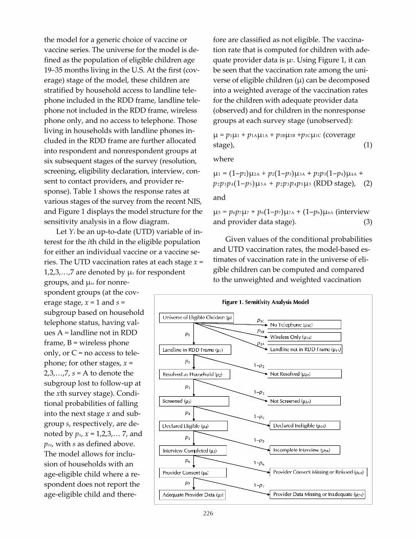
226

the model for a generic choice of vaccine or vaccine series. The universe for the model is de‐fined as the population of eligible children age 19–35 months living in the U.S. At the first (cov‐erage) stage of the model, these children are stratified by household access to landline tele‐phone included in the RDD frame, landline tele‐phone not included in the RDD frame, wireless phone only, and no access to telephone. Those living in households with landline phones in‐cluded in the RDD frame are further allocated into respondent and nonrespondent groups at six subsequent stages of the survey (resolution, screening, eligibility declaration, interview, con‐sent to contact providers, and provider re‐sponse). Table 1 shows the response rates at various stages of the survey from the recent NIS, and Figure 1 displays the model structure for the sensitivity analysis in a flow diagram.  

Let Yi be an up‐to‐date (UTD) variable of in‐terest for the ith child in the eligible population for either an individual vaccine or a vaccine se‐ries. The UTD vaccination rates at each stage x = 1,2,3,…,7 are denoted by μx for respondent groups, and μxs for nonre‐spondent groups (at the cov‐erage stage, x = 1 and s = subgroup based on household telephone status, having val‐ues A = landline not in RDD frame, B = wireless phone only, or C = no access to tele‐phone; for other stages, x = 2,3,…,7, s = A to denote the subgroup lost to follow‐up at the xth survey stage). Condi‐tional probabilities of falling into the next stage x and sub‐group s, respectively, are de‐noted by px, x = 1,2,3,… 7, and pxs, with s as defined above. The model allows for inclu‐sion of households with an age‐eligible child where a re‐spondent does not report the age‐eligible child and there‐

fore are classified as not eligible. The vaccina‐tion rate that is computed for children with ade‐quate provider data is μ7. Using Figure 1, it can be seen that the vaccination rate among the uni‐verse of eligible children (μ) can be decomposed into a weighted average of the vaccination rates for the children with adequate provider data (observed) and for children in the nonresponse groups at each survey stage (unobserved): 

μ = p1μ1 + p1Aμ1A + p1Bμ1B +p1Cμ1C (coverage stage),   (1) 

where 

μ1 = (1–p2)μ2A + p2(1–p3)μ3A + p2p3(1–p4)μ4A + p2p3p4(1–p5)μ5A + p2p3p4p5μ5 (RDD stage),   (2) 

and  

μ5 = p6p7μ7 + p6(1–p7)μ7A + (1–p6)μ6A (interview and provider data stage).   (3)  

Given values of the conditional probabilities and UTD vaccination rates, the model‐based es‐timates of vaccination rate in the universe of eli‐gible children can be computed and compared to the unweighted and weighted vaccination 

227

rate among children with adequate provider data. Since vaccination rates among nonre‐spondent groups are not known, we can postu‐late probability distributions that reflect the uncertainty in their true values. It may be pos‐sible to derive the probability distribution of μ given certain postulated probability distribu‐tions for the vaccination rates in the nonre‐sponse groups. We propose Monte Carlo simulation to sample from the postulated dis‐tributions. Note that we ignore random error introduced by sampling.  

The proportionate distribution of the uni‐verse of eligible children by telephone status, including landline only (p1 + p1A), wireless only (p1B), or no phone access (p1C), will be based on respective proportions of households with age‐eligible children from the recent National Health Interview Survey (NHIS). For example, Table 2 shows the prevalence of having access to landline telephone, access to wireless only 

phone, and no phone access from the 2005 NHIS. The landline population can be further subdi‐vided into those in (p1) and not in (p1A) the RDD sampling frame. We assume here that condi‐tional probabilities are fixed (e.g., observed from the 2005 NIS): p7 = P{adequate provider data | provider consent}; p6 = P{provider consent | completed interview}; and p5 = P{interview completed | screened and declared eligible}.  

Because the observed eligibility rate among screened households is lower than expected (e.g., 3.2% for the NIS in 2005 vs. 4–5% in the U.S.), some eligible households may not declare a child’s eligibility during the screening, or eli‐gible households may be resolved or screened at lower rates than ineligible households. The model will allow for a different vaccination rate for children from eligible households that de‐clare eligibility during the screener compared to those for whom eligibility is not declared. The model includes three conditional probabilities 

Table 2. Prevalence of Children Age 1–3 Years Living in Landline, Wireless Phone Only, & Phoneless Households, by Selected Characteristics, National Health Interview Survey, 2005 HOUSEHOLDS W/O LANDLINE SERVICE CHARACTERISTIC

LANDLINE TELEPHONE SERVICE Wireless only Phoneless Household

All Children (n=4,329) 86.9% 9.7% 3.4% Race/Ethnicity

Hispanic 82.6 12.0 5.4 White, non-Hispanic 89.6 8.0 2.4 Black, non-Hispanic 81.6 14.0 4.4 Multiracial, non-Hispanic 80.9 13.7 5.4 All other, non-Hispanic 95.0 4.0 1.0

Household Size 2 65.5 23.3 11.2 3 84.2 12.1 3.7 4+ 88.8 8.3 2.9

Living Arrangement Rented house 75.2 17.7 7.1 Owned house or being bought 93.9 5.3 0.8 Other living arrangement 76.0 14.1 9.8

Health Insurance Status Uninsured 77.2 16.2 6.6 Insured 87.8 9.2 3.0

Income to Poverty Ratio Income below poverty level <100% 75.4 16.4 8.3 Poverty level 100–199% 80.2 16.8 3.0 Poverty level 200–399% 89.6 9.0 1.4 Poverty level >400% 97.4 2.6 0.0

Residence Urban area 86.2 10.2 3.6 Rural area 89.4 8.2 2.4

228

related to resolution of cases as households, screening, and declaration of eligibility: p2 = P{resolved | eligible}; p3 = P{screened | resolved and eligible}; and p4 = P{declare eligible | re‐solved, screened and eligible}. These three con‐ditional probabilities can be expressed in terms of resolution, screening and residential rates, the estimated population eligibility rate, and the eligibility rates among resolved and screened households: 

p2 = P{R} * P{HH|R} * P{E|R,HH} / P{E|HH} * P{HH}   (4) 

p3 = P{E|R,S,HH} * P{S|R,HH} / P{E|R,HH}   (5) 

p4 = P{dE|R,S,HH} / P{E|R,S,HH}   (6) 

The following quantities can be obtained from the NIS: P{R} = resolution rate, P{HH|R} = residential rate among resolved households, P{S|R,HH} = screener completion rate among resolved households, and P{dE|R,S,HH} = pro‐portion of resolved screened households that declare eligibility. The quantity P{E|HH} is the population eligibility rate among households with landlines sampled from the RDD frame, which can be obtained from the NHIS or other sources. The quantity P{HH} is the proportion of telephone numbers sampled from the RDD frame that represent households, which must be estimated or treated as random with a postu‐lated probability distribution. The remaining two probabilities will be treated as random with postulated probability distributions: P{E|R,HH} = eligibility rate among resolved households and P{E|R,S,HH} = eligibility rate among resolved, screened households. Assum‐ing these two probabilities are both equal to the eligibility rate among households, p3 becomes a function of observed rates, and p4 becomes the ratio of the observed eligibility rate and the population eligibility rate. However, it is possi‐ble that p4 = 1, implying that eligible households resolve or screen at different rates than noneli‐gible households.   

POSTULATING PROBABILITY DISTRIBUTIONS FOR

VACCINATION RATES AMONG UNOBSERVED

GROUPS

An analysis of the NHIS data could be used to obtain possible choices for probability distri‐butions for vaccination rates in wireless‐only (μ1B) and no‐phone‐access (μ1C) households. A logistic regression model predicting UTD vac‐cination status will be fit using NIS data, with candidate covariates that are available in both NIS and NHIS data sets. The fitted model will then be applied to the NHIS landline‐only, wireless‐only, and no‐phone‐access households to simulate vaccination status in each group. The differences between simulated vaccination coverage in wireless only vs. landline only and no phone access vs. landline only will be com‐puted. The resulting distributions of differences in vaccine coverage will be used for the Monte Carlo simulation. In one run of the simulation, a value will be drawn from each of these differ‐ence distributions, and then the model‐based estimate of the vaccination rate among the uni‐verse of eligible children (μ) will be computed (e.g., assuming p1A = 0 and using the current value of μ1 based on previous survey stages, μ = p1μ1 + p1B[μ1 + differenceB] +p1C[μ1 + differenceC]).  

Completed household interview data are available to guide choices for probability distri‐butions for proportions of children with a com‐pleted interview but missing or denied consent to contact providers (μ6A) and with consent to contact provider but provider data are missing or inadequate (μ7A). First, a logistic regression model predicting UTD vaccination status will be fit using children with adequate provider data, including covariates shown to be associ‐ated with vaccination and household‐reported UTD status. The fitted model then will be used to compute vaccination status for children in groups 6A (completed interview but consent to contact providers not obtained) and 7A (completed interview with consent to contact providers but provider data missing or inade‐quate), and vaccination coverage computed for each simulation. The distribution of computed 

229

vaccination coverage estimates will be used in the simulation to draw values for μ6A and μ7A. This approach is similar to the response pro‐pensity method currently used in NIS adjust‐ments for nonresponse at these stages, which assumes data are missing at random within re‐sponse propensity weighting classes. To allow some degree of violation of this assumption, the simulated values for μ6A and μ7A can be multi‐plied by a constant factor. Another approach would be to include telephone‐exchange‐level sociodemographic variables in the logistic re‐gression model, to see if these ecologic variables add predictive value after controlling for indi‐vidual level factors. Or, vaccination status based on shot records could be compared be‐tween children with and without consent or adequate provider data, among the subset for whom parents reported vaccinations from a shot record during the household interview. 

Only telephone‐exchange‐level ecologic variables will be available for the four nonre‐spondent groups without completed interviews (2A = not resolved, 3A = not screened, 4A = de‐clared ineligible, and 5A = incomplete inter‐view). Using children with adequate provider data, a logistic regression model will be fit to predict UTD vaccination status based solely on exchange‐level covariates. This model can then be used to simulate vaccination status among children with incomplete interviews and then to compute vaccination rates. The distribution of vaccination rates would be used in the simula‐tion to draw a value for μ5A. A similar approach can be used to draw values for screened eligible children declared ineligible (μ4A), children in re‐solved households that were unscreened (μ3A), and children in households that were unre‐solved (μ2A). However, the simulation would have to be done on the pooled cases: declared ineligible (actually eligible and ineligible), not screened (eligible and ineligible), and not re‐solved (eligible, ineligible, not household).  

To provide additional information about nonresponse at different stages, level of effort analysis will be conducted, similar to the ap‐

proach described in Skalland et al. (2006) using number of call attempts. This will provide in‐formation about potential bias at resolution, screener, and interview stages. Specifically, es‐timated vaccine coverage among children with adequate provider data will be examined by number of call attempts: until resolution, be‐tween resolution and screener, between screener and interview completion, and be‐tween interview completion without provider consent until provider consent. Bias will be es‐timated as the difference between estimated vaccination rates for low‐ versus high‐burden responders. Similar analysis could be done us‐ing incentive cases, implemented in the NIS in 2006 for cases that were partially through the screener, that dropped out initially during the interview, or that completed the interview without giving consent to contact providers.  

Another potential source of information will be a study of the use of immunization informa‐tion systems (IIS) in two states as sampling frames for the NIS. Briefly, the NIS interview and provider record check procedures will be conducted on random samples of 19–35 month old children selected from each IIS. The vacci‐nation rates as measured by the IIS will be de‐termined for response and nonresponse groups to estimate bias at the screener and subsequent stages. Although the two selected IIS to be stud‐ied have high provider participation, they are unlikely to have 100% complete vaccination his‐tories, and it is possible that completeness of vaccination histories on the IIS may be corre‐lated with likelihood of response at some stages to the NIS survey.  

To assess the overall noncoverage and non‐response bias across RDD survey stages, weighted NIS estimates among households with completed interviews of selected variables available on both NIS and NHIS and associated with vaccine coverage (e.g., health insurance status, income‐to‐poverty ratio, parental report of child’s influenza vaccination) can be com‐pared to similar estimates from the NHIS over‐all and among landline only populations. 

230

SIMULATION PROCEDURE

To allow for the situation where input to the simulation model is in the form of a postulated bias (difference between vaccination rates in re‐sponse vs. nonresponse groups), each run of the simulation will begin at the last stage of the sur‐vey process and work backwards. For example, a vaccination rate value will be drawn first for children with a completed interview but not having adequate provider data (μ7A), and then a vaccination rate value for children with provider consent will be computed as a weighted average of rates for those with and without adequate provider data [μ6 = p7μ7 + (1–p7)μ7A]. Then, a vac‐cination rate value for children with completed interview but without consent (μ6A) will be drawn and combined with the value for μ6 to yield a value for μ5. This process will continue up to the universe of eligible children, with a fi‐nal value for μ computed.  

The simulation will be run 1,000 times, or fewer if stable distributions are generated with fewer runs. For each run, estimates of overall bias will be computed using unweighted esti‐mates (μ7 – μ), as well as estimates of bias at each survey stage (e.g., μ7 – μ7A, μ6 – μ6A, μ5 – μ5A, μ4 – μ4A, μ3 – μ3A, μ2 – μ2A, μ1 – μ1A, μ1 – μ1B, μ1 – μ1C, μ1 – μ). The extent to which the weighted estimate of μ7 is closer to μ than the unweighted estimate also will be examined, and the final es‐timated bias in reported vaccination rates esti‐mated by μ7(weighted) – μ. To assess the influence of nonresponse at different stages, we can widen the uncertainty in vaccination rate dis‐tribution for a given stage, using the “best” model distributions for other stages, and exam‐ine the resulting distribution of bias. Alterna‐tively, we can use the “best” model distribution for a given stage and assume no bias in other stages.   DISCUSSION

SUMMARY

We propose a framework for quantifying systematic error in a RDD survey that targets 

households with young children, identifies the children’s providers, and then surveys these providers to collect validated vaccination histo‐ries. The model includes noncoverage of the RDD frame and explicitly defines nonresponse groups at each stage of the survey process. We propose to conduct a variety of noncoverage and nonresponse bias assessment studies to provide input into the model. The model can be established before any of these studies are completed and re‐run as new information is ob‐tained. Monte Carlo simulation is proposed to quantify the uncertainty in model input pa‐rameters and to allow flexible assumptions about input probability distributions without having to derive joint probability distributions.   

STRENGTHS

A main strength of this approach is to ex‐plicitly define each of the survey stages where systematic error can arise. This can identify stages where relatively little information is available about vaccination rates in nonre‐sponders and which stages are potentially most influential in introducing nonresponse bias. This approach also facilitates planning of stud‐ies to assess nonresponse bias. A variety of ap‐proaches have been proposed to assess nonresponse bias, each with its own limitations. The approach proposed here synthesizes in‐formation from these studies, and translates them into the main quantity of interest, the bias due to noncoverage and nonresponse. Potential uses of the model include identifying influen‐tial survey stages to target for reductions in nonresponse bias, modeling potential effects of specific efforts to improve response rates or re‐duce nonresponse bias (e.g., incentives), identi‐fying survey stages for which additional information is critical in reducing variability in the simulated distribution of bias, aiding in in‐terpretation of response rates and deciding how to report them, evaluating current weighting and adjustment approaches and modeling po‐tential effects of potential improvements, and modeling of potential differential nonresponse 

231

by subgroups (e.g., race/ ethnicity, geographic area).  LIMITATIONS

Like any sensitivity analysis, findings will be determined in part by assumptions that must be made in the model structure and input parameters. In absence of direct estimates of vaccination rates in groups not covered by the sampling frame or who do not respond at vari‐ous stages, findings from the sensitivity analysis cannot be absolutely definitive. In application to the NIS, we have a rich set of data to assess non‐response related to the provider phase of the survey and less information on upstream stages of the RDD component. Particularly, there is lit‐tle information available on eligibility rates among resolved and screened households and the extent to which screened eligible house‐holds fail to declare their eligibility. Even for assessment of bias at the provider phase of the survey, where we have household‐reported in‐formation on factors associated with vaccine coverage, we must make assumptions that non‐response is not related to vaccination coverage after controlling for these factors or postulate departures from these assumptions. The NHIS data can provide valuable information regarding potential noncoverage bias. The NHIS covers both telephone and nontelephone households in the survey. However, this analysis will be lim‐ited by available sample size for households with young children and must be repeated at least annually, given the steady increase in prevalence of wireless‐only households. The NHIS data is itself subject to error from nonre‐sponse and misclassification of household tele‐phone status. Also, without provider‐validated vaccination status available for NHIS respon‐dents, we must rely on proxy measures avail‐able on NHIS or compute vaccination status using a model based on factors associated with coverage. In this paper, we did not incorporate information on geographic stratum in the model nor did we address potential bias in vac‐cination coverage among subgroups (e.g., by 

race/ethnicity). There may be variations in re‐sponse rates at different stages and in eligibility rates by geographic stratum.   NEXT STEPS

It is likely we will refine the model as we de‐velop it for the NIS. Once implemented and re‐vised as more information about potential nonresponse and noncoverage bias become available from proposed studies, its value can be reassessed. It may be that simpler approaches, such as benchmarking to the NHIS or other sur‐veys, will provide adequate assessment of po‐tential bias in future years of the survey. For example, questions on health insurance status were added starting with the 2006 NIS, and we are adding a question on parental report of in‐fluenza vaccination on the NIS starting in 2007, similar to a question currently on the NHIS. It is possible to incorporate measurement error and confounding into the model. For example, our current definition for having adequate provider data allows inclusion of children with multiple providers for whom not all identified providers responded, which likely results in underestima‐tion of vaccination coverage to some extent. The NIS has been expanded to include an immuni‐zation survey of children age 13–17 years using the NIS sampling frame, including a provider record check phase. A similar sensitivity analysis model needs to be developed for this survey. Given rising prevalence of wireless‐only house‐holds and declining response rates to RDD sur‐veys, it is imperative that potential systematic error is quantified rigorously and periodically for RDD surveys. The proposed framework at‐tempts to do this. Even if the sensitivity analysis yields a relatively wide distribution of potential bias, it is better to acknowledge this than to make implicit assumptions about lack of bias when reporting results or simply stating that residual bias of unknown direction and magni‐tude may remain after weighting adjustments.  

232

REFERENCES

Battaglia, M. P., Khare, M., Frankel, M. R., Murray, M. C., Buckley, P., & Peritz, S. (in press). Re‐sponse rates: How have they changed and where are they headed? In J. M. Lepkowski, N. C. Tucker, J. M. Brick, E. D. de Leeuw, L. Japec, P. J. Lavrakas, M. W. Link, & R. L. Sangster (Eds.), Advances in telephone survey methodology. New York: Wiley. 

Blumberg, S. J., Luke, J. V., & Cynamon, M. L. (2006). Telephone coverage and health survey esti‐mates: Evaluating the need for concern about wireless substitution. American Journal of Public Health, 96, 926–931.  

de Leeuw, E., & de Heer, W. (2002). Trends in household survey nonresponse: A longitudinal and international comparison. In R. M. Groves, D. A. Dillman, J. L. Eltinge, & R. Little (Eds.), Survey nonresponse. New York: John Wiley & Sons. 

Ezzati‐Rice, T. M., Frankel, M. R., Hoaglin, D. C., Loft, J. D., Coronado, V. G., & Wright, R. A. (2000). An alternative measure of response rate in random‐digit‐dialing surveys that screen for eligible subpopulations. Journal of Economic and Social Measurement, 26, 99–109. 

Graham, J. D. (2006, January 20). Memorandum for the President’s Management Council. Executive Office of the President, Office of Management and Budget. Retrieved August 1, 2007, from www.whitehouse.gov/omb/inforeg/pmc_survey_guidance_2006.pdf 

Greenland, S. (2005). Multiple‐bias modeling for analysis of observational data. Journal of the Royal Statistical Society A, 168, 267–306. 

Groves, R. M. (2006). Nonresponse rates and nonre‐sponse bias in household surveys. Public Opinion Quarterly, 70, 646–675. 

Groves, R. M., & Couper, M. P. (1998). Nonresponse in household interview surveys. New York: Wiley. 

Hogan, H., & Wolter, K. M. (1988). Measuring accu‐racy in a post‐enumeration survey. Survey Meth‐odology, 14, 99–116. 

Johnson, T. P., Cho, Y. I., Campbell, R. T., & Hol‐brook, A. L. (2006). Using community‐level cor‐relates to evaluate nonresponse effects in a telephone survey. Public Opinion Quarterly, 70, 704–719. 

Lash, T. L. (2007). Heuristic thinking and inference from observational epidemiology. Epidemiology, 18, 67–72. 

Lash, T. L., & Fink, A. K. (2003). Semi‐automated sensitivity analysis to assess systematic errors in observational data. Epidemiology, 14, 451–458. 

Link, M. W., Mokdad, A. H., Kulp, D., & Hyon A. (2006). Has the National Do Not Call Registry helped or hurt state‐level response rates? A time series analysis. Public Opinion Quarterly, 70, 794–809. 

Mulry, M. H., & Spencer, B. D. (1991). Total error in PES estimates of population. Journal of the Ameri‐can Statistical Association, 86, 839–863. 

Phillips, C. V. (2003). Quantifying and reporting un‐certainty from systematic errors. Epidemiology, 14, 459–466. 

Salmon, D. A., Smith, P. J., Navar, A. M., Pan, W. K. Y., Omer, S. B., Singleton, J. A., et al. (2006). Measuring immunization coverage among pre‐school children: Past, present and future oppor‐tunities. Epidemiologic Reviews, 28, 27–40. 

Skalland, B., Wolter, K., Shin, H. C., & Blumberg, S. J. (2006). A nonresponse bias analysis to inform use of incentives in multistage RDD telephone surveys. Paper presented at the 2006 Joint Statistical Meetings, Seattle. 

Smith, P. J., Hoaglin, D. C., Battaglia, M. P., Khare, M., & Barker, L. E. (2005). Statistical methodology of the National Immunization Survey: 1994–2002 (Vital and Health Statistics, Series 2, No. 138). Hyattsville, MD: National Center for Health Sta‐tistics.  

Smith, P. J., Rao, J. N. K., Battaglia, M. P., Ezzati‐Rice, T. M., Daniels, D., & Khare, M. (2001). Compensating for provider nonresponse using re‐sponse propensities to form adjustment cells: The Na‐tional Immunization Survey (Vital and Health Statistics, Series 2, No. 133). Hyattsville, MD: National Center for Health Statistics.  

233

FEATURE PAPER: Accommodating a Changing Panel Design Darryl V. Creel, RTI International

  INTRODUCTION

Panel surveys, in which the same sampling units are surveyed at different points in time, often are subject to a number of unique chal‐lenges. For instance, over time, analytical objec‐tives of the research can change or evolve. In other situations, there can be changes with re‐spect to availability of resources, funding, and data collection cost structure. All such changes can impact the panel survey design and the sampling units that are retained in the panel. Retention of the sampling units is particularly important because of the difficulty associated with recruiting sampling units and the benefits of continuity for variance estimation purposes. An example of changing survey objectives is when the analytical subdomains—e.g., geo‐graphic areas for which accurate estimates are required—expand, shrink, or shift. Conse‐quently, it is possible for precision require‐ments of key survey estimates to increase or decrease. Changes in available resources, which include an increase in the cost of data collection and a reduction in funding, are rather obvious and more frequent. 

In order to address these challenges, we de‐scribe Esbjorn Ohlsson’s (1992, 1995, 1999) work on sample coordination based on the use of per‐manent random numbers that can readily adapt to changes in analytical objectives, resources, and data collection costs while maintaining many of the benefits of a panel survey design that lead to more accurate estimates of change over time. The advantage of this design is that it is easy to understand and implement. Specifi‐cally, while maintaining the probabilistic nature of each selection, this design allows the overlap between the two samples to be large. The flexi‐bility of our proposed method provides a sim‐ple and efficient way to accommodate modifi‐cations to the panel survey design that can oc‐

cur over time. Consequently, data collection ac‐tivities can proceed without any delay or loss of continuity for implementing controlled selection1 or some other method to address the emerging design changes. Additionally, the design intro‐duces no further complications for sampling, weighting, variance estimation, or analysis for individual time periods or trends. That is, we reap the benefits of the design at virtually no cost, and the loss of efficiency due to changes in the panel survey design is small. Finally, we discuss some further research that could possi‐bly extend Ohlsson’s work to account for non‐response. 

This paper will illustrate the design meth‐odology by using an example where sampling units, which are hospitals, are stratified by state, size of hospital, and ownership (i.e., pub‐lic or private). The initial sample has propor‐tional allocation with respect to the states and aims to produce accurate national estimates. The subsequent samples reflect any changes, if any, in the panel survey design. Also, the sub‐sequent samples update the previous sample to account for new sampling units or newly eligi‐ble sampling units added to the population each year. The paper focuses on the implemen‐tation of the design and also discusses the de‐sign with respect to frame development, sampling, weighting, variance estimation, and analysis, including individual time periods and trends.  

1 Controlled selection is “any process of selection in which, while maintaining the assigned probability for each unit, the probabilities of selection for some or all preferred com‐binations of n out of N units are larger than in stratified random sampling (and correspondingly the probabilities of selection for at least some non‐preferred combinations are smaller than in stratified random sampling)” (Goodman & Kish, 1950, p. 351). The most common approach is described in Kish and Scott (1971), which extends the Keyfitz (1951) method.

234

SURVEY DESIGN

The main features of this type of survey de‐sign are 1. It is a panel survey. 2. It incorporates permanent random num‐

bers. 3. It can use stratification, simple random 

sampling, and/or probability proportional to size sampling. 

 

Each of these features is discussed below. The main reason for having a panel survey 

is that it can detect smaller differences between time periods than repeated cross‐sectional sur‐veys can.2 This is due to the fact that the sam‐pling units are their own controls from one time period to the next. That is, the panel survey can measure the changes related to the same sam‐pling units from one time period to the next. In general, multiple measurements on the same sampling unit are positively correlated, and there frequently is a high positive correlation. The panel design takes advantage of this and is able to produce smaller variances when testing differences from one period to the next, which, in turn, allows analysts to detect smaller differ‐ences that may go undetected when repeated cross‐sectional surveys are used. 

Repeated cross‐sectional surveys use the same design from one time period to the next but collect information from independent sam‐ples in each period. Because of this, the inde‐pendent samples contain an additional amount of variability; the more variability in the esti‐mates, the more difficult it is to detect differ‐ences between time periods. The variance of a 

2 Pp. 457–477 in Kish (1965) contain sections 12.4, Correla‐tions from Overlaps in Repeated Surveys, and 12.5, Panel Studies and Designs for Measuring Change. These sections provide detailed explanations of the variance calculations for repeated cross‐sectional, panel, and rotating panel de‐signs. They also document the advantages of panel or ro‐tating panel design with respect to gross change behind a net change between two years. Duncan and Kalton (1987) provide an overview of the ad‐vantages and disadvantages of various designs of surveys across time. 

difference of two means for a panel survey and repeated cross‐sectional surveys will be exam‐ined in the variance estimation section of this paper. 

A permanent random number (PRN) is a unique and independent random number gen‐erated from uniform distribution on the interval (0,1). The PRN is generated for each sampling unit in the population and remains with the sampling unit as long as the sampling unit is on the frame (Ohlsson, 1992, 1995). The PRN al‐lows us to have very large overlap between time periods of the panel survey. 

Stratification partitions the frame into dis‐joint sets of sampling units with independent sampling within strata. It is an equal probabil‐ity selection method within strata. Within a stratum, the sampling can be simple random sampling—i.e., each sampling unit has the same probability of selection—or probability propor‐tional to size (PPS) sampling. 

 FRAME DEVELOPMENT

Frame development consists of the initial frame development and periodic frame updates.  INITIAL FRAME DEVELOPMENT

During the initial frame development, the normal frame development tasks (i.e., creating unique sampling unit identifiers, creating strati‐fication variables, and eligibility determination) occur with the additional task of assigning PRNs to the sampling units on the frame.  PERIODIC FRAME UPDATES

During any periodic update, a new sam‐pling unit may be added to the frame or there may be some type of change related to sam‐pling units already on the frame. A new sam‐pling unit is referred to as a “birth,” and the birth is assigned a PRN. We can check the PRN against the PRNs already on the frame and the other births to ensure it is unique. Conversely, when a sampling unit leaves the frame, referred 

235

to as a “death,” its PRN is deleted with it (Ohls‐son, 1992; 1995). Srinath and Carpenter mention a potential disadvantage to this approach to births: “…the PRNs of births [may not be] equally spaced on the interval [0,1]. This may lead to births being over‐ or underrepresented in the sample due to random chance” (1995, p. 174). To check for this problem, we can monitor the distribution of the PRNs for the births at each periodic frame update and cumulatively. Also, if the number of births is small, this should not be a problem. 

Other types of changes (Struijs & Wille‐boordse, 1995) that may occur to sampling units already on the frame are a change in a particu‐lar characteristic of the sampling unit or a change of structure. Changes of structure in‐clude concentration, deconcentration, and re‐structuring.  SAMPLE ALLOCATION

The initial sample can use any of the stan‐dard procedures to optimally allocate the sam‐ple. In the subsequent samples, whether to reallocate the sample will depend on the com‐plexity and magnitude of the changes to the survey design.  SAMPLE SELECTION

To select a simple random sample of size n sampling units from a population of size N without replacement in a stratum, we use a se‐quential simple random sampling without re‐placement method.  

Method 4 in Fan, Muller, and Rezucha (1962) describes a two‐stage sequential selection method to achieve this. In stage one, a uniform random number on the interval (0,1) is gener‐ated for each sampling unit. Assuming that these uniform random numbers are unique and independent, place the first n sampling units in a “reservoir.” For the remaining N – n sampling units, if a sampling unit’s uniform random number is less than the largest uniform random number in the reservoir, include the sampling 

unit in the reservoir. Otherwise, ignore the sam‐pling unit. For stage two, select the n sampling units in the reservoir with the smallest uniform random numbers. This provides a simple ran‐dom sample without replacement of size n. 

Ohlsson (1992, 1995) references the equal probability sampling JALES technique,3 which permanently associates the uniform random numbers to the sampling units creating PRNs. Using PRNs, Ohlsson (1992, 1995) describes a simpler sequential simple random sampling without replacement method. The sampling units are sorted by the PRNs, and the first n sampling units are selected for the sample. This provides a simple random sample without re‐placement of size n. Ohlsson (1992) provides a formal proof of this in Appendix 1. 

To select a probability proportional to size sample of n sampling units from a population of N without replacement in a stratum, we will use a sequential random sampling technique rec‐ommended by Ohlsson (1999) based on Monte Carlo simulation. The technique is Pareto sam‐pling, which was introduced by Rosen (1997). Pareto sampling is similar to sequential simple random sampling, but instead of sorting on the PRN alone, we sort on a function of the PRN, the measure of size, and the sample size in the stra‐tum. The function for Pareto sampling is 

Xi/(1 – Xi)  ξi =

npi/(1 – npi), 

 

where ξi is the value that will be sorted for the ith sampling unit, Xi is the PRN for the ith sam‐pling unit, n is the sample size in the stratum, and pi is the normed measure of size for the ith sampling unit, where the normed measure of size means that the sum of all of measures of size equals one. After sorting on the ξi, we se‐lect the first n sampling units.  3 “In the SAMU [the coordinated sample system at Statistics Sweden], samples are drawn by the so called JALES tech‐nique, developed at Statistics Sweden in the early 70’s by Johan Atmer and Lars‐Erik Sjöberg (for whom ‘JALES’ is an acronym)” (Ohlsson, 1992, p. 2). “The Swedish SAMU sys‐tem uses sequential srswor with PRNs to coordinate sam‐pling across surveys and over time” (Ohlsson, 1995, p. 155). 

236

WEIGHTING

For stratified simple random sampling, the design weight for a stratum is the inverse of the probability of selection for the sampling units selected into the sample and zero for the sam‐pling units not selected into the sample. That is, the design weight for a stratum is the popula‐tion size of the stratum divided by the sample size of the stratum for the sampling units se‐lected for the sample and zero for the sampling units not selected for the sample. For stratified PPS sampling, the probability of selection is 1/npi, where n is the sample size for the stratum and pi the measure of size for the ith sampling unit, for sampling units selected into the sample and zero for the sampling units not selected into the sample. Any other weighting adjustments—e.g., nonresponse or poststratification—are conducted normally. Therefore, the design does not cause any complications when calculating the design weights or any other weighting ad‐justment.  VARIANCE ESTIMATION

Since we are using stratified sampling, we can easily use the same strata for estimating the variance. The variance is estimated using the standard formulas. As mentioned in the survey design section of the paper, to get an idea of the reduction in the variance estimates for the panel design versus a repeated cross‐sectional design, we show the argument with the vari‐ance for the difference of two means. 

Let t1 be the mean for time period one and t2 be the mean for time period two. Using simpli‐fying assumptions that the variances for the means are equal for the two time periods, 

1

2tS =

2

2tS = 2S , and that the sample sizes are equal 

for the two time periods, nt1 = nt2 = n, the vari‐ance for the difference of the two means for a repeated cross‐sectional design is  

var(t2 – t1) = 22 .n S  

Finally, let the correlation between the outcome variable at two time periods be ρt1t2 and the amount of overlap between the two samples by λ. The variance for the difference of two means for the panel design is  

var(t2 – t1) = 2n S2(1 – λρ t1t2). 

Comparing the variance for the difference of two means for the repeated cross‐sectional de‐sign and the variance for the difference of two means for the panel design, we see that the variance for the difference of two means for the panel design is smaller by a factor of (1 – λρt1t2). That is, the variance is reduced by the product of the amount of overlap between the two sam‐ples and the correlation between the outcome variable at two time periods.  ANALYSIS

There are two possible types of analysis. The first type is the independent analysis of the individual time periods, and the second type is the analysis of trends. The two most common types of trend analysis are comparing a time period with the initial, or base, time period and comparing two consecutive time periods.  INDIVIDUAL TIME PERIODS

For the individual time periods, any soft‐ware designed to analyze survey data, i.e., software that can account for the survey design and differential weighting, such as SUDAAN, can be used.   TREND ANALYSIS

For the trend analysis, if the variable names on the two data sets have the same names, ap‐pend—i.e., stack—one of the data sets to the other. Then any software designed to analyze survey data can be used. Each sampling unit will be considered a cluster for which there are two observations, one for each year.  

237

EXAMPLE

Now that we have the basic idea, let us work through an example to solidify our un‐derstanding of the sampling and weighting. Suppose there is a proposed budget cut in the future, and we want to be prepared to cut back data collection to adhere to the proposed budget cut, if necessary. The example is a strati‐fied sequential simple random sampling without replacement design with a decrease in sample size from the initial sample to the future sample and can be extended easily to Pareto sampling. 

For simplicity, assume we have three strata, each with a population of 20 sampling units; we have selected the initial sample using stratified simple random sampling without replacement using the sample allocation for sample one in Table 1; and we are in the data collection phase. During the data collection phase, an unantici‐pated challenge arises. The data collection chal‐lenge could be a lack of available resources to collect data from all of the sampling units se‐lected into the sample, a reduction in funding, or 

a change in the data collection cost structure where the cost for data collection per sampling unit is higher than expected. To adapt to the data collection challenge, we decide to implement the future sample designed for the proposed budget cut. The new sample size is smaller by one‐third. We calculated the sample allocation for the fu‐ture sample in Table 1. Table 1 contains the stra‐tum, the population size, the initial sample allocation, and the future sample allocation. 

For the initial sample, using the PRNs and the sequential selection method described in the sample selection section of the paper for each stratum, Table 2 shows the sampling units selected. Concisely, we generated a uni‐form random number on the interval (0,1) for 

Table 1. Sample Allocation

Stratum Population Size Initial Sample

Allocation Future Sample

Allocation 1 20 13 9 2 20 9 6 3 20 8 5

Total 60 30 20

Table 2. Selected Sampling Units for the Initial Sample & the Future Sample STRATUM 1 STRATUM 2 STRATUM 3

ID PRN Initial

Sample Future Sample ID PRN

Initial Sample

Future Sample ID PRN

Initial Sample

Future Sample

17 0.124 1 1 8 0.053 1 1 3 0.006 1 1 4 0.156 1 1 11 0.096 1 1 11 0.021 1 1 8 0.182 1 1 1 0.223 1 1 4 0.040 1 1

15 0.189 1 1 18 0.253 1 1 16 0.140 1 1 10 0.341 1 1 10 0.282 1 1 15 0.447 1 1 1 0.350 1 1 17 0.461 1 1 20 0.578 1 0

18 0.416 1 1 14 0.463 1 0 14 0.601 1 0 13 0.429 1 1 3 0.492 1 0 6 0.602 1 0 7 0.430 1 1 9 0.497 1 0 7 0.608 0 0 6 0.480 1 0 20 0.506 0 0 17 0.711 0 0 3 0.491 1 0 7 0.602 0 0 5 0.714 0 0

19 0.516 1 0 19 0.701 0 0 8 0.723 0 0 11 0.600 1 0 4 0.703 0 0 13 0.802 0 0 12 0.675 0 0 2 0.805 0 0 2 0.844 0 0 2 0.684 0 0 6 0.877 0 0 1 0.846 0 0

20 0.702 0 0 12 0.910 0 0 10 0.875 0 0 16 0.706 0 0 13 0.935 0 0 9 0.943 0 0 9 0.775 0 0 5 0.938 0 0 19 0.962 0 0

14 0.779 0 0 16 0.939 0 0 18 0.978 0 0 5 0.887 0 0 15 0.978 0 0 12 0.986 0 0

238

each sampling unit, sorted the sampling units by the PRN, and selected the first nh sampling units in stratum h, where nh is given in Table 1. Table 2 contains the stratum, the ID of the sam‐pling unit, the PRN, and the indicator variable for selection into the initial sample. 

To reduce the sample size by one‐third to adapt to our data collection challenge, we use the same sequential sample selection method used to select the sampling units in the initial sample and the future sample. The only differ‐ence is the change in the number of sampling units selected in stratum h, nh. Table 2 also con‐tains the indicator variable for selection into the future sample. The bolded ones, 1, for the indi‐cator variable for selection into the initial sam‐ple, are the sampling units that are dropped from data collection. For comparison, a simple random sample would contain the italicized sampling units in the future sample column. Note that the simple random sample does not have nearly as much overlap as the sequential simple random sample. This illustrates the con‐siderable overlap provided by the sequential simple random sample methodology as com‐pared to the simple random sample methodol‐ogy.  

Because we have two different sample sizes in each stratum, we need to have two different weights for each stratum: the initial sample de‐sign weight and the future sample design weight. The design weights by stratum for the two samples are shown in Table 3. In this ex‐ample, we have a reduction in sample size from the initial sample to the future sample. Conse‐quently, the design weights by stratum in the 

initial sample are less than the design weight by stratum in the future sample. In either case, the product of the stratum design weight and stra‐tum sample size is equal to the stratum popula‐tion size. 

 CONCLUSION

The events described in this paper demon‐strate the need to be prepared to adjust the panel survey design to meet some change, either planned or unplanned, in the requirements for the panel survey design. The design, which uses permanent random numbers in conjunction with stratified random sampling, is a relatively easy, flexible approach to implement these changes. 

The flexibility of the design can be extended in two ways: allowing the stratification scheme to change and calculating sample size require‐ments at each time period. First, allowing the stratification scheme to change would allow for the incorporation of totally different strata. For example, if the current stratification scheme is based on state, perhaps the incorporation of Core‐Based Statistical Areas (CBSAs) could be added to produce estimates at this level to meet new analytic objectives. Second, calculating sample size requirements at each time period would allow for better allocation of the sample. For example, using information about the size of the variance in strata could assist in produc‐ing optimal sample sizes. Finally, a combina‐tion of changing analytic objectives (e.g., adding CBSAs) and an accompanying increase in funding could be addressed and seamlessly incorporated into the next data collection pe‐riod at virtually no additional cost while main‐taining a very large overlap between the two samples. 

One area for further research extends cur‐rent work to account for which sampling units respond. Ohlsson’s (1992, 1995, 1999) and Rosen’s (1997) work provides significant over‐lap between samples but does not account for whether the sampling units responded. Retain‐ing nonresponding hospitals from the initial sample and dropping responding hospitals 

Table 3. Design Weights for Sample 1 & Sample 2

Stratum Popu

lati

on

Size

Sam

ple

1 A

lloca

tion

Sam

ple

2 A

lloca

tion

Sam

ple

1 D

esig

n W

eigh

t

Sam

ple

2 D

esig

n W

eigh

t

1 20 13 9 1.538 2.222 2 20 9 6 2.222 3.333 3 20 8 5 2.500 4.000 Total 60 30 20

239

would be extremely inefficient. We would like to retain as many of the responding sampling units as possible, particularly if these responding units are extremely important for any reason (e.g., analytic objectives). We are attempting to identify a function that incorporates the re‐sponse propensity, measure of importance, or level of recruitment effort and retains these re‐sponding hospitals in a probabilistic manner. One other aspect we are considering in this re‐search is the effect of the specific hospitals re‐tained on the mean square error of the estimates from the survey data.  REFERENCES

Duncan, G., & Kalton, G. (1987). Issues of design and analysis of surveys across time. International Sta‐tistical Review, 55, 97–117. 

Fan, C. T., Muller, M. E., & Rezucha, I. (1962). De‐velopment of sampling plans by using sequen‐tial (item by item) selection techniques and digital computers. Journal of the American Statisti‐cal Association, 57, 387–402. 

Goodman, R., & Kish, L. (1950). Controlled selec‐tion—A technique in probability sampling. Jour‐nal of the American Statistical Association, 45, 350–372. 

Kish, L. (1965). Survey sampling. New York: John Wiley & Sons. 

Kish, L., & Scott, A. (1971). Retaining units after changing strata and probabilities. Journal of the American Statistical Association, 66, 461–470. 

Keyfitz, N. (1951). Sampling with probabilities pro‐portional to size: Adjustment for changes in the 

probabilities. Journal of the American Statistical Association, 46(235), 105–109. 

Ohlsson, E. (1992). SAMU: The system for co‐ordination of samples from the Business Register at Statistics Sweden—A methodological description (R&D Report 1992:18). Stockholm: Statistics Sweden. 

Ohlsson, E. (1995). Coordination of samples using permanent random numbers. In B. G. Cox, D. A. Binder, B. N. Chinnappa, A. Christianson, M. J. Colledge, & P. S. Kott (Eds.), Business survey methods (pp. 153–169). New York: John Wiley & Sons. 

Ohlsson, E. (1999). Comparison of PRN [Permanent Random Number] techniques for small size PPS sample coordination (Research Report No. 210). Stockholm, Sweden: Stockholm University, In‐stitute of Actuarial Mathematics and Mathe‐matical Statistics. 

Rosen, B. (1997). On sampling with probability pro‐portional to size. Journal of Statistical Planning and Inference, 62, 159–191. 

Srinath, K. P., & Carpenter, R. (1995). Sampling methods for repeated surveys. In B. G. Cox, D. A. Binder, B. N. Chinnappa, A. Christianson, M. J. Colledge, & P. S. Kott (Eds.), Business survey methods (pp. 171–183). New York: John Wiley & Sons. 

Struijs, P., & Willeboordse, A. (1995). Changes in populations of statistical units. In B. G. Cox, D. A. Binder, B. N. Chinnappa, A. Christianson, M. J. Colledge, & P. S. Kott (Eds.), Business survey methods (pp. 65–84). New York: John Wiley & Sons. 

 

241

FEATURE PAPER: Survey Mode Choices: Data Quality and Costs J. Michael Brick and Graham Kalton, Westat

 INTRODUCTION

A key decision to be made early in planning a survey is the mode or modes of data collec‐tion to be used. This paper discusses the factors entering into this choice, with a focus on health surveys of persons and households (rather than establishments). In selecting a primary data col‐lection mode, researchers generally must choose between face‐to‐face (f‐to‐f) interview‐ing, telephone interviewing, mail question‐naires, and Web‐based data collection. In recent years, mixed‐mode surveys have become in‐creasingly attractive as a way to address the limitations of any single mode. Also, with face‐to‐face and telephone modes, there is a further choice to be made between interviewer‐ and computer‐administered questions. 

The choice of mode depends on costs and data quality considerations, and often trade‐offs between the two. In some cases, the choice is made with little debate, but in others, it is less straightforward. In all cases, however, a com‐plex combination of factors must be taken into account in making an informed choice. Costs and quality both have several dimensions. For example, costs associated with a given mode include not only data collection costs but also sampling and processing costs. Quality in‐cludes both data accuracy and timeliness, with accuracy depending on the errors introduced through the measurement process, sampling er‐ror, noncoverage, and nonresponse.  

MODE ALTERNATIVES

FACE-TO-FACE

In the f‐to‐f mode, an interviewer typically contacts the sampled unit and conducts the in‐terview or data collection. Having an inter‐viewer at the door has some significant advantages that are difficult to emulate com‐

pletely in other modes. An interviewer’s physi‐cal presence often results in higher response rates and provides the opportunity to imple‐ment other activities, such as making observa‐tions, collecting specimens (e.g., paint chips, biomarkers), reviewing records (e.g., immuni‐zation cards, prescriptions), helping the re‐spondent understand the data collection requirements, and showing visual aids. Also, incentives can be delivered directly to sampled persons, providing a proximate stimulus to in‐crease response. Finally, f‐to‐f interviewing has a distinct advantage over other modes when the interview is very long (e.g., more than an hour).  

Paper‐and‐pencil (PAPI) methods were used routinely in f‐to‐f interviews until the 1990s, after which computer‐assisted personal interviewing (CAPI) became the main method, especially for large health surveys. Computer administration has substantial benefits over PAPI in terms of data quality, complex navigation of the survey items, timeliness in processing, and availability of paradata (see Couper & Nicholls, 1998, for more on the benefits of computerized methods). Computer administration is now fairly standard in all modes, with the exception of mail surveys. PAPI methods are generally used with the f‐to‐f mode only for smaller or specialized surveys, which are outside the main scope of this review.  

A major reason for introducing computer‐assisted self‐administered interviewing (CASI) methods in f‐to‐f surveys was to avoid the po‐tentially biasing effects of having interviewers ask the questions and record the answers to sensitive items or topics with potentially high social desirability effects. A variant of this method, audio computer‐assisted self‐administered interviewing (ACASI), has the additional benefit of reducing dependence on the literacy of the respondents by presenting the questions over headphones.  

242

The most serious disadvantages of the f‐to‐f mode are the cost of data collection and the time required to field and process a major sur‐vey. Some activities are more extensive and time‐consuming than in other modes, including listing and sampling. The use of the U.S. Postal Service (USPS) Delivery Sequence File (DSF) as a sampling frame of residential addresses for the f‐to‐f mode would result in a reduction in the time (and costs) associated with some of these procedures. However, many questions about the DSF coverage rate are yet to be re‐searched fully, including its coverage for sub‐groups such as rural areas, multiple dwelling units, and rapidly growing areas.  TELEPHONE

Like the f‐to‐f mode, the telephone mode of‐fers the advantages associated with having in‐terviewers contact sampled units and conduct interviews. An additional advantage of this mode is the ability to monitor and assess the performance of the interview process directly during data collection. Technological advances in telephony make this monitoring possible even with decentralized telephone administra‐tion. Another potential advantage of the tele‐phone mode is its suitability for addressing contact and interview problems with non‐English‐speaking respondents. If the instru‐ment is translated into multiple languages, then hiring and training interviewers with the ap‐propriate language skills is feasible with tele‐phone surveys. F‐to‐f and other modes have greater obstacles in dealing with non‐English‐speaking persons. A distinctive feature of the telephone mode is the availability of a relatively comprehensive and inexpensive sampling frame of households based on phone numbers. 

Computer‐assisted methods were devel‐oped and first implemented for the telephone mode, specifically computer‐assisted telephone interviewing (CATI). Almost all but the small‐est surveys currently conducted by phone use CATI. A variant of this mode uses interactive voice response (IVR) technology. The main at‐

traction of IVR is that it eliminates interviewers from the process, providing cost advantages and potentially improving the quality of responses to sensitive items. IVR can be used within a tele‐phone interview to collect responses to sensitive items and then return the respondent to the in‐terviewer. However, the use of IVR as the sole mode is unsuitable for most health surveys of the general population because its impersonal nature results in extremely low response rates. 

The main disadvantages of the telephone mode are low response rates, especially in ran‐dom‐digit‐dialing (RDD) surveys, and reliance on aural communication. Other disadvantages include inability to collect physical specimens and coverage problems in the RDD frame for landline telephones, primarily due to the in‐creasing number of households that are relying only on cell phones. The effect on data quality of the use of IVR to collect responses on sensi‐tive topics has not yet been tested sufficiently. Providing incentives with telephone surveys lacks the immediacy possible with f‐to‐f sur‐veys and addresses for advance mailings.    MAIL

Data collection costs are low with the mail mode because the questionnaire is self‐administered. This mode also avoids possible interviewer effects. Mail data collection allows respondents to control the pace of response, enabling them to consult records or obtain data from another source if necessary. The visual presentation also gives respondents the oppor‐tunity to study the full set of response alterna‐tives before answering and to view visual aids designed to assist comprehension. While mail surveys are still largely based on list frames, the feasibility of using the mail mode for the gen‐eral household population has been enhanced by the availability of the DSF (however, see the issues discussed above regarding use of the DSF for f‐to‐f surveys). 

The main disadvantages of this mode are consequences of the absence of an interviewer. Without an interviewer, methods for sampling 

243

a person within a household and persuading that person to respond are limited, and re‐sponse rates may suffer. Dillman (2007) de‐scribes procedures in which multiple mailings are used to increase response rates, but such approaches may adversely affect the survey’s timeliness. Also, it is not possible to control who completes the questionnaire, which is a particular problem when responses are re‐quired from a specified, perhaps sampled, household member (Scott, 1961). The question‐naire must be simple enough for respondents to be able to navigate it, and its content must be suitable if people with low literacy levels are surveyed. Question ordering techniques cannot be used with the mail mode in the way they can be used with other modes because respondents can read all of the questions before starting to complete a mail questionnaire.   WEB

Because Web surveys are self‐administered, like mail questionnaires, Web‐based data collec‐tion has low costs and eliminates interviewer effects. While the Web shares many of the bene‐fits of the mail mode, it also has the advantages associated with computerized interviews, such as controlling complex skip patterns, making multimedia presentations possible, and allow‐ing direct data entry. Another advantage of this mode is its timeliness.   The main disadvantages of this mode are the limited number of people with ready access to the Web, the absence of a sampling frame for the general population, and very low response rates. As with mail, it is difficult to control who actually completes a Web questionnaire. These serious disadvantages have thus far ruled out the use of the Web as the sole mode for health surveys of the general population.   MIXED MODES

By using two or more modes for data collec‐tion, survey researchers aim to take advantage of the various strengths of different modes in 

the same survey. One approach is to use the lowest cost mode that meets the survey re‐quirements in the first stages of the survey, with more expensive modes used to deal with nonrespondents or those who could not be con‐tacted by the other modes (as, for example, is done in the American Community Survey). Panel surveys also frequently use multiple modes, with f‐to‐f methods used in the initial wave and the less expensive mail, telephone, or Web modes used to the extent possible in sub‐sequent waves. 

In mixed‐mode surveys, the potential for differential mode effects is a major concern—that is, responses to the same items may differ across modes. These effects may come about, in part, because of differences in the preferred de‐signs of data collection instruments for the dif‐ferent modes. A unimode design that does not utilize the optimal features of the different modes has been suggested as a way to avoid this component of mode effects (see the appen‐dix in Dillman, 2007). Evaluating mode effects is generally very difficult if the characteristics of sample persons differ across modes. This is of‐ten the case because the mode is “self‐selected” when the person has not responded to earlier modes or when the information needed to in‐terview the person (e.g., telephone number) by other modes is not available.  

Based on a review of the literature on mode effects and mixed‐mode designs, de Leeuw (1992, 2005) concluded that unambigu‐ous, factual items generally have negligible mode effects, but that sensitive items and those involving social desirability often are re‐ported differently in self‐ and interviewer‐adminis‐tered data collections. Mode effects typically result from the mixing of interviewer‐mediated and self‐administered modes or aural and visual modes. Mode effects are a major concern for panel surveys because estimates of change, a key analytic objective of such surveys, may be confounded with the effects of mixing modes across waves (Dillman & Christian, 2005).  

244

COST & ERROR PROPERTIES

COST

It is extremely difficult to compare data col‐lection costs associated with different modes in a meaningful way. Groves (1989) discusses the difficulties and cites cost ratios for f‐to‐f to tele‐phone surveys ranging from 1:1 to over 4:1 for the time at which he was writing. Even the 4:1 ratio is probably too low now, given changes in telephone data collection costs in the past two decades. One reason that direct comparisons are difficult is that the measurement process varies greatly by mode. Replicating the survey in another mode might not even be feasible. Furthermore, survey content often is tailored to utilize features of the chosen mode, and that content might not have been included with a different mode. For example, respondents might be asked to consult records on visits to medical providers in an f‐to‐f interview because it can be done easily and adds value, even if the record check is not essential to the goals of the survey. Similarly, respondents may be asked to consult records in self‐administered modes. However, such requests are generally not made in telephone surveys because of the potential nonresponse and cost consequences. 

The following are some general observa‐tions for relatively large household surveys:  • F‐to‐f is the most expensive mode, with data 

collection costs perhaps 5–10 times those of an equivalent telephone survey with the same number of respondents. 

• Telephone is the second most expensive mode, with costs between 2–5 times higher than those of a mail survey with the same number of respondents. 

• Mail is more expensive than the Web mode because of its higher processing costs, with the relative cost of mail to Web data collec‐tions rising as the number of respondents increases. 

• Mixed‐mode survey data collection costs typically include not only a weighted aver‐age of the data collection costs of each mode 

but also development costs (fixed costs) as‐sociated with each mode (which drive total costs higher).  

In the f‐to‐f mode, the variable costs of field work are substantial and very different from the variable costs in other modes. For example, travel costs are not a component of any other mode. In f‐to‐f surveys, travel costs for training and for data collection are generally high. For health surveys that cover only a limited geo‐graphic area, these costs are much lower, thus making f‐to‐f surveys more competitive with telephone surveys from the cost perspective.  

Although the telephone mode has many of the same sources of fixed costs as the f‐to‐f mode, the telephone mode fixed costs tend to be substantially lower. Variable costs are also substantially lower for telephone surveys than f‐to‐f surveys because interviewers have higher workloads, and there are usually no travel costs for training or data collection.  

In contrast to the interviewer‐administered modes, fixed costs account for a large propor‐tion of the total cost for the mail and Web modes, even though these costs are substan‐tially less than for the f‐to‐f and telephone modes. Mail surveys incur variable costs be‐cause of postal fees and processing of com‐pleted instruments. With the Web, most of the costs are fixed costs associated with the devel‐opment of the Web application. Since variable costs are limited to any review and editing of the responses, the sample size is often not a concern with Web surveys. However, as noted earlier, there are other concerns that make the Web unacceptable as the only mode.   Mixed‐mode surveys generally have higher fixed costs than might be expected, especially when the same computerized application can‐not be used for all the modes. Most of these costs are the fixed costs associated with mount‐ing the survey in the different modes. Also add‐ing to the fixed costs for mixed‐mode surveys are the special efforts that are needed to deal 

245

with features of the survey that otherwise might lead to mode differences.  SAMPLING ERROR

  Sampling error and variable costs are highly correlated, but the fixed costs component makes the relationship of sampling error with total costs very nonlinear for some modes. Variable costs are also more closely related to sample size than to sampling error. Sampling error depends on the sample design as well as the sample size, and sample design may differ by mode. For example, most f‐to‐f surveys use cluster samples for efficiency, but clustering tends to increase sampling errors. Thus, com‐parisons of costs by mode should be based on equal effective sample sizes (the sample sizes divided by the design effects) rather than equal sample sizes. However, even this relationship is complex because the design effects for different survey estimates differ, thus producing differ‐ent effective sample sizes for the comparisons.   In assessing sampling error requirements and mode choices, some important considera‐tions are level of geographic detail needed (na‐tional, state, local), level of demographic or other domain detail needed, and the screening ratio (number of households screened to reach one eligible). The precision level requirements for the domain estimates or estimates of a rare population may have an enormous effect on the choice of the mode.   When a survey requires precise estimates, especially at smaller geographic levels and for domains or subgroups, then the expensive modes (such as f‐to‐f and, to a lesser extent, telephone) become less feasible. Although re‐search on the use of the less expensive modes is underway, mail and Web surveys are not yet commonplace for most large‐scale government health surveys. Other alternatives that may be considered include the following: • Mixed modes—using the least expensive 

modes for screening and the more expen‐sive modes for interviewing; 

• Two‐phase samples—using less expensive modes to collect data on a large sample, with a second‐phase sample to obtain more detailed data for a subsample; and 

• Small area estimation—using direct esti‐mates for large geographic areas or domains and indirect (model‐based) estimates for smaller domains. 

NONCOVERAGE ERROR

  Coverage is more a function of the frame than the mode, but clearly the two are highly related. The high coverage of the population af‐forded by area probability samples with the f‐to‐f mode is one of its primary advantages. The coverage of the RDD frame was good through the 1990s, with the exception of very low‐income households. Beginning earlier this dec‐ade, the percentage of households without a regular landline telephone began to increase, and by 2006, nearly 10% of adults lived in cell‐phones‐only households (Blumberg & Luke, 2007). Restricting a survey to households with landlines leads to a sizeable undercoverage. Ef‐forts to sample cell phone numbers have begun, but more research is needed to evaluate their effectiveness.   Mail surveys traditionally have required special lists to cover the household population, and in this case the coverage rate depends on the quality of the specific list. The coverage properties of a list are related to its complete‐ness and accuracy for the target population. Most lists have serious limitations for use as sampling frames. Lists obtained from adminis‐trative sources often are inaccurate and out of date. Another common problem is accessing the list, and new restrictions on the use of the Cen‐ters for Medicare and Medicaid Services (CMS) file of Medicare beneficiaries is a good example. The CMS no longer releases names and ad‐dresses to researchers to directly contact benefi‐ciaries.    Although reasonable frames of the popula‐tion exist for f‐to‐f and telephone surveys, there is no equivalent available for mail surveys. The 

246

USPS DSF mentioned earlier may provide a na‐tional frame for mail surveys if further research indicates it has an acceptable coverage rate. Even if its coverage rate is acceptable, the abil‐ity to randomly sample a person within a household and have the sampled person com‐plete the questionnaire is a thorny problem that diminishes the utility of that frame.   As noted above, the coverage of the general population for Web surveys is poor, making the Web unattractive for all but special population surveys at the current time. Although access to the Web in either the person’s home or at work has increased greatly in the past 15 years, it seems to have reached a plateau, with more than 30% of the population still uncovered (Pew Internet and American Life Project, 2006).    Even those people who have access to the Web cannot generally be sampled directly for Web surveys because there is no sampling frame for this population. An approach that has been used to deal with the lack of a Web frame is to sample using another frame/mode (e.g., by telephone) and enlist the sampled members to participate in a panel of Web surveys. If the sampled persons do not have Web access, then it must be provided to them or they remain un‐covered. This approach is still being evaluated; however, it incurs coverage loss depending on the frame used to sample the households and errors from other sources, such as nonresponse (Huggins, Dennis, & Seryakova, 2002; Saris, 1998).   On its own, the Web mode is mainly used to survey specialized populations, such as college students. The Web mode also has been used for surveys of establishments such as medical pro‐viders rather than for household populations.  NONRESPONSE ERROR

  Response rates vary substantially by the mode of contact and data collection. The typical pattern is that f‐to‐f surveys have the highest response rates, followed in order by telephone, mail, and Web surveys. The presence of inter‐viewers is critical to the higher rates, especially 

in the f‐to‐f mode. In the f‐to‐f mode, other methods of increasing response, such as offer‐ing incentives, are easier to administer than in even the phone mode, where promised incen‐tives have not been found to be very effective.   Other factors related to both the use of an interviewer and response rates may be impor‐tant for some surveys. An interviewer can pre‐sent information on the confidentiality of the data supplied by the respondent, respond to re‐spondent queries about confidentiality, and convey the credibility of the sponsor in ways not possible in self‐administered modes. An in‐terviewer is also useful if release forms must be signed before interviews can be conducted (e.g., parent permissions for adolescents to be inter‐viewed). All of these factors tend to benefit the interviewer‐administered modes.   Dillman (2007) argues that mail surveys can overcome some of these obstacles and achieve better response rates if the surveys and the ma‐terials accompanying them are well‐designed. He describes several experiments, mainly for special populations or subgroups, that demon‐strate that good response rates can be achieved by mail. The experiments of Link and Mokdad (2006) add some support to this idea for a more general household population. However, a limitation in Link and Mokdad’s most encour‐aging finding is that it compares response rates from mail surveys of nonrandomly sampled adults to response rates from telephone surveys of randomly sampled adults. More comparable evidence for the general population is needed.   Web surveys have fared poorly in terms of response rates in the few surveys that have used a probability sample from which response rates could be computed. Dillman (2007) sug‐gests that while careful design may improve surveys on the Web, innovative approaches will be necessary to improve response rates.   Thus far, we have considered response rates but not nonresponse bias. This is largely because response rates are much easier to measure than nonresponse bias. Response rates often have been treated as surrogates for nonresponse bias, 

247

but the relationship between the two may be weak (Groves, 2006). For some estimates, fac‐tors such as sponsorship, survey topic, and ac‐cessibility for contact may be more predictive of nonresponse bias than the overall response rate. These factors may or may not be related to mode. The findings of Link and Mokdad (2006) suggest there is greater SES nonresponse bias in general population mail surveys than in phone surveys with comparable response rates. In the absence of a body of evidence, we suspect that most researchers would rank nonresponse bias as lowest in f‐to‐f surveys, followed by the tele‐phone, mail, and Web modes. This ranking matches the response rate rankings by mode stated earlier, even though response rates may be poor predictors of bias.    The nonresponse bias in a survey’s esti‐mates may be reduced by weighting adjust‐ments. However, the effectiveness of these adjustments in reducing bias is also not well‐documented. If nonresponse is correlated with factors such as income, then weighting adjust‐ments in f‐to‐f surveys may have greater poten‐tial to reduce nonresponse bias because features of the area and interviewer observations of the sampled unit can be linked to the sampled units easily. RDD surveys can obtain only aggregate exchange/ZIP code‐level data for the adjust‐ments, and they may be incorrect due to match‐ing problems. In practice the effectiveness of nonresponse weighting adjustments is rarely considered in choosing a mode.   MEASUREMENT ERROR

  Across a wide range of mode research, the largest and most consistent mode effect that has been observed is what de Leeuw (1992) calls the interviewer effect. Her literature review found that respondents in interviewer‐administered surveys give more socially desirable responses than respondents in self‐administered surveys. Most of the literature has compared inter‐viewer‐administered f‐to‐f or telephone surveys to self‐administered mail surveys, with the ef‐fect having been traditionally interpreted as a 

mode effect. However, with the effect also oc‐curring with the use of CASI in f‐to‐f surveys, it is now more appropriately associated with the interviewer than the mode.    Aquilino (1994) conducted an experiment to separate the mode effect from the interviewer effect in a drug and alcohol use survey. He found slightly lower reported usage by phone than f‐to‐f when both were interviewer admin‐istered. However, much larger differences were found between self‐ and interviewer‐adminis‐tered f‐to‐f interviews. Tourangeau, Rips, and Rasinski (2000) reviewed other experiments that show inconsistent results on the difference between modes when the interviewer effect is held constant. In summary, measurement errors in surveys with sensitive topics may be sub‐stantial unless the items are self‐administered; CASI, ACASI, or IVR may be necessary to con‐trol measurement errors for f‐to‐f and telephone surveys that include sensitive topics.   While interviewer administration can be problematic in surveys about sensitive topics unless the proper precautions are taken, not having an f‐to‐f interviewer may make accurate measurements very difficult in other circum‐stances. For example, physical measurements of height and weight are much more accurate than respondent self‐reports. Because interviewers are not present in person, the telephone, mail, and Web modes are not well‐suited for surveys requiring physical measurements.   The other major source of mode differences is related to the method of question presenta‐tion: visual (ACASI, mail, Web) vs. aural (CAPI, phone). Redline and Dillman (2002) show that visual design and layout can greatly affect re‐sponses. Tourangeau et al. (2000) discuss how acquiescence, primacy, and recency differences might be related to the visual or aural presenta‐tion method. Because of its power, visual presen‐tation has the potential to reduce measurement errors by focusing respondents appropriately. For example, respondents may more easily be able to choose one or more items from a long list when the information is presented visually. On 

248

the other hand, poorly designed layouts may have the opposite effect and increase measure‐ment errors. We know of no meaningful rank‐ings of measurement errors by presentation mode.  CONCLUDING REMARKS

  Many factors are considered in deciding which mode or modes are most appropriate for a survey. Every choice involves balancing ad‐vantages and disadvantages associated with the modes. In most national surveys of the house‐hold population, the main alternatives are still the f‐to‐f and telephone modes. There are sev‐eral important advantages of the f‐to‐f mode, especially in health surveys that require physi‐cal measurements, lengthy interviews, or the establishment of a relationship that will support later data collection, such as in longitudinal surveys. On the other hand, the f‐to‐f mode is much more expensive than the other modes.    If the funds for conducting the survey are limited or direct estimates for small subgroups or geographic domains are required, then f‐to‐f interviewing may have to be ruled out. A tele‐phone survey may be the only viable option. Mail surveys are becoming more attractive as response rates and coverage rates fall in tele‐phone surveys. A new round of research is needed to evaluate samples from the USPS DSF with respect to the many nonresponse, noncov‐erage, and control problems discussed earlier.    While the Web is not generally acceptable as the single mode in a survey, it is a prominent option that may be considered in surveys using mixed modes. Whether it is a cost‐effective op‐tion depends on the extent to which respon‐dents use it. Mixed‐mode surveys can be designed to utilize the strengths of the various modes, but mode effects may be a serious prob‐lem and costs may be higher than budgets in some cases.    In the design stage, costs and sampling er‐rors are important considerations that are easily estimated based on extensive past experience. 

Nonresponse and noncoverage are other impor‐tant considerations affecting the mode choice. However, it is disconcerting when these rates are the main consideration. The focus on rates rather than biases may be due to our inability to measure or predict nonsampling errors quanti‐tatively. Decisions on mode choice and other survey design features would be improved if acceptable ways could be found to assess qual‐ity in terms of errors rather than operational features such as response rates. Such quality measures would also help analysts to compare the quality associated with surveys having dif‐ferent sample sizes, coverage rates, and re‐sponse rates.   REFERENCES

Aquilino, W. S. (1994). Interview mode effects in surveys of drug and alcohol use: A field experi‐ment. Public Opinion Quarterly, 58, 210–240. 

Blumberg, S. J., & Luke, J. V. (2007). Wireless substitu‐tion: Preliminary data from the January–June 2006 National Health Interview Survey. Retrieved July 19, 2007, from www.cdc.gov/nchs/products/ pubs/pubd/hestats/wireless2006/wireless2006.htm 

Couper, M. P., & Nicholls, W. L., II. (1998). The his‐tory and development of computer assisted sur‐vey information collection methods. In M. P. Couper, R. P. Baker, J. Bethlehem, C. Z. F. Clark, J. Martin, W. L. Nicholls II, & J. M. O’Reilly (Eds.), Computer assisted survey information collec‐tion (pp. 1–22). New York: Wiley. 

de Leeuw, E. D. (1992). Data quality in mail, telephone, and face to face surveys. Amsterdam: TT Publica‐tions. 

de Leeuw, E. D. (2005). To mix or not to mix: Data collection modes in surveys. Journal of Official Statistics, 21, 233–255. 

Dillman, D. A. (2007). Mail and Internet surveys: The tailored design method (2nd ed.). New York: Wiley. 

Dillman, D. A., & Christian, L. M. (2005). Survey mode as a source of instability in responses across surveys. Field Methods, 17, 30–52. 

Groves, R. M. (1989). Survey errors and survey costs: Probing the causes of nonresponse and efforts to re‐duce nonresponse. New York: Wiley. 

249

Groves, R. M. (2006). Nonresponse rates and nonre‐sponse error in household surveys. Public Opin‐ion Quarterly, 70, 646–675. 

Hochstim, J. (1967). A critical comparison of three strategies of collecting data from households. Journal of the American Statistical Association, 62, 976–989. 

Huggins, V., Dennis, M., & Seryakova, K. (2002). An evaluation of nonresponse bias in Internet sur‐veys conducted using the Knowledge Networks Panel. In Proceedings of the Survey Research Meth‐ods Section of the American Statistical Association (pp. 1525–1530). Alexandria, VA: American Sta‐tistical Association. 

Link, M. W., & Mokdad, A. (2006). Can Web and mail survey modes improve participation in an RDD‐based national health surveillance? Journal of Official Statistics, 22, 293–312. 

Pew Internet and American Life Project. (2006). Percentage of U.S. adults online. Retrieved July 18, 

2007, from www.pewinternet.org/trends/ Internet_Adoption_4.26.06.pdf 

Redline, C., & Dillman, D. A. (2002). The influence of alternative visual designs on respondents’ per‐formance with branching instructions in self‐administered questionnaires. In R. M. Groves, D. A. Dillman, J. L. Eltinge, & R. J. A. Little (Eds.), Survey nonresponse (pp. 179–195). New York: Wiley. 

Saris, W. E. (1998). Ten years of interviewing with‐out interviewers: The telepanel. In M. P. Couper, R. P. Baker, J. Bethlehem, C. Z. F. Clark, J. Martin, W. L. Nicholls II, & J. M. O’Reilly (Eds.), Computer assisted survey information collection (pp. 409–429). New York: Wiley. 

Scott, C. (1961). Research on mail surveys. Journal of the Royal Statistical Society. Series A (General), 124, 143–205. 

Tourangeau, R., Rips, L. J., & Rasinski, K. (2000). The psychology of survey response. New York: Cambridge University Press. 

 

251

SESSION 5 DISCUSSION PAPER Paul P. Biemer, RTI International and University of North Carolina at Chapel Hill

INTRODUCTION

The title of this session—Trade‐offs in Health Survey Design—very well describes the general theme of all the six papers presented here. All the papers demonstrate, albeit in disparate ways, how various trade‐offs enter into virtually every decision made in survey design, implementa‐tion, and data analysis. These trade‐offs not only result from the tension between survey costs and quality, but also from the interplay among the various dimensions of survey quality.  

To many data users, accuracy is not syn‐onymous with survey quality. To them, high quality is the result of properly balancing the various quality dimensions to suit their own specific needs. In the mid‐1990s, government statistical agencies began to develop definitions of survey quality that explicitly regarded the multidimensionality of the concept (see, for ex‐ample, Fellegi, 1996). These definitions gave rise to what has been referred to as a “survey quality framework.” As an example, the quality framework used by Statistics Canada includes the seven quality dimen‐sions: relevance, accuracy, timeliness, accessibility, in‐terpretability, and coherence. Formal accepted definitions of these concepts can be found at the Web site of Sta‐tistics Canada (2006). The key notion here is that accu‐racy recedes somewhat in importance as other user‐defined dimensions of qual‐ity are explicitly acknowl‐edged. 

To illustrate the trade‐offs that arise in considering these dimensions, Figure 1 shows three cost‐equivalent 

survey designs, each having a different mix of four essential dimensions of quality: accuracy, relevance, timeliness, and accessibility. In this figure, Design III seems to emphasize data ac‐curacy while Design I is more balanced regard‐ing all four quality dimensions. Determining the best design depends on the purpose of the survey and how the data ultimately will be used. All three designs have strengths and weaknesses, but the best design is the one hav‐ing the most appropriate mix of quality attrib‐utes for its primary use. In that sense, all designs are optimal by some criteria and subop‐timal by others. 

Traditionally, optimal survey design has meant minimizing the total survey error subject to the cost constraints (see, for example, Groves, 1989). A survey model that brings together all the dimensions of quality into a single indica‐tor, which would be ideal for survey design op‐timization purposes, does not exist. Instead, Biemer and Lyberg (2003) advocate an ap‐proach that focuses on accuracy while treating 

Figure 1. Three Cost-Equivalent Designs

Design I Design II Design III

Tota

lC

osts Accessibility

Revelance

Timeliness

Accuracy

Budget $

252

the other quality dimensions as well as costs as constraints to be met as accuracy is maximized.  

As an example, if the appropriate balance of the quality dimensions is depicted by Design II in Figure 1, then the optimal survey design is one that maximizes data accuracy within that part of the survey budget allocated to achieving high data accuracy. In the case of Design II, the budget available for optimizing accuracy is ap‐proximately 50% of the total survey budget. Therefore, the optimal design will maximize data accuracy within this budget allocation while still fully satisfying the requirements of the other quality dimensions.  TRADE-OFFS FOR MAXIMIZING ACCURARY UNDER CONSTRAINTS

Once an appropriate budget has been de‐termined for maximizing survey accuracy, the trade‐offs begin to multiply as the design deci‐sions increase in number. One decision that must be addressed early in the optimization of data accuracy is “Accuracy of what?” Accuracy varies by the survey variables and their associ‐ated statistics. In addition, different uses of the data demand different levels of accuracy, which introduces additional trade‐offs among the sur‐vey’s objectives. Balancing the various sources of error—sampling error, nonresponse bias, frame bias, questionnaire validity, interviewer error, data processing error, etc.—also involves numerous trade‐offs. 

In the end, however, a design that is truly optimal is really unachievable since, except in rare cases, too little is known about (a) the magnitudes of the errors by error source, (b) how they are altered by the various design de‐cisions, and (c) how the errors interact in such a way that reductions in one type of error may lead to unintended increases in other types of errors. Faced with this complexity, survey de‐signers will often resort to “design by intuition” rather than relying on MSE optimization mod‐els. One recurring theme among the papers in this session is the departure from the intuitive 

design approach in favor of the innovative use of statistical models and design methodologies that are informed by operational data.  PAPERS IN THIS SESSION

This session provides an excellent collection of papers with many interesting issues that can serve as excellent fodder for any discussant. The papers I have been asked to comment on include the following: • Responsive Design in a Continuous Survey: 

Designing for the Trade‐off of Standard Errors, Response Rates, and Costs—Groves, Lepkowski, Mosher, Wagner, and Kirgis 

• Design Trade‐offs for the National Health and Nutrition Examination Survey—Curtin and Mohadjer 

• A Simulation Model as the Framework for Quantifying Systematic Error in a Health Sur‐vey—Singleton, Smith, Zhao, Khare, and Wolter 

• Changing Panel Design over Time—Creel  • Survey Mode Choices: Data Quality and 

Costs—Brick and Kalton  The limited time available prevents me from discussing all of these papers. Instead, I will fo‐cus my discussion on a few papers that, in my opinion, present somewhat controversial issues, beginning with the fist paper by Groves et al.  

The focus of paper by Groves et al. is on the control of nonresponse bias. The paper suggests that a survey manager’s ability to reduce non‐response bias depends on their ability to de‐termine when the “capacity” of a particular phase of data collection has been reached. The capacity of a phase is the point at which re‐sponse propensities of newly obtained respon‐dents is on average approximately the same as previously obtained respondents. At this point, nonresponse bias is no longer being reduced, and it may be time to change data collection strategies in order to reach a different group of nonrespondents. In this manner, nonresponse bias in more effectively reduced, according to the authors.  

253

As the authors point out, one’s ability to predict response propensities is limited by the available process (or para‐) data being collected for the current phase. Indeed, the authors have not yet been successful at identifying good pre‐dictors at each phase. However, even if good prediction models were available, the success of the responsive design approach also depends upon the ability of the field director to switch to a different data collection methodology, one that will substantially increase the response propensities for prior phase nonrespondents. This can be very difficult. Indeed, a methodol‐ogy that may achieve success for increased re‐sponse propensities may have unintended consequences for other error sources. 

As an example, one approach advocated by Groves and Herringa (2006) is double sampling for nonresponse. With this approach, a subsam‐ple (say, 50%) of nonrespondents is selected and followed up more intensively by more proficient interviewers working under improved protocols (e.g., offers much greater incentives or better motivating arguments for nonrespondents to participate). There are important trade‐offs with this approach. The primary trade‐off is greater sampling variance in exchange for smaller non‐response bias. The increase in sampling variance arises as a result of increased weight variation due to the weight adjustments that are inherent in the double sampling approach. 

For example, Singh, Iannacchione, and Dever (2003) used a double sampling plan in the Gulf War Veterans Health Survey (GWHS). The sample size for the survey was 6,000 cases, and the response rate to the main survey was only 50%. After following up a 20% subsample of the nonrespondents, the weighted response rate increased to 78%. However, due to the in‐crease in weight variation from double sample weighting, the effective sample size dropped from 1,672 to only 535 cases. Overall accuracy decreased as a result of double sampling even though nonresponse rate was substantially re‐duced. Singh et al. proposed an approach to contain the weight variation using calibration 

weighting, but they were unable to eliminate the problem. 

For panel surveys, there may be other unin‐tended consequences of the double sampling approach. For example, the effect of intensive follow‐up efforts in early waves on response propensity in subsequent waves has not been studied. In addition to the bias‐variance trade‐off, panel surveys also may face the trade‐off a higher response rate now in exchange for a po‐tentially lower level of cooperation later. I en‐courage the authors to acknowledged and consider these issues in the paper. 

Jumping now to the third paper, Singleton, Smith, Zhao, Khare, and Wolter provide an‐other interesting case study in trade‐offs for survey design. To illustrate the key ideas, sup‐pose the bias due to nonresponse arises from two stages: screening and interviewing. The au‐thors actually considered more than two stages, but this simple setup is sufficient illustration purposes. An expression for the bias due to nonresponse can be written as 

BNR = PNR(μR – μNR)   = PNR[1](μR – μNR[1]) + PNR[2](μR – μNR[2]) 

(0.1) where μR is the mean of the respondents, μNR[1] is the mean of the screening nonrespondents and μNR[2] is the mean of the screening respondents who ultimately became interview nonrespon‐dents in the second stage. Likewise, PNR[1] and PNR[2] are the screening nonresponse rate and the conditional interview nonresponse rate (i.e., given response to the screener). With this basic setup, the authors ask “How should resources be allocated to minimize BNR?” For example, if one had to choose, would it be better to reduce PNR[1] or to reduce PNR[2]? Likewise, if one had to choose, should attempts be made to reduce (μR – μNR[1]) or (μR – μNR[2]) in data collection? 

To answer this question, the authors at‐tempt to estimate the bias components in order to develop a strategy that minimizes the bias within the constraints of the survey design. However, a critical issue neglected in their 

254

framework is costs. For example, it might be much cheaper to reduce the bias arising from the first stage of data collection than from the second stage. Therefore, per unit of cost, it is possible that greater bias reduction could be achieved by investing survey resources to reduce the first‐stage bias component even though it may be the smaller of the two components.  

Clearly the authors propose a very innova‐tive approach to an extremely important prob‐lem in data collection. We look forward to hearing more about the viability of this ap‐proach at future meetings.  

Finally, I want to say just a few words about the paper by Brick and Kalton. First, their paper provides an excellent summary of the issues and trade‐offs in the selection of the data collection mode(s). It is a very good review of the litera‐ture. However, one quibble I have with their pa‐per regards the somewhat ambiguous use of the term “mode effect.” What is that? Its meaning is not really clear, and it tends to change according to the context. To illustrate this ambiguity, con‐sider two survey modes referred to as Mode A and Mode B. Let yAi  denote the ith observation collected by Mode A and let  Biy be defined analogously for Mode B. Assume the following models hold for yAi and yBi: 

yAi = μi + bA + εAi yBi = μi + bB + εBi  (0.2) 

Here μi is the true value for the ith unit, bA and bB are the mode biases terms, and εAi and εBi are error terms.  

Even within this very simple framework, there are at least four ways to define the “mode effect.” For example, it can be defined as bA and bB, or the difference, bA – bB. It can also be de‐fined as E(yAi – yBi)2, which only includes the er‐rors of observation, or E(ӯAi – ӯBi)2, which includes the errors of observation and nonob‐servation. There may be other definitions that make sense in various situations. 

How it is defined is critical to its interpreta‐tion in any given context. As an example, con‐

sider two surveys of the same population, each using a single mode—i.e., one uses Mode A alone and the other uses Mode B alone. In this situation, defining the mode effects as either E(yAi – yBi)2 or E(ӯAi – ӯBi)2 seems appropriate since the populations for each survey are iden‐tical. However, suppose instead one wishes to estimate the mode effect for a single mixed‐mode survey that uses Mode A initially and then switches to Mode B to follow the Mode A nonrespondents (e.g., mail with telephone fol‐low‐up). In this situation, the populations re‐ceiving each mode differ, and it is no longer appropriate to define the mode effect as E(yAi – yBi)2 or E(ӯAi – ӯBi)2. Instead, it may be more ap‐propriate to think of the mode effect in terms of bA and bB. Further, the estimation of mode ef‐fects for mixed‐mode surveys is quite challeng‐ing, much more so than in the case of two parallel surveys. 

I think the authors of this paper would do the field a great service if these issues were dis‐cussed and the various definitions of the mode effect were clarified in their paper.  FINAL REMARKS

The papers in this session were excellent, and it was a privilege to be asked to comment on them. Collectively, they illustrate very well the many types of decisions and trade‐offs in‐volved in survey design. While truly “opti‐mal” survey design is beyond our reach, it is possible to achieve near‐optimal designs if one chooses wisely among the many trade‐offs. Too often our design choices are uninformed and based more on intuition than data. The papers in this session provide a number of bet‐ter alternatives to design by intuition. The methods they suggest are statistically rigorous, substantively informative, and, for the most part, operationally feasible. I look forward to hearing more from these authors about their methods as they further develop their ideas in future applications and presentations.   

255

REFERENCES

Biemer, P., & Lyberg, L. (2003). Introduction to survey quality. Hoboken, NJ: John Wiley & Sons. 

Fellegi, I. (1996). Characteristics of an effective statistical system. International Statistical Review, 64(2), 165–187.  

Groves, R. (1989). Survey errors and survey costs. New York: John Wiley & Sons. 

Groves, R., & Herringa, S. (2006). Responsive design for household surveys: Tools for actively con‐trolling survey errors and costs. Journal of the Royal Statistical Society, Series A, 169, Part 3, 439–457. 

Singh, A., Iannacchione, V., & Dever, J. (2003). Efficient estimation for surveys with nonresponse follow‐up using dual‐frame calibration. In Proceedings of the ASA Survey Research Methods Section (pp. 3919–3930). Alexandria, VA: American Statistical Association. 

Statistics Canada. (2006). Quality. Retrieved June 19, 2007, from www.statcan.ca/english/edu/power/ ch3/quality/quality.htm

 

257

SESSION 5 DISCUSSION PAPER Reg Baker, Market Strategies, Inc.

  

Taken as a group, the five papers in this session might be viewed as the product of or perhaps a response to five interrelated trends that have been playing out over about the last 20 years. The most obvious of these trends is declining survey response rates and its imme‐diate consequence of rising survey costs. Jon Krosnick has given us an especially compelling statement of the problem: 

  In the 1970s, you could get a telephone survey response rate of 70 percent. Now, if you work really hard, you might get 40 percent. Surveys on the front pages of major newspapers have re‐sponse rates of 10 percent....It is still possible to conduct high‐quality surveys—face‐to‐face in‐terviews that yield 80 percent response rates—but such methods cost as much as $1,000 per subject....The question is, how do we get out of this mess? (Trei, 2006) 

 

The evidence is all around us and in all sec‐tors of the survey research industry. For exam‐ple, since 1996, the government’s flagship health survey, the NHIS, has been losing about one point per year in its household response rate (C. Landman, U.S. Bureau of the Census, internal memorandum, 2005). Over roughly that same period, the University of Michigan’s Survey of Consumer Attitudes has been losing about 1.5 points of response rate per year (Cur‐tin, Presser, & Singer, 2005) and now struggles to achieve 50%. In commercial market research, single‐digit response rates for RDD surveys are not uncommon. These trends are driven in part by public indifference—if not outright hostil‐ity—to surveys (increasing refusal rates), in part by the increasingly widespread use of de‐fensive technologies such as answering ma‐chines and caller ID, and in part by changing lifestyle patterns that make it more difficult to find people at home to be interviewed (increas‐ing noncontact rates). Reversing these trends is 

probably impossible. Spending more money on surveys will surely help, but that money is in‐creasingly difficult to come by. A difficult mess, indeed, and one that all five of these papers at‐tempt to address in one way or another. 

The second trend is a redefinition of quality. Twenty or more years ago, the term “quality” might best be described using a manufacturing definition such as “free of defects” or “meeting all specifications.” Translated to the language of survey research, this came to mean a high re‐sponse rate from a well‐designed probability sample. Deming launched a revolution when he redefined quality in the terms of the consumer rather than the producer. “The consumer,” he wrote in Out of the Crisis (1982), “is the most im‐portant part of the production line.” Juran (1992) further elaborated this concept when he coined the term “fitness for use” and argued that any definition of quality must include discussion of how a product will be used, who will use it, how must it will cost to produce it, and how much it will cost to use it. O’Muircheartaigh (1997) ap‐plied this “fitness for use” concept to survey re‐search when he wrote that “...the concept of quality, and indeed the concept of error, can only be defined satisfactorily in the same context as that in which the work is conducted...to the extent that the context varies, and the objectives vary, the meaning of error will also vary….” Simply put, he argued that the data user is the ultimate arbiter of survey data quality, that as long as the data serve the purpose for which they were collected, then we can give less weight to absolutes, such as a high response rate. We have seen multiple examples of this principle at this conference, where, for example, data collec‐tions around disasters have provided invaluable information about the situation on the ground and about potential long‐term health effects de‐spite modest response rates. In this session, the Curtin paper is especially focused on design 

258

choices that may serve the needs of some data users better than others. 

The third trend is a new perspective on the response rate itself. A special 2006 volume of Public Opinion Quarterly summarizing recent methodological research on nonresponse makes a convincing argument that understanding and controlling nonresponse bias may be as impor‐tant if not more important than a high response rate. Some, like Groves (2006), have gone so far as to argue that traditional response rate enhan‐cers (e.g., fostering topic saliency or incentives) may be counterproductive by virtue of the bias they create in who responds and who does not. Keeter (2006) has shown that at least where po‐litical attitudes and behaviors are concerned, there are few differences in estimates derived from a survey with a response rate of 50% on the one hand versus a survey with a response rate 25% on the other. Research by Holbrook and colleagues (in press) showed similar results for demographic distributions across a wide range of response rates, from as little as 4% to as high as 70%. Of course, much depends on the survey topic and the purpose for which the data are collected, but the research is increas‐ingly convincing that a high response rate is no longer the requirement it once was. 

Increased interest in mixed mode is a fourth trend. Historically, survey researchers mostly have looked to use different modes as a way to reduce costs. One often‐used approach has been a mix of mail and telephone. The survey begins as a mail survey and then nonresponders are fol‐lowed up by phone. More recently, we have be‐gun to offer multiple modes as a way to improve response rates, believing that respondents some‐times have preferred modes in which they will respond and others in which they will not (see, for example, Link & Mokdad, 2004). But as Brick has described in his paper in this session, this is something of a slippery slope. We don’t know as much as we need to know about the mode ef‐fects or response bias associated with different modes. We can identify these effects in our methodological studies but thus far have had 

difficulty measuring them and adjusting for them in the context of real surveys. Too often in the survey production setting the impact of mode differences goes without comment. 

The final trend is the full adoption of CASIC. Automation of the survey process was promoted with a mantra of “better, faster, cheaper.” But as Groves noted in his paper, one extremely valuable byproduct of CASIC adop‐tion has been the generation of large amounts of data about the data collection process. Cou‐per (1998) has called these data paradata. Scheuren (2001) further refined this concept by distinguishing two types of paradata. The first is macro paradata, which he describes as “global process summaries like overall response rate and coverage rates.” These are traditional sur‐vey quality measures that CASIC now makes available to us in real time. The second type—micro paradata—refers to “detail known on each case.” CASIC systems make it possible to ana‐lyze individual response data during data col‐lection and, for example, to look at how well questions are working , to get a picture of whether the survey is yielding the data needed to study the problem at hand, or to identify any obvious response bias, such as demographic or strata imbalances. Extracting full value from these paradata requires that we have what Scheuren calls “listening systems” that allow both survey practitioners and their clients to as‐sess nonsampling error in real time so that we can take corrective action. Scheuren further posits that survey design, development, and execution is a collaborative process between data collectors and data users. Or to paraphrase Deming, the data user is the most important player on the survey design team. 

 SUMMARY

As noted at the outset, these five trends form much of the context within which we now design and conduct surveys. The papers in this session reflect much of the current thinking about how survey design will need to change 

259

and adapt to the challenges we now face. I would summarize that thinking by suggesting that there are four things we need to do. 

First, we need to start thinking of survey design as fluid rather than fixed. We should continue to design the best surveys we can, but we also need to be prepared to modify that de‐sign to deal with the reality in the field as we proceed through data collection. We should not just be alert to the possibility of redesign; rather, we should plan for it. Groves has de‐scribed responsive design as one approach; Creel has offered PSAD as another.  

Second, we very much need to develop some new metrics that reflect changing views of sur‐vey quality, metrics that operationalize our ideas about survey error. As Brick points out, we can say that nonresponse bias is more important than response rate, but it is terribly difficult to measure with any degree of precision. Similarly, we know there are mode effects, but we know little about how to measure and adjust for them. 

Third, we need CASIC systems that collect and deliver these metrics. The basic work of automating the survey process is pretty much done. The new mission of CASIC ought to be to design the listening systems described by Scheuren, systems that not only produce the needed paradata but also give users the tools to analyze them. 

Finally, and perhaps most importantly, we need to recognize that decisions about design must not only take the needs of data users into account but that users much be active partici‐pants in those decisions. As O’Muircheartaigh has said, survey data quality is defined “in terms of the aims and frame of reference of the researcher.” The ultimate test is whether the survey data can effectively serve the purpose for which the data collection was commis‐sioned. As survey designers and practitioners, we have a responsibility to provide the best and most timely information and recommendations we can manage, but decisions about quality and usefulness of survey data should rest ultimately with the data user. 

REFERENCES

Couper, M. (1998). Measuring survey quality in a CASIC environment. In Proceedings of the Survey Research Methods Section, American Statistical As‐sociation (pp. 41–49). Alexandria, VA: American Statistical Association. 

Curtin, R., Presser, S., & Singer, E. (2005). Changes in telephone survey nonresponse over the past quarter century. Public Opinion Quarterly, 69, 87–98. 

Deming, W. E. (1982). Out of the crisis. Cambridge, MA: MIT Press. 

Groves, R. (2006). Nonresponse rates and nonre‐sponse bias in household surveys. Public Opinion Quarterly, 70, 646–675. 

Holbrook, A., Krosnick, J., & Pfent, A. (in press). Re‐sponse rates in surveys by the news media and government contractor survey research firms. In J. Lepkowski, B. Harris‐Kojetin, P. Lavrakas, C. Tucker, E. de Leeuw, M. Link, M. Brick, L. Japec, & R. Sangster (Eds.), Advances in telephone survey methodology. New York: Wiley. 

Juran, J. M. (1992). Juran on quality by design: The new steps for planning quality into goods and services. New York: The Free Press. 

Keeter, S., Kennedy, C., Dimock, M., Best, J., & Craighill, P. (2006). Gauging the impact of grow‐ing nonresponse on estimates from a national RDD telephone survey. Public Opinion Quarterly, 70, 759–779. 

Link, M., & Mokdad, A. (2004). Are Web and mail modes feasible options for the Behavioral Risk Factor Surveillance System? In S. B. Cohen & J. M. Lepkowski (Eds.), Eighth Conference on Health Survey Research Methods (pp. 149–154). Hyatts‐ville, MD: National Center for Health Statistics. 

O’Muircheartaigh, C. (1997). Measurement error in surveys: A historical perspective. In L. Lyberg, P. Biemer, M. Collins, E. de Leeuw, C. Dippo, N. Schwarz, & D. Trewin (Eds.), Survey measurement and process quality (pp. 1–25). New York: Wiley. 

Scheuren, F. (2001). Macro and micro paradata for survey assessment. Paper presented at the UN Work Ses‐sion on Statistical Metadata, Washington, DC. 

Trei, L. (2006, September 26). Social science re‐searcher to overhaul survey methodology with $2 million grant. Stanford Report. Retrieved July 18, 2007, from http://news‐service.stanford.edu/ news/2006/september27/krosnick‐092706.html 

 

261

SESSION 5 SUMMARY Brad Edwards, Westat

Martin Barron, National Opinion Research Center Anne B. Ciemnecki, Mathematica Policy Research, Inc.

  

INTRODUCTION

The five presentations in this session em‐phasized the importance of fully understanding the choices we make as we design health sur‐veys. Researchers have a growing set of options to choose from as they seek to balance the accu‐racy, timeliness, relevance, accessibility, and comparability of survey data against survey de‐sign and data collection costs. The focus of this session was to review information about the re‐lationship between survey design and survey costs and to explore ways to make evidence‐based design choices.   

MAJOR THEMES  

BUILDING A FRAMEWORK TO EVALUATE OPTIONS

 If government agencies are to continue to conduct health surveys, those surveys must of‐fer the highest quality data at affordable costs. To select cost‐effective methods, the health survey research community must build an in‐frastructure that helps funders assess the com‐peting demands of accuracy, timeliness, relevance, accessibility of findings, and com‐parability of data. Data users must recognize that there is no single optimal design that achieves the gold standard along all of these dimensions. Rather, the best design is the one that best fits the user’s data needs and resources. Choices of mode, sample frame, and technology are dynamic, so the infrastructure must provide a framework for assessing the options. It is criti‐cal to have as much information as possible to assess the impact of choices on data quality and, more specifically, on nonresponse error, measurement error, and respondent burden.  

FINDING A PROXY FOR NONRESPONSE BIAS

Concerns about nonresponse bias are grow‐ing, leading to an increasing focus on estimat‐ing nonresponse error. However, unlike measurement error, we have limited means of assessing the impact of nonresponse error. Re‐sponse rates, once regarded as proxies for non‐response bias, are not only declining but may never have been useful proxies for nonresponse bias. The challenge is that a universally ac‐cepted proxy measure of nonresponse bias has not emerged. Investigators are grappling with ways to estimate nonresponse bias, though a true measure of nonresponse bias may be im‐possible to achieve. Part of the problem is that nonresponse occurs at the unit level, whereas nonresponse bias, when it has been identified, occurs at the item (i.e., variable) level. Despite the continuing decline in response rates, Groves et al. show only weak relationships between re‐sponse rates and nonresponse bias. OMB has mandated a nonresponse bias analysis for every federally funded contract with a survey re‐sponse of less than 80%. Most surveys fall be‐low this standard, indicating an urgent need to learn more about nonresponse bias.  

 LEARNING MORE ABOUT MIXED-MODE EFFECTS

The choice of survey modes is growing and dynamic. In addition to the traditional mail/ phone/in‐person options, there are now techno‐logically enhanced self‐administered modes, such as Web surveys, IVR, and CASI, all of which are particularly well suited for sensitive items. In addition to improving response rates, alternate and mixed modes are being used to improve efficiency and better match specific data items to quality, reduce respondent bur‐den, and broaden the range of questions that 

262

can be asked for a given cost. While these addi‐tional options present opportunities, they also increase design complexity and may backfire if few respondents elect a mode that requires high costs to develop. Moreover, little is known about mixed‐mode effects.  CURRENT STATE OF KNOWLEDGE

Many researchers have documented the decline of response rates in the United States. The decline has been most prevalent in tele‐phone surveys, but similar, less pronounced, declines have been observed in face‐to‐face surveys. Since probability samples became dominant in survey research more than 50 years ago, response rates have been considered a proxy for nonresponse bias. Responses rates provide a rough measure of quality, despite growing evidence that they are inadequate for fully capturing all dimensions of quality. Al‐ternatives to response rates as a measure of survey quality have yet to be developed. Re‐search has shown a tenuous connection be‐tween response rates and quality, but there is a general sense of declining survey quality and, therefore, a need for a better proxy.  

The rapidly changing nature of the survey research field and a decline in the public’s will‐ingness to participate in data collection make it increasingly difficult to make informed choices regarding survey design. Methods that worked several years ago no longer work. Over the past decade, cost, timeliness, and response rates have changed at different rates. This upsets the traditional relationships among these dimen‐sions and affects the process of choosing ap‐propriate survey methodology. It also reveals a gap in our knowledge about the trade‐offs in survey design today. 

The computerization of survey research has created vast quantities of paradata for virtually every survey. All surveys use this data to moni‐tor survey progress, but few use responsive de‐sign techniques. Groves has begun to develop a 

framework for using paradata to inform certain decisions in the survey process. However, a generalized framework for using paradata to improve survey operations and results has yet to be developed.  

Despite the growing costs of surveys, re‐sponse rates have generally declined. Perhaps the best research on the link between the persis‐tent increase in survey cost and decline in sur‐vey quality has been made by Curtin, Presser, and Singer (2005). This decoupling of cost and quality leads to difficulties in gauging the rela‐tive merits of competing designs. As Brick and Kalton pointed out in this session, not only do aggregate costs vary, but so do cost compo‐nents. For example, in face‐to‐face surveys, there are both high fixed costs and high vari‐able costs. In contrast, Web designs have high fixed costs but almost no variable costs. When modes are mixed, the cost calculus becomes even more complex. This phenomenon necessi‐tates a typology of cost across modes if funders are to make informed decisions.  CROSSCUTTING ISSUES

The discussion in this session raised a num‐ber of crosscutting themes that may be fertile ground for exploration. These include • Constraints on the current survey envi‐

ronment (such as IRBs, OMB, and re‐duced budgets—especially for methods research). 

• Increasing interest in mixed‐mode de‐signs but very little understanding of mode effects and an increased need to focus on measurement error. 

• Increasing interest in maximizing value by adding other data sources to survey self‐reports (such as biomarkers, admin‐istrative data, and observational data). 

• Identifying the users of survey data: trade‐offs differ depending on whether one wants to optimize value for the fun‐der, the respondent, or the data collector.

 

263

FUTURE RESEARCH

Enhancing our understanding of nonre‐sponse, nonresponse bias, and nonresponders is crucial for the future of survey research. New methods need to be developed. One approach worth exploring is to investigate nonresponse bias in surveys that use sample frames with rich auxiliary data. Another promising approach in‐volves seeding a questionnaire with several items for which answers have a known distri‐bution and then comparing the distribution of responses to the two groups of questions. Our understanding of nonresponse also may be im‐proved with research on inveterate nonre‐sponders. Identifying the characteristics and motivations of nonresponders helps determine whether the nonresponse bias is study specific or generalizable. In addition, research is needed to establish industry standards for the appro‐

priate level of nonresponse analysis required for different surveys (based on response rate, availability of benchmark data, etc.). 

More research also is needed on the pri‐mary focus of this session: trade‐offs in health survey design. One useful starting point for this research would be the creation of a simple trade‐off table of cost, quality, and timeliness across survey modes. It would be particularly helpful if those relationships could be quanti‐fied, to the extent possible, with input from survey organizations. Such a table would help clients make informed decisions about which mode is most appropriate for them. Further re‐search on the use of paradata also has great potential for improving study design and per‐formance and would allow researchers to make timely and informed decisions while surveys are underway. 

 

265

PARTICIPANT LIST   Lu Ann Aday The University of Texas School of Public Health 1200 Herman Pressler St., Rm. E‐321 Houston TX  77030 (713) 500‐9177 Lu.A.Aday@uth.tmc.edu  Alisha D. Baines Center for Chronic Disease Outcomes Research One Veteran’s Dr. 152/2E Minneapolis MN  55417 (612) 467‐1424 alisha.baines@med.va.gov  Reg Baker Market Strategies 20255 Victor Pkwy., Ste. 400 Livonia MI  48152 (734) 542‐7640 reg_baker@marketstrategies.com  Kirsten Barrett Mathematica Policy Research, Inc. 600 Maryland Ave. SW, Ste. 550 Washington DC  20024 (202) 554‐7564 kbarrett@mathematica‐mpr.com  Martin Barron National Opinion Research Center 55 E. Monroe, Ste. 1840 Chicago IL  60603 (312) 759‐4247 barron_martin@norc.org  Michael P. Battaglia Abt Associates, Inc. 55 Wheeler St. Cambridge MA  02138 (617) 349‐2425 mike_battaglia@abtassoc.com  Timothy Beebe Mayo Clinic College of Medicine 200 First St. SW Rochester MN  55905 (507) 538‐4606 beebe.timothy@mayo.edu  

Paul Biemer RTI International and UNC–Chapel Hill 1917 Eagle Creek Ct. Raleigh NC  27606 (919) 541‐6056 ppb@rti.org  Stephen Blumberg National Center for Health Statistics 3311 Toledo Rd., Rm. 2112 Hyattsville MD  20782 (301) 458‐4107 sblumberg@cdc.gov  John Boyle Schulman, Ronca & Bucuvalas, Inc. 8403 Colesville Rd., Ste. 820 Silver Spring MD  20910 (301) 608‐3883 j.boyle@srbi.com  Nancy Breen National Cancer Institute 6130 Executive Blvd. MSC 7344 Bethesda MD  20892 (301) 496‐4675 breenn@mail.nih.gov  J. Michael Brick Westat and The Joint Program in Survey Methodology 

Westat RE 468 1650 Research Blvd. Rockville MD  20850 (301) 294‐2004 mikebrick@westat.com  Julie Brown RAND Corporation 1776 Main St. P.O. Box 2138 Santa Monica CA  90407 (310) 393‐0144, ext. 6212 Julie_Brown@rand.org  

266

Catherine Burt National Center for Health Statistics 3311 Toledo Rd. Hyattsville MD  20782 (301) 458‐4126 cwb2@cdc.gov  Vicki Burt National Center for Health Statistics 3311 Toledo Rd., Rm. 4211 Hyattsville MD  20782 (301) 458‐4127 vburt@cdc.gov  Barbara Carlson Mathematica Policy Research, Inc. P.O. Box 2393 Princeton NJ  08543 (609) 275‐2374 bcarlson@mathematica‐mpr.com  Anne Ciemnecki Mathematica Policy Research, Inc. 600 Alexander Park Princeton NJ  08540 (609) 275‐2323 aciemnecki@mathematica‐mpr.com  Llewellyn Cornelius University of Maryland School of Social Work 525 W. Redwood St. Baltimore MD  21201 lcornelius@ssw.umaryland.edu  Mick Couper University of Michigan Survey Research Center P.O. Box 1248 Ann Arbor MI  48109 (734) 647‐3577 mcouper@umich.edu  Darryl Creel RTI International 6110 Executive Blvd., Ste. 902 Rockville MD  20852 (301) 770‐8229 dcreel@rti.org  

Lester Curtin Centers for Disease Control and Prevention 3311 Toledo Rd. Hyattsville MD  20782 (301) 458‐4172 lrc2@cdc.gov  Marcie Cynamon National Center for Health Statistics 3311 Toledo Rd., Rm. 2113 Hyattsville MD  20782 (301) 458‐4174 mlc6@cdc.gov  Koustuv Dalal Karolinska Institutet Norrbacka, 2nd Fl. Stockholm SE 171 76 Sweden   46‐0‐8‐737‐3883 koustuv.dalal@ki.se  Robin D’Aurizio RTI International 151 Sunset Terrace Orchard Park NY  14127 (800) 610‐2752 robinwrite@aol.com  Michael Davern University of Minnesota State Health Access Data Assistance Center 2221 University Ave. SE, Ste. 345 Minneapolis MN  55414 (612) 625‐4835 daver004@umn.edu  William Davis National Cancer Institute 6116 Executive Blvd., Ste. 504 Bethesda MD  20892 (301) 594‐3582 davisbi@mail.nih.gov  Don Dillman Washington State University Social and Economic Sciences Research Center P.O. Box 644014 Pullman WA  99164 (509) 335‐4150 dillman@wsu.edu  

267

Brad Edwards Westat 1650 Research Blvd. Rockville MD  20850 (301) 294‐2021 bradedwards@westat.com  Sherm Edwards Westat 1650 Research Blvd. Rockville MD  20850 (301) 294‐3993 shermedwards@westat.com  Trena Ezzati‐Rice Agency for Healthcare Research and Quality 540 Gaither Rd., Rm. 5038 Rockville MD  20850 (301) 427‐1478 trena.ezzati‐rice@ahrq.hhs.gov  John Fleishman Agency for Healthcare Research and Quality 540 Gaither Rd. Rockville MD  20850 (301) 427‐1674 jfleishm@ahrq.gov  Jack Fowler University of Massachusetts Boston Center for Survey Research 100 Morrissey Blvd. Boston MA  02125 (617) 287‐7200 floyd.fowler@umb.edu  Martin Frankel Baruch College, CUNY 17 Lexington Ave. New York NY  10010 (646) 312‐3378 martin_frankel@baruch.cuny.edu  Patricia Gallagher University of Massachusetts Boston Center for Survey Research 100 Morrissey Blvd. Boston MA  02125 (617) 287‐7200 patricia.gallagher@umb.edu  

Joe Gfroerer Substance Abuse and Mental Health Services Administration 

1 Choke Cherry Rd., Rm. 7‐1015 Rockville MD  20857 (240) 276‐1262 joe.gfroerer@samhsa.hhs.gov  David Grant UCLA Center for Health Policy Research 10960 Wilshire Blvd., Ste. 1550 Los Angeles CA  90024 (310) 794‐0916 dgrant@ucla.edu  Robert Groves University of Michigan Institute for Social Research 426 Thompson St. Ann Arbor MI  48106 (734) 764‐8365 bgroves@isr.umich.edu  Janet Harkness University of Nebraska–Lincoln 200 N. 11th St. Lincoln NE  68588‐0241 (402) 458‐2035 jharkness2@unl.edu  Art Hughes Substance Abuse and Mental Health Services Administration 

1 Choke Cherry Rd., Rm. 7‐1017 Rockville MD  20857 (240) 276‐1261 art.hughes@samhsa.hhs.gov  Clifford Johnson National Center for Health Statistics 3311 Toledo Rd., Rm. 4205 Hyattsville MD 20782 (301) 458‐4292 clj1@cdc.gov  

268

Timothy P.  Johnson University of Illinois at Chicago Survey Research Laboratory 412 S. Peoria, 6th Fl. Chicago IL  60607 (312) 996‐5310 timj@srl.uic.edu  Graham Kalton Westat 1650 Research Blvd. Rockville MD  20850 (301) 251‐8253 grahamkalton@westat.com  Judith Kasper Johns Hopkins University  Bloomberg School of Public Health 641 N. Broadway Baltimore MD  21205 (410) 614‐4016 jkasper@jhsph.edu  Joel Kennet Substance Abuse and Mental Health Services Administration 

1 Choke Cherry Rd., Rm. 7‐1009 Rockville MD  20857 (240) 276‐1265 joel.kennet@samhsa.hhs.gov  Ronald Kessler Harvard Medical School 180 Longwood Ave., 2nd Fl. Boston MA  02115 (617) 432‐3587 kessler@hcp.med.harvard.edu  Barbara Koenig Mayo College of Medicine 200 First St. SW Rochester MN  55905 (507) 538‐1168 koenig.barbara@mayo.edu  Susan Krebs‐Smith National Cancer Institute 6130 Executive Blvd. MSC 7344 Bethesda MD  20892 (301) 496‐4766 sk52r@nih.gov  

Alice Kroliczak Health Resources and Services Administration 5600 Fishers Ln. Rockville MD  20857 (301) 443‐3592 akroliczak@hrsa.gov  Dick Kulka Abt Associates, Inc. 4620 Creekstone Dr., Ste. 190 Durham NC  27703 (919) 294‐7710 richard_kulka@abtassoc.com  Amy Ladner RTI International 701 13th St., NW, Ste. 750 Washington DC  20005‐3967 (202) 728‐1947 ladner@rti.org  Robert Lee University of California–Berkeley Survey Research Center 2538 Channing Way, #5100 Berkeley CA  94720 (510) 642‐0871 boblee48@berkeley.edu  Michael Link Centers for Disease Control and Prevention 4770 Buford Highway NE, MS K66 Atlanta GA  30341 (770) 488‐5444 awi5@cdc.gov  John Loft RTI International 230 W. Monroe St. Chicago IL  60606 (312) 456‐5241 jloft@rti.org  Robert Mills Health Resources and Services Administration 5600 Fishers Ln. Rockville MD  20857 (301) 443‐3899 mills@hrsa.gov  

269

Judith Mopsik Abt Associates, Inc. 6415 79th St. Cabin John MD  20818 (301) 634‐1831 judie_mopsik@abtassoc.com  Richard P. Moser National Cancer Institute 6130 Executive Blvd., Rm. 4052 Bethesda MD  20892 (301) 496‐0273 moserr@mail.nih.gov  Kathleen O’Connor National Center for Health Statistics 3311 Toledo Rd., Rm. 2114 Hyattsville MD  20782 (301) 458‐4181 koconnor1@cdc.gov  Diane O’Rourke University of Illinois at Chicago Survey Research Laboratory 505 E. Green St., Ste. 3 Champaign IL  61820 (217) 333‐7170 dianeo@srl.uic.edu  Larry Osborn Abt Associates, Inc. 640 N. LaSalle St., Ste. 640 Chicago IL  60610 (312) 867‐4071 larry_osborn@abtassoc.com  Jennifer Parsons University of Illinois at Chicago Survey Research Laboratory 412 S. Peoria, 6th Fl. Chicago IL  60607 (312) 996‐5300 jparsons@srl.uic.edu  Joanne Pascale U.S. Census Bureau Statistical Research Division FOB4‐3134 Washington DC  20233 (301) 763‐4920 joanne.pascale@census.gov  

Allison Plyer Greater New Orleans Community Data Center 1600 Constance St. New Orleans LA  70130 (504) 304‐8260, ext. 225 allisonp@gnonkw.org  Colleen Porter University of Florida Community Dentistry and Behavioral Science P.O. Box 103628 Gainesville FL  32610 (352) 273‐5979 cporter@dental.ufl.edu  Paul Pulliam RTI International 230 W. Monroe St., Ste. 2100 Chicago IL  60606 (312) 456‐5258 pulliam@rti.org  Todd Rockwood University of Minnesota Center for Survey Research in Public Health 420 Delaware St. SE Minneapolis MN  55455 (612) 625‐3993 rockw001@umn.edu  Dianne Rucinski University of Illinois at Chicago 1747 W. Roosevelt Chicago IL  60608 (312) 355‐1769 drucin@uic.edu  Lisa Schwartz Mathematica Policy Research, Inc. 600 Alexander Park Princeton NJ  08540 (609) 945‐3386 lschwartz@mathematica‐mpr.com  Eleanor Singer University of Michigan Survey Research Center P.O. Box 1248 Ann Arbor MI  48106 (734) 647‐4599 esinger@isr.umich.edu  

270

James Singleton Centers for Disease Control and Prevention 1600 Clifton Rd. NE, Mailstop E‐62 Atlanta GA  30333 (404) 636‐8560 xzs8@cdc.gov  

Stephen Smith National Opinion Research Center 55 E. Monroe Chicago IL  60603 (312) 759‐4023 smith‐stephen@norc.org  

Edward Spar Council of Professional Associations on Federal Statistics 

2121 Eisenhower Ave., Ste. 200 Alexandria VA  22314 (703) 836‐0404 copafs@aol.com  

John Thompson National Opinion Research Center 55 E. Monroe, Ste. 4800 Chicago IL  60603 (312) 759‐4211 thompson‐john@norc.org  

Jasmin Tiro National Cancer Institute 6130 Executive Blvd., EPN 4130A Bethesda MD  20892 (301) 451‐5040 tiroj@mail.nih.gov  

Roger Tourangeau University of Maryland Joint Program in Survey Methodology 1218W LeFrak Hall College Park MD  20742 (301) 314‐7984 rtourangeau@survey.umd.edu  

Sally Vernon University of Texas–Houston  School of Public Health 7000 Fannin, Ste. 2560 Houston TX  77030 (713) 500‐9760 Sally.W.Vernon@uth.tmc.edu  Kay Wanke National Institute on Drug Abuse 6001 Executive Blvd., Ste. 5146 Bethesda MD  20892 (301) 451‐8663 wankek@nida.nih.gov Cheryl Wiese Group Health Center for Health Studies 1730 Minor Ave., Ste. 1600 Seattle WA  98101‐1448 (206) 442‐4041 wiese.c@ghc.org  Kirk Wolter National Opinion Research Center 55 E. Monroe St., Ste. 4800 Chicago IL  60603 (847) 759‐4206 wolter‐kirk@norc.uchicago.edu  Elizabeth Zell Centers for Disease Control and Prevention 1600 Clifton Rd., MS‐C09 Atlanta GA  30333 (404) 639‐4710 ezr1@cdc.gov