Acoustic CommunicationMilica Stojanovic and Pierre-Philippe Beaujean

PREFACE

In this chapter, we discuss acoustic communication methods that are used to provide wireless connection betweenremote nodes operating in an underwater environment. We begin with an introductory overview of the historyof acoustic communication, and an outline of current and emerging applications. We then provide a summary ofcommunication channel characteristics, with an eye towards acoustic propagation mechanisms and the ways in whichthey differ from radio propagation. The main focus of our treatment is on two major aspects of communicationsystem design: the physical link and the networking functions. On the physical link level, we discuss non-coherentand coherent modulation/detection methods, paying attention to both single-carrier modulation and multi-carrierbroadband techniques. Specifically, we discuss signal processing methods for synchronization, equalization, andmulti-channel (transmit and receive) combining. On the networking level, we discuss protocols for channel sharingusing both deterministic division of resources (frequency, time, and code-division multiple access) and randomaccess, and we also overview recent results on routing for peer-to-peer acoustic networks. We conclude with anoutline of topics for future research.

I. INTRODUCTION

Wireless transmission of signals underwater over distances in excess of a 100 m relies exclusively on acousticwaves. Radio waves do not propagate well underwater, except at low frequencies and over extremely short distance(a few meters at 10 kHz) [1]. Optical signals, which are best used in the blue-green region (around 500 nm),also suffer from attenuation and do not propagate beyond about a hundred meters, although they do offer highbandwidths (on the order of MHz) [2]. Hence, sound is used for wireless transmission over anything but very shortdistances. Sound propagates as a pressure wave, and it can thus easily travel over kilometers, or even hundreds ofkilometers, but to cover a longer distance, a lower frequency has to be used. In general, acoustic communicationsare confined to bandwidths that are low compared to those used for terrestrial radio communications. Acousticmodems that are in use today typically operate in bandwidths on the order of a few kHz, at a comparably lowcenter frequency (e.g. 5 kHz centered at 10 kHz) [3]. While such frequencies will cover distances on the orderof a km, acoustic frequencies in the 100 kHz region can be used for shorter distances, while frequencies below akHz are used for longer distances. Underwater acoustic communication over basin scales (several thousand km) canbe established in a single hop as well; however, the attendant bandwidth will be only on the order of 10 Hz [4].Horizontal transmission is notoriously more difficult due to the multipath propagation, while vertical channels exhibitless distortion [5]. Frequency-dependent attenuation, multipath propagation, and low speed of sound (about 1500m/s) which results in a severe Doppler effect, make the underwater acoustic channel one of the most challengingcommunication media.

A. A Brief History

Among the first operational underwater acoustic systems was the submarine communication system developed inthe United States around the end of the Second World War. This system used analog modulation in the 8-11 kHz band(single-sideband AM) [6]. Technology has since advanced, pushing digital modulation/detection techniques into theforefront of modern acoustic communications. In the early 80’s, the advent of digital signal processing sparkeda renowned interest in underwater acoustic communications, leading a group of scientists at the MassachusettsInstitute of Technology and the Woods Hole Oceanographic Institution (WHOI) to propose a system based onfrequency shift keying (FSK) [7]. The system became known as DATS (Digital Acoustic Telemetry System) andprovided a basis for the first generation of commercial digital acoustic modems [8]. Today, coded FSK is used inseveral acoustic modems, including the WHOI “micro-modem” and the Teledyne (formerly Benthos) “telesonar typeB” modem [9]. While FSK relies on simple energy detection (non-coherent detection), and thus offers robustnessto channel impairments, its bandwidth utilization is not efficient. Motivated by this fact, research in the 90s focusedon investigating phase shift keying (PSK) and quadrature amplitude modulation (QAM) for underwater acoustic

1

channels. These modulation methods offer more bits/sec per Hz of occupied bandwidth, but require a receiver thatcan track the channel and compensate for the time-varying multipath and phase distortion (coherent detection).Work carried out at Northeastern University and WHOI resulted in a channel equalization/synchronization method[10], which forms the basis of a second generation of “high-speed” acoustic modems. Through the last decade,these modems have been used in operations involving both stationary platforms and AUVs, vertical and horizontallinks at bit rates of about 5 kbps. Ref.[11] gives an impressive account of a 2009 deployment near the 11 km deepMariana Trench. A detailed summary of the existing technology is given in Sec.II.

Bit rates in excess of those available with the operational modems have been demonstrated as well, but theseresults are in the domain of experimental research. At the time of this writing, research is active on improved,and ever more sophisticated channel estimation and equalization methods for single-carrier broadband systems, aswell as on multi-carrier modulation/detection techniques which hold a promise of reducing the implementationcomplexity of high-speed acoustic modems. The success of various communication techniques largely depends onour understanding of the acoustic communication channel, i.e. our ability to identify a proper model for the signaldistortion. We thus begin our treatment of acoustic communications links by outlining the channel characteristicsin Sec.III, and then move on to discuss the basic as well as the emerging concepts of signal processing in Sec.IV.

Judging by the history of acoustic modem development, there is a gap of about ten years between the time ofa first successful research demonstration and the time of actual modem implementation. As technology advances,companies around the world are more easily engaging in modem development, and the legacy U.S. manufacturerssuch as Teledyne-Benthos, WHOI, and Link-Quest, are joined by new ones such as the French Thales and theGerman EvoLogics. As a result, standardization efforts are becoming necessary to ensure inter-operability betweenacoustic modems of different manufacturers [12]. While it is ultimately the need for a certain technology thatwill dictate the usefulness of its presence on the market, we must keep in mind that application-driven technologydevelopment is not the only way forward. More often than not, technology-driven applications arise —wirelessradio industry being the prime example. In other words, as the acoustic modems’ capabilities grow, applicationsthat previously were not thought possible may start to emerge.

B. Current and Emerging Applications

Applications that are enabled by underwater wireless information transmission or that benefit from it range fromocean observation to oil industry and aquaculture, and include gathering of sensor data from remote instrumentsfor pollution control, climate recording and prediction of natural disturbances, as well as detection of objects onthe ocean floor and transmission of images from remote sites. Implicitly, wireless signal transmission is also crucialfor monitoring and control of remote instruments, and for communicating with robots and AUVs which can serveon isolated missions, or as parts of a mobile network. Applications involving AUVs range from search and surveymissions, to supervisory control and collection of mapping data, be it images, video or side-scan sonar.

Autonomous systems are envisioned both for stand-alone applications and as wireless extensions to cabledsystems. For example, a stand-alone 15 kbps acoustic link, intended to provide data transfer from bottom-mounted,battery-powered instruments such as seismometers to a surface buoy is described in Ref.[5]. A different example isthat of ocean observatories which are being built on decommissioned submarine cables to deploy an extensive fiberoptic network of sensors (cameras, wave sensors, seismometers) covering miles of ocean floor [13]. These cablescan also carry communication access points, very much as cellular base stations are connected to the telephonenetwork, allowing users to move and communicate from places where cables cannot reach. Another example arecabled submersibles, also known as remotely operated vehicles (ROVs). These vehicles, which may weight morethan ten metric tons, are connected to the mother-ship by a cable that can extend over several kilometers and deliverhigh power to the remote end, along with high-speed communication signals. A popular example of an ROV/AUVtandem is the WHOI’s Alvin/Jason pair of vehicles that were deployed in 1985 to discover Titanic. Such vehicleswere also instrumental in the discovery of hydro-thermal vents, sources of extremely hot water on the bottom ofdeep ocean, which revealed forms of life different from any others known previously. The first vents were foundin the late 70’s, and new ones are still being discovered. The importance of such discoveries is comparable only tospace missions, and so is the technology that supports them. Today, the vehicle technology, the sensor technology,and the acoustic communication technology are mature enough to support the visionary idea of an autonomousoceanographic sampling networks [14]. Recent years have seen a proliferation of research on underwater sensornetworks, which we discuss in Sec.IV-F.

2

II. EXISTING TECHNOLOGY

The field of underwater acoustic communication has become fairly mature. Many commercial units are available,along with a significant number of prototypes developed in research laboratories. The large number of configurationsavailable complicates the selection process of a specific underwater acoustic modem. The purpose of this sectionis to offer some guidance in selecting an underwater acoustic modem. The authors do not recommend any specificproduct, rather they highlight what is important in the selection process. Following this, a brief overview of typicalperformance and field tests is presented.

A. System requirements

Underwater acoustic modem users should always keep in mind that the performance of these systems changesdramatically depending on the application. For example, a system designed to operate at tens of kilometers willtypically have a much lower data bandwidth than a system designed to relay data at a few hundred meters. Also,some underwater acoustic modems are designed to operate in a complex network, while others are designed forpoint-to-point communication between two units.

The following list is by no mean exhaustive, but covers the main factors that should be used in selecting anunderwater acoustic modem:

• Application: The user should always keep the application in mind, when selecting an acoustic modem. Voicecommunication constitutes a category of its own, with well proven technology specifically designed to relayintelligible voice with minimal delay and simultaneous two-way communication capability. Acoustic modemsdesigned for the transmission of command-and-control messages operate more slowly, but very reliably. Imagestreaming can be achieved using the latest generation of high-bit rate (one-way) acoustic modems. Voicecommunication modems and command-and-control modems technology is much more mature than imagestreaming modems.

• Cost: Typically between $5,000 and $50,000 per unit, depending on the complexity and performance.• Size: Underwater acoustic modems are usually cylindrical in shape, with a pressure vessel containing the

electronics and one or multiple transducers mounted on one end. The size varies from 0.05 m diameter by 0.1m in length, to 0.1 m in diameter by 0.5 m in length, depending on the frequency of operation (from a fewkHz to hundreds of kHz), maximum range and operating depth.

• Power: The power consumption depends on the range and modulation: traditionally, the total power consump-tion is of the order of 0.1-1 W in receive mode (depending on the receiver complexity), and 10-100 W incontinuous transmission mode.

• Data rate: (1) underwater acoustic modems designed to operate very reliably in challenging environments,on moving platforms and over distances of several kilometers typically operate under 1000 bps; (2) in lesschallenging environments (e.g. vertical communications in deep waters), acoustic modems can operate at datarates well over 1000 bps.

• Horizontal vs. vertical transmission: It is critical to understand that commercial underwater acoustic modemscome in different versions depending on the type of operation. In particular, acoustic modems designed forvertical transmission in deep water use directional transducers and are capable of high data rates. A traditionalmistake is to purchase this type of acoustic modems for horizontal transmission in shallow water, especiallyon moving platforms; in this case, acoustic modems with omni-directional and a lower data rates should beselected.

• Shallow water vs. deep water communications (horizontal or slanted): In deep waters, fluctuations in soundspeed (caused by changes in temperature, hydrostatic pressure and chemical content) change the direction ofpropagation of sound (a phenomenon known as sound refraction). This often results in shadow zones: thesound produced by a modem will not reach the other modem, even if both modems are within operating rangeof one another. Echoes reflected off the sea surface and sea bottom may also be an issue at low frequencies,along with the presence of thermoclines or thermohalines. In shallow waters, the main source of limitation isfading, which results from the many echoes reflected off the sea surface and sea bottom. As a result, underwateracoustic modems designed to operate in shallow waters are less likely to be in a shadow zone, but the receivedsignal is often badly distorted and requires specific signal processing techniques (equalization, spread spectrumsignaling, power, error coding) to operate reliably.

3

• Range: for the most part, the maximum operational range of an underwater acoustic modem depends on theoperating frequency band of the acoustic modem, power, signaling (modulation, error coding, equalizing),environment, transducer directivity. At low frequencies (a few kHz), commercial acoustic modem achievereliable acoustic communications beyond 10 km horizontally albeit at a low data rate (less than 400 bps). Asfrequency and bandwidth increases, some acoustic modems can transmit data at 10,000 bps or more, but thepractical range is limited to 1000 m or less.

• Operations in dynamic environments: (1) surface activity causes Doppler spread, which limits the data rate andreliability; (2) platform dynamics cause Doppler shift, which limits the acoustic modem performance whenexcessive. Moving platforms usually require the use of omni-directional transducers to avoid loss of acousticcommunication.

• Protocol for point-to-point Quality of Service (QoS): reliability, delay, retransmission.• Networking capability: Most acoustic modems are designed for point-to-point operation using a Point-to-Point

Protocol (PPP). Some series are also designed to support Multiple Access (MA), where two or more units can beoperated within the same environment. In this case, the acoustic modems are usually operated sequentially andcan be taken in and out of the water with minimal disruption to the other units. The most sophisticated acousticmodem now support routing capability between nodes, although this feature is rarely available commercially.In this case, one or more acoustic modems can operate together to relay messages over longer distances.

• Compatibility requirements: Interoperability between underwater acoustic modems produced by variousmanufacturers is still a work in progress. Protocols and standards exist, but every manufacturer uses its ownproprietary modem signaling and protocol. As a result, mixing and matching acoustic modems from differentmanufacturers is not recommended.

B. Commercially available modems

Fig. 1 provides an overview of the nominal data rate vs. range resulting from a large literature survey. TableI and Fig. 2 provide a few examples of state-of-the-art acoustic modems. The information is obtained frompublished technical specifications. Every acoustic communication system presented here is of excellent quality andreputation and uses field-tested technologies. This short section cannot provide a complete description of the acousticcommunications field. Many other acoustic communication systems were developed over the past three decadesthat could not be included due to space limitations. Because underwater acoustic modems are very specializedpieces of equipment produced in limited numbers, standardizing hardware and protocols is a work in progress.Although most developers and manufacturers use proprietary hardware and protocols, a Compact Control Language[15] has been developed to make optimal use of the limited acoustic modem bandwidth installed on unmannedunderwater vehicles. In addition, three frequency bands, common between a large number of underwater acousticmodems, have been identified. Finally, some efforts have been made in developing some level of inter-operabilitybetween underwater acoustic modems produced by different manufacturers. Although these efforts are encouraging,combining devices originating from different companies in the same network is usually not desirable.

TABLE IA FEW ACOUSTIC MODEMS.

Product name Max bit rate (bps) Range (m) Frequency band (kHz)Teledyne Benthos ATM-916-MF1 [16] 15360 6000 16-21

WHOI Micromodem [17] 5400 3000 22.5-27.5Linkquest UWM 1000 [18] 7000 1200 27-45Evologics S2C R 48/78 [19] 31200 2000 48-78

Sercel MATS 3G 34 kHz [20] 24600 5000 30-39L3 Oceania GPM-300 [21] 1000 45000 not specified

Tritech Micron Data Modem [22] 40 500 20-28FAU Hermes [23] 87768 180 262-375

C. Field Tests

Field testing is a key step in evaluating the performance of an underwater acoustic communication system.Because of the extensive cost of such tests (especially in deep waters), numerous numerical models have been

4

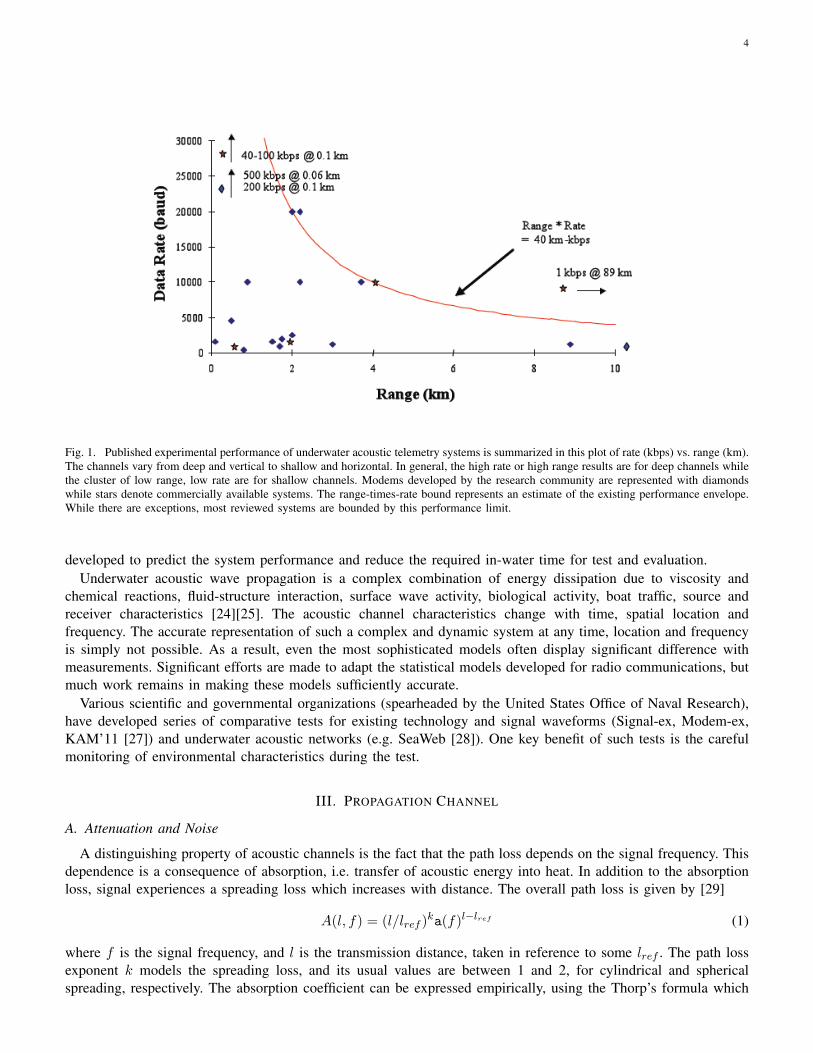
Fig. 1. Published experimental performance of underwater acoustic telemetry systems is summarized in this plot of rate (kbps) vs. range (km).The channels vary from deep and vertical to shallow and horizontal. In general, the high rate or high range results are for deep channels whilethe cluster of low range, low rate are for shallow channels. Modems developed by the research community are represented with diamondswhile stars denote commercially available systems. The range-times-rate bound represents an estimate of the existing performance envelope.While there are exceptions, most reviewed systems are bounded by this performance limit.

developed to predict the system performance and reduce the required in-water time for test and evaluation.Underwater acoustic wave propagation is a complex combination of energy dissipation due to viscosity and

chemical reactions, fluid-structure interaction, surface wave activity, biological activity, boat traffic, source andreceiver characteristics [24][25]. The acoustic channel characteristics change with time, spatial location andfrequency. The accurate representation of such a complex and dynamic system at any time, location and frequencyis simply not possible. As a result, even the most sophisticated models often display significant difference withmeasurements. Significant efforts are made to adapt the statistical models developed for radio communications, butmuch work remains in making these models sufficiently accurate.

Various scientific and governmental organizations (spearheaded by the United States Office of Naval Research),have developed series of comparative tests for existing technology and signal waveforms (Signal-ex, Modem-ex,KAM’11 [27]) and underwater acoustic networks (e.g. SeaWeb [28]). One key benefit of such tests is the carefulmonitoring of environmental characteristics during the test.

III. PROPAGATION CHANNEL

A. Attenuation and Noise

A distinguishing property of acoustic channels is the fact that the path loss depends on the signal frequency. Thisdependence is a consequence of absorption, i.e. transfer of acoustic energy into heat. In addition to the absorptionloss, signal experiences a spreading loss which increases with distance. The overall path loss is given by [29]

A(l, f) = (l/lref )ka(f)l−lref (1)

where f is the signal frequency, and l is the transmission distance, taken in reference to some lref . The path lossexponent k models the spreading loss, and its usual values are between 1 and 2, for cylindrical and sphericalspreading, respectively. The absorption coefficient can be expressed empirically, using the Thorp’s formula which

5

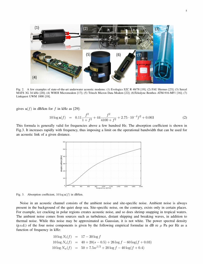
Fig. 2. A few examples of state-of-the-art underwater acoustic modems: (1) Evologics S2C R 48/78 [19]; (2) FAU Hermes [23]; (3) SercelMATS 3G 34 kHz [20]; (4) WHOI Micromodem [17]; (5) Tritech Micron Data Modem [22]; (6)Teledyne Benthos ATM-916-MF1 [16]; (7)Linkquest UWM 1000 [18].

gives a(f) in dB/km for f in kHz as [29]:

10 log a(f) = 0.11f2

1 + f2+ 44

f2

4100 + f2+ 2.75 · 10−4f2 + 0.003 (2)

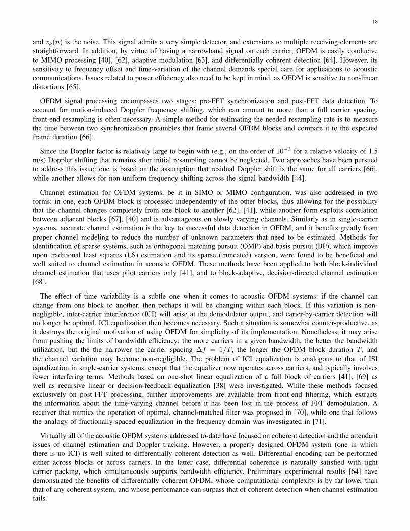
This formula is generally valid for frequencies above a few hundred Hz. The absorption coefficient is shown inFig.3. It increases rapidly with frequency, thus imposing a limit on the operational bandwidth that can be used foran acoustic link of a given distance.

0 20 40 60 80 100 120 140 160 180 2000

10

20

30

40

50

60

frequency [kHz]

abso

rption

coeff

icient

[dB/km

]

Fig. 3. Absorption coefficient, 10 log a(f) in dB/km.

Noise in an acoustic channel consists of the ambient noise and site-specific noise. Ambient noise is alwayspresent in the background of the quiet deep sea. Site-specific noise, on the contrary, exists only in certain places.For example, ice cracking in polar regions creates acoustic noise, and so does shrimp snapping in tropical waters.The ambient noise comes from sources such as turbulence, distant shipping and breaking waves, in addition tothermal noise. While this noise may be approximated as Gaussian, it is not white. The power spectral density(p.s.d.) of the four noise components is given by the following empirical formulae in dB re µ Pa per Hz as afunction of frequency in kHz:

10 logNt(f) = 17− 30 log f

10 logNs(f) = 40 + 20(s− 0.5) + 26 log f − 60 log(f + 0.03)

10 logNw(f) = 50 + 7.5w1/2 + 20 log f − 40 log(f + 0.4)

6

10 logNth(f) = −15 + 20 log f (3)

Fig.4 shows the total p.s.d. of the ambient noise for several values of the wind speed w (wind drives the surfacewaves which break and generate noise) and several levels of the distant shipping activity s ∈ [0, 1] (thousands ofships are present in the ocean at any time, and they generate distant noise which is to be distinguished from thesite-specific noise of vessels passing nearby). The noise p.s.d. decays at a rate of approximately 18 dB/decade,as shown by the straight dashed line in Fig.4. This line represents an approximate model for the noise p.s.d.,N(f) = N0 · (f/fref )−η. The parameters N0 and η can be fitted from the model, but also from the measurementstaken at a particular site.

100

101

102

103

104

105

106

20

30

40

50

60

70

80

90

100

110

f [Hz]

nois

e p.

s.d.

[dB

re

mic

ro P

a]

........ wind at 10 m/s

____ wind at 0 m/s

shipping activity 0, 0.5 and 1

(bottom to top)

Fig. 4. Power spectral density of the ambient noise. The dash-dot line shows an approximation 10 logN(f) =50dB re µ Pa−18log(f/1kHz).

The attenuation which grows with frequency, and the noise whose p.s.d. decays with frequency, result in a signal-to-noise ratio (SNR) which varies over the signal bandwidth. If one defines a narrow band of frequencies of width∆f around some frequency f , the SNR in this band can be expressed as

SNR(l, f) =Sl(f)∆f

A(l, f)N(f)∆f(4)

where Sl(f) is the p.s.d. of the transmitted signal. For any given distance, the narrowband SNR is thus a function offrequency, as shown in Fig.5. From this figure it is apparent that the acoustic bandwidth depends on the transmissiondistance. In particular, the bandwidth and the power needed to achieve a pre-specified SNR over some distance canbe approximated as B(l) = b·l−β and P (l) = p·lψ, where the coefficients b, p, and the exponents β ∈ (0, 1), ψ ≥ 1,depend on the target SNR, the parameters of the acoustic path loss and the ambient noise [30]. The bandwidth isseverely limited at longer distances: at 100 km, only about a kHz is available. At shorter distances, the bandwidthincreases, but it will ultimately be limited by that of the transducer. The fact that the bandwidth is limited impliesthe need for bandwidth-efficient modulation methods if more than a bps/Hz is to be achieved over these channels.

Another important observation to be made is that the acoustic bandwidth B is often on the order of the centerfrequency fc. This fact bears significant implications on the design of signal processing methods, as it prevents onefrom making the narrowband assumption, B << fc, on which many radio communication principles are based.Respecting the wideband nature of the system is particularly important in multi-channel (array) processing and insynchronization for mobile acoustic systems.

Finally, the fact that the acoustic bandwidth depends on the distance has important implications on the designof underwater networks. Specifically, it makes a strong case for multi-hopping, since dividing the total distance

7

0 2 4 6 8 10 12 14 16 18 20−170

−160

−150

−140

−130

−120

−110

−100

−90

−80

−70

5km

10km

50km

100km

frequency [kHz]

1/A

N [d

B]

Fig. 5. Signal-to-noise ratio in an acoustic channel depends on the frequency and distance through the factor 1/A(l, f)N(f). This figurerefers to the nominal SNR value that does not include variations induced by shadowing or multipath propagation.

between a source and destination into multiple hops enables transmission at a higher bit rate over each (shorter)hop. Since multi-hopping also ensures lower total power consumption, its benefits are doubled from the viewpointof energy-per-bit consumption on an acoustic channel [31]. Granted, by increasing the number of hops, the level ofinterference will increase, and packet collisions may become more likely, requiring in turn more re-transmissions.However, as shorter hops support higher bit rates, data packets containing a given number of bits will have shorterduration if the bit rate is appropriately increased, and the chances of collision will be reduced. This fact speaksfurther in favor of acoustic system design based on high-bandwidth, multi-hop links.

B. Multipath Propagation

While the basic propagation loss describes energy spreading and absorption, it does not take into account thespecific system geometry and the resulting multipath propagation. Multipath formation in the ocean is governed bytwo effects: sound reflection at the surface, bottom and any objects, and sound refraction in the water. The latter is aconsequence of sound speed variation with depth, which is mostly evident in deep water channels. Fig.6 illustratesthe two mechanisms.

Sound speed depends on the temperature and pressure, which vary with depth, and a ray of sound always bendstowards the region of lower propagation speed, obeying the Snell’s law. In shallow water, both the temperature andpressure are constant, and so is the sound speed. As the depth increases, the temperature starts to decrease, butthe weight of the water above is still not significant enough to considerably change the pressure. The sound speedthus decreases in the region called the main thermocline. After some depth, the temperature reaches the constantlevel of 4◦C, and from there on, the sound speed increases with pressure. When a source launches a beam of rays,each ray will follow a slightly different path, and a receiver placed at some distance will observe multiple signalarrivals. Note that a ray traveling over a longer path may do so at a higher speed, thus reaching the receiver beforea direct, stronger ray. This phenomenon results in a non-minimum-phase channel response.

The first approach to modeling multipath propagation is a deterministic one, which provides an exact solution forthe acoustic field strength in a given system geometry with a given sound speed profile. Because of computationalcomplexity, approximate solutions are often used instead of the exact ones. An approximation that is suitable forfrequencies of interest to acoustic communication systems is based on ray tracing. A widely-used package Bellhopis available online [32] (see also [33], [34]). Fig.7 illustrates a ray-trace obtained for a transmitter placed insidethe circle to the left. Lighter colors in this figure indicate locations of higher received signal strength. If a receiveris placed at some distance away from the transmitter in this field, the signal strength will vary depending upon theexact location. In other words, two receivers (e.g. two circles to the right) placed at the same distance away fromthe transmitter, may experience propagation conditions that are quite different. In this example, shadowing is causedby ray bending in deep water. In shallow water with constant sound speed, signal strength can be calculated usingsimple geometrical considerations. Alternating constructive/destructive combining of multiple reflections will nowform pockets of strong/weak signal reception. In either case, multipath effects make the signal strength location-

8

tx

distancec

tx rx

rx

depth

continental shelf (~100 m)

continental slice

continental rise

abyssal

plain

land sea

surf shallow deep

depth

c

surface layer (mixing)

const. temperature (except under ice)

main thermocline

temperature decreases rapidly

deep ocean

constant temperature (4 deg. C)

pressure increases

Sound speed increases with temperature, pressure, salinity.

~100 m

~600 m

~3000 m

deep ocean

trenches at 10 km

sound speed profile ocean cross-section

Fig. 6. Multipath formation in shallow and deep water (top). Sound speed as a function of depth and the corresponding ocean cross-section(bottom).

dependent, i.e. different from the value predicted by the basic propagation loss (1). If the transmitter or receiver wereto move through this frozen acoustic field, the received signal strength would be perceived as varying. In practice,of course, neither the channel geometry nor the environmental parameters are frozen, and small disturbances causethe signal strength to vary in time even if there is no intentional motion of the transmitter or receiver.

The impulse response of an acoustic channel is thus influenced by the geometry of the channel and its reflectionand refraction properties, which determine the number of significant propagation paths, their relative strengths anddelays. Strictly speaking, there are infinitely many signal echoes, but those that have undergone multiple reflectionsand lost much of the energy can be discarded, leaving only a finite number of significant paths.

To put a mathematical channel model in perspective, let us denote by lp the nominal length of the p-th propagationpath, with p = 0 corresponding to a reference path (either the strongest, or the first significant arrival). In shallowwater, where the sound speed c can be taken as constant, path delays can be obtained as τp = lp/c. Surfacereflection coefficient equals -1 under ideal conditions, while bottom reflection coefficients depend on the type ofbottom (hard, soft) and the grazing angle [35]. If we denote by Γp the cumulative reflection coefficient along thepth propagation path, and by A(lp, f) the propagation loss associated with this path, then

Hp(f) =Γp√

A(lp, f)(5)

represents the nominal frequency response of the p-th path. Hence, each path of an acoustic channel acts as alow-pass filter. Fig.8 illustrates a reference path transfer function H0(f) = 1/

√A(l0, f).

For the distances and frequencies of interest to the majority acoustic communication systems, the effect of pathfiltering is approximately the same for all paths, as the absorption coefficient does not vary much from its valueat the reference distance and center frequency. Denoting this value by a0, the transfer function of the p-th path ismodeled as

Hp(f, t) = hp ·H0(f) (6)

wherehp =

Γp√(lp/l0)ka

lp−l00

(7)

9

i

Fig. 7. A ray-trace shows areas of strong/weak signal reception. Sound reflection and refraction result in multipath propagation whichfavors some locations while placing others in a shadow.

−1 −0.8 −0.6 −0.4 −0.2 0 0.2 0.4 0.6 0.8 1

x 105

0

1

2

3

4

5

6x 10

−3

f [Hz]

refe

renc

e pa

th tr

ansfe

r fun

ction

Fig. 8. Reference path transfer function H0(f). Path length l0=1 km, spreading factor k = 1.5.

is the real-valued (passband) path gain. Fig.9 shows an example of nominal multipath structure.In an acoustic communication system, the channel can be observed only in a limited band of frequencies supported

by the transducer. As a result, the observable response will be smeared, as illustrated in Fig.10. It is important tomake the distinction between the natural channel paths of the channel (Fig.9), and the samples of the observableresponse (Fig.10). The latter are often referred to as the channel taps. It is also important to note that the pathgains can be very stable, while taps may exhibit fast variation. Such behavior is explained by the fact that eachtap contains contributions from all the paths, wherein each path carries a pulse of finite duration and a differentdelay that is varying in time. An example of tap variation is shown in Fig.13, which we will discuss later whenwe address channel fading.

Multipath propagation creates a frequency-selective channel distortion, which is evident as the variation of thetransfer function in Fig.10. As a result, some frequencies of a wideband acoustic signal will be favored, while

10

−0.5 0 0.5 1 1.5 2 2.5 3 3.5 4 4.5 5

−1

−0.8

−0.6

−0.4

−0.2

0

0.2

0.4

0.6

0.8

1

nominal path gains

delay [ms]

Fig. 9. Nominal path gains (7) for a channel with transmission distance d=1 km, water depth h=20 m, and transmitter/receiver heightabove the bottom hT =10 m and hR=12 m. Spreading factor is k=1.5, surface reflection coefficient is -1; bottom reflection coefficients arecalculated assuming speed of sound and density of c=1500 m/s, ρ=1000 g/m3 in water and cb=1300 m/s, ρb=1800 g/m3 in soft bottom.Those paths whose absolute value is above one tenth of the strongest path’s are shown.

0 1 2 3 4 50

0.2

0.4

0.6

0.8

1

delay [ms]

imp

uls

e r

esp

on

se m

ag

nitu

de

10 11 12 13 14 15 16 17 18 19 200

0.2

0.4

0.6

0.8

1

frequency [kHz]

tra

nsf

er

fun

ctio

n m

ag

nitu

de

Fig. 10. Impulse response (baseband) and the transfer function for the nominal (time-invariant) channel geometry corresponding to themultipath structure of Fig.9, as seen in B=10 kHz of bandwidth centered at fc=15 kHz. In a wideband acoustic system, multipath propagationcreates discernible signal echoes and a frequency-selective channel distortion.

others will be severely attenuated. Channel equalization has to be employed to deal with this type of distortion.The total delay spread between significant multipath arrivals, or the multipath spread of the channel, Tmp, is an

important figure of merit for the design of acoustic communication systems. Vertical links exhibit short multipathspreads, while horizontal channels exhibit multipath spreads that can range between a few ms and hundreds ofms. In single-carrier broadband systems, where the data symbols are short compared to the multipath spread, themeaningful figure of merit is the number of symbols that fit within the multipath spread. This number determinesthe extent of inter-symbol interference (ISI), which in turn dictates the length of the filters needed to equalize thechannel. The fact that the multipath spread may be on the order of several ms, or more, implies that the ISI mayspan tens or even a hundred symbol intervals, a situation very different from that typically found in radio systems,where ISI may involve a few symbols only. Multi-carrier systems avoid this problem by transmitting in parallel onmany carriers, each occupying a narrow sub-band. A meaningful figure of merit for these systems is the frequencycoherence, ∆fcoh = 1/Tmp. In a properly designed multi-carrier system, carrier separation is kept well below this

11

value.The acoustic channel is often sparse, i.e. there are only several significant paths that populate the total and possibly

long delay spread. This fact has an important implication on channel estimation and the associated equalizationmethods. Namely, while the entire multipath spread is represented by L ∼ TmpB samples taken at intervalsTs = 1/B, fewer than L coefficients may suffice to represent the channel response. Ideally, only as many coefficientsas there are propagation paths, P < L, are needed. Channel modeling thus becomes an important aspect of signalprocessing, and sparsing has been investigated for decision-feedback equalization [36], [37], turbo equalization[38], [39], and multi-carrier detection [40], [41], [42]. It is also important to note that although a greater bandwidthimplies more ISI and more frequency selectivity, it also implies a better resolution in delay (less smearing in theobservable channel response). Hence, although the attendant signal distortion is perceived as more severe, channelestimation will be more efficient if a proper sparse model is used, which may in turn lead to improved signalprocessing. In addition, signaling at a higher rate enables more frequent channel observations and, consequently,easier channel tracking [43].

C. Time Variability: Motion-Induced Doppler Distortion

There are two sources of the channel’s time variability: inherent changes in the propagation medium whichcontribute to signal fading, and those that occur because of the transmitter/receiver motion and contribute to thefrequency shifting. The distinction between the two types of distortions is that the first one appears as random,while the motion-induced Doppler effects can me modeled in a deterministic manner and therefore compensatedto some degree through synchronization.

Motion of the transmitter, receiver, or a reflection point along the signal path causes the path distances tovary with time. The resulting Doppler effect is evident as time compression/dilation of the signal, which causesfrequency shifting and bandwidth spreading/shrinking. The magnitude of the Doppler effect is proportional to theratio a = v/c of the relative transmitter-receiver velocity to the speed of sound. Because the speed of sound is verylow as compared to the speed of electro-magnetic waves, motion-induced Doppler distortion of an acoustic signalcan be extreme. AUVs move at speeds that are on the order of a few m/s, but even without intentional motion,underwater instruments are subject to drifting with waves, currents and tides, which may occur at comparablevelocities. In other words, there is always some motion present in the system, and a communication system has tobe designed taking this fact into account. The only comparable situation in radio communications occurs in the lowEarth orbiting (LEO) satellite systems, where the relative velocity of satellites flying overhead is extremely high(the channel there, however, is not nearly as dispersive in delay). The major implication of the motion-induceddistortion is on the design of synchronization algorithms.

To model the Doppler distortion, let us focus on a single propagation path, assuming that the relativetransmitter/receiver velocity vp along this path stays constant over some interval of time. The path delay canthen be modeled as

τp(t) = τp − ap · t (8)

where ap = vp/c is the Doppler factor corresponding to the p-th path. If there is a single dominant componentof velocity, these factors can be approximated as equal for all paths, ap = a, ∀p; however, this is not the case ingeneral [37]. To assess the effect oftime-varying delay on the signal, let us focus on a particular signal componentcentered around frequency fk in a narrow band ∆f ≪ fk. The signal sk(t) and its equivalent baseband uk(t) arerelated by

sk(t) = Re{uk(t)ej2πfkt} (9)

Since the signal occupies only a narrow band of frequencies, its replica received over the p-th propagation path isgiven by

sk,p(t) = hpQ(fk)sk(t− τp(t)) (10)

Defining the equivalent baseband component of the received signal via

sk,p(t) = Re{vk,p(t)ej2πfkt} (11)

we have the baseband relationship

vk,p(t) = ck,pej2πapfktuk(t+ apt− τp) (12)

12

where ck,p is constant,ck,p = hpH0(fk)e

−j2πfkτp (13)

and the Doppler effect is evident in two factors: (i) frequency shifting by the amount apfk, and (ii) time scaling bythe factor (1+ap). Putting together all the signal components at frequencies f0, f1, etc., that span a wide bandwidthB = K∆f , and assuming only a single propagation path with the Doppler factor a, the situation is illustrated inFig.11. This figure offers an exaggerated view of the Doppler effect, but nonetheless one that suffices to illustratethe point: each spectral component in a wideband mobile acoustic system is shifted by a different amount, and thetotal bandwidth B is spread over B(1+a), i.e. a signal of duration T is observed at the receiver as having durationT/(1 + a).

f

…

B=K f

f

f

fk fk(1+a)

Fig. 11. Motion-induced Doppler shift is not uniform in a wideband acoustic system.

The way in which these distortions affect signal detection depends on the actual value of the factor a. Forcomparison, let us look at a highly mobile radio system: at 160 km/h (100 mph), a = 1.5 · 10−7. This value islow enough that Doppler spreading can be neglected. In other words, there is no need to account for it explicitlyin symbol synchronization. The error made in doing so is only 1/1000 of a bit per 10,000 bits. In contrast tothis situation, a stationary acoustic system may experience unintentional motion at 0.5 m/s (1 knot), which wouldaccount for a = 3 · 10−4. For an AUV moving at several m/s (submarines can move much faster), the factor a willbe on the order of 10−3, a value that cannot be ignored.

Non-negligible motion-induced Doppler shifting and spreading thus emerge as another major factor thatdistinguishes an acoustic channel from the mobile radio channel, and dictates the need for explicit phase and delaysynchronization in all but stationary systems [10]. In multi-carrier systems, Doppler effect creates a particularlysevere distortion. Unlike in the radio systems, where time compression/dilation is negligible and the Doppler shiftappears equal for all frequencies within the signal bandwidth, in an acoustic system each frequency componentmay experience a markedly different Doppler shift, creating a non-uniform Doppler distortion across the signalbandwidth [44].

D. Time Variability: Random Effects (Fading)

Inherent channel changes range from the very large-scale, slow variations that occur seasonally (e.g. the change insound speed profile from winter to summer) or daily (e.g. the change of water depth due to tides) to the small-scale,fast variations that are often caused by the rapid motion of the sea surface (waves) or the system itself. Many ofthese variations appear as random, and as such require an additional stage of modeling, namely statistical modeling.

The distinction between various scales is meaningful from the viewpoint of the duration of communicationsignals. While the large-scale phenomena affect average signal power, causing it to vary over longer periods oftime (many data packets), small-scale phenomena affect the instantaneous signal level, causing it to vary overshorter periods of time (few data packets, or bits of the same data packet). In light of system design, it is alsouseful to distinguish between those variations that are slow enough to admit a feedback by which the receivercan inform the transmitter of the change, and those that are too fast to be conveyed over the time it takes thesignal to propagate from one end of the link to another. In this sense, modeling of the large-scale phenomenais meaningful for adaptive power control and modulation (which are performed at the transmitter in response todelayed feedback), while modeling of the small-scale phenomena is important for adaptive signal processing at the

13

receiver (channel estimation, equalization). It is also important to note that the apparently random channel variationcan be a consequence of both the changes in the physical parameters of the environment (sounds speed profile,surface scattering, internal waves) and the changes in the placement of the system within a given environment(transmitter/receiver displacement due to intentional motion or drifting with currents, etc.). Note also that theseeffects will differ across different environments, e.g. deep or shallow water, tropical or ice-covered regions.

1) large-scale effects: To assess the random variation of the channel, one can start by allowing the path lengthsto deviate from the nominal values, so that

lp = lp +∆lp (14)

where ∆lp is regarded as a random displacement. This displacement models the large-scale variation which occursbecause the channel geometry deviates from the nominal, either as the system is moved to a different location, orbecause the water depth has changed with tide, etc. The deterministic, motion-induced delay variation which canbe compensated through proper synchronization, is not consider as part of statistical channel analysis.The resultingtransfer function of the channel, which in now random as well, is given by

H(f) = H0(f)∑p

hpe−j2πfτp (15)

where the path coefficients hp can be calculated similarly as for the nominal case (7), using lp instead of lp, andthe delays can be calculated as τp = lp/c− t0 in reference to some time, e.g. t0 = l0/c. The corresponding randompath gains can also be approximated as [45]

hp = hpe−ξp∆lp/2 (16)

whereξp = ac − 1 + k/lp (17)

and hp is given by the expression (7). Note that one can also explicitly express the salient parameters hp, τp asfunctions of time, i.e. hp(t), τp(t), if one is interested in their variation during a long-term deployment in the samearea (deep/shallow water, etc.).

2) Small-scale effects: The above model accounts only for the variations induced by the path length displace-ments, i.e. it does not include the effects of scattering. Scattering, which causes micro-path dispersion along eachpropagation path, can be modeled through an additional factor that accompanies the path gain hp(t). An overallchannel model is now obtained in the form

H(f, t) = H0(f)∑p

γp(f, t)hp(t)e−j2πfτp(t) (18)

In this model, the factors hp(t) account for the slower-changing process caused by the deviations of the systemgeometry from the nominal, while the factors γp(f, t) represent the faster-changing scattering process. In otherwords, during a typical communication transaction of several packets, the path gains can be considered fixed, hp(t) =hp, but the additional factors γp(f, t) cannot. These factors are often modeled as circularly-symmetric complex-valued Gaussian processes, and are normalized so as not to alter the total received signal power, i.e. E{|γp(f, t)|2} =1. In general, scattering in an acoustic channel depends on the signal frequency, making each macro-path experiencea different, possibly independent filtering effect. Note, however, that the transfer function H(f, t) will in generalexhibit correlation in both frequency and time (as well as across the elements of a transmit/receive array).

3) Statistical characterization: Because of the different dynamics of the two types of processes, statistical channelanalyses are typically conducted in two forms: one that targets the locally-averaged received signal power, andanother that targets the instantaneous channel response. Specifically, large-scale statistical modeling focuses on thechannel gain defined as

G(t) =1

B

∫ fc+B/2

fc−B/2Eγ{|H2(f, t)|}df (19)

where the expectation is taken over small-scale fading. In contrast, small-scale modeling focuses on the processesγp(f, t), i.e. on the channel response conditioned on the large-scale parameters hp(t) and τp(t).

A complete statistical model for either large or small scale phenomena must specify the probability densityfunction (p.d.f.) and the power spectral density (p.s.d.) or the correlation properties of the random process of

14

interest. These functions can be assessed using an analytical approach that relies on a mathematical model suchas the one outlined above; a repeated application of a propagation model such as the Bellhop ray tracer for alarge number of slightly disturbed channel conditions, or an experimental data analysis. All approaches have beenconsidered in the literature, which abounds in statistical models that were found to adequately match the channelsobserved in different locations, at different time scales, and in different frequency bands. As of this time, however,the jury is still out on establishing standard models that would concisely describe the statistics of typical underwateracoustic channels. Crucial to that effort is identification of the scales of stationarity for the different processes athand.

As far as the large-scale modeling goes, recent experimental results offer some evidence in support of a log-normal model for the channel gain [46], [47],[45]. Fig.12 illustrates such a model. Several of these studies also findthat the path gains, and consequently the overall large-scale channel gain, can be well modeled as auto-regressiveprocesses, at least on the time scales of several seconds, which are meaningful for implementation of packet-levelfeedback schemes.

Experimental studies of the small scale fading have offered evidence to Ricean [46], [48], [49] as well as Rayleighphenomena [50]. Fig.13 illustrates an experimental data set that exhibits traits of Ricean fading. Combining theeffects of large- and small-scale fading leads to a mixture of log-normal and Ricean distributions, which can beapproximated in closed form by the compound K-distribution. Experimental evidence to this effect is providedin Ref.[51]. Less is known about modeling the time-correlation functions of the small-scale processes, but it isgenerally understood that coherence times on the order of 100 ms can be assumed for a general-purpose design.Frequency-correlation as well as space-correlation, as they pertain to communications systems, also remain to beaddressed in a systematic manner.

100 200 300 400 500 600 700 800 900 10005

10

15

20

25

30

distance [m]

gain

[dB

]

gg

0−k

010 log d

−15 −10 −5 0 5 10 150

0.02

0.04

0.06

0.08

0.1

0.12

0.14

0.16

x [dB]

pdf

Fig. 12. During an experiment off the coast of Northern California, an acoustic signal occupying the 8-12 kHz band was transmitted betweena fixed station and an AUV, and the strength of the signal receiver by the WHOI micro-modem was measured over a period of time duringwhich the transmission distance changed. The figure on the left shows the recorded signal strength, i.e. an estimate of the channel gain (19),as a function of distance (dots) and the accompanying trend which exhibits a log-distance dependence (solid). The figure on the right showsthe histogram of the difference between the recorded gain and the nominal trend, which is well described by a Gaussian distribution on thedB scale, i.e. a log-normal distribution on the linear scale.

The importance of statistical channel modeling is twofold. On the one hand, it enables the design of practicaladaptive modulation methods which rely on identifying those channel parameters that can be predicted via a delayedreceiver-transmitter feedback [52]. On the other hand, it will enable the development standardized simulation models,thus allowing performance analysis not only of signal processing methods, but also of network protocols and system-level design strategies, without the need for actual system deployment. Currently available simulators, such as theWorld Ocean Simulation System [53], use accurate ray tracing models, but they lack the statistical aspect of assessingthe system performance.

E. System Constraints

In addition to the fundamental limitations imposed by acoustic propagation, there are hardware constraints thataffect the operation of acoustic modems. The most obvious of these constraints is the fact that acoustic transducers

15

have their own bandwidth limitation, which constraints the available bandwidth beyond that offered by the channel.Additional constrains include power efficiency (transmit amplifiers are often non-linear, imposing a limit on thepeak signal power), and the fact that acoustic modems operate in half-duplex fashion. These constraints do not affectonly the physical link, but all the layers of a network architecture. For example, half-duplex mode of operation,combined with the low speed of sound, challenges the throughput efficiency of acoustic links that require automaticrepeat request (ARQ) [54].

In an acoustic system, the power required for transmitting may be much greater than the power required forreceiving. Transmission power depends on the distance, and its typical values are on the order of tens of Watts. (Anacoustic signal propagates as a pressure wave, whose power is measured in Pascals, or commonly in dB relative toa micro Pascal. In seawater, 1 Watt of radiated acoustic power creates a sound field of intensity 172 dB re µPa 1 mmeter away from the source.) In contrast, the power consumed by the receiver is much lower, with typical valuesranging from about 100 mW for listening or low-complexity detection, to no more than a few Watts required toengage a sophisticated processor for high-rate signal detection. In hybernation mode, from which a modem can bewoken on command, no more than 1 mW is required.

Underwater instruments are often battery-powered, and, hence, it is not simply the power, but the energyconsumption that matters. This is less of an issue for mobile systems, where the power used for communication is asmall fraction of the total power consumed for propulsion, but it is important for networks of fixed bottom-mountednodes, where the overall network lifetime is the figure of merit. One way to save the energy is by transmittingat a higher bit rate. For example, the WHOI modem [55] has two modes of operation: high rate at 5 kbps andlow rate at 80 bps. This modem will require about 60 times less energy per bit (18 dB) in the high-rate mode.The receiver’s energy consumption will also be lower, although it requires 3 W for detection of high-rate signalsas opposed to 80 mW for detection of low-rate signals (the difference is about 2 dB). Another way to save theenergy is by minimizing the number of retransmissions (we discuss the relevant protocols in Sec.IV-F). Finally,energy spent in idle listening over a longer period of time is not to be neglected. Having modems that are capableof hybernation, or instituting intentional sleeping schedules for those that are not, can help to control this type ofpower expenditure [56].

IV. POINT TO POINT LINKS: SIGNAL PROCESSING

A. Noncoherent Modulation/Detection

Noncoherent signaling is commonly used to relay data and to transmit command-and-control information at lowbitrate. Frequency-Hopped M-ary Frequency-Shift-Key (FH-MFSK) modulation is widely accepted as a reliablealbeit inefficient choice for such modems. FSK modulation uses distinct tonal or frequency-modulated pulsesto map digital information. Frequency-hopping is a spread-spectrum technique, which alternates portions of thefrequency band over fixed periods of time, so that successive FSK-modulated symbols use a different portion of thefrequency spectrum, thus minimizing Inter-Symbol-Interference (ISI) caused by reverberation. Many commercialsuppliers offer several versions of FH-MFSK acoustic modems. In the case of a combination of N tones transmittedsimultaneously, the symbol transmitted during the m-th signaling interval (mTs ≤ t < (m+ 1)Ts) is

sm(t) = Amd(t)N∑n=1

gm,ncm,n(t),mTs ≤ t < (m+ 1)Ts, (20)

where, in the simplest case, cm,n(t) is a tone (either real or complex),

cm,n(t) = e2πjfm,n(t−mTs),mTs ≤ t < (m+ 1)Ts. (21)

Am is the peak acoustic pressure of symbol sm(t). d(t) is the pulse shape (e.g. Gaussian). Ts is the pulse durationin seconds. fm,n is the carrier frequency of tone n for symbol sm(t). The binary information b(m) is coded insymbol sm(t) as a combination gm,n of frequency bands centered at fm,n(n = 1, ..., N). gm,n = 1 if the frequencyband is used, otherwise gm,n = 0 (at least one band is used for every symbol sm(t)). If sm(t) uses only one ofN bands and N is a power of 2, log2(N) bits can be coded simultaneously within a single symbol. For example,if N = 4, sm(t) will contain log2(4) = 2 bits of binary information (b(m) =(0,0),(0,1),(1,0) or (1,1)). If g1,n = 1

16

and g2,n = g3,n = g4,n = 0, then bm = (0, 0). If g2,n = 1 and g1,n = g3,n = g4,n = 0, then bm = (0, 1) and so on.Fig.14 shows a section of an FH-MFSK modulated signal and the corresponding periodogram.

At the receiver, the incoming message is first detected and synchronized using a short FH-MFSK modulatedsequence. Following this, each data symbol is processed individually. First, the cross-correlation between theincoming faded symbol and a set of reference symbols cm,n(t) is computed,

Rrm,cm,n(τ) =

∫ Ts

−Ts

rm(t)c∗m,n(t+ τ)dt, (22)

where ∗ denotes the complex conjugate. For every received symbol rm(t), we retain the peak of correlation withineach band centered at fm,n,

Zm,n = maxt{Rrm,cm,n

(τ);mTs ≤ t < (m+ 1)Ts}. (23)

If we assume once more that sm(t) uses only one of N bands and N is a power of 2, we identify the frequencyband that contains the most energy by comparing the coefficients Zm,n,

nmax(m) = maxn {Zm,n;n = 1, ..., N} . (24)

Note that nmax is a function of the symbol index m. Under the same assumption, gm,n = 1 if n = nmax, otherwisegm,n = 0. For example, if nmax = 1, then gm,1 = 1 and gm,2 = gm,3 = gm,4 = 0. Therefore, sm(t) contains thecouple of bits bm = (0, 0). If nmax = 2, then gm,2 = 1 and gm,1 = gm,3 = gm,4 = 0, so that sm(t) contains thecouple of bits bm = (0, 1), and so on.

B. Coherent Modulation/Detection

Coherent modulation methods include phase shift keying (PSK) and quadrature amplitude modulation (QAM).These methods offer bandwidth efficiency, i.e. the possibility to transmit more than one bit per second per Hertzof occupied bandwidth. However, because the information is encoded into the phase or amplitude of the signal,precise knowledge of the received signal’s frequency and phase is required in order to perform coherent detection.This fact presents a major challenge because an acoustic channel introduces a rather severe phase distortion oneach of its multiple paths. A coherent receiver thus needs to perform phase synchronization together with channelequalization.

Coherent systems fall into two types: single-carrier and multi-carrier systems. In single-carrier systems, abroadband information-bearing signal is directly modulated onto the carrier and transmitted over the channel.A typical high-rate acoustic signal occupies several kHz of bandwidth over which it experiences uneven channeldistortion (see Fig.10). This distortion must be compensated at the receiver through the process of equalization.Multi-carrier modulation bypasses this problem by converting the high-rate information stream into many parallellow-rate streams, which are then modulated onto separate carriers. The carriers are spaced closely enough such thatthe channel appears as frequency-flat in each narrow sub-band. After demodulation, each carrier’s signal now onlyhas to be weighted and phase-synchronized, i.e. a single-coefficient equalizer suffices per carrier. Each of thesemethods has its advantages and disadvantages when it comes to practical implementation: single-carrier systems arecapable of faster channel tracking but they need high-maintenance equalizers; multi-carrier systems are efficientlyimplemented using the fast Fourier transform (FFT), but they have high sensitivity to residual frequency offsets. Inwhat follows, we review the basics of both types of systems as they apply to phase-distorted frequency-selectiveacoustic channels, and we outline the current research trends.

1) Single-carrier Modulation/Detection: The problem of joint phase tracking and equalization in single-carrierbroadband systems was addressed in Ref.[10]. The basic receiver structure [10] was extended to multichannel(array) configuration [57], [58] to enable diversity combining, which is often essential on acoustic channels. Theresulting multichannel decision-feedback equalizer (DFE), integrated with a second-order phase-locked loop (PLL),provided the benchmark design for the high-speed acoustic modem [55]. It also became a de-facto standard forthe development and comparison of future techniques, which focused on replacing the basic DFE with moresophisticated equalization and channel estimation schemes (e.g. turbo equalization and sparse channel estimation

17

[39]), or on inclusion of multiple transmitters, be it in the form of multi-user systems [59], [60] or multi-inputmulti-output (MIMO) structures for spatial multiplexing and/or diversity [61], [38].

The block diagram of a multi-channel DFE is shown in Fig.15. The receiver includes several stages: pre-combining (which may or may not be used, depending upon the array structure), phase correction, and multichannelequalization. The receiver is designed to process an incoming signal of the form

v(t) =∑n

d(n)gc(t− nT )ejθ(t) + w(t) (25)

where d(n) are the data symbols transmitted at the rate of one symbols per T ; gc(t) = gT (t) ∗ c(t) ∗ gR(t) is thecomposite impulse response of the transmitter, channel and receiver (all in equivalent baseband with respect to thecarrier frequency fc); θ(t) is the carrier phase, and w(t) is the noise. The channel response c(t) and the phaseθ(t) are unknown (and possibly different across the array elements), necessitating an adaptive receiver. Adaptiveequalization has been considered in two forms: direct, which does not perform explicit channel estimation, andindirect, in which the channel is first estimated and then used to adjust the equalizer. In either form, the datasymbols are estimated as

d̂(n) =P∑p=1

aHp (n)xp(n)e−jθ̂p(n) −

∑i>0

b∗i (n)d(n− i) (26)

where the input vector xp(n) to the p-th equalizer branch consists of the sampled pre-combiner output xp(t) =∑Kk=1 c

∗p,kv

(k)(t). The samples are taken at the Nyquist rate, e.g. two per symbol interval for signals band-limited to±1/T . The pre-combiner coefficients cp,k, the feedforward equalizer vectors ap, the feedback equalizer coefficientsbi, and the phase estimates θ̂p are adjusted adaptively so as to minimize the mean squared error (MSE) in datadetection. Each of these parameters is thus driven by the input signal and the error e(n) = d(n)− d̂(n). Adaptiveoperation begins with a training sequence of known data symbols d(n) until convergence has been established, afterwhich the symbols d(n) in Eq.(26) are replaced by the decisions d̃(n) made on the estimates d̂(n). The details ofvarious algorithm variants can be found in [57], [58], [36].

Performance of the multichannel DFE is illustrated in Fig.16. Excellent performance achieved by this receiveron many channels testifies to the benefits of careful algorithm structuring that caters to the acoustic channel. Whilea propagation-ignorant design may result in an unnecessarily large number of receiver parameters (many equalizerbranches with long filters) which will in turn cause increased sensitivity to noise and numerical errors, results similarto those of Fig.16 show that one may not need more equalizer branches than there are significant propagation paths;that each of these branches may not need an excessively long filter, and that the feedback filter may only needto activate a select subset of coefficients although its total span must match that of the multipath. In other words,respecting the physical aspects of acoustic propagation in developing a concise channel representation is the keyfor successful signal processing. Identification of “significant” channel components has attracted due interest in theacoustic community over the past several years, and much attention has been devoted to the topic of sparse channelestimation. Ref.[37] gives an excellent primer.

2) Multi-carrier Modulation/Detection: Multi-carrier modulation in the form of orthogonal frequency divisionmultiplexing (OFDM) has been adopted as a standard for many of the emerging wireless radio systems – wirelesslocal area networks (WLAN), digital audio and video broadcast (DAB/DVB), and long term evolution (LTE) thatwill support future generations of cellular systems. However, it has only recently come into the forefront of acousticcommunications research, and at the moment, there appear to be few efforts to implement this technology in acommercial modem (e.g. by the French Thales).

The appeal of OFDM lies in the computational efficiency of FFT-based processing, and in the fact that it easilyscales to different bandwidths (unlike with single-carrier systems, where the equalizer length has to be adjustedin accordance with the bandwidth B because it determines the symbol duration and hence the extent of ISI, withOFDM it simply suffices to increase/decrease the number of carriers K, i.e. the size of the FFT, while keeping thesame carrier separation ∆f = B/K). Namely, the demodulated signal in the k-th carrier, during the n-th block, issimply represented as

yk(n) = Hk(n)dk(n) + zk(n) (27)

where dk(n) is the data symbol transmitted on the k-th carrier during the n-th OFDM block of duration T = 1/∆f ;Hk(n) is the channel transfer function H(f, t) evaluated at the k-th carrier frequency at the time of the n-th block,

18

and zk(n) is the noise. This signal admits a very simple detector, and extensions to multiple receiving elements arestraightforward. In addition, by virtue of having a narrowband signal on each carrier, OFDM is easily conduciveto MIMO processing [40], [62], adaptive modulation [63], and differentially coherent detection [64]. However, itssensitivity to frequency offset and time-variation of the channel demands special care for applications to acousticcommunications. Issues related to power efficiency also need to be kept in mind, as OFDM is sensitive to non-lineardistortions [65].

OFDM signal processing encompasses two stages: pre-FFT synchronization and post-FFT data detection. Toaccount for motion-induced Doppler frequency shifting, which can amount to more than a full carrier spacing,front-end resampling is often necessary. A simple method for estimating the needed resampling rate is to measurethe time between two synchronization preambles that frame several OFDM blocks and compare it to the expectedframe duration [66].

Since the Doppler factor is relatively large to begin with (e.g., on the order of 10−3 for a relative velocity of 1.5m/s) Doppler shifting that remains after initial resampling cannot be neglected. Two approaches have been pursuedto address this issue: one is based on the assumption that residual Doppler shift is the same for all carriers [66],while another allows for non-uniform frequency shifting across the signal bandwidth [44].

Channel estimation for OFDM systems, be it in SIMO or MIMO configuration, was also addressed in twoforms: in one, each OFDM block is processed independently of the other blocks, thus allowing for the possibilitythat the channel changes completely from one block to another [62], [41], while another form exploits correlationbetween adjacent blocks [67], [40] and is advantageous on slowly varying channels. Similarly as in single-carriersystems, accurate channel estimation is the key to successful data detection in OFDM, and it benefits greatly fromproper channel modeling to reduce the number of unknown parameters that need to be estimated. Methods foridentification of sparse systems, such as orthogonal matching pursuit (OMP) and basis pursuit (BP), which improveupon traditional least squares (LS) estimation and its sparse (truncated) version, were found to be beneficial andwell suited to channel estimation in acoustic OFDM. These methods have been applied to both block-individualchannel estimation that uses pilot carriers only [41], and to block-adaptive, decision-directed channel estimation[68].

The effect of time variability is a subtle one when it comes to acoustic OFDM systems: if the channel canchange from one block to another, then perhaps it will be changing within each block. If this variation is non-negligible, inter-carrier interference (ICI) will arise at the demodulator output, and carier-by-carrier detection willno longer be optimal. ICI equalization then becomes necessary. Such a situation is somewhat counter-productive, asit destroys the original motivation of using OFDM for simplicity of its implementation. Nonetheless, it may arisefrom pushing the limits of bandwidth efficiency: the more carriers in a given bandwidth, the better the bandwidthutilization, but the the narrower the carrier spacing ∆f = 1/T , the longer the OFDM block duration T , andthe channel variation may become non-negligible. The problem of ICI equalization is analogous to that of ISIequalization in single-carrier systems, except that the equalizer now operates across carriers, and typically involvesfewer interfering terms. Methods based on one-shot linear equalization of a full block of carriers [41], [69] aswell as recursive linear or decision-feedback equalization [38] were investigated. While these methods focusedexclusively on post-FFT processing, further improvements are available from front-end filtering, which extractsthe information about the time-varying channel before it has been lost in the process of FFT demodulation. Areceiver that mimics the operation of optimal, channel-matched filter was proposed in [70], while one that followsthe analogy of fractionally-spaced equalization in the frequency domain was investigated in [71].

Virtually all of the acoustic OFDM systems addressed to-date have focused on coherent detection and the attendantissues of channel estimation and Doppler tracking. However, a properly designed OFDM system (one in whichthere is no ICI) is well suited to differentially coherent detection as well. Differential encoding can be performedeither across blocks or across carriers. In the latter case, differential coherence is naturally satisfied with tightcarrier packing, which simultaneously supports bandwidth efficiency. Preliminary experimental results [64] havedemonstrated the benefits of differentially coherent OFDM, whose computational complexity is by far lower thanthat of any coherent system, and whose performance can surpass that of coherent detection when channel estimationfails.

19

C. Data link reliabilityChannel coding or Forward Error Coding (FEC) in a crucial feature of underwater acoustic modems. By

introducing a redundancy part in the transmitted message, error correction codes allow for detection and correctionof the bit errors caused by noise and inter-symbol interference. Generally, the ability to correct the errors isachieved by adding redundancy, which in turns reduces the effective data rate. Therefore, a proper coding schemefor a communication system is chosen based on the trade-off between the desired data bit rate and error rateperformance.

Traditional FEC techniques are divided into convolutional codes (usually decoded with the ubiquitous Viterbialgorithm) and block codes (e.g. Bose-Chaudhuri-Hocquenghem or BCH, Reed-Solomon or RS) [72][73]. Concate-nated codes usually combine convolutional and block codes to improve even further the reliability of the acousticmodem. More recently, turbo codes [74][75] and Low-Density Parity-Check (LDPC) codes [76] have become part ofthe field of telecommunication as they offer near Shannon error correction capability. Having inherently a low codingrate and a potentially large decoding latency, turbo codes have emerged as a good choice in the communicationsystems where achieving a very low error rate performance is a top priority. A communication link designed forthe transmission of the command-and-control messages to a remotely operated robot or vehicle is such a system.Since control messages do not contain a large number of bits that need to be transmitted in a short time, high bitrates are not required.

Even the most sophisticated error codes cannot ensure complete link reliability. To guarantee an error-freecommunication link (if it is physically possible), the acoustic modem must include a Quality of Service (QoS)feature, typically in the form of an Automated Retransmission Query (ARQ) process implemented between twoacoustic modems [54][?]. This operation requires a communication protocol that includes acknowledgments andmay dramatically reduce the overall data rate. The optimization of the QoS protocol is a key feature of modernacoustic modems. Acoustic modem users should be aware that commercially advertised throughputs (data rates)assume a single message transmission and do not include any retransmission.

D. Turbo equalizationTurbo equalization is a very powerful method used to improve the removal of inter-symbol interference and

additive noise. This technique can be implemented with single-carrier and multiple-carrier signaling. In particular,extensive research in combining turbo equalization and OFDM has taken place over the past decade. The simplestand best explanation is provided in the seminal work published in [77]. In short terms, turbo-equalization jointlyoptimizes adaptive equalization and channel decoding in an iterative process. The result is a dramatic improvementof transmission quality, even for high spectral efficiency modulations and time-varying fading channels. Modernunderwater acoustic modems make a growing use of this technique, which is powerful but processor-intensive.

At the heart of this process is interleaving and error coding. The binary information at the source is carefullyerror-coded, modulated and interleaved before it is pulse-shaped and transmitted through the water channel. In atraditional equalized receiver, the distorted signal is equalized, deinterleaved, converted to the binary domain, theerror-coded binary information is decoded and hopefully every binary error is corrected.

The obvious issue with this method is the fact that some error may remain. The turbo-equalizer goes two stepsfurther in using this information. First of all, it modulates and interleaves the error-corrected binary information(which may still contain errors), thus cleaning the signal of some (or most of the) inter-symbol interference. Theoriginal signal is equalized once again, but this time the ”cleaned” signal is used as a new reference in the decisionfeedback portion of the adaptive equalizer. The second step is to repeat the entire operation again and again, sothat the original signal is equalized against an ever ”cleaner” reference signal.

The statistical properties of the acoustic channel, the type of interleaver, error coding and decoding have a signicantimpact on turbo-equalizers. However, the same can be said of every equalized communication system, and overallthis technique can lead to significant improvements in data transmission quality over a more traditional equalizerapproach. Therefore, ever turbo-equalizers are becoming more common in underwater acoustic communicationsystems [38][39][69].

E. Adapting to the environmentAdapting to the communication environment involves not only receiver-end channel estimation, but transmitter

adaptation as well. This task is much more challenging in a time-varying environment, where it requires feedback

20

from the receiver to the transmitter. In an acoustic channel, the situation is exacerbated by the long propagation delaywhich may make the feedback obsolete by the time it arrives. It is thus imperative to identify those environmentalparameters that can withstand the feedback delay, and focus on the related transmitter functions.

In light of the large-scale and small-scale channel variations discussed in Sec.III-D, adaptive mechanisms that havebeen considered include large-scale power control and small-scale waveform control. The first refers to adjustingthe total transmit power regardless of the modulation/detection method used, while the latter refers to adjusting theshape of signal spectrum, i.e. distribution of the total available power over a given bandwidth. While the formertargets power savings over extended periods of time (e.g. hours or days), the latter targets improved signal detectionin a particular communication session (several data packets).

Neither type of adaptivity has been implemented in a commercial system, although research suggests significantbenefits. Specifically, large-scale power control was shown to have significant benefits both in the sense of powersavings [45] and in the sense of interference control in networked systems [78].

The work on small-scale adaptation has been versatile, including active time-reversal [79], single-mode excitation[80], and adaptive modulation [63]. Time-reversal (or phase conjugation in the frequency domain) has in particularbeen extensively studied as an adaptive matched-filtering technique for acoustic communications [79], both inthe sense of receiver and transmitter adaptivity. It uses a time-reversed replica of a received signal waveform toimplement a filter matched to that waveform, and can operate either passively or actively. Passive time-reversalresides at the receiver side only, where its role is to acquire a probe signal and use it to perform low-complexityfront-end filtering prior to equalization or interference cancellation [81], [82]. In contrast, active time-reversaloperates at the transmitter side, where its role is to time-reverse the feedback signal and use it as the basic pulse(basic transmit waveform) that will best match the channel. By doing so, the transmitter, typically equipped with alarge array, focuses its energy not only in time, but also in space ([79] and references therein). In repeated actionsof this type, both ends of the link can focus their energy.

Adaptive modulation has been considered in the context of single-carrier MIMO systems [61], and, more recently,in the context of multi-carrier systems [63], where adaptive power and/or rate control (adaptive bit loading)can be implemented easily by adjusting the amplitude and/or the modulation level of each carrier separately.The performance improvement available from these techniques is contingent on the quality of the channel stateinformation that is fed back to the transmitter. Recent results suggest the possibility to isolate the more slowly varyingchannel parameters (i.e. the predictable propagation path gains) from the more rapidly varying ones (phases) anduse them to design an adaptive modulation system [52].

F. Networks

With the advances in acoustic modem technology, vehicle and sensor technology, the concept of an underwaternetwork of distributed autonomous nodes [14] is coming closer to realization. Experimental deployments are wellunderway, demonstrating the existing hardware capabilities in series of experimental deployments supported by theU.S. Navy, such as the SeaWeb that uses telesonar modems [28], or deployments that use WHOI micro-modems[83]. Recently, efforts have begun on standardizing the acoustic network protocols with the goal of ensuring inter-operability between different modems. In particular, an international NATO-led effort is active on establishing Janus,an international standard that specifies data packet structures, acknowledgement (ACK) mechanisms, bit rates, etc.for use in given frequency band / transmissison distance configurations [12]. Simultaneously, research is steadilyadvancing on the design of multiple-access methods, medium access control (MAC) and routing protocols forunderwater acoustic networks. The fundamental aspects of underwater acoustic networking have been highlightedin several survey articles [84], [85], [86], [87]. At the moment, there is a solid base of custom-designed protocolsthat are suitable for poor-quality, interference-prone, delay-challenged acoustic channels, and are ready for testingin the field.

A full spectrum of network applications is not yet obvious, as integrated system capabilities depend on manyaspects whose proof-of-concept in turn depends on in-situ testing (unlike with signal processing, testing of networkedsystems cannot be performed off-line). Network simulation tools have thus started to emerge: an example is theWorld Ocean System Simulator (WOSS) [53], which integrates the Bellhop ray tracer with digital ocean maps andthe NS-2 network simulator.

For the lack of “typical applications,” we tend to think about two types of networks: one with fixed, bottom-mounted nodes deployed for longer periods of time (e.g. sensor networks for environmental monitoring), and

21

another with mobile nodes deployed on shorter missions (e.g. fleets of cooperating AUVs, where vehicles have thecapability to respond to one another and make decisions, not only to be guided by supervisory commands from acentral authority that amounts to “switch from mission A to mission B”). Interactions between mobile and fixedsensors are of course also of interest, and it has become clear in the recent years that the path to autonomousunderwater systems leads through large scale integration that does not include only the typical cross-layer networkoptimization at the boundary of two adjacent layers (i.e. routing an data link layer, or data link and physical layer),but extends all the way from the application to the physical link, and includes external system functions such aslocalization and navigation (which themselves are challenging tasks as there is no global positioning or timingunderwater).

The design of underwater networks is daunted by the constraints of acoustic propagation: limited, distance-dependent bandwidth, high bit (packet) error rate, and high channel latency. The fact that acoustic signals propagateat 1500 m/s, while bit rates supported by the (half-duplex) acoustic modems are on the order of a 1000 b/s, makes thepropagation delay anything but negligible with respect to the packet size – otherwise a common assumption in thedesign of many channel access schemes. As a result, direct application of protocols developed for terrestrial sensornetworks may incur a serious penalty in efficiency, requiring instead a careful re-design for acoustic applications.Energy efficiency is an important aspect in bottom-mounted sensor networks, since re-charging the batteries ofsubmerged instruments is to be postponed for as long as possible. In contrast, mobile systems are already constrainedto several-hour missions before they have to re-charge, and power usage for communications is not a major issue(unless self-propelled gliders are in question). Last, but not the least, underwater instruments (sensors, modems,vehicles) are neither cheap nor disposable. This fact may be the single most-important feature that distinguishesunderwater networks from their terrestrial counterpart, fundamentally changing many network design principles thatare usually taken for granted. Finally, the questions of network topology optimization and the associated capacityanalysis remain open.

In terms of the system topology and architecture, two extreme situations are illustrated in Fig.17. In a centralizednetwork, distributed nodes communicate through a base station in whose footprint they are. Coverage can beextended in this type of network by replicating the cells across space, similarly as in terrestrial cellular systems(except that the “infrastructure” that connects the base stations can consist of radio links). In a de-centralizednetwork, the nodes communicate directly with each other. There is no central authority such as a base station,although the nodes can form clusters, and the end goal may as well be to transmit all the data to a common node(e.g. a surface sink). The network nodes can either have pre-established routes over which to send the packets (aswould be the case in fixed bottom-mounted networks), or they can do this in an ad-hoc manner, learning the routesas they go (which would be the case in a mobile network). Between these two extremes, hybrid architectures areof course possible.

G. Channel sharing

Channel sharing is the major design issue for band-limited acoustic networks. Methods for channel sharing canbe divided into two types: deterministic and random. In deterministic access, resources such as frequency bands ortime slots are allocated to particular nodes. This type of multiple access is well suited to systems in which the nodestransmit continuously, since the a-priori allocated resources are then well utilized. If the nodes instead transmit in abursty manner and not too often, random access may be a preferred choice. The nodes now transmit more-or-less attheir own will and in the same frequency band, risking a loss if their packets collide at the receiver. Medium accesscontrol (MAC) protocols can then be used to orchestrate the nodes’ behavior and reduce the chances of collision.Random and deterministic access can also be combined in a reservation based channel sharing scheme. Nodes nowfirst contend by transmitting short reservation packets in a random access fashion. The central authority choosesthe winners, and deterministically allocates them fixed resources for the duration of data transmission phase.

1) Deterministic access: Deterministic access for acoustic networks has been considered in various forms –frequency-, time- and code-division multiple access (FDMA, TDMA, CDMA) [88]. Typically, FDMA is consideredinefficient on account of the fact that the already limited bandwidth will be wasted if allocated permanently to anode that does not transmit, while those nodes that transmit will be doing so at a lower bit rate, thereby increasingthe energy consumption. This reasoning is justified in today’s applications where the nodes typically do not streamcontinuously, but only report to the base station upon request. A polling mechanism is then put in place via time-division duplexing (TDD). Although this method may resemble TDMA (and is often called that) a network based

22

on polling is not a true TDMA network, as it involves a two-way propagation delay for each transaction, whereasin a true TDMA network nodes schedule their transmissions so that they arrive back-to-back to the central node.In an acoustic setting with variable propagation delays, guard times are needed to ensure that there is no overlap ofpackets at the base station. Acoustic modems that are currently in use are well conducive to such an implementation[89].

An alternative that has been considered for small multi-user systems is CDMA based on direct-sequence spread-spectrum (DS-SS) modulation which simultaneously provides low probability of detection (LPD) needed foroperation in hostile environments. It may be worth noting that the usual assumptions involved in the designof wireless DS-SS systems do not hold in an acoustic channel, requiring chip-rate (as opposed to symbol-rate)adaptive processing to take advantage of the available spreading gain [60]. Passive time-reversal has also been usedfor multi-user detection [82].

While today’s applications do not require more than a single cell, spatial frequency reuse across multiple cellsoffers the key to large area coverage with a limited bandwidth. Acoustic propagation, however, dictates cellulardesign principles that are more complex than those used in terrestrial networks, and makes the system capacityheavily dependent on the center frequency [90]. Specifically, moving to a higher frequency region than that dictatedby simple SNR maximization (c.f. Fig.5) improves the signal-to-interference ratio and yields a greater capacity.

2) Random access: Random access has been used for acoustic networks in which the nodes transmit infrequently[28], [83]. This type of access is also suitable for network with many nodes, so long as the their aggregate trafficdoes not exceed a certain limit. The simplest form of random access is the Aloha mechanism whereby each nodetransmits whenever it wants to, and if it becomes aware of a collision (via an ACK/NAK feedback from theintended receiver), it re-transmits after a random back-off time. This simple mechanism can be augmented bycarrier sensing multiple access (CSMA), which imposes an additional condition that a node can transmit only if itsenses the channel to be free. Compared to radio systems where propagation delay is negligible compared to thepacket duration, this listen-before-transmitting principle has fewer benefits in acoustic systems, where the packetspropagate slowly, and the fact that none are overheard does not mean that some are not present in the channel.Multiple-access collision avoidance (MACA) introduces a hand-shaking procedure to secure the link using shortcontrol packets of the request-to-send / clear-to-send type (RTS/CTS) prior to transmitting the longer data packets.

In the past years there have been major developments on the medium access control (MAC) layer, with focus onprotocol design that is not ignorant of the high acoustic latency, but strives to overcome it in an efficient manneror even take advantage of it. Examples of such protocols include the Distance-Aware Collision Avoidance Protocol(DACAP) [91], T-Lohi [92], propagation-delay-tolerant Aloha [93], and many others, e.g. [94], [95]. For example,DACAP is based on a standard control packet exchange to secure the link for data transmission, with the additionof a warning signal that interrupts an on-going transmission that is bound to fail. T-Lohi uses dedicated collision-avoidance tones to announce data transmission, thus enabling all those who overhear the tones to count the numberof active nodes, which in turn is used to optimize channel access.

H. Routing and cross-layer integration

Work on higher layer protocols has focused in particular on routing. Geographical routing, which exploits theknowledge of the nodes’ locations to determine the best next relay so as to minimize the total energy consumption,was addressed in [96]. A distributed geographical routing protocol with integrated power control was proposedin [78]. Distributed routing for delay-sensitive and delay-insensitive applications was investigated in [97], while adistributed procedure for initial neighbor discovery was proposed in [98]. Transport control protocols have beenconsidered to a much lesser extent, since end-to-end retransmission suffers greatly from long delays and high packeterror rate.

Cross-layer design plays an important role in acoustic systems, both between adjacent network layers and betweenadjacent system functions. Examples of cross-layer design include frequency allocation and power control integrationwith MAC and routing [78]; topology / sleep control for energy-efficiency in fixed networks [56], [95], [99]; packetsize selection for optimizing the throughput/energy performance of MAC protocols [100], and optimization ofrateless packet coding (network coding) for use with half-duplex acoustic links [101]. An example of cross-functiondesign is integration of localization/navigation with acoustic communications. The use of acoustic modems astraveling beacons that help to localize AUVs by measuring the relative propagation delays in a network is described

23

in [89]. Such localization may in turn support geographical routing protocols in which location information is usedto find the best routes through the network.

The issues of mobility and delay-tolerance have received particular attention. Channel access in a networkcomposed of both fixed and mobile nodes was studied in Ref.[99], via a simulation analysis that compares theAloha and the DACAP protocols. Both were found to provide satisfactory performance which is further enhancedfor mobile applications by simple modifications such as back-to-back repetitions. Ref. [102] investigated routingin a delay-tolerant network (DTN), comparing two classes of protocols, one based on spray-and-wait principleand another based on resource allocation for intentional DTN. In conditions of high load, the latter was found tooutperform the former as well as basic flooding in terms of packet delivery ratio regardless of mobility conditions,while the former showed better performance in terms of average delivery ratio. Ref. [103] considered a swarm offree-floating mobile sensor nodes that need to report their measurements to a central station. Ref. [104] consideredlocation-based routing in a mobile network. To improve the performance, the nodes do not use the current knowledgeof the destination’s location, but instead form a prediction based on the history of motion. Ref. [105] also investigatedlocation-based routing, which it enhanced by inclusion of a link quality metric into the decision-making process.Finally, Ref.[106] explored the idea of waiting for a favorable link to present itself before forwarding a packet. Inother words, an AUV may not wish to waste its energy transmitting to a relay far away, but may instead want towait for a better opportunity. Once such an opportunity presents itself, highly directional transmission is exploitedto focus the energy in a desired direction.

These references offer a valuable first step towards understanding the network behavior in the presence of longacoustic delay and frequency-dependent attenuation. They identify vulnerable points of existing protocols and offerclever solutions to recover the performance. However, although there is a common understanding that mobilityneeds special care in an acoustic setting, the analysis is often conducted via simulation, using a time-invariantpropagation model. This fact emphasizes the need for statistical channel models that will reflect temporal as wellas spatial variability of acoustic channel and enable the development of more accurate simulation tools.

V. FUTURE TRENDS

As underwater acoustic modem technology keeps evolving, new research trends appear. The most obvious trendis the development of message format and protocols optimized for a specific application. A good example is thedevelopment of the Compact Control Language (CCL) for UUV applications [15]. Another example is digital divermodems. In addition, data compression algorithms tailored for underwater acoustic modems are now developed, astraditional compression routines are often not well suited to this type of communication system. The integrationof underwater acoustic modems in larger system now includes the combination of multiple functions in order toreduce cost, size and power consumption. For example, several underwater acoustic modems also include long-baseline and/or ultra-short baseline acoustic positioning capability [107][108]. Some of the most innovative researchin underwater communication now combines various modalities such optics (laser, lidar), magnetic and electro-magnetic signaling with broadband acoustics [109]. In particular, excellent work is taking place in combining shortrange, high-bit-rate underwater communications with slower, longer range underwater acoustic communications.Finally, one should not overlook the extensive research work taking place to develop better acoustic propagationmodels and statistical performance models [110]. For example, great efforts are made in modeling and optimizingnetwork operations using underwater acoustic modems, possibly in combination with surface radio communicationdevices. Also, integrated underwater acoustic communications and localization are increasingly combined to improvedata routing [111].

REFERENCES

[1] X. Che, I. Wells, G. Dickers, P. Kear, and X. Gong, “Re-evaluation of rf electromagnetic communication in underwater sensornetworks,” Communications Magazine, IEEE, vol. 48, no. 12, pp. 143 –151, december 2010.

[2] N. Farr, A. Bowen, J. Ware, C. Pontbriand, and M. Tivey, “An integrated, underwater optical /acoustic communications system,” inOCEANS 2010 IEEE - Sydney, may 2010, pp. 1 –6.

[3] L. Freitag and S. Singh, “Performance of micro-modem psk signaling under variable conditions during the 2008 race and spaceexperiments,” in OCEANS 2009, MTS/IEEE Biloxi - Marine Technology for Our Future: Global and Local Challenges, october 2009,pp. 1 –8.

[4] L. Freitag and M. Stojanovic, “Basin-scale acoustic communication: a feasibility study using tomography m-sequences,” in OCEANS,2001. MTS/IEEE Conference and Exhibition, vol. 4, 2001, pp. 2256 –2261 vol.4.

24

[5] L. Freitag, M. Johnson, and D. Frye, “High-rate acoustic communications for ocean observatories-performance testing over a 3000 mvertical path,” in OCEANS 2000 MTS/IEEE Conference and Exhibition, vol. 2, 2000, pp. 1443 –1448 vol.2.

[6] A. Quazi and W. Konrad, “Underwater acoustic communications,” Communications Magazine, IEEE, vol. 20, no. 2, pp. 24 –30, march1982.

[7] A. Baggeroer, D. Koelsch, K. von der Heydt, and J. Catipovic, “Dats - a digital acoustic telemetry system for underwatercommunications,” in OCEANS 81, september 1981, pp. 55 –60.

[8] J. Catipovic, D. Brady, and S. Etchemendy, “Development of underwater acoustic modems and networks,” Oceanography, vol. 6,no. 3, pp. 112 –119, 1993.

[9] M. Green and J. Rice, “Channel-tolerant fh-mfsk acoustic signaling for undersea communications and networks,” Oceanic Engineering,IEEE Journal of, vol. 25, no. 1, pp. 28 –39, january 2000.

[10] M. Stojanovic, J. Catipovic, and J. Proakis, “Phase-coherent digital communications for underwater acoustic channels,” OceanicEngineering, IEEE Journal of, vol. 19, no. 1, pp. 100–111, Jan 1994.

[11] S. Singh, S. Webster, L. Freitag, L. Whitcomb, K. Ball, J. Bailey, and C. Taylor, “Acoustic communication performance of the whoimicro-modem in sea trials of the nereus vehicle to 11,000 m depth,” IEEE Oceans Conf., pp. 1–6, october 2009.

[12] J. Potter, A. Berni, J. Alves, D. Merani, G. Zappa, and R. Been, “Underwater communications protocols and architecture developmentsat nurc,” in OCEANS, 2011 IEEE - Spain, june 2011, pp. 1 –6.

[13] V. Tunnicliffe, C. Barnes, and R. Dewey, “Major advances in cabled ocean observatories (venus and neptune canada) in coastal anddeep sea settings,” in US/EU-Baltic International Symposium, 2008 IEEE/OES, may 2008, pp. 1 –7.

[14] T. Curtin, J. Bellingham, J. Catipovic, and D. Webb, “Autonomous oceanographic sampling networks,” Oceanography, vol. 6, no. 3,pp. 86 –94, 1993.

[15] R. Stokey, L. Freitag, and M. Grund, “A compact control language for auv acoustic communication,” in Proc. of the IEEE Oceans’2005Europe, vol. 2, 2005, pp. 1133–1137.

[16] in http://www.benthos.com/acoustic-telesonar-modem-ATM-910-Series.asp.[17] in http://acomms.whoi.edu/umodem/.[18] in http://www.link-quest.com/html/uwm1000.htm.[19] in http://www.evologics.de/en/products/acoustics/index.html.[20] in http://www.sercel.com/Products/seabed/underwater acoustics/mats 3g.php.[21] in http://www2.l-3com.com/oceania/products/uc modem.htm.[22] in http://www.tritech.co.uk/product/micron-data-modem.[23] P.-P. Beaujean and E. Carlson, “Hermes a high bit-rate underwater acoustic modem operating at high-frequencies for ports and shallow

water applications,” Marine Technology Society Journal, vol. 43, no. 2, pp. 21–32, 2009.[24] R. Urick, “Principles of underwater sound,” McGraw-Hill, 3rd edition, New-York, 1983.[25] H. Medwin and C. Clay, “Fundamentals of acoustical oceanography (applications of modern acoustics),” Academic Press, 1998.[26] M. Porter, V. McDonald, P. Baxley, and J. Rice, “Signalex: linking environmental acoustics with the signaling schemes,” in Proc. of

the MTS/IEEE Oceans’2000, vol. 1, pp. 595–600.[27] J. Rice and C. W. Ong, “A discovery process for initializing underwater acoustic networks,” in Sensor Technologies and Applications

(SENSORCOMM), 2010 Fourth International Conference on, july 2010, pp. 408 –415.[28] L. Berkhovskikh and Y. Lysanov, “Fundamentals of ocean acoustics,” in Springer, 1982.[29] M. Stojanovic, “On the relationship between capacity and distance in an underwater acoustic communication channel,” in ACM

SIGMOBILE Mobile Computing and Communications Review (MC2R). New York, NY, USA: ACM, 2007, pp. 34–43.[30] ——, “Capacity of a relay acoustic channel,” Oceans 2007, pp. 1–7, Oct. 2007.[31] M.Porter, in Ocean Acoustics Library, http://oalib.hlsresearch.com/.[32] M. Porter and H. Bucker, “Gaussian beam tracing for computing ocean acoustic fields,” in Journal of the Acoustical Society of America,

vol. 82, 1987, pp. 1349–1359.[33] M. Siderius and M. Porter, “Modeling broadband ocean acoustic transmissions with time-varying sea surfaces,” in Journal of the

Acoustical Society of America, vol. 124, 2008, pp. 137–150.[34] F. F.Jensen, W. Kuperman, M. Porter, and H. Schmidt, “Computational ocean acoustics,” in Springer, 1994.[35] M. Stojanovic, “Efficient processing of acoustic signals for high rate information transmission over sparse underwater channels,”

Elsevier Journal on Physical Communication, pp. 146–161, june 2008.[36] W. Li and J. Preisig, “Estimation of rapidly time-varying sparse channels,” Oceanic Engineering, IEEE Journal of, vol. 32, no. 4, pp.

927 –939, october 2007.[37] S. Roy, T. Duman, and V. McDonald, “Error rate improvement in underwater mimo communications using sparse partial response

equalization,” Oceanic Engineering, IEEE Journal of, vol. 34, no. 2, pp. 181 –201, april 2009.[38] J. W. Choi, T. Riedl, K. Kim, A. Singer, and J. Preisig, “Adaptive linear turbo equalization over doubly selective channels,” Oceanic

Engineering, IEEE Journal of, vol. 36, no. 4, pp. 473 –489, october 2011.[39] M. Stojanovic, “Mimo ofdm over underwater acoustic channels,” in Signals, Systems and Computers, 2009 Conference Record of the

Forty-Third Asilomar Conference on, nov. 2009, pp. 605 –609.[40] C. Berger, S. Zhou, J. Preisig, and P. Willett, “Sparse channel estimation for multicarrier underwater acoustic communication: From

subspace methods to compressed sensing,” Signal Processing, IEEE Transactions on, vol. 58, no. 3, pp. 1708 –1721, march 2010.[41] T. Kang and R. Iltis, “Iterative carrier frequency offset and channel estimation for underwater acoustic ofdm systems,” Selected Areas

in Communications, IEEE Journal on, vol. 26, no. 9, pp. 1650 –1661, december 2008.[42] M. M.Stojanovic, J. Catipovic, and J. Proakis, “Performance of high-rate adaptive equalization on a shallow water acoustic channel,”

in Journal of the Acoustical Society of America, vol. 100, no. 4, october 1996, pp. 2213–2219.[43] M. Stojanovic, “Low complexity ofdm detector for underwater acoustic channels,” OCEANS 2006, pp. 1–6, Sept. 2006.[44] P. Qarabaqi and M. Stojanovic, “Modeling the large scale transmission loss in underwater acoustic channels,” 49-th Allerton Conference

on Communication, Control, and Computing, Sept. 2011.

25

[45] W. Yang and T. Yang, “High-frequency channel characterization for m-ary frequency-shift-keying underwater acoustic communica-tions,” Journal of the Acoustical Society of America, vol. 120, no. 5, pp. 2615–2626, november 2006.

[46] B. Tomasi, G. Zappa, K. McCoy, P. Casari, and M. Zorzi, “Experimental study of the space-time properties of acoustic channels forunderwater communications,” in OCEANS 2010 IEEE - Sydney, may 2010, pp. 1 –9.

[47] A. Radosevic, D. Fertonani, T. Duman, J. Proakis, and M. Stojanovic, “Capacity of mimo systems in shallow water acoustic channels,”in Signals, Systems and Computers (ASILOMAR), 2010 Conference Record of the Forty Fourth Asilomar Conference on, nov. 2010,pp. 2164 –2168.

[48] F. Socheleau, C. Laot, and J. Passerieux, “Stochastic replay of non-wssus underwater acoustic communication channels recorded atsea,” Signal Processing, IEEE Transactions on, vol. 59, no. 10, pp. 4838 –4849, oct. 2011.

[49] M. Chitre, “A high-frequency warm shallow water acoustic communications channel model and measurements,” Journal of theAcoustical Society of America, vol. 122, no. 5, pp. 2580–2586, november 2007.

[50] J. Zhang, J. Cross, and Y. Zheng, “Statistical channel modeling of wireless shallow water acoustic communications from experimentdata,” in MILITARY COMMUNICATIONS CONFERENCE, 2010 - MILCOM 2010, 31 2010-nov. 3 2010, pp. 2412 –2416.

[51] A. Radosevic, T. Duman, J. Proakis, and M. Stojanovic, “Channel prediction for adaptive modulation in underwater acousticcommunications,” in OCEANS, 2011 IEEE - Spain, june 2011, pp. 1 –5.

[52] F. Guerra, P. Casari, A. Berni, J. Potter, and M. Zorzi, “Performance evaluation of random and handshake-based channel access incollaborative mobile underwater networks,” in OCEANS 2010, sept. 2010, pp. 1 –7.

[53] M. Stojanovic, “Optimization of a data link protocol for an underwater acoustic channel,” in Oceans 2005 - Europe, vol. 1, june 2005,pp. 68 – 73 Vol. 1.

[54] L. Freitag, M. Grund, S. Singh, J. Partan, P. Koski, and K. Ball, “The whoi micro-modem: an acoustic communications and navigationsystem for multiple platforms,” OCEANS, 2005. Proceedings of MTS/IEEE, pp. 1086–1092 Vol. 2, 2005.

[55] A. Harris, M. Stojanovic, and M. Zorzi, “Idle-time energy savings through wake-up modes in underwater acoustic networks,” ElsevierJournal on Ad Hoc Networks, vol. 7, p. 770777, 2009.

[56] M. M.Stojanovic, J. Catipovic, and J. Proakis, “Adaptive multichannel combining and equalization for underwater acousticcommunications,” in Journal of the Acoustical Society of America, vol. 94, no. 3, september 1993, pp. 1621–1631.

[57] M. Stojanovic, J. Proakis, and J. Catipovic, “Reduced complexity spatial and temporal processing of underwater acoustic communi-cation signals,” Journal of the Acoustical Society of America, vol. 98, no. 2, pp. 961–972, august 1995.

[58] M. Stojanovic and Z. Zvonar, “Multichannel processing of broad-band multiuser communication signals in shallow water acousticchannels,” Oceanic Engineering, IEEE Journal of, vol. 21, no. 2, pp. 156 –166, apr 1996.

[59] M. Stojanovic and L. Freitag, “Multichannel detection for wideband underwater acoustic cdma communications,” Oceanic Engineering,IEEE Journal of, vol. 31, no. 3, pp. 685–695, July 2006.

[60] D. Kilfoyle, J. Preisig, and A. Baggeroer, “Spatial modulation experiments in the underwater acoustic channel,” Oceanic Engineering,IEEE Journal of, vol. 30, no. 2, pp. 406 – 415, april 2005.

[61] B. Li, J. Huang, S. Zhou, K. Ball, M. Stojanovic, L. Freitag, and P. Willett, “Mimo-ofdm for high-rate underwater acousticcommunications,” Oceanic Engineering, IEEE Journal of, vol. 34, no. 4, pp. 634 –644, oct. 2009.

[62] A. Radosevic, T. Duman, J. Proakis, and M. Stojanovic, “Adaptive ofdm for underwater acoustic channels with limited feedback,” inSignals, Systems and Computers (ASILOMAR), 2011 Conference Record of the Forty Fourth Asilomar Conference on, nov. 2011.

[63] Y. Aval, , and M. Stojanovic, “A method for differentially coherent multichannel processing of acoustic ofdm signals,” in Sensor Arrayand Multichannel Signal Processing Workshop (SAM), 2010 IEEE, june 2012.

[64] G. Rojo and M. Stojanovic, “Peak-to-average power ratio (par) reduction for acoustic ofdm systems,” Marine Technology Society(MTS) Journal, pp. 30–41, july 2010.

[65] B. Li, S. Zhou, M. Stojanovic, L. Freitag, and P. Willett, “Multicarrier communication over underwater acoustic channels withnonuniform doppler shifts,” Oceanic Engineering, IEEE Journal of, vol. 33, no. 2, pp. 198–209, April 2008.

[66] P. Ceballos Carrascosa and M. Stojanovic, “Adaptive channel estimation and data detection for underwater acoustic mimo ofdmsystems,” Oceanic Engineering, IEEE Journal of, vol. 35, no. 3, pp. 635 –646, july 2010.

[67] A. Radosevic, T. Duman, J. Proakis, and M. Stojanovic, “Selective decision directed channel estimation for uwa ofdm systems,” inCommunication, Control, and Computing (Allerton), 2011 49th Annual Allerton Conference on, sept. 2011, pp. 647 –653.

[68] J. Huang, S. Zhou, J. Huang, C. Berger, and P. Willett, “Progressive inter-carrier interference equalization for ofdm transmission overtime-varying underwater acoustic channels,” Selected Topics in Signal Processing, IEEE Journal of, vol. 5, no. 8, pp. 1524 –1536,dec. 2011.

[69] S. Yerramalli, M. Stojanovic, and U. Mitra, “Analysis of partial fft demodulation for doppler distorted ofdm signals,” in Signals,Systems and Computers (ASILOMAR), 2010 Conference Record of the Forty Fourth Asilomar Conference on, nov. 2010, pp. 1060–1064.

[70] Z. Wang, S. Zhou, G. Giannakis, C. Berger, and J. Huang, “Frequency-domain oversampling for zero-padded ofdm in underwateracoustic communications,” Oceanic Engineering, IEEE Journal of, vol. 37, no. 1, pp. 14 –24, jan. 2012.

[71] S. Lin and D. Costello, “Error control coding: Fundamentals and applications,” Englewood Cliffs, N.J., 1983.[72] B. Sklar, “Digital communications,” Prentice Hall, 1988.[73] C. Berrou and A. Glavieux, “Near optimum error correcting coding and decoding: turbo-codes,” IEEE Transactions on Communications,

vol. 44, no. 10, pp. 1261–1271, 1996.[74] M. Pajovic and P.-P. Beaujean, “Turbo-coded frequency-hopped frequency division multiplexed signaling for underwater acoustic

communications between 60 and 90 khz in ports and very shallow waters,” in Proc. of the MTS/IEEE Oceans 2009, Biloxi, Mississippi,November 2009, pp. 1–7.

[75] J. Huang, S. Zhou, and W. P., “Nonbinary ldpc coding for multicarrier underwater acoustic communication,” IEEE Journal on SelectedAreas in Communications, vol. 26, no. 9, pp. 1684–1696, 2008.

[76] B. Tomasi, P. Casari, B. L., and M. Zorzi, “A study of incremental redundancy hybrid arq over markov channel models derived fromexperimental data,” in International Workshop on Underwater Wireless Networks (WUWNet). ACM, 2010.

26

[77] C. Laot, A. Glavieux, and J. Labat, “Turbo equalization: Adaptive equalization and channel decoding jointly optimized,” IEEE Journalon Selected Areas in Communications, vol. 19, no. 9, pp. 1744–1751, September 2001.

[78] J. Montana, M. Stojanovic, and M. Zorzi, “On joint frequency and power allocation in a cross-layer protocol for underwater acousticnetworks,” IEEE Journal of Oceanic Engineering, vol. 35, no. 4, pp. 936–947, Oct. 2010.

[79] G. Edelmann, H. Song, S. Kim, W. Hodgkiss, W. Kuperman, and T. Akal, “Underwater acoustic communications using time reversal,”Oceanic Engineering, IEEE Journal of, vol. 30, no. 4, pp. 852 –864, october 2005.

[80] J. Buck, J. Preisig, M. Johnson, and J. Catipovic, “Single-mode excitation in the shallow-water acoustic channel using feedbackcontrol,” Oceanic Engineering, IEEE Journal of, vol. 22, no. 2, pp. 281 –291, april 1997.

[81] J. Flynn, J. Ritcey, D. Rouseff, and W. Fox, “Multichannel equalization by decision-directed passive phase conjugation: experimentalresults,” Oceanic Engineering, IEEE Journal of, vol. 29, no. 3, pp. 824 – 836, july 2004.

[82] S. Cho, H. C. Song, and W. Hodgkiss, “Successive interference cancellation for underwater acoustic communications,” OceanicEngineering, IEEE Journal of, vol. 36, no. 4, pp. 490 –501, october 2011.

[83] C. Petrioli, R. Petroccia, J. Shusta, and L. Freitag, “From underwater simulation to at-sea testing using the ns-2 network simulator,”in OCEANS, 2011 IEEE - Spain, june 2011, pp. 1 –9.

[84] J. Heideman, M. Stojanovic, and M. Zorzi, “Underwater sensor networks: Applications, advances, and challenges,” PhilosophicalTransactions of the Royal Society, to appear.

[85] D. Pompili and I. Akyildiz, “Overview of networking protocols for underwater wireless communications,” Communications Magazine,IEEE, vol. 47, no. 1, pp. 97 –102, january 2009.

[86] J. Heidemann, W. Ye, J. Wills, A. Syed, and Y. Li, “Research challenges and applications for underwater sensor networking,” inWireless Communications and Networking Conference, 2006. WCNC 2006. IEEE, vol. 1, april 2006, pp. 228 –235.

[87] M. Chitre, S. Shahabodeen, and M. Stojanovic, “Underwater acoustic communications and networking: Recent advances and futurechallenges,” Marine Technology Society Journal, vol. 42, no. 1, pp. 103–116, spring 2008.

[88] E. Sozer, M. Stojanovic, and J. Proakis, “Underwater acoustic networks,” Oceanic Engineering, IEEE Journal of, vol. 25, no. 1, pp.72 –83, jan 2000.

[89] R. Eustice, H. Singh, and L. Whitcomb, “Synchronous-clock one-way-travel-time acoustic navigation for underwater vehicles,” Journalof Field Robotics, Special Issue on State of the Art in Maritime Autonomous Surface and Underwater Vehicles, vol. 28, pp. 121–136,2011.

[90] M. Stojanovic, “Design and capacity analysis of cellular-type underwater acoustic networks,” Oceanic Engineering, IEEE Journal of,vol. 33, no. 2, pp. 171 –181, april 2008.

[91] B. Peleato and M. Stojanovic, “Distance aware collision avoidance protocol for ad-hoc underwater acoustic sensor networks,”Communications Letters, IEEE, vol. 11, no. 12, pp. 1025–1027, Dec. 2007.

[92] A. Syed, W. Ye, and J. Heidemann, “Comparison and evaluation of the t-lohi mac for underwater acoustic sensor networks,” SelectedAreas in Communications, IEEE Journal on, vol. 26, no. 9, pp. 1731–1743, December 2008.

[93] J. Ahn, A. Syed, B. Krishnamachari, and J. Heidemann, “Design and analysis of a propagation delay tolerant aloha protocol forunderwater networks,” Ad Hoc Netw. J., vol. 9, no. 1, pp. 752–766, jan 2011.

[94] N. Chirdchoo, W. seng Soh, and K. Chua, “Ript: A receiver-initiated reservation-based protocol for underwater acoustic networks,”Selected Areas in Communications, IEEE Journal on, vol. 26, no. 9, pp. 1744–1753, December 2008.

[95] M. K. Park and V. Rodoplu, “Uwan-mac: An energy-efficient mac protocol for underwater acoustic wireless sensor networks,” OceanicEngineering, IEEE Journal of, vol. 32, no. 3, pp. 710 –720, july 2007.

[96] M. Zorzi, P. Casari, N. Baldo, and A. Harris, “Energy-efficient routing schemes for underwater acoustic networks,” Selected Areas inCommunications, IEEE Journal on, vol. 26, no. 9, pp. 1754–1766, December 2008.

[97] D. Pompili, T. Melodia, and I. Akyildiz, “Distributed routing algorithms for underwater acoustic sensor networks,” WirelessCommunications, IEEE Transactions on, vol. 9, no. 9, pp. 2934 –2944, september 2010.

[98] A. Patil and M. Stojanovic, “A node discovery protocol for ad hoc underwater acoustic networks,” Wireless Communications andMobile Computing (WCMC) Journal, to appear.

[99] F. Zorzi, M. Stojanovic, and M. Zorzi, “On the effects of node density and duty cycle on energy efficiency in underwater networks,”in OCEANS 2010 IEEE - Sydney, may 2010, pp. 1 –6.

[100] S. Basagni, C. Petrioli, P. R., and M. Stojanovic, “Optimized packet size selection in underwater wsn communications,” IEEE J.OceanicEng., to appear.

[101] D. Lucani, M. Stojanovic, and M. Medard, “Random linear network coding for time division duplexing: When to stop talking andstart listening,” in INFOCOM 2009, IEEE, april 2009, pp. 1800 –1808.

[102] M. Rahim, P. Casari, F. Guerra, and M. Zorzi, “On the performance of delay tolerant routing protocols in underwater networks,” inOCEANS, 2011 IEEE - Spain, june 2011, pp. 1 –7.

[103] L. Vieira, U. Lee, and M. Gerla, “Phero-trail: a bio-inspired location service for mobile underwater sensor networks,” Selected Areasin Communications, IEEE Journal on, vol. 28, no. 4, pp. 553 –563, may 2010.

[104] N. Chirdchoo, W.-S. Soh, and K. C. Chua, “Sector-based routing with destination location prediction for underwater mobile networks,”in Advanced Information Networking and Applications Workshops, 2009. WAINA ’09. International Conference on, may 2009, pp.1148 –1153.

[105] E. Carlson, P.-P. Beaujean, and E. An, “Location-aware routing protocol for underwater acoustic networks,” in OCEANS 2006, sept.2006, pp. 1 –6.

[106] B. Chen and D. Pompili, “Quo vadis: Qos-aware underwater optimization framework for inter-vehicle communication using acousticdirectional transducers,” in Sensor, Mesh and Ad Hoc Communications and Networks (SECON), 2011 8th Annual IEEE CommunicationsSociety Conference on, june 2011, pp. 341 –349.

[107] D. Green, “Acoustic modems, navigation aids, and networks for undersea operations,” in OCEANS 2010 IEEE - Sydney, may 2010,pp. 1 –6.

27

[108] M. Stojanovic, L. Freitag, J. Leonard, and P. Newman, “A network protocol for multiple auv localization,” Oceans ’02 MTS/IEEE,vol. 1, pp. 604–611 vol.1, Oct. 2002.

[109] N. E. Farr, A. D. Bowen, J. D. Ware, C. Pontbriand, and M. A. Tivey, “An integrated, underwater optical /acoustic communicationssystem,” in Proc. of the IEEE Oceans’2010, 2010, pp. 1–6.

[110] M. Stojanovic and J. Preisig, “Underwater acoustic communication channels: Propagation models and statistical characterization,”IEEE Communications Magazine, pp. 84–89, Jan. 2009.

[111] E. Carlson, P. Beaujean, and E. An, “Location-aware source routing (lasr) protocol for underwater acoustic networks of auvs,” Journalof Electrical and Computer Engineering, Hindawi Publishing Corporation, vol. 2012, pp. 1–18, 2012.

28

0.1

0.2

0.3

0.4

0.5

0.6

0.7

0.8

0.9

delay [ms]

time

[s]

impulse response magnitude

−5 0 5 10

0

10

20

30

40

50

−3 −2 −1 0 1 2 3 4 5 6 70

0.2

0.4

0.6

0.8

1

delay [ms]

mu

ltip

ath

in

ten

sity p

rofile

0 5 10 15 20 25 30 35 40 45 50 550

0.5

1

1.5

2

2.5

time [s]

tap

in

ten

sity

a

b

c d

b c a

d

0 1 2 30

500

1000

1500

2000

0 1 2 30

500

1000

1500

2000

0 1 2 30

500

1000

1500

2000

0 1 2 30

500

1000

1500

2000

a b

c d

Fig. 13. During an experiment that took place in the Narragansett Bay, near the coast of Rhode Island, the transmitter and the receiver weremounted on fixed tripods at 4 m and 2 m above the bottom, at a distance of 1 km, with the channel depth ranging between 9 m and 14 m.The sea condition was calm. A pseudo-random binary sequence of length 4095, modulated onto a 13 kHz carrier, was transmitted repeatedlyat a rate of 10 kbps. The received signal was digitally down-converted, and correlated with the replica of the transmitted signal to yield anestimate of the channel response. Channel responses (magnitude) are shown on top. The multipath intensity profile, shown below, representsthe average of magnitude-squared channel responses observed from 132 consecutive sequences. Shown also is the the time-variation ofseveral channel taps. These figures reveal a channel consisting of multipath arrivals whose amplitude varies in time in a such a manner thatthere is no clearly defined strongest arrival. The phase (not shown) exhibits a random behavior around a constant slope, corresponding to asmall but different Doppler shift on each of the arrivals, while the histograms of the tap magnitudes indicate Ricean fading.

29

Fig. 14. Top: First four symbols of a FH-MFSK sequence. Bottom: Spectrogram of a FH-MFSK sequence.

30

v (t)1

v (t)

v (t)

2

K

decision

channel estimation and

equalizer 1 datadecisionsd(n) d(n)

^ ~

e(n)training sequence

x (n)1

x (n)P...

phasecorrections

to parameterupdate

pre-combiner

equalizer P

.

.

.

post-cursor ISI computation

Fig. 15. Multichannel decision feedback equalizer.

0 2 4 6 89

10

11

12

13

14

15

16

P

SN

Rou

t [dB

]

K=7

xxx N=20

ooo N=40

*** N=60

+++ N=80

Fig. 16. Performance of the multichannel DFE on an experimental channel: output SNR (inversely proportional to the MSE) as a functionof the number of equalizer channels P for a fixed number of input channels K. The parameter on the curves is the length N of eachfeedforward filter used. The total span of the feedback filter is 100 symbols. Real data used for this study correspond to QPSK signalsmodulated at a rate of 2 kbps onto a carrier of 1 kHz, and transmitted acoustically over an 85 km long channel in about 50 m of water. Thesignals were received using a vertical array with inter-element spacing of 1 m. The signals were processed using a double recursive leastsquares (RLS) algorithm integrated with a second-order decision-directed PLL.

31

Fig. 17. Network topologies and the associated architectures come in various forms: in a centralized network of a cellular type, nodescommunicate through a single-hop connection to the base station, while base stations are connected to a common infrastructure; in ade-centralized network of an ad-hoc type, nodes communicate over multi-hop, peer-to-peer links.