acoustic emissions produced by discrete fracture in rockglaser.berkeley.edu/glaserdrupal/pdf/ijrm 1...

Int. J. Rock Mech. Min. Sci. & 6eomech. Abstr. Vol. 29, No. 3, pp. 237-251, 1992 0148-9062/92 $5.00 + 0.00 Printed in Great Britain. All rights reserved Copyright C) 1992 ~-iamon Press Lid

Acoustic Emissions Produced by Discrete Fracture in Rock Part 1 Source Location and Orientation Effects. P. P. NELSON~f S. D. GLASER~

An experimental programme was undertaken to develop a servo-controlled loading and high-fidelity data acquisition system to ~westigate acoustic emission (AE) waveforms produced during discrete fracture propagation in rock. Large (0.3 × 0.3 × I m) chevron-notched specimens were loaded in controlled conditions, and characteristic acoustic emissions associated with Mode I and Mode l l fracture were isolated. Two different rocks, granite and dolostone, were tested.

Only the initial segment of each AE waveform was used for analysis, ensuring an analysis free from effects of sample size and shape, with propagation effectively through an infinite half-space. High-fMelity, NIST- type, piezoelectric displacement transducers were built and used. The entire experimental system was calibrated, and the system inverse filter was applied to recorded signals. The system had little effect on the recorded signals and decotwolution was not necessary for these tests.

The effects of AE source position and orientation relative to the transducer were studied. A reproducible step impulse source was used. Changes in source orientation were found to result in two types of waveform from a common source--a step-like waveform which changes to a ramp-like waveform when the source was directed with a large angle to the surface being monitored. The effects of source position were small.

INTRODUCTION

This paper presents an overview ~of the experimental programme to study the nature of acoustic emissions (AE) emitted during fracture growth in rock under rigorously controlled conditions. Aspects of the experimental procedure that could affect the recorded waveforms are examined, including the effects of the entire experimental system: specimen, loading system, transducers, electronics and digitizers, as well as the effects of AE source location and orientation. Results and conclusions from the experimental program are presented in a companion paper [1].

As considered here, acoustic emissions are elastic strain waves generated in conjunction with energy release during crack propagation and internal defor- mations in materials. This release of energy is manifested as transient waves which propagate from the locus of a structural change associated with material failure and changes in the local stress field [2]. Each detected signal

tDepartment of Civil Engineering, The University of Texas at Austin, Austin, TX 78712, U.S.A.

:~Building and Fire R__m~__~.h Laboratory, National Institute of Stan- dards and Technology, Gnithersburg, MD 20899, U.S.A.

may be very complicated and difficult to analyze, with some of the complexity introduced as energy released over the dura~on of the event. Simple AE events arc nor instantaneous, and the duration of these events can be from microseconds to many milliseconds depending on the material, the loading and the nature of the source [3].

Each AE signal contains a signature of an actual mechanism, a discrete event directly reflecting material properties and response. The aim of this experimental study has been to learn to "read" the AE signature by identifying characteristic waveforms and correlating these waveform archetypes with mechanisms, allowing systematic AE record interpretation.

AE STUDY IN ROCK

Since rock is a naturally-occurring rather than man- made material, a scientific study of rock presents some special problems to the researcher. An experimental study of AE in rock is made difficult because the actual exact source mechanisms are not yet known and therefore cannot be fully characterized beforehand. The prop- agating medimn is not an ideal, homogeneous, isotropic, elastic solid and material properties can change by an

237

238 NELSON and GLASER: ACOUSTIC EMISSIONS--SOURCE LOCATION AND ORIENTATION EFFECTS

order of magnitude over short distances. Localized material conditions often control specimen behaviour, predominating over macroscopic measurable conditions such as load and displacement. In addition, rock is a dispersive media and many of the theoretical and ana- lytical tools available to AE researchers working with non-dispersive metals are not valid for AE signals from rock. Overall, the great variability in intact rock and rock mass composition and structure makes the determi- nation of the Green's function for various experimental setups a non-rewarding goal. This limits the possibility for absolutely correlating specific AE characteristics with actual micromechanical processes.

DESCRIPTION OF THE EXPERIMENT

The current experimental programme was undertaken to apply the analysis of fully-characterized AE waveforms, used with great success for AE research in ceramics and metallurgy, to the study of rock fracture processes. This method has been pioneered by the Na- tional Institute of Standards and Technology (MIST) in their work on metals [4]. In this approach to AE analysis, a thorough investigation of all fundamental aspects of the AE detection system is undertaken. Sys- tem characteristics are fully defined for this linear system so that deconvolution of detected AE signals and recon- struction of actual source signals is possible.

The approach chosen for the present experimental programme makes no direct attempt to characterize fundamental sources on a crystalline level, but is de- signed to differentiate among large-scale mechanisms such as gross cracking modes and to evaluate signal characteristic changes that occur during crack extension and specimen failure. In particular, it is intended to isolate characteristic patterns for tensile (Mode I) and shear (Mode II) fracture. This study utilizes a stochastic approach to classify information associated with known sources, a pragmatic methodology that can allow the results to be applied in actual real-world situations.

Loading geometry The samples used for this experimental programme

were quite large so that a suitable length of signal was recorded before reflections from specimen boundaries and sample resonance could contaminate the signal [5-7]. The specimens used were 0.3 x 0.3 m in cross- section and 1.0m in length. Each specimen had a chevron notch cut perpendicular to the long axis so that the plane of fracture would be known, and control over the rate of crack growth could be improved. From the notch tip, the crack was propagated through 257 mm of the material, with a maximum crack front length of 294 mm after the crack front had passed the chevron notch.

The loads applied to beam specimens used for this series of tests were configured such that the stress regime causing crack growth was known, at least on a macroscopic scale. The specimens were loaded first in four- point bending to ensure that crack growth would be in

~ I 75 mm

Fig. 1. The four-point bend geometry used for Mode I loading.

Mode I, then in four-point shear [8] to promote crack growth in Mode II. Two different rocks were tested to determine whether the waveform characteristics were a function of rock type.

For the Mode I tests, the samples were loaded in simple four-point bending, with constant rate of crack mouth opening displacement (CMOD) as the servo- control feedback parameter. The loading geometry is shown in Fig. 1. The four-point bend loading ensures that a zone 75 mm on either side of the sawn chevron notch will be theoretically subjected to pure bending with no shear. With this loading geometry, there is a simple, known state of stress acting on the rock in the region in which the crack is constrained to grow. The fracture mechanism, tension, is known.

Since the goal of the experiment is to identify characteristic AE waveforms from known modes of loading, a pure shear geometry would have been the ideal comp- lement to the pure tensile loading. Unfortunately, there is no simple and economical way to achieve this ideal loading, especially for the large samples used here. Instead, a Mode II loading that results in almost pure shear is used. This geometry, shown in Fig. 2, was utilized by Ingraffea [8]. Although this geometry loads the specimen in mixed mode and the actual geometry of the specimen during testing does not conform to simple beam theory, the macroscopic stress state is as close to pure shear as can be readily accomplished in the laboratory and is today widely used in fracture mechanics as Mode II loading [9, 10]. This loading geometry will be considered as Mode II loading in this experimental programme.

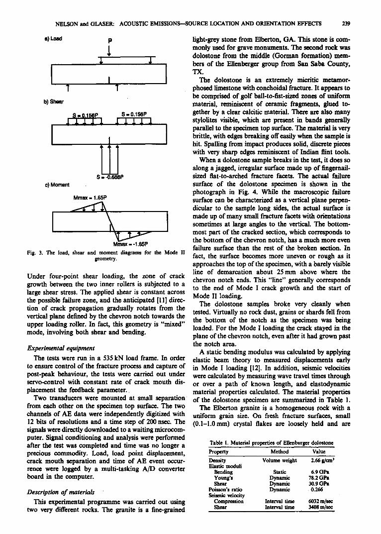
Figure 3 shows the shear and moment diagrams for Mode II loading derived from simple beam theory.

P

[ I

~) ~lo film - " ~ trdn Fig. 2. The predominantly shear geometry used for Mode II loading.

NELSON and GLASER: ACOUSTIC EMISSIONS--SOURCE LOCATION AND ORIENTATION EFFECTS 239

a) Load

"r

b) Shear

P 1

,t

I 1

S=Q156 P S =0.156P

c) Moment

Mmax = 1.65P

Mmax ,, -1.65P

Fig. 3. The load, shear and moment diagrams for the Mode II geometry.

Under four-point shear loading, the zone of crack growth between the two inner rollers is subjected to a large shear stress. The applied shear is constant across the possible failure zone, and the anticipated [11] direction of crack propagation gradually rotates from the vertical plane defined by the chevron notch towards the upper loading roller. In fact, this geometry is "mixed" mode, involving both shear and bending.

Experimental equipment The tests were run in a 535 kN load frame. In order

to ensure control of the fracture process and capture of post-peak behaviour, the tests were carried out under servo-control with constant rate of crack mouth displacement the feedback parameter.

Two transducers were mounted at small separation from each other on the specimen top surface. The two channels of AE data were independently digitized with 12 bits of re---olutions and a time step of 200 nsec. The signals were directly downloaded to a waiting microcom- puter. Signal conditioning and analysis were performed after the test was completed and time was no longer a prec ious c o m m o d i t y . L o a d , l oad po in t d isp lacement , crack mouth separation and time of AE event occur- rence were logged by a multi-tasking A/D converter board in the computer.

Description of materials This experimental programme was carried out using

two very different rocks. The granite is a fine-grained

light-grey stone from Elbenon, GA. This stone is com- monly used for grave monuments. The second rock was dolostone from the middle (Gorman formation) mem- bers of the Ellenberger group from San Saba County, TX.

The dolostone is an extremely micritic metamor- phosed limestone with conchoidal fracture. It appears to be comprised of golf ball-to-fist-sized zones of uniform material, reminiscent of ceramic fragments, glued to- gether by a clear calcitic material. There are also many stylolites visible, which are present in bands generally parallel to the specimen top surface. The material is very brittle, with edges breaking off easily when the sample is hit. Spalling from impact produces solid, discrete pieces with very sharp edges reminiscent of Indian flint tools.

When a dolostone sample breaks in the test, it does so along a jagged, irregular surface made up of fingernail- sized flat-to-arched fracture facets. The actual failure surface of the dolostone specimen is shown in the photograph in Fig. 4. While the macroscopic failure surface can be characterized as a vertical plane perpendicular to the sample long sides, the actual surface is made up of many small fracture facets with orientations sometimes at large angles to the vertical. The bottom- most part of the cracked section, which corresponds to the bottom of the chevron notch, has a much more even failure surface than the rest of the broken section. In fact, the surface becomes more uneven or rough as it approaches the top of the specimen, with a barely visible line of demarcation about 25 mm above where the chevron notch ends. This "line" generally corresponds to the end of Mode I crack growth and the start of Mode II loading.

The dolostnne samples broke very cleanly when tested. Virtually no rock dust, grains or shards fell from the bottom of the notch as the specimen was being loaded. For the Mode I loading the crack stayed in the plane of the chevron notch, even after it had grown past the notch area.

A static bending modulus was calculated by applying elastic beam theory to measured displacements early in Mode I loading [12]. In addition, seismic velocities were calculated by measuring wave travel times through or over a path of known length, and elastodynamic material properties calculated. The material properties of the dolostone specimen are summarized in Table 1.

The Elberton granite is a homogeneous rock with a uniform grain size. On fresh fracture surfaces, small (0.1-1.0mm) crystal flakes are loosely held and are

Table 1. Material properties of Ellenburger dolostone

Property Method Value

Density Volume weight 2.66 g/cm 3 Elastic moduli

Bending Static 6.9 GPa Young's Dynamic 78.2 GPa Shear Dynamic 30.9 GPa

Poisson's ratio Dynamic 0.266 Seismic velocity

Compression Interval time 6032 m/Nc Shear Interval time 3408 m/see

-i~~i.~ ~I~'

"i


Table 2. Material properties of Elberton granite

Property Method Value

Density Volume w~ght 2.60 g/Clll 3 Elastic moduli

Bending Static 5.7 GPa Young's Dynamic 35.6 GPa Shear Dynamic 14.2 GPa

Poisson's ratio Dynamic 0.253 Seismic velocity

Compression Interval time 4061 m/see Shear Interval time 2337 m/see

aligned parallel to the macroscopic failure plane. The granite fracture surface is smooth and with little relief, as is apparent in Fig. 5 which shows the granite specimen after failure. When loaded in Mode 11, the granite crack extended out of the Mode I plane, and the crack propagated towards the upper load point.

There was a noticeable amount of "flaky" detritus produced during the fracture process in the granite. During the test, this material rained from the new crack surfaces and accumulate below the specimen. When the fractured surface was examined, the crack surface was actually a damaged zone many millimetres deep perpendicular to the macroscopic failure plane. Loose flakes ranging up to 10 mm in size could be easily dislodged over the entire failure surface. This is in contrast to the dolostone which exhibited smooth, sharp failure plane facets, and a much thinner or more confined crack process zone of microfractured material.

The mechanical properties of the granite specimen were obtained in the same manner as those for the dolostone and are summarized in Table 2.

Acoustic emission transducers

Tests with conventional commercial AE transducers show that detected waveforms are as much a function of transducer response as of sample behaviour, therefore, commercial transducers are not suitable for a study involving actual surface displacement history [13-15]. In addition, commercial transducers respond to either displacement, velocity or acceleration, depending upon frequency [16]. This uncertainty about the measurement makes the concept of quantitative analysis of high- fidelity signal records difficult to apply to data from commercial detectors.

NIST-type high-fidelity piezoelectric displacement transducers were built and used throughout this experimental programme. The NIST transducer is fairly compact, easy to use, and has a small "footprint" to avoid an aperture effect for frequencies well over 1 MHz. The calibration work at NIST has shown this transducer to be a displacement-sensitive device with practically no sensitivity in the transverse direction. A large brass backing acts as a half-space to absorb the wave energy once it passes through the PZT-5 crystal, eliminating ringing [18].

The amplitude spectrum of the NIST transducer for a step pulse is constant within 2 dB to a frequency over 1 MHz. The phase spectrum is within 0.3 rad for the same frequency range [4, 17]. These transducers have

been extensively tested and proven in the large amount oftheoreticat work undertaken at NIST. This transducer has also been used in experiments carried out at Johns Hopkins University and has been found to give results which compare very well with measurements using a laser interferometer [18].

System calibration

The bias of a system--how a system changes information passing through it--can be characterized by the system's impulse response function. Inputting a perfect impulse function into the sample to determine the system impulse response function is an impossible task. There- fore, system bias was characterized by the readily- achievable and closely-related system step response function [4, 19]. Following standard AE practice [19, 20], a step-like pulse with a rise time of less than 0.5/~sec was input into the sample by breaking a very small-diameter glass capillary tube against the bottom of the sample. For the frequencies of interest and time durations in- volved, this stress drop can be considered a step impulse.

In order to remove the system bias from collected signals, a system inverse filter was obtained by decon- volving the digitized received calibration signal with the idealized input signal. Since the direct polynomial division method is unstable for virtually all real-life systems, the standard geophysical techniques of least-square time domain deconvolution were used [21, 22], and is presented in detail in the Appendix. Experimentation using the system step response as the idealized source yielded poor results. The least-square inverse filter acted as a low pass filter, rather than sharpening response and restoring the high-frequency components attenuated by the rock. A simple solution to this problem was to note that the derivative of the step impulse is the delta function. Taking the first derivative of the system step response gave the impulse response function of the entire system.

The use of the anti-aliasing filter means that a perfect spike, made up of all frequency components at equal amplitude, is not the proper choice for the deconvolution model. Therefore, the input impulse was modelled as a very narrow Gaussian window, shown in Fig. 6, with frequency response mimicking that of the digitizer's low pass filter. The signal actually calculated when this method was applied is the system impulse response function, which was very close to the Gaussian ideal without inverse filtering. This is especially true of the dolostone impulse response function which is pictured in Fig. 7. The system function is seen to be the same as the ideal with some trailing oscillations of small amplitude.

Since the actual and ideal impulse functions are so similar, the system obviously had very little effect on the input signal. Figure 8 presents a signal before (Fig. 8a) and after (Fig. 8b) the deconvolution process. Deconvo- lution here acts merely as a "sharpening" filter and does not change the macroscopic shape of the event. Since almost all signal energy was below 350 kHz, the general shape of the signals do not incorporate the higher frequencies that are boosted by deconvolution. However it is important to note that, for other lithologies and for

242 NELSON and (3LASER: ACOUSTIC EMISSIONS---SOURCE LOCATION AND ORIENTATION EFFECTS

O "o .2 "8. E <

.N_

#

Q

E <

N . w

o z

0 -

-I 0 -

- 2 0 - ].

0

-1

2 4 6 8 10 12 14 16

"1"]me (microsec) Fig. 6. Thc "ideal" impulse.

2 4 6 8 10 12 "time (micros)c)

Fig. 7. The impulse response function of the dolostone system.

14 16

real rock masses, material filtering may be very much more important.

At this point, all effects of the experimental setup arc accounted for. The large size of sample, and the fact that only the initial portion of recorded AE signal (unaffected by reflections and resonances from the specimen boundaries) is used, ensure that the specimen size and shape will not affect the recorded AE wavcforms. The calibration exercise ensures that the effect of the stress wave travelling through the specimen was accounted for. Investigation of the remaining systemic effects of source location and orientation relative to transducer are dis- cussed in the next section.

EFFECTS OF SOURCE LOCATION ON CRACK PLANE

In the broadest sense, the macroscopic failure surface of the specimen in this study can be described as a vertical plane. When the failure surface is examined on a finer scale, the surface is rough with facets oriented at various angles to the vertical. This surface roughness was

especially noticeable for dolostone specimens. Since transducer locations were fixed throughout a test, and the location of incremental crack growth varies over almost a 300 mm square, the events during the test sequence occur at systematically varying angles to the transducers. Therefore, the effect of the location of each event on the shape of the waveform recorded needs to be clarified. A parametric study to isolate these changes was launched under controlled conditions to isolate the possible effect of source location with respect to the transducers on signal shape, without any introduced effects from local surface morphology.

The test environment was modelled as a free saw-cut plane, perpendicular to the plane of transducer mounting. The transducers measure displacement strictly normal to the mounting face. The layout for this study is illustrated in Fig. 9, where the transducer locations are shown and the coordinate system for this study is introduced. The coordinate system origin is at the upper- left corner of the test face. The distance from the front face in the direction of the transducer is given by the X-coordinate, the distance across by the Y-coordinate,

> E

1 5 -

1 0 -

5 -

1 5 -

1 0 -

5 -

-5 "

-10-~ -15

ps ps Fig. 8. Comparison of a signal before (a) and after (b) deconvolution.

I I I I I I I I I I 0 10 20 30 40 0 10 20 30 40

NELSON and GLASER: ACOUSTIC EMISSIONS---SOURCE LOCATION AND ORIENTATION EFFECTS 243

A:X.leOmm e:X-2OOmm / . / ~ I t ~ / ' ~ ~ f " Yz:150mmmm Y.190mm / . / / I 10

~ ~ : : ~ 300 m / ~0 a ¢ ~ ® ~ n , n e event

300 mm I I I I I I 0 10 20 30 40 50

Fig. 9. Layout of location study.

and the vertical distance from the top surface by the Z-coordinate. The position and orientation of the transducers with respect to the test plane was identical to that used in actual test situations.

The test simulation of location effects proceeded with repeatable step impulses input on the vertical plane. This surface is analogous to the plane defined by the chevron notch in the actual specimen, and is congruent with the macroscopic failure plane. The step impulses were imparted against this surface, so the sense of action of the pulse was parallel to the top horizontal plane monitored by the two transducers. Any potential effect from the other (removed) half of the actual test specimen was ignored as was any localized influence of the crack tip and process zone. As a result of this model, signal travel paths in this parametric study of the effects of location closely resemble those used by the actual AE signals.

The glass capillary was used as a well-defined and repeatable source since a numerical study [23] suggests that the difference between a signal from a monopole source (capillary break on open surface) and a dipole (pure tensile crack) is very small. This choice is further supported by consideration of the nature of both the actual AE and capillary-break event mechanisms. When the glass capillary, lying fiat against the rock surface, is slowly loaded, the stress slowly builds up. When the glass suddenly breaks, there is a correspondingly sudden stress drop [4], giving a characteristic step pulse. Similarly, when the rock ligament is loaded in tension, the stress slowly builds until critical conditions for fracture propagation are reached, and the sudden crack extension releases the energy stored in the material.

A typical AE waveform and a rectified capillary break signal are presented in Fig. 10a and b. Although the signal amplitudes differ greatly, the shapes of the waveforms for the actual event and the glass capillary source are very similar, supporting a conclusion that the sources are extremely similar. Note that for the capillary signal zero displacement corresponds to the quasi-static application of load and the step-like surface displacement with the extremely sudden removal of load.

The arrivals of the compressional (P-wave), shear (S-wave) and Rayleigh waves (R-wave) is labelled in Fig. 10. The arrival of these wave modes were calculated

-200 -

- 1 O0 -

o

l°° t 200

S

b) capglap/signal 0 X-O ram, Y .115 ram, ; [ -90 mm

I I I I I I 0 10 20 30 40 50

R /

/ I 8O

Fig. 10. Comparison of a real AE event (a) and a signal from a breaking capillary (b).

since the distance from the source and transducer was known, as well as experimental mode velocities. In addition, the arrivals could be identified by comparing the shape of the waveforms to both theoretical and experimental results [24-26]. Since the source is essen- tially a point source far from the receiver, the vertical component of S-wave arrival will have a distinct polarity [4, 241.

The face upon which the capillaries were broken was a very smooth diamond-saw-cut surface. The geometry of the stressed ligament was inscribed on the face, and a grid of locations representative of the locations of actual events was laid out as illustrated in Fig. 11. Since the chevron notch ligament geometry is symmetric, the impulses were only input onto one side of the centreline.

The results from the four lines of impulse sources were much the same, with an increase in the effect of surface reflections for the locations nearer the sample side. Because of space constraints, only results of the centreline study will be examined in detail.

Centreline study

A series of events were input up the centreline, 150 mm from either side edge (Y - 150 mm). This allowed the effects of the bottom and top surfaces to be studied with a minimum of interference from reflections off the sample sides. One transducer was used, and the horizontal location of the transducer remained constant

244 NELSON and GLASER:

Y-O

z.o

Z.,40.-.)

Z=65-.)

Z,,90->

7.=115-

Z=140.

Z=165- I Z=I~->

Z,=215 --~

Z-,240-~

Z-270-~

ACOUSTIC EMISSIONS--SOURCE LOCATION AND ORIENTATION EFFECTS

(Note: all dhJtlmc~ In ram)

Y=40 Y-75 Y-115 Y -150

%%%%%%%% • S SS'

• SS** s A*

S

%'%%

%%%%'~ S %% **** "o"

Fig. 11. Location of input step impulses on the free rock face for the location effect study. Note: all Y and X coordinate dimensions are given in millimetres.

(X = 180 ram) as the vertical distance (Z) from source to transducer was varied from 240 to 40 ram. In order to simplify analysis and comparison of results to published findings, the locations are presented as a non-dimen- sional ratio of horizontal distance from the transducer to depth (X:Z). The X-value remains at 180 mm for all signals in this study. Figure 12 shows the waveforms obtained as the source varied over X f0 .75Z to X --- 4.5Z. The surface displacements are shown as signal amplitudes, normalized to the signal peak amplitude occurring over the first 50 #sec of signal.

All the events in Fig. 12 exhibit a very sharp, sudden displacement at the initial wave arrival, followed by a table-like plateau of sustained displacement. At later times a short increase in displacement occurs before the sudden displacement change associated with the arrival of the S-wave and then the R-wave [24, 25] energy. Note that the time lag between P- and S-wave arrivals dimin- ishes as the straight line travel path to the transducer becomes smaller, from 312 to 204 mm.

The event most distant from the transducers, at X = 0.75Z, shows the arrival of a definite reflection at

|

4 0 -

30

2 0

1 0 -

I I I I I 0 10 20 30 40 50

las

Fig. 12. Effects of vertical distance from tramducer A along the ligament centreline.

l

NELSON and GLASER: A C O U S T I C E M I S S I O N S - - S O U R C E LOCATION A N D O R I E N T A T I O N EFFECTS 245

about 22 #see. This is a reflection off the sample bottom, and occurs as surface movement in the direction opposite to the direct P-wave energy. There is then additional movement in the main P-wave direction from the reflection off the sample side, followed by a plateau, before the sudden arrival for the shear energy at about 45 p sec.

For the event at X - 0.95Z, the effects of the reflections off the bottom are no longer evident. The characteristic rise before the shear energy displacement becomes a pointed peak and less of a plateau due to the SP-wave (critically refracted S-wave) now arriving slightly before the shear energy. As the SP-wave arrives ever earlier for X = 2.05Z, the pre-S-wave peak again appears more plateau-like. There is a steady increase in the amount of "ramping" or gradual increase in the surface displacement following initial arrival as the angle between source and transducer flattens from X = 0.95Z to 1.25Z, and the reflection off the bottom arrives much later, after the large shear displacement. These results are identical to those reported by Cooper et al. [26] using a laser interferometer, which measures absolute normal surface displacement.

Figure 13 shows the waveform from the event at X=0.95Z, and the arrivals of reflections, S- and SP-waves are identified. For comparison, Fig. 14 shows the waveform from the event at X = 1.6Z. The arrival of reflections from the sample side and bottom are labelled, as is the SP-wave arrival. Since the locations of source and receivers were known, the time delays between arrivals for these simple cases were calculated using the measured wave velocities. Note how the change in relative time of arrival between the side reflection and SP-wave changes the shape of the short increase in displacement before the S-wave arrival.

For events nearing the sample top, at X = 2.05Z, the displacements again exhibit a plateau immediately after the initial P-wave arrival due to the SP-wave arriving earlier with respect to the P-wave. However, there is no real change in the macroscopic shapes of the signals until the shear arrival, and the waveforms can all be characterized as approximating a "box-car" in shape.

The greatest effect of location is possibly shown by Fig. 15, which shows the event at X = 4.5Z, 40 mm from the top of the sample. Note that there is a ramp-like

-10

100

200 1

300 I I I I I 0 10 20 30 40

gs

Fig. 14. Waveform from the centreline event at X -- 0.95Z.

change in direction of the surface deflection 12/z sec after signal arrival (seen after the SP arrival) in a sense opposite to the initial P-wave motion, followed by another sharp reversal of motion at 26 #sec thought to be due to the arrival of the reflection off the specimen side. The shear wave arrives at 29psec (based on calculations) in the direction opposite to the initial P-wave motion.

For all events very close to the top (X > 3.6Z) there is a "sloping" direction change which might be due to an early arrival of additional interference due to the close proximity of the specimen comer. It can be argued that this comer does not exist in the actual test specimen since the ligament is intact above the crack front, but it will be seen that this signal shape was detected towards the end of actual tests. Alternatively, this characteristic shape may be due to the morphology of the P- and S-wave radiation patterns. The observation that the S-wave arrives in the direction opposite the initial P-wave arrival is supported by work of other researchers [26].

Off-centreline effects

The effect of horizontal location can best be summarized by examining the changes in signal shape due to changes in the Y-direction alone. Figure 16 shows the results from a step force input at a constant depth (X = 2.05Z), and the horizontal distance from source to transducer varying from Y = 40 to 150 mm. The effect of

-15o-] Bottom

'°°1

100

1 5 0 z i t i I 0 10 20 30

p=

Fig. 13. Waveform from the centreline event at X = 1.6Z.

I

40

-200 -

- 1 0 0 -

0 -

100 -

200

$

~ n i l l i H i i l m i l 0 10 20 30

ps

Fig. 15. Waveform from the centreline event at X = 4.5Z.

40


3o ~"

i5 20, I 8 v ' v

°" / __..vL.,q .-

:,,o_ :of -y k>g 5 -

I I I I I 10 20 30 40 50

p.s

Fig. 16. Effects of horizontal distance from transducer A at depth X = 2.05Z.

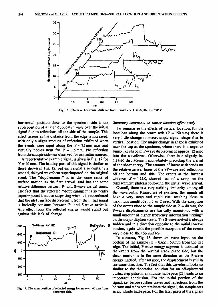
horizontal position close to the specimen side is the superposition of a late "duplicate" wave over the initial signal due to reflections off the side of the sample. This effect lessens as the distance from the edge is increased, with only a slight amount of reflection exhibited when the events were input along the Y--75 mm axis and virtually non-existent for ¥ ffi 115 ram. No reflection from the sample side was observed for centreline sources.

A representative example signal is given in Fig. 17 for g = 40 ram. The leading part of this signal is similar to those shown in Fig. 12, but each signal also contains a second, delayed waveform superimposed on the original event. The "doppleganger" is in the same sense of surface motion as the first arrival, and has the same relative difference between P- and S-wave arrival times. The fact that the reflected "doppleganger" is so neatly superimposed is not so surprising when it is remembered that the ideal surface displacement from the initial signal is basically constant between P- and S-wave arrivals. Any effect from the reflected energy would stand out against this lack of change.

-300 -

-200 -

-100 -

0

100 -

2 0 0 -

300

Yg4Omm X~l .6Z Reflected S

I I I I I I 0 10 20 30 40 50

ps

Fig. 17. The superposition of reflected energy for an event 40 nun from specimen side.

Summary comments on source location effect study

To summarize the effects of vertical location, for the locations along the centre axis (Y--150 mm) there is very little change in macroscopic signal shape due to vertical location. The major change in shape is exhibited near the top at the specimen, where there is a negative ramp-like shape in P-wave displacement approx. 12 ~ sec into the waveforms. Otherwise, there is a slightly increased displacement immediately preceding the arrival of the shear energy. The amount of increase depends on the relative arrival times of the SP-wave and reflections off the bottom and side. The events at the furthest distance, X =0.75Z, showed less of a ramp on the displacement plateau following the initial wave arrival.

Overall, there is a very striking similarity among all the waveforms. Regardless of position, the signals all have a very steep and rapid rise, reaching close to maximum amplitude in 1 or 2/~ sec. With the exception of the events close to the sample side at Y = 40 rnm, the P-wave displacements are basically monotonic with a small amount of higher frequency information "riding" on the major displacements. The S-wave arrival is always sudden and in a direction opposite to the initial P-wave motion, again with the possible exception of the events very close to the top surface.

In contrast, Fig. 18 shows an event input on the bottom of the sample (X = 0.6Z), 50 mm from the left edge. The initial, P-wave energy segment is identical to the events from the vertical crack plane side, but the shear motion is in the same direction as the P-wave energy. Indeed, after 60/~sec, the displacement is still in the same direction. The fact that this waveform looks so similar to the theoretical solution for an off-epicentral buried step pulse in an infinite half-space [27] leads to an important conclusion. For the initial portion of the signal, i.e. before surface waves and reflections from the bottom and sides contaminate the signal, the sample acts as an infinite half-space. For the later parts of the signals


-20 -1

- 1 0 -

O -

1 0 -

20

Y = ~ m X:0.6Z (on sample u n d e r s i d e )

I I I I I I I 0 10 20 30 40 50 60

Fig. 18. Surface displacement due to a step impulse input on the underside of the sample.

Table 3. Location and orientation of representative fracture facets

E ~ t Y -, Z ~ Azimuth Dip position (ram) (ram) X : Z (horizontal*) (vertical °)

A 127 135 1.3 - 18 42 B 200 114 1.6 33 20 C 137 58 3.1 - 1 5 - 2 3 D 137 53 3.4 - 18 52 E 155 58 3.1 - 3 5 50 F 155 97 1.9 - 3 0 - 3 0 G 142 206 0.9 - 34 - 22 H 58 160 1.1 - 1 8 54 J 97 168 1.1 8 - 4 3 K 15 69 2.6 - 4 0 18 L 43 53 3.4 28 - 2 7 M 277 71 2.5 5 26 N 282 132 1.4 - 2 0 - 13 O 3O2 99 1.8 - 6 6 P 292 168 1.1 4 31 Q 262 170 l.l 11 39

in this study, the effects of the reflections from the sample sides and bottom do not affect the overall shape of the waveform. This further supports the decision to accept the results from this parametric model. For the initial P-wave displacements, the location of the signal source (vertical or horizontal) has little effect. This could be expected from the P-wave radiation pattern for a non-point dipole or tensile crack, which resembles a "peanut" of figure "8" in shape. For this case, all displacements are in the same direction, regardless of location relative to the source.

EFFECTS OF CRACK INCREMENT FACET ORIENTATION

While the macroscopic failure plane is analogous to the vertical plane shown in Fig. 9, and is perpendicular to the specimen top surface, the actual crack increments grow on small surfaces, or facets, at sometimes large angles to the macroscopic failure plane. Since the orientation and direction of movement of the source event in relation to the receiver can have a large effect on the waveforms due to the unique geometric relation of each to the source plane [27-30], this effect must be examined. Again, an experimental approach will be taken, with the effects due solely to geometric location known and

~meth -

~T

,,q I

s

s S s

s

Azimuth - negative olp - posmve

I~ - ne~tve Dip - n ~ e

Fig. 19. Def~tion of the normal vectors defining the fracture facets.

RMMS 29/3--E

accounted for. All events in this study were applied to facets on real crack faces.

The complexity and irregularity of the failure surface of the dolostone specimen is shown in Fig. 4, with the sample obliquely illuminated to highlight the fracture surface facets. In order to describe the orientation of the individual crack growth facets, the coordinate system defined in Fig. 19 was adopted. The orientation of each tested facet is described with dip and azimuth. The dip gives the angle of the facet to the horizontal, with 0 ° dip being a vertical plane with a horizontally applied input pulse. A plane has a positive dip if the normal to the facet has a component in the downward direction, away from the horizontal top of the sample. The azimuth is the bearing of the normal to the plane in the horizontal. Azimuth angles are given as positive if the normal points to the right (clockwise) of the specimen central axis. An azimuth of 0 ° indicates the facet surface is in the Y - Z plane.

Table 3 gives the Y (horizontal) and Z (vertical) location, and the azimuth and dip for each event in this study, with alphabetical event labels from A to Q. To put these events and locations into perspective, a schematic summary of the test locations on which the capillaries were broken is given in Fig. 20.

Experimental results on source orientation

Figures 21a-c show a representative sampling of one group of events, identified by their event label. The three events are shown in order of decreasing dip orientation, E, P and O. These are all ramp-like waveforms caused by a step-like source mechanism. From Table 3 it is seen that these events all resulted from capillaries broken on a fracture facet with a dip positive from horizontal. The locations of these events are well distributed, as is the fracture plane azimuth, leaving dip as the only relevant variable.

The question becomes at what dip angle does the step source cause a ramp-like displacement rather than the step-like motion observed in the centreline study. Some idea of the amount of positive dip needed to lose the sharp step-like rise is gained by looking at the waveform

248 NELSON and GLASER: ACOUSTIC EMISSIONS---SOURCE LOCATION AND ORIENTATION EFFECTS

i > y Z

• L D K E 0 8 C M

A

F

B

N H • J

• O O s

%%~% G J J ~ % % s s S

s s

s s

%~vs S

Fig. 20. Location of input of step impulses for the orientation effect study.

from location O in Fig. 21c. All the other listed source facets had a dip greater than 18 ° and the signals show a strongly ramp-like shape. Location O was on a surface with a dip of 6 ° and the signal exhibits a rise rate bridging the step-like and ramp-like waveform shapes.

One possible explanation for the event O signal shape is that the plane is close to the sample edge, producing interactions which smear the initial arrival and the side reflection. However, this is unlikely since the waveform has such a smooth shape and shows no obvious reflection arrivals. The more likely explanation of the longer rise time is the effect of the small (6 ° ) positive dip. This leads to the conclusion that, for fracture growth planes with a positive dip, the radiation pattern of the relevant source---crack or capillary break--is such that there is no sudden, large arrival of P-wave displacement.

Two exemplary signals from the remainder of the events from the orientation study are presented in Fig. 22a and b. For these events, the dip of the failure facets is negative and they all have the sharp, step-like initial motion that was exhibited in the location study. However, there are differences in the waveform after approximately the first 20 gsec, differences which cannot always be explained by location. The event in Fig. 22a closely resembles the event input into the underside of the block. The event in Fig. 22a has a dip of - 4 3 °, so that the source is orienting a large portion of its energy in the vertical direction towards the top, monitored, surface. For this event, the shear energy arrival is in the same direction as the P-energy motion. The event in Fig. 22b with a dip of - 3 0 ° also behaves in the same manner.

The effect of azimuth orientation is not so evident. The large ( - 4 0 °) rotation of the event K facet (shown in Fig. 23) towards the side only 15 mm away, combined with the positive dip, might be the cause of the energy so concentrated at the late end of the wave. The side

-100 - ,,) PoMion E : Dip,-S0 °, Azimuth--35 °

-50 - -

50

100

i

I I I I I 0 10 20 30 40

-150 -

-100 -

-50 -

o

5O

IO0

150

b) Position P : Dip,-31°, Az.irnuth-4 °

I I I I I 0 10 20 30 40

"200 t

-100

E 0

1°° t 2 0 O I

0

o) Podtion O : Dil>,,6 °, Azimuths.6 °

! I ! I 10 20 30 40

I.m

Fig. 21. Signals from breaking capillaries on surfaces with positive dip.

reflections could well be the main carrier of detected energy.

The location E facet also has a large ( - 2 5 °) azimuth. As shown by the signal in Fig. 24, it also has a similar, but much more angular, shape as the event from location K shown in Fig. 23. The location E is far from a side, and has a large + 50 ° dip so the SP-wave arrival becomes dominant. This example leads to the conclusion that the dip of the facet where an event originates is a more important parameter than the proximity of the side for diminishing the effect of the initial P-wave arrival.

Summary comments on roughness effects

The results of the location study provide a basis to understand fully the effects of the surface relative orientations on the wave shapes. For the events input onto the steeply-inclined fracture facets, there is a shift in energy


-400 -

- 2 0 0 -

2OO

4OO

• : ' " , ' - 1 0 0 -

~ -5o -

1 0 0

I I I I I I

0 10 20 30 40 5 0

gs

5 0 -

Dip : 50 °, Azimuth :

I I I | I I 0 10 2 0 3 0 4 0

Fig. 24. Waveform from the event at location E.

- 2 0 0 -

- 1 0 0 -

1 0 0

2 0 0

b) Posi t ion F : Dipff i-30", Azimuthf f i -30 °

I I I I I I 0 10 20 3 0 4 0 5 0

ps Fig. 22. Signals from breaking capillaries on surfaces with negative dip.

concentration towards the latter part of the wave when reflections and SP and shear energy begin to arrive. This is not true for the events input on the saw-cut surface perpendicular to the transducer plane, leading to the conclusion that the initial parts of the waveforms under study are very sensitive to the orientation of the source relative to the receiver.

A more concise conclusion can be made concerning the cause of the ramp-like rise of some events. This ramp-like rise is always associated with a positively dipping facet, where the direction of loading has some downward component away from the top free surface. The early part of the actual failure surface created by the Mode I loading of the dolostone is very flat compared

- 1 5 0 -

-1 O0 -

- 50 -

o

5 0 -

100 -

150

D i p : 1 8 °, A z i m u t h :

t, 0 1 0 2 0 3 0 4 0

lJS Fig. 23. Waveform from the event at location K.

to the latter portions, and should have produced few ramp-like AE events. The mid- to latter-part of this loading produced some large positive-dipping fracture facets, and a correspondingly increased number of ramp-like events.

A numerical study by Ohtsu and Ono [29] offers some theoretical basis for the effect of facet dip. They modelled three situations for facet dip = 0 °, + 20 ° and - 2 0 ° with a source function mimicking a capillary break. The simulated received waveforms were then deconvolved back to the source function. The source with positive dip orientation yields a ramp-like waveform. It is seen that a common step-like source results in different waveforms after proper signal processing, and these differences cannot be understood if facet dip is not taken into account.

Ohira and Pao [30] ran a series of tests on well-instru- mented compact tension steel specimens. They found two types of AE signals, shown in Fig. 25. The Type I signal is step-like in shape and was believed to occur at a very small angle to the macroscopic failure plane. The Type II signal is ramp-like and occurred with a large angle to the failure plane.

CONCLUSIONS

This parametric study shows that a wide range of surface displacement waveform shapes can result from a common source mechanism. These signals are recreatible by inputting the same step-like source pulse, which closely resembles a tensile crack growth increment, over variously oriented and located facets existing on the actual crack surface.

The effects of source orientation must be taken into account to ensure an insightful waveform classification process. The same step-like source function can appear as several different signals at variously oriented transducers, as is summarized in Fig. 26. Input on a vertical plane, this source causes a step-like displacement at the transducer monitoring the horizontal surface, with the S-wave arriving in the direction counter to the initial P-wave arrival. A ramp-like signal was caused by a step-like source mechanism acting in an orientation having a positive dip. This same mechanism acting on a plane with a negative dip yielded a step-like signal with


2.OOl- S( t ) Type I I

100 -~

S('t:) Type I

/ I

2.00

At: _a

1.oo

I I I / ] I I I I 0.5 1.0 1.5 2.0 0 0,5 t .0 1.5 2.0

Time (psec) Fig. 25. Effect of source facet orientation on the deconvoluted source signal from a compact tension steel specimen [30].

AT ~AMPI~ TOP SURFACE

. . . . . . . . . . . .

po,mm t~p

._1

Fig. 26. Simplified summary of effects of step-like source orientation on displacement of specimen top surface.

the S-wave arriving in the same direction as the initial P-wave arrival.

This study indicates a completely calibrated AE detection system has been developed, capable of faith- fully capturing and recording AE produced by fracture propagation through rock specimens. The effects of specimen and crack surface geometry are understood and can be accounted for. It now remains to use this system to capture and classify waveforms produced during crack propagation in rock. The results of such an experimental study are presented in a companion p a p e r [1 ].

Acknowledgements--This project is funded by the State of Texas Advanced Research Program, FICE Code 003658-512. Previous support was also provided by the National Science Foundation, Contract MSM-8600567. This support is greatly appreciated.

Accepted for publication 9 December 1991.

REFERENCES

1. Ghuter S. D. and Nelson P. P. Acoustic emmions produced by discrete fracture in rock--Part 2. Kinsmatia of crack growth during controlled Mode I and Mode H loading of rock. Int. J. Rock Mech. Min. Sci. & Geomech. Abstr. 29, 253-265 (1992).

2. Simmons J. A. and Clough R. B. Theory of aconstic emiuion, Proc. Int. Conf Dislocation Modelling Phys. Sys., pp. 464-497. Pergamon Press, Oxford (1981).

3. Evans A. G. and IAnzer M. Acoustic emission in brittle materials. Annual Rev. Mater ScL 7, 179-208 (1977).

4. Eitzen D. G., Breckenridge F. R., Clough R. B., Fuller E. R., I-hu N. N. and Simmons J. A. Fundamental developments for qmmti- tative acoustic emimon measurements. Interim Rept NP-2089, Prepared for Electric Power ~ h Institute (1981).

5. Sondergeld C. H., Estey L. H., Halleck P. M., Dey T. N. and Blacic J. D. Monitoring of acoustic emissions during the uniaxial deformation of large mJnples. Proc. 3rd Conf on Acoust. Emission / Microseismic Activity Geol. Structures Mater., pp. 147-158. Tram Tech, Clausthal, Fed. Rep. Germany (1984a).

6. Sondergeld C. H., Granryd L. A. and Estey L. H. Acoustic emissions during compression testing of rock. Proc. 3rd Conf Acoust. Emi~sion/Mieroseismic Activity Geol. Structures Mater., pp. 131-145. Trans Tech, Clansthal, Fed. Rep. Germany (1984b).

7. Sondergeld C. H. Desirable sample dimensions for detailed acoustic emi~on studies. Geophys. Res. Lett. 8, 695-697 (1981).

8. Ingraffea A. R. Mixed-mode fracture initiation in Indiana limestone and Westerly granite. Proc. 23ut U.S. Syrup. Rock Mech., pp. 186-191 (1981).

9, Carpentieri A., Ferrara G. and Melchiorri G. Single notched specimen subjected to four point shear, an experimental investigation. Fracture of Concrete and Rock: Recent Developments, pp. 605-614. Elsevier Applied Science, Essex, U.K. (1989).

10. Jenq Y. S. and Shah S. P. Trajectory and stability of cracks in concrete subjected to mixed mode loading. Proc. 1989 SEM Spring Conf Exp. Mech., pp. 43-50. Soc. Experimental Mech., Bethni, CT (1989).

11. Fergnson P. M. Reinforced Concrete Fundamentals, pp. 106-107. Wiley, New York (1979).

12. Lama R. D. and Vutukuri V. S. Handbook on Mechanical Proper- ties of Rock, VoL II, pp. 46-51. Trans-Tech, Clansthal, Fed. Rep. Germany (1978).

13. Pao Y.-H. Theory of acoustic emmion. Elastic Waves and Non- destructive Testing of Materials, AMD, Vol. 29, pp. 85-106. ASME, NY (1978).

14. Hso N. N. and Hardy S. C. Experiments in acoustic emission waveform analysis for characterization of AE sources, sensors and structures. Elastic Waves and Nondestructive Testing of Materials, AMD, Vol. 29, pp. 85-106. ASME, NY (1978).

15. Glaser S. D. System effects of AE wave, forms from known sources. Prac. Fifth Conf on Acoustic Emi~sion/Microseismie Activity in Geologic Structures and Mater. In press, The Pennsylvania State Univer~ty (1992).

16. Shibata M. A theoreticatl evaluation of aconstic emi~on the rise time effect of dynamic forces. Mater. Evaluat. 42, 107-120 (1984)o

17. Proctor T. M, Jr, Breckeuridge F. R. and Eit;mn D. G. The development of high fidelity acoustic emission tramducers. NDE in the Nuclear Industry, 6¢h Int. Conf., pp. 329-337 (1983a).

18. Glass J. T. and Green R. E. Jr. Aconstic enfimon during defor- marion and fracture of three naval alloy steels. Mater Famhwt. 43, 864-872 (1985).

19. Beatti¢ A. G. Acomtic emimon, principles and in~mmentation. J. Aeoust. Em~. 2, 95-128 (1983).

20. Breckenridge F. It., Proctor T. M., Hsu N. N., Fick S. E. and Eitzen D. G. Transient sources for acoustic emission work. Prac. lOth Int. Acoust. Emission Syrup., NDI Japan, pp. 20-37 (1990).


21. Menke W. Geophysical Data Analysis: Discrete Inverse Theory. Academic Press, Orlando, FL (1984).

22. Silvia M. T. and Robinson E. A. Decon~lution of C~ophysical Time Series in the Exploration for Oil and Natural Gas. Elsevier, Amsterdam (1979).

23. Aizawa T., Kishi T. and Mudry F. Acoustic emission wave characterization: a numerical simulation of the experiments on cracked and uncracked specimens. J. Acoust. Emiss. 6, 85-92 (1987).

24. Pekeris C. L. and Lifson H. Motion of the surface of a uniform elastic half-space produced by a buried pulse. J. Acoust. Soc. Am. 29, 1233-1238 (1957).

25. Scruby C. D. Quantitative acoustic emission techniques. Nondest. Testing, Vol. 8 (Sharpe R. S., Ed.), pp. 141-210. Academic Press, London (1985).

26. Cooper J. A., Crosbie R. A., Dewhurst R. J., McKie A. D. W. and Palmer S. B. Surface acoustic wave interactions with cracks and slots: A noncontacting study using lasers. IEEE Trans UltraSon. UFFC-33, 462-470 (1986).

27. Ohtsu M. Mathematical Theory of Acoustic Emission and its Application, VoL XXXII, pp. 1-28. Mere. Faculty Engineering Kumamoto University (1987).

28. Hayashi K. and Nishimura H. Considerations on field AE data based on theoretical studies of elastic waves due to sudden movement of a subsurface reservoir crack. Proc. 8th Int. Acoust. Emission Syrup., NDI, Japan, pp. 742-749. (1986).

29. Ohtsu M. and Ono K. The generalized theory and source represen- tations of acoustic emission. ?. Acoust. Emiss. 5, 124-133 (1986).

30. Ohira T. and Pao Y.-H. Quantitative characterization of micro- cracking in A533B steel by acoustic emission. Met. Trans. A 20A, 1105-I114 (1989).

31. Braceweli R. N. The Fourier Transform and its Applications, pp. 24-48. McGraw-Hill, NY (1978).

32. Robinson E. A. and Treitel S. Geophysical Signal Analysis. Prentice-Hall, Engiewood Cliffs, NJ (1980).

33. Strang G. Linear Algebra and its Applications. Academic Press, Orlando, FL (1980).

A P P E N D I X A

Least-Squares Deconvolution Assuming a linear elastic body and a transient signal that is

stationary and ergodic, the effect of a waveform travelling through a body can be understood as a filtering process. This is shown pictorially in Fig. A1. The effect of this filtering can be expressed mathematically as convolution [21, 31], which is written:

rt ffi X,* Ft (AI)

where Yt is the detected or resulting signal, X t is the original or input signal and F t is the modifying or filter function.

In discrete form, convolution is represented by the formula:

Y, ffi ~ X,F~ _,. (A2) l

¢ ~ 0

Equation (A2) can be understood as the process of polynomial, or serial, multiplication [31]. In this interpretation, each element of t ic time series is taken as the coefficient of an n-length polynomial (or coefficients of the Z-transform [31]). Serial multiplication can also be written in matrix form as follows:

Yo

Yt

.Y,+~- I

"fo f,

= =

f , - ]

0

0

0 0 0 0

A o o o

A fo o o

A fo o

f , - , A fo

0 f._, f,

0 " X 0

0

0 Xm - I

0 0

0 0

fo. 0

(A3)

xt (input ~gn~; .~ R (,Rot) I >Yt (output ~gn~)

Fig. A 1. Pictorial representation of the filtering effect of a waveform passing through an elastic body.

Where n is the number of elements in the filter vector and m is the length of the input time series.

Equation (A3) can be written in shorthand as:

y ffi Fx. (A4)

Deeonvolution is the inverse of convolution. The deconvolution operator can be e x p r - ~ as

x -- F- I y, (A5)

where F- I is the function which removes the biasing effect of the system from the detected waveform, yielding the original source signal.

In this study deconvolution is used to calculate the system inverse filter. In this case the ori~nal signal input into the body is known, as is the affected signal which is the output of the detection system. In reference to equation (AI), Xt and Yt are known and the filter Ft is the unknown. The most straightforward method to evaluate F t is direct polynomial division [31]. Unfortunately, for real signals which incorporate noise, direct polynomial division does not yield usable results since there will be a large error when the irrational result of the division has to be arbitrarily truncated. The data known are not "exact" or infinite in length [21]. In addition, there can be more than one filter that can transform the given input into the detected output [32].

The common solution to this problem is to calculate an inverse fiter g that transforms the input into some output d such that the square of the error between the actual output y and the calculated output d is minimum. From linear algebra [32,33] it is found that the solution to this problem is:

Ig ---- [FTF] -] FTX, (A6)

which are known as the normal equations. In matrix notation the normal equations are:

w0

Wl

wn_t

r 0 r I

r t r 0 r]

r t r 0 r,

rt r0 rt

rt ro

n,_t • rl

rn-t go 1 g!

ro g, ,

(AT)

here ri, gi and wi, i = 0, 1, 2, 3 . . . . . n - 1 are the autocorrelation of the measured waveform y, the inverse filter g and crosscorrelation of the measured output waveform with input signals y and x, respectively [22, 32].

The autocorrelation matrix is of a symmetric form called a Toepfitz matrix which is solved using Levinson recursion [22, 32]. The recursion algorithm is very efficient and allows the equations to be solved with only three n-length vectors in memory. The destabilizing effects of noise from digitization and truncation error is reduced by weighting of the zero lag of the autocorrelation.

The resulting inverse filter g when convolved with a waveform that has passed through the system, removes the system response from the recorded waveforms.

acoustic emissions produced by discrete fracture in rockglaser.berkeley.edu/glaserdrupal/pdf/ijrm 1...

Documents