acoustic maritime rapid environmental assessment during ...w3.ualg.pt/~sjesus/pubs/b21.pdf ·...

CINTAL - Centro de Investigacao Tecnologica do Algarve

Universidade do Algarve

Acoustic Maritime Rapid Environmental

Assessment during the MREA’04 Sea Trial

S.M. Jesus, C. Soares, P. Felisberto, A. Silva,

L. Farinha and C. Martins

Rep 02/05 - SiPLAB21/Mar/2005

University of Algarve tel: +351-289800131Campus da Penha fax: +351-2898642588005-139, Faro [email protected] www.ualg.pt/cintal

Work requested by CINTALUniversidade do Algarve, Campus da Penha,8005-139 Faro, Portugaltel: +351-289800131, fax: [email protected], www.ualg.pt/cintal

Laboratory performing SiPLAB - Signal Processing Laboratorythe work Universidade do Algarve, FCT, Campus de Gambelas,

8005-139 Faro, Portugaltel: +351-289800949, fax: [email protected], www.ualg.pt/siplab

Projects project NUACE (FCT) - POSI/CPS/47824/2002 andAOB - REA JRP and HFi JRP

Title Acoustic Rapid Environmental Assessment during theMREA’04 Sea Trial

Authors S.M.Jesus, C.Soares, P.Felisberto, A.Silva, L. Farinhaand C.Martins

Date March 21, 2005Reference 02/05 - SiPLABNumber of pages 40 (fourty )Abstract This report describes the data acquired with the

Acoustic Oceanographic Buoy (AOB) during the MREA’04sea trial, that took place aboard the R/V ALLIANCEfrom 29 March - 19 April 2004, in the vicinity ofSetubal, 50 km south from Lisboa, Portugal.

Clearance level UNCLASSIFIEDDistribution list NURC (1+DVD), ULB (1+DVD), RNLNC(1)

SiPLAB(1+DVD), CINTAL (1)Total number of copies 5 (five)

Copyright Cintal@2005

Approved for publication

E. Alte da Veiga

President Administration Board

III

Foreword and Acknowledgment

This report presents recent developments on the AOB system and the results obtainedduring its testing in the MREA’04 sea trial. The MREA’04 sea trial took place off thePortuguese coast, approximately 50 km south from Lisbon, in the period 29 March - 19April, 2004.

The authors of this report would like to thank:

• the NATO Undersea Research Centre for the opportunity for participating in thesea trial

• the scientist in charge Dr. Emanuel Coelho

• the collaboration of Saclantcen personnel

• the master and crew of the R/V Alliance

• the contribution of Prof. J.-P. Hermand and Mathias Meyer from ULB for theassistance, contribution and thoughtfull discussions.

• FCT (Portugal) for the funding provided under project NUACE (POSI/CPS/47824/2002).

IV

intentionally blank

Contents

List of Figures VII

1 Introduction 11

2 The Acoustic Oceanographic Buoy 132.1 AOB hardware . . . . . . . . . . . . . . . . . . . . . . . . . . . . . . . . . 132.2 AOB software . . . . . . . . . . . . . . . . . . . . . . . . . . . . . . . . . . 14

3 The MREA’04 sea trial 163.1 Generalities and sea trial area . . . . . . . . . . . . . . . . . . . . . . . . . 163.2 Ground truth measurements . . . . . . . . . . . . . . . . . . . . . . . . . . 173.3 Deployment geometries . . . . . . . . . . . . . . . . . . . . . . . . . . . . . 17

4 Acoustic data 224.1 Emitted signals . . . . . . . . . . . . . . . . . . . . . . . . . . . . . . . . . 22

4.1.1 Acoustic sources . . . . . . . . . . . . . . . . . . . . . . . . . . . . 224.1.2 Emitted signals for Acoustic REA . . . . . . . . . . . . . . . . . . . 234.1.3 Emitted signals for bottom inversion . . . . . . . . . . . . . . . . . 234.1.4 Emitted signals for underwater communications . . . . . . . . . . . 24

4.2 Received signals . . . . . . . . . . . . . . . . . . . . . . . . . . . . . . . . . 264.2.1 Received signals for acoustic REA and bottom inversion . . . . . . 264.2.2 Received signals for underwater communications . . . . . . . . . . . 26

4.3 Channel variability . . . . . . . . . . . . . . . . . . . . . . . . . . . . . . . 274.4 Underwater communications . . . . . . . . . . . . . . . . . . . . . . . . . . 29

5 Conclusions and future developments 32

A Hydrophone characteristics 34

B Thermistor chain main charateristics 37

C MREA’04 DVD-ROM list 38

V

VI CONTENTS

intentionally blank

List of Figures

2.1 Acoustic Oceanographic Buoy - version 1: block scheme. . . . . . . . . . . . 13

2.2 AOB control and monitoring software screeshots: area map with AOB lo-calization (a) and acoustic data monitoring (b). . . . . . . . . . . . . . . . 14

3.1 Maritime Rapid Environmental Assessment 2004 work area: global modelarea (blue) and target area (green) (a) and detailed map of the acousticactivity area (b). . . . . . . . . . . . . . . . . . . . . . . . . . . . . . . . . 16

3.2 Recorded CTD locations during days 7 to 10 April. . . . . . . . . . . . . . 17

3.3 recorded CTD profiles during days 7 to 10 April: temperature (a), soundvelocity (b) and first two EOF’s (c). . . . . . . . . . . . . . . . . . . . . . . 18

3.4 GPS estimated AOB and source ship navigation during the deployment onApril 7 at 12:09 UTC by 38.3096N-009.0205W with bathymetry map (a),estimated source range (b) and source depth (c). . . . . . . . . . . . . . . . 18

3.5 GPS estimated AOB and source ship navigation during the deployment onApril 8 at 12:26 UTC by 38.3532N-008.9989W with bathymetry map (a),estimated source range (b) and source depth (c). . . . . . . . . . . . . . . . 19

3.6 GPS estimated AOB and source ship navigation during the deployment onApril 9 at 11:35 GMT by 38.3743N-009.0047W with bathymetry map (a),estimated source range (b) and source depth (c). . . . . . . . . . . . . . . . 19

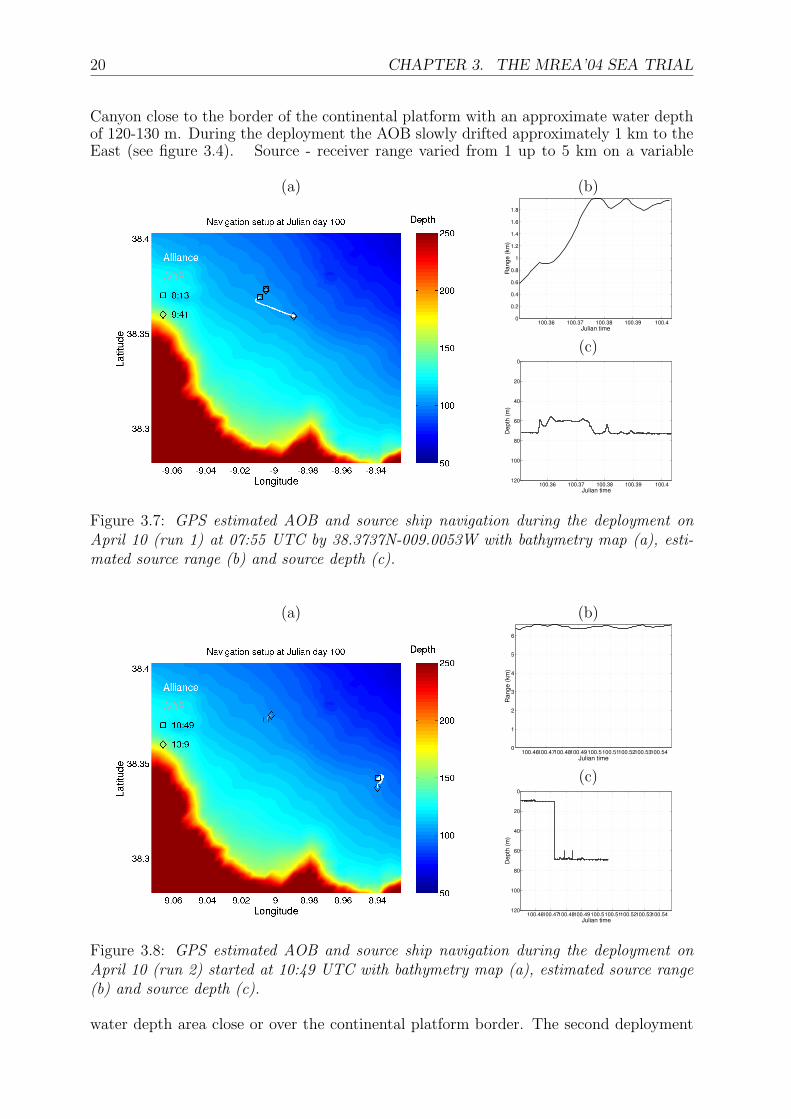
3.7 GPS estimated AOB and source ship navigation during the deployment onApril 10 (run 1) at 07:55 UTC by 38.3737N-009.0053W with bathymetrymap (a), estimated source range (b) and source depth (c). . . . . . . . . . . 20

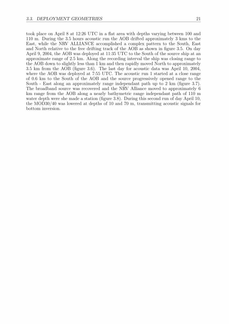
3.8 GPS estimated AOB and source ship navigation during the deployment onApril 10 (run 2) started at 10:49 UTC with bathymetry map (a), estimatedsource range (b) and source depth (c). . . . . . . . . . . . . . . . . . . . . . 20

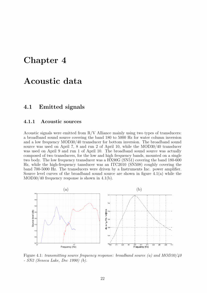
4.1 transmitting source frequency response: broadband source (a) and MOD30/40- SN2 (Seneca Lake, Dec 1990) (b). . . . . . . . . . . . . . . . . . . . . . . 22

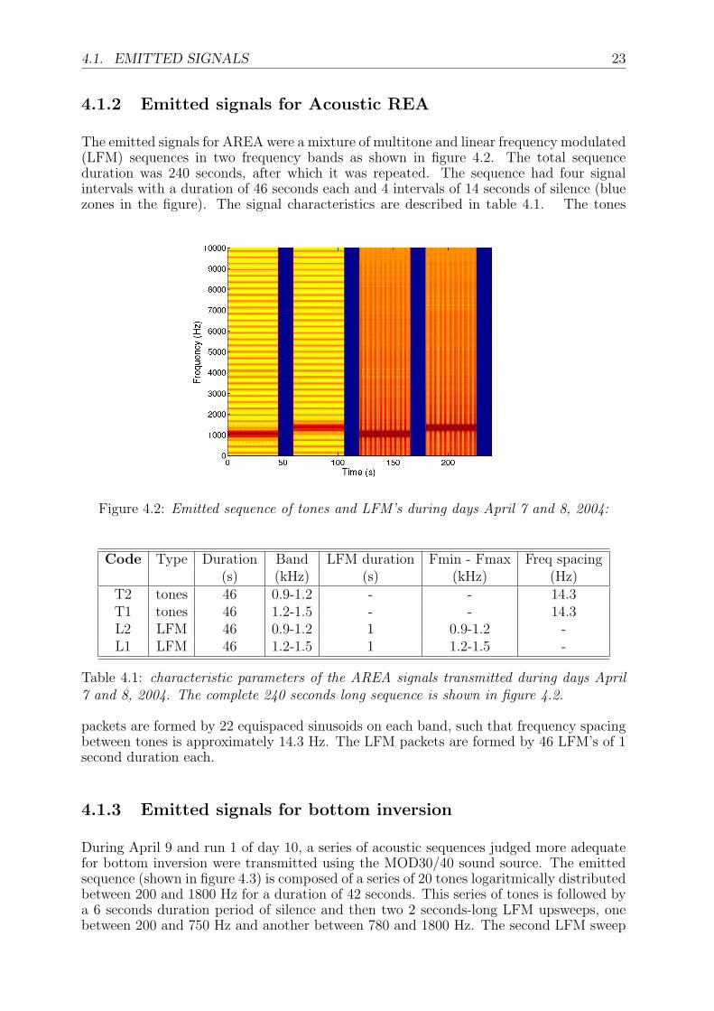
4.2 Emitted sequence of tones and LFM’s during days April 7 and 8, 2004: . . 23

4.3 emitted sequence of tones and LFM’s during days April 9 and run 1 ofApril 10, 2004: tones and LFMs. . . . . . . . . . . . . . . . . . . . . . . . 24

VII

VIII LIST OF FIGURES

4.4 pulse shape used as probe signal: root-root raised cosine (a) and its spec-trum (b), raised cosine (c) and its spectrum (d); continuous line is for 200symbols per second while dashed line is for 400 symbols per second. . . . . . 25

4.5 transmitted data: probe signal for code X (a), 84 s code X sequence (b) andfour codes A, B, C and D total data packet (c). . . . . . . . . . . . . . . . 25

4.6 spectograms of the transmitted signals: four distinct codes A, B, C, D (fromtop to bottom), repeated four times each, with 1 second probe-signal and 20seconds of data, giving a total duration of 84 seconds. The 336 second longstream of data is then continuously repeated with a silence of 24 seconds be-tween each repetition. The signals are transmitted with a carrier frequencyof 3600 Hz. . . . . . . . . . . . . . . . . . . . . . . . . . . . . . . . . . . . 26

4.7 Received signals on hydrophone 4 at 60 m depth, multitones and LFM’s:in frequency bands between 900 and 1500 Hz on day April 8, 2004 at 13:44UTC (a) and in frequency band 200 - 1800 Hz on day April 9, 2004 at12:53 UTC (b). . . . . . . . . . . . . . . . . . . . . . . . . . . . . . . . . . 27

4.8 AOB received signals during day April 9, 2004 as seen on the monitoringscreen aboard R/V Alliance. . . . . . . . . . . . . . . . . . . . . . . . . . . 27

4.9 AOB received underwater communication signals during day April 10, 2004on hydrophone 6 at 9:28:05 : in the upper subplot the 24 second silence thatmark the beginning of a new transmitted signal and then four times code A,four times code B, four times code C and four times code D with one secondof separation between them where the appropriate probe signal is transmitted. 28

4.10 time compression of the LFM signals in the 1.2 - 1.5 kHz band received onhydrophone 4 at nominal depth of 60 m during day April 7, 2004. . . . . . 28

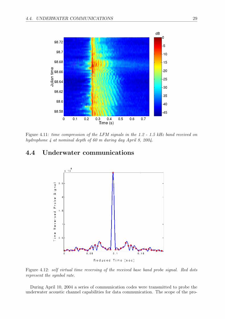
4.11 time compression of the LFM signals in the 1.2 - 1.5 kHz band received onhydrophone 4 at nominal depth of 60 m during day April 8, 2004. . . . . . 29

4.12 self virtual time reversing of the received base band probe signal. Red dotsrepresent the symbol rate. . . . . . . . . . . . . . . . . . . . . . . . . . . . . 29

4.13 pulse compression of the 1 s duration-800 Hz bandwidth probe signals alongthe PSK transmissions of run 2 on day April 10, 2004, received on hy-drophone 4 at nominal depth of 60 m. . . . . . . . . . . . . . . . . . . . . . 30

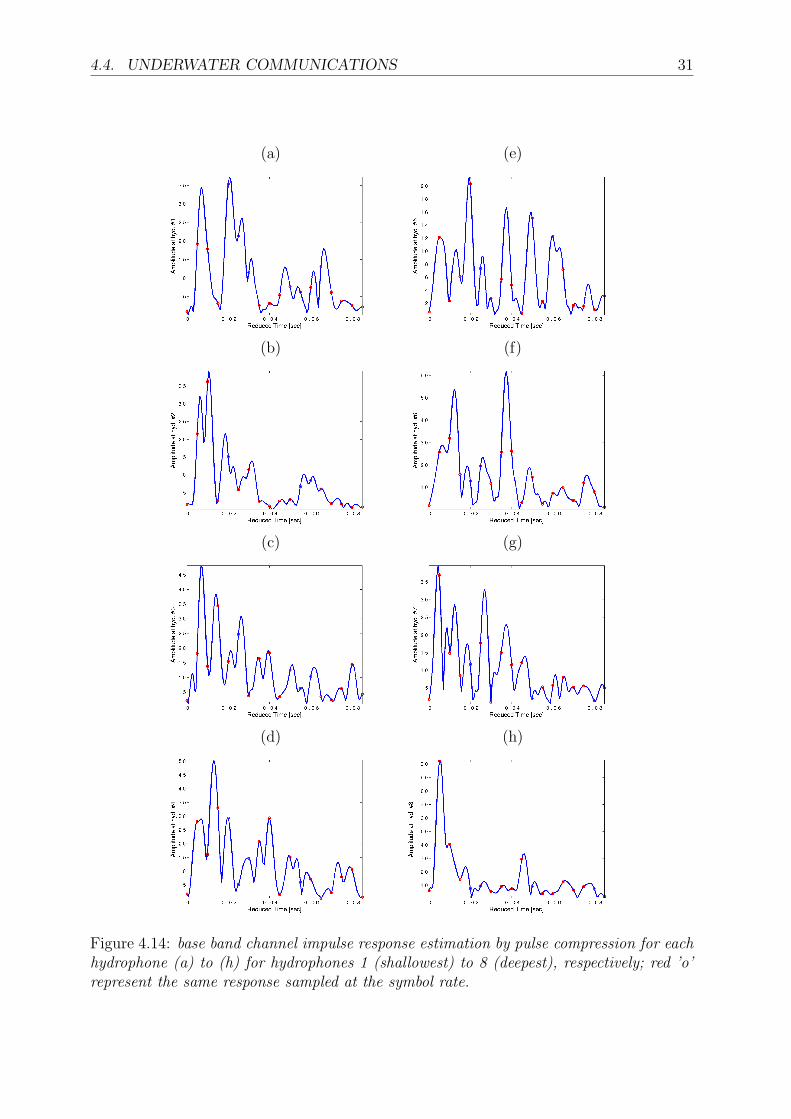
4.14 base band channel impulse response estimation by pulse compression foreach hydrophone (a) to (h) for hydrophones 1 (shallowest) to 8 (deepest),respectively; red ’o’ represent the same response sampled at the symbol rate. 31

Abstract

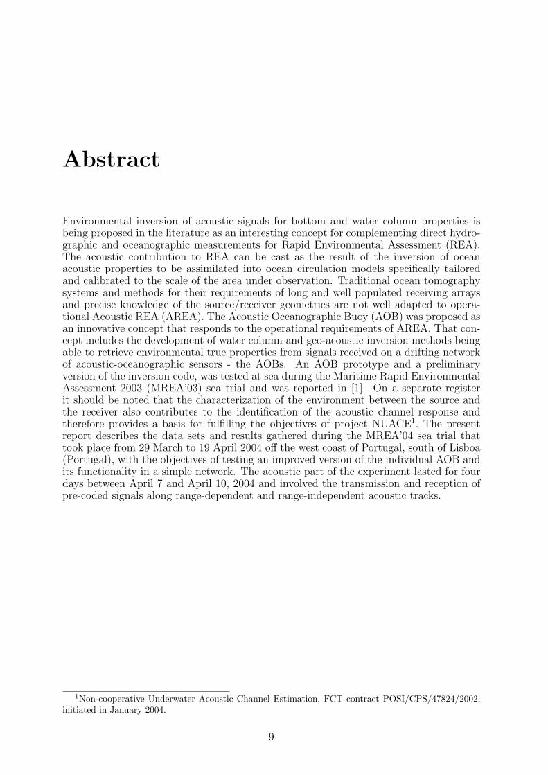
Environmental inversion of acoustic signals for bottom and water column properties isbeing proposed in the literature as an interesting concept for complementing direct hydro-graphic and oceanographic measurements for Rapid Environmental Assessment (REA).The acoustic contribution to REA can be cast as the result of the inversion of oceanacoustic properties to be assimilated into ocean circulation models specifically tailoredand calibrated to the scale of the area under observation. Traditional ocean tomographysystems and methods for their requirements of long and well populated receiving arraysand precise knowledge of the source/receiver geometries are not well adapted to opera-tional Acoustic REA (AREA). The Acoustic Oceanographic Buoy (AOB) was proposed asan innovative concept that responds to the operational requirements of AREA. That con-cept includes the development of water column and geo-acoustic inversion methods beingable to retrieve environmental true properties from signals received on a drifting networkof acoustic-oceanographic sensors - the AOBs. An AOB prototype and a preliminaryversion of the inversion code, was tested at sea during the Maritime Rapid EnvironmentalAssessment 2003 (MREA’03) sea trial and was reported in [1]. On a separate registerit should be noted that the characterization of the environment between the source andthe receiver also contributes to the identification of the acoustic channel response andtherefore provides a basis for fulfilling the objectives of project NUACE1. The presentreport describes the data sets and results gathered during the MREA’04 sea trial thattook place from 29 March to 19 April 2004 off the west coast of Portugal, south of Lisboa(Portugal), with the objectives of testing an improved version of the individual AOB andits functionality in a simple network. The acoustic part of the experiment lasted for fourdays between April 7 and April 10, 2004 and involved the transmission and reception ofpre-coded signals along range-dependent and range-independent acoustic tracks.

1Non-cooperative Underwater Acoustic Channel Estimation, FCT contract POSI/CPS/47824/2002,initiated in January 2004.

9

10 LIST OF FIGURES

intentionally blank

Chapter 1

Introduction

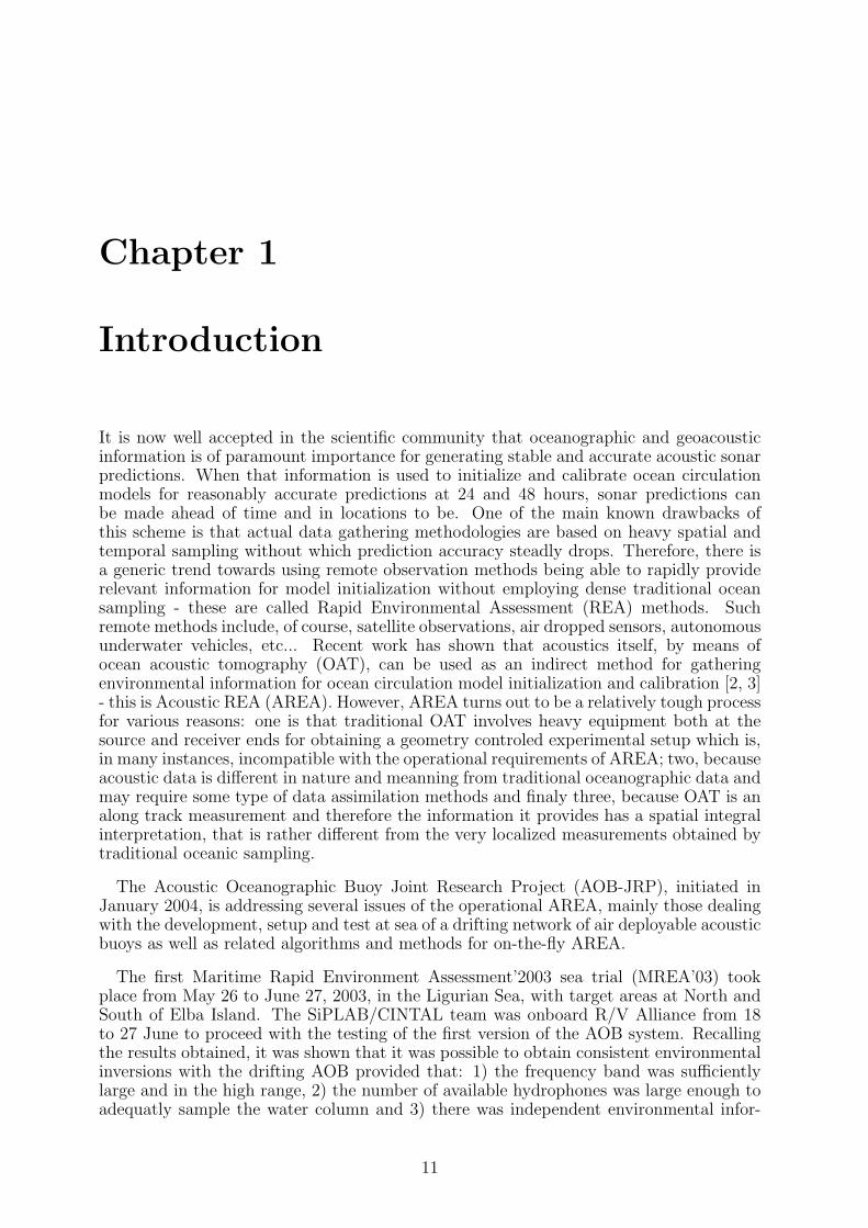
It is now well accepted in the scientific community that oceanographic and geoacousticinformation is of paramount importance for generating stable and accurate acoustic sonarpredictions. When that information is used to initialize and calibrate ocean circulationmodels for reasonably accurate predictions at 24 and 48 hours, sonar predictions canbe made ahead of time and in locations to be. One of the main known drawbacks ofthis scheme is that actual data gathering methodologies are based on heavy spatial andtemporal sampling without which prediction accuracy steadly drops. Therefore, there isa generic trend towards using remote observation methods being able to rapidly providerelevant information for model initialization without employing dense traditional oceansampling - these are called Rapid Environmental Assessment (REA) methods. Suchremote methods include, of course, satellite observations, air dropped sensors, autonomousunderwater vehicles, etc... Recent work has shown that acoustics itself, by means ofocean acoustic tomography (OAT), can be used as an indirect method for gatheringenvironmental information for ocean circulation model initialization and calibration [2, 3]- this is Acoustic REA (AREA). However, AREA turns out to be a relatively tough processfor various reasons: one is that traditional OAT involves heavy equipment both at thesource and receiver ends for obtaining a geometry controled experimental setup which is,in many instances, incompatible with the operational requirements of AREA; two, becauseacoustic data is different in nature and meanning from traditional oceanographic data andmay require some type of data assimilation methods and finaly three, because OAT is analong track measurement and therefore the information it provides has a spatial integralinterpretation, that is rather different from the very localized measurements obtained bytraditional oceanic sampling.

The Acoustic Oceanographic Buoy Joint Research Project (AOB-JRP), initiated inJanuary 2004, is addressing several issues of the operational AREA, mainly those dealingwith the development, setup and test at sea of a drifting network of air deployable acousticbuoys as well as related algorithms and methods for on-the-fly AREA.

The first Maritime Rapid Environment Assessment’2003 sea trial (MREA’03) tookplace from May 26 to June 27, 2003, in the Ligurian Sea, with target areas at North andSouth of Elba Island. The SiPLAB/CINTAL team was onboard R/V Alliance from 18to 27 June to proceed with the testing of the first version of the AOB system. Recallingthe results obtained, it was shown that it was possible to obtain consistent environmentalinversions with the drifting AOB provided that: 1) the frequency band was sufficientlylarge and in the high range, 2) the number of available hydrophones was large enough toadequatly sample the water column and 3) there was independent environmental infor-

11

12 CHAPTER 1. INTRODUCTION

mation to initialize the system (EOF computation) (see internal report [1] and conferenceproceedings [4]).

During the MREA’04 sea trial a second AOB test was performed. The AOB wasupgraded to 8 hydrophones and a 16 sensor thermistor chain was added. Another objectiveof the testing was to provide insight into the system setup and integration in a networkenvironment. The transmitted signals included frequency wide multitones and broadbandlinea frequency modulated (LFM) sweeps for environmental inversion and PSK sequencesfor underwater communication purposes (NUACE).

This report is organized as follows: chapter 2 gives an overall description of the hardwareand software changes introduced in the AOB relative to the version used in 2003; chapter3 describes the MREA’04 sea trial workframe, ground truth measurements and deploy-ment geometries; chapter 4 shows the acoustic data received on the AOB and the resultsobtained; finally, conclusions and future developments are drawn in chapter 5. Oceancirculation modeling and data assimilation are to be dealt with in a separate report. Anadditional DVD contains the various data sets and useful data handling routines.

Chapter 2

The Acoustic Oceanographic Buoy

2.1 AOB hardware

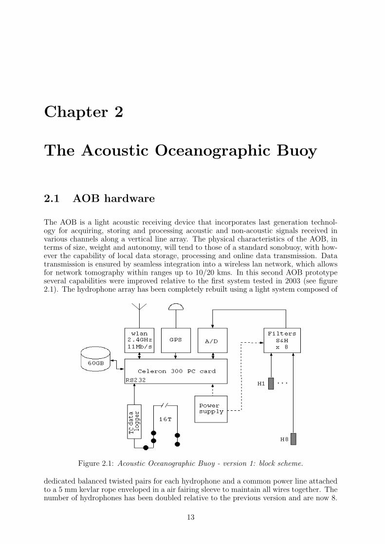
The AOB is a light acoustic receiving device that incorporates last generation technol-ogy for acquiring, storing and processing acoustic and non-acoustic signals received invarious channels along a vertical line array. The physical characteristics of the AOB, interms of size, weight and autonomy, will tend to those of a standard sonobuoy, with how-ever the capability of local data storage, processing and online data transmission. Datatransmission is ensured by seamless integration into a wireless lan network, which allowsfor network tomography within ranges up to 10/20 kms. In this second AOB prototypeseveral capabilities were improved relative to the first system tested in 2003 (see figure2.1). The hydrophone array has been completely rebuilt using a light system composed of

Figure 2.1: Acoustic Oceanographic Buoy - version 1: block scheme.

dedicated balanced twisted pairs for each hydrophone and a common power line attachedto a 5 mm kevlar rope enveloped in a air fairing sleeve to maintain all wires together. Thenumber of hydrophones has been doubled relative to the previous version and are now 8.

13

14 CHAPTER 2. THE ACOUSTIC OCEANOGRAPHIC BUOY

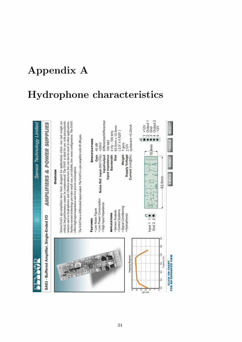
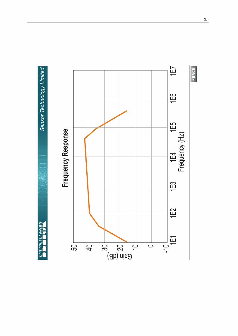
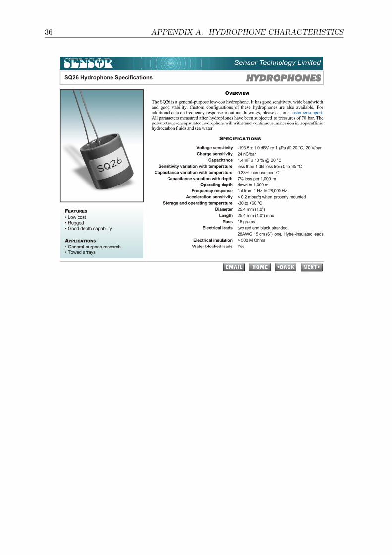
Hydrophone depths are as follows: 10, 15, 55, 60, 65, 70, 75 and 80 m. The hydrophoneswere manufactured by Sensor Technology (Canada) and their frequency response andoverall characteristics are shown in appendix A.

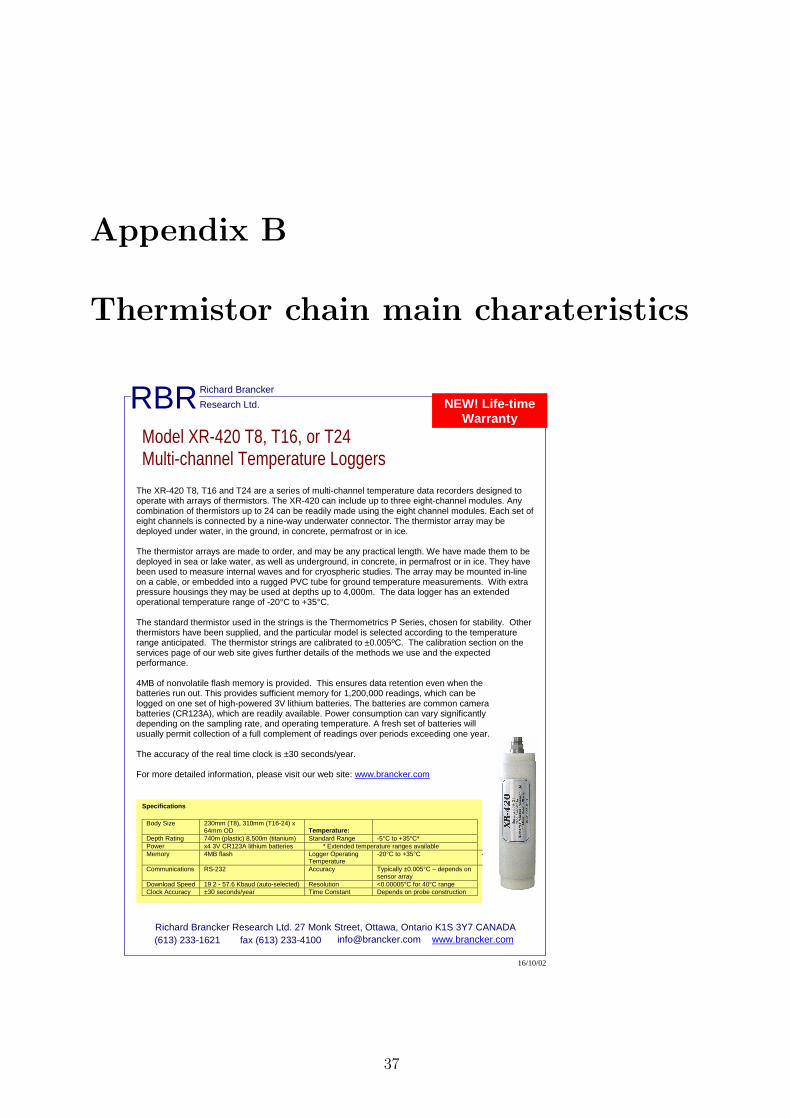
The other subsystem that was added in the actual version of the AOB is the thermistorchain (TC) for online water column temperature monitoring. This subsystem was pur-chased from RBR Ltd. (Canada) and is mainly composed of a data logger that monitorsthe 16-sensor-80 m long equispaced TC array. The main characteristics of the TC areshown in appendix B. The TC data logger is interrogated by the AOB’s CPU at regularintervals so that synoptic water column temperature measurements are provided to theremote user together with concurrent acoustic data. All the other features of the AOB,such as the Wlan capabilities, on the water ON/OFF circuitry and on board easy batterycharge and data transfer were maintained (see report [1] for details).

2.2 AOB software

(a) (b)

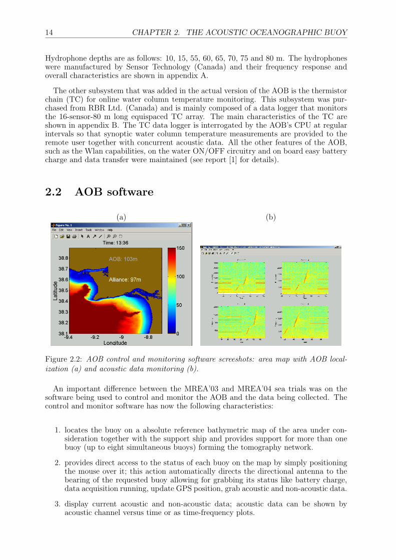
Figure 2.2: AOB control and monitoring software screeshots: area map with AOB local-ization (a) and acoustic data monitoring (b).

An important difference between the MREA’03 and MREA’04 sea trials was on thesoftware being used to control and monitor the AOB and the data being collected. Thecontrol and monitor software has now the following characteristics:

1. locates the buoy on a absolute reference bathymetric map of the area under con-sideration together with the support ship and provides support for more than onebuoy (up to eight simultaneous buoys) forming the tomography network.

2. provides direct access to the status of each buoy on the map by simply positioningthe mouse over it; this action automatically directs the directional antenna to thebearing of the requested buoy allowing for grabbing its status like battery charge,data acquisition running, update GPS position, grab acoustic and non-acoustic data.

3. display current acoustic and non-acoustic data; acoustic data can be shown byacoustic channel versus time or as time-frequency plots.

2.2. AOB SOFTWARE 15

Examples of the various displays provided by this application are shown in figures2.2(a) and (b). The data inversion procedure used during the MREA’03 sea trial, wasbased on code previously developed for Blind Ocean Acoustic Tomography (BOAT) [5, 6]with, however, completely different settings for the parameter search bounds and geneticalgorithms (GA) conversion parameters, taking into account that source position and localbathymetry was approximately known. It should be remarked that BOAT aims at theinversion of ocean properties and therefore at the identification of the acoustic channellinking the source and receiver, full filing therefore also the aims of project NUACE. Asa complement of information and in order to explore a larger frequency band than thatnormally used in AREA, phase shift keying (PSK) data sequences were also trasmittedand received during the MREA’04 sea trial. This data set are also described here but thedetailed processing results are left for a separate report. Unlike in the MREA’03, duringthe MREA’04 sea trial specific data codes were transmitted and received on the AOB forwater column and bottom geo-acoustic inversion, which details and final results are alsoleft for a separate publication.

Chapter 3

The MREA’04 sea trial

3.1 Generalities and sea trial area

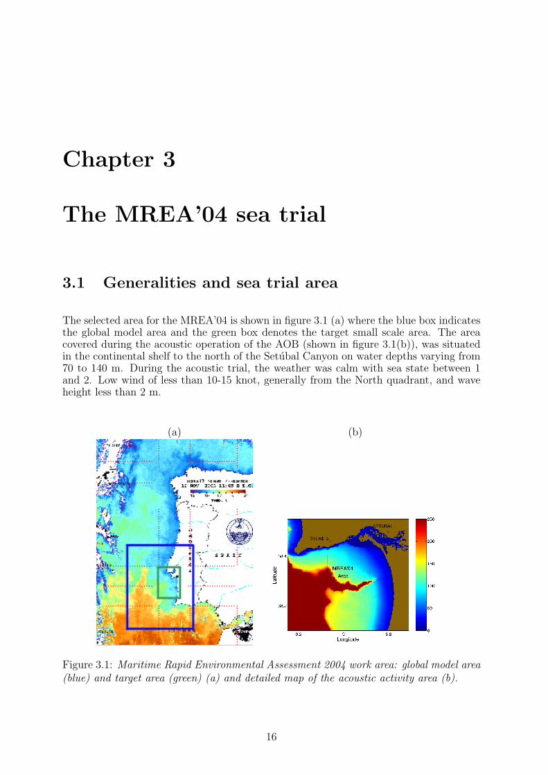
The selected area for the MREA’04 is shown in figure 3.1 (a) where the blue box indicatesthe global model area and the green box denotes the target small scale area. The areacovered during the acoustic operation of the AOB (shown in figure 3.1(b)), was situatedin the continental shelf to the north of the Setubal Canyon on water depths varying from70 to 140 m. During the acoustic trial, the weather was calm with sea state between 1and 2. Low wind of less than 10-15 knot, generally from the North quadrant, and waveheight less than 2 m.

(a) (b)

Figure 3.1: Maritime Rapid Environmental Assessment 2004 work area: global model area(blue) and target area (green) (a) and detailed map of the acoustic activity area (b).

16

3.2. GROUND TRUTH MEASUREMENTS 17

3.2 Ground truth measurements

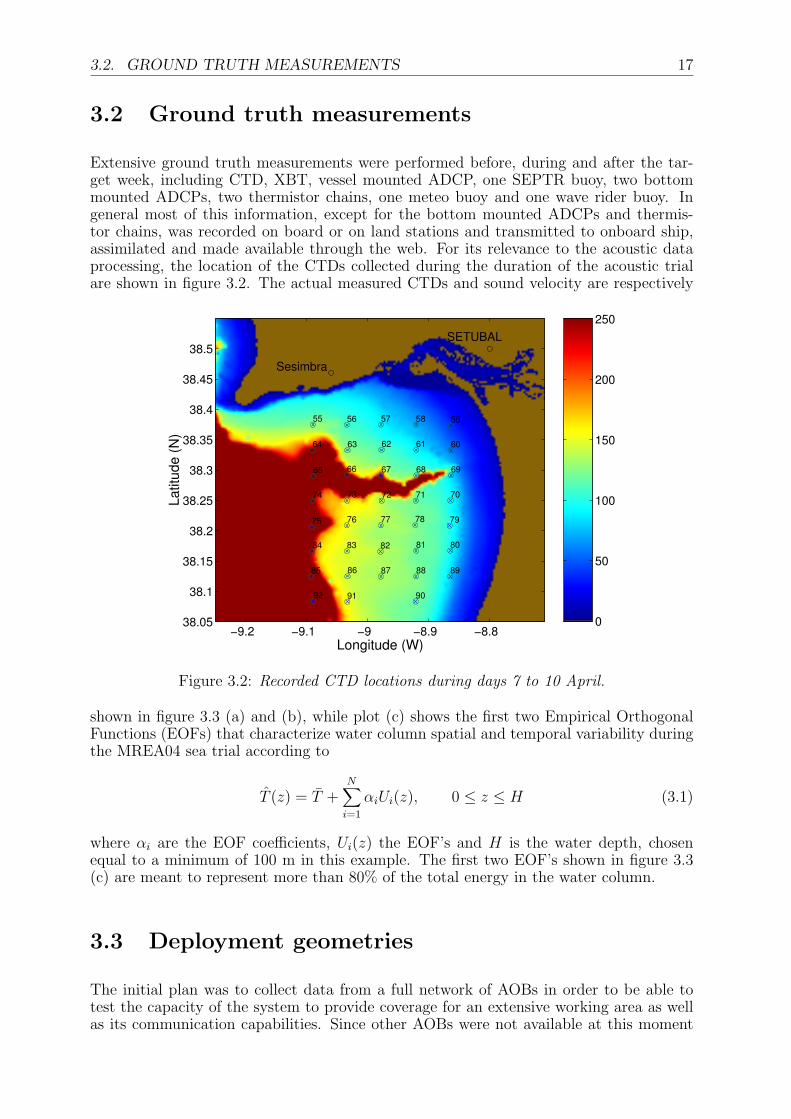
Extensive ground truth measurements were performed before, during and after the tar-get week, including CTD, XBT, vessel mounted ADCP, one SEPTR buoy, two bottommounted ADCPs, two thermistor chains, one meteo buoy and one wave rider buoy. Ingeneral most of this information, except for the bottom mounted ADCPs and thermis-tor chains, was recorded on board or on land stations and transmitted to onboard ship,assimilated and made available through the web. For its relevance to the acoustic dataprocessing, the location of the CTDs collected during the duration of the acoustic trialare shown in figure 3.2. The actual measured CTDs and sound velocity are respectively

Longitude (W)

Latit

ude

(N)

Sesimbra

SETUBAL

55 56 57 58 59

6061626364

65 66 67 68 69

7071727374

75 76 77 78 79

8081828384

85 86 87 88 89

909192

−9.2 −9.1 −9 −8.9 −8.838.05

38.1

38.15

38.2

38.25

38.3

38.35

38.4

38.45

38.5

0

50

100

150

200

250

Figure 3.2: Recorded CTD locations during days 7 to 10 April.

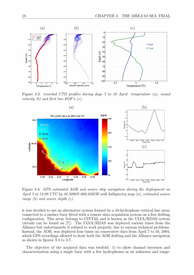
shown in figure 3.3 (a) and (b), while plot (c) shows the first two Empirical OrthogonalFunctions (EOFs) that characterize water column spatial and temporal variability duringthe MREA04 sea trial according to

T (z) = T +N∑

i=1

αiUi(z), 0 ≤ z ≤ H (3.1)

where αi are the EOF coefficients, Ui(z) the EOF’s and H is the water depth, chosenequal to a minimum of 100 m in this example. The first two EOF’s shown in figure 3.3(c) are meant to represent more than 80% of the total energy in the water column.

3.3 Deployment geometries

The initial plan was to collect data from a full network of AOBs in order to be able totest the capacity of the system to provide coverage for an extensive working area as wellas its communication capabilities. Since other AOBs were not available at this moment

18 CHAPTER 3. THE MREA’04 SEA TRIAL

(a) (b) (c)

1500 1505 1510 1515−900

−800

−700

−600

−500

−400

−300

−200

−100

0

Sound velocity (m/s)11 12 13 14 15 16

−900

−800

−700

−600

−500

−400

−300

−200

−100

0

Temperature °C

Dep

th (m

)

meanctds

−0.2 0 0.2

0

10

20

30

40

50

60

70

80

90

100

1st EOF

2nd EOF

Temperature (oC)

Dep

th (m

)

Figure 3.3: recorded CTD profiles during days 7 to 10 April: temperature (a), soundvelocity (b) and first two EOF’s (c).

(a) (b)

97.58 97.6 97.62 97.64 97.66 97.68 97.70

0.5

1

1.5

2

2.5

3

3.5

4

4.5

Julian time

Ran

ge (k

m)

(c)

97.58 97.6 97.62 97.64 97.66 97.68 97.7

0

20

40

60

80

100

120

Julian time

Dep

th (m

)

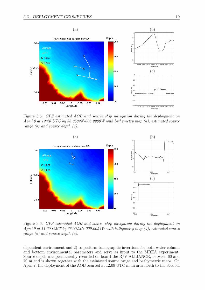
Figure 3.4: GPS estimated AOB and source ship navigation during the deployment onApril 7 at 12:09 UTC by 38.3096N-009.0205W with bathymetry map (a), estimated sourcerange (b) and source depth (c).

it was decided to use an alternative system formed by a 16-hydrophone vertical line arrayconnected to a surface buoy fitted with a remote data acquisition system on a free driftingconfiguration. This array belongs to CINTAL and is known as the ULVA/RDAS system(details can be found on [7]). The ULVA/RDAS was deployed various times from theAlliance but unfortunately it refused to work properly, due to various technical problems.Instead, the AOB, was deployed four times on consecutive days from April 7 to 10, 2004,which GPS recordings allowed to draw both the AOB drifting and the Alliance navigationas shown in figures 3.4 to 3.7.

The objective of the acquired data was twofold: 1) to allow channel inversion andcharacterization using a single buoy with a few hydrophones in an unknown and range-

3.3. DEPLOYMENT GEOMETRIES 19

(a) (b)

98.58 98.6 98.62 98.64 98.66 98.68 98.7 98.720

0.5

1

1.5

2

2.5

3

3.5

4

Julian time

Ran

ge (k

m)

(c)

98.58 98.6 98.62 98.64 98.66 98.68 98.7 98.72

0

20

40

60

80

100

120

Julian time

Dep

th (m

)

Figure 3.5: GPS estimated AOB and source ship navigation during the deployment onApril 8 at 12:26 UTC by 38.3532N-008.9989W with bathymetry map (a), estimated sourcerange (b) and source depth (c).

(a) (b)

99.5 99.6 99.70

0.5

1

1.5

2

2.5

3

3.5

Julian time

Ran

ge (k

m)

(c)

99.5 99.6 99.7

0

20

40

60

80

100

120

Julian time

Dep

th (m

)

Figure 3.6: GPS estimated AOB and source ship navigation during the deployment onApril 9 at 11:35 GMT by 38.3743N-009.0047W with bathymetry map (a), estimated sourcerange (b) and source depth (c).

dependent environment and 2) to perform tomographic inversions for both water columnand bottom environmental parameters and serve as input to the MREA experiment.Source depth was permanently recorded on board the R/V ALLIANCE, between 60 and70 m and is shown together with the estimated source range and bathymetric maps. OnApril 7, the deployment of the AOB ocurred at 12:09 UTC in an area north to the Setubal

20 CHAPTER 3. THE MREA’04 SEA TRIAL

Canyon close to the border of the continental platform with an approximate water depthof 120-130 m. During the deployment the AOB slowly drifted approximately 1 km to theEast (see figure 3.4). Source - receiver range varied from 1 up to 5 km on a variable

(a) (b)

100.36 100.37 100.38 100.39 100.40

0.2

0.4

0.6

0.8

1

1.2

1.4

1.6

1.8

Julian time

Ran

ge (k

m)

(c)

100.36 100.37 100.38 100.39 100.4

0

20

40

60

80

100

120

Julian time

Dep

th (m

)

Figure 3.7: GPS estimated AOB and source ship navigation during the deployment onApril 10 (run 1) at 07:55 UTC by 38.3737N-009.0053W with bathymetry map (a), esti-mated source range (b) and source depth (c).

(a) (b)

100.46100.47100.48100.49100.5100.51100.52100.53100.540

1

2

3

4

5

6

Julian time

Ran

ge (k

m)

(c)

100.46100.47100.48100.49100.5100.51100.52100.53100.54

0

20

40

60

80

100

120

Julian time

Dep

th (m

)

Figure 3.8: GPS estimated AOB and source ship navigation during the deployment onApril 10 (run 2) started at 10:49 UTC with bathymetry map (a), estimated source range(b) and source depth (c).

water depth area close or over the continental platform border. The second deployment

3.3. DEPLOYMENT GEOMETRIES 21

took place on April 8 at 12:26 UTC in a flat area with depths varying between 100 and110 m. During the 3.5 hours acoustic run the AOB drifted approximately 3 kms to theEast, while the NRV ALLIANCE accomplished a complex pattern to the South, Eastand North relative to the free drifting track of the AOB as shown in figure 3.5. On dayApril 9, 2004, the AOB was deployed at 11:35 UTC to the South of the source ship at anapproximate range of 2.5 km. Along the recording interval the ship was closing range tothe AOB down to slightly less than 1 km and then rapidly moved North to approximately3.5 km from the AOB (figure 3.6). The last day for acoustic data was April 10, 2004,where the AOB was deployed at 7:55 UTC. The acoustic run 1 started at a close rangeof 0.6 km to the South of the AOB and the source progressively opened range to theSouth - East along an approximately range independant path up to 2 km (figure 3.7).The broadband source was recovered and the NRV Alliance moved to approximately 6km range from the AOB along a nearly bathymetric range independant path of 110 mwater depth were she made a station (figure 3.8). During this second run of day April 10,the MOD30/40 was lowered at depths of 10 and 70 m, transmitting acoustic signals forbottom inversion.

Chapter 4

Acoustic data

4.1 Emitted signals

4.1.1 Acoustic sources

Acoustic signals were emitted from R/V Alliance mainly using two types of transducers:a broadband sound source covering the band 180 to 5000 Hz for water column inversionand a low frequency MOD30/40 transducer for bottom inversion. The broadband soundsource was used on April 7, 8 and run 2 of April 10, while the MOD30/40 transducerwas used on April 9 and run 1 of April 10. The broadband sound source was actuallycomposed of two transducers, for the low and high frequency bands, mounted on a singletwo body. The low frequency transducer was a HX90G (SN51) covering the band 180-600Hz, while the high-frequency tansducer was an ITC2010 (SN508) roughly covering theband 700-5000 Hz. The transducers were driven by a Instruments Inc. power amplifier.Source level curves of the broadband sound source are shown in figure 4.1(a) while theMOD30/40 frequency response is shown in 4.1(b).

(a) (b)

102 103100

105

110

115

120

125

130

135

140

Frequency (Hz)

Sou

rce

leve

l (db

)

Figure 4.1: transmitting source frequency response: broadband source (a) and MOD30/40- SN2 (Seneca Lake, Dec 1990) (b).

22

4.1. EMITTED SIGNALS 23

4.1.2 Emitted signals for Acoustic REA

The emitted signals for AREA were a mixture of multitone and linear frequency modulated(LFM) sequences in two frequency bands as shown in figure 4.2. The total sequenceduration was 240 seconds, after which it was repeated. The sequence had four signalintervals with a duration of 46 seconds each and 4 intervals of 14 seconds of silence (bluezones in the figure). The signal characteristics are described in table 4.1. The tones

Figure 4.2: Emitted sequence of tones and LFM’s during days April 7 and 8, 2004:

Code Type Duration Band LFM duration Fmin - Fmax Freq spacing(s) (kHz) (s) (kHz) (Hz)

T2 tones 46 0.9-1.2 - - 14.3T1 tones 46 1.2-1.5 - - 14.3L2 LFM 46 0.9-1.2 1 0.9-1.2 -L1 LFM 46 1.2-1.5 1 1.2-1.5 -

Table 4.1: characteristic parameters of the AREA signals transmitted during days April7 and 8, 2004. The complete 240 seconds long sequence is shown in figure 4.2.

packets are formed by 22 equispaced sinusoids on each band, such that frequency spacingbetween tones is approximately 14.3 Hz. The LFM packets are formed by 46 LFM’s of 1second duration each.

4.1.3 Emitted signals for bottom inversion

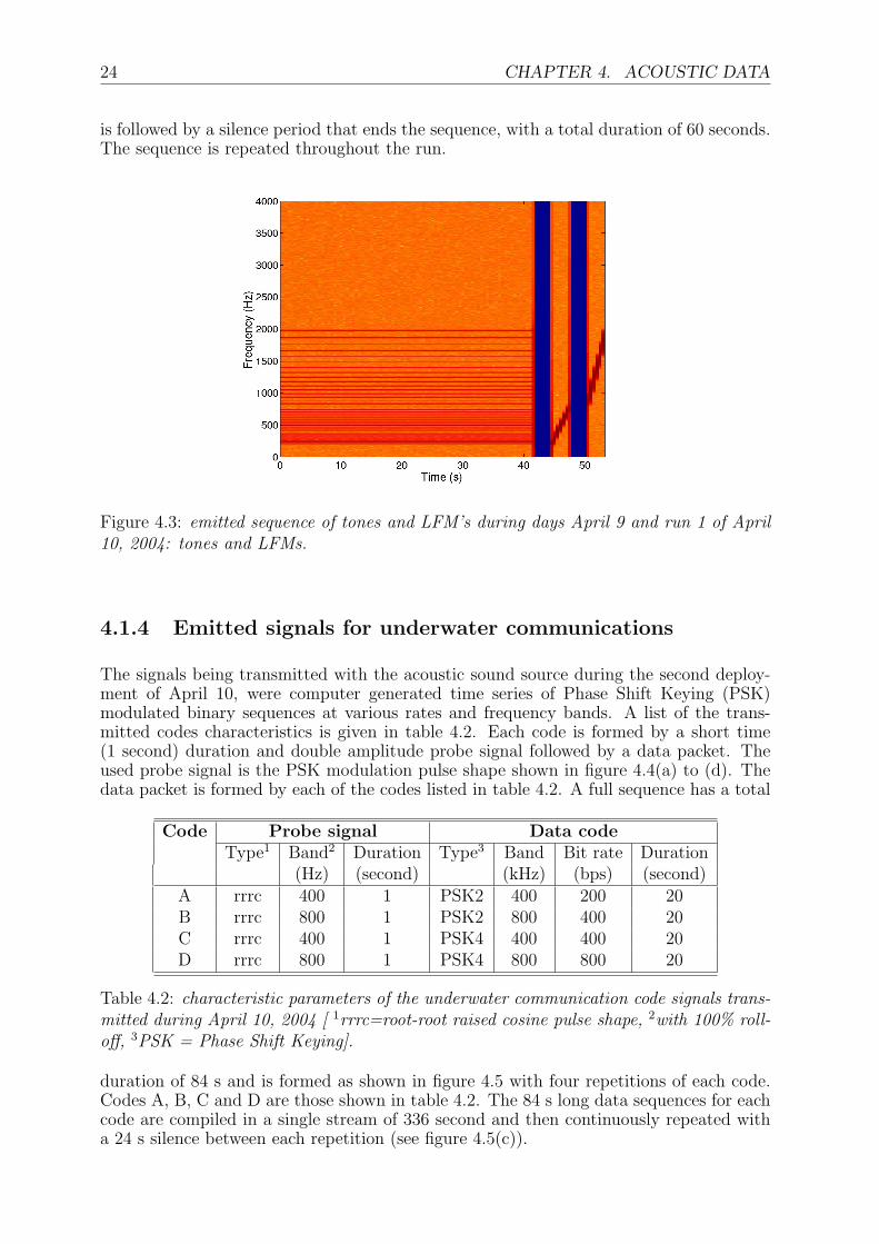
During April 9 and run 1 of day 10, a series of acoustic sequences judged more adequatefor bottom inversion were transmitted using the MOD30/40 sound source. The emittedsequence (shown in figure 4.3) is composed of a series of 20 tones logaritmically distributedbetween 200 and 1800 Hz for a duration of 42 seconds. This series of tones is followed bya 6 seconds duration period of silence and then two 2 seconds-long LFM upsweeps, onebetween 200 and 750 Hz and another between 780 and 1800 Hz. The second LFM sweep

24 CHAPTER 4. ACOUSTIC DATA

is followed by a silence period that ends the sequence, with a total duration of 60 seconds.The sequence is repeated throughout the run.

Figure 4.3: emitted sequence of tones and LFM’s during days April 9 and run 1 of April10, 2004: tones and LFMs.

4.1.4 Emitted signals for underwater communications

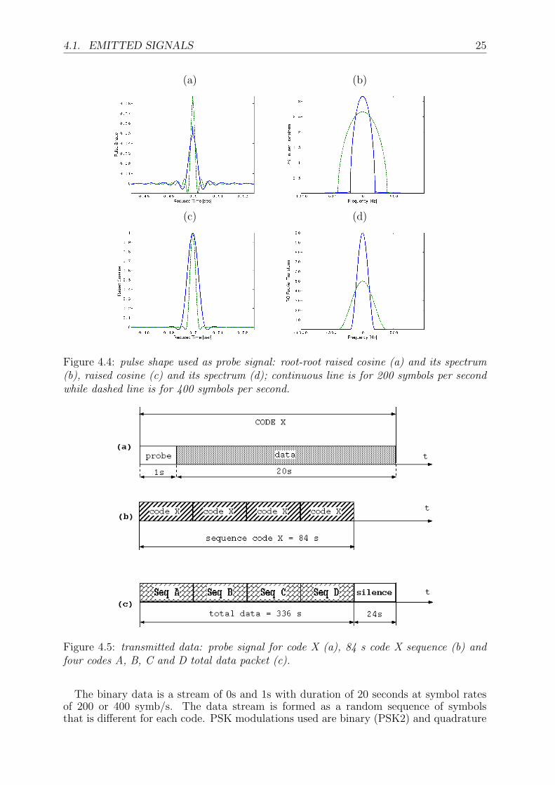
The signals being transmitted with the acoustic sound source during the second deploy-ment of April 10, were computer generated time series of Phase Shift Keying (PSK)modulated binary sequences at various rates and frequency bands. A list of the trans-mitted codes characteristics is given in table 4.2. Each code is formed by a short time(1 second) duration and double amplitude probe signal followed by a data packet. Theused probe signal is the PSK modulation pulse shape shown in figure 4.4(a) to (d). Thedata packet is formed by each of the codes listed in table 4.2. A full sequence has a total

Code Probe signal Data codeType1 Band2 Duration Type3 Band Bit rate Duration

(Hz) (second) (kHz) (bps) (second)A rrrc 400 1 PSK2 400 200 20B rrrc 800 1 PSK2 800 400 20C rrrc 400 1 PSK4 400 400 20D rrrc 800 1 PSK4 800 800 20

Table 4.2: characteristic parameters of the underwater communication code signals trans-mitted during April 10, 2004 [ 1rrrc=root-root raised cosine pulse shape, 2with 100% roll-off, 3PSK = Phase Shift Keying].

duration of 84 s and is formed as shown in figure 4.5 with four repetitions of each code.Codes A, B, C and D are those shown in table 4.2. The 84 s long data sequences for eachcode are compiled in a single stream of 336 second and then continuously repeated witha 24 s silence between each repetition (see figure 4.5(c)).

4.1. EMITTED SIGNALS 25

(a) (b)

(c) (d)

Figure 4.4: pulse shape used as probe signal: root-root raised cosine (a) and its spectrum(b), raised cosine (c) and its spectrum (d); continuous line is for 200 symbols per secondwhile dashed line is for 400 symbols per second.

Figure 4.5: transmitted data: probe signal for code X (a), 84 s code X sequence (b) andfour codes A, B, C and D total data packet (c).

The binary data is a stream of 0s and 1s with duration of 20 seconds at symbol ratesof 200 or 400 symb/s. The data stream is formed as a random sequence of symbolsthat is different for each code. PSK modulations used are binary (PSK2) and quadrature


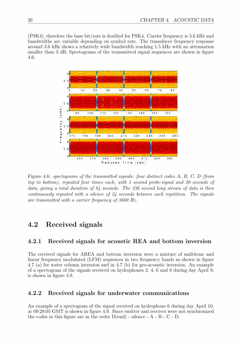
(PSK4), therefore the base bit/rate is doubled for PSK4. Carrier frequency is 3.6 kHz andbandwidths are variable depending on symbol rate. The transducer frequency responsearound 3.6 kHz shows a relatively wide bandwidth reaching 1.5 kHz with an attenuationsmaller than 3 dB. Spectograms of the transmitted signal sequences are shown in figure4.6.

Figure 4.6: spectograms of the transmitted signals: four distinct codes A, B, C, D (fromtop to bottom), repeated four times each, with 1 second probe-signal and 20 seconds ofdata, giving a total duration of 84 seconds. The 336 second long stream of data is thencontinuously repeated with a silence of 24 seconds between each repetition. The signalsare transmitted with a carrier frequency of 3600 Hz.

4.2 Received signals

4.2.1 Received signals for acoustic REA and bottom inversion

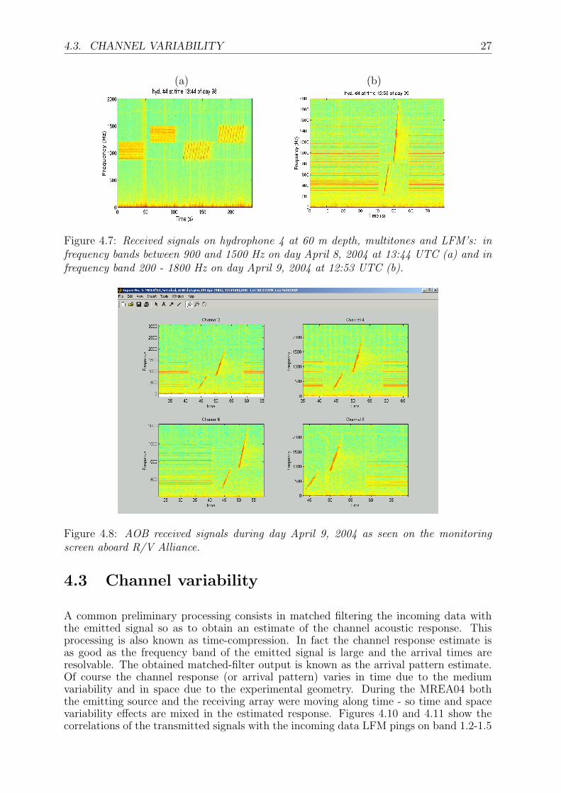
The received signals for AREA and bottom inversion were a mixture of multitone andlinear frequency modulated (LFM) sequences in two frequency bands as shown in figure4.7 (a) for water column inversion and in 4.7 (b) for geo-acoustic inversion. An exampleof a spectogram of the signals received on hydrophones 2, 4, 6 and 8 during day April 9,is shown in figure 4.8.

4.2.2 Received signals for underwater communications

An example of a spectogram of the signal received on hydrophone 6 during day April 10,at 09:28:05 GMT is shown in figure 4.9. Since emitter and receiver were not synchronizedthe codes in this figure are in the order D(end) - silence - A - B - C - D.

4.3. CHANNEL VARIABILITY 27

(a) (b)

Figure 4.7: Received signals on hydrophone 4 at 60 m depth, multitones and LFM’s: infrequency bands between 900 and 1500 Hz on day April 8, 2004 at 13:44 UTC (a) and infrequency band 200 - 1800 Hz on day April 9, 2004 at 12:53 UTC (b).

Figure 4.8: AOB received signals during day April 9, 2004 as seen on the monitoringscreen aboard R/V Alliance.

4.3 Channel variability

A common preliminary processing consists in matched filtering the incoming data withthe emitted signal so as to obtain an estimate of the channel acoustic response. Thisprocessing is also known as time-compression. In fact the channel response estimate isas good as the frequency band of the emitted signal is large and the arrival times areresolvable. The obtained matched-filter output is known as the arrival pattern estimate.Of course the channel response (or arrival pattern) varies in time due to the mediumvariability and in space due to the experimental geometry. During the MREA04 boththe emitting source and the receiving array were moving along time - so time and spacevariability effects are mixed in the estimated response. Figures 4.10 and 4.11 show thecorrelations of the transmitted signals with the incoming data LFM pings on band 1.2-1.5


Figure 4.9: AOB received underwater communication signals during day April 10, 2004on hydrophone 6 at 9:28:05 : in the upper subplot the 24 second silence that mark thebeginning of a new transmitted signal and then four times code A, four times code B, fourtimes code C and four times code D with one second of separation between them wherethe appropriate probe signal is transmitted.

Figure 4.10: time compression of the LFM signals in the 1.2 - 1.5 kHz band received onhydrophone 4 at nominal depth of 60 m during day April 7, 2004.

kHz, received on hydrophone 4 (60 m nominal depth) during the run of days April 7and 8, respectively. The multipath structure can be clearly correlated with the source -receiver variable range with increasing and decreasing number of visible arrivals from 2up to 7 arrival packets, generally accompained by a pre-peak faster than water arrivals atclose ranges.

4.4. UNDERWATER COMMUNICATIONS 29

Figure 4.11: time compression of the LFM signals in the 1.2 - 1.5 kHz band received onhydrophone 4 at nominal depth of 60 m during day April 8, 2004.

4.4 Underwater communications

Figure 4.12: self virtual time reversing of the received base band probe signal. Red dotsrepresent the symbol rate.

During April 10, 2004 a series of communication codes were transmitted to probe theunderwater acoustic channel capabilities for data communication. The scope of the pro-


cessing is to use the virtual time reversal concept as presented in [8, 9]. Very simplyspeaking, the idea is to use the received probe signal as an image of the signal pulse shapeconvolved with the channel impulse response to match-filter the received data sequencethat follows the probe signal. In doing this, there is the hope that the acoustic channelis sufficiently stable to hold during the data sequence duration, which is 20 seconds inour case. The ideal (no channel or geometric variability) virtual time reversal responseof the whole array mainly depends on the number of hydrophones and their localizationon the water column. Figure 4.12 shows an estimate of the ideal virtual time reversalresponse for the array configuration used during the MREA’04 data set of day April 10.The red dots represent the symbol rate, so one can see that the virtual time reversal im-pulse response main lobe is narrower than a symbol interval resulting therefore on a ISIless output data stream. In order to obtain an idea of the channel time variability that

Figure 4.13: pulse compression of the 1 s duration-800 Hz bandwidth probe signals alongthe PSK transmissions of run 2 on day April 10, 2004, received on hydrophone 4 atnominal depth of 60 m.

the virtual time reversal (or equivalently any channel equalizer) has to cope with, the 1 sduration probe signal before each data packet was pulse compressed with the transmittedreplica. The results obtained along the data set of run 2 of April 10, 2004, using the800 Hz probe of hydrophone 4 (60 m depth), are shown in figure 4.13. The multipathstructure can be clearly associated with the relative source -re ceiver movement alongtime by close observation of figure 3.8. However, one thing is to account for time variabil-ity and another is to cope with spatial variability, which is the main goal behind virtualretrofocusing for underwater communications. Figure 4.14(a) to (h) shows the moduleof the baseband channel impulse response estimate for hydrophones 1 (shallowest) to 8(deepest), respectively. A strong multipath can be noticed, that spans up to 22 symbolsand a strong variability between the channels that is evident in the top hydrophones 10and 15 meters depth and in the bottom hydrophones 55, 60, 65, 70, 75, 80 meters depth.It is remarkable to see how that strong spatial variability is perfectly accounted for toform the ideal response of previous figure 4.12.

4.4. UNDERWATER COMMUNICATIONS 31

(a) (e)

(b) (f)

(c) (g)

(d) (h)

Figure 4.14: base band channel impulse response estimation by pulse compression for eachhydrophone (a) to (h) for hydrophones 1 (shallowest) to 8 (deepest), respectively; red ’o’represent the same response sampled at the symbol rate.

Chapter 5

Conclusions and future developments

The Maritime Rapid Environmental Assessment 2004 (MREA’04) sea trial is the second ina series of experiments aiming at proving the concept of bringing together the expertise ofvarious fields for a rapid and consistent estimation of a shallow water area. Contributionsfrom ocean circulation modelling, remote sensing, direct CTD, wave height and sea currentmeasurements and acoustics are assimilated into a single web based framework for easydata exchange and manipulation, aiming at a final as accurate as possible 24 and 48hours forecast of environmental conditions in the area. This report mainly describes theacoustic testing data set gathered during the MREA’04 effort. The acoustic data set canbe divided in three subsets: 1) the water column REA subset, 2) the geoacoustic REAsubset and 3) the underwater communications subset.

This report describes the experimental setup for whole the acoustic part of the MREA’04and gives data processing details for subsets 1) and 3), while for subset 2) details are underthe responsability of J.-P. Hermand and Mathias Meyer from ULB (to be made availablein a separate report). Preliminary results show that the AOB is a reliable system for un-derwater acoustic data gathering, giving low-noise highly accurate recordings at all timesand in a wide frequency band.

32

Bibliography

[1] Jesus S., Silva A., and Soares C. Acoustic oceanographic buoy test during the mrea’03sea trial. Internal Report Rep. 04/03, SiPLAB/CINTAL, Universidade do Algarve,Faro, Portugal, November 2003.

[2] Elisseeff P., Schmidt H., and Xu W. Ocean acoustic tomography as a data assimilationproblem. IEEE Journal of Oceanic Engineering, 27(2):275–282, 2002.

[3] Lermusieux P.F.J. and Chiu C.-S. Four-dimensional data assimilation for coupledphysical-acoustical fields. In Pace and Jensen, editors, Impact of Littoral EnvironmentVariability on Acoustic Predictions and Sonar Performance, pages 417–424, Kluwer,September 2002.

[4] S.M. Jesus, C. Soares, A.J. Silva, and E. Coelho. Acoustic oceanographic buoy testingduring the maritime rapid environmental assessment 2003 sea trial. In Proc. EuropeanConference on Underwater Acoustic, Delft, The Netherlands, July 2004.

[5] S.M. Jesus, C. Soares, J. Onofre, and P. Picco. Blind ocean acoustic tomography:Experimental results on the intifante’00 data set. In Proc. Sixth of European Conf.on Underwater Acoust., ECUA’02, Gdansk, Poland, June 2002.

[6] S.M. Jesus, c. Soares, J. Onofre, E. Coelho, and P. Picco. Experimental testing ofthe blind ocean acoustic tomography concept. In Pace and Jensen, editors, Impactof Littoral Environment Variability on Acoustic Predictions and Sonar Performance,pages 433–440, Kluwer, September 2002.

[7] P. Felisberto, C. Lopes, and S.M. Jesus. An autonomous system for ocean acoustictomography. Sea-Technology, 45(4):17–23, April 2004.

[8] A. Silva, S. Jesus, J. Gomes, and V. Barroso. Underwater acoustic communica-tions using a “virtual” electronic time-reversal mirror approach. In P. Chevret andM.Zakharia, editors, 5th European Conference on Underwater Acoustics, pages 531–536, Lyon, France, June, 2000.

[9] S.M. Jesus and A. Silva. Virtual time reversal in underwater acoustic communications:Results on the intifante’00 sea trial. In Proc. of Forum Acusticum, Sevilla, Spain,September 2002.

33

Appendix A

Hydrophone characteristics

NE

XT

NE

XT

HO

ME

HO

ME

BA

CK

BA

CK

SA

03

- B

uff

ere

d A

mp

lifi

er,

Sin

gle

-En

de

d I/O

FE

AT

UR

ES

• Low

Nois

e F

igure

• Low

Pow

er

Consum

ptio

n

• H

igh Input Im

pedance

AP

PLIC

AT

ION

S

• S

ensor

Analy

sis

• C

ontrol S

yste

ms

• S

ignal C

onditi

onin

g

• H

ydro

phones

OV

ER

VIE

W

Sen

sorT

ech’s

pre

-am

pli

fier

s hav

e bee

n d

esig

ned

for

appli

cati

ons

wher

e s

ize

and w

eight

are

cr

itic

al, but per

form

ance

can

not

be

com

pro

mis

ed. T

he

SA

03

is

idea

l fo

r use

wit

h p

iezo

elec

tric

se

nso

rs s

uch

as

hydro

phones

and v

ibra

tion d

etec

tors

, but

can a

lso b

e use

d in o

ther

appli

cati

ons.

S

urf

ace-

mount te

chnolo

gy p

rovid

es s

mal

l si

ze, y

et r

elia

ble

, low

nois

e co

nfi

gura

tion. T

he

SA

03

off

ers

hig

h in

put i

mped

ance

and

low

pow

er c

onsu

mpti

on.

The

SA

03 h

as a

dif

fere

nti

al in

put/

outp

ut. T

he

SA

03 is

a p

re-a

mpli

fer w

ith 4

0 d

B g

ain.

SP

EC

IFIC

AT

IO

NS

Gain

No

ise R

ef.

In

pu

t (N

V/ H

z)

Inp

ut/

ou

tpu

t

Inp

ut

imp

ed

an

ce

Ban

dw

idth

Siz

e

Weig

ht

Su

pp

ly V

olt

ag

e

Cu

rren

t (m

A@

9v)

40 d

B

<20nV

Diffe

rential/D

iffe

rential

100 M

4 H

z -

100 k

Hz

63.5

mm

x 1

5.9

mm

( 2.5

” x 0

.625”

)

7 g

ms

+12V

quie

scent <

0.2

0m

A

W

Sensor

Technolo

gy L

imited

AM

PLIF

IER

S &

PO

WER

SU

PP

LIE

S

EM

AIL

EM

AIL

50 40 30 20 10 0

-10 1E

11E

21E

71E

61E

51E

41E

3Freq

uenc

y R

espo

nse

Freq

uenc

y (H

z)

Gain (dB)

Inp

ut 1

Gn

d 2

1 2

1 2 3 4 5

+1

2V

Ou

tpu

t 1

Gn

dO

utp

ut 2

-12

V

63

.5m

m

15.9

mm

J1

J2

CLIC

K O

N C

HA

RT

FO

R A

N E

NH

AN

CE

D V

IE

W

34

35

Sensor

Technolo

gy L

imited

BA

CK

BA

CK

50 40 30 20 10 0

-10 1E

11E

21E

71E

61E

51E

41E

3Freq

uenc

y R

espo

nse

Freq

uenc

y (H

z)

Gain (dB)

36 APPENDIX A. HYDROPHONE CHARACTERISTICS

Voltage sensitivity

Charge sensitivity

Capacitance

Sensitivity variation with temperature

Capacitance variation with temperature

Capacitance variation with depth

Operating depth

Frequency response

Acceleration sensitivity

Storage and operating temperature

Diameter

Length

Mass

Electrical leads

Electrical insulation

Water blocked leads

NEXTNEXTHOMEHOME BACKBACK

OVERVIEW

The SQ26 is a general-purpose low-cost hydrophone. It has good sensitivity, wide bandwidth and good stability. Custom configurations of these hydrophones are also available. For additional data on frequency response or outline drawings, please call our . All parameters measured after hydrophones have been subjected to pressures of 70 bar. The polyurethane-encapsulated hydrophone will withstand continuous immersion in isoparaffinic hydrocarbon fluids and sea water.

customer support

FEATURES

• Low cost• Rugged• Good depth capability

APPLICATIONS

• General-purpose research• Towed arrays

SPECIFICATIONS

-193.5 ± 1.0 dBV re 1 mPa @ 20 °C, 20 V/bar

24 nC/bar

1.4 nF ± 10 % @ 20 °C

less than 1 dB loss from 0 to 35 °C

0.33% increase per °C

7% loss per 1,000 m

down to 1,000 m

flat from 1 Hz to 28,000 Hz

< 0.2 mbar/g when properly mounted

-30 to +60 °C

25.4 mm (1.0”)

25.4 mm (1.0”) max

16 grams

two red and black stranded,

28AWG 15 cm (6”) long, Hytrel-insulated leads

> 500 M Ohms

Yes

SQ26 Hydrophone Specifications

Sensor Technology Limited

EMAILEMAIL

HYDROPHONES

Appendix B

Thermistor chain main charateristics

RBR Richard Brancker Research Ltd.

Richard Brancker Research Ltd. 27 Monk Street, Ottawa, Ontario K1S 3Y7 CANADA (613) 233-1621 fax (613) 233-4100 [email protected] www.brancker.com

Model XR-420 T8, T16, or T24 Multi-channel Temperature Loggers

The XR-420 T8, T16 and T24 are a series of multi-channel temperature data recorders designed to operate with arrays of thermistors. The XR-420 can include up to three eight-channel modules. Any combination of thermistors up to 24 can be readily made using the eight channel modules. Each set of eight channels is connected by a nine-way underwater connector. The thermistor array may be deployed under water, in the ground, in concrete, permafrost or in ice. The thermistor arrays are made to order, and may be any practical length. We have made them to be deployed in sea or lake water, as well as underground, in concrete, in permafrost or in ice. They have been used to measure internal waves and for cryospheric studies. The array may be mounted in-line on a cable, or embedded into a rugged PVC tube for ground temperature measurements. With extra pressure housings they may be used at depths up to 4,000m. The data logger has an extended operational temperature range of -20°C to +35°C. The standard thermistor used in the strings is the Thermometrics P Series, chosen for stability. Other thermistors have been supplied, and the particular model is selected according to the temperature range anticipated. The thermistor strings are calibrated to ±0.005ºC. The calibration section on the services page of our web site gives further details of the methods we use and the expected performance. 4MB of nonvolatile flash memory is provided. This ensures data retention even when the batteries run out. This provides sufficient memory for 1,200,000 readings, which can be logged on one set of high-powered 3V lithium batteries. The batteries are common camera batteries (CR123A), which are readily available. Power consumption can vary significantly depending on the sampling rate, and operating temperature. A fresh set of batteries will usually permit collection of a full complement of readings over periods exceeding one year. The accuracy of the real time clock is ±30 seconds/year. For more detailed information, please visit our web site: www.brancker.com

Specifications

Body Size 230mm (T8), 310mm (T16-24) x 64mm OD

Temperature:

Depth Rating 740m (plastic) 8,500m (titanium) Standard Range -5°C to +35°C* Power x4 3V CR123A lithium batteries * Extended temperature ranges available Memory 4MB flash Logger Operating

Temperature -20°C to +35°C -

Communications RS-232 Accuracy Typically ±0.005°C – depends on sensor array

Download Speed 19.2 - 57.6 Kbaud (auto-selected) Resolution <0.00005°C for 40°C range Clock Accuracy ±30 seconds/year Time Constant Depends on probe construction

16/10/02

NEW! Life-time Warranty

37

Appendix C

MREA’04 DVD-ROM list

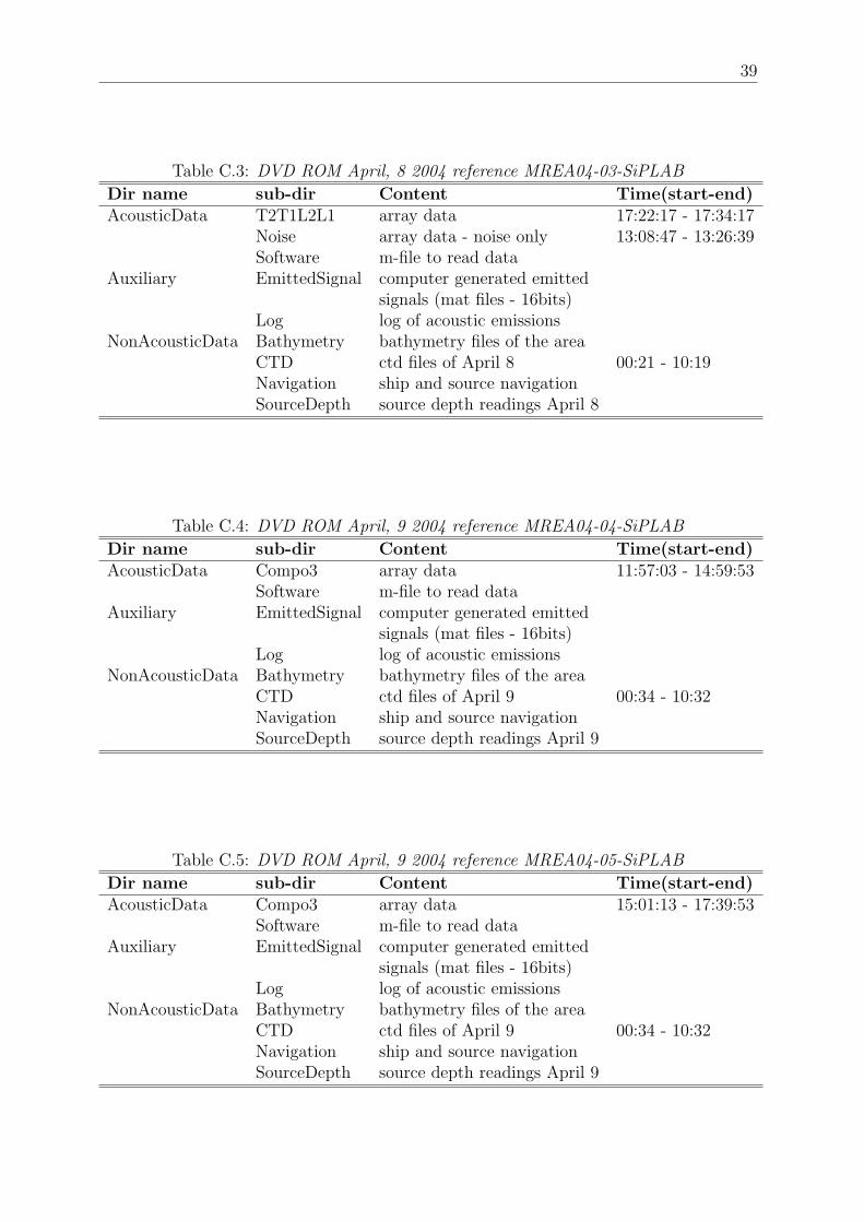
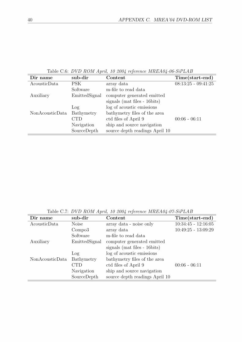
The acoustic data gathered with the Acoustic-Oceanographic buoy as well as file logs andauxiliary reading files are contained in seven DVD-ROMs, attached to the back cover ofthis report. Tables C.1 to C.7 list and describe all DVD-ROM files and directories.

Table C.1: DVD ROM April, 7 2004 reference MREA04-01-SiPLAB

Dir name sub-dir Content Time(start-end)AcousticData Noise array data - noise only 12:55:51-13:27:26

T2T1L2L1 array data 13:28:46 - 16:59:26Software m-file to read data

Auxiliary EmittedSignal computer generated emittedsignals (mat files - 16bits)

Log log of acoustic emissionsNonAcousticData Bathymetry bathymetry files of the area

CTD ctd files of April 7 18:17 - 23:57Navigation ship and source navigationSourceDepth source depth readings April 7


Dir name sub-dir Content Time(start-end)AcousticData T2T1L2L1 array data 13:27:59 - 17:20:57

Software m-file to read dataAuxiliary EmittedSignal computer generated emitted

signals (mat files - 16bits)Log log of acoustic emissions

NonAcousticData Bathymetry bathymetry files of the areaCTD ctd files of April 8 00:21 - 10:19Navigation ship and source navigationSourceDepth source depth readings April 8

38

39


Dir name sub-dir Content Time(start-end)AcousticData T2T1L2L1 array data 17:22:17 - 17:34:17

Noise array data - noise only 13:08:47 - 13:26:39Software m-file to read data





Dir name sub-dir Content Time(start-end)AcousticData Compo3 array data 11:57:03 - 14:59:53





Dir name sub-dir Content Time(start-end)AcousticData Compo3 array data 15:01:13 - 17:39:53




40 APPENDIX C. MREA’04 DVD-ROM LIST


Dir name sub-dir Content Time(start-end)AcousticData PSK array data 08:13:25 - 09:41:25





Dir name sub-dir Content Time(start-end)AcousticData Noise array data - noise only 10:34:45 - 12:16:05

Compo3 array data 10:49:25 - 13:09:29Software m-file to read data




acoustic maritime rapid environmental assessment during ...w3.ualg.pt/~sjesus/pubs/b21.pdf ·...

Documents