acquisition and processing strategies for 3d georadar ...lewebb/ccli/various papers/heincke et al...

GEOPHYSICS, VOL. 70, NO. 6 (NOVEMBER-DECEMBER 2005); P. K53–K61, 15 FIGS., 1 TABLE.10.1190/1.2122414

Acquisition and processing strategies for 3D georadar surveying a regioncharacterized by rugged topography

Bjoern Heincke1, Alan G. Green1, Jan van der Kruk1, and Heinrich Horstmeyer1

ABSTRACT

Efficiently performing 3D ground-penetrating radar(GPR or georadar) surveys across rugged terrain andthen processing the resultant data are challenging tasks.Conventional approaches using unconnected GPR andtopographic surveying equipment are excessively timeconsuming for such environments, and special migra-tion schemes may be required to produce meaningfulimages. We have collected GPR data across an unsta-ble craggy mountain slope in the Swiss Alps using anovel acquisition system that records GPR and coinci-dent coordinate information simultaneously. Undulat-ing topography (dips of 8◦ to 16◦) and boulders withdiameters up to about 2 m complicated the field cam-paign. After standard processing, the data were foundto be plagued by time shifts associated with minor coor-dinate inaccuracies, uneven antenna-ground coupling,and numerous small gaps in data coverage. These prob-lems were resolved by passing the data sequentiallythrough an adaptive f -xy deconvolution routine andf -kx and f -ky filters. This filtering also reduced inco-herent noise. Finally, the data were migrated using a3D algorithm that accounted for the undulating topog-raphy. The nonmigrated and migrated images containedgently and moderately dipping reflections from litholog-ical boundaries and actively opening fracture zones. Asuite of prominent diffraction patterns was generated ata steeply dipping fracture zone that projected to the sur-face. Through this case history we introduce a generalstrategy for 3D GPR studies of topographically ruggedland.

INTRODUCTION

Over the past two decades, surface ground-penetratingradar (GPR or georadar) methods have been widely used to

Manuscript received by the Editor May 7, 2004; revised manuscript received September 17, 2004; published online October 21, 2005.1Swiss Federal Institute of Technology, Institute of Geophysics, ETH-Honggerberg, CH-8093, Zurich, Switzerland. E-mail: [email protected];

[email protected], [email protected]; [email protected]© 2005 Society of Exploration Geophysicists. All rights reserved.

characterize the shallow subsurface to depths of 10 to 50 m.Under favorable conditions, these methods can provide high-resolution structural information in a nondestructive and cost-effective manner. Until about 10 years ago, surface GPR stud-ies were based on sparse 2D profiles. More recently, theyhave been extended to three dimensions, thus allowing highlyheterogeneous structures to be imaged accurately for strati-graphic studies (Beres et al., 1995), for the detection of frac-tures and faults in crystalline rock (Grasmueck and Green,1996), for archaeological surveys (Pipan et al., 1999), and forpaleoseismic investigations (Gross et al., 2002, 2004).

Most 3D GPR data sets have been recorded across topo-graphically flat or gently dipping smooth surfaces. To ourknowledge, none have been collected across topographicallyrugged terrain because of technical reasons; conventional pro-cedures that involve recording GPR data and coordinate in-formation separately are too time consuming for this purpose,and there is no commercially available software for correctlymigrating shallow-wavefield data recorded on undulating sur-faces.

To address these issues, we present data acquisition andprocessing strategies used for 3D GPR surveys in an unsta-ble rugged mountainside that is certain to produce a majorrockslide. The survey was part of a large, multidisciplinary re-search project designed to investigate sliding processes withincrystalline rock and thus to derive a better understanding ofrock failure mechanisms (Willenberg et al., 2002). The pur-pose of the GPR survey was to supply information on the dis-tribution and orientation of fracture zones to approximately40 m depth.

We begin by describing the survey location and our data-acquisition strategy, which involves using a GPR system thatrecords GPR traces and corresponding coordinates simulta-neously. The data processing is complicated by inaccurate co-ordinates in the vicinity of abrupt topographic discontinuities,changes in signal character created by antenna-ground cou-pling variations, and unavoidable data gaps associated withlarge boulders and undulating topography. To suppress these

K53

Downloaded 24 Apr 2009 to 132.198.136.75. Redistribution subject to SEG license or copyright; see Terms of Use at http://segdl.org/

K54 Heincke et al.

negative effects and improve the general quality of the im-ages, a combination of f -xy deconvolution and low-pass spa-tial filtering proves to be effective. A 3D version of Lehmannand Green’s (2000) topographic migration algorithm is thenused to generate representative images of the subsurface. Fi-nally, the shallow fracture distribution is illustrated on verticalsections and horizontal slices extracted from the nonmigratedand migrated 3D data volumes.

SURVEY SITE

The Randa investigation site is situated on a Swiss Alpinemountainside at an altitude of 2350 m, immediately above a1-km-high scarp that resulted from a 30 million-m3 rockslidethat blocked the only land route through the Matter Valley toZermatt in 1991 (Figure 1). Shortly after this event, a 100 ×150 m area of the rock mass above the scarp became unstable.This mass is moving centimeters per year in the direction ofthe 1991 rockslide scarp (Willenberg et al., 2002), such thatopen fractures are now visible at the surface (see Figure 2c).

Our GPR data were recorded across two overlapping sur-vey areas, A1 and A2 (40 × 35 m and 22 × 22 m, respectively),located on a natural terrace about 50 m from the 1991 rock-slide scarp (Figure 2a). The site is covered with low-lying veg-etation and a thin soil layer with a maximum thickness of a fewmeters, typical of Alpine pastures. Isolated boulders (e.g., Iand II in Figures 2a and 2b) with diameters up to 2 m are scat-tered across survey area A1. Although the general slope of themountainside is easterly directed, the rugged and craggy ter-

Figure 1. Photograph of the 1991 Randa rockslide in the SwissAlps (courtesy Heike Willenberg). The investigation site is lo-cated immediately above a rockslide scarp at an altitude of2350 m. The inset locates the site in southern Switzerland.

rain of the GPR survey site dips 8◦ to 16◦ in a southwesterlydirection.

The foliation of the crystalline rock mass, which comprisesa complex mixture of gneisses, schists, amphibolites, andgranitic intrusions (Willenberg et al., 2002), dips roughly 25◦

west-southwest. Along the eastern edges of the survey areas,the outcropping crystalline basement steps approximately 8 mdown to the next terrace (Figure 2a). One open fracture zone,z1 (Figure 2c), and two surface lineaments that likely definefracture zones, z2 and z3, occur within or just outside the sur-vey areas (Figure 2a). Debris and overburden made it difficultto determine the full extent and dips of the fracture zones fromsurface observations.

DATA ACQUISITION

We used Lehmann and Green’s (1999) acquisition system tocollect the GPR and topographic data. It included a standardpulse EKKO 100A GPR unit, a Leica TCA 1800 self-trackingtheodolite, and two field laptop computers (Figure 3).

Recording parameters

Unshielded 100-MHz transmitter and receiver antennasseparated by 1.0-m and a 2.15-m mast holding the theodolitetarget prism were mounted on a sled. The long mast ensured

Figure 2. Photographs of the investigation site. (a) Viewedfrom the west, the dashed black lines outline the 3D GPRsurvey areas A1 and A2. The solid red line delineates surfacefracture z1. Surface lineaments that may delineate fracturesare shown by dashed red lines. Numerous large boulders (di-ameters of 1 to 2 m) are scattered across area A1, the largestof which are marked I and II. Crystalline basement rocks out-crop along the eastern edges of the survey areas. (b) Viewedfrom the south, highly uneven topographic relief and numer-ous boulders complicate the 3D GPR data acquisition. I andII are as for (a). (c) Surface fracture z1.


3D Georadar Surveying Rugged Terrain K55

continuous line of sight between the theodolite and prism inregions with large boulders and other topographic undula-tions. Fiber-optic cables connected all components of the ac-quisition system. While towing the sled, the laser theodoliteautomatically followed the prism, such that the GPR tracesand coordinates of the prism were recorded simultaneously.

The same acquisition parameters were used for the two sur-veys, which were conducted two months apart. Since the rockmass was generally dry (no standing water was observed in anearby 120-m-deep borehole), the recording conditions werevery similar for the two surveys. To take advantage of the ap-proximately 40-m depth penetration offered by the dry-rockenvironment, a long 1050.4-ns recording window was adopted(Table 1). Each recorded trace was the result of verticallystacking 32 individual traces.

To ensure the nonaliased recording of steeply dippingevents, the spacing �d between traces in common-offset datashould be

�d ≤ vmin

4fmax sin amax, (1)

where fmax is the maximum dominant signal frequency, vmin

is the lowest expected GPR velocity, and amax is the steepestexpected reflector dip. Dominant signal frequencies at Randa

Table 1. Acquisition parameters for the 3D GPR surveys A1and A2.

Parameter Value

Nominal antenna frequency 100 MHzRecording length 1050.4 nsSampling interval 0.8 nsVertical stack 32Nominal spacing in x-direction (crossline) ∼0.2 mNominal spacing in y-direction (inline) ∼0.25 mEstimated coordinate x ∼ 0.03 m

accuracy (except for regions y ∼ 0.04 mcovered by large boulders) z ∼ 0.01 m

Figure 3. Principal elements of the semiautomated GPR dataacquisition system, which includes a commercial GPR unit, aself-tracking laser theodolite with automatic target recogni-tion capabilities, and two field laptop computers for recordingthe GPR and positional information (modified from Lehmannand Green, 1999).

are <80 MHz when using the 100-MHz antennas, and veloci-ties are approximately 0.115 m/ns (estimated from common-midpoint measurements and georadar recordings betweennearby boreholes). Based on these values, equation 1 suggeststhat 0.25-m sampling intervals in the crossline (x) and inline(y) directions should allow features with arbitrary strikes anddips to be recorded.

The 3D data were collected along approximately parallelstraight lines as far as the rugged topography would allow(e.g., it was not possible to survey across boulder I, shownin Figure 2b). Because of the long recording times and highdegree of vertical stacking, the GPR acquisition unit couldonly record roughly two stacked traces per second. To pro-vide GPR traces every 0.25 m and coordinates every 0.025 malong the y-direction, the sled was moved at a slow maximumrate of about 0.5 m/s. Sampling in the x-direction varied from0.15 to 0.25 m.

Problems associated with data acquisition

Accurate coordinates are critical for reliable processing andinterpretation of 3D GPR data. For self-tracking theodo-lites, accuracy of the changing coordinates depends primar-ily on the angular velocity of the rotating theodolite head,which is a function of target prism velocity and distance be-tween the theodolite head and prism. For the slow surveyingpace across the Randa site, the self-tracking theodolite pro-vided prism coordinates that were mostly accurate to about0.03 m (Lehmann and Green, 1999). Unavoidable suddentilting of the mast as the relatively heavy sled was movedacross major topographic discontinuities (e.g., large boulders;Figure 4) resulted in lower coordinate accuracy, particularly inthe z-direction. Tilting of the antennas and associated changesin their height above the ground also produced irregularantenna-ground coupling conditions and associated variationsin the antenna radiation patterns and GPR pulse shapes.

DATA PROCESSING

Our scheme for processing the coordinate and GPR data isoutlined in Figure 5. Processes influenced by topography arehighlighted in the gray boxes.

Figure 4. Diagram illustrating the misalignment of the targetprism and the center of the antennas when the sled is pulledacross boulders and other major surface undulations.


K56 Heincke et al.

Topographic model and antenna coordinate errors

The coordinates of the target prism provided by the theodo-lite are shown in Figure 6a. Gaps in coverage were caused byrapid tilting of the prism mast at abrupt topographic discon-tinuities. To determine the coordinates of the center pointsbetween the antennas at the base of the mast, which were re-quired for data processing, we used Lehmann and Green’s(1999) polynomial-fitting scheme. This scheme yielded moreevenly distributed coordinates with fewer and smallergaps than the distribution of prism coordinates (compareFigures 6a and 6b). By combining the recording times of thecoordinates with those of the GPR data, it was then possi-ble to assign a coordinate to each GPR trace (Figure 6c).According to simulations described by Lehmann and Green(1999), postacquisition processing of the coordinate informa-tion added errors of about 0.01 m, which, when combined withthe nearly 0.03-m prism coordinate inaccuracy, resulted in aroughly 0.04-m total coordinate error for most GPR traces.Undoubtedly, much larger errors occurred in the vicinity ofboulders and other abrupt topographic variations.

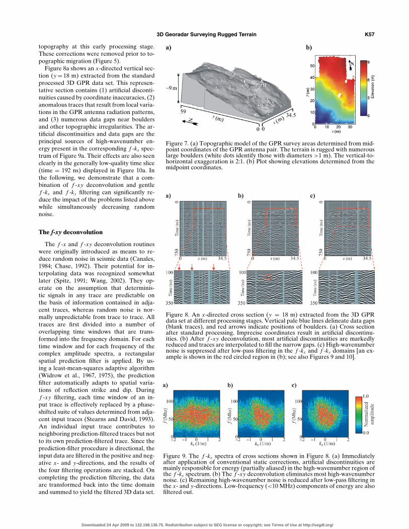
A perspective view of the topography represented by thecoordinates in Figures 6b and 6c is displayed in Figure 7.White dots identify boulders. The dip varies from 8◦ to16◦, except near and across large boulders where local dipsreach 40◦.

Creating a regular grid of GPR data

Since many processing methods require regularly orderedspatial data, the GPR data were resampled onto a regulargrid with points separated by 0.25 m in the x- and y-directions(Figure 6d). Only the nearest traces to the gridpoints were in-corporated in the final data set. If two or more traces wererecorded at the same short distance from a gridpoint (to within0.01 m), they were stacked together. If no trace was recorded

Figure 5. Processing sequence applied to the 3D GPR datasets. Operations influenced by topography are contained ingray boxes.

within 0.225 m of a gridpoint, a blank trace was inserted at thatpoint.

Standard processing

After applying a filter to remove low-frequency wow(Gerlitz et al., 1993) and aligning first arrivals, each GPRtrace was subjected to an exponential gain function that in-creased the amplitudes of later events relative to those of ear-lier ones (Figure 5). The traces were then passed through time-variant, low-pass frequency filters that reduced the randomnoise; with increasing traveltime, the cutoff frequency was de-creased from 120 to 75 MHz to account for the stronger at-tenuation of the higher-frequency components of the signal.To determine the continuity of reflections and diffractions, itwas necessary to minimize the effects of topography by ap-plying provisional static corrections (using a constant velocityv = 0.115 m/ns). Although standard topographic static correc-tions are less than ideal in GPR applications (Lehmann andGreen, 2000), it was necessary to account approximately for

Figure 6. (a) Positions of target prism measured by the theodo-lite. Because the mast carrying the target prism tilts whenmoved across boulders (Figure 4), gaps are present in the po-sitional data. (b) Midpoint positions of the sled, obtained afterremoving the influence of the mast length. (c) Midpoint posi-tions of GPR transmitter-receiver antenna pairs. (d) Equallyspaced 0.25 × 0.25-m gridpoints to which traces are assigned.



topography at this early processing stage.These corrections were removed prior to to-pographic migration (Figure 5).

Figure 8a shows an x-directed vertical sec-tion (y = 18 m) extracted from the standardprocessed 3D GPR data set. This represen-tative section contains (1) artificial disconti-nuities caused by coordinate inaccuracies, (2)anomalous traces that result from local varia-tions in the GPR antenna radiation patterns,and (3) numerous data gaps near bouldersand other topographic irregularities. The ar-tificial discontinuities and data gaps are theprincipal sources of high-wavenumber en-ergy present in the corresponding f -kx spec-trum of Figure 9a. Their effects are also seenclearly in the generally low-quality time slice(time = 192 ns) displayed in Figure 10a. Inthe following, we demonstrate that a com-bination of f -xy deconvolution and gentlef -kx and f -ky filtering can significantly re-duce the impact of the problems listed abovewhile simultaneously decreasing randomnoise.

The f-xy deconvolution

The f -x and f -xy deconvolution routineswere originally introduced as means to re-duce random noise in seismic data (Canales,1984; Chase, 1992). Their potential for in-terpolating data was recognized somewhatlater (Spitz, 1991; Wang, 2002). They op-erate on the assumption that determinis-tic signals in any trace are predictable onthe basis of information contained in adja-cent traces, whereas random noise is nor-mally unpredictable from trace to trace. Alltraces are first divided into a number ofoverlapping time windows that are trans-formed into the frequency domain. For eachtime window and for each frequency of thecomplex amplitude spectra, a rectangularspatial prediction filter is applied. By us-ing a least-mean-squares adaptive algorithm(Widrow et al., 1967, 1975), the predictionfilter automatically adapts to spatial varia-tions of reflection strike and dip. Duringf -xy filtering, each time window of an in-put trace is effectively replaced by a phase-shifted suite of values determined from adja-cent input traces (Stearns and David, 1993).An individual input trace contributes toneighboring prediction-filtered traces but notto its own prediction-filtered trace. Since theprediction-filter procedure is directional, theinput data are filtered in the positive and neg-ative x- and y-directions, and the results ofthe four filtering operations are stacked. Oncompleting the prediction filtering, the dataare transformed back into the time domainand summed to yield the filtered 3D data set.

Figure 7. (a) Topographic model of the GPR survey areas determined from mid-point coordinates of the GPR antenna pair. The terrain is rugged with numerouslarge boulders (white dots identify those with diameters >1 m). The vertical-to-horizontal exaggeration is 2:1. (b) Plot showing elevations determined from themidpoint coordinates.

Figure 8. An x-directed cross section (y = 18 m) extracted from the 3D GPRdata set at different processing stages. Vertical pale blue lines delineate data gaps(blank traces), and red arrows indicate positions of boulders. (a) Cross sectionafter standard processing. Imprecise coordinates result in artificial discontinu-ities. (b) After f -xy deconvolution, most artificial discontinuities are markedlyreduced and traces are interpolated to fill the narrow gaps. (c) High-wavenumbernoise is suppressed after low-pass filtering in the f -kx and f -ky domains [an ex-ample is shown in the red circled region in (b); see also Figures 9 and 10].

Figure 9. The f -kx spectra of cross sections shown in Figure 8. (a) Immediatelyafter application of conventional static corrections, artificial discontinuities aremainly responsible for energy (partially aliased) in the high-wavenumber region ofthe f -kx spectrum. (b) The f -xy deconvolution eliminates most high-wavenumbernoise. (c) Remaining high-wavenumber noise is reduced after low-pass filtering inthe x- and y-directions. Low-frequency (<10 MHz) components of energy are alsofiltered out.


K58 Heincke et al.

From the above description, it is apparent that the effectsof small numbers of anomalous traces are suppressed and thatsmall numbers of blank traces are replaced by interpolatedones. Gross et al. (2002, 2004) use f -xy deconvolution to re-duce random noise in 3D GPR data, but to our knowledge itsefficacy in compensating for anomalous time shifts and inter-polating missing GPR traces has not been demonstrated (seeAppendix A for results of applying f -xy deconvolution to syn-thetic 3D GPR data characterized by erroneous time shiftsand missing traces).

Results of f-xy deconvolution and f-k filtering

We selected (1) a short 3 × 3 trace filter to ensure thatcurved events (e.g., diffractions) and short reflections werelargely preserved and (2) a short 100-ns time window to limitthe number of differently oriented structures that had to behandled by the f -xy deconvolution algorithm. After f -xy de-convolution, the continuity of reflections and diffractions wasmarkedly enhanced. For example, many of the artificial dis-continuities were noticeably suppressed in the equivalent f -xy deconvolved vertical section of Figure 8b and time sliceof Figure 10b, and most of the blank traces were replaced byappropriately interpolated ones. Even though completely un-correlated noise was reduced after f -xy deconvolution, high-wavenumber noise that correlated over several traces was ei-

Figure 10. Time slices at t = 192 ns at the same processingstages represented by Figures 8 and 9. Data gaps are delin-eated in light blue-gray. (a) Time slice immediately after ap-plication of static corrections has numerous blank traces andartificial discontinuities that result in a generally low-qualityimage. (b) After f -xy deconvolution, most artificial discon-tinuities are suppressed and traces are interpolated to fill thenarrow gaps. Unfortunately, an artificial checkerboard patternis visible after this processing step. (c) Application of f -kx andf -ky filters considerably reduces the effects of the checker-board pattern. At this stage, filtered traces that have fewerthan three neighboring traces are deleted.

ther only partly removed or marginally enhanced as a resultof the short filter length. This is clear from the noise in theregion of Figure 8b, delineated by the red circle, and the ar-tificial checkerboard pattern in Figure 10b. Nevertheless, f -xy deconvolution markedly decreased the energy in the high-wavenumber parts of the f -k spectra (e.g., Figure 9b).

To remove the remaining high-wavenumber noise, wepassed the f -xy deconvolved data through low-pass spatial fil-ters in the f -kx and f -ky domains (Figure 5). Subsequently,all originally blank traces that had fewer than three neigh-boring traces before f -xy deconvolution were replaced byblank traces. Figures 8c, 9c, and 10c demonstrate the efficiencyof the low-pass spatial filtering in eliminating the remaininghigh-wavenumber noise; the high-wavenumber jitter is not ob-served in Figure 8c, and the checkerboard pattern is not seenin Figure 10c.

Three-dimensional topographic migration

Synthetic studies have demonstrated the inadequacies ofconventional GPR migration procedures when surface dipsare much greater than 6◦ and/or short-wavelength topographicrelief as small as 1 to 2 m is present (Lehmann and Green,2000). After removing the provisional static corrections (Fig-ure 5), we used a modified 3D version of Lehmann andGreen’s (2000) topographic migration algorithm to migratethe GPR data directly from the irregular acquisition surfaceusing a constant 0.115-m/ns velocity.

Effects of f-xy deconvolution andf-k filtering on GPR images

Comparison of the unmigrated images of Figures 8c and10c with those of Figures 8a and 10a demonstrates the sig-nificantly enhanced reflection continuity that results fromf -xy deconvolution and f -k filtering. Equally impressive arethe improvements in the corresponding migrated images (Fig-ure 11). Many reflections in the migrated unfiltered data areinterrupted by artificial vertical offsets, and numerous migra-tion smiles result from the poor quality of the input data (Fig-ures 11a and 11c). In contrast, reflections in the migrated fil-tered data are relatively continuous and the smiles are barelyperceptible (Figures 11b and 11d).

INTERPRETATION

Typical vertical and horizontal sections extracted from thefinal premigrated and migrated GPR data are displayed in Fig-ures 12 and 13. We focus our interpretation on the strongestreflections and diffractions, A–D. The very shallow reflectionA dips 15◦ to 18◦ to the southwest. Since it approaches thesurface along the eastern and northern edges of the surveyarea where the crystalline basement outcrops (Figure 2a), it isprobably generated at the overburden/rock boundary. If thisinterpretation is correct, then the overburden is thickest atabout 4 m under the southwestern corner of survey area A1.

High-amplitude reflection B is relatively continuous overa 1500 m2 area. It dips approximately 25◦ to the south-west, roughly parallel to the principal bedrock foliation. Likereflection A, it approaches the surface at the eastern and



Figure 11. (a, b) As for Figures 8a and 8c, respectively, but af-ter application of 3D topographic migration. (c, d) Same as (a)and (b) except for selected reflections that are more continu-ous as a result of f -xy deconvolution and f -kx and f -ky filter-ing. These reflections are outlined in red ovals; reflections withnoise removed by the same process are outlined in dashed redovals.

northern edges of the survey area, and it can be traced to amaximum depth of about 11.5 m. It may originate from a sig-nificant change in lithology or a foliation-controlled fracturezone.

Reflection C, best observed on the nonmigrated images ofFigure 12, dips 32◦ to 40◦ eastward over the whole length ofsurvey area A1 near its western edge. It projects to the surfacelocation of the lineament that defines the probable fracturezone z2 (Figure 2a).

Diffraction patterns D appear at different depths withinthe southern part of the nonmigrated data volume (e.g., Fig-ure 12). After migration they collapse to a steeply dipping se-ries of point or line sources (e.g., Figure 13). We suspect theyare created along the edges of a steeply dipping fracture zonez3 (Figures 2a and 13g).

Although z1 is the most prominent fracture zone withinsurveyed areas A1 and A2, any reflections or diffractionsfrom it are not obvious in Figures 12 and 13. A lackof reflections is not unexpected because neither the radia-tion characteristics of the unshielded dipole-type antennasnor the survey geometry is favorable for imaging a north-northwest steeply dipping feature at the location of z1. Wesuspect that high background noise and destructive interfer-ence mask any associated diffraction patterns in Figures 12and 13.

Figure 12. (a) Two intersecting cross sections and one time slice extracted from the final nonmigrated data. (b, c)Cross sections in the x- and y-directions. (d–g) Time slices. The surface is delineated by dashed lines in (a)–(c).Several significant reflections (e.g., A, B, and C) and diffractions (e.g., D) are visible.


K60 Heincke et al.

Figure 13. As for Figure 12 after topographic migration. (g) The positions of surface features z1, z2, and z3are delineated.

SUMMARY AND CONCLUSIONS

We have described efficient acquisition and processingmethods for 3D GPR data surveying a terrain distinguished byrugged topography. Our acquisition system allows GPR dataand corresponding coordinates to be recorded simultaneouslyacross a highly fractured and craggy rock mass. Most coordi-nates were determined to better than 0.04 m. In the vicinityof large boulders and other abrupt topographic discontinu-ities, the data were affected by markedly larger coordinate in-accuracies, varying antenna-ground coupling conditions, anddata gaps (i.e., nearly 23% blank traces). These problems weregreatly reduced or eliminated by f -xy deconvolving and f -kfiltering the data. The final critical processing step involvedpassing the data through a 3D topographic migration scheme.

Members of our group have recently tested a GPR data-acquisition system that includes a standard GPR unit coupledto a high-quality differential GPS instrument. The advantagesand disadvantages of this combination are comparable to thesystem used for the Randa survey. In contrast to the theodo-lite, the coordinate accuracy provided by the differential GPSdid not decrease significantly with acquisition speed but in-stead depended strongly on the available satellite coverage.

Regardless of the acquisition system used, our resultsdemonstrate that it is possible to record unaliased 3D GPRdata across highly undulating ground, thus allowing di-verse complex and undulating landscapes (e.g., archaeolog-ical mounds, sand dunes, rock glaciers, narrow valleys, andhilly and mountainous regions) to be investigated in a cost-effective manner. As for any georadar survey, the need forrelatively low-conductive near-surface material is the primarylimitation.

The processing of GPR and coordinate data collected acrossrugged terrain is quite complicated, requiring the applica-tion of nonstandard procedures. When working in such en-vironments and under time constraints, coordinate inaccu-racies, uneven antenna-ground coupling, and data gaps areinevitable. Various types of multichannel filtering may helpresolve these problems. Whereas f -xy deconvolution is rela-tively robust, f -k filtering needs to be applied with care (nar-row f -k filters can produce artifacts). For reliable GPR imag-ing of structures below rugged landscapes, the application ofsome form of topographic migration is essential.

ACKNOWLEDGMENTS

We appreciate the advice and suggestions provided by MarkGrasmueck, Ralf Gross, Frank Lehmann, and various person-nel at Landmark Graphics Corporation. We thank BernhardLampe, Martin Musil, and Anya Seward for their enthusiastichelp in the field and Hansruedi Maurer, Tom Spillmann, ErikEberhardt, Simon Low, and Heike Willenberg for their coop-eration in this interdisciplinary project. This research projectwas supported financially by a grant from the Swiss NationalScience Foundation.

APPENDIX A

EFFICACY OF f-xy DECONVOLUTIONIN MINIMIZING ANOMALOUS TIME SHIFTS

AND INTERPOLATING TRACES

To investigate the potential of f -xy deconvolution for re-ducing artificial time shifts and interpolating missing traces,numerous tests based on synthetic 3D data sets have been



performed. We present two representative examples fromthese tests. The initial error-free synthetic data set of 21 × 21traces includes a planar reflection (100-MHz Ricker signalwavelet) dipping 1.75 ns/trace in the y-direction. The tracelength is 200 ns and the sample interval is 0.8 ns.

To simulate coordinate errors in rugged terrain, we addGaussian-distributed timing errors to the synthetic traces. The

Figure A-1. (a, c) The y-directed cross sections extractedfrom the synthetic 3D GPR data set containing timing errors.(b, d) Corresponding cross sections after application of f -xydeconvolution (filter length: 3 × 3 traces) to the data.

Figure A-2. (a, c) The y-directed cross sections extracted fromthe synthetic 3D GPR data set containing timing errors andblank traces. (b, d) Corresponding cross sections after appli-cation of f -xy deconvolution (filter length: 3×3 traces) to thedata.

rms difference between reflection times in the erroneous anderror-free data is approximately 1.5 ms. Figure A-1a and cshows the effects of these timing errors on two y-directed sec-tions extracted from the flawed 3D data. Figure A-1b and ddemonstrates that the timing errors are mostly eliminated af-ter f -xy deconvolution. It is notable that the signal charac-ter is not significantly affected by this operation; the meancrosscorrelation coefficient between the f -xy deconvolvedand original error-free data is about 0.95.

Data gaps are simulated by randomly blanking 28.8% of thetraces contained in the already flawed data set (Figure A-2aand c). Application of f -xy deconvolution results in the re-moval of the timing errors and appropriate interpolation ofthe missing traces (Figure A-2b and d). The mean crosscorre-lation coefficient between the f -xy deconvolved and originalerror-free data is a surprisingly high 0.96.

Our extensive tests (only two of which are shown here) havedemonstrated that comparably good f -xy deconvolution re-sults can be expected for data sets plagued by timing errors aslarge as 2.0 ms and with up to 45% missing traces.

REFERENCES

Beres, M., A. G. Green, P. Huggenberger, and H. Horstmeyer, 1995,Detailed 3-D georadar studies of glaciofluvial sediments: Geology,12, 1071–1091.

Canales, L. L., 1984, Random noise reduction: 54th Annual Interna-tional Meeting, SEG, Expanded Abstracts, 525–527.

Chase, M., 1992, Random noise reduction by 3-D spatial predictionfiltering: 62nd Annual International Meeting, SEG, Expanded Ab-stracts, 1151–1152.

Gerlitz, K., M. D. Knoll, G. M. Cross, D. Luzitano, and R. Knight,1993, Processing ground penetrating radar data to improve reso-lution of near-surface targets: Symposium on the Application ofGeophysics to Engineering and Environmental Problems, Environ-mental and Engineering Geophysical Society, Expanded Abstracts,561–574.

Grasmueck, M., and A. G. Green, 1996, 3-D georadar mapping: Look-ing into the subsurface: Environmental Engineering Geoscience, 2,195–200 .

Gross, R., A. G. Green, K. Holliger, H. Horstmeyer, and J. Bald-win, 2002, Shallow geometry and displacements on the San Andreasfault near Point Arena based on trenching and 3-D georadar sur-veying: Geophysical Research Letters, 29, 34-1–34-4.

Gross, R., A. G. Green, H. Horstmeyer, and J.Begg, 2004, Loca-tion and geometry of the Wellington fault (New Zealand) definedby detailed 3-D georadar: Journal of Geophysical Research, 109,B05401.

Lehmann, F., and A. G. Green, 1999, Semiautomated georadar dataacquisition in three dimensions: Geophysics, 64, 719–731.

——, 2000, Topographic migration of georadar data: Implications foracquisition and processing: Geophysics, 65, 836–848.

Pipan, M., L. Baradello, E. Forte, A. Prizzon, and I. Finetti, 1999, 2-Dand 3-D processing and interpretation of multi-fold ground pene-trating radar data: A case history from an archaeological site: Jour-nal of Applied Geophysics, 41, 271–292.

Spitz, S., 1991, Seismic trace interpolation in the f -x domain: Geo-physics, 56, 785–794.

Stearns, S. D., and R. A. David, 1993, Signal processing algorithms inFortran and C: Prentice-Hall, Inc.

Wang, Y., 2002, Seismic trace interpolation in the f -x-y domain: Geo-physics, 67, 1232–1239.

Widrow, B., J. R. Glover Jr., J. M. McCool, J. Kaunitz, C. S. Williams,R. H. Hearn, J. R. Zeidler, E. Dong Jr., and R. C. Goodlin, 1975,Adaptive noise cancelling: Principles and applications: IEEE Pro-ceedings, 63, 1692–1716.

Widrow, B., P. Mantey, L. Griffiths, and B. Goode, 1967, Adaptiveantenna systems: IEEE Proceedings, 55, 2143–2159.

Willenberg, H., T. Spillmann, E. Eberhardt, K. Evans, S. Loew, andH. R. Maurer, 2002, Multidisciplinary monitoring of progressivefailure processes in brittle rock slopes — Concepts and system de-sign: 1st European Conference on Landslides, Expanded Abstracts,477–483.


acquisition and processing strategies for 3d georadar ...lewebb/ccli/various papers/heincke et al...

Documents