Action Selection for Hammer Shots in Curling

Zaheen Farraz Ahmad, Robert C. Holte, Michael BowlingDepartment of Computing Science

University of Alberta{zfahmad, rholte, mbowling}@ualberta.ca

AbstractCurling is an adversarial two-player game with acontinuous state and action space, and stochastictransitions. This paper focuses on one aspect ofthe full game, namely, finding the optimal “ham-mer shot”, which is the last action taken before ascore is tallied. We survey existing methods forfinding an optimal action in a continuous, low-dimensional space with stochastic outcomes, andadapt a method based on Delaunay triangulationto our application. Experiments using our curl-ing physics simulator show that the adapted De-launay triangulation’s shot selection outperformsother algorithms, and with some caveats, exceedsOlympic-level human performance.

1 IntroductionCurling is an Olympic sport played between two teams. Thegame is played in a number of rounds (usually 8 or 10) called“ends”. In each end, teams alternate sliding granite rocksdown a sheet of ice towards a target. When each team hasthrown 8 rocks, the score for that end is determined and addedto the teams’ scores from the previous ends. The rocks arethen removed from the playing surface and the next end be-gins. The team with the highest score after the final end is thewinner.

The last shot of an end, called the “hammer shot”, is of theutmost importance as it heavily influences the score for theend. In this paper, we focus exclusively on the problem ofselecting the hammer shot. This focus removes the need toreason about the opponent, while still leaving the substantialchallenge of efficiently identifying a near-optimal action in acontinuous state and action space with stochastic action out-comes and a highly non-convex scoring function. This workis part of a larger research project that uses search methods toselect all the shots in an end [Yee et al., 2016] and, ultimately,to plan an entire game.

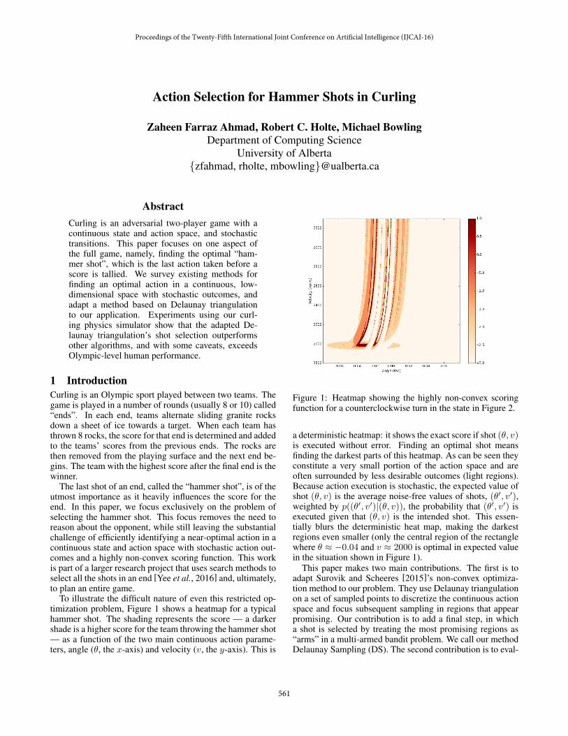
To illustrate the difficult nature of even this restricted op-timization problem, Figure 1 shows a heatmap for a typicalhammer shot. The shading represents the score — a darkershade is a higher score for the team throwing the hammer shot— as a function of the two main continuous action parame-ters, angle (✓, the x-axis) and velocity (v, the y-axis). This is

Figure 1: Heatmap showing the highly non-convex scoringfunction for a counterclockwise turn in the state in Figure 2.

a deterministic heatmap: it shows the exact score if shot (✓, v)is executed without error. Finding an optimal shot meansfinding the darkest parts of this heatmap. As can be seen theyconstitute a very small portion of the action space and areoften surrounded by less desirable outcomes (light regions).Because action execution is stochastic, the expected value ofshot (✓, v) is the average noise-free values of shots, (✓0, v0),weighted by p((✓

0, v

0)|(✓, v)), the probability that (✓0, v0) is

executed given that (✓, v) is the intended shot. This essen-tially blurs the deterministic heat map, making the darkestregions even smaller (only the central region of the rectanglewhere ✓ ⇡ �0.04 and v ⇡ 2000 is optimal in expected valuein the situation shown in Figure 1).

This paper makes two main contributions. The first is toadapt Surovik and Scheeres [2015]’s non-convex optimiza-tion method to our problem. They use Delaunay triangulationon a set of sampled points to discretize the continuous actionspace and focus subsequent sampling in regions that appearpromising. Our contribution is to add a final step, in whicha shot is selected by treating the most promising regions as“arms” in a multi-armed bandit problem. We call our methodDelaunay Sampling (DS). The second contribution is to eval-

Proceedings of the Twenty-Fifth International Joint Conference on Artificial Intelligence (IJCAI-16)

561

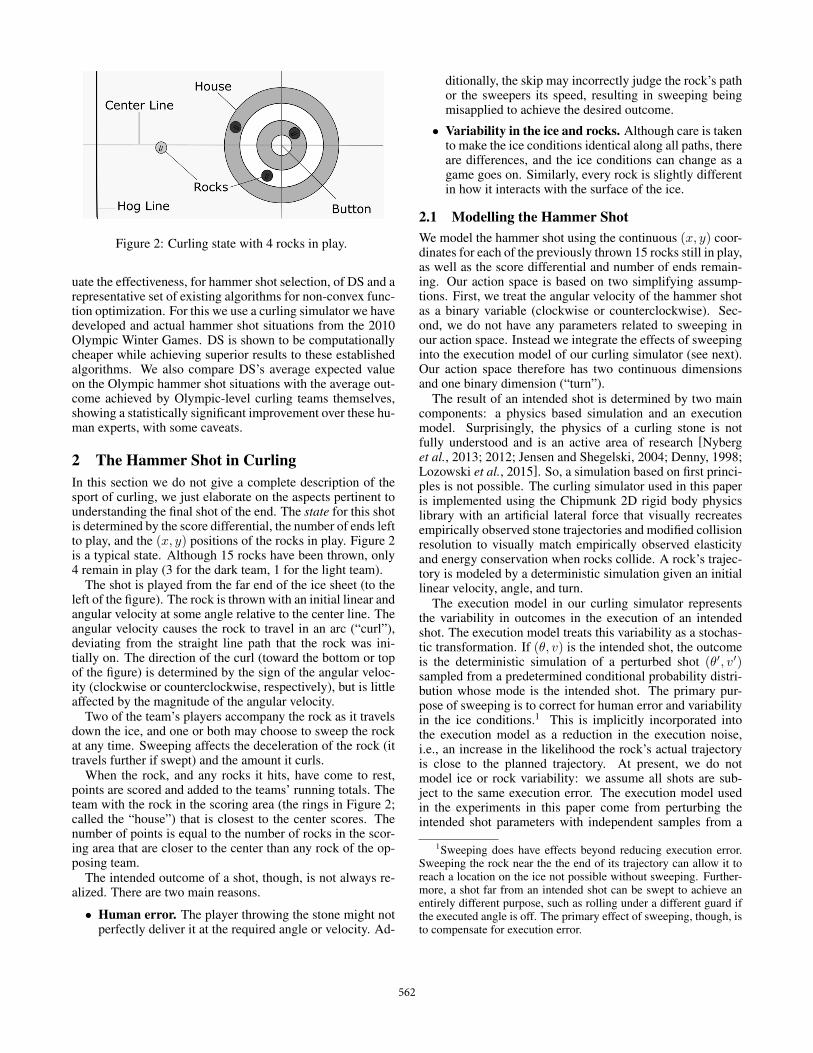
Figure 2: Curling state with 4 rocks in play.

uate the effectiveness, for hammer shot selection, of DS and arepresentative set of existing algorithms for non-convex func-tion optimization. For this we use a curling simulator we havedeveloped and actual hammer shot situations from the 2010Olympic Winter Games. DS is shown to be computationallycheaper while achieving superior results to these establishedalgorithms. We also compare DS’s average expected valueon the Olympic hammer shot situations with the average out-come achieved by Olympic-level curling teams themselves,showing a statistically significant improvement over these hu-man experts, with some caveats.

2 The Hammer Shot in CurlingIn this section we do not give a complete description of thesport of curling, we just elaborate on the aspects pertinent tounderstanding the final shot of the end. The state for this shotis determined by the score differential, the number of ends leftto play, and the (x, y) positions of the rocks in play. Figure 2is a typical state. Although 15 rocks have been thrown, only4 remain in play (3 for the dark team, 1 for the light team).

The shot is played from the far end of the ice sheet (to theleft of the figure). The rock is thrown with an initial linear andangular velocity at some angle relative to the center line. Theangular velocity causes the rock to travel in an arc (“curl”),deviating from the straight line path that the rock was ini-tially on. The direction of the curl (toward the bottom or topof the figure) is determined by the sign of the angular veloc-ity (clockwise or counterclockwise, respectively), but is littleaffected by the magnitude of the angular velocity.

Two of the team’s players accompany the rock as it travelsdown the ice, and one or both may choose to sweep the rockat any time. Sweeping affects the deceleration of the rock (ittravels further if swept) and the amount it curls.

When the rock, and any rocks it hits, have come to rest,points are scored and added to the teams’ running totals. Theteam with the rock in the scoring area (the rings in Figure 2;called the “house”) that is closest to the center scores. Thenumber of points is equal to the number of rocks in the scor-ing area that are closer to the center than any rock of the op-posing team.

The intended outcome of a shot, though, is not always re-alized. There are two main reasons.

• Human error. The player throwing the stone might notperfectly deliver it at the required angle or velocity. Ad-

ditionally, the skip may incorrectly judge the rock’s pathor the sweepers its speed, resulting in sweeping beingmisapplied to achieve the desired outcome.

• Variability in the ice and rocks. Although care is takento make the ice conditions identical along all paths, thereare differences, and the ice conditions can change as agame goes on. Similarly, every rock is slightly differentin how it interacts with the surface of the ice.

2.1 Modelling the Hammer ShotWe model the hammer shot using the continuous (x, y) coor-dinates for each of the previously thrown 15 rocks still in play,as well as the score differential and number of ends remain-ing. Our action space is based on two simplifying assump-tions. First, we treat the angular velocity of the hammer shotas a binary variable (clockwise or counterclockwise). Sec-ond, we do not have any parameters related to sweeping inour action space. Instead we integrate the effects of sweepinginto the execution model of our curling simulator (see next).Our action space therefore has two continuous dimensionsand one binary dimension (“turn”).

The result of an intended shot is determined by two maincomponents: a physics based simulation and an executionmodel. Surprisingly, the physics of a curling stone is notfully understood and is an active area of research [Nyberget al., 2013; 2012; Jensen and Shegelski, 2004; Denny, 1998;Lozowski et al., 2015]. So, a simulation based on first princi-ples is not possible. The curling simulator used in this paperis implemented using the Chipmunk 2D rigid body physicslibrary with an artificial lateral force that visually recreatesempirically observed stone trajectories and modified collisionresolution to visually match empirically observed elasticityand energy conservation when rocks collide. A rock’s trajec-tory is modeled by a deterministic simulation given an initiallinear velocity, angle, and turn.

The execution model in our curling simulator representsthe variability in outcomes in the execution of an intendedshot. The execution model treats this variability as a stochas-tic transformation. If (✓, v) is the intended shot, the outcomeis the deterministic simulation of a perturbed shot (✓

0, v

0)

sampled from a predetermined conditional probability distri-bution whose mode is the intended shot. The primary pur-pose of sweeping is to correct for human error and variabilityin the ice conditions.1 This is implicitly incorporated intothe execution model as a reduction in the execution noise,i.e., an increase in the likelihood the rock’s actual trajectoryis close to the planned trajectory. At present, we do notmodel ice or rock variability: we assume all shots are sub-ject to the same execution error. The execution model usedin the experiments in this paper come from perturbing theintended shot parameters with independent samples from a

1Sweeping does have effects beyond reducing execution error.Sweeping the rock near the the end of its trajectory can allow it toreach a location on the ice not possible without sweeping. Further-more, a shot far from an intended shot can be swept to achieve anentirely different purpose, such as rolling under a different guard ifthe executed angle is off. The primary effect of sweeping, though, isto compensate for execution error.

562

heavy-tailed, zero-mean, Student-t distribution whose param-eters have been tuned to match Olympic-level human ability.

3 Related WorkWe describe the four existing approaches to non-convex opti-mization we explored in this work, as well as work on curlingand the similar game of billiards.

3.1 Continuous BanditsIn the general bandit problem, an agent is presented with a setof arms. Each round, the agent selects an arm and receives areward. The reward received from an arm is an i.i.d. samplefrom the unknown distribution associated with that arm. Theobjective of the agent is to select arms to maximize its cu-mulative reward. Upper Confidence Bounds (UCB) [Auer etal., 2002] is an arm selection policy that associate with eacharm an upper bound on the estimated expected value giventhe entire history of interaction using the following equation:

vi = ri + C

rlogN

ni, (1)

where ri is the average reward observed by the arm i, N isthe total number of samples, ni is the number of times armi was selected, and C is a tunable constant. On each round,the agent chooses an arm i that maximizes vi. The two termsin the upper bound balance between exploiting an action withhigh estimated value and exploring an action with high un-certainty in its estimate.

The continuous bandit problem generalizes this frameworkto continuously parameterized action spaces [Bubeck et al.,2009; Kleinberg, 2004]. The agent is presented with a set ofarms X , which form a topological space (or simply thoughtof as a compact subset of Rn where n is the size of the actionparameterization). On each round, the agent selects a pointx 2 X and receives a reward determined by a randomly sam-pled function from an unknown distribution, which is thenevaluated at x. With some continuity assumptions on themean function of the unknown distribution, one can devisealgorithms that can achieve a similar exploration-exploitationtradeoff as in the finite arm setting.

One such algorithm is Hierarchical Optimistic Optimiza-tion (HOO) [Bubeck et al., 2009]. HOO creates a covertree spanning the action space which successively dividesthe space into smaller sets at each depth. The nodes of thecover tree are treated as arms of a sequential bandit problem.Exploitation is done by traversing down previously-explored,promising nodes to create a finer granularity of estimates. Ex-ploration is performed by sampling nodes higher up in thetree covering regions that have not been sampled adequately.Under certain smoothness assumptions, the average reward ofHOO’s sampled actions converges to the optimal action.

3.2 Gaussian Process OptimizationGaussian Process Optimization (GPO) [Rasmussen, 2006;Snelson and Ghahramani, 2005; Snoek et al., 2012; Lizotteet al., 2007] is based on Gaussian processes, which are priorsover functions, parameterized by a mean function, m(x), anda covariance kernel function, k(x,x0

). Suppose there is an

unknown function f and one is given N observed data points,{xn, yn}Nn=1

, where yn ⇠ N (f(xn), ⌫) with ⌫ being a noiseterm. The posterior distribution on the unknown function f

is also a Gaussian process with a mean and covariance ker-nel function computable in closed form from the data. GPOseeks to find a maximum of an unknown function f throughcarefully choosing new points xn+1

to sample a value basedon the posterior belief from previous samples. The optimalselection mechanism for a non-trivial sampling horizon andprior is intractable. However, good performance can often behad by instead choosing a point that maximizes some acqui-sition function as a proxy objective, e.g., choosing the pointwith the maximum probability of improving on the largestpreviously attained value.

GPO has several drawbacks. As is common with Bayesianmethods, the choice of prior can have a significant impact onits performance. While a parameterized prior can be used andfit to the data, this shifts the problem to selecting hyperparam-eters. The second drawback is computation. Even with workon efficiently approximating the kernel matrix inverse at theheart of Gaussian processes [Snelson and Ghahramani, 2005;Snoek et al., 2012], computation to identify a new samplepoint is still growing with the number of previous samples,which can become intractable when allowing a large numberof samples.

3.3 Particle Swarm OptimizationParticle Swarm Optimization (PSO) [Eberhart and Shi, 2011;Shi and Eberhart, 1998] is a population-based, stochastic ap-proach to optimization. Each particle in the population keepstrack of its own best score and the global best score evalu-ated at each time step. The particles (samples) are initiallyevaluated at uniform random points in the action space. Ateach iteration of the algorithm, the particles take a step towardthe current global best. The step size depends on weight andvelocity parameters, which are decided by the practitioner,and on the particle’s own best score. Unlike HOO and GPO,which make a global convergence guarantee under smooth-ness assumptions, PSO is only expected to converge to a lo-cal optimum, and so results depend on the quality of the initialsampling of points.

3.4 Covariance Matrix Adaptation - EvolutionStrategy

The final optimization method we explore is Covariance Ma-trix Adaption Evolution Strategy (CMA-ES) Evolution strate-gies [Back et al., 1991] are iterative algorithms that attemptto optimize a function by introducing stochastic variationsat each iteration. CMA-ES [Hansen and Ostermeier, 1996;Hansen, 2016] proceeds by drawing a set of samples froman (initially uninformed) multivariate Gaussian. A new mul-tivariate Gaussian is then constructed. The mean is theweighted mean of the sampled points, where higher weightsare given to samples with larger reward values. The covari-ance matrix is modified from the previous covariance so asto encourage high variance in the direction that the mean isobserved to be changing. This procedure is then repeated us-ing the new multivariate Gaussian to sample points. As with

563

PSO, successive generations produced will lead to conver-gence to a local optimum of the function, with no guaranteewith respect to the global optimum.

3.5 Curling and BilliardsPrevious work has been done on developing strategies forcurling in [Yamamoto et al., 2015]. Work in billiards, agame which is similar to curling with continuous actions andstates along with stochastic outcomes, has received some at-tention in the literature [Archibald et al., 2009; Smith, 2007;2006]. However, in all of this work, the authors use do-main knowledge to create a finite set of discrete actions. Thismakes it possible for search to be employed without address-ing the challenges of optimization in continuous settings. Ourwork seeks to forego domain knowledge as much as possible,in favor of a more domain-independent approach.

4 Delaunay SamplingOur Delaunay Sampling (DS) algorithm consists of asampling stage, based on the work of Surovik andScheeres [2015], and a selection stage.

4.1 Sampling with Delaunay TriangulationDS’s first stage proceeds as follows:

1. Sample the (stochastic) objective function at points dis-tributed uniformly over the range of values of the actionparameters.

2. Apply Delaunay triangulation [Lee and Schachter, 1980]to the sampled points to partition the continuous actionspace into a set of disjoint regions.

3. Assign each region a weight, which we discuss below.4. Sample the set of regions with replacement, with the

probability of a region proportional to its weight.5. Each time a region is selected in the previous step, uni-

form randomly sample a point within it and add it to theset of sampled points, with its value sampled from the(stochastic) objective function at that point.

6. Repeat from step 2 for a fixed number (T ) of iterations.

What remains is to specify the weight wi used for region i

in step 3 above. Let t T be the current iteration of thealgorithm, ai refer to the area of region i, and vij refer to theobserved reward of vertex j of region i. We define the weightfor region i as,

wi = a

1�t/Ti ⇥ s

�t/Ti (2)

wheresi = e

maxj(vij), (3)

and � is a tunable parameter that controls the rate of explo-ration. We call si the score of the region since it will be largeif one of the vertices has been observed to result in high re-ward. Note that if ai is large then wi can be large, encourag-ing the algorithm to refine large regions; if si is large then wi

can be large, encouraging the algorithm to focus on regionswith higher observed rewards. As t increases, more weight isput on refining the high-valued regions, since ultimately only

the high-value regions are used in the selection stage of thealgorithm.

In Step 1 triangulations are done separately for each valueof any discrete action parameters (specifically, the binary”turn” parameter in curling). The other steps use the unionof regions from all triangulations. This allows the algorithmto allocate more samples to the most promising discrete pa-rameter values.

4.2 Selection of the Final ActionThis stage chooses the action that will actually be executedusing the following procedure.

1. Assign new weights to the regions,

wi =1

|vij |X

j

vij . (4)

2. Select the k regions with the highest weights.

3. Run ˆ

T iterations of UCB using the chosen regions asthe arms of a bandit. When UCB samples a region, thesample is taken at the region’s incenter, and its valueis a (stochastic) sample of the objective function at thatpoint.

4. Return the incenter of the region that was sampled mostby UCB.

Different weighting functions are used in the two stages be-cause of the different purposes they serve. The first stageis exploratory, trying to find promising regions that are rel-atively small. For this purpose it makes sense to use an op-timistic score for a region. The aim of the second stage isto identify the region with the largest expected value. Forthis purpose it is appropriate to repeatedly sample the pointwithin a region that would actually be returned. In prelimi-nary tests, Delaunay triangulation and UCB performed poorlywhen used by themselves for the entire process. But as wewill see, together they seem to address each others’ weak-nesses.

5 Experimental SetupAs noted in the introduction, we are interested in exploringall of these methods for the problem of selecting a hammershot in curling.

5.1 Objective FunctionWhat objective function do we wish to optimize? The answerthat usually springs to mind is points, i.e. find a shot with themaximum expected point (EP) differential. To see why thisis not ideal, consider choosing the very last shot of a game inwhich the team with the hammer is losing by two points. Sup-pose shot A is 100% guaranteed to score one point and shotB has a 20% chance of scoring 3 points and an 80% chanceof giving up one point. Shot A has a much higher EP thanB (1.0 compared to �0.2) but it has no hope of winning thegame, whereas B will win 20% of the time. B is obviouslythe better choice in this situation. For this reason, we focuson optimizing win percentage (WP), not EP.

564

The only remaining game state variables after the hammershot is thrown is n, the number of ends left to play, and �

the number of points by which the team with the hammer isleading (� is negative if the team with the hammer is losing).We call a pair (n, �) the resulting game state, or g. For ex-ample, if g = (1,�2), WP(g) is the probability of the teamwith hammer winning if it enters the final end down by twopoints. We then fit this WP function to data using 28,000curling games played between 2011 and 2013.2 For the finalend of a game, g = (1, �), we estimated WP(g) using simplefrequency statistics for the final ends from the dataset. Forthe second last end of a game we used the same data to es-timate the transition probabilities from g = (2, �) to a gamestate g

0= (1, �

0) for the final end. This tells how frequently

it happened that the hammer team having a lead of � whenthere were two ends to play was followed by the hammerteam in the final end having a lead of �0. With these transitionprobabilities and the already-computed values of WP((1, �0))for all �0, it is easy to compute WP((2, �)) for all �. Thesame process can then be applied to compute WP((3, �)),WP((4, �)), etc. With WP(n, �) defined for all values of nand �, the “score” we return when a hammer shot with x endsremaining results in a lead of � for the team with the hammerin the next end is WP(x�1, �). This is the objective functionour methods aim to maximize in expectation in selecting thehammer shot.

5.2 Experimental DesignThe data used for our experiments was drawn from the ham-mer shot states captured by hand from the 2010 WinterOlympics men’s and women’s curling competition.3 A set of397 hammer shot states from these logs were used in the pa-rameter sweeps mentioned below. The parameter sweep forDelaunay Sampling (DS) chose a value of 14 for �. A sep-arate set of 515 hammer shot states (the “test states”) fromthese logs were used to evaluate the systems (including thehumans).

For each of the test states, we gave DS a budget of between500 and 3000 samples. This budget includes 100 samples forinitializing the triangulation over each turn, 100 samples periteration of the first stage, and 100 samples for the final UCBstage. After DS selected a shot, 10 outcomes were sampledfrom the simulator, with the outcome’s sample mean used asthe resulting estimate of WP. This procedure was repeated250 times for each test state. The values we report in Table 1are the average over the 2500 evaluations for each test state.

HOO selected a sample by choosing a turn using UCB andthen expanding the cover tree for that turn. We ran HOO for

2Forfeits were treated as transitions to win/loss states. For rarestates, the outcomes used in estimating the transition probabilitiescame from states with a similar score differential (when near the endof the game) or similar number of ends remaining (when far from theend of the game). The data used came from http://curlingzone.com,and included both women’s and men’s tournaments, although almostno difference was observed when restricting to data only from onegender or when including only championship level events.

3The logs do not contain the actual shot played by the humansthey only contained the states before and after the hammer shotswere taken.

250 trials over the test states using the same sampling bud-gets as DS. The parameters for HOO described by Bubecket al. [2009] were set by a parameter sweep to ⇢ =

1p2

,⌫ = 2

p2 and UCB constant C = 0.01.

PSO was tested slightly differently. Since the particlesmove in a continuous space, having a discrete parameter(“turn”) required us to run PSO on each turn separately. Foreach test state, PSO was run using one turn value and then theother with each run being provided the full sampling budget.The best shots found with each turn were compared and theone with the higher average WP was evaluated one final timeto compute its expected WP . This was performed 250 timesfor each test state. PSO’s parameters were set to c

1

= 1.5,c

2

= 1.5, w = 0.7 and 50 particles.We used the BIPOP-CMA-ES [Auger and Hansen, 2009]

version of CMA-ES for our tests. The experimental setupwas the same as for PSO. The parameters for the number ofoffspring and parents were, respectively, � = 4 + 3 log 2 andµ = �/2 with 4 restarts. We set the initial standard deviationto �

0

= 0.25 and normalized the action parameters ✓ and v torange between 0 and 1. The parameters for step-size controland the covariance matrix adaptation were set in accordanceto the values recommended by Hansen [2016].

GPO was tested in a manner similar to PSO. However,since GPO is considerably slower we implemented it withonly a budget size of 250, 500 and 1000 samples per turnwith 50 restarts. We chose the squared-exponential functionas our GP kernel and set the noise variance, �n = 0.01.

To determine if DS’s average WP on the test states wasstatistically significantly different than the average WP of thehumans or other systems tested, we ran a Wilcoxon signed-rank test (WSRT) with one pair of values for each of the 515test states (one of the values was DS’s WP on the state, theother was the WP of the system DS was being comparedto). Unless otherwise noted, WSRT produced p-values suf-ficiently small to conclude with greater than 99% confidencethat DS’s superior average WP (for any specific sample bud-get) is not due to chance.

6 Results and EvaluationTable 1 shows the performance (WP) on the test states of theoptimization methods in our study. For any given sample bud-get, DS’s WP was significantly better than that of any othersystems tested. HOO performed worse than DS for smallersample budgets because it was slower to build its cover treedeep enough in the more promising parts of the action spaceto accurately locate the best shots. Its peformance growscloser to DS’s as the sample budget increases. PSO’s WPchanged very little as its sample budget increased. We con-jecture this is because good shots are quite rare, so PSO’sinitial, random sample of a noisy fucntion may not containa strong signal to draw the particles towards a global opti-mum. PSO also tends to converge to suboptimal local optima.CMA-ES also suffers from convergence to suboptimal localoptima. GPO tended to take many samples in the large re-gions where the function has a minimum value (the lightestregions in Figure 1). We believe that given a more generoussampling budget, it would eventually find better shots, but its

565

DS Budget DS HOO PSO CMA GPO500 0.4956 0.4273 0.4853 0.4932 0.48571000 0.5203 0.4787 0.4856 0.4958 0.48681500 0.5277 0.4968 0.4858 0.4954 -2000 0.5310 0.5115 0.4849 0.4933 0.48672500 0.5331 0.5176 0.4858 0.4954 -3000 0.5343 0.5212 0.4854 0.4948 -

Table 1: Average WP for different sample budgets.

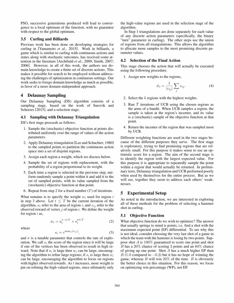
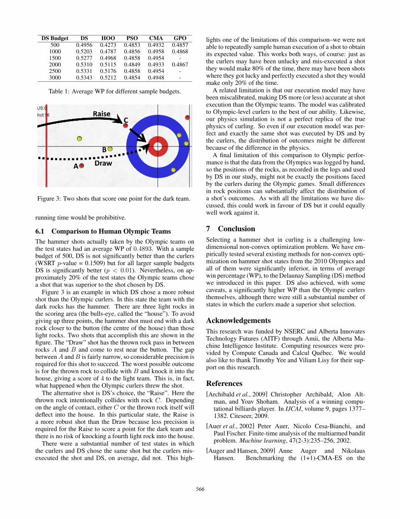
Figure 3: Two shots that score one point for the dark team.

running time would be prohibitive.

6.1 Comparison to Human Olympic TeamsThe hammer shots actually taken by the Olympic teams onthe test states had an average WP of 0.4893. With a samplebudget of 500, DS is not significantly better than the curlers(WSRT p-value = 0.1509) but for all larger sample budgetsDS is significantly better (p < 0.01). Nevertheless, on ap-proximately 20% of the test states the Olympic teams chosea shot that was superior to the shot chosen by DS.

Figure 3 is an example in which DS chose a more robustshot than the Olympic curlers. In this state the team with thedark rocks has the hammer. There are three light rocks inthe scoring area (the bulls-eye, called the “house”). To avoidgiving up three points, the hammer shot must end with a darkrock closer to the button (the centre of the house) than thoselight rocks. Two shots that accomplish this are shown in thefigure. The “Draw” shot has the thrown rock pass in betweenrocks A and B and come to rest near the button. The gapbetween A and B is fairly narrow, so considerable precision isrequired for this shot to succeed. The worst possible outcomeis for the thrown rock to collide with B and knock it into thehouse, giving a score of 4 to the light team. This is, in fact,what happened when the Olympic curlers threw the shot.

The alternative shot is DS’s choice, the “Raise”. Here thethrown rock intentionally collides with rock C. Dependingon the angle of contact, either C or the thrown rock itself willdeflect into the house. In this particular state, the Raise isa more robust shot than the Draw because less precision isrequired for the Raise to score a point for the dark team andthere is no risk of knocking a fourth light rock into the house.

There were a substantial number of test states in whichthe curlers and DS chose the same shot but the curlers mis-executed the shot and DS, on average, did not. This high-

lights one of the limitations of this comparison–we were notable to repeatedly sample human execution of a shot to obtainits expected value. This works both ways, of course: just asthe curlers may have been unlucky and mis-executed a shotthey would make 80% of the time, there may have been shotswhere they got lucky and perfectly executed a shot they wouldmake only 20% of the time.

A related limitation is that our execution model may havebeen miscalibrated, making DS more (or less) accurate at shotexecution than the Olympic teams. The model was calibratedto Olympic-level curlers to the best of our ability. Likewise,our physics simulation is not a perfect replica of the truephysics of curling. So even if our execution model was per-fect and exactly the same shot was executed by DS and bythe curlers, the distribution of outcomes might be differentbecause of the difference in the physics.

A final limitation of this comparison to Olympic perfor-mance is that the data from the Olympics was logged by hand,so the positions of the rocks, as recorded in the logs and usedby DS in our study, might not be exactly the positions facedby the curlers during the Olympic games. Small differencesin rock positions can substantially affect the distribution ofa shot’s outcomes. As with all the limitations we have dis-cussed, this could work in favour of DS but it could equallywell work against it.

7 ConclusionSelecting a hammer shot in curling is a challenging low-dimensional non-convex optimization problem. We have em-pirically tested several existing methods for non-convex opti-mization on hammer shot states from the 2010 Olympics andall of them were significantly inferior, in terms of averagewin percentage (WP), to the Delaunay Sampling (DS) methodwe introduced in this paper. DS also achieved, with somecaveats, a significantly higher WP than the Olympic curlersthemselves, although there were still a substantial number ofstates in which the curlers made a superior shot selection.

AcknowledgementsThis research was funded by NSERC and Alberta InnovatesTechnology Futures (AITF) through Amii, the Alberta Ma-chine Intelligence Institute. Computing resources were pro-vided by Compute Canada and Calcul Quebec. We wouldalso like to thank Timothy Yee and Viliam Lisy for their sup-port on this research.

References[Archibald et al., 2009] Christopher Archibald, Alon Alt-

man, and Yoav Shoham. Analysis of a winning compu-tational billiards player. In IJCAI, volume 9, pages 1377–1382. Citeseer, 2009.

[Auer et al., 2002] Peter Auer, Nicolo Cesa-Bianchi, andPaul Fischer. Finite-time analysis of the multiarmed banditproblem. Machine learning, 47(2-3):235–256, 2002.

[Auger and Hansen, 2009] Anne Auger and NikolausHansen. Benchmarking the (1+1)-CMA-ES on the

566

BBOB-2009 function testbed. In Genetic and Evo-lutionary Computation Conference, GECCO 2009,Proceedings, Montreal, Quebec, Canada, July 8-12, 2009,Companion Material, pages 2459–2466, 2009.

[Back et al., 1991] Thomas Back, Frank Hoffmeister, andHans-Paul Schwefel. A survey of evolution strategies. InProceedings of the 4th International Conference on Ge-netic Algorithms, San Diego, CA, USA, July 1991, pages2–9, 1991.

[Bubeck et al., 2009] Sebastien Bubeck, Gilles Stoltz, CsabaSzepesvari, and Remi Munos. Online optimization in x-armed bandits. In D. Koller, D. Schuurmans, Y. Ben-gio, and L. Bottou, editors, Advances in Neural Informa-tion Processing Systems 21, pages 201–208. Curran Asso-ciates, Inc., 2009.

[Denny, 1998] Mark Denny. Curling rock dynamics. Cana-dian journal of physics, 76(4):295–304, 1998.

[Eberhart and Shi, 2011] Russell C Eberhart and Yuhui Shi.Computational intelligence: concepts to implementations.Elsevier, 2011.

[Hansen and Ostermeier, 1996] Nikolaus Hansen and An-dreas Ostermeier. Adapting arbitrary normal mutation dis-tributions in evolution strategies: The covariance matrixadaptation. In Evolutionary Computation, 1996., Proceed-ings of IEEE International Conference on, pages 312–317.IEEE, 1996.

[Hansen, 2016] Nikolaus Hansen. The CMA evolution strat-egy: A tutorial. arXiv:1604.00772, 2016.

[Jensen and Shegelski, 2004] ET Jensen and Mark RAShegelski. The motion of curling rocks: experimen-tal investigation and semi-phenomenological description.Canadian journal of physics, 82(10):791–809, 2004.

[Kleinberg, 2004] Robert D Kleinberg. Nearly tight boundsfor the continuum-armed bandit problem. In Advances inNeural Information Processing Systems, pages 697–704,2004.

[Lee and Schachter, 1980] Der-Tsai Lee and Bruce JSchachter. Two algorithms for constructing a delaunaytriangulation. International Journal of Computer &Information Sciences, 9(3):219–242, 1980.

[Lizotte et al., 2007] Daniel J Lizotte, Tao Wang, Michael HBowling, and Dale Schuurmans. Automatic gait optimiza-tion with gaussian process regression. In IJCAI, volume 7,pages 944–949, 2007.

[Lozowski et al., 2015] Edward P Lozowski, KrzysztofSzilder, Sean Maw, Alexis Morris, Louis Poirier, BerniKleiner, et al. Towards a first principles model of curlingice friction and curling stone dynamics. In The Twenty-fifth International Offshore and Polar Engineering Con-ference. International Society of Offshore and Polar Engi-neers, 2015.

[Nyberg et al., 2012] Harald Nyberg, Sture Hogmark, andStaffan Jacobson. Calculated trajectories of curling stonessliding under asymmetrical friction. In Nordtrib 2012,

15th Nordic Symposium on Tribology, 12-15 June 2012,Trondheim, Norway, 2012.

[Nyberg et al., 2013] Harald Nyberg, Sara Alfredson, StureHogmark, and Staffan Jacobson. The asymmetrical fric-tion mechanism that puts the curl in the curling stone.Wear, 301(1):583–589, 2013.

[Rasmussen, 2006] Carl Edward Rasmussen. Gaussian pro-cesses for machine learning. 2006.

[Shi and Eberhart, 1998] Yuhui Shi and Russell Eberhart. Amodified particle swarm optimizer. In Evolutionary Com-putation Proceedings, 1998. IEEE World Congress onComputational Intelligence., The 1998 IEEE InternationalConference on, pages 69–73. IEEE, 1998.

[Smith, 2006] Michael Smith. Running the table: An aifor computer billiards. In PROCEEDINGS OF THENATIONAL CONFERENCE ON ARTIFICIAL INTELLI-GENCE, volume 21, page 994. Menlo Park, CA; Cam-bridge, MA; London; AAAI Press; MIT Press; 1999,2006.

[Smith, 2007] Michael Smith. Pickpocket: A computer bil-liards shark. Artificial Intelligence, 171(16):1069–1091,2007.

[Snelson and Ghahramani, 2005] Edward Snelson andZoubin Ghahramani. Sparse gaussian processes usingpseudo-inputs. In Advances in neural informationprocessing systems, pages 1257–1264, 2005.

[Snoek et al., 2012] Jasper Snoek, Hugo Larochelle, andRyan P Adams. Practical bayesian optimization of ma-chine learning algorithms. In Advances in neural informa-tion processing systems, pages 2951–2959, 2012.

[Surovik and Scheeres, 2015] David Allen Surovik andDaniel J Scheeres. Heuristic search and receding-horizonplanning in complex spacecraft orbit domains. In EighthAnnual Symposium on Combinatorial Search, 2015.

[Yamamoto et al., 2015] Masahito Yamamoto, Shu Kato,and Hiroyuki Iizuka. Digital curling strategy based ongame tree search. In Computational Intelligence andGames (CIG), 2015 IEEE Conference on, pages 474–480.IEEE, 2015.

[Yee et al., 2016] Timothy Yee, Viliam Lisy, and MichaelBowling. Monte carlo tree search in continuous actionspaces with execution uncertainty. In IJCAI, 2016.

567