Appeared in Image and Vision Computing, 24 (2006), 593-604

Active Appearance Models with Occlusion

Ralph Gross, Iain Matthews, and Simon Baker

The Robotics InstituteCarnegie Mellon University

Pittsburgh, PA 15213

Abstract

Active Appearance Models (AAMs) are generative parametric modelsthat have been successfully used in the past to track faces in video. A vari-ety of video applications are possible, including dynamic head pose and gazeestimation for real-time user interfaces, lip-reading, and expression recog-nition. To construct an AAM, a number of training images of faces witha mesh of canonical feature points (usually hand-marked) are needed. Allfeature points have to be visible in all training images. However, in manyscenarios parts of the face may be occluded. Perhaps the most commoncause of occlusion is 3D pose variation, which can cause self-occlusion ofthe face. Furthermore, tracking using standard AAM fitting algorithms oftenfails in the presence of even small occlusions. In this paper we propose algo-rithms to construct AAMs from occluded training images and to track facesefficiently in videos containing occlusion. We evaluate our algorithms bothquantitatively and qualitatively and show successful real-time face trackingon a number of image sequences containing varying degrees and types ofocclusions.

1

1 IntroductionActive Appearance Models (AAMs) [6] (and the closely related concepts of Ac-tive Blobs [16] and Morphable Models [5]) are generative parametric modelscommonly used to track faces non-rigidly in video. AAMs are normally con-structed by applying Procrustes analysis followed by Principal Components Anal-ysis (PCA) to a collection of training images of faces with a mesh of canonicalfeature points (usually hand-marked) on them [6]. AAMs are then fit frame-by-frame to input videos to track the face through the video [6,15]. The best fit modelparameters are then used in whatever the chosen application is. A variety of videoapplications are possible, including dynamic head pose and gaze estimation forreal-time user interfaces, expression recognition, and lip-reading.

In many scenarios there is the opportunity for occlusion. The occlusion mayoccur in the training data used to construct the AAM, and/or in the input videosto which the AAM is fit. Perhaps the most common cause of occlusion is 3D posevariation, which often causes self-occlusion. Other causes of occlusion includesunglasses or any objects placed in front of the face. Since occlusion is so com-mon, it is important to be able to: (1) construct AAMs from occluded trainingimages, and (2) efficiently fit AAMs to novel videos containing occlusion.

In Section 2 we describe how to construct AAMs with training data contain-ing occlusion. We first generalize the Procrustes alignment algorithm. We thenshow how to apply Principal Component Analysis with missing data [17, 18] tocompute the shape and appearance variation. We compare models computed fromunoccluded and occluded data and empirically show a high degree of similarityfor up to 45% occlusion of the face region.

In Section 3 we show how to efficiently track an AAM with occlusion. Whileit may seem that fitting with occlusion is simply a matter of adding a robust errorfunction, if we wish to retain both high efficiency and robust performance, the taskis more difficult. The naı̈ve Gauss-Newton algorithm is very slow [4] requiringminutes per frame. Efficient robust fitting algorithms have been proposed, forexample by Hager and Belhumeur in [13]. However, as we will show in Section 4,these algorithms make approximations that adversely affect their robustness.

We begin Section 3 by first describing our previously introduced (efficient,but non-robust) project-out inverse compositional AAM fitting algorithm [15]. InSection 3.2 we show that the naı̈ve robust extension to this algorithm is very inef-ficient. We then propose a novel (non-robust) fitting algorithm, the normalizationinverse compositional algorithm in Section 3.3 and empirically show its equiva-lence to the project-out algorithm. In Section 3.4 we describe the robust exten-

2

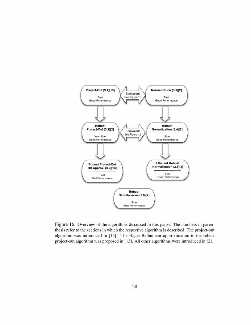
sion to the normalization algorithm and show in Section 3.5 how to implementthe robust normalization algorithm efficiently. For completeness in Section 3.6we describe the robust Gauss-Newton inverse compositional algorithm applied si-multaneously to the shape and appearance variation. While being considerablyslower this algorithm performs better than the other robust algorithms and shouldtherefore be considered for applications with less stringent real-time demands.See Figure 16 for an overview of the algorithms discussed in this paper.

In Section 4 we quantitativly evaluate all of the fitting algorithms on syn-thetic data. In particular we show that the efficient robust normalization algorithmoutperforms the Hager-Belhumeur algorithm [13]. We furthermore demonstratesuccessful face tracking using the robust normalization algorithm on a numberof image sequences containing occlusion. The overall tracking algorithm runs ataround 8 frames-per-second in Matlab and at around an estimated 50 frames-per-second in C.

2 Construction With OcclusionWe first define AAMs and then describe how they are constructed from train-

ing data with occlusion. The input consists of a collection of training images ofthe faces to be modeled with the location of all of the visible mesh vertices ineach of the images marked. Due to self-occlusion, e.g. when generating a modelacross large changes in pose, or due to occlusion by an object, only a subset of thevertices may be visible in any given training image. In the following we use thedefinition of an independent AAM which omits the combined PCA across shapeand appearance [15].

2.1 ShapeThe shape of an AAM is defined by a triangulated mesh and in particular thevertex locations of the mesh. Mathematically, we define the shape s of an AAMas the xy-coordinates of the v vertices that make up the mesh:

s = (x1, y1, x2, y2, . . . , xv, yv)T. (1)

AAMs allow linear shape variation; i.e., the shape s can be expressed as a baseshape s0 plus a linear combination of n shape vectors si:

s = s0 +n∑

i=1

pisi (2)

3

where the coefficients pi are the shape parameters. Since we can perform a linearre-parameterization, wherever necessary we assume that the shape vectors si areorthonormal.

2.1.1 Computing the Base Mesh s0 with Occlusion

In traditional AAMs [6,15] all of the mesh vertices s are marked in every trainingimage. The base mesh s0 is then constructed using the Procrustes algorithm [8]. Inthe presence of occlusion the situation is complicated by the fact that not all of themesh vertices are marked in every training image. The outline of the Procrustesalgorithm stays the same, however only vertices visible in a given training imageare used. The Procrustes algorithm with occlusion is then:

1. Initialize the base mesh s0 to be the visible vertices of the mesh s in any oneof the training images.

2. Repeat until the estimate of s0 converges:

(a) For each training image, align s to the current s0 with a 2D similaritytransform (rotation, translation, and scale) using the vertices commonto s and s0.

(b) Update s0 as the mean of all of the aligned meshes s.

In Step (2) only images are used where there is substantial overlap between theirvisible s and the current estimate of s0. In our implementation, substantial overlapmeans over 50% of the vertices in s are in s0. In Step (2b) only the vertices thatappear in at least one of the s are updated. The mean for each vertex is computedacross the images in which it is visible.

2.1.2 Computing the Shape Variation si with Occlusion

In traditional AAMs [6,15] the shape vectors si are computed by first aligning ev-ery training shape vector s with the base mesh s0 using a similarity transform [6].The mean shape (i.e., the base mesh s0) is subtracted from each shape vector. Prin-cipal Components Analysis [11] is then performed on the aligned shape vectorss. In the case of occlusion only the visible vertices are aligned to the base mesh.Principal Components Analysis with missing data [17, 18] is then performed onthe aligned shape vectors s. The shape vectors si are then set to be the orthonor-malized eigenvectors with the largest eigenvalues. As is common practice [6] we

4

retain enough shape modes to explain 95% of the observed variation in the trainingset.

2.2 AppearanceAs a convenient abuse of terminology, let s0 also denote the pixels x = (x, y)T

that lie inside the base mesh s0. The appearance of a AAM is then an image A(x)defined over the pixels x ∈ s0. AAMs allow linear appearance variation. Thismeans that the appearance A(x) can be expressed as a base appearance A0(x),plus a linear combination of m appearance images Ai(x):

A(x) = A0(x) +m∑

i=1

λiAi(x) ∀ x ∈ s0 (3)

where the coefficients λi are the appearance parameters. As in Section 2.1, wher-ever necessary we assume that the images Ai are orthonormal.

2.2.1 Computing the Appearance Variation Ai with Occlusion

In traditional AAMs the appearance vectors Ai are computed by warping all ofthe input images onto the base mesh using the piecewise affine warps defined be-tween the training shape vector s and the base mesh s0 [6]. Principal ComponentsAnalysis is then applied to the resulting images. In the case of occlusion the shapenormalized input images are incomplete. If any of the vertices of a triangle are notvisible in the training image, that triangle will be missing in the training image.Again, we use Principal Components Analysis with missing data [17,18] to com-pute the appearance vectors Ai. The appearance vectors Ai are then set to be theorthonormalized eigenvectors with the largest eigenvalues. As in the computationof the shape model, we retain enough appearance modes to explain 95% of theobserved variation in the training set.

2.3 ExperimentsIn order to evaluate AAMs constructed with occlusion we start with fully labeledimage sequences of five subjects in which randomly selected regions are artifi-cially occluded. Using artificially occluded data in this way allows for a moresystematic evaluation of how the algorithms perform with varying degrees of oc-clusion. In Section 2.3.4 we include experiments with natural occlusion. In total

5

(a) (b) (c)

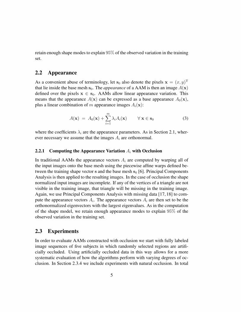
Figure 1: Artificially occluded data. (a) Original images with all mesh vertices s visible.(b) Images with 10% of the face region occluded. (c) Images with 50% of the face regionoccluded. Only non-occluded vertices are used in the AAM construction.

0.05 0.10 0.15 0.20 0.25 0.30 0.35 0.40 0.45 0.500

0.1

0.2

0.3

0.4

0.5

% Occlusion

Ave

rage

Dis

tanc

e [p

ixel

]

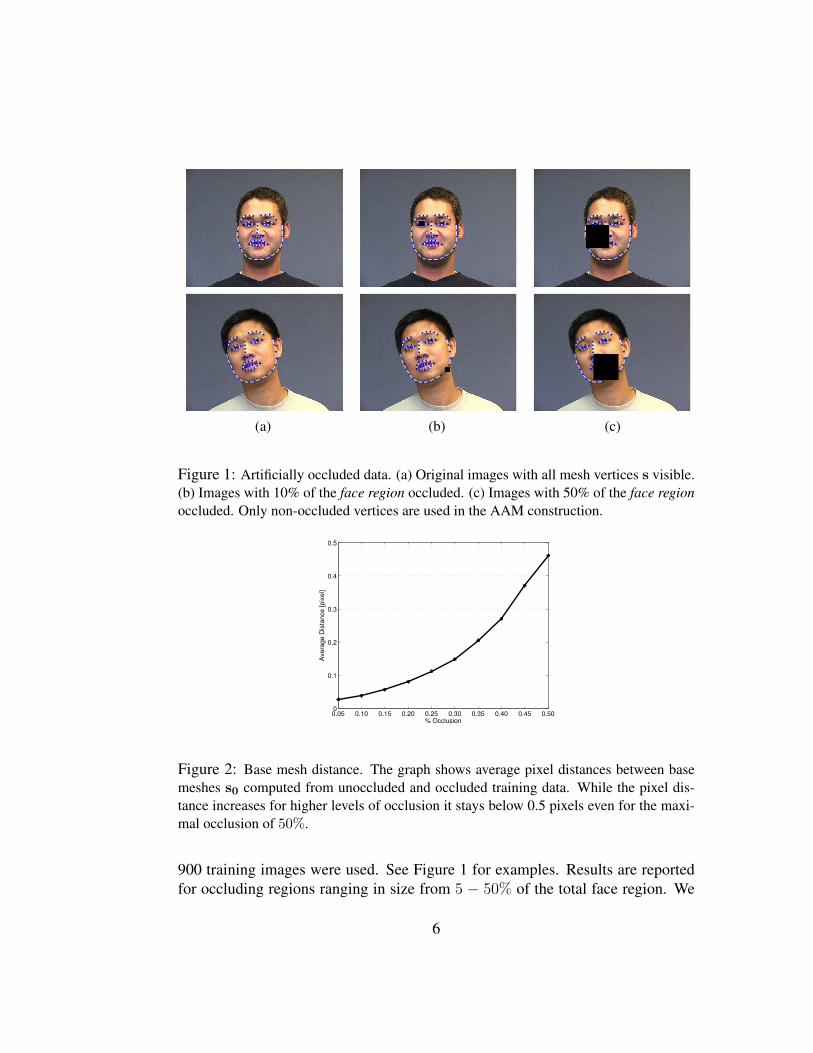
Figure 2: Base mesh distance. The graph shows average pixel distances between basemeshes s0 computed from unoccluded and occluded training data. While the pixel dis-tance increases for higher levels of occlusion it stays below 0.5 pixels even for the maxi-mal occlusion of 50%.

900 training images were used. See Figure 1 for examples. Results are reportedfor occluding regions ranging in size from 5 − 50% of the total face region. We

6

0.05 0.10 0.15 0.20 0.25 0.30 0.35 0.40 0.45 0.500.8

0.85

0.9

0.95

1

Percent occlusion

Sha

pe E

nerg

y O

verla

p [%

]

0.05 0.10 0.15 0.20 0.25 0.30 0.35 0.40 0.45 0.500.8

0.85

0.9

0.95

1

Percent occlusion

App

eara

nce

Ene

rgy

Ove

rlap

[%]

(a) Shape energy overlap SE (b) Appearance energy overlap AE

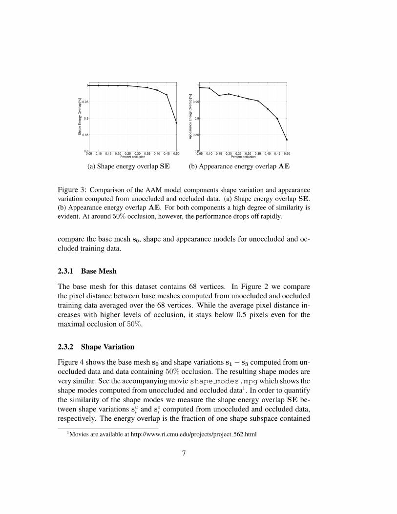
Figure 3: Comparison of the AAM model components shape variation and appearancevariation computed from unoccluded and occluded data. (a) Shape energy overlap SE.(b) Appearance energy overlap AE. For both components a high degree of similarity isevident. At around 50% occlusion, however, the performance drops off rapidly.

compare the base mesh s0, shape and appearance models for unoccluded and oc-cluded training data.

2.3.1 Base Mesh

The base mesh for this dataset contains 68 vertices. In Figure 2 we comparethe pixel distance between base meshes computed from unoccluded and occludedtraining data averaged over the 68 vertices. While the average pixel distance in-creases with higher levels of occlusion, it stays below 0.5 pixels even for themaximal occlusion of 50%.

2.3.2 Shape Variation

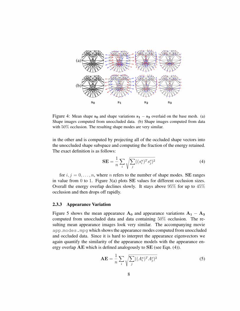
Figure 4 shows the base mesh s0 and shape variations s1− s3 computed from un-occluded data and data containing 50% occlusion. The resulting shape modes arevery similar. See the accompanying movie shape modes.mpgwhich shows theshape modes computed from unoccluded and occluded data1. In order to quantifythe similarity of the shape modes we measure the shape energy overlap SE be-tween shape variations su

i and soi computed from unoccluded and occluded data,

respectively. The energy overlap is the fraction of one shape subspace contained

1Movies are available at http://www.ri.cmu.edu/projects/project 562.html

7

(a)

(b)

s0 s1 s2 s3

Figure 4: Mean shape s0 and shape variations s1 − s3 overlaid on the base mesh. (a)Shape images computed from unoccluded data. (b) Shape images computed from datawith 50% occlusion. The resulting shape modes are very similar.

in the other and is computed by projecting all of the occluded shape vectors intothe unoccluded shape subspace and computing the fraction of the energy retained.The exact definition is as follows:

SE =1

n

∑i

√∑j

((sui )

T soj)

2 (4)

for i, j = 0, . . . , n, where n refers to the number of shape modes. SE rangesin value from 0 to 1. Figure 3(a) plots SE values for different occlusion sizes.Overall the energy overlap declines slowly. It stays above 95% for up to 45%occlusion and then drops off rapidly.

2.3.3 Appearance Variation

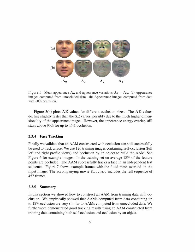
Figure 5 shows the mean appearance A0 and appearance variations A1 − A3

computed from unoccluded data and data containing 50% occlusion. The re-sulting mean appearance images look very similar. The accompanying movieapp modes.mpgwhich shows the appearance modes computed from unoccludedand occluded data. Since it is hard to interpret the appearance eigenvectors weagain quantify the similarity of the appearance models with the appearance en-ergy overlap AE which is defined analogously to SE (see Eqn. (4)).

AE =1

n

∑i

√∑j

((Aui )

T Aoj)

2 (5)

8

(a)

(b)

A0 A1 A2 A3

Figure 5: Mean appearance A0 and appearance variations A1 − A3. (a) Appearanceimages computed from unoccluded data. (b) Appearance images computed from datawith 50% occlusion.

Figure 3(b) plots AE values for different occlusion sizes. The AE valuesdecline slightly faster than the SE values, possibly due to the much higher dimen-sionality of the appearance images. However, the appearance energy overlap stillstays above 90% for up to 45% occlusion.

2.3.4 Face Tracking

Finally we validate that an AAM constructed with occlusion can still successfullybe used to track a face. We use 120 training images containing self-occlusion (fullleft and right profile views) and occlusion by an object to build the AAM. SeeFigure 6 for example images. In the training set on average 18% of the featurepoints are occluded. The AAM successfully tracks a face in an independent testsequence. Figure 7 shows example frames with the fitted mesh overlaid on theinput image. The accompanying movie fit.mpg includes the full sequence of457 frames.

2.3.5 Summary

In this section we showed how to construct an AAM from training data with oc-clusion. We empirically showed that AAMs computed from data containing upto 45% occlusion are very similar to AAMs computed from unoccluded data. Wefurthermore demonstrated good tracking results using an AAM constructed fromtraining data containing both self-occlusion and occlusion by an object.

9

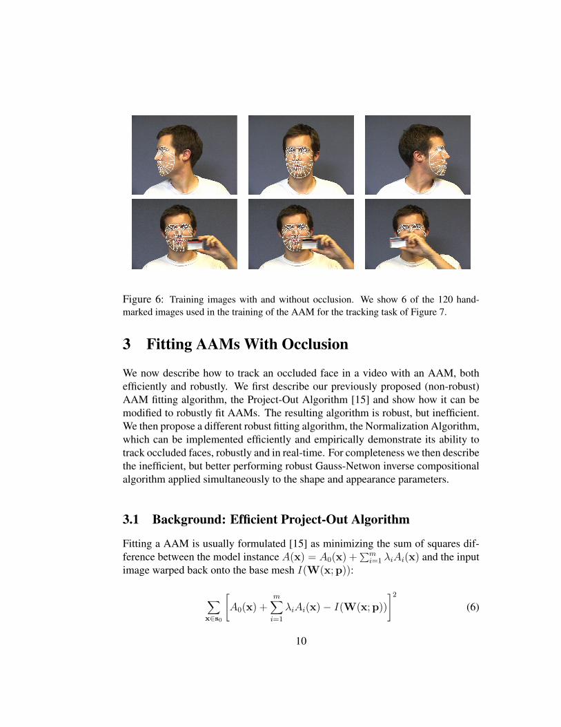
Figure 6: Training images with and without occlusion. We show 6 of the 120 hand-marked images used in the training of the AAM for the tracking task of Figure 7.

3 Fitting AAMs With Occlusion

We now describe how to track an occluded face in a video with an AAM, bothefficiently and robustly. We first describe our previously proposed (non-robust)AAM fitting algorithm, the Project-Out Algorithm [15] and show how it can bemodified to robustly fit AAMs. The resulting algorithm is robust, but inefficient.We then propose a different robust fitting algorithm, the Normalization Algorithm,which can be implemented efficiently and empirically demonstrate its ability totrack occluded faces, robustly and in real-time. For completeness we then describethe inefficient, but better performing robust Gauss-Netwon inverse compositionalalgorithm applied simultaneously to the shape and appearance parameters.

3.1 Background: Efficient Project-Out Algorithm

Fitting a AAM is usually formulated [15] as minimizing the sum of squares dif-ference between the model instance A(x) = A0(x) +

∑mi=1 λiAi(x) and the input

image warped back onto the base mesh I(W(x;p)):

∑x∈s0

[A0(x) +

m∑i=1

λiAi(x)− I(W(x;p))

]2

(6)

10

Figure 7: Example frames of a test sequence showing accurate tracking with an AAMconstructed with occlusion. See the accompanying movie fit.mpg for the full sequenceof 457 frames.

where the sum is performed over all of the pixels x in the base mesh s0. In thisequation, the warp W is the piecewise affine warp from the base mesh s0 to thecurrent AAM shape s defined by the vertices. Hence, W is a function of theshape parameters p. For ease of notation, in this paper we have omitted mentionof the 2D similarity transformation that is used to normalize the shape of an AAM.In [15] we showed how to include this warp into W. The goal of AAM fitting isto minimize the expression in Equation (6) simultaneously with respect to theshape p and appearance λ parameters. The “project-out” inverse compositionalalgorithm [3] and its extension to 2D AAMs was proposed in [15]. See Figure 8for a summary. The algorithm performs the non-linear optimization of Equation6 in two steps (similar to Hager and Belhumeur [13]). The shape parameters pare found through non-linear optimization in a subspace in which the appearancevariation can be ignored. This is achieved by “projecting out” the appearance

11

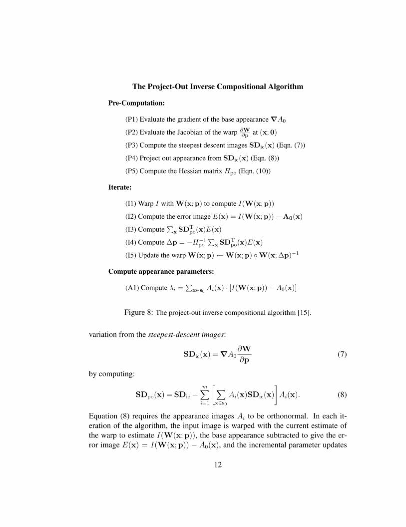
The Project-Out Inverse Compositional Algorithm

Pre-Computation:

(P1) Evaluate the gradient of the base appearance ∇A0

(P2) Evaluate the Jacobian of the warp ∂W∂p at (x;0)

(P3) Compute the steepest descent images SDic(x) (Eqn. (7))

(P4) Project out appearance from SDic(x) (Eqn. (8))

(P5) Compute the Hessian matrix Hpo (Eqn. (10))

Iterate:

(I1) Warp I with W(x;p) to compute I(W(x;p))

(I2) Compute the error image E(x) = I(W(x;p))−A0(x)

(I3) Compute∑

x SDTpo(x)E(x)

(I4) Compute ∆p = −H−1po

∑x SDT

po(x)E(x)

(I5) Update the warp W(x;p)←W(x;p) ◦W(x;∆p)−1

Compute appearance parameters:

(A1) Compute λi =∑

x∈s0 Ai(x) · [I(W(x;p))−A0(x)]

Figure 8: The project-out inverse compositional algorithm [15].

variation from the steepest-descent images:

SDic(x) = ∇A0∂W

∂p(7)

by computing:

SDpo(x) = SDic −m∑

i=1

[∑x∈s0

Ai(x)SDic(x)

]Ai(x). (8)

Equation (8) requires the appearance images Ai to be orthonormal. In each it-eration of the algorithm, the input image is warped with the current estimate ofthe warp to estimate I(W(x;p)), the base appearance subtracted to give the er-ror image E(x) = I(W(x;p)) − A0(x), and the incremental parameter updates

12

computed:

∆p = −H−1po

∑x∈s0

SDpo(x)[I(W(x;p))− A0(x)] (9)

using the Project-Out Hessian:

Hpo =∑x∈s0

SDpo(x)TSDpo(x). (10)

The incremental warp W(x; ∆p) is then inverted and composed with the currentestimate to give the new estimate W(x;p)◦W(x; ∆p)−1. In the second step, theappearance parameters λ can then be computed as:

λi =∑x∈s0

Ai(x) · [I(W(x;p))− A0(x)] . (11)

If there are n shape parameters, m appearance parameters, and N pixels in thebase appearance A0, the pre-computation takes time O(n2 · N + m · N) wherethe slowest step is the computation of the Hessian in Step P5 which alone takestime O(n2 · N). The online cost per iteration is just O(n · N + n3) and thepost-computation cost is O(m · N). In all cases we iterate the algorithm untilconvergence or for a sufficient (fixed) number of times. A implementation of thisalgorithm in “C” runs at 230 frames per second on a dual 3GHz Pentium 4 Xeonfor typical values of n, m and N [15].

3.2 Robust Fitting: Inefficient Algorithm

Occluded pixels in the input image can be viewed as “outliers”. In order to dealwith outliers in a least-squares optimization framework a robust error function canbe used [4, 13, 14]. The goal of robustly fitting a AAM is then to minimize

∑x∈s0

%

[A0(x) +m∑

i=1

λiAi(x)− I(W(x;p))

]2

; σ

(12)

with respect to the shape p and appearance λ parameters where %(t; σ) is a sym-metric robust error function [14] and σ is a vector of scale parameters. For easeof explanation we treat the scale parameters as known constants and drop them inthe following. In comparison to the project-out algorithm the expressions for the

13

incremental parameter update ∆p (Equation 9) and the Hessian Hpo (Equation 10)have to be weighted by the error function %′(Eapp(x)2), where:

Eapp(x) = I(W(x;p))−[A0(x) +

m∑i=1

λiAi(x)

](13)

Equation (9) then becomes:

∆p = −H−1ρ

∑x∈s0

%′(Eapp(x)2)SDpo(x)Eapp(x) (14)

with:Hρ =

∑x∈s0

%′(Eapp(x)2)SDpo(x)TSDpo(x). (15)

The steepest descent images SDpo also have to be re-computed using Equation (8)because the appearance images are no longer orthonormal. The appearance im-ages Ai must be re-orthonormalized with respect to the new inner product:

∑x

%′(Eapp(x)2

)Ai(x) Aj(x) =

{1 if i = j0 if i 6= j

(16)

Steps (P3)-(P5) in Figure 8 can therefore no longer be pre-computed and have tobe moved inside the iteration. As a result the robust project-out inverse compo-sitional algorithm is very inefficient. See [2] for more details. An approxima-tion is to ignore the lack of orthogonality and just continue to use the Euclideanproject out steepest descent images. This approach is taken in [13], where theH-Algorithm [9] is used to keep the Hessian constant to yield an efficient algo-rithm. As we will show in Section 4 this approximation while fast, leads to poorperformance.

3.3 Project-out vs. NormalizationWe now describe a slightly different algorithm to minimize the expression inEquation (6), the normalization inverse compositional algorithm [2]. As we willshow, the robust extension of the normalization algorithm can be implementedvery efficiently. An alternative way of dealing with the linear appearance varia-tion in Equation (6) is to project out the appearance images Ai from the singleerror image Eapp rather than the large number of steepest descent images SDic.This normalization can be achieved by normalizing the error image so that the

14

component of the error image in the direction Ai is zero. In particular, the nor-malization step consists of:

λi =∑x

Ai(x) E(x) for i = 1, . . . ,m

Eapp(x) ← E(x)−m∑

i=1

λi Ai(x).(17)

As indicated, in the process of normalizing Eapp in this way the appearance pa-rameters λi are estimated. In comparison to the project-out algorithm in Figure 8steps (P4) and (A1) are removed and the normalization step of Equation (17) isadded after the computation of the error image E(x) in step (I2). The equivalenceof the project-out and normalization algorithms is shown empirically in Section 4.

3.4 Robust Normalization AlgorithmThe goal of the normalization step in Equation (17) is to make the component ofthe error image in the direction Ai to be zero, whilst computing λi at the sametime. We now reformulate this step using the robust error function. We wishto compute updates to the appearance parameters ∆λ = (∆λ1, . . . , ∆λm)T thatminimize: ∑

x

%′(Eapp(x)2

) [Eapp(x)−

m∑i=1

∆λiAi(x)

]2

. (18)

The least squares minimum of this expression is:

∆λ = H−1A

∑x

%′(Eapp(x)2

)AT(x)Eapp(x) (19)

where A(x) = (A1(x), . . . , Am(x)) and HA is the appearance Hessian:

HA =∑x

%′(Eapp(x)2

)A(x)TA(x). (20)

The steepest descent parameter updates and the Hessian are computed as in Equa-tions (14) and (15). Note that we avoid re-orthonormalization of the appearanceimages Ai in every iteration as is required in the robust algorithm of Section 3.2.

3.5 Efficient Robust FittingDue to the computation of the appearance Hessian HA and the Hessian Hρ inevery iteration the robust normalization algorithm is also inefficient. However,

15

most of this computation can be moved outside of the iteration if we assume thatthe outliers are spatially coherent. To make use of this assumption we subdividethe base appearance A0 into triangles according to the triangulation of the basemesh s0. Suppose there are K triangles T1, T2, . . . , TK with Ni pixels in the ith

triangle. Equation (15) can then be rewritten:

Hρ =K∑

i=1

∑x∈Ti

%′(Eapp(x)2

)SDT

ic(x)SDic(x). (21)

Based on the spatial coherence of the outliers [1], assume that %′(Eapp(x)2) isconstant in each triangle; i.e. assume %′(Eapp(x)2) = %′i, say, for all x ∈ Ti. Inpractice this assumption only holds approximately and so %′i must be estimatedfrom %′(Eapp(x)2), for example by setting it to be the mean value computed overthe triangle [1]. Equation (21) can then be rearranged to:

Hρ =K∑

i=1

%′i∑x∈Ti

SDTic(x)SDic(x). (22)

The internal part of this expression does not depend on the robust function %′ andso is constant across iterations. Denote:

H iρ =

∑x∈Ti

SDTic(x)SDic(x). (23)

The Hessian H iρ is the Hessian for the triangle Ti and can be precomputed. Equa-

tion (22) then simplifies to:

Hρ =K∑

i=1

%′i ·H iρ. (24)

Although this Hessian does vary from iteration to iteration, the cost of computingit is minimal. The same spatial coherence approximation can be made for theappearance Hessian of Equation (20). The efficient robust normalization inversecompositional algorithm is summarized in Figure 9.

3.6 Robust Simultaneous Fitting AlgorithmIn this paper we have described a variety of efficient gradient descent algorithms.All of these algorithms are approximations to the simultaneous Gauss-Newton

16

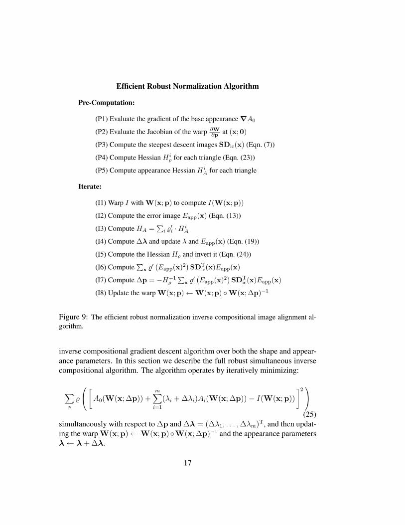
Efficient Robust Normalization Algorithm

Pre-Computation:

(P1) Evaluate the gradient of the base appearance ∇A0

(P2) Evaluate the Jacobian of the warp ∂W∂p at (x;0)

(P3) Compute the steepest descent images SDic(x) (Eqn. (7))

(P4) Compute Hessian H iρ for each triangle (Eqn. (23))

(P5) Compute appearance Hessian H iA for each triangle

Iterate:

(I1) Warp I with W(x;p) to compute I(W(x;p))

(I2) Compute the error image Eapp(x) (Eqn. (13))

(I3) Compute HA =∑

i %′i ·H i

A

(I4) Compute ∆λ and update λ and Eapp(x) (Eqn. (19))

(I5) Compute the Hessian Hρ and invert it (Eqn. (24))

(I6) Compute∑

x %′(Eapp(x)2

)SDT

ic(x)Eapp(x)

(I7) Compute ∆p = −H−1%

∑x %′

(Eapp(x)2

)SDT

ic(x)Eapp(x)

(I8) Update the warp W(x;p)←W(x;p) ◦W(x;∆p)−1

Figure 9: The efficient robust normalization inverse compositional image alignment al-gorithm.

inverse compositional gradient descent algorithm over both the shape and appear-ance parameters. In this section we describe the full robust simultaneous inversecompositional algorithm. The algorithm operates by iteratively minimizing:

∑x

%

[A0(W(x; ∆p)) +m∑

i=1

(λi + ∆λi)Ai(W(x; ∆p))− I(W(x;p))

]2(25)

simultaneously with respect to ∆p and ∆λ = (∆λ1, . . . , ∆λm)T, and then updat-ing the warp W(x;p)←W(x;p)◦W(x; ∆p)−1 and the appearance parametersλ← λ + ∆λ.

17

To simplify the notation, denote:

q =

(pλ

)and similarly ∆q =

(∆p∆λ

); (26)

i.e. q is an n + m dimensional column vector containing the warp parameters pconcatenated with the appearance parameters λ. Denote the n + m dimensionalsteepest-descent images as follows:

SDsim(x) =(

∇A∂W∂p1

, . . . ,∇A∂W∂pn

, A1(x), . . . , Am(x))

(27)

where ∇A is defined as

∇A = ∇A0 +m∑

i=1

λi∇Ai. (28)

We can then compute the parameter update ∆q as

∆q = −H−1sim,%

∑x

%′(Eapp(x)2

)SDT

sim(x)Eapp(x) (29)

where:Hsim,% =

∑x

%′(Eapp(x)2

)SDT

sim(x)SDsim(x) (30)

and Eapp is defined as in Equation (13). See [2] for more details. Since thesteepest descent images SDsim depend on the appearance parameters λ throughEquation (28) they have to be re-computed in every iteration. The algorithm istherefore inefficient. The robust simultaneous algorithm is summarized in Fig-ure 10.

4 EvaluationWe evaluate all of the fitting algorithms described in Section 3 on synthetic data.We then demonstrate successful face tracking using the robust normalization al-gorithm on a number of image sequences containing occlusion.

4.1 Quantitative ComparisonWe first compare the performance of the various non-robust and robust fittingalgorithms described earlier on synthetic data. In these experiments, we restrict

18

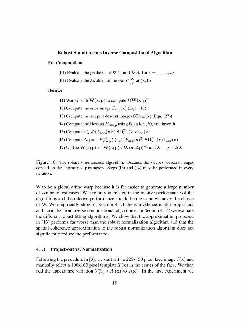
Robust Simultaneous Inverse Compositional Algorithm

Pre-Computation:

(P1) Evaluate the gradients of ∇A0 and ∇Ai for i = 1, . . . ,m

(P2) Evaluate the Jacobian of the warp ∂W∂p at (x;0)

Iterate:

(I1) Warp I with W(x;p) to compute I(W(x;p))

(I2) Compute the error image Eapp(x) (Eqn. (13))

(I3) Compute the steepest descent images SDsim(x) (Eqn. (27))

(I4) Compute the Hessian Hsim,% using Equation (30) and invert it

(I5) Compute∑

x %′(Eapp(x)2

)SDT

sim(x)Eapp(x)

(I6) Compute ∆q = −H−1sim,%

∑x %′

(Eapp(x)2

)SDT

sim(x)Eapp(x)

(I7) Update W(x;p)←W(x;p) ◦W(x;∆p)−1 and λ← λ + ∆λ

Figure 10: The robust simultaneous algorithm. Because the steepest descent imagesdepend on the appearance parameters, Steps (I3) and (I4) must be performed in everyiteration.

W to be a global affine warp because it is far easier to generate a large numberof synthetic test cases. We are only interested in the relative performance of thealgorithms and the relative performance should be the same whatever the choiceof W. We empirically show in Section 4.1.1 the equivalence of the project-outand normalization inverse compositional algorithms. In Section 4.1.2 we evaluatethe different robust fitting algorithms. We show that the approximation proposedin [13] performs far worse than the robust normalization algorithm and that thespatial coherence approximation to the robust normalization algorithm does notsignificantly reduce the performance.

4.1.1 Project-out vs. Normalization

Following the procedure in [3], we start with a 225x150 pixel face image I(x) andmanually select a 100x100 pixel template T (x) in the center of the face. We thenadd the appearance variation

∑mi=1 λiAi(x) to I(x). In the first experiment we

19

1 2 3 4 5 6 7 8 9 100

10

20

30

40

50

60

70

80

90

100

Point Sigma

% C

onve

rged

PON

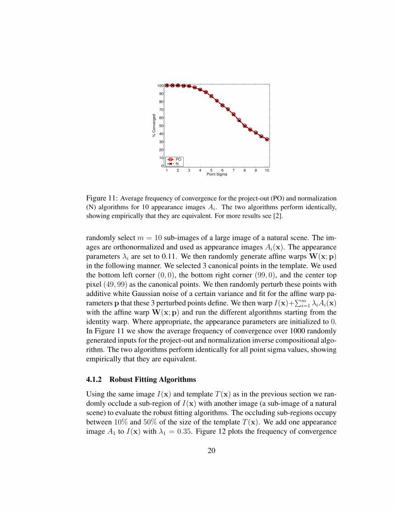
Figure 11: Average frequency of convergence for the project-out (PO) and normalization(N) algorithms for 10 appearance images Ai. The two algorithms perform identically,showing empirically that they are equivalent. For more results see [2].

randomly select m = 10 sub-images of a large image of a natural scene. The im-ages are orthonormalized and used as appearance images Ai(x). The appearanceparameters λi are set to 0.11. We then randomly generate affine warps W(x;p)in the following manner. We selected 3 canonical points in the template. We usedthe bottom left corner (0, 0), the bottom right corner (99, 0), and the center toppixel (49, 99) as the canonical points. We then randomly perturb these points withadditive white Gaussian noise of a certain variance and fit for the affine warp pa-rameters p that these 3 perturbed points define. We then warp I(x)+

∑mi=1 λiAi(x)

with the affine warp W(x;p) and run the different algorithms starting from theidentity warp. Where appropriate, the appearance parameters are initialized to 0.In Figure 11 we show the average frequency of convergence over 1000 randomlygenerated inputs for the project-out and normalization inverse compositional algo-rithm. The two algorithms perform identically for all point sigma values, showingempirically that they are equivalent.

4.1.2 Robust Fitting Algorithms

Using the same image I(x) and template T (x) as in the previous section we ran-domly occlude a sub-region of I(x) with another image (a sub-image of a naturalscene) to evaluate the robust fitting algorithms. The occluding sub-regions occupybetween 10% and 50% of the size of the template T (x). We add one appearanceimage A1 to I(x) with λ1 = 0.35. Figure 12 plots the frequency of convergence

20

1 2 3 4 5 6 7 8 9 100

10

20

30

40

50

60

70

80

90

100

Point Sigma

% C

onve

rged

10% Occlusion

RSICRPORPO−HBRNERN

1 2 3 4 5 6 7 8 9 100

10

20

30

40

50

60

70

80

90

100

Point Sigma

% C

onve

rged

25% Occlusion

RSICRPORPO−HBRNERN

1 2 3 4 5 6 7 8 9 100

10

20

30

40

50

60

70

80

90

100

Point Sigma

% C

onve

rged

40% Occlusion

RSICRPORPO−HBRNERN

1 2 3 4 5 6 7 8 9 100

10

20

30

40

50

60

70

80

90

100

Point Sigma

% C

onve

rged

50% Occlusion

RSICRPORPO−HBRNERN

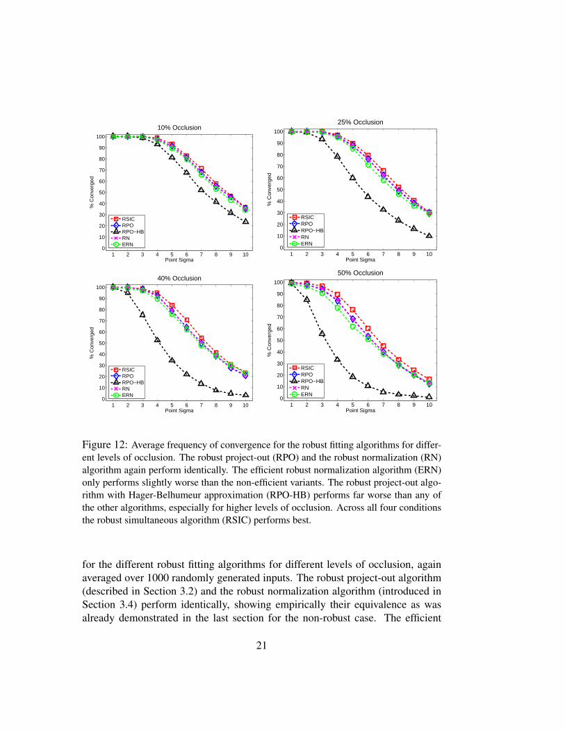
Figure 12: Average frequency of convergence for the robust fitting algorithms for differ-ent levels of occlusion. The robust project-out (RPO) and the robust normalization (RN)algorithm again perform identically. The efficient robust normalization algorithm (ERN)only performs slightly worse than the non-efficient variants. The robust project-out algo-rithm with Hager-Belhumeur approximation (RPO-HB) performs far worse than any ofthe other algorithms, especially for higher levels of occlusion. Across all four conditionsthe robust simultaneous algorithm (RSIC) performs best.

for the different robust fitting algorithms for different levels of occlusion, againaveraged over 1000 randomly generated inputs. The robust project-out algorithm(described in Section 3.2) and the robust normalization algorithm (introduced inSection 3.4) perform identically, showing empirically their equivalence as wasalready demonstrated in the last section for the non-robust case. The efficient

21

robust normalization algorithm (described in Section 3.5) trails the robust nor-malization algorithm only slightly in performance, therefore justifying its use. Fi-nally the robust project-out algorithm with Hager-Belhumeur approximation (nore-orthonormalization of the appearance images and use of the H-Algorithm [9]to keep the Hessian constant) performs far worse than the other algorithms, espe-cially for higher levels of occlusion. Across all conditions, the robust simultane-ous algorithm performs best.

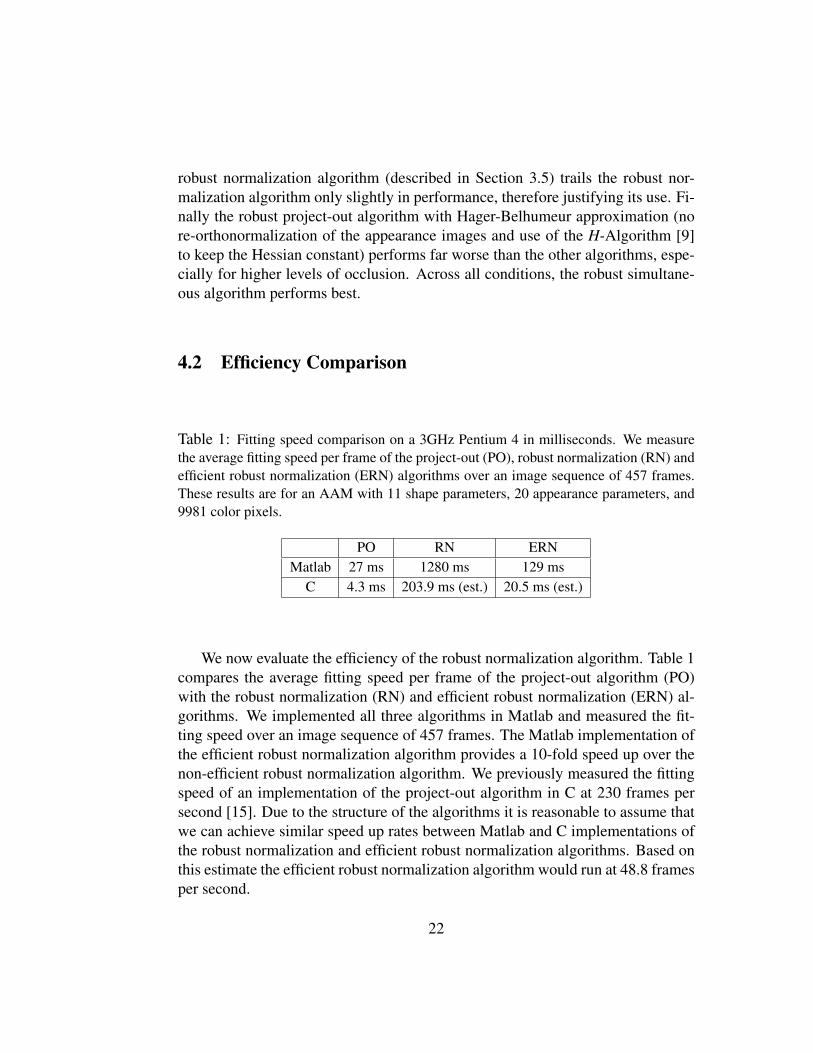
4.2 Efficiency Comparison

Table 1: Fitting speed comparison on a 3GHz Pentium 4 in milliseconds. We measurethe average fitting speed per frame of the project-out (PO), robust normalization (RN) andefficient robust normalization (ERN) algorithms over an image sequence of 457 frames.These results are for an AAM with 11 shape parameters, 20 appearance parameters, and9981 color pixels.

PO RN ERNMatlab 27 ms 1280 ms 129 ms

C 4.3 ms 203.9 ms (est.) 20.5 ms (est.)

We now evaluate the efficiency of the robust normalization algorithm. Table 1compares the average fitting speed per frame of the project-out algorithm (PO)with the robust normalization (RN) and efficient robust normalization (ERN) al-gorithms. We implemented all three algorithms in Matlab and measured the fit-ting speed over an image sequence of 457 frames. The Matlab implementation ofthe efficient robust normalization algorithm provides a 10-fold speed up over thenon-efficient robust normalization algorithm. We previously measured the fittingspeed of an implementation of the project-out algorithm in C at 230 frames persecond [15]. Due to the structure of the algorithms it is reasonable to assume thatwe can achieve similar speed up rates between Matlab and C implementations ofthe robust normalization and efficient robust normalization algorithms. Based onthis estimate the efficient robust normalization algorithm would run at 48.8 framesper second.

22

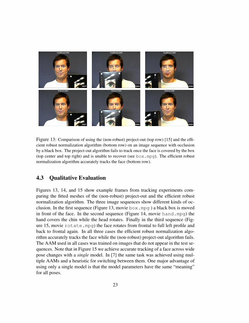
Figure 13: Comparison of using the (non-robust) project-out (top row) [15] and the effi-cient robust normalization algorithm (bottom row) on an image sequence with occlusionby a black box. The project-out algorithm fails to track once the face is covered by the box(top center and top right) and is unable to recover (see box.mpg). The efficient robustnormalization algorithm accurately tracks the face (bottom row).

4.3 Qualitative Evaluation

Figures 13, 14, and 15 show example frames from tracking experiments com-paring the fitted meshes of the (non-robust) project-out and the efficient robustnormalization algorithm. The three image sequences show different kinds of oc-clusion. In the first sequence (Figure 13, movie box.mpg ) a black box is movedin front of the face. In the second sequence (Figure 14, movie hand.mpg) thehand covers the chin while the head rotates. Finally in the third sequence (Fig-ure 15, movie rotate.mpg) the face rotates from frontal to full left profile andback to frontal again. In all three cases the efficient robust normalization algo-rithm accurately tracks the face while the (non-robust) project-out algorithm fails.The AAM used in all cases was trained on images that do not appear in the test se-quences. Note that in Figure 15 we achieve accurate tracking of a face across widepose changes with a single model. In [7] the same task was achieved using mul-tiple AAMs and a heuristic for switching between them. One major advantage ofusing only a single model is that the model parameters have the same “meaning”for all poses.

23

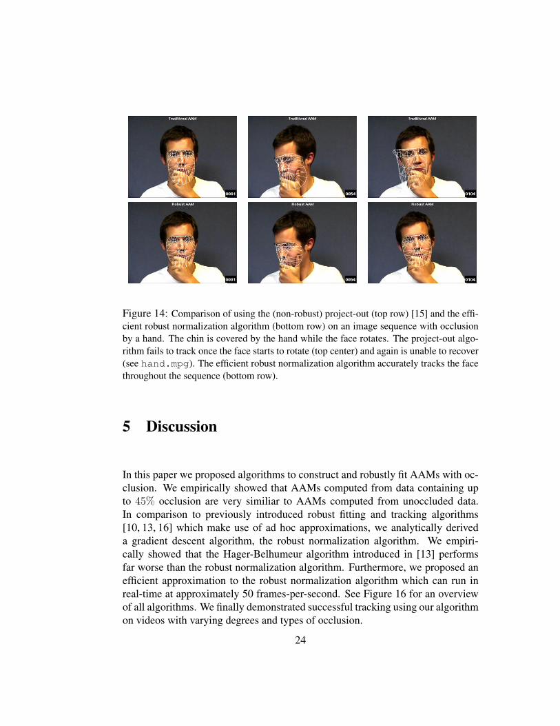
Figure 14: Comparison of using the (non-robust) project-out (top row) [15] and the effi-cient robust normalization algorithm (bottom row) on an image sequence with occlusionby a hand. The chin is covered by the hand while the face rotates. The project-out algo-rithm fails to track once the face starts to rotate (top center) and again is unable to recover(see hand.mpg). The efficient robust normalization algorithm accurately tracks the facethroughout the sequence (bottom row).

5 Discussion

In this paper we proposed algorithms to construct and robustly fit AAMs with oc-clusion. We empirically showed that AAMs computed from data containing upto 45% occlusion are very similiar to AAMs computed from unoccluded data.In comparison to previously introduced robust fitting and tracking algorithms[10, 13, 16] which make use of ad hoc approximations, we analytically deriveda gradient descent algorithm, the robust normalization algorithm. We empiri-cally showed that the Hager-Belhumeur algorithm introduced in [13] performsfar worse than the robust normalization algorithm. Furthermore, we proposed anefficient approximation to the robust normalization algorithm which can run inreal-time at approximately 50 frames-per-second. See Figure 16 for an overviewof all algorithms. We finally demonstrated successful tracking using our algorithmon videos with varying degrees and types of occlusion.

24

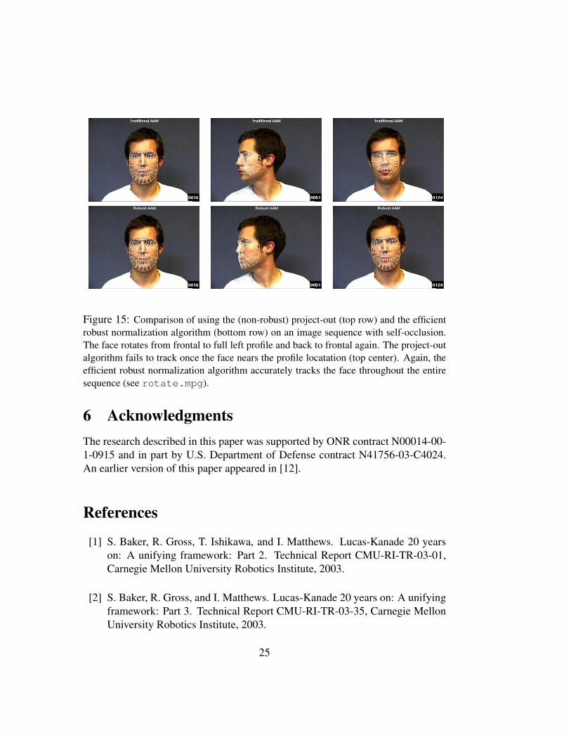
Figure 15: Comparison of using the (non-robust) project-out (top row) and the efficientrobust normalization algorithm (bottom row) on an image sequence with self-occlusion.The face rotates from frontal to full left profile and back to frontal again. The project-outalgorithm fails to track once the face nears the profile locatation (top center). Again, theefficient robust normalization algorithm accurately tracks the face throughout the entiresequence (see rotate.mpg).

6 AcknowledgmentsThe research described in this paper was supported by ONR contract N00014-00-1-0915 and in part by U.S. Department of Defense contract N41756-03-C4024.An earlier version of this paper appeared in [12].

References

[1] S. Baker, R. Gross, T. Ishikawa, and I. Matthews. Lucas-Kanade 20 yearson: A unifying framework: Part 2. Technical Report CMU-RI-TR-03-01,Carnegie Mellon University Robotics Institute, 2003.

[2] S. Baker, R. Gross, and I. Matthews. Lucas-Kanade 20 years on: A unifyingframework: Part 3. Technical Report CMU-RI-TR-03-35, Carnegie MellonUniversity Robotics Institute, 2003.

25

[3] S. Baker and I. Matthews. Lucas-Kanade 20 years on: A unifying frame-work. International Journal of Computer Vision, 56(3):221–255, February2004.

[4] M. Black and A. Jepson. Eigen-tracking: Robust matching and tracking ofarticulated objects using a view-based representation. International Journalof Computer Vision, 36(2):101–130, 1998.

[5] V. Blanz and T. Vetter. A morphable model for the synthesis of 3D faces. InComputer Graphics, Annual Conference Series (SIGGRAPH), pages 187–194, 1999.

[6] T. Cootes, G. Edwards, and C. Taylor. Active appearance models. IEEETransactions on Pattern Analysis and Machine Intelligence, 23(6):681–685,2001.

[7] T. Cootes, G. Wheeler, K. Walker, and C. Taylor. View-based active appear-ance models. Image and Vision Computing, 20:657–664, 2002.

[8] I.L. Dryden and K.V. Mardia. Statistical Shape Analysis. Wiley & Sons,1998.

[9] R. Dutter and P.J. Huber. Numerical methods for the nonlinear robust regres-sion problem. Journal of Statistical and Computational Simulation, 13:79–113, 1981.

[10] G.J. Edwards, T.J. Cootes, and C.J. Taylor. Advances in active appearancemodels. In International Conference on Computer Vision, pages 137–142,1999.

[11] K. Fukunaga. Introduction to statistical pattern recognition. AcademicPress, 1990.

[12] R. Gross, I. Matthews, and S. Baker. Constructing and fitting active appear-ance models with occlusion. In First IEEE Workshop on Face Processing inVideo (FPiV), 2004.

[13] G. Hager and P. Belhumeur. Efficient region tracking with parametric modelsof geometry and illumination. IEEE Transactions on Pattern Analysis andMachine Intelligence, 20(10):1025–1039, 1998.

26

[14] P.J. Huber. Robust Statistics. Wiley & Sons, 1981.

[15] I. Matthews and S. Baker. Active Appearance Models revisited. Interna-tional Journal of Computer Vision, 60(2):135–164, 2004.

[16] S. Sclaroff and J. Isidoro. Active blobs. In Proceedings of the IEEE Inter-national Conference on Computer Vision, pages 1146–1153, 1998.

[17] H. Shum, K. Ikeuchi, and R. Reddy. Principal component analysis withmissing data and its application to polyhedral object modeling. IEEE Trans-actions on Pattern Analysis and Machine Intelligence, 17(9):855–867, 1995.

[18] F. de la Torre and M. Black. A framework for robust subspace learning.International Journal of Computer Vision, 54(1):117–142, 2003.

27

Project-Out (3.1)[15]---------------------------

FastGood Performance

EquivalentSee Figure 11

RobustProject-Out (3.2)[2]---------------------------

Very SlowGood Performance

RobustNormalization (3.4)[2]

---------------------------Slow

Good Performance

Robust Project-OutHB Approx. (3.2)[13]---------------------------

FastBad Performance

Efficient RobustNormalization (3.5)[2]

---------------------------Fast

Good Performance

RobustSimultaneous (3.6)[2]

---------------------------Slow

Best Performance

Normalization (3.3)[2]---------------------------

FastGood Performance

EquivalentSee Figure 12

Figure 16: Overview of the algorithms discussed in this paper. The numbers in paren-thesis refer to the sections in which the respective algorithm is described. The project-outalgorithm was introduced in [15]. The Hager-Belhumeur approximation to the robustproject-out algorithm was proposed in [13]. All other algorithms were introduced in [2].

28