active contour methods on arbitrary graphs based on

Chapter 4

Active contour methods onarbitrary graphs based onpartial differential equations

Christos Sakaridisa, Nikos Kolotourosb, Kimon Drakopoulosc

and Petros Maragosd,*aDepartment of Information Technology and Electrical Engineering, ETH Z€urich, Zurich,

SwitzerlandbDepartment of Computer and Information Science, University of Pennsylvania,

Philadelphia, PA, United StatescMarshall School of Business, University of Southern California, Los Angeles, CA, United StatesdSchool of Electrical and Computer Engineering, National Technical University of Athens,

Athens, Greece*Corresponding author: e-mail: [email protected]

Chapter Outline1 Introduction 150

2 Background and related work 151

3 Active contours on graphs via

geometric approximations of

gradient and curvature 155

3.1 Geometric gradient

approximation on graphs 155

3.2 Geometric curvature

approximation on graphs 163

3.3 Gaussian smoothing on

graphs 166

4 Active contours on graphs

using a finite element

framework 169

4.1 Problem formulation

and numerical

approximation 169

4.2 Locally constrained contour

evolution 174

5 Experimental results 178

6 Conclusion 186

References 187

AbstractThis chapter formulates and compares two approaches that have been developed to

discretize over arbitrary graphs the partial differential equations (PDEs) of classical

active contour models with level sets, which have been widely used in image analysis

and computer vision. The first approach takes a finite difference path and proposes

geometric approximations of the fundamental continuous differential operators that

are involved in active contour PDEs, namely gradient and curvature, on graphs with

Handbook of Numerical Analysis, Vol. 20. https://doi.org/10.1016/bs.hna.2019.07.002

© 2019 Elsevier B.V. All rights reserved. 149

Cite as: C. Sakaridis, N. Kolotouros, K. Drakopoulos and P. Maragos, "Active contour methods on arbitrary graphs based on partial differential equations", in Handbook of Numerical Analysis, Vol.20: Processing, Analyzing and Learning of Images, Shapes, and Forms: Part 2, R. Kimmel and X.-C. Tai, Eds., Elsevier North-Holland, 2019, pp.149-190. https://doi.org/10.1016/bs.hna.2019.07.002

https://doi.org/10.1016/bs.hna.2019.07.002

arbitrary vertex and edge configuration. The second approach leverages finite elements

to approximate the solution of these PDEs on graphs with arbitrary vertex configuration

that constitute a triangulation. We present numerical algorithms and compare both

approaches while using them to successfully apply the popular models of geodesic

active contours (GACs) and active contours without edges (ACWE) to arbitrary 2D

graphs for graph cluster detection and image segmentation.

Keywords: Active contours on graphs, Graph segmentation, Discretized partial differ-

ential equations

AMS Classification Codes: 35Q68, 35R02, 60D05, 65D25, 65M60, 68U10

1 Introduction

Evolution of curves via active contour models has been applied extensively in

computer vision for image segmentation. In the standard image setting which

involves a regular grid of pixels, the discretization of partial differential equa-

tions (PDEs) governing the motion of active contours is well-established

(Osher and Sethian, 1988) and ensures proper convergence of the contour to

object boundaries. Recently, active contour models based on level set PDE for-

mulations have been extended (Drakopoulos and Maragos, 2012; Kolotouros

and Maragos, 2017; Sakaridis et al., 2017) to handle more general inputs in

the form of graphs whose vertices are arbitrarily distributed in a two-dimensional

Euclidean space. In particular, the input in this case consists of:

1. an undirected graph G¼ ðV,EÞ, where V ¼ vi 22 : i¼ 1,…,n� �

and

E �V�V, and2. a real-valued function I :V! defined on the vertices of the graph,

which resembles the image function in the standard grid setting. For the

rest of the paper, we will use the term image function to refer to I.

Applications of segmentation of such graphs span not only image processing

but also geographical information systems and generally any field where data

can assume the form of a set of pointwise samples of a real-valued function.

The arbitrary spatial structure of these graphs poses a significant challenge to

the discretization of active contour PDEs.

This chapter presents two fundamentally distinct approaches that have been

developed to accomplish the aforementioned discretization. The first approach,

which is introduced in Drakopoulos and Maragos (2012) and Sakaridis et al.

(2017), takes a finite difference path and proposes geometric approximations of

the continuous differential operators that are involved in active contour PDEs,

namely gradient and curvature, on graphs with arbitrary vertex and edge configu-ration. The second approach, which is proposed in Kolotouros and Maragos

(2017), leverages finite elements to approximate the solution of these PDEs on

graphs with arbitrary vertex configuration that constitute a triangulation. Both

approaches have been used in Sakaridis et al. (2017) and Kolotouros and

Maragos (2017) to successfully apply the widely used models of geodesic active

contours (GACs) (Caselles et al., 1997) and active contourswithout edges (ACWE)

(Chan and Vese, 2001) to arbitrary 2D graphs for graph and image segmentation.

150 Handbook of Numerical Analysis

The chapter is structured as follows. Section 2 reviews related work on

active contours, graph-based morphology and segmentation, and PDE-based

methods on graphs, and provides the necessary background on the employed

active contour models. Section 3 outlines the finite difference approach

of Sakaridis et al. (2017) for active contours on graphs. It is composed of

Section 3.1 on the geometric gradient approximation on arbitrary graphs

and its asymptotic consistency and accuracy in the limit of infinite vertices

for the class of random geometric graphs (Penrose, 2003), Section 3.2 on

the geometric curvature approximation and its convergence in probability,

and Section 3.3 on improved Gaussian smoothing on graphs for initialization

of the GAC model through normalization. Section 4 outlines the finite

element approach of Kolotouros and Maragos (2017). More specifically,

Section 4.1 discusses the problem formulation and analyzes the key aspects

of the finite element approximation for active contour models. Section 4.2

presents an extension of the previous framework for locally constrained

active contour models that can additionally be used for speeding up contour

evolution. Last, Section 5 presents experimental results of the two

approaches on segmentation from the translation of GACs (Caselles et al.,

1997) and ACWE (Chan and Vese, 2001) to arbitrary graphs created from

regular images or containing geographical data and Section 6 recapitulates

the main components of the chapter and provides a discussion on future

research directions.

2 Background and related work

Active contour models for curve evolution towards image edges originate

from “snakes” (Kass et al., 1988). These early approaches could not in general

handle topological changes of the contour, for instance splitting into two dis-

joint parts to detect the boundaries of two distinct objects. The level set

method (Osher and Sethian, 1988) and its related discretized PDEs solved this

problem and enabled improved alternative approaches such as the geometric

active contour model (Caselles et al., 1993) which was initially introduced

and subsequently complemented to establish the GAC model (Caselles

et al., 1997). The former model involves two forces that govern curve motion:

a balloon force that expands or shrinks it, and a curvature-dependent force

that maintains its smoothness. The latter model adds an extra spring force that

attracts the contour towards salient image edges. Both methods embed the

active contour as a level set of a function u(x, y, t), which is termed the

embedding function and is the unknown in the PDE that models curve evolu-

tion, allowing the use of numerical schemes of the type proposed in Osher and

Sethian (1988). The formulation of the PDE of the GAC model is the

following:

∂u

∂t¼ κ ruk kgðIÞ|fflfflfflfflfflfflffl{zfflfflfflfflfflfflffl}

curvature

�c ruk kgðIÞ|fflfflfflfflfflfflffl{zfflfflfflfflfflfflffl}balloon

+ ru � rgðIÞ|fflfflfflfflfflfflffl{zfflfflfflfflfflfflffl}spring

, (1)

Active contour methods on arbitrary graphs Chapter 4 151

where κ is the curvature of the level sets of u at time t, g(I) is an image-

dependent function that stops the contour at edges, commonly referred to as

the edge stopping function, and c is a constant.

The curvature-dependent force is also used for regularization in ACWE

(Chan and Vese, 2001), which abandon the aforementioned edge-driven para-

digm and leverage the Mumford–Shah functional (Mumford and Shah, 1989)

to formulate a piecewise constant segmentation model, with automatic detec-

tion of interior contours and reduced sensitivity to initialization. The formula-

tion of the ACWE model is the following:

∂u

∂t¼ δEðuÞ μκ� ν� λ1 I� c1ðuÞð Þ2 + λ2 I� c2ðuÞð Þ2

� �,

c1ðuÞ ¼ averageðIÞ in fu� 0g, c2ðuÞ¼ averageðIÞ in fu< 0g,(2)

where κ is the curvature of the level sets of u at time t, δE is a regularized ver-

sion of the Dirac δ function, and μ, ν, λ1, and λ2 are positive constants. This

model is further studied in Chan et al. (2006), where the authors prove that

the global minimizers of the original nonconvex problem for given values

of c1 and c2 can be recovered via solving a convex reformulation of it.

Graphs have long been connected to image processing, in part through

their study in terms of mathematical morphology. The application of morpho-

logical transforms on neighbourhood graphs was established in Vincent

(1989), while a wide variety of graph structures, algorithms for their construc-

tion and early applications in computer vision were surveyed in Jaromczyk

and Toussaint (1992). The notion of structuring element in classical morphol-

ogy was extended to graphs in Heijmans et al. (1992), where the proposed

structuring graph enables a generalization of neighbourhood functions on a

graph beyond the one induced by its set of edges. Morphological operators

on graphs have been studied further in Cousty et al. (2009b), where the lattice

of the subgraphs of a graph is considered in order to define filters that treat the

graph as a whole.

Recently, several works, including Gilboa and Osher (2007, 2008),

Drakopoulos and Maragos (2012), Sakaridis et al. (2017), Bertozzi and

Flenner (2012), Merkurjev et al. (2013, 2015), van Gennip et al. (2014), Ta

et al. (2011), L�ezoray et al. (2012), Lozes et al. (2014), Desquesnes et al.

(2013) and Elmoataz et al. (2015, 2017), have focused on the construction

of PDE-based rather than algebraically defined morphological operators on

graphs, which are then used as one of the basic ingredients to define active

contour models as well as other PDE-based optimization schemes on graphs.

All these works are based on the definition of a gradient operator on graphs.

However, Gilboa and Osher (2007, 2008), Bertozzi and Flenner (2012),

Merkurjev et al. (2013, 2015), van Gennip et al. (2014), Ta et al. (2011),

L�ezoray et al. (2012), Lozes et al. (2014), Desquesnes et al. (2013) and

Elmoataz et al. (2015, 2017) work on weighted graphs and they all start from


defining a discrete gradient at a vertex as a vector whose dimensionality is the

same as the cardinality of the vertex’s neighbourhood. This type of gradient is

a difference operator, which replaces the original continuous gradient operatorand enables the adaptation of continuous PDE schemes on graphs by defining

analogous partial difference equations. Earlier works that used partial differ-

ence equations on graphs that mimic the variational formulation of boundary

value problems include Chung and Berenstein (2005) and Bensoussan and

Menaldi (2005). This class of approaches invariably sacrifices consistency of

the resulting scheme with the original, continuous PDE formulation, as it

removes the link between the discrete graph domain and the underlying con-

tinuum; even the initial continuous definitions of the operators in Gilboa and

Osher (2008) are eventually substituted by discrete counterparts in order to

apply the proposed optimization framework to graphs. The foundation of these

approaches can be based on the theory of discrete calculus (Grady and

Polimeni, 2010; Hirani, 2003), which provides a framework for reformulating

continuous energies on graphs such that the corresponding solutions share

similar properties (Bougleux et al., 2009; Couprie et al., 2011b, 2013;

Elmoataz et al., 2008; Grady and Alvino, 2009; L�ezoray and Grady, 2012).

On the other hand, Drakopoulos and Maragos (2012) and Sakaridis et al.

(2017) consider unweighted graphs and approximate the original, continuousgradient at each vertex. Their approach effectively constitutes a generalized

numerical scheme for solving the original, continuous active contour PDE

on graphs that have arbitrary spatial vertex configuration and hence greater

complexity than the standard 2D image grid, as was described in Section 1.

Thus, their approach contributes towards a discretized calculus on arbitrarygraphs, in the spirit of Courant et al. (1967) who discretized classical PDEs

of mathematical physics on regular grid graphs. They establish approxima-

tions of the gradient and curvature operators on graphs which are asymptoti-cally consistent in the limit of large graphs, in order to ensure a stable

discretization of level set-based active contour models on arbitrary 2D graphs,

as has been previously achieved for the 2D image grid. The asymptotic upper

bound that is established in Sakaridis et al. (2017) for the error of their

geometric gradient approximation on random geometric graphs is the first

of its kind.

A different class of approaches to graph segmentation which has gained a

lot of interest in the image processing community is based on graph cuts.

These approaches, in contrast to Sakaridis et al. (2017) and Kolotouros and

Maragos (2017), usually operate on a regular image grid and define weighted

edges between image pixels based on certain cues like spatial or appearance

proximity, in order to find a cut of minimal cost for the resulting weighted

graph. The cost of a cut is normalized in Shi and Malik (2000) so that bal-

anced partitions are preferred. Approximate solutions to multilabel problems

are proposed in Boykov et al. (2001), guaranteeing constant-factor optimality.

A link between geodesic active contours and graph cuts is established in


Boykov and Kolmogorov (2003), where the graph is constructed so that the

cost of the cut corresponds to the contour’s length under the induced aniso-

tropic metric, and this link is extended to the arbitrary graph setting in

Drakopoulos and Maragos (2012). The random walk algorithm of Grady

(2006) assigns unlabelled pixels to user-defined seeds interactively. Efficient

algorithms for watershed-like segmentation that are formulated as graph cuts

are introduced in Cousty et al. (2009a, 2010). The power watershed frame-

work of Couprie et al. (2011a) unites and generalizes several graph-based

optimization methods for image segmentation by expressing their energies

in a common, parametric form.

The analysis of consistency of algorithms operating on point clouds or

graphs which are constructed from point clouds has received a lot of interest,

especially for machine learning tasks such as clustering. The focus of this line

of research is on proving that optimizers of functionals which are defined on

the discrete input converge to optimizers of the limiting functional which is

defined on the underlying continuum as the number of points or graph vertices

goes to infinity. The consistency of k-means is studied in Pollard (1981).

More recently, von Luxburg et al. (2008), Belkin and Niyogi (2006) and

Ting et al. (2010) examine spectral clustering and graph Laplacians in terms

of consistency by analyzing the convergence of the respective eigenvalues

and eigenvectors. The works of Arias-Castro et al. (2012), Maier et al.

(2013) and Garcı́a Trillos and Slep�cev (2016) on the consistency of various

graph-cut methods are more closely related to the analysis in Sakaridis et al.

(2017): they define a spatial scale parameter, which controls the connectivity

of the graph through the edge weights and depends on the number of verti-

ces, and derive certain conditions on this parameter in order for the respec-

tive graph-cut algorithm to be consistent. This analysis is performed in the

setting of pointwise convergence in Arias-Castro et al. (2012) and Maier

et al. (2013), whereas Garcı́a Trillos and Slep�cev (2016) obtain results on

Γ-convergence. In comparison, the analysis of consistency of the approxima-

tions in Sakaridis et al. (2017) also involves a spatial scale parameter, the

radius of the graph, which is presented in Definition 1, with similar function

as in the above works. In a slightly different setting, the work in van Gennip

and Bertozzi (2012) proves Γ-convergence of the graph-based Ginzburg–Landau functional that was developed for binary clustering in Bertozzi and

Flenner (2012) to the discrete anisotropic total variation that models the

min-cut cost; in this case, the spatial scale parameter pertains to the scale

of the diffuse interface that is induced by the Ginzburg–Landau functional

and it also depends on the number of vertices. An important distinction

between these works and Sakaridis et al. (2017) is that the latter proves con-

sistency at the level of operators that are used in active contour models on

graphs, not at the level of active contour algorithms themselves. Given that

the aforementioned approaches do not cover the case of input which is pre-

sented in Section 1 and includes an image function I defined on the vertices

of the graph, the study of the consistency of level set-based active contour


algorithms on graphs constitutes an interesting topic for future research; the-

oretical results in Sakaridis et al. (2017) are a promising first step in this

direction.

Finally, the approach in Sakaridis et al. (2017) bears some resemblance to

unsupervised clustering of data that are represented as graphs embedded in

Euclidean domains, where techniques based on nonnegative matrix factoriza-

tion (Lee and Seung, 2001; Yang et al., 2012; Yuan and Oja, 2005) have been

applied successfully. Nonetheless, the framework of Sakaridis et al. (2017) is

not directly applicable to this setting, since the input is limited to the set of

vertex locations V and it does not include an image function I defined on

the vertices (cf. Section 1), which is essential for formulating active contour

models. In the same sense, Sakaridis et al. (2017) cannot be extended to sto-

chastic block models (Snijders and Nowicki, 1997) for graph segmentation,

given that these models do not associate each vertex with a scalar value

(which would model the image function) either.

3 Active contours on graphs via geometric approximationsof gradient and curvature

3.1 Geometric gradient approximation on graphs

The first term of level set-based active contour evolution models to be approxi-

mated is the gradient of the bivariate embedding function. A general method is

thus developed in Sakaridis et al. (2017) for calculating the gradient of a real-

valued, bivariate function that is implicitly defined on a continuous domain,

although its values are known only at a finite set of 2D points, which constitute

the vertices of the graph. The context is the same as in the preceding work of

Drakopoulos and Maragos (2012).

3.1.1 Formulation

Compared to the gradient approximations proposed in Drakopoulos and

Maragos (2012), the geometric gradient approximation of Sakaridis et al.

(2017) leverages the local spatial configuration of vertices in the formulation

of the approximation. More specifically, it introduces the concept of the

neighbour angle, i.e., the angle around a vertex which is “occupied” by each

of its neighbours. The motivation for this approach comes from the following

lemma in bivariate calculus.

Lemma 1. The gradient of a differentiable function u :2 ! at point x is

ruðxÞ¼

Z 2π

0

DϕuðxÞ eϕ dϕπ

,(3)

where eϕ is the unit vector in direction ϕ and Dϕu(x) is the directionalderivative of u at x in this direction, defined by


DϕuðxÞ¼ limh!0

uðx+ heϕÞ�uðxÞh

:

Based on Lemma 1, the goal is to approximate the gradient at a vertex of

the graph by substituting the integral

I ¼Z 2π

0

DϕuðxÞ eϕ dϕ (4)

with a sum over all the neighbours of the vertex. To this end, let us first intro-

duce several key concepts.

The Euclidean distance between vertices v and w of a graph G is denoted

by d(v, w) and the unit vector in the direction of the edge vw starting at v is

denoted by evw. We define ϕ(w) 2 [0, 2π) as the angle between the vector evwand the horizontal axis, as in Fig. 1. A vertex v will be alternatively denoted

by v to declare its position vector. Moreover, we denote by NðvÞ the set of

neighbours of v in G, with cardinality N(v). For the sake of brevity in nota-

tion, this cardinality will be written simply as N. We write NðvÞ¼w1, w2, …, wNf g so that the angles ϕ(wi) are in ascending order. Based on

this ordering, we define the angle around v “occupied” by wi, which is called

neighbour angle, as

ΔϕðwiÞ¼

ϕ wi + 1ð Þ� ϕ wNð Þ�2πð Þ2

if i¼ 1,

ϕ w1ð Þ+ 2π�ϕ wi�1ð Þ2

if i¼N,

ϕ wi + 1ð Þ�ϕ wi�1ð Þ2

otherwise:

8>>>>>><>>>>>>:

(5)

wi−1

wi

wi+1

v

Δφ(wi)

ω(wi)

φ(wi)

FIG. 1 Angles ϕ(wi), Δϕ(wi) and ω(wi). From Sakaridis, C., Drakopoulos, K., Maragos, P.2017. Theoretical analysis of active contours on graphs. SIAM J. Imaging Sci. 10 (3), 1475–1510.


In a similar fashion, we define the angle corresponding to the bisector between

two consecutive neighbours as

ωðwiÞ¼ϕ wið Þ+ϕ wNð Þ�2π

2if i¼ 1,

ϕ wið Þ+ϕ wi�1ð Þ2

otherwise:

8>><>>: (6)

A visual representation of the neighbour angle is provided in Fig. 1. Using

the above notation, the geometric gradient approximation at v is given by the

following formula:

ruðvÞ�

XNi¼1

uðwiÞ�uðvÞdðv,wiÞ evwi

ΔϕðwiÞ

π:

(7)

The directional derivative term in (3) is approximated by the difference quo-

tient of the function along each edge. On the other hand, the angle differential

is handled through the neighbour angles, which effectively constitute a Voro-

noi tessellation of the circle around v, created from its neighbours. The

reasoning behind this approach is to use information about the change of ualong each particular direction that comes from the neighbour which is closestto this direction.

If the neighbour angles were not taken into account, we would place equal

importance on all neighbours of v and return to an approximation similar to

the weighted sum that was introduced in Drakopoulos and Maragos (2012):

ruðvÞ�

XNi¼1


N:

(8)

3.1.2 Convergence for random geometric graphs

In the remaining theoretical analysis of this section, we mainly focus on a cer-

tain type of graphs, namely random geometric graphs (Penrose, 2003).Definition 1. A random geometric graph (RGG) Gðn,ρðnÞÞ is comprised of

a set V of vertices and a set E of edges. The set V consists of n points

distributed uniformly at random and independently in a bounded region

D�2. The set E of edges is defined through the radius ρ(n) of the graph:

an edge connects two vertices v and w if and only if their distance is at most

ρ(n), i.e., d(v, w) ρ(n).

An instance of an RGG is given in Fig. 2. For RGGs, the approximation

of (7) converges in probability to the true value of the gradient as the number

of vertices increases, under some conditions on the radius which constrain


the density of the graph. Before stating the related theorem, we remind the

reader of some definitions for the asymptotic notations which are used in

the analysis.

Definition 2. Let f and g be two nonnegative functions. Then,

f ðnÞ 2OðgðnÞÞ,9k> 0 9n0 8n� n0 : f ðnÞ kgðnÞ,f ðnÞ 2ΘðgðnÞÞ, f ðnÞ 2OðgðnÞÞ^gðnÞ 2Oðf ðnÞÞ,f ðnÞ 2 oðgðnÞÞ,8k> 0 9n0 8n� n0 : f ðnÞ< kgðnÞ,f ðnÞ 2ωðgðnÞÞ,8k> 0 9n0 8n� n0 : f ðnÞ> kgðnÞ:

Theorem 1. Let u :2 ! be a differentiable function and Gðn,ρðnÞÞ an

RGG embedded in D ¼ [0, 1]2, with ρðnÞ 2ω n�1=2� � \ o 1ð Þ. For every vertex

v of G, the gradient approximation of (7) converges in probability to ru(v).

The proof of Theorem 1 is provided in Sakaridis et al. (2017).

0 0.1 0.2 0.3 0.4 0.5 0.6 0.7 0.8 0.9 10

0.1

0.2

0.3

0.4

0.5

0.6

0.7

0.8

0.9

1

FIG. 2 A random geometric graph embedded in D ¼ [0, 1]2, with n ¼ 80 vertices and radius

ρ ¼ 0.25. From Sakaridis, C., Drakopoulos, K., Maragos, P. 2017. Theoretical analysis of active

contours on graphs. SIAM J. Imaging Sci. 10 (3), 1475–1510.


3.1.3 Asymptotic analysis of approximation error

Note that Drakopoulos and Maragos (2012) also proved that two of their gra-

dient approximations converge in probability to the true value of the gradient.

Going one step further, Sakaridis et al. (2017) obtain an asymptotic bound on

the rate of convergence to the true gradient as the size of the RGG grows

large. Since the framework in RGGs is stochastic, their result involves the

expectation of the approximation error.

Let us denote the error in approximating I with

S ¼XNi¼1


ΔϕðwiÞ (9)

by E ¼S�I . Comparing the two expressions, we deduce that the approxima-

tion with S is threefold:

1. Directional derivatives along edges are approximated with difference

quotients.

2. The approximate value for the directional derivative along each edge is

used as a constant estimate for all the directions “falling into” the respec-

tive neighbour angle.

3. The unit vector in the direction of each edge is also used for all the direc-

tions corresponding to the respective neighbour angle.

The calculation of the error that is performed in the proof of the following the-

orem involves construction of intermediate expressions between S and I ,bounding the magnitudes of the resulting differences and combining these

individual bounds using the triangle inequality.

Theorem 2. Let u :2 ! be a differentiable function and Gðn,ρðnÞÞ an

RGG embedded in D ¼ [0, 1]2, with ρðnÞ 2ω n�1=2� � \ o 1ð Þ. For the gradient

approximation error at every vertex v of G, it holds that

E½ Ek k 2O ρðnÞ+ 1

n ρ2ðnÞ

: (10)

The full proof of Theorem 2 is given in Sakaridis et al. (2017). The radius

of the graph is effectively the factor that determines the strictness of the

asymptotic bound. To provide better intuition, we study the case when

ρðnÞ 2Θ n�að Þ, a2 ð0,1=2Þ. Substituting in (10), we obtain

E½ Ek k 2O nb� �

, b¼ �a if a2 0, 13

� �,

�1 + 2a if a2 13, 12

� �:

((11)

The strictest upper bound is O n�1=3� �

, it is achieved for a ¼ 1/3 and it consti-

tutes a trade-off between minimizing the first error term, which calls for small


radii, and the other two terms, which require more neighbours and conse-

quently larger radii. On the other hand, when a 62(0, 1/2), the conditions of

Theorems 1 and 2 for ρ(n) are not met and convergence to the true value of

the gradient is not guaranteed in general. For instance, for a ¼ 0, we get

ρ(n) 2 Θ(1), which means that the radius does not approach 0 in the limit. In

turn, this implies that the difference quotients are not guaranteed to converge

to the respective directional derivatives, since the distance d(v, w) ρ(n) doesnot go to 0 in the limit. In addition, for a¼ 1/2, it holds that ρ(n) 2Θ(n�1/2) and

hence ρ2(n) 2 Θ(1/n). As a result, the expected number of neighbours is

E[N] ¼ (n � 1)πρ2(n) 2 Θ(1). In other words, the sum S is finite in the limit,

which forbids convergence to the integral I .In Theorems 1 and 2, the domain D of the RGG is assumed to be the unit

square. It is, however, straightforward to generalize the results of both theo-

rems to arbitrary rectangular regions, since their proofs in Sakaridis et al.

(2017) only use this assumption for calculating the area of D. This generaliza-

tion involves applying a uniform scaling to both coordinates by 1=ffiffiffiffiffiffiffijDjp

, so that

the transformed region has unitary area. The values of u are also scaled by the

same factor. These steps ensure that all terms in (7) remain unaffected by

the transformation. The two theorems are then applicable to the transformed

input. In order to transfer the results back to the original input, one just needs

to scale the radius ρ by the constant factorffiffiffiffiffiffiffijDjp

, which leaves the asymptotic

bounds in both theorems unaffected.

3.1.4 Practical application

Despite convergence of the geometric gradient approximation to the true

value of the gradient in the case of RGGs, in practice there is a nonnegligible

error for graphs with finite number of vertices. This error is propagated to the

embedding function of the active contour after each update and may be accu-

mulated after several iterations. To mitigate this, Sakaridis et al. (2017) apply

smoothing filtering on the approximate gradient values at a local, neighbour-

hood level as an empirical means to eliminate potential outliers by taking into

account the values at neighbouring vertices. This smoothing is also applicable

to curvature, as we discuss in Section 3.2. The smoothing filter can be either

an average or a median filter, receiving as input the set of function values at

the vertex itself and all its neighbours. In the case of curvature this is straight-

forward, while for gradient, each of the two vector components are filtered

separately. Application of smoothing filtering is statistically motivated for

the case of smooth (differentiable) functions by showing that using the neigh-

bours of a vertex to form an ensemble of estimators of the approximated

quantity at that vertex reduces the variance of the estimation compared to

the basic approximation while not changing the bias.

Experimental validation of the gradient and curvature approximations

as well as the aforementioned smoothing filtering is performed by using


closed-form functions defined on RGGs. In the experiments that follow in

the rest of Sections 3 and 5, the radius of an RGG is chosen as ρ(n) ¼0.6n�1/3 unless otherwise mentioned, so as to achieve the strictest asymp-

totic bound for gradient approximation error according to the results of

Section 3.1.3. Besides, in Sections 3.1.4 and 3.2.2, all RGGs are embedded

in [0, 1]2. For each graph, the function’s gradient and the curvature of its

level sets are approximated at each vertex and afterwards the results are

filtered with an average or median filter. The analytical expressions of the

function’s gradient and curvature are then compared to the estimates.

Performance is measured using a global, graph-level error metric which is

called relative error and denoted by er. The error at each individual vertex

of the graph is defined as the difference between the approximate value and

the true analytical value, and the relative error is simply the ratio of the

energy of the error signal to the energy of the true signal on the entire graph:

er ¼ Eerror

Eanalytical

: (12)

The relative error of the geometric gradient approximation is evaluated

for an isotropic Gaussian on RGGs whose size ranges from 1000 to 10,000

vertices. The analytical form of the Gaussian is

exp � ðx� x0Þ2 + ðy� y0Þ2h i

= 2σ2n o

, (13)

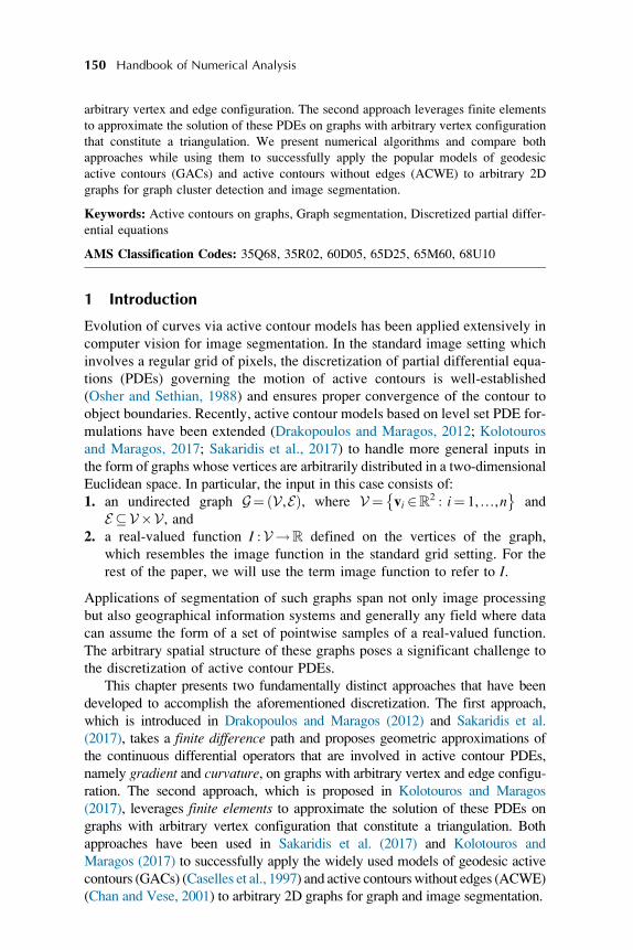
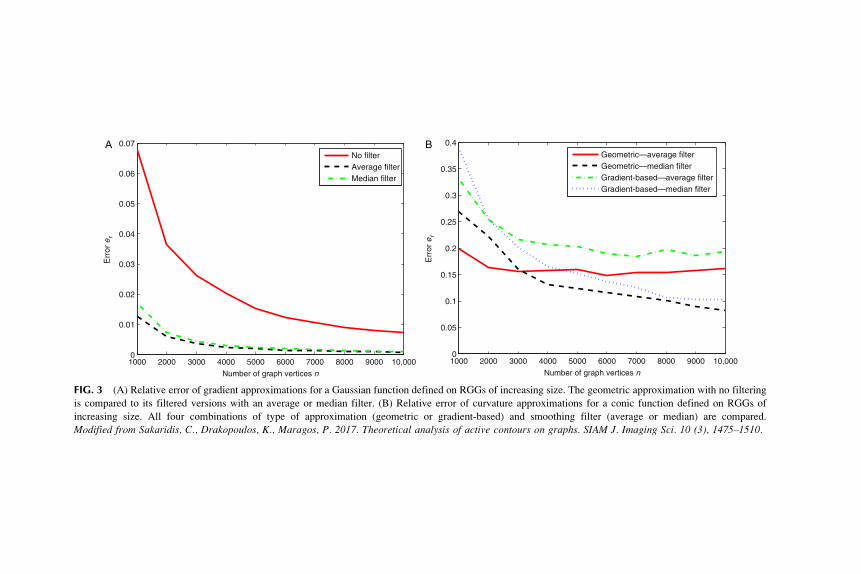
with σ ¼ 0.25 and x0 ¼ y0 ¼ 0.5. Fig. 3A shows average values of er over10 different graphs for each size to reduce variance in the reported perfor-

mance. Using either an average or a median filter reduces the relative error

substantially irrespective of size. Based on this result, smoothing filtering is

generally applied for gradient in practice when performing active contour

evolution.

Another practical consideration about the geometric gradient approxima-

tion (7) is that its absolute error increases as the magnitude of the true gradient

grows large, i.e., when the function exhibits abrupt variations. This does not

pose a problem for the calculation of gradient direction (which is relevant

as input for approximating the curvature), since the latter does not depend

on the range of the function’s variation around the examined vertex. Utilizing

all incident edges in the weighted sum of (7) ensures that all available infor-

mation in the neighbourhood of the vertex is used to estimate which direction

the gradient points to, as emphasized in Drakopoulos and Maragos (2012).

However, the estimated gradient magnitude with the geometric gradient

approximation (7) is prone to greater error, as it depends on the range of

the function’s variation. The use of difference quotients in (7) accentuates this

effect for dense graphs, where distances between neighbouring vertices that

appear in the denominator of the quotients approach zero. Thus, the preferable

approximation for gradient magnitude in practice is the maximum absolute


1000 2000 3000 4000 5000 6000 7000 8000 9000 10,0000

0.01

0.02

0.03

0.04

0.05

0.06

0.07

Number of graph vertices n

Err

or er

Err

or er

No filterAverage filterMedian filter

1000 2000 3000 4000 5000 6000 7000 8000 9000 10,0000

0.05

0.1

0.15

0.2

0.25

0.3

0.35

0.4

Number of graph vertices n

Geometric—average filterGeometric—median filterGradient-based—average filterGradient-based—median filter

A B

FIG. 3 (A) Relative error of gradient approximations for a Gaussian function defined on RGGs of increasing size. The geometric approximation with no filtering

is compared to its filtered versions with an average or median filter. (B) Relative error of curvature approximations for a conic function defined on RGGs of

increasing size. All four combinations of type of approximation (geometric or gradient-based) and smoothing filter (average or median) are compared.

Modified from Sakaridis, C., Drakopoulos, K., Maragos, P. 2017. Theoretical analysis of active contours on graphs. SIAM J. Imaging Sci. 10 (3), 1475–1510.

difference of values of the function along edges that are incident on v,introduced in Drakopoulos and Maragos (2012):

ruðvÞk k� maxw2N ðvÞ

fjuðwÞ�uðvÞjg: (14)

3.2 Geometric curvature approximation on graphs

After having devised an approximation scheme for the gradient of an embed-

ding function, the next step is to build upon this scheme in order to estimate

the curvature of the level sets of this function. The difference from the gradi-

ent case is that the input gradient values for curvature approximation are

already approximate themselves, i.e., a cascaded approximation is attempted.

Therefore, the error in curvature approximation on a graph is expected to

accumulate compared to gradient approximation error on the same graph,

since the estimated curvature at a vertex inherits the error of the estimated

gradients at its neighbouring vertices.

3.2.1 Formulation

The geometric curvature approximation that is proposed in Sakaridis et al.

(2017) is based on the expression of curvature as the divergence of the unit

gradient field F¼ru= ruk k of the embedding function u:

κðvÞ¼ div FðvÞ, ruðvÞ 6¼ 0: (15)

The integral definition of divergence as

div FðvÞ¼ limS!fvg

IΓðSÞ

F � n d‘

Sj j(16)

can then be used as a basis for approximating curvature, where S is a region

with area Sj j and boundary Γ(S) and n is the outward unit normal to this

boundary. In Drakopoulos and Maragos (2012), the integral in (16) is approxi-

mated using a polygonal region to form a finite sum over the neighbours of

the vertex (as shown in Drakopoulos and Maragos (2012, p. 8)). However,

certain arrangements of the neighbours of the examined vertex can lead to

regions with ill-defined area, boundary and normals when using the approach

of Drakopoulos and Maragos (2012), which prevents the presentation of

theoretical guarantees for the convergence of this approach.

To tackle these problems, the geometric curvature approximation of

Sakaridis et al. (2017) employs the neighbour angles that were introduced

in Section 3.1, in order to define the region S in (16) in a more compact

and principled fashion. Let S(v, ρ, θ0, θ) be a circular sector centred at v, withradius ρ, occupying an angle θ > 0 and whose rightmost radius is in the direc-

tion θ0. For vertex v, S(v) is formed as a union of circular sectors, each of


them corresponding to a neighbour of v, as we show in Fig. 4A. More formally,

for each neighbour w of v, the respective circular sector is S(v, d(v, w), ω(w),Δϕ(w)). The area of S(v) can then be expressed as

SðvÞj j ¼XNi¼1

ΔϕðwiÞ2

d2ðv,wiÞ: (17)

The challenge imposed by this construction of S(v) is the choice of suitable

values for F along the boundary of this region, given only its values at

the locations of neighbours of v. The resulting boundary consists of arcs,

each of which contains a neighbour of v, and line segments which connect

these arcs. The proposed approximation fixes the value of F along each arc

at the geometric gradient approximation computed for the corresponding

neighbour w using (7), Fg(w). Moreover, for every line segment, the nor-

malized mean of the approximate values of F along the two neighbouring

arcs is used. The idea is again to use information from the closest vertex,

which should be more reliable. We visualize the described configuration

in Fig. 4B.

Using the above approximations, the line integral in (16) is substituted

with a sum of simple line integrals over single arcs and line segments, which

have closed analytical forms. If we denote the integral over the arc Ca(wi)

containing neighbour wi by Ia(wi) and the integral over the line segment Cl(wi)

that connects the arcs Ca(wi) and Ca(wi+1) by Il(wi), we obtain

IaðwiÞ¼ dðv,wiÞ FgðwiÞ � ðsinðωðwi+ 1ÞÞ� sinðωðwiÞÞ, cosðωðwiÞÞ� cosðωðwi+ 1ÞÞÞ(18)

w1

w2

w3

v

S(v)Δφ(w1)

Δφ(w2)

Δφ(w3)

A B

wi

v

n = evwi

n

n

n

n

Fg(wi)

Fg(wi)

Fg(wi)

Fg(wi)+Fg(wi+1)

‖Fg(wi)+Fg(wi+1)‖

Fg(wi+1)

FIG. 4 (A) Definition of region S(v) through the neighbour angles. (B) The profile of values

of Fg at a part of the boundary of S(v) which corresponds to neighbour wi of v. Modified from

Sakaridis, C., Drakopoulos, K., Maragos, P. 2017. Theoretical analysis of active contours on

graphs. SIAM J. Imaging Sci. 10 (3), 1475–1510.


and

IlðwiÞ¼ ðdðv,wi+ 1Þ�dðv,wiÞÞFgðwiÞ+Fgðwi+ 1ÞFgðwiÞ+Fgðwi+ 1Þ � ðsinðωðwi+ 1ÞÞ, � cosðωðwi+ 1ÞÞÞ:

(19)

The geometric approximation of curvature proposed in Sakaridis et al. (2017)

is given by

κðvÞ�

XNi¼1

IaðwiÞ+ IlðwiÞ

SðvÞj j :(20)

While there was no proof of convergence for the curvature approximation of

Drakopoulos and Maragos (2012), the geometric curvature approximation of

Sakaridis et al. (2017) is proved to converge in probability for RGGs, as in

the geometric gradient approximation case, although the conditions are stron-

ger for curvature. The full proof of the following Theorem 3 is given in the

Supplementary Material of Sakaridis et al. (2017).

Theorem 3. Let Gðn,ρðnÞÞ be an RGG embedded in D ¼ [0, 1]2, with ρðnÞ 2ω n�1=2� � \ o 1ð Þ and v a vertex of G. If u :2 ! is continuously differentia-

ble and ru(v) 6¼ 0, then the curvature approximation of (20) converges inprobability to κ(v).

An alternative, gradient-based curvature approximation is additionally pre-

sented in Sakaridis et al. (2017) by leveraging the differential definition of

divergence instead of the integral definition of (16). This gradient-based cur-

vature approximation is also proved to converge in probability for RGGs,

under slightly stricter conditions than the geometric curvature approximation.

3.2.2 Practical application

The neighbourhood-based smoothing filtering that has been introduced in

Section 3.1.4 is also applicable to the output of curvature approximations.

In this case, the same type of filter is applied both to the gradient estimates

before using them for computing curvature and to the final curvature esti-

mates. In Fig. 3B, we present the results of an experiment similar to that in

Fig. 3A, this time focusing on the curvature of a function that corresponds

to an elliptical cone and comparing average versus median filtering as well

as the geometric versus the gradient-based curvature approximation. The form

of this function is ffiffiffiffiffiffiffiffiffiffiffiffiffiffiffiffiffiffiffiffiffiffiffiffiffiffiffiffiffiffiffiffiffiffiffiffiffiffiffiðx� x0Þ2

α2+ðy� y0Þ2

β2

s, (21)


where α ¼ 0.4, β ¼ 0.3, x0 ¼ �0.25 and y0 ¼ 0.5. Median filtering is superior:

the median-filtered approximations exhibit lower error than the corresponding

average-filtered ones over almost the entire range of graph sizes (except for

the smallest sizes). More importantly, the relative error of median-filtered

curvature is strictly decreasing for increasing graph size both with the geomet-

ric and the gradient-based approximation, in contrast to the average-filtered

cases, where the error stops decreasing around 4000 vertices. Due to these

facts, median filtering is preferred for smoothing gradient and curvature. In

addition, the geometric approximation induces a consistently smaller error

than the gradient-based approximation.

3.3 Gaussian smoothing on graphs

Apart from the approximations of gradient and curvature, an additional ingre-

dient which is required in particular for the GACmodel (1) to operate on graphs

is the edge-dependent stopping function gwhich helps attract the active contourto salient boundaries. The function gð rIσk kÞ : + !½0, 1 is typically a

decreasing function of the gradient magnitude of a smoothed version Iσ of theoriginal image function I, where smoothing acts as a regularization to limit

the effect of small local variations on the evolution of the contour. For this

smoothing, Drakopoulos and Maragos (2012) propose a simple graph-based

isotropic Gaussian filter, which is improved in Sakaridis et al. (2017) with

two alternative formulations that both include normalization to account for

nonuniform spatial vertex configurations in the arbitrary graph setting.

The isotropic 2D Gaussian filter with standard deviation σ is defined as

GσðxÞ¼ 1

2πσ2exp � xk k2

2σ2

!: (22)

Smoothing is performed in Drakopoulos and Maragos (2012) via a simple

graph-based convolution of (22) with the image function:

IσðvÞ¼Xw2V

IðwÞGσðv�wÞ: (23)

The stopping function g is then calculated through the following formula:

gð rIσk kÞ¼ 1

1 +rIσk k2λ2

: (24)

However, the arbitrary graph setting introduces nonuniformities: in some

parts of the graph, the vertices might be distributed more densely than in other

parts. This implies that (23) will operate counter-intuitively, introducing var-

iations to the smoothed image in regions of the graph where the original

image function is constant. To demonstrate this behaviour, we use a simple

binary image of a disk, shown in Fig. 5A. The result of applying (23) on this

image is shown in Fig. 5B. Not only has the range of image values changed,


00.2

0.40.6

0.81

0

0.5

10

0.2

0.4

0.6

0.8

1

xy

I

00.2

0.40.6

0.81

0

0.5

10

1000

2000

3000

4000

5000

6000

B

xy

Is

00.2

0.40.6

0.81

0

0.5

10

0.2

0.4

0.6

0.8

1

xy

Is

00.2

0.40.6

0.81

0

0.2

0.4

0.6

0.8

10

0.5

1

xy

g

00.2

0.40.6

0.81

0

0.2

0.4

0.6

0.8

10.2

0.4

0.6

0.8

1

xy

g

00.2

0.40.6

0.81

0

0.2

0.4

0.6

0.8

10

0.5

1

xy

g

C

D

A

E F

FIG. 5 Comparison of methods for Gaussian smoothing and computation of stopping function g. The original image on the graph (a disk) is shown in (A). (B)

and (C) contain smoothed versions Iσ of the original image using simple Gaussian filtering (Drakopoulos and Maragos 2012) and normalized Gaussian filtering

(Sakaridis et al. 2017) respectively. (D), (E) and (F) contain results for g using the three compared methods, i.e., Gaussian derivative filtering with separate nor-

malization (Sakaridis et al. 2017), simple Gaussian filtering (Drakopoulos and Maragos 2012), and normalized Gaussian filtering (Sakaridis et al. 2017) respec-

tively. The results in (C), (D) and (F) are obtained using σ ¼ 0.02 and λ ¼ 0.05, while those in (B) and (E) are obtained using σ ¼ 0.05 and λ ¼ 1000. The

approximation of (14) is used to compute the gradient magnitude for simple Gaussian filtering and normalized Gaussian filtering. For all three methods,

rIσk k is filtered with a median filter before feeding it to (24) for computing g. Modified from Sakaridis, C., Drakopoulos, K., Maragos, P. 2017. Theoretical

analysis of active contours on graphs. SIAM J. Imaging Sci. 10 (3), 1475–1510.

but the interior of the original disk also exhibits significant variations in

image values. This shortcoming is propagated to rIσk k and g, as shown in

Fig. 5E. There is a deviation of g from the ideal value of 1 in the interior of

the disk and a variation in its values as well, which means that the gradient

of g is not equal to 0 in the interior of the disk as it should.

This issue is tackled in Sakaridis et al. (2017) by including a normalization

term in (23) to address nonuniformities:

IσðvÞ¼

Xw2V

IðwÞGσðv�wÞXw2V

Gσðv�wÞ : (25)

This method is termed normalized Gaussian filtering and its result for the

examined disk image is shown in Fig. 5C. The smoothed image is now similar

to the respective output of simple Gaussian filtering in the usual image pro-

cessing setting with a regular grid. As a result, the profile of the corresponding

g function (shown in Fig. 5F) meets expectations.

An alternative formulation of Gaussian smoothing proposed in Sakaridis

et al. (2017) is based on the fact that the input of the stopping function is

the gradient of the smoothed image rather than the smoothed image itself.

Since the derivatives of the Gaussian filter have closed analytical forms, it

is possible to exchange the convolution with the gradient operator and con-

volve the image directly with Gaussian derivatives in order to obtain the gra-

dient of Iσ without performing numerical approximations. In this case,

normalization is not straightforward as in normalized Gaussian filtering:

Gaussian derivatives assume both positive and negative values. This diffi-

culty is circumvented by splitting the vertices into two sets, according to the

sign of the Gaussian derivative with respect to the processed vertex, and

performing separate normalization for each of these sets. This separation

can be easily expressed in terms of the vertices’ coordinates. If we denote

v ¼ (v1, v2), then Gaussian derivative filtering with separate normalization

is defined as

rIσðvÞ

¼

Xw2V:w1�v1

IðwÞ∂Gσðv�wÞ∂x

Xw2V:w1�v1

∂Gσðv�wÞ∂x

+

Xw2V:w1<v1

IðwÞ∂Gσðv�wÞ∂x

�Xw2V:w1<v1

∂Gσðv�wÞ∂x

,

Xw2V:w2�v2

IðwÞ∂Gσðv�wÞ∂y

Xw2V:w2�v2

∂Gσðv�wÞ∂y

+

Xw2V:w2<v2

IðwÞ∂Gσðv�wÞ∂y

�Xw2V:w2<v2

∂Gσðv�wÞ∂y

0BBBBBBBBBBBBB@

1CCCCCCCCCCCCCA:

(26)

The result of Gaussian derivative filtering with separate normalization on

the examined disk image in Fig. 5D is at least as satisfactory as in the normal-

ized Gaussian filtering case of Fig. 5F and clearly superior to simple Gaussian

filtering of Drakopoulos and Maragos (2012).


4 Active contours on graphs using a finite element framework

4.1 Problem formulation and numerical approximation

In this section we will discuss a method for solving active contour evolution

equations on graphs using the finite element method as presented by

Kolotouros and Maragos (2017). Finite element analysis is a powerful frame-

work that enables us to solve complex PDEs in a simple and elegant manner.

The main difference between finite difference and finite element methods is that

the former try to approximate the differential operators by discretizing them

whereas the latter approximate the solution with functions belonging to finite

dimensional function spaces. This can be useful, especially in the case of small

graphs where the accurate approximation of differential operators is a challeng-

ing problem. Additionally, compared to finite differences, the finite element

method is more suitable for functions defined on irregular domains or for mod-

elling discontinuities. There is a number of works that attempt to apply the finite

element method for solving level set equations. The work in Mourad et al.

(2005) presented a finite element solution to the level set equation by enforcing

that the level set function remains a signed distance function throughout the evo-

lution. A solution to the problem that exploits the partition-of-unity property of

the finite element shape functions was proposed in Valance et al. (2008). A

generic finite element algorithm approach for solving the Hamilton–Jacobiand front propagation equation was developed in Barth and Sethian (1998).

In this section we will consider general active contour models that can be

modelled with level set equations of the form

FðuÞ∂u∂t

¼ div GðuÞruð Þ+HðuÞru � n ¼ 0 on the boundary ∂Ω

uðx,y,0Þ ¼ dist*ðx,yÞ,(27)

where F, G and H are functionals of u and dist*(x, y) is the signed distance

function from the initial curve. Popular active contour models that can be

expressed in the above form are

l Erosion/Dilation:

FðuÞ¼ 1

kru k , GðuÞ¼ 0, HðuÞ¼ c, (28)

l Geometric Active Contours:

FðuÞ¼ 1

g kru k , GðuÞ¼ 1

kru k , HðuÞ¼ 0, (29)

l Geodesic Active Contours:

FðuÞ¼ 1

kru k , GðuÞ¼ g

kru k , HðuÞ¼ β, (30)

where g(x, y) is the edge stopping function defined in (24).


The core of the Finite Element method is that it converts PDEs to integral

equations that can then be solved using function approximations. It can be

verified that using some simple manipulations, (27) can be converted to an

equivalent integral equationZZΩ

FðuÞ∂u∂tϕ dxdy¼�

ZZΩ

GðuÞru � rϕ dxdy +

ZZΩ

HðuÞϕ dxdy (31)

The above form is known as the weak form and it must hold for all functions

ϕ 2 H1(Ω). H1(Ω) is the Sobolev space consisting of all functions defined in

Ω whose first order derivatives—in the distributional sense—belong to L2(Ω).The previous steps did not involve any numerical approximation. The

original problem was converted to an integral form that is expected to be

equivalent to the original problem. Next, the solution will be approximated

using the Galerkin method. Another main idea of the finite element analysis

is that it does not discretize continuous differential operators using finite dif-

ferences but instead approximates the solution of the equations with functions

belonging to finite dimensional subspaces of H1(Ω). Let Vn be a

n-dimensional subspace of H1(Ω) and fϕigni¼1 a basis of Vn. The approximate

solution �u can be written as a linear combination of the basis functions and

since the problem is time-dependent, we allow the coefficients of the linear

combination to be functions of time. Thus we have

�uðx,y, tÞ¼Xni¼1

ciðtÞϕiðx,yÞ: (32)

We demand that (31) holds at least for all the functions that belong to the

subspace Vn. Since (31) is a linear functional in ϕ and fϕigni¼1 form a basis

of Vn, this is equivalent to demanding that it holds for each of the basis

functions ϕi. If we use the fact that

∂�u

∂tðx,y, tÞ¼

Xni¼1

_ciðtÞϕiðx,yÞ, (33)

and substitute in (31) we get

Xni¼1

_ci

ZZΩ

Fð�uÞϕiϕj dxdy¼�Xni¼1

ZZΩ

Gð�uÞrϕi � rϕj dxdy +

ZZΩ

Hð�uÞϕj, j¼ 1,…n:

(34)

This is a nonlinear system of ordinary differential equations (ODEs) that can

be written in the form

AðcÞ _c¼ bðcÞ, (35)

where A ¼ {Aij}is a n � n matrix that depends on c and b¼fbign1, c¼fcign1are n-dimensional vectors with


AijðcÞ¼AjiðcÞ¼ZZ

ΩFXnk¼1

ckϕk

!ϕiϕj dxdy, (36)

and

biðcÞ¼�Xnj¼1

ZZΩ

GXnk¼1

ckϕk

!rϕi � rϕj dxdy +

ZZΩ

HXnk¼1

ckϕk

!ϕi dxdy:

(37)

The initial condition for the above system of differential equations can be

obtained from the projection �uðx,y,0Þ of u(x, y, 0) onto the subspace Vn, i.e.,

�uðx,y,0Þ¼Xni¼1

huðx,y,0Þ,ϕiiϕi, (38)

and thus

cið0Þ¼ huðx,y,0Þ,ϕii, (39)

where h�,�iis the usual inner product defined on H1(Ω) with

hf ,gi¼ZZΩ

fg dxdy +

ZZΩ

rf � rg dxdy: (40)

Consider a graph GðV,EÞ. We assume that the graph has a total of n verti-

ces and each vertex vi is a point in Ω and can be described by its respective

planar coordinates (xi, yi). Note that every finite set of points in the plane

can be mapped into the unit square by applying a translation followed by a

scaling. Thus if we apply an appropriate geometrical transformation we can

map the set of vertices to a subset of Ω. For each vertex vi 2V we choose a

function ϕi that belongs to H1(Ω) with the following properties:

1. fϕigni¼1 are linearly independent, and

2. for any nonadjacent vertices vi, vj, suppðϕiÞ\ suppðϕjÞ¼ ;.We can see that the functions fϕigni¼1 form a basis of some subspace S of

H1(Ω). Also, for reasonably smooth functions ϕi, supp(rϕi)nsupp(ϕi) is a

null set and thus suppðrϕiÞ\ suppðrϕjÞ is also a null set. Thus we can con-

clude that if vi and vj are two nonadjacent vertices of G, then hϕi, ϕvi¼ 0 and thus

ϕi, ϕj are orthogonal.

Proposition 1. For any graph GðV,EÞ with vi ¼ (xi, yi) 2 Ω there is at leastone set of functions fϕigni¼1 with the properties 1 and 2.

For a proof of this fact we refer the reader to Kolotouros and Maragos (2017).

Next we will describe how we can obtain the solution of (35) on a graph

GðV,EÞ equipped with the functions fϕigni¼1. First, from (36) we can see that

Aij(c) ¼ 0 if vi is not a neighbour of vj. If the number of edges for each vertex


is small compared to the total number of vertices then A(c) is sparse. Addi-

tionally the summation in (37) reduces to a summation in the neighbourhood

of vi and thus

biðcÞ¼�X

vj2Ni[fvig

ZZΩ

GXnk¼1

ckϕk

!rϕi � rϕj dxdy+

ZZΩ

HXnk¼1

ckϕk

!ϕi dxdy,

(41)

where Ni is the neighbourhood of vertex vi.For the rest of the analysis the class of graphs will be restricted to the

family of Delaunay graphs and more specifically the case of Delaunay graphs

that are constructed from the Delaunay triangulation of a finite set of points in

the unit square. Delaunay triangulation is a method of dividing the convex hull

of a set points into triangles that tends to avoid creating sharp triangles, a prop-

erty that ensures good convergence results for the solution of PDEs. For more

details about the Delaunay triangulation and the algorithms used to produce it,

we refer the reader to Persson and Strang (2004). Images can be thought of as a

special case of Delaunay graphs with the vertices being the pixels of the image.

In the case of graphs, the image function I is defined as in Section 1, i.e., only

on the vertices of the graph. For the case of the image gradient rI, however,since we will be using numerical integration, it is more convenient to define

it as a 2D function defined on Ω. This function is piecewise constant in

each triangle of the triangulation and its value is the gradient of the plane

that is formed by the values of I in the three vertices of the triangle. Similarly,

g¼ gðkrIkÞ will also be constant in each triangle of the triangulation.

Let GðV,EÞ be a Delaunay graph and fTigmi¼1 the triangles of the Delaunay

triangulation. Kolotouros and Maragos (2017) approximate the solution with a

function belonging to the space of continuous functions on Ω which are linear

in each triangle of the triangulation. We will denote this space as Slin. More

formally

Slin ¼f f 2CðΩÞ : f jTi ¼ aix+ biy + ci, for i¼ 1,…,mg: (42)

This choice of subspace provides good convergence properties and also sim-

plifies calculations as we shall see later on. After the selection of the subspace

we have to choose a basis of Slin. A possible choice satisfying the aforemen-

tioned properties are the pyramid functions. For each vertex vi of the graph we

define the function ϕi as

l ϕi(vi) ¼ 1.

l ϕi(vj) ¼ 0, for j 6¼ i.l ϕi is linear in each triangle.

It is easy to verify that suppðϕiÞ\ suppðϕjÞ¼ ; if vi is not a neighbour of vjand ϕi 2 Slin. It can also be proven that fϕigni¼1 are linearly independent


and thus form a basis of Slin. In Fig. 6A we can see the form of the ϕi functions

for the case of a rectangular grid. With this choice we can see that ϕi overlaps

only with the six other ϕj that correspond to the vertices vj that are adjacent

to vi. Thus each row of A contains at most seven nonzero elements and

at the same time only seven different coefficients ci appear in these expres-

sions. We can think of ϕi as functions that interpolate discrete data in a

rectangular grid. Assume for example that we have samples of a 2D func-

tion f at n points (xi, yi) on the plane. By creating the Delaunay graph that cor-

responds to the above set of points we can construct a continuous function f thatapproximates f as

f ðx,yÞ¼XNi¼1

f ðxi,yiÞϕiðx,yÞ: (43)

From the above construction and the properties of ϕi, it is easy to verify that

f ðxi,yiÞ¼ f ðxi,yiÞ and in each triangle of the triangulation it essentially per-

forms a form of linear interpolation. In Fig. 6B we can see an example of

an interpolation of discrete data in a rectangular grid.

The final remaining step is the discretization in time. For a system of

ODEs we have several options for the approximation of derivatives, each

one with its advantages and disadvantages and the choice of a particular

method depends on the specific properties of each problem. We want to cal-

culate the solution in a subset of the time interval [0, +∞) starting from the

initial condition until we reach convergence. Let tk, k � 0 be the sequence

of time points at which we calculate the solution with t0 ¼ 0 and tk ¼ kΔt.Here we assume that we use a fixed time step Δt. Also with ck we will denotethe approximation of c(tk). Kolotouros and Maragos (2017) used the explicit

Euler method which approximates the time derivative with the forward

difference

A B

FIG. 6 (A) Pyramid function ϕi centred in node vi for a rectangular grid. (B) Interpolation of

discrete data in a 4 � 4 rectangular grid using the ϕi functions. With solid circles we represent

the original discrete data.


_cðtkÞ¼ ck + 1� ck

Δt: (44)

If we substitute this into (35) we obtain

AðckÞck + 1 ¼AðckÞck +Δt � ðckÞ: (45)

This reduces to solving a linear system for each time step. This method is easy

to implement but puts limits on the choice of time step Δt. It is necessary to

choose a very small time step—often in the order of 1/n2—to ensure that the

curve evolution is stable.

Kolotouros and Maragos (2017) also provide an analysis of the complexity

of the presented algorithm. For the sake of simplicity let us consider the case

of the Delaunay graphs that correspond to images, with the graph structure

depicted in Fig. 6A. We assume that we have a h �w image. The resulting

graph will have a total of n ¼ hw vertices. Since each row of A contains at

most seven nonzero elements, A(ck) can be computed in linear time in each

time step. Also due to its sparsity, matrix multiplication can be performed

in linear time. Observing that b(ck) can also be computed in linear time, the

right-hand side needs O(n) time in each step. With an appropriate node label-

ling, A(ck) takes the form of a band matrix with a band length of

minðh,wÞ¼Oð ffiffiffin

p Þ. For a n �n band matrix with band length d the solution

of a linear system needs O(nd2) operations. So O(n2) operations are required

in each time step, which is prohibitive for large images. As far as the time

evolution is concerned, the total number of steps until convergence cannot

be specified a priori, since it depends on the shape and position of the initial

curve. If the initial curve is close to the object boundaries, only a few time

steps are needed until convergence.

4.2 Locally constrained contour evolution

In this part we present an extension of the previous framework to solve curve

evolution models of the form

FðuÞ∂u∂t

¼ δEðuÞ div GðuÞruð Þ +HðuÞð Þru � n¼ 0 on the boundary ∂Ω

uðx,y,0Þ¼ dist*ðx,yÞ:(46)

where δE(x) is an approximation of the Dirac δ function, with δE ! δ, as E ! 0.

A typical choice for δE is the piecewise constant approximation

δEðxÞ¼ 1=E, jxj E,0, jxj> E

�: (47)

The term δE constrains the curve evolution in a small area near the current posi-

tion of the curve, i.e., the 0-level set. One popular active contour model that can

be represented using (46) is the ACWE model of Chan and Vese (2001).


The first part of the discussion will involve showing how (46) can be

approximated on graphs. Define the sets

U +t ¼fðx,yÞ 2V : uðx,y, tÞ> 0g, (48)

U�t ¼fðx,yÞ 2V : uðx,y, tÞ< 0g, (49)

U0t ¼fðx,yÞ 2V : uðx,y, tÞ¼ 0g: (50)

U +t , U�

t and U0t are the set of points that are outside, inside and on the curve at

time t. Also we define the set of active points at time t as

U�t ¼ ∂U +

t [∂U�t [ U0

t , (51)

where ∂S denotes the boundary of the set S�V and is defined by

∂S¼fv2 S : 9v0 2 VnS s:t: v0 � vg: (52)

The set of active points represent the points that are within “unit” distance

from the current position of the active contour. Fig. 7 depicts visually how

the active points are computed.

Then—up to a positive scaling factor—δE(u) can be approximated on G at

time t with

δGt ðvÞ�1, if v2U�

t

0, elsewhere:

�(53)

Using the above definition, the evolution equation for (46) can be approxi-

mated as~AðcÞ _c¼ ~bðcÞ, (54)

FIG. 7 Illustration of active points for a Delaunay graph with 100 vertices. Blue nodes: Verticesoutside the contour. Black nodes: Vertices inside the contour. Yellow nodes: Vertices on the con-

tour. Nodes with red boundary: Active points.


where ~AðcÞ is a n � n matrix with

~AijðcÞ¼AijðcÞ, if vi 2U�

t

1, if vi 62 U�t and j¼ i

0, elsewhere

8<: ,

and ~bðcÞ a n-dimensional vector with

~biðcÞ¼biðcÞ, if vi 2U�

t

0, elsewhere

�: (55)

It is easy to observe that for all nonactive vertices vi, _ci ¼ 0 and thus the curve

evolution is indeed constrained at the subset U�t .

The above formulation will help us reduce significantly the computational

complexity of each time step. Consider the explicit Euler approximation of (54)

~AðckÞ ck + 1� ckð Þ¼Δtk~bðckÞ: (56)

For all vertices vi that are not in the set of active points (ci)k+1 �(ci)k ¼ 0. So,

for all vi 2U�t , (ci)k+1 does not depend on the values (cj)k, where vj 62 U�

tk. Thus

the corresponding values Aij(ck) have no influence on the solution of the lin-

ear system, so they can be set to 0. Let A�k be a jU�

tkj� jU�

tkj submatrix of

~AðckÞ that is constructed by keeping only the elements Aij with vi and

vj 2U�tk. Similarly b�k is a jU�

t j-dimensional vector that is derived from b(ck)

by discarding all the elements vi with vi 62 U�t . If we set Δck ¼ ck+1 �ck

and Δc�k ¼ I�kΔck, where Ik is the jU�tkj�n projection matrix with Iii ¼ 1 and

Iij ¼ 0 if i 6¼ j then we get the equivalent linear system

A�kΔc�k ¼Δtkb�k : (57)

After computing Δck from (57) the update rule for the coefficients c in matrix

notation becomes

ck + 1 ¼ ck + ITkΔc�k : (58)

Most level set evolution models require reinitialization of the embedding

function to ensure correct results and there have been several approaches to

alleviate this need, as in Li et al. (2005). In this framework we avoid the need

for reinitialization in an indirect way; to ensure the stability of the numerical

method and make it possible to use large time steps, we normalize the embed-

ding function after each time step. Specifically, �uðx,y, tÞ and consequently the

vector of coefficients ck is saturated outside the interval [�r, r]. A typical

choice of r is r¼ max ju0ðx,yÞjor equivalently r¼ max jc0j. With the use of

normalization we can choose a time step Δtk �1/n, which is significantly

larger than the time step used for the solution of (27). A similar approach can-

not be adopted for the solution of the full evolution equation because in each


time step the evolution domain covers the whole graph and although the

embedding function will be bounded, large time steps will produce noisy

artifacts.

As in the previous section, Kolotouros and Maragos (2017) provide an

estimate for the computational complexity of the proposed algorithm for the

case of Delaunay graphs that correspond to images. For a h �w image with

n pixels, each of U +tk, U�

tkand U0

tkis the union of a number of 1D curves. Gen-

erally, typical 1D curves in an image grid with n pixels contain Oð ffiffiffin

p Þ pixels.Thus, in almost all practical cases U�

tkwill contain Oð ffiffiffi

np Þ pixels. Since the

number of edges in the planar Delaunay graph is bounded by 3n �6, a naive

calculation of U�tkusing the definitions of its components requires O(n) opera-

tions. Additionally, it is easy to verify that given the set of active points, the

elements of Ak* and bk* can be computed in O(n) time. Since A(ck) is a

sparse band matrix, Ak* will also be a band matrix, but its band length can

often be OðjU�tkjÞ. However, using the Reverse Cuthill–McKee algorithm

(George and Liu, 1981) which can be implemented in OðjU�tkjÞ time we can

obtain a permuted matrix with a band length of OðffiffiffiffiffiffiffiffiffijU�

tkj

qÞ on average. Thus

the solution of the constrained linear system is expected to require O(n) opera-tions. Consequently, we have shown that on average, each time step of the

algorithm requires O(n) operations. If we compare this result with the number

of operations required for the full curve evolution, we can see that the con-

strained curve evolution algorithm is faster by an order of magnitude. Its lin-

ear complexity with respect to the number of graph vertices makes it feasible

to be used in practical applications.

These results point towards a fast implementation of general active con-

tour models that can take the form of (27). The level set-based approach

enables us to handle topological changes in the curve in a solid and efficient

manner, but introduces an extra computational burden, because we have to

evolve a 2D function instead of a curve. The answer to this problem is to

try to limit our focus in a small area of interest near the curve—often

referred as band—and evolve the embedding function in this subset of the

image. Similar methods, called narrow-band methods, were described for

the case of images in Adalsteinsson and Sethian (1995), Whitaker (1998)

and Peng et al. (1999). Instead of evaluating the curve evolution on the

whole graph, the curve evolution is constrained in a small band near the

curve. This approximation is based on the assumption that the embedding

function evolves in such a way that points outside or inside the curve will

not change status, at least until the moment that the active contour reaches

them. The above assumption is valid for the majority of active contour meth-

ods, such as simple Erosion/Dilation as well as the Geometric and Geodesic

Active Contours.


5 Experimental results

Using the graph-based approximations of the main differential terms of active

contour models with level sets, Sakaridis et al. (2017) apply finite difference-

based algorithms to solve the respective PDEs that define these models on

arbitrary graphs. The input comprises a graph G¼ ðV,EÞ and an image func-

tion I, as specified in Section 1. The two representative active contour models

which are used to develop these algorithms are the GAC model (Caselles

et al., 1997) presented in (1) and the ACWE model (Chan and Vese, 2001)

presented in (2). We first present the GAC algorithm and corresponding

results and then proceed to ACWE.

The finite difference algorithm of Sakaridis et al. (2017) for GACs on

graphs includes the following steps:

1. Compute gð rIσk kÞ, using either (25) and (14) or (26) to compute rIσk k.In both cases, median filtering is applied to rIσk k before plugging it into

(24) for computing g. Then, compute the magnitude of g’s gradient using(14) and its direction using (7).

2. Choose a subset X of V which contains the objects to be segmented and

initialize the embedding function with the signed distance function from

the boundary of X, denoted by u0. By convention, u0 is positive inside X.3. Iterate for r 2

ur ¼ ur�1 +Δtððκ� cÞ rur�1k kg+rg � rur�1Þ (59)

until convergence. In the difference equation (59), Δt and c are positive con-

stants and κ is the estimated curvature of the level sets of ur�1 using (20). The

direction of rur�1 is computed with (7) and its magnitude with (14). Median

filtering is applied both to κ and rur�1 before using them in (59).

In practice, after each iteration of step 3 of the algorithm, ur is smoothed with

a median filter before proceeding to the next iteration. The parameters

involved in the algorithm are the time step Δt of the difference equation,

the balloon force constant c, the scale σ of the Gaussian smoothing filter

and parameter λ of the stopping function g (24). Tuning their values depend-

ing on the input at hand is pivotal in obtaining satisfactory segmentation

results. In the following experiments of Section 3, Δt ¼ 0.005 and c ¼ 2 unless

otherwise specified.

A simple analysis of the computational complexity of each iteration (59)

of the algorithm by examining each term on the right-hand side of (59) and

aggregating the individual contributions of all terms shows that the total com-

plexity of each iteration is Θ(n + m), which is linear in the number of vertices

and in the number of edges.

We first discuss and experimentally explore the practical aspect of graph

construction when applying such graph-based algorithms on arbitrarily spaced

data as well as regular pixel grids. In the case of arbitrary graphs, the raw


input often consists only of V and I, without any information about the edges.

This setting leaves us free to choose the type of edge structure of the graph.

Sakaridis et al. (2017) experiment with two types: RGGs and Delaunay trian-

gulations (DTs) ( Jaromczyk and Toussaint, 1992). In the case of regular

images on a grid, graph-based active contour methods are still relevant, since

the input image can be sampled at a number of arbitrary locations that will

serve as the vertices. This brings us to the previous setting where edges can

be defined freely. A baseline for such sampling is to place vertices uniformly

at random on the image domain. A more sophisticated strategy is to extract

vertex locations via watershed transformation. In particular, watershed trans-

formation is applied directly to the gradient of the image and the vertices

are placed at the centroids (ultimate erosions) of the resulting superpixels.

For the grayscale image with four distinct coins in Fig. 8A, we compare the

results of the GAC algorithm of Sakaridis et al. (2017) for all four possible

combinations of the aforementioned vertex placement strategies (random,

watershed) and choices of edge structure (RGG, DT) in Fig. 8C–F. To ensure

a fair comparison, the number of randomly placed vertices is approximately

the same as in the watershed case. The most accurate segmentation is

achieved with DT and watershed-placed vertices (Fig. 8F). Moreover, DT

consistently outperforms RGG and watershed-based vertex placement outper-

forms random placement. Consequently, the DT edge structure is preferable to

the random geometric one and usage of watershed transformation to place

vertices when a full image is available is preferable to random placement,

as it captures image particularities into the spatial structure of the graph. In

the rest of the experiments of Sakaridis et al. (2017) that are presented in this

section, construction of the graphs follows these choices.

Fig. 9 presents results of the algorithm of Sakaridis et al. (2017) for GACs

on graphs on two natural colour images coming from the Berkeley Segmenta-

tion Dataset BSDS500 (Martin et al., 2001). The images were converted to

grayscale for applying the algorithm. In general, the algorithm segments the

dominant objects in the images successfully, even though background clutter

and thin protrusions or concavities of the objects’ boundaries sometimes cause

minor inaccuracies.

An interesting application of the examined graph segmentation framework

is related to geographical data, where the two spatial coordinates are longitude

and latitude and the image function can encode information about any type of

real-valued signal defined at the vertices of the graph. Such a signal is the sig-

nal strength of a cellular network, such as that shown in Fig. 10A. The coor-

dinates and the values of signal strength are normalized and a very small time

step Δt ¼ 10�4 is used to guarantee convergence, which requires more itera-

tions until termination than in the previous experiments. Other parameters are

set as σ ¼ 0.03, λ ¼ 0.02 and c ¼ 20. The segmented set of vertices in

Fig. 10D using the GAC algorithm of Sakaridis et al. (2017) comprises two


050

100150

200250

300

0

50

100

A B C

D E F

150

200

00.5

1

x

y

I

FIG. 8 Segmentation of grayscale objects on graphs with the GAC algorithm of Sakaridis et al. (2017). (A) Full grayscale image with four coins (B) image function on

watershed-based DT (C)–(F) final segmentation results overlaid on original image, with segmented objects shown in red and background in blue. We use (C) randomly placed

vertices with random geometric structure, σ ¼ 0.02 and λ ¼ 0.03, (D) randomly placed vertices with DT structure, σ ¼ 0.02 and λ ¼ 0.03, (E) watershed-placed vertices with

random geometric structure, σ ¼ 0.008 and λ ¼ 0.07, and (F) watershed-placed vertices with DT structure, σ ¼ 0.01 and λ ¼ 0.07. The total number of iterations to obtain the

final segmentation result is (C) 2200, (D) 4000, (E) 3000 and (F) 4000.Modified from Sakaridis, C., Drakopoulos, K., Maragos, P. 2017. Theoretical analysis of active contours

on graphs. SIAM J. Imaging Sci. 10 (3), 1475–1510.

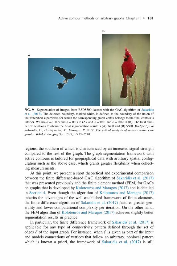
regions, the southern of which is characterized by an increased signal strength

compared to the rest of the graph. The graph segmentation framework with

active contours is tailored for geographical data with arbitrary spatial config-

uration such as the above case, which grants greater flexibility when collect-

ing measurements.

At this point, we present a short theoretical and experimental comparison

between the finite difference-based GAC algorithm of Sakaridis et al. (2017)

that was presented previously and the finite element method (FEM) for GACs

on graphs that is developed by Kolotouros and Maragos (2017) and is detailed

in Section 4. Even though the algorithm of Kolotouros and Maragos (2017)

inherits the advantages of the well-established framework of finite elements,

the finite difference algorithm of Sakaridis et al. (2017) features greater gen-

erality and lower computational complexity per iteration. On the other hand,

the FEM algorithm of Kolotouros and Maragos (2017) achieves slightly better

segmentation results in practice.

In particular, the finite difference framework of Sakaridis et al. (2017) is

applicable for any type of connectivity pattern defined through the set of

edges E of the input graph. For instance, when E is given as part of the input

and models connections of vertices that follow an arbitrary, nonlocal pattern

which is known a priori, the framework of Sakaridis et al. (2017) is still

A

B

FIG. 9 Segmentation of images from BSDS500 dataset with the GAC algorithm of Sakaridis

et al. (2017). The detected boundary, marked white, is defined as the boundary of the union of

the watershed superpixels for which the corresponding graph vertex belongs to the final contour’s

interior. We use σ ¼ 0.005 and λ ¼ 0.03 in (A), and σ ¼ 0.01 and λ ¼ 0.02 in (B). The total num-

ber of iterations to obtain the final segmentation result is (A) 3400 and (B) 5600. Modified fromSakaridis, C., Drakopoulos, K., Maragos, P. 2017. Theoretical analysis of active contours on



0 0.2 0.4 0.6 0.8 1 1.2 1.4 1.6 1.80

0.2

0.4

0.6

0.8

1A B

C D

0

0.2

0.4

0.6

0.8

1

0 0.2 0.4 0.6 0.8 1 1.2 1.4 1.6 1.80

0.2

0.4

0.6

0.8

1

0.2

0.4

0.6

0 0.2 0.4 0.6 0.8 1 1.2 1.4 1.6 1.80

0.2

0.4

0.6

0.8

1

0 0.2 0.4 0.6 0.8 1 1.2 1.4 1.6 1.80

0.2

0.4

0.6

0.8

1

0 0.2 0.4 0.6 0.8 1 1.2 1.4 1.6 1.80

0.2

0.4

0.6

0.8

1

FIG. 10 Segmentation of signal strength data of a cellular network on a graph with the GAC algorithm of Sakaridis et al. (2017). (A) Normalized data on graph.

(B) Smoothed signal strength. (C) Initial contour. (D) Final segmentation result after 40,000 iterations, with vertices in the contour’s interior shown in red and the

rest in blue. From Sakaridis, C., Drakopoulos, K., Maragos, P. 2017. Theoretical analysis of active contours on graphs. SIAM J. Imaging Sci. 10 (3), 1475–1510.

relevant. On the contrary, the FEM framework of Kolotouros and Maragos

(2017) only applies to triangulations; notably, it cannot handle the aforemen-

tioned case with arbitrary edge structure, or other commonly used types of

graphs such as k nearest neighbour graphs or RGGs. Furthermore, in the case

of triangulations, the complexity of each iteration of the finite difference-

based GAC algorithm is O(n), i.e., linear in the number of vertices n (which

follows from the general Θ(n + m) complexity and planarity of triangulations),

whereas the respective complexity of each iteration of the FEM-based GAC

algorithm is O n2ð Þ, i.e., quadratic in n.In Fig. 11 we compare the two approaches on the coins image and an

image from BSDS500 (Martin et al., 2001). The graphs are formed as

DTs with watershed-placed vertices. Whenever possible, we use the same

or at least similar parameter values for the two approaches, so that a fair

comparison is ensured. The results of the finite difference GAC algorithm

are presented in Fig. 11A and C and the respective results of the FEM

GAC algorithm are presented in Fig. 11B and D. The two methods demon-

strate similar overall performance on both images, with the FEM algorithm

producing slightly more accurate boundaries in challenging cases such as

the bird’s tail.

A

C D

B

FIG. 11 Comparison between the finite difference GAC algorithm of Sakaridis et al. (2017) and

the FEM GAC algorithm of Kolotouros and Maragos (2017). For the coins image, the foreground

is shown in red and the background in blue and we use σ ¼ 0.01 and λ ¼ 0.07 for both methods.

(A) The result of Sakaridis et al. (2017) after 4000 iterations. (B) The result of Kolotouros and

Maragos (2017) after 301 iterations, using c ¼ 10 and Δt ¼ 0.001. For the bird image, the

detected boundary is marked white and we use σ ¼ 0.005 for both methods. (C) The result of

Sakaridis et al. (2017) after 4400 iterations, using λ ¼ 0.05. (D) The result of Kolotouros and

Maragos (2017) after 4001 iterations, using λ ¼ 0.07, c ¼ 10 and Δt ¼ 0.001. From Sakaridis, C.,Drakopoulos, K., Maragos, P. 2017. Theoretical analysis of active contours on graphs. SIAM J.

Imaging Sci. 10 (3), 1475–1510.


We now proceed to the presentation of the ACWE algorithm of Sakaridis

et al. (2017) and related results. The finite difference algorithm of Sakaridis

et al. (2017) for ACWE on graphs includes the following steps:

1. Choose a subset X of V and initialize the embedding function with the

signed distance function from the boundary of X, denoted by u0. By con-

vention, u0 is positive inside X.2. Iterate for r 2:

c1 ¼ average IðvÞ : ur�1ðvÞ� 0f g, c2 ¼ average IðvÞ : ur�1ðvÞ< 0f g, (60)

ur ¼ ur�1 +Δt δE ur�1ð Þ μκ�ν� λ1 I� c1ð Þ2 + λ2 I� c2ð Þ2� ��

(61)

until convergence. In the difference equation (61), Δt, E, μ, ν, λ1 and λ2 are

positive constants and κ is the estimated curvature of the level sets of ur�1

using (20). Moreover, δE is the derivative of a regularized version of the

Heaviside function which was introduced in Chan and Vese (2001) as:

δEðxÞ¼H0EðxÞ¼

1

21 +

2

πarctan

x

E

� � 0¼ Eπ x2 + E2ð Þ : (62)

The standard ACWE model is modified in Sakaridis et al. (2017) for colour

images, so that it uses all three colour channels instead of reducing the image

to a simpler grayscale version. In order for the averages and Euclidean dis-

tances to be meaningful, the original RGB values of the vector-valued image

function I at graph vertices are transformed to CIELAB values, as the latter

colour space is more perceptually uniform. The update equations are modified

to operate on multiple colour channels:

c1 ¼ average IðvÞ : ur�1ðvÞ� 0f g, c2 ¼ average IðvÞ : ur�1ðvÞ< 0f g (63)

and

ur ¼ ur�1 +Δt δE ur�1ð Þ μκ�ν� λ1 I� c1k k2 + λ2 I� c2k k2� ��

: (64)

In Fig. 12, we present results that are analogous to Figs. 8F and 9A and

B by replacing the GAC algorithm with the ACWE algorithm and demon-

strate the utility of the geometric approximations proposed in Sakaridis

et al. (2017) for successfully translating various active contour models

to graphs. For the colour images from BSDS500 in Fig. 12A and C, the

modification of ACWE in (63) and (64) is used. The segmentation results

are of high quality, e.g., capturing the thin feathers at the eagle’s wing very

precisely.

Last we present some additional qualitative results when applying the

FEM framework for solving more complicated active contour models.

Kolotouros and Maragos (2017) presented Region-based Geodesic Active

Contours (RBGAC), an interactive segmentation algorithm where the users

have to specify some initial markers for the foreground and background and


then the algorithm iterates between expanding and shrinking contours to com-

pute the segmentation. An example use of this method can be seen in Fig. 13.

Also in Fig. 14 we depict a quantitative comparison between RBGAC and

several other popular interactive segmentation algorithms.

A

B

C

FIG. 12 Segmentation of images with the ACWE algorithm of Sakaridis et al. (2017). (A) and

(C) Images from BSDS500 with detected boundaries marked white. (B) Coins image with

detected foreground shown in red and background in blue. We use Δt ¼ 0.05, ν ¼ 0, λ1 ¼λ2 ¼ 1 and E¼medianvw2Efdðv,wÞg in all cases, μ ¼ 0.1 in (A) and μ ¼ 0.5 in (B) and (C).

The total number of iterations to obtain the final segmentation result is (A) 1000, (B) 7000 and

(C) 2000. Modified from Sakaridis, C., Drakopoulos, K., Maragos, P. 2017. Theoretical analysis

of active contours on graphs. SIAM J. Imaging Sci. 10 (3), 1475–1510.

FIG. 13 Illustration of RBGAC algorithm. Left column: Images and seeds. The red curves arethe initial contours and the blue polygons mark the regions of interest. Right column: Segmenta-

tion results.


6 Conclusion

In this chapter, we have delineated two approaches to translate level set-based

active contour models to the general case of arbitrary graphs, using either

finite differences (Drakopoulos and Maragos, 2012; Sakaridis et al., 2017)

or the finite element method (Kolotouros and Maragos, 2017) for the required

discretization of the employed PDEs. We have overviewed the approxima-

tions introduced in Sakaridis et al. (2017) for the gradient and curvature terms

in active contour models for 2D graphs with arbitrary vertex and edge config-

uration and presented the main theoretical results of Sakaridis et al. (2017)

regarding asymptotic consistency and accuracy of these approximations for

the class of random geometric graphs. In addition, a detailed presentation of

the formulation of the finite element method that is proposed in Kolotouros

and Maragos (2017) for the approximate solution of active contour PDEs

through discretization on arbitrary 2D Delaunay triangulations has been

provided. The effectiveness of the two examined methods has been demon-

strated experimentally by using them to apply the popular GAC and ACWE

models on regular as well as arbitrary graphs and successfully segment regular

images as well as unorganized 2D geographical data.

Although the framework of Sakaridis et al. (2017) applies to any type of

graph, the presented theoretical analysis considers random geometric graphs,

FIG. 14 Segmentation results. Columns 1–5: GrabCut Dataset. Columns 6–9: PASCAL Dataset.

From top to bottom: Ground Truth, segmentation results from GrabCut, Laplacian Coordinates,

Power Watershed, ACWE and RBGAC. Data from Kolotouros, N., Maragos P. 2017. A finite

element computational framework for active contours on graphs. ArXiv e-prints 1710.04346.


whose definition simplifies convergence proofs for the proposed approxima-

tions. However, judging from segmentation quality, more regular graph struc-

tures, such as Delaunay triangulations, lead to more accurate results. Therefore,

an interesting direction in this line is the theoretical study of the approximations

of Sakaridis et al. (2017) on graphs formed as Delaunay triangulations, ideally

establishing similar asymptotic consistency results to those shown in Sakaridis

et al. (2017).

Last but not least, both methods (Kolotouros and Maragos, 2017;

Sakaridis et al., 2017) are formulated for the case of 2D graphs. While this

type of input is sufficient to model signals such as regular images and geo-

graphical profiles, there are several areas of application that involve signals

defined in higher-dimensional—often 3D—Euclidean spaces, including

medical image processing and geology. Thus, it is worth generalizing the

above methods to more dimensions. For the approach of Sakaridis et al.

(2017) in particular, this requires generalizing the approximation formulae

for gradient and curvature. With regard to gradient, the main challenge is

the calculation of neighbour angles (cf. (5)) in higher dimensions. For each

vertex v, this would involve the calculation of solid angles which are

induced by the Voronoi tessellation of the ambient d-dimensional space that

is defined by the set of neighbours NðvÞ, analogously to Fig. 1. The general

formula of Ribando (2006) for measuring simplicial solid angles in Euclid-

ean spaces of arbitrary dimensionality would likely have to be utilized to

this end. As far as curvature is concerned, the quantity of interest is the

mean curvature and we foresee that the geometric type of approximation

we highlighted in Section 3.2 will require meticulous calculations in order

to be extended to more dimensions, whereas the gradient-based approxima-

tion we briefly mentioned, which uses the differential definition of diver-

gence, is easier to extend.

References

Adalsteinsson, D., Sethian, J.A., 1995. A fast level set method for propagating interfaces. J. Comput.

Phys. 118 (2), 269–277. ISSN 0021-9991. https://doi.org/10.1006/jcph.1995.1098.

Arias-Castro, E., Pelletier, B., Pudlo, P., 2012. The normalized graph cut and Cheeger constant:

from discrete to continuous. Adv. Appl. Probab. 44 (4), 907–937.

Barth, T.J., Sethian, J.A., 1998. Numerical schemes for the Hamilton-Jacobi and level set equa-

tions on triangulated domains. J. Comput. Phys. 145 (1), 1–40.

Belkin, M., Niyogi, P., 2006. Convergence of Laplacian eigenmaps. In: Advances in Neural Infor-

mation Processing Systems (NIPS).

Bensoussan, A., Menaldi, J.-L., 2005. Difference equations on weighted graphs. J. Convex Anal.

12 (1), 13–44.

Bertozzi, A.L., Flenner, A., 2012. Diffuse interface models on graphs for classification of high

dimensional data. Multiscale Model. Simul. 10 (3), 1090–1118.

Bougleux, S., Elmoataz, A., Melkemi, M., 2009. Local and nonlocal discrete regularization on

weighted graphs for image and mesh processing. Int. J. Comput. Vis. 84, 220–236.


https://doi.org/10.1006/jcph.1995.1098

http://refhub.elsevier.com/S1570-8659(19)30015-8/rf0015












Boykov, Y., Kolmogorov, V., 2003. Computing geodesics and minimal surfaces via graph cuts.

In: Proc. Int. Conf. Comput. Vis.

Boykov, Y., Veksler, O., Zabih, R., 2001. Fast approximate energy minimization via graph cuts.

IEEE Trans. Pattern Anal. Mach. Intell. 23 (11), 1222–1239.

Caselles, V., Catt�e, F., Coll, T., Dibos, F., 1993. A geometric model for active contours in image

processing. Numer. Math. 66, 1–31.

Caselles, V., Kimmel, R., Sapiro, G., 1997. Geodesic active contours. Int. J. Comput. Vis.

22 (1), 61–79.

Chan, T.F., Vese, L.A., 2001. Active contours without edges. IEEE Trans. Image Process. 10 (2),

266–277.

Chan, T.F., Esedoglu, S., Nikolova, M., 2006. Algorithms for finding global minimizers of image

segmentation and denoising models. SIAM J. Appl. Math. 66 (5), 1632–1648.

Chung, S.-Y., Berenstein, C.A., 2005. ω-Harmonic functions and inverse conductivity problems

on networks. SIAM J. Appl. Math. 65 (4), 1200–1226.

Couprie, C., Grady, L., Najman, L., Talbot, H., 2011a. Power watershed: a unifying graph-based

optimization framework. IEEE Trans. Pattern Anal. Mach. Intell. 33 (7), 1384–1399.

Couprie, C., Grady, L., Talbot, H., Najman, L., 2011b. Combinatorial continuous maximum flow.

SIAM J. Imaging Sci. 4 (3), 905–930.

Couprie, C., Grady, L., Najman, L., Pesquet, J.-C., Talbot, H., 2013. Dual constrained TV-based

regularization on graphs. SIAM J. Imaging Sci. 6 (3), 1246–1273.

Courant, R., Friedrichs, K., Lewy, H., 1967. On the partial differential equations of mathematical

physics. IBM J. Res. Dev. 11 (2), 215–234.

Cousty, J., Bertrand, G., Najman, L., Couprie, M., 2009a. Watershed cuts: minimum spanning for-

ests and the drop of water principle. IEEE Trans. Pattern Anal. Mach. Intell. 31 (8),

1362–1374.

Cousty, J., Najman, L., Serra, J., 2009b. Some morphological operators in graph spaces. In: Proc.

International Symposium on Mathematical Morphology.

Cousty, J., Bertrand, G., Najman, L., Couprie, M., 2010. Watershed cuts: thinnings, shortest path

forests, and topological watersheds. IEEE Trans. Pattern Anal. Mach. Intell. 32 (5), 925–939.

Desquesnes, X., Elmoataz, A., L�ezoray, O., 2013. Eikonal equation adaptation on weighted

graphs: fast geometric diffusion process for local and non-local image and data processing.

J. Math. Imaging Vision 46 (2), 238–257.

Drakopoulos, K., Maragos, P., 2012. Active contours on graphs: multiscale morphology and

graphcuts. IEEE J. Sel. Topics Signal Process. 6 (7), 780–794.

Elmoataz, A., L�ezoray, O., Bougleux, S., 2008. Nonlocal discrete regularization on weighted

graphs: a framework for image and manifold processing. IEEE Trans. Image Process.

17 (7), 1047–1060.

Elmoataz, A., Toutain, M., Tenbrinck, D., 2015. On the p-Laplacian and ∞-Laplacian on graphs

with applications in image and data processing. SIAM J. Imaging Sci. 8 (4), 2412–2451.

Elmoataz, A., Lozes, F., Toutain, M., 2017. Nonlocal PDEs on graphs: from tug-of-war games to

unified interpolation on images and point clouds. J. Math. Imaging Vision 57 (3), 381–401.

Garcı́a Trillos, N., Slep�cev, D., 2016. Continuum limit of total variation on point clouds. Arch.

Ration. Mech. Anal. 220 (1), 193–241.

George, A., Liu, J.W.H., 1981. Computer Solution of Large Sparse Positive Definite Systems.

Prentice Hall.

Gilboa, G., Osher, S., 2007. Nonlocal linear image regularization and supervised segmentation.

Multiscale Model. Simul. 6 (2), 595–630.






















































Gilboa, G., Osher, S., 2008. Nonlocal operators with applications to image processing. Multiscale

Model. Simul. 7 (3), 1005–1028.

Grady, L., 2006. Random walks for image segmentation. IEEE Trans. Pattern Anal. Mach. Intell.

28 (11), 1768–1783.

Grady, L., Alvino, C., 2009. The piecewise smooth Mumford-Shah functional on an arbitrary

graph. IEEE Trans. Image Process. 18 (11), 2547–2561.

Grady, L., Polimeni, J., 2010. Discrete Calculus: Applied Analysis on Graphs for Computational

Science. Springer Science & Business Media.

Heijmans, H.J.A.M., Nacken, P., Toet, A., Vincent, L., 1992. Graph morphology. J. Vis. Com-

mun. Image Represent. 3 (1), 24–38.

Hirani, A. N., 2003. Discrete Exterior Calculus (Ph.D. dissertation). Cal. Tech.

Jaromczyk, J.W., Toussaint, G.T., 1992. Relative neighborhood graphs and their relatives. Proc.

IEEE 80 (9), 1502–1517.

Kass, M., Witkin, A., Terzopoulos, D., 1988. Snakes: active contour models. Int. J. Comput. Vis.

1 (4), 321–331.

Kolotouros, N., Maragos, P., 2017. A finite element computational framework for active contours

on graphs. ArXiv e-prints 1710.04346.

Lee, D.D., Seung, H.S., 2001. Algorithms for non-negative matrix factorization. In: Advances in

Neural Information Processing Systems (NIPS).

L�ezoray, O., Grady, L., 2012. Image Processing and Analysis with Graphs: Theory and Practice,

Digital Imaging and Computer Vision, CRC Press.

L�ezoray, O., Elmoataz, A., Ta, V.-T., 2012. Nonlocal PdEs on graphs for active contours models

with applications to image segmentation and data clustering. In: ICASSP, pp. 873–876.

Li, C., Xu, C., Gui, C., Fox, M.D., 2005. Level set evolution without re-initialization: a new vari-

ational formulation. In: Proceedings of the IEEE Conference on Computer Vision and Pattern

Recognition (CVPR’05).

Lozes, F., Elmoataz, A., L�ezoray, O., 2014. Partial difference operators on weighted graphs for

image processing on surfaces and point clouds. IEEE Trans. Image Process. 23 (9),

3896–3909.

Maier, M., von Luxburg, U., Hein, M., 2013. How the result of graph clustering methods depends

on the construction of the graph. ESAIM: Probab. Stat. 17, 370–418.

Martin, D., Fowlkes, C., Tal, D., Malik, J., 2001. A database of human segmented natural images

and its application to evaluating segmentation algorithms and measuring ecological statistics.

In: Proc. Int. Conf. Comput. Vis., vol. 2, pp. 416–423.

Merkurjev, E., Kostic, T., Bertozzi, A.L., 2013. An MBO scheme on graphs for classification and

image processing. SIAM J. Imaging Sci. 6 (4), 1903–1930.

Merkurjev, E., Bae, E., Bertozzi, A.L., Tai, X.-C., 2015. Global binary optimization on graphs for

classification of high-dimensional data. J. Math. Imaging Vision 52 (3), 414–435.

Mourad, H.M., Dolbow, J., Garikipati, K., 2005. An assumed-gradient finite element method for

the level set equation. Int. J. Numer. Methods Eng. 64 (8), 1009–1032.

Mumford, D., Shah, J., 1989. Optimal approximations by piecewise smooth functions and asso-

ciated variational problems. Commun. Pure Appl. Math. 42 (5), 577–685.

Osher, S., Sethian, J.A., 1988. Fronts propagating with curvature dependent speed: algorithms

based on Hamilton-Jacobi formulations. J. Comput. Phys. 79, 12–49.

Peng, D., Merriman, B., Osher, S., Zhao, H., Kang, M., 1999. A PDE-based fast local level set

method. J. Comput. Phys. 155 (2), 410–438. ISSN 0021-9991. https://doi.org/10.1006/

jcph.1999.6345.


















































Penrose, M., 2003. Random Geometric Graphs. Oxford University Press.

Persson, P.-O., Strang, G., 2004. A simple mesh generator in MATLAB. SIAM Rev. 46 (2),

329–345.

Pollard, D., 1981. Strong consistency of k-means clustering. Ann. Statist. 9 (1), 135–140.

Ribando, J.M., 2006. Measuring solid angles beyond dimension three. Discret. Comput. Geom.

36 (3), 479–487.

Sakaridis, C., Drakopoulos, K., Maragos, P., 2017. Theoretical analysis of active contours on


Shi, J., Malik, J., 2000. Normalized cuts and image segmentation. IEEE Trans. Pattern Anal.

Mach. Intell. 22 (8), 888–905.

Snijders, T., Nowicki, K., 1997. Estimation and prediction for stochastic blockmodels for graphs

with latent block structure. J. Classif. 14 (1), 75–100.

Ta, V.-T., Elmoataz, A., L�ezoray, O., 2011. Nonlocal PDEs-based morphology on weighted

graphs for image and data processing. IEEE Trans. Image Process. 20 (6), 1504–1516.

Ting, D., Huang, L., Jordan, M.I., 2010. An analysis of the convergence of graph Laplacians.

In: Proc. International Conference on Machine Learning.

Valance, S., De Borst, R., R�ethor�e, J., Coret, M., 2008. A partition-of-unity-based finite element

method for level sets. Int. J. Numer. Methods Eng. 76 (10), 1513–1527.

van Gennip, Y., Bertozzi, A.L., 2012. Γ-convergence of graph Ginzburg-Landau functionals. Adv.

Differ. Equ. 17 (11/12), 1115–1180.

van Gennip, Y., Guillen, N., Osting, B., Bertozzi, A.L., 2014. Mean curvature, threshold dynam-

ics, and phase field theory on finite graphs. Milan J. Math. 82 (1), 3–65.

Vincent, L., 1989. Graphs and mathematical morphology. Signal Process. 16, 365–388.

von Luxburg, U., Belkin, M., Bousquet, O., 2008. Consistency of spectral clustering. Ann. Statist.

36 (2), 555–586.

Whitaker, R.T., Hingham, M.A., USA, 1998. A level-set approach to 3D reconstructionfrom range

data. Int. J. Comput. Vision 29 (3), 203–231. ISSN 0920-5691. https://doi.org/10.1023/

A:1008036829907.

Yang, Z., Hao, T., Dikmen, O., Chen, X., Oja, E., 2012. Clustering by nonnegative matrix factor-

ization using graph random walk. In: Advances in Neural Information Processing Systems

(NIPS).

Yuan, Z., Oja, E., 2005. Projective nonnegative matrix factorization for image compression and

feature extraction. In: Proc. Scandinavian Conf. Image Anal.































https://doi.org/10.1023/A:1008036829907

https://doi.org/10.1023/A:1008036829907






active contour methods on arbitrary graphs based on

Documents