active control of a reduced model of a smart structure · active control of a reduced model of a...

Copyright © 2013 Tech Science Press SL, vol.10, no.3, pp.177-199, 2013

Active Control of a Reduced Model of a Smart Structure

N. Ghareeb1 and R. Schmidt1

Abstract: Control of vibration plays an important role in the performance ofmechanical systems. Moreover, the advances in active materials have made it pos-sible to integrate sensing, actuation and control of unwanted vibration in the designof the structure. In this work, a linear control system based on the Lyapunov stabil-ity theorem is used to attenuate the vibration of a cantilevered smart beam excitedby its first eigenmode. An optimal finite element (FE) model of the smart beam iscreated with the help of experimental data. This model is then reduced to a superelement (SE) model containing a finite number of degrees of freedom (DOF). Thedamping characteristics are investigated and damping coefficients are calculatedand inserted into the model. The controller is applied directly to the SE modeland to the extracted state-space (SS) representation of the same structure. Finally,results are presented and compared.

Keywords: super element, state-space representation, classical damping, Lya-punov stability theorem

1 Introduction

Weight optimization has a high priority in the design of structures. It has the advan-tage of reducing the manufacturing and operational costs by reducing the amountof raw material used. Consequently, reducing material results in lower stiffness andless damping which make the structure susceptible to vibration. Beside reducingthe performance of the structural system, vibration can also cause fatigue loads thatmay lead to failure of the structure itself [Ghareeb and Radovcic (2009)].One of the means to solve this vibration problem is to implement active or smartmaterials which can be controlled in accordance to the disturbances or oscilla-tions sensed by the structure. Structures incorporating such materials are calledsmart structures. A smart structure comprises a passive structure and distributedactive parts working as sensors and/or actuators. Recent innovations in smart ma-terials coupled with developments in control theory have made it possible to con-

1 RWTH Aachen University of Technology, Aachen, Germany.

178 Copyright © 2013 Tech Science Press SL, vol.10, no.3, pp.177-199, 2013

trol the dynamics of structures, and this field is still experiencing large growth interms of research and development [Vepa (2010)]. Although active vibration con-trol was firstly applied on ships [Mallock (1905)], and after that on aircraft andspacecraft [Vang (1944)], the use of piezoelectric materials as actuators and sen-sors for noise and vibration control hast been demonstrated extensively over thepast thirty years [Piefort (2001)]. Bailey [Bailey (1984)] designed an active vibra-tion damper for a cantilevered beam using a distributed parameter actuator in theform of a piezoelectric polymer. Bailey and Hubbard [Bailey and Hubbard (1985)]developed and implemented three different control algorithms to control the vibra-tion of a cantilevered beam with piezoactuators. Crawley and de Luis [Crawleyand de Luis (1987)] and Crawley and Anderson [Crawley and Anderson (1990)]presented a rigorous study on the stress-strain-voltage behaviour of piezoelectricelements bonded to beams, and they observed that in the case of a thin boundinglayer, the piezoactuator effective moments can be seen as concentrated on the twoends of the actuator. Fanson and Caughey [Fanson and Caughey (1990)] made useof piezoelectric materials for actuators and sensors and implemented a positive po-sition feedback controller to control the first six bending modes of a cantileveredbeam. Hwang and Park [Hwang and Park (1993)] used a constant gain negativevelocity feedback controller to attentuate the vibration of a piezolaminated plate.Lim et al. [Lim, Varadan, and Varadan (1997)] used constant gain velocity and con-stant gain displacement feedback controllers to reduce the vibration amplitude ofthe first two resonance modes of an aluminium cantilevered piezolaminated plate.Benjeddou [Benjeddou (2000)] presented a survey on the advances in piezoelectricfinite element modeling of adaptive structural elements. Manning et al. [Manning,Plummer, and Levesley (2000)] presented a control scheme to control the vibrationof a piezoactuated cantilevered beam using system identification and pole place-ment techniques. Ciaurriz [Ciaurriz (2010)] implemented P and PD controllers tocontrol the vibrations of a flexible piezoelectric beam by using a co-simulation be-tween Adams/Flex and Matlab/Simulink. Kapuria and Yasin [Kapuria and Yasin(2010)] used optimal control strategies with single-input-single-output and multi-input-multi-output configurations to control the vibration in a finite element modelof a smart piezolaminated beam including one electric node.All the works mentioned above emphasize the capabilities and applications ofpiezoelements as distributed vibration actuators and sensors by simultaneously con-troling a finite number of modes of the actual system. The majority of the investi-gations done in this field were carried out either through experiments on an actualmodel with infinite number of modes, or by using 2D or 3D FE models of thesmart structure. Moreover, the damping coefficients were not calculated but ratherassumed, which may not reflect the exact performance of the real model.The present work comprises the modeling and design of an active linear controller

Active Control of a Reduced Model 179

to attenuate the vibration of a cantilevered smart beam excited by its first eigen-mode. Firstly, the piezoactuator is modeled, and the relation between voltage andmoments at its ends is investigated. A modified FE model of the smart beam basedon first-order shear deformation theory (FOSD) is then created. The FE model isreduced to a SE model with a finite number of DOF , and the damping coefficientsare calculated and added to it. The FE and SE models are validated by perform-ing a modal analysis and comparing the results with the experimental ones. TheSS model is extracted too. Finally, the controller which is based on the Lyapunovstability theorem is defined and implemented on the SE and the SS models of thesmart beam. The FE package SAMCEF is used for the creation of the FE andSE models, and for the implementation of the controller in the SE model. Conse-quently, Matlab/Simulink is used for the implementation of the controller in the SSmodel.

2 Modeling

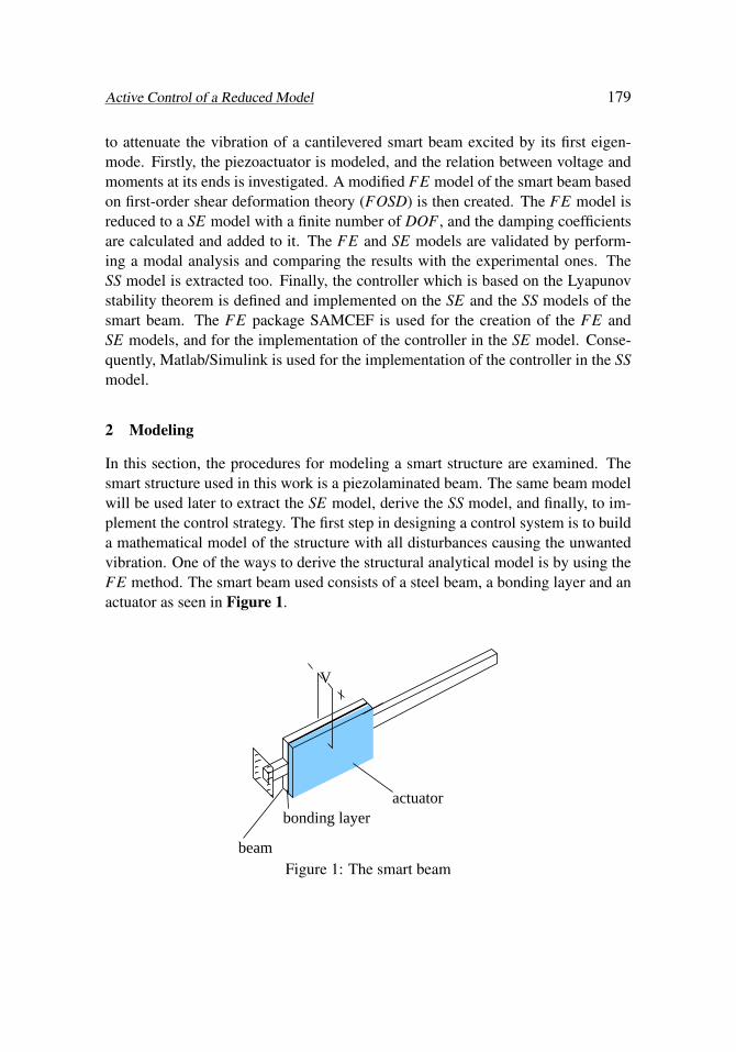
In this section, the procedures for modeling a smart structure are examined. Thesmart structure used in this work is a piezolaminated beam. The same beam modelwill be used later to extract the SE model, derive the SS model, and finally, to im-plement the control strategy. The first step in designing a control system is to builda mathematical model of the structure with all disturbances causing the unwantedvibration. One of the ways to derive the structural analytical model is by using theFE method. The smart beam used consists of a steel beam, a bonding layer and anactuator as seen in Figure 1.

actuator

V

beam

bonding layer

Figure 1: The smart beam


2.1 Actuator modeling

Using an actuator implies implementing an appropriate electric voltage to controlthe vibration of the smart structure (converse piezoelectric effect). Many FE pack-ages do not offer elements with electrical DOF . Consequently, the voltage appliedby the actuator can be represented by two equal moments with opposite directionsconcentrated at both ends [Crawley and Anderson (1990)]. The relation betweenactuator moments and actuator voltage can be investigated, so that the momentswill then act as the controlling parameters on the smart structure Figure 2.

elastic material

V

−−>

piezoceramic material

equivalent moment pair Mp

Figure 2: The induced stresses from a piezoceramic actuator

By considering the schematic layout of the middle portion of the smart beam (Figure 3),if a voltage V is applied across the piezoelectric actuator, assuming one-dimensionaldeformation, the piezo-electric strain εp of the piezo is:

εp =d31

tp·V (1)

where d31 is the electric charge constant and tp is the thickness of the piezoactuator.

na beam

actuator

adhesive2

3t

tt1

b

Z

Mp

zz

yMp

x

Figure 3: A schematic layout of the composite beam


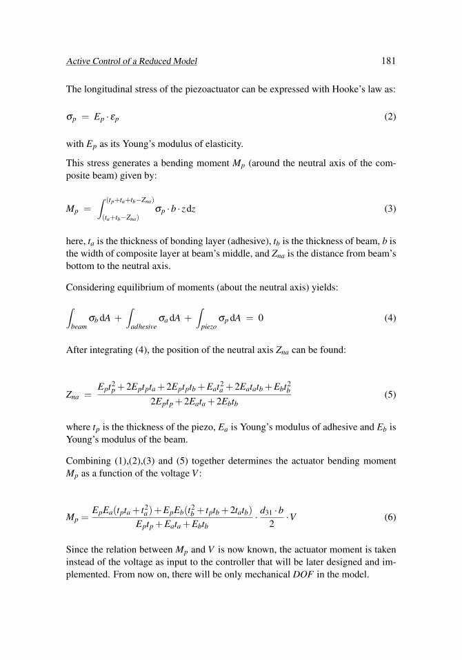
The longitudinal stress of the piezoactuator can be expressed with Hooke’s law as:

σp = Ep · εp (2)

with Ep as its Young’s modulus of elasticity.

This stress generates a bending moment Mp (around the neutral axis of the com-posite beam) given by:

Mp =∫ (tp+ta+tb−Zna)

(ta+tb−Zna)σp ·b · zdz (3)

here, ta is the thickness of bonding layer (adhesive), tb is the thickness of beam, b isthe width of composite layer at beam’s middle, and Zna is the distance from beam’sbottom to the neutral axis.

Considering equilibrium of moments (about the neutral axis) yields:

∫beam

σb dA +∫

adhesiveσa dA +

∫piezo

σp dA = 0 (4)

After integrating (4), the position of the neutral axis Zna can be found:

Zna =Ept2

p +2Eptpta +2Eptptb +Eat2a +2Eatatb +Ebt2

b

2Eptp +2Eata +2Ebtb(5)

where tp is the thickness of the piezo, Ea is Young’s modulus of adhesive and Eb isYoung’s modulus of the beam.

Combining (1),(2),(3) and (5) together determines the actuator bending momentMp as a function of the voltage V :

Mp =EpEa(tpta + t2

a)+EpEb(t2b + tptb +2tatb)

Eptp +Eata +Ebtb· d31 ·b

2·V (6)

Since the relation between Mp and V is now known, the actuator moment is takeninstead of the voltage as input to the controller that will be later designed and im-plemented. From now on, there will be only mechanical DOF in the model.


2.2 FE modeling

The resultant FE model of the smart beam must be faithfully representative in orderto use it for further applications like control analysis. To find the best FE model,the optimal element type and size must be selected. Thus, a modal analysis of thereal beam is experimentally performed and results of the natural frequencies arecompared with those from the FE model where different element types are used. Adetailed geometry of the smart beam is shown in Figure 4, and the material prop-erties and thickness of each part are represented in Table 1.

5layercomposite

10

5

10

10 75 130

Figure 4: A detailed geometry of the smart beam [dimensions in mm]

Table 1: Parameters of the components of the smart beam

Beam Bonding ActuatorMaterial steel epoxy resin PIC151Thickness [mm] 0.5 0.036 0.25Density [kg/m3] 7900 1180 7800Young’s mod. [MPa] 210000 3546 66667

The smart beam is created as a unique structure but modeled as a composite shellwith three layers. This means, all the three components of the model, i.e. beam,bonding layer and actuator are bonded together without any relative slip among thecontact surfaces. Consequently, each layer has its own mechanical properties. Tovalidate the choice of the FE type used (a composite shell element with 8 nodesbased on the FOSD), a modal analysis of the FE model is done and the first twoeigenfrequencies are read and compared to those from the experiment. This is seenin Table 2. As a boundary condition, the far left edge of the smart beam is clamped.

Concerning the optimal FE size to be used, it’s well known that reducing the FEsize will improve the solution accuracy. However, especially in the case of large


Table 2: Validation of element-type based on the modal analysis

FE model Experiment1st eigenfrequency [Hz] 13.81 13.262nd eigenfrequency [Hz] 42.67 41.14

complex structures, the use of excessively fine elements in the FE model may re-sult in unmanageable computations that exceed the memory capabilities of existingcomputers [Ko and Olona (1987)]. From Table 3, it is seen that using an element

Table 3: Effect of element size on the eigenfrequency

FE size [mm] 1st eigenfreq. [Hz] 2nd eigenfreq. [Hz]0.25 13.80 42.660.5 13.81 42.661.0 13.81 42.672.5 13.83 42.715 13.89 42.8110 14.09 43.21

size less than 1 mm does not make any significant change on the values of the 1stand 2nd eigenfrequencies of the smart beam. This means, it can be regarded as theoptimal value for the element size in the FE modeling.

Before this subsection is closed, it may be argued that the damped frequency fromexperimental modal analysis of the real model was compared to the undamped fre-quency of the FE model, where the damping coefficients are not yet calculated.This is true, but it does not have a big influence on the solution since the relationbetween the damped and the undamped frequencies in terms of the damping ratioξ is

ωdamped = ωundamped√

1−ξ 2 (7)

Thus, a direct comparison between both frequencies can be made since ξ � 1.


2.3 SE modeling

A super element, also termed substructure, is a complex element that includes anumber of finite elements used in a structural modeling. The main virtue of thistechnique is the ability to perform the analysis of a complete structure by using theresults of prior analysis of different regions comprising the whole structure [Gha-reeb and Weichert (2009)]. The application of the SE technique goes back to theearly 1960s when it has been used by aerospace engineers to break down the struc-ture of an airplane into simpler first-level substructures for enhancing the com-putaional efficiency [Fan, Tang, and Chow (2004)].The basic concept of substructuring is that all DOF , which are considered uselessfor the final solution, are condensed and the rest is retained. This means, the DOFof the whole system correspond to the retained nodes plus a number of internaldeformation modes (dynamic analysis problems).To construct a SE, or in other words to remove the unwanted nodes and DOF fromthe substructure, the method of "component mode synthesis" is used [Craig andBampton (1968)], and a linear SE is created. According to this method, the DOFof each substructure are classified into:

1. Boundary DOF shared by several structures

2. Internal DOF belonging only to the considered substructure

The behaviour of each substructure is described by the combination of two types ofcomponent modes:

1. The constraint modes (static deformed shape) which are determined by as-signing a unit displacement to each boundary DOF , while all other bound-aries DOF are being fixed

2. The normal vibration modes (dynamic deformed shape) that correspond tothe vibration modes obtained by clamping the structure at its boundary

It is then assumed that the behaviour of the substructure in the global system can berepresented by superimposing the constrained modes and a small number of nor-mal vibration modes. Taking an infinite number of modes would not help and doesnot make sense since only a few number of modes has a physical meaning [Hughes(1987)]. Hence, by retaining only the low-frequency vibration modes, the substruc-ture’s dynamically deformed shape can be represented with sufficient accuracy.

Starting from the FE model of the previous subsection, a SE model with a limitednumber of DOF will be created.


Firstly, the master or retained nodes must be selected. These correspond to thenodes where a boundary condition or a load is applied. The rest of the nodes willbe considered as slave or condensed nodes. In the FE model, 5 nodes are consid-ered as retained nodes (Figure 5).

1 4 52 3

Figure 5: The retained nodes of the SE

This means:

- Node 1 is used to introduce a boundary condition (clamping constraint).

- Node 2 is used to introduce a load (actuator moment).

- Node 3 is used to introduce a load (actuator moment).

- Node 4 is used to measure the displacement (distance sensor).

- Node 5 is used to measure the tip displacement (distance sensor).

Secondly, 10 modes, which correspond to 97% of the modal effective mass, areselected. The percentage of modal effective mass for each mode is usually foundinside the input file created by any FE software.To check the validity of the SE created, it has to be compared to the FE modelwhich was already validated before. Abstractly said, the reduced model must havethe same characteristics as the original model, except that the number of nodes isreduced, as well as the number of DOF . The eigenfrequencies of the first 2 modesresulting from each model are depicted in Table 4.

Table 4: Eigenfrequencies of the first two modes

Mode SE model [Hz] FE model [Hz] Experiment [Hz]1 14.249 13.811 13.262 43.414 42.673 41.14

The physical properties of each model are shown in Table 5. It is clear that both


models deliver almost the same value of the eigenfrequency for the first two modes.Since the excitation of the beam by its first eigenmode is concerned, furhter read-ings are not necessary. Compared to the FE model, the SE model has few numberof DOF and a very small number of nodes. It consists of a single element andhas the advantage that the simulation time becomes short and the controllers areimplemented on the SE model itself.

Table 5: Characteristics of the FE and SE models

FE model SE modelElement size [mm] 3.07Number of elements 2575 1Number of nodes 8206 5Number of DOF 16860 40

3 Damping Characteristics

Damping of structures has historically been of great importance in nearly all branchesof engineering endeavors. Mechanical and structural systems rely on various damp-ing mechanisms to dissipate energy during undesirable vibratory motions [Taylorand Nayfeh (1997)]. Damping parameters, which are also of significant importancein determining the dynamic response of structures, cannot be deduced deterministi-cally from other structural properties or even predicted by using the FE technique.For this reason, recourse must be made to data from experiments conducted oncompleted structures of similar characteristics. Such data is scarce in general, butthey are very valuable for studying the phenomenon and modeling of damping[Butterworth, Lee, and Davidson (2004)]. In fact, there are many non-linear damp-ing models available [Puthanpurayil, Dhakal, and Carr (2011)], but in this work thedamping is assumed to be viscous and frequency dependent for the sake of conve-nience and simplicity [Alipour and Zareian (2008)].With this linear approach, which was initially introduced by Rayleigh [Rayleigh(1877)], it is supposed that the damping matrix is in a linear combination of themass and stiffness matrices. Although this idea was suggested for mathematicalconvenience only, it allows the damping matrix to be diagonalized simultaneouslywith the mass and stiffness matrices, preserving the simplicity of uncoupled, realnormal modes as in the undamped case [Adhikari and Woodhouse (2001)]. The


relation is:

C = α M + β K (8)

where α and β are real scalars that must be determined.

The main advantage of this formulation is that the damping matrix will be a di-agonal matrix. The damping ratio ξ is related to the scalars α and β through therelation [Ghareeb and Schmidt (2012)]:

ξi =α

2 ωi+ β

ωi

2(9)

with ω as the eigenfrequency and the subscript i the mode number.

Here, two values for the eigenfrequency ωi with the corresponding values of ξi areneeded to find out the scalars α and β and thus to compute the damping matrix C.Two methods are used to find these damping characteristics. These are the methodof Chowdhury and Dasgupta [Chowdhury and Dasgupta (2003)], and the method ofdamping from normalised spectra, also known as the half-power bandwidth method[Butterworth, Lee, and Davidson (2004)],[Ewins (1984)]. Results from both meth-ods are represented in Table 6.

Table 6: Results of α and β from both methods

Chowdhury Half-power bandwidthα 0.02577 0.02955β 9.918×10−6 9.770×10−6

It can be noticed that both methods have shown that the damping is mass propor-tional, since α � β in both techniques. In this work, the average values of bothmethods are used, and the damping characteristics are added to the SE model andto the SS representation that will be derived in the next section.

4 State-Space Representation

4.1 Basics of the state-space representation

Beside the SE model, the SS representation is used as a second approach to im-plement the controller. The basic idea of this procedure is to describe a system of


equations in terms of n first-order differential equations. Hence, the use of vector-matrix notation greatly simplifies the mathematical representation of the system ofequations. On the other hand, the increase in the number of state variables, thenumber of inputs, or the number of outputs does not increase the complexity ofthese equations [Ogata (2002)]. This approach is used here in order to validate orcompare the results of the SE model.The state equations have the form:

x = A x + B uy = C x

(10)

and the size of the matrices A, B and C depends on the number of states, inputsand outputs of the system. Upon specifying the type and position of the input andoutput vectors, a FORTRAN code is used to create the SS model of the smart beam.This model is then integrated in Matlab/SIMULINK to give the dynamic responseof the modelled structure under one or several inputs and outputs.

4.2 Creation and validation of the SS equations for the case of a smart beam

The objective now is to create the SS representation of the smart structure investi-gated in this work, and to validate it by carrying out a simple simulation, so that theresults can be compared to those from the FE model. At the beginning, the inputsand outputs of the system must be specified. Referring to Figure 5, a sensor isplaced at Node 5 to measure the tip displacement, and the input will be a harmonicforce at the same node. Thus, the smart beam will be excited by its first eigenmode.The force F has the form:

F = c sin(ω1 t); with c as a constant (amplitude) (11)

Now, there is a single input and a single output. Since Node 1 is clamped, thenumber of states is defined as:

2p = 30 + 10 − 6 = 34 (12)

There are 30 DOF in the system, in addition to 10 vibration modes. Concerningthe dimensions of the matrices A, B, C:

dim(A) = 34×34dim(B) = 34×1dim(C) = 1×34

(13)

The SS representation of this smart beam is shown in Figure 6. The simulation iscarried out for 40 seconds while the load is kept active for the first 20 seconds. The


resulting curve in Figure 7 shows that both models had the same value of tip dis-placement throughout the simulation time. This gives more reliance to the results.However, both models will be used in the coming section for the implementationof the controller.

Tip displacement

Fy = Cxx’ = Ax + Bu

Figure 6: The SS model of the smart beam

0 5 10 15 20 25 30 35 40−0.04

−0.03

−0.02

−0.01

0.00

0.01

0.02

0.03

0.04Free vibration

Time [s]

Forced vibration

Tip

dis

plac

emen

t [m

]

SS model SE model

Figure 7: Free and forced vibration of the smart beam

5 Controller Design

5.1 Lyapunov Stability Theorem Controller

Although there is no general procedure for constructing a Lyapunov function, yetany function can be considered as a candidate if it meets some requirements, i.e.,positive definite, equal to zero at the equilibrium state and with its derivative lessor equal to zero [Khalil (1996)],[Bacciotti and Rosier (2005)]. Now, the energy


equation of a thin Bernoulli-Euler beam which is modelled as a single FE in a one-dimensional system with length h and left point coordinate xi, is considered as aLyapunov function candidate (Figure 8).

M (x ,t)

X, u

Y, v

h

z i

ix

F (x +h,t)s s F (x ,t)i i

M (x +h,t)z i

Figure 8: Section of the smart beam where the piezoelement is located

According to [Gorain and Bose (1999)], the total energy equation of a beam withoutany external forces or moments is:

U =12

∫ xi+h

xi

[ρA(

∂v∂ t

)2+ EI

(∂ 2v∂x2

)2]

dx (14)

where h is the length of the beam section, u and v are the displacements in longitu-dinal and transverse directions, E and ρ are the elastic modulus and density of thebeam.According to Figure 8, Mz is the actuator bending moment, Fs is the shear forceon the beam, and Iz is the second moment of inertia of its cross-section about the(bending) z-axis.

The above function is locally positive definite, continuously differentiable and equalto zero at the equilibrium state. Yet, to consider it as a Lyapunov function, thederivative of this function must be smaller or less than zero as well.Differentiating (14) in time leads to:

U =∫ xi+h

xi

[ρA

∂v∂ t

∂ 2v∂ t2 + EI

∂ 2v∂x2

∂

∂ t

(∂ 2v∂x2

)]dx (15)


Referring to the relationships for a vibrating beam, which are summarized in anyreference about beams like [Petyt (2003)], it reveals that:

ρA∂ 2v∂ t2 + EI

∂ 4v∂x4 = 0

Mz = EI∂ 2v∂x2

Fs = −EI∂ 3v∂x3

(16)

Substituting the derived equations for the bending moment Mz, shear force Fs, andassuming no shear after that, the first derivative yields:

U = Mz

[∂

∂ t

(∂v∂x

)]xi+h

xi= Mz

(v′xi+h − v′xi

)(17)

where v′xi is a rotational velocity at node xi.To ensure that (17) is always smaller or equal to zero, Mz, the actuator moment, canhave the value:

Mz = − k(

v′xi+h − v′xi

)(18)

with k as a positive constant, sometimes called "the proportionality factor". Varyingk has a significant effect on the response. Theoretically, the system is stable for anypositive value. Nevertheless, larger values of k tend to "overcontrol the structure"since the moment will have a magnitude larger than that required. Consequently,if k is very small, the added moments will be insufficient and this will reduce thedamping ratio. Therefore, a trial-and-error procedure is required to select the bestvalue and customize the control to the application [Newman (1992)].

Substituting (18) in (17) yields:

U = − k(

v′xi+h− v′xi

)2≤ 0 (19)

and thus, all the requirements to have a Lyapunov function are met. Therefore, (18)can be used as the controller for the smart beam.To implement this equation on the smart beam, the moments at node 2 and node 3,which are equal in magnitude but with opposite directions, are calculated as func-tions of the rotational velocites at both nodes [Ghareeb and Schmidt (2012)]. Theyhave the form:

M2y = −k (v2y − v3y)M3y = −k (v3y − v2y)

(20)


From the above equations, it is clear that the controller is in fact a connectionbetween the DOF of the nodes composing the SE. To do that in SAMCEF, thenonlinear forces element (FNLI) is used. This element allows the introduction ofa list of n general linear or nonlinear internal forces as a function of list of n DOFand their derivatives. The control strategy is defined directly inside the input filewithout the use of any external programming language, and this is one of the meritsof the SE technique.Coming back to the control law of (20), the controller is stable for any positivevalue of the constant k. At the beginning, three different values of k are taken, andthe results are depicted in Figure 9.

20 22 24 26 28 30 32 34 36 38 40−0.03

−0.02

−0.01

0

0.01

0.02

0.03

Time [s]

Tip

dis

plac

emen

t [m

]

No control Control, k=1 Control, k=5 Control, k=10

Figure 9: The Lyapunov stability theorem controller for different values of k (SEmodel)

Moreover, the choice of k has an influence on the amplitude of the resonance at thenatural frequency of the structure, which is seen in Figure 10. Now, the optimalvalue of the constant k must be found. Since the design of optimal controllersis not the task of this work, the method of trial-and-error is used to find out thisoptimal value. Best results are got for k = 30, and the corresponding curve of tipdisplacement vs. time of the smart beam is illustrated in Figure 11. In the FFTspectrum diagram (Figure 12), the effect of the controller on the amplitude of theresonance at the natural frequency is shown as well.

As stated before, the SS representation of the smart beam is derived in order tovalidate the results from the SE model. To do that, the inputs and the outputs are


10 11 12 13 14 15 16 17 18 19 200

0.01

0.02

0.03

0.04

0.05

0.06

Frequency [Hz]

Mag

nitu

de [

mm

]

No control Control, k=1 Control, k=5 Control, k=10

Figure 10: The FFT spectrum of the smart beam for different values of k (SE model)

20 22 24 26 28 30 32 34 36 38 40−0.03

−0.02

−0.01

0

0.01

0.02

0.03

Time [s]

Tip

dis

plac

emen

t [m

]

No control Control with k=30

Figure 11: The Lyapunov stability theorem controller for k = 30 (SE model)

designated in order to find out the matrices A, B and C of (10). To implement thecontroller in the SS model, two steps are performed. In step one, the only input tothe system is the forced excitation until the magnitude of vibration does not changeanymore, i.e., up to t = 20s, and the output consists of the tip displacement, as


0 5 10 15 20 250

0.01

0.02

0.03

0.04

0.05

0.06

0.07

Frequency [Hz]

Am

plitu

de [

mm

]

No control Control with k=30

Figure 12: The FFT spectrum of the smart beam using Lyapunov stability controller(SE model)

well as the state vectors exactly at t = 20s. The diagram is shown in Figure 13.

3

vTip displacement

v0

0y = Cxx’ = Ax + Bu 2

Figure 13: The SS model of the smart beam with controller (step 1)

These state vectors are then fed in as initial conditions in the second step. Thistime, the input comprises both actuator moments at both ends of the actuator, andthe output embraces the tip displacement at node 5, and the velocities at the node 2and node 3.The steps mentioned above could be also summarized in one step, but in this case atimer must be inserted in the model to deactivate the exciting force when vibrationsbecome stable at t = 20s. The SS representation of the smart beam in the secondstep is shown in Figure 14.A comparison of the results from the SE model and the SS model is shown in


3

Tip displacement

M kv

vx’ = Ax + Buy = Cx

0

M

2

2

3

Figure 14: The SS model of the smart beam with controller (step 2)

Figure 15 and Figure 16 where the time region between 20 and 22 s is magnified.It can be seen that both models yielded the same results. Nevertheless, much more

20 21 22 23 24 25 26 27 28 29 30

−0.03

−0.02

−0.01

0.00

0.01

0.02

0.03

Time [s]

Tip

dis

plac

emen

t [m

]

SS model SE model

Figure 15: Tip displacement vs. time using SE and SS models

time was needed to carry out the simulation in the SS model (about 35 minutes),while in the SE model, less time (only 3 minutes) was needed. This could be due tothe fact that in the SE model a fixed time-step can be assigned (here 0.01 s), whilein the SS representation the time-step was automatically set. Moreover, the stressesand energy curves, could be requested in addition to the force vectors along theSE model. This is one of the advantages of the SE technique in comparison to theSS representation which is more practical and in which the controller can be easilyimplemented [Ghareeb and Schmidt (2012)].


20 20.2 20.4 20.6 20.8 21 21.2 21.4 21.6 21.8 22

−0.03

−0.02

−0.01

0.0

0.01

0.02

0.03

Time [s]

Tip

dis

plac

emen

t [m

]

SS model SE model

Figure 16: Tip displacement vs. time in a zoomed region of Figure 15

6 Summary

In this work, a linear controller based on the Lyapunov stability theorem was de-signed and implemented on a reduced model of a smart structure. The super el-ement technique was used to create this reduced model starting from the finiteelement model. A state-space representation of the same model was extracted aswell. The controller was implemented on this model too, and the results from bothmodels were compared.

References

Adhikari, S.; Woodhouse, J. (2001): Identification of damping: Part 1, viscousdamping. Journal of Sound and Vibration, vol. 243, pp. 43–61.

Alipour, A.; Zareian, F. (2008): Study rayleigh damping in structures; uncertain-ties and treatments. In the 14th world conference on earthquake engineering.

Bacciotti, A.; Rosier, L. (2005): Liapunov Functions and Stability in ControlTheory. Springer.

Bailey, T. (1984): Distributed-parameter vibration control of a cantilever beamusing a distributed-parameter actuator. Master’s thesis, Massachusetts Institute of


Technology (MIT), 1984.

Bailey, T.; Hubbard, J. J. (1985): Distributed piezoelectric-polymer active vi-bration control of a cantilever beam. AIAA Journal of Guidance and Control, vol.6, No. 5, pp. 605–611.

Benjeddou, A. (2000): Advances in a piezoelectric finite element modeling ofadaptive structural elements: a survey. Computers and Structures, vol. 76, pp.347–363.

Butterworth, J.; Lee, J.; Davidson, B. (2004): Experimental determination ofmodal damping from full scale testing. In 13th world conference on earthquakeengineering.

Chowdhury, I.; Dasgupta, S. (2003): Computation of rayleigh damping coeffi-cients for large systems. The electronic Journal of geotechnical engineering, vol.8.

Ciaurriz, P. (2010): Active vibration control of a flexible beam by using a co-simulation of adams/flex and matlab/simulink. Master’s thesis, RWTH AachenUniversity of Technology, 2010.

Craig, R. R.; Bampton, M. (1968): Coupling of substructures for dynamicanalyses. AIAA Journal, vol. 6, pp. 1313–1319.

Crawley, E.; Anderson, E. (1990): Detailed models of piezoelectric actuation ofbeams. Journal of Intelligent Material Systems and Structures, vol. 1, pp. 4–24.

Crawley, E. F.; de Luis, J. (1987): Use of piezoelectric actuators as elements ofintelligent structures. AIAA Journal, vol. 25, No. 10, pp. 1373–1385.

Ewins, D. J. (1984): Modal Testing. John Wiley & Sons Inc.

Fan, J. P.; Tang, C. Y.; Chow, C. L. (2004): A multilevel superelement techniquefor damage analysis. International Journal of Damage Mechanics, vol. 13, pp.187–199.

Fanson, J.; Caughey, T. (1990): Positive position feedback control for largespace structures. AIAA Journal, vol. 28, pp. 717–724.

Ghareeb, N.; Radovcic, Y. (2009): Fatigue analysis of wind turbines. DEWImagasin, vol. 35, pp. 12–16.

Ghareeb, N.; Schmidt, R. (2012): Modeling and active vibration control of asmart structure. Proceedings of the 9th international Conference on Informatics inControl, Automation and Robotics (ICINCO 2012), Rome, Italy, vol. 1, No. 86, pp.142–147.


Ghareeb, N.; Weichert, D. (2009): Combined multi-body-system and finiteelement analysis of a complex mechanism. Proceedings of the 11th SAMCEFUser Conference, Paris.

Gorain, G. C.; Bose, S. K. (1999): Boundary stabilization of a hybrid euler-bernoulli beam. In Proc. Indian Acad. Sci. (Math. Sci.).

Hughes, P. C. (1987): Space structures vibration modes: How many exist? whichones are important? IEEE Control Systems Magazine, pp. 22–28.

Hwang, W.; Park, H. (1993): Finite element modeling of piezoelectric sensorsand actuators. AIAA Journal, vol. 31, No. 5, pp. 930–937.

Kapuria, S.; Yasin, M. (2010): Active vibration control of piezoelectric lami-nated beams with electroded actuators and sensors using an efficient finite elementinvolving an electric node. Smart Mater. Struct., vol. 19, pp. 1–15.

Khalil, H. (1996): Nonlinear Systems. Prentice Hall, Madison.

Ko, W.; Olona, T. (1987): Effect of element size on the solution accuraciesof finite-element heat transfer and thermal stress analysis of space shuttle orbiter.Memorandum 88292, NASA, 1987.

Lim, Y.; Varadan, V.; Varadan, V. (1997): Closed loop finite element modelingof active structural damping in the frequency domain. Smart Mater. Struct., vol. 6,pp. 161–168.

Mallock, A. (1905): A method of preventing vibration in certain classes ofsteamships. Trans. Inst. Naval Architects, vol. 47, pp. 227–230.

Manning, W.; Plummer, A.; Levesley, M. (2000): Vibration control of a flexiblebeam with integrated actuators and sensors. Smart Mater. Struct., vol. 9, pp. 932–939.

Newman, S. M. (1992): Active damping control of a flexible space structure usingpiezoelectric sensors and actuators. Master’s thesis, Naval Postgraduate School,1992.

Ogata, K. (2002): Modern Control Engineering. Prentice Hall.

Petyt, M. (2003): Introduction to Finite Element Vibration Analysis. CambridgeUniversity Press.

Piefort, V. (2001): Finite Element Modelling of Piezoelectric Active Structures.PhD thesis, Université Libre de Bruxelles, Belgium, 2001.

Puthanpurayil, A.; Dhakal, R.; Carr, A. (2011): Modelling of in-structuredamping: A review of the state-of-the-art. In Proceedings of the ninth pacificconference on earthquake engineering, Auckland, New Zealand.


Rayleigh, L. (1877): Theory of Sound. Dover Publications.

Taylor, T. W.; Nayfeh, A. H. (1997): Damping characteristics of laminated thickplates. Journal of Applied Mechanics, vol. 64, pp. 132–138.

Vang, A. (1944): Vibration dampening, 1944. Patent No. 2,361,071, USA.

Vepa, R. (2010): Dynamics of Smart Structures. John Wiley & Sons Ltd.

active control of a reduced model of a smart structure · active control of a reduced model of a...

Documents