Active Data Structures and Applications to Dynamic and Kinetic

Algorithms

Kanat Tangwongsan (ktangwon@cs.cmu.edu)

Advisor: Guy Blelloch (guyb@cs.cmu.edu)

May 5, 2006

Abstract

We propose and study a novel data-structuring paradigm, called active data structures. Likea time machine, active data structures allow changes to occur not only in the present butat any point in time—including the past. Unlike most time machines, where changes to thepast are incorporated and propagated automatically by magic, active data structures system-atically communicate with the affected parties, prompting them to take appropriate actions.We demonstrate an efficient maintenance of three active data structures: (monotone) priorityqueue, dictionary, and compare-and-swap.

These data structures, when paired with the self-adjusting computation framework, createnew possibilities in kinetic and dynamic algorithms engineering. Based on this interaction, wepresent three practical algorithms: a new algorithm for 3-d kinetic/dynamic convex hull, analgorithm for dynamic list-sorting, and an algorithm for dynamic single-source shortest-path(based on Dijkstra). Our 3-d kinetic convex hull is the first efficient kinetic 3-d convex hullalgorithm that supports dynamic changes simultaneously.

This thesis provides an implementation for selected active data structures and applications,whose performance is analyzed both theoretically and experimentally.

1 Introduction

Motion is truly ubiquitous in the physical world. Perhaps, equally ubiquitous are contexts inwhich critical need arises for computation to support motion effectively. The class of computationcapable of handling motion is often called kinetic algorithms (data structures). In the simplest form,kinetic algorithms maintain a combinatorial structure as its defining objects undergo a prescribedmotion. Over the past decades the algorithmic study on the subject has made significant theoreticaladvances for many problems, yet leaving many important basic problems open [Gui04]. However,only a small number of these algorithms are successfully implemented and used, mostly becausethe algorithms are highly intricate.

This thesis was initially motivated by an open problem in computational geometry—kinetic 3-dconvex hull—that we later made some progress on. By now, it is hard to overstate the importanceof maintaining the convex hull of a set of points. However, while much is known for d = 2 [BGH97,Gui04], the problem of maintaining the kinetic convex hull for dimension d ≥ 3 has remained open.For d = 3, the best known algorithm re-computes the convex hull entirely as need arises. Our

1

approach to solving the kinetic 3-d convex hull problem has centered on devising a general-purposetechnique for handling motion and other types of changes. We attempted to extend the self-adjusting computation framework [Aca05, ABB+05, ABBT06] to support motion (i.e. continuouschanges). This study poses two fundamental questions which we answer affirmatively in this thesis:

1. Is there a natural class of data structures that are closely related to the behaviors of incre-mental computation (or more generally, dynamic/kinetic algorithms) of which the design andanalysis of dynamic/kinetic algorithms can take advantage?

2. If these data structures exist, can they be integrated to self-adjusting computation to alleviatethe task of dynamic/kinetic algorithms engineering in a natural way?

We propose and study a novel data-structuring paradigm, called active data structures. Like atime machine, active data structures allow changes to occur not only in the present but at any pointin time—including the past. Unlike most time machines, where changes to the past are incorporatedand propagated automatically by magic, active data structures systematically communicate withthe affected, prompting them to take appropriate actions. We demonstrate an efficient maintenanceof three active data structures: (monotone) priority queue, dictionary, and compare-and-swap.

Given a time machine and an ordinary algorithm, it is not hard to simulate a dynamic/kineticalgorithm. An ordinary algorithm refers to long-familiar algorithms that cannot account for changesthat take place on the fly. As an example, consider constructing a dynamic shortest-path algorithm.First, start the time machine. Then, run Dijkstra to the given graph G. This computes the shortest-path for the graph G. To update the graph G, tell the time machine to revert to the beginning oftime, update the graph, and tell the time machine to return to the present. The resulting shortest-path now corresponds to the new graph, as desired. Even though no time machine are publiclyaccessible, self-adjusting computation somewhat mimics that behavior.

Active data structures can naturally interact with self-adjusting computation. This thesis pro-vides an implementation for selected active data structures and applications. We show that activedata structures can help simplify and improve many dynamic algorithms. Section 4 illustrates asimple use of active data structures to the dynamic list-sorting problem.

In Section 5, we describe a new practical algorithm for maintaining the kinetic 3-d convex hullbased on active data structures. This algorithm greatly improves on the naive method. We verifythe effective of our approach both theoretically and empirically. We describe an algorithm fordynamic shortest-path in Section 6. We conclude this paper by discussing about work in progressand pointing out some directions for future work.

2 History and Background

The ability to efficiently maintain the output of a computation as the input undergoes changeshas been proven crucial in a countless number of real-world applications. Dynamic changes arediscrete changes involving insertions and deletions of objects in the input. Algorithms that handledynamic changes are called dynamic algorithms. Over the past decades, the algorithms communityhas extensively studied this class of algorithms and made significant theoretical advances. De-spite tremendous efforts, many of these algorithms are never successfully implemented, as they arecomplicated, making the task of implementing and debugging them highly strenuous.

2

Over the same period of time, the programming languages community has put efforts into de-veloping tools to cope with and combat the implementation challenges of dynamic algorithms. Amajor line of research has focused on devising techniques for transforming static programs to theirdynamic counterparts. Many of these techniques build on the idea of incremental computation.Early work on incremental computation [DRT81, PT89, ABH02, Car02] has shown that the tech-nique can deliver competitive performance to handcraft algorithms and are applicable to a broadrange of problems.

2.1 Self-Adjusting Computation

Self-adjusting computation is an attempt to bring together techniques in the algorithms commu-nity and the programming languages community. The approach provides a technique for semi-automatically transforming static programs to programs that can adjust to changes to their inputs(and internal states). The transformation in the self-adjusting computation framework does notgenerate a dynamic-algorithm description for the given static algorithm. Instead, think of self-adjusting computation as a special machine that learns about actions that a program (an algorithm)performs and is capable of intelligently re-executing parts of the program as changes occur. Weterm the process of smart re-execution “change-propagation”. A smart re-execution, as opposeda blind re-execution, selectively re-executes parts of computations as needed and reuses resultsof computations whenever permissible. Theoretical evidence suggests that smart re-execution ishighly effective for many classes of problems.

Self-adjusting computation relies on two key ideas: dynamic dependence graph (or DDG) andmemoization [Aca05, ABH02]. During the execution of a self-adjusting program, the run-timesystem builds a DDG, which records the relationship between computation and data. After a self-adjusting program completes its execution, the user can change any computation data (e.g., theinputs) and update the output by performing a change propagation. This change-and-propagatestep can be repeated. The change-propagation algorithm updates the computation by mimickinga from-scratch execution.

We state some definitions and certain properties of self-adjusting programs. A detailed treat-ment of the subject can be found in [Aca05, ABB+05, ABBT06, ABH+04].

Definition 1 Let I the set of possible start states (inputs). A class of input changes is a relation∆ ⊆ I × I. The modification from I to I ′ is said to conform the class of input change ∆ if andonly if (I, I ′) ∈ ∆. For output-sensitive algorithms, ∆ can be parameterized according to the outputchange.

Definition 2 A trace model consists of a set of possible traces T . For a set of algorithms A,a trace generator is the function T : A × I → T , and a trace distance is the function δtr (·, ·) :T × T → Z

+.

Let Eφ[X] denote the expectation of the random variable X with respect to the probability-density function φ, we define expected-case stability as follows.

Definition 3 (Expected-Case Stability) For a trace model, let P be a randomized program,let ∆n a class of input changes parametrized n, possibly the size of the input, and let φ(·) be a

3

probability-density function on bit strings 0, 1∗. For all n ∈ N, define

d(n) = max(I,I′)∈∆n

Eφ[δtr

(

tr(P, I), tr(P, I ′))

].

We say that P is expected S-stable for ∆ and φ if d(·) ∈ S.

Note that expected O(f(·)) stable, Ω(f(·)) stable, and Θ(f(·)) are all valid uses of the stabilitynotation. Worst-case stability is defined by dropping the expectation from the definition.

We define monotonicity of a program as in Acar et al. [ABH+04] and state the following theo-rems, which are useful in the sequel.

Theorem 4 (Stability Theorem [ABH+04]) If an algorithm is O(f(n))-stable for a class ofinput changes ∆, then each operation will take at most O(f(n) log n).

However, if the discrepancy set has a bounded size, then each operation can be performed inO(f(n)).

Theorem 5 (Triangle Inequality for Change Propagation) Let P be a monotone programwith respect to the class of changes ∆1 and ∆2. Suppose that P is O(f(n)) and O(g(n)) stablefor ∆1 and ∆2, respectively, for some measure n. P is also monotone with respect to the class ofchanges (∆1 ∆2) obtained by composing ∆1 and ∆2, then P is O(f(n)+g(n)) stable for ∆1 o ∆2.

A proof of this theorem is supplied in the appendix.

3 Active Data Structures

We introduce a new data structuring paradigm, called active data structures. Akin to the retroactivedata structures [DIL04], active data structures allow the data-structure operations to take placenot only in the present but also in the past. When an operation is performed, an active datastructure, in addition to fixing the internal states, identifies which other operations take on newresulting values and notifies them to adjust to the changes. This capability has an importantsoftware-engineering benefit: composibility.

Consider a database for bank accounts at a financial company. Suppose that, at 12pm, we dis-cover that an important transaction performed earlier at 9am was erroneous, and we need to correctit. Most traditional systems would need to rollback the transactions to 9am, where we then correctthe record and recommit subsequent transactions. Using a retroactive data structure [DIL04], onewould, in one-step, magically tell the data structure to correct the operation performed at 9am andrejoice. However, it is often inadequate to make corrections only internally to the data structure.In this example, suppose further that a banker performed a query at 10am, whose result is used inan investment plan recorded to the database at 11am. It is critical to notify the person performingthe query at 10am to consider the new value and update the plan.

Comparison to Persistent Data Structures. While persistent data structures and activedata structures both consider the notion of time, they are inherently different—both in terms of

4

Time6AM 9AM 12PM

...

Transactions

Err

oneous T

ransacti

on

Bob

Pla

nnin

g

Deci

sion

Dis

cover

the E

rror

Figure 1: The ability to change the past can be important. Many real-world applications alsorequire composibility.

their functionalities and the underlying ideas. A persistent data structure is characterized by theability to access any past versions of the data structure. In terms of changes, the simplest form ofpersistency, called partial persistency, allows changes only in the present and queries for any pastversions. A fully persistent data structure, although allowing changes to occur in the past, does notpropagate the effects of the changes to the present. Instead, it creates a new branch in the versiontree, as illustrated in Figure 2.

Time/Versions

An action in the past causes

the version tree to branches off

Figure 2: Changes to the past in a fully persistent data structure.

Comparison to Retroactive Data Structures. Even though retroactive data structuresand active data structures appear highly related as they both allow changes to occur in the presentand in the past, they significantly differ. In a retroactive data structure, operations performed onthe data structure are reflected only internally. An outside party who retrieves some data fromthe data structure has no way of knowing that the data is outdated. This is illustrated by thebank-database example mentioned earlier. In an active data structure, the affected parties will becommunicated.

The Notion of Time and Maintaining a Virtual Time Line. In order for the notionof time to make sense, we assume a time line is somehow maintained so that each action can betimestamped with a unique time. In practice, a virtual time line can be maintained efficiently usingan order-maintenance data structure [DS87, BCD+02]. These order-maintenance data structurescan simulate a virtual time line in amortized O(1). In what follows, we assume a time line is theset of non-negative reals (R+ ∪ 0), and each time-stamp is a unique real number t ∈ R

+ ∪ 0.

5

3.1 Defining Active Data Structures

We introduce vocabularies for discussing about active data structures. For comparison, considera usual data structure D with operations operation1, operation2, operation3, . . . , operationk. Ina usual data structure, all operations are performed at the present time, altering the state of thedata structure and destroying the previous version. An active data structure enables performing(or undoing) the operations at any time. We define 3 meta-operations that characterize active datastructures as follows:

• The meta-operation perform(“operationi(·)”, t) will perform the operation operationi at thetime t. If operationi(·) returns a value ri, then the meta-operation returns the value ri.

• The meta-operation undo(t) causes an undo of the operation at the time t.

• The meta-operation update(t) informs the data structure to “synchronize” up to time t. Thisoperation will become more clear once it appears in context.

In addition, we assume the existence of a discrepancy set; this is maintained either by the datastructure itself or as a part of another framework (cf. self-adjusting computation). The discrepancyset is a list of entities (e.g., a data structure operation, human interaction) that need to take someactions, because the information the entity receives has changed since the last communication.In the banking example, an entity could be Bob, who needs to know that the information heobtained is now outdated. The idea of the discrepancy set is that, as soon as an entity is identify asdiscrepant, it is inserted to the set. The entries of the discrepancy set are removed and processedin an increasing order of time until the set becomes empty, at which point the data structure isfully synchronized with the current reality. In practice, the discrepancy set can be maintained in apriority queue.

3.2 Active Compare-and-Swap

We begin our discussion of active data structures by introducing a basic data structure, calledcompare-and-swap. Despite its fancy name, a compare-and-swap data structure is a plain-old datastructure commonly found in algorithms. Without the notion of time, the data structure has onlyone operation, touch, and maintains a boolean variable b, whose value is initially false. If thedata structure is touched, the variable b changes to true and remains true for the rest of the time.The touch operation returns the current status of b and subsequently updates the value of b.

This simple data structure appears extensively as a tiny component of bigger data structuresand algorithms. It is, for example, a part of the bit vector in many implementations of depth-firstsearch, indicating whether or not a node has been visited. The name compare-and-swap emergesfrom the actions it performs. In many applications, once b is set to true no more operation will beperformed on the corresponding object.

Similar to a regular compare-and-swap, an active compare-and-swap has only one operation,touch, which can be both performed and undone at an arbitrary time. We formally describe anactive compare-and-swap as follows. This description outlines the general characteristics of the datastructure; an efficient compare-and-swap will be discussed later. Let S be the set of times at whichthe data structure is touched. Initially S is an empty set. For the purpose of this presentation,

6

think of S as a global variable, which is updated as operations are performed on the data structure.Like any active data structures, an active compare-and-swap supports the following:

• Support for the meta-operation perform. The operation perform(“touch”, t)—performinga touch at time t—maintains the following invariants. The return value of the operation isfalse if and only if t < min S, with min ∅ = +∞. After the operation, the set S is augmentedto contain t. That is, S := S ∪ t.

• Support for the meta-operation undo. The operation undo(t)—undoes a touch at timet—updates the set S as S := S \ t.

• Support for the meta-operation update. The operation checks if the return value of thetouch operation at that time has changed. If the value is changed, it tells the discrepancyset that the person who retrieves this information is discrepant.

We point out that both of these operations may alter the return values of some other touch

operations. An active compare-and-swap data structure has to be able to identify these operationsand re-synchronize accordingly.

Efficient Compare-and-Swap. In the remaining of this section, we describe an efficientmaintenance of an active compare-and-swap data structure. For ease, we maintain the set S in abalanced search tree (e.g. red-black tree). Maintaining S as a combination of a priority queue and ahash table is an equally viable option and will yield the same asymptotic bounds. The needed basicset operations, including finding the minimum, can be trivially performed on a balanced binarysearch tree in O(log |S|).

As mentioned earlier, an operation can affect the return values of other operations. We observethat, in this particular data structure, an operation can affect at most 1 other operation. Performinga touch at the time t will cause a side-effect if and only if t < min S, in which case the return valueof the old minimum is altered. An undo of the operation at time t causes a side-effect if only if t isthe current minimum of S, in which case the return value of the second minimum of S is changed.We note that the number of active touch’s T is same as |S| throughout, and establish the followingtheorem.

Theorem 6 An active compare-and-swap can be maintained in O(log T ) for all operations, whereT is the number of active touch’s. We say that a touch operation is active if it has been performedand has not been undone.

3.3 Active Monotone Priority Queue

We consider the problem of maintaining an active monotone priority queue. The monotone assump-tion greatly simplifies the problem but suffices for many applications; at the end of this section, wediscuss problems with generalizing this to an unrestricted priority queue. Without loss of generality,we assume that the keys (a.k.a. priorities) are positive real numbers (R+) Informally, a monotonepriority queue disallows inserting a key smaller than latest minimum removed by the deleteminoperation. We precisely formulate the problem and formally state this assumption below.

7

Let DM be the set of times at which a deletemin occurs. Let INS be the set of ordered pairs ofthe form (k, t). Each entry (k, t) ∈ INS denotes the insertion point of the key k at the time t. Weassume for simplicity that no duplicate keys are inserted.

Definition 7 Let PQ(t) be the set containing all keys inserted on or before the time t that have notbeen removed by the deletemin operation. The set PQ(t) is a hypothetical snapshot of the priorityqueue at time t. Initially PQ(0) = ∅.

Definition 8 (Monotone Assumption) Let f(t) := minPQ(t). A priority queue is said to bemonotone if for all t1, t2 ∈ DM with t1 < t2, f(t1) < f(t2).

Our priority queue supports two operations: insert and deletemin. The problem of maintainingactive priority queue has the following characteristics:

• Support for the meta-operation perform. The operation perform(“insert(k)”, t)—performingan insertion of the key k at time t—causes the following changes: INS := INS∪ (k, t). Thisoperation returns nothing.

The operation perform(“deleteMin”, t) calculates the return value as min PQ(t) and altersDM to DM∪ t. We note that this description does not describe how to efficiently maintainsuch a structure.

• Support for the meta-operation undo. The operation undo(t) for an insert operationsimply removes the corresponding (∗, t) from INS. Similarly, the operation undo(t) for andeleteMin operation removes t from DM.

* * * * * * * *

Efficient Monotone Priority Queue. We give a solution to the problem of efficiently main-taining an active monotone priority queue. Our data structure maintains 2 balanced binary searchtrees (e.g. red-black, AVL tree): TDM and TINS, corresponding to the sets DM and INS, respectively.The tree TDM is naturally ordered by time. The other tree TINS is indexed by first the key thenthe the time. That is, (k1, t1) < (k2, t2) if and only if (k1 < k2) or ((k1 = k2) ∧ (t1 < t2)). Eachdeletemin—a node of TDM—is linked with a node of TINS whose key is the result of that deletemin.Each node of TINS is vice versa linked with its corresponding deletemin when applicable.

As an active data structure, our active priority queue is responsible for identifying the operationswhose return values are affected, in addition to maintaining the invariants stated earlier. Theproblem of identifying the affected operations are discussed later. We will now focus on the problemof the maintaining the aforementioned invariants:

• The operation perform(“insert(k)”, t) results in an insertion of the key (k, t) to the tree TINS.The undo operation for an insert is handled vice versa by removing the key (k, t) from thetree.

• The operation perform(“deletemin”, t) adds an entry t to the tree TDM, and its undo operationremoves t from TDM. The return value of perform(“deletemin”, t) is derived as follows.

8

Compute t− := maxt′ ∈ DM : t′ < t, with max ∅ = −∞. If t− = −∞, report the minimumkey in TINS. Otherwise, query TDM for the corresponding value the delete; call this valuek−. Make another query to TINS for k∗ := mink′ ∈ Keys(INS) : k′ > k−, where Keys(INS)contains all the keys existed in INS. Report k∗. It is trivial to fix the cross-links between thetwo trees.

* * * * * * * *

A Ray-shooting Game and Discrepancy Detection. We introduce a “ray-shooting” game,which illustrates the processing of finding the affected operations. Every sequence of operationsin a retroactive data structure can be visually represented as follows. Consider a two-dimensionaldiagram, whose horizontal axis represents time and vertical axis represents the keys of the elementsof interest. Recall that each key is a positive real number. An example of such diagram is shown inFigure 3 (left). Each horizontal line represents the lifespan of its corresponding key. It originateswhere the key is inserted and extends to the right either indefinitely if it is never removed bya deletemin or until it vanishes at the time when removed by a deletemin. Each vertical linerepresents a deletemin operation. It always originates from the horizontal axis and extends upwardup to the height of the key that the deletemin operation returns.

t

ke

ys

t

ke

ys

A

B

Figure 3: Visualizing an Active Priority Queue using Ray-shooting

The task of identifying the affected operations can thought of as two cases of ray shooting:rightward and upward. Inserting a key k at time t is equivalent to ray-shooting rightward fromthe point (t, k), as depicted in the point A in Figure 3 (right). We say that a line segment isoccupied if it meets with another line segment of a different orientation. Removing a key will“free” a vertical segment; such a segment is affected. A new return value for that deletemin canbe calculated by performing an upward ray-shooting as depicted at point B in Figure 3 (right).The two other operations can be handled similarly. With the monotonicity assumption, these ray-shooting operations can be efficiently performed on the two trees in O(log T ), where T is the totalnumber of active operations on the data structure. As before, an operation is active if it has beenperformed but not undone.

Theorem 9 An active monotone priority queue can be maintained in an amortized O(log T ) for

9

all operations, where T is the number of active operations.

We point out that an active full priority queue is much more involved, as it demands a point-location data structure. In particular, the trick that allows us to compute the current minimumwill not generalize, because it relies on the monotonicity assumption. We conclude the discussionof active priority queues by listing a number of applications that admit the monotone assumption.In Dijkstra, the distance of the nodes as maintained in a priority is monotone. The same is truefor Prim’s algorithm for computing a minimum spanning tree. A monotone priority queue can alsobe used to ensure that certain operations are performed in order. Two real-world applications thatillustrate such use are discussed in a subsequent section.

3.4 Active Dictionary

A dictionary data structure supports three basic operations: insert(key, data), lookup(key), anddelete(key). Let U be the universe of keys the dictionary supports. We assume that either U istotally ordered or there exists a universal hash function h : U → [m] for m ∈ N. This assumptionis realistic and allows an easy maintenance of an active dictionary.

Like other active data structures we discuss, an active dictionary has the same three operations—insert, lookup, and delete—wrapped in the meta-operations perform, undo, and update. In order tosupport these operations, an active dictionary maintains the following structures internally. Eachkey k ∈ U is associated with three sets: INS(k), DEL(k), QUERY(k). First, the set INS(k) keepstrack of all insert operations performed on the key k. Entries of this set take the form (t, d), wheret denotes the time and d is the data associated with that insertion. Second, the set DEL(k) containsthe times at which delete operations are performed on the key k. Finally, the set QUERY(k) recordsthe times at which queries to the key k take place. These sets can be trivially maintained for therequired data structure operations.

Efficient Active Dictionary. The problem of maintaining an active dictionary can be reducedto a simpler problem in the following manner. When an operation about a key k is received, the datastructure refers to the three sets—INS(k), DEL(k), and QUERY(k)—on which actions are performed.We note that it suffices to consider only these three sets to support any operations regarding thekey k. Because of our assumption about the universe of keys, locating the corresponding three setscan be easily accomplished by a hash table or a (balanced) binary search tree.

We now turn our focus to maintaining the three sets for each key and how they can be usedto support all dictionary operations. Therefore, when the context is clear, we drop the mention ofkey. Consider Figure 4. The sets INS and DEL combine to a set of intervals in which the key ispresent in the dictionary. Formally, let

d>(t) := t′ ∈ DEL : t′ > t

andIV := (α, inf d>(α)) : α ∈ TIME(INS) ,

where (α, β) denotes the open-interval from α to β (exclusive), and inf(·) is the infimum. We notethat at most one interval is unbounded, corresponding to an insertion which is never deleted. Alookup at time t finds the key (and its corresponding data) if and only t lies in one of the intervals

10

Intervals

DEL

INS

( ( () ) )Queries

Q

Figure 4: The sets INS and DEL combine to a set of intervals in which the key is present in thedictionary.

of IV. If a lookup at time t satisfies t ∈ (α, β) for (α, β) ∈ IV, then the lookup operation finds thekey, where the data is the data of the insertion at time α.

Let Tk be the number of operations on which the key k. The sets INS, DEL, and QUERY canbe trivially represented with balanced binary search trees, where needed operations take at mostO(log Tk) time.

Theorem 10 For a fixed key k, an active dictionary can be maintained in an amortized O(log Tk)for all operations, where Tk is the number of active operations on the key k. Let n the total numberof keys. Assume that a balanced binary search tree is used to locate the right triple of sets; then,every operation in the active dictionary runs in O(log n + log Tk).

4 Dynamic Heap Sort

We demonstrate how an active data structure can be used in conjunction with the self-adjusting li-brary to implement a dynamic algorithm. We consider a simple problem of maintaining a sorted list:Given a list L, the algorithm maintains sort(L) under possible changes to L—insertions/deletionsof elements. In the static scenario, this can be easily accomplished by a heap as in Algorithm 1.

Algorithm 1 Simple Heap Sort on a List L

1: PQ ← ∅2: foreach x ∈ L do PQ ← PQ ∪ x3: L′ ← nil

4: while PQ is not empty do5: x ← deleteMin(PQ)6: Append x to L′

7: end while

The Standard ML code in Figure 5 shows a dynamic (self-adjusting) heap sort, using an activepriority queue. The function feed inserts the list elements of L into the priority queue, and thefunction reel assembles a sorted list based on the deleteMin operation.

11

fun feed l =

l o→ (fn c ⇒(case c of

ML.NIL ⇒ ()

| ML.CONS(h, t) ⇒ t o→ (fn ct ⇒ liftFeed ([Box.indexOf h],ct) (fn t ⇒let val () = PQ.insert mpq h

in feed t

end))))

fun reel () =

(PQ.deleteMin mpq) o→ (fn vopt ⇒case vopt of

NONE ⇒ ML.write ML.NIL

| SOME(h) ⇒ liftReel ([Box.indexOf h])(fn () ⇒let val tail = C.modref(reel ())

in ML.write (ML.CONS(h, tail))

end))

Figure 5: Dynamic Heap Sort in Standard ML

5 Dynamic and Kinetic Convex Hull in 3-d

Figure 6: 3-d convex hull of a set of points

Informally, the convex hull of a set of points S, denoted CH(S), is the smallest polyhedronenclosing these points. An example of the convex hull of a set of points is given in Figure 6.Formal treatments of the material can be found in a standard computational geometry text [BY98,dBSvKO00]. The problem of maintaining convex hulls has been studied extensively both in theordinary and the dynamic (incremental) settings [Gra72, OvL81, Ove83, Mul91c, dBSvKO00, BJ02,Cha06]. We discuss some essential preliminaries here.

5.1 Preliminaries

Let O be the universe of points. For the purpose of this discussion, O is a finite subset of R3. As

common in literature, a convex hull is defined by means of its boundary, which consists of faces.

12

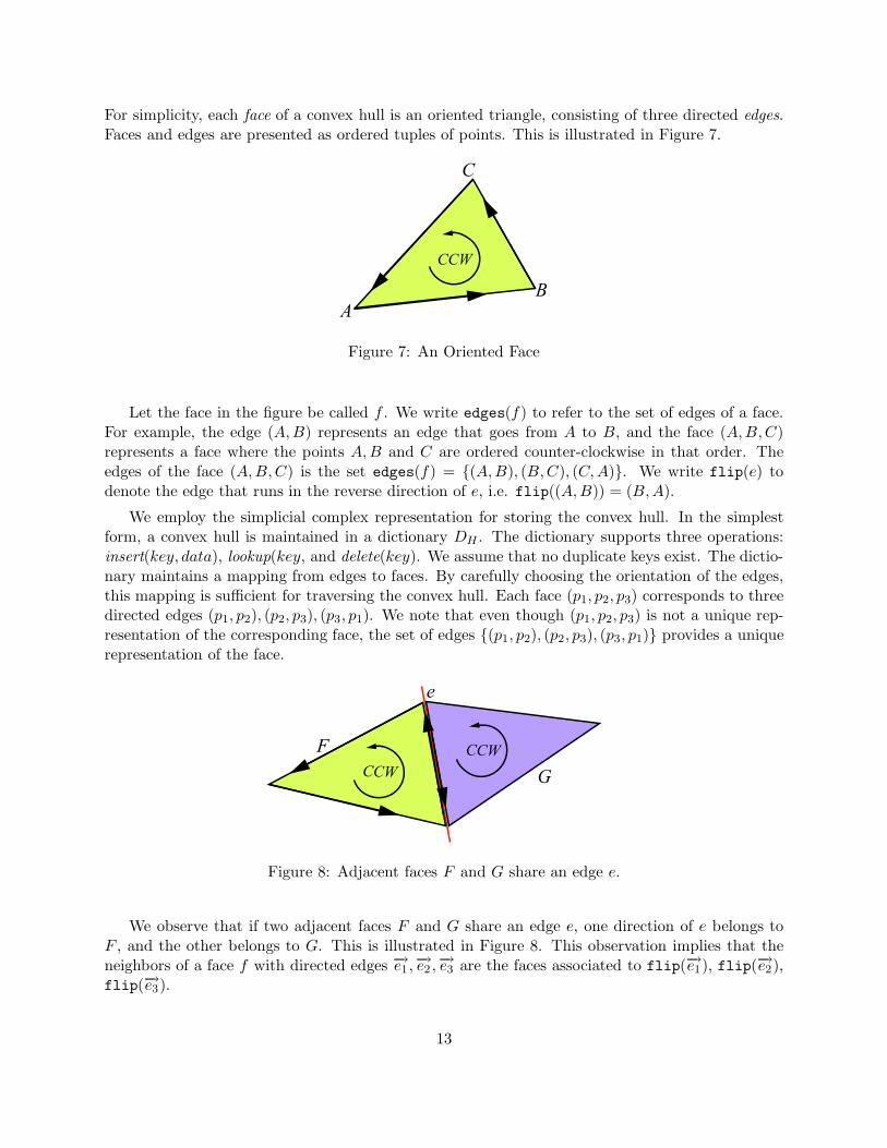
For simplicity, each face of a convex hull is an oriented triangle, consisting of three directed edges.Faces and edges are presented as ordered tuples of points. This is illustrated in Figure 7.

CCW

A

B

C

Figure 7: An Oriented Face

Let the face in the figure be called f . We write edges(f) to refer to the set of edges of a face.For example, the edge (A,B) represents an edge that goes from A to B, and the face (A,B,C)represents a face where the points A,B and C are ordered counter-clockwise in that order. Theedges of the face (A,B,C) is the set edges(f) = (A,B), (B,C), (C,A). We write flip(e) todenote the edge that runs in the reverse direction of e, i.e. flip((A,B)) = (B,A).

We employ the simplicial complex representation for storing the convex hull. In the simplestform, a convex hull is maintained in a dictionary DH . The dictionary supports three operations:insert(key, data), lookup(key, and delete(key). We assume that no duplicate keys exist. The dictio-nary maintains a mapping from edges to faces. By carefully choosing the orientation of the edges,this mapping is sufficient for traversing the convex hull. Each face (p1, p2, p3) corresponds to threedirected edges (p1, p2), (p2, p3), (p3, p1). We note that even though (p1, p2, p3) is not a unique rep-resentation of the corresponding face, the set of edges (p1, p2), (p2, p3), (p3, p1) provides a uniquerepresentation of the face.

CCW

CCW

e

F

G

Figure 8: Adjacent faces F and G share an edge e.

We observe that if two adjacent faces F and G share an edge e, one direction of e belongs toF , and the other belongs to G. This is illustrated in Figure 8. This observation implies that theneighbors of a face f with directed edges −→e1 ,−→e2 ,−→e3 are the faces associated to flip(−→e1), flip(−→e2),flip(−→e3).

13

Facts about Randomized Computation in Computational Geometry. We introducemore notations and definitions and reiterate a lemma of Clarkson and Shor for bounding the numberof objects at conflict with a particular region. Assume that each region is defined by at most bobjects for some b ∈ Z+. Let F i

j(S) denote the subset of regions of F(S) containing exactly theregions that are defined by precisely i objects of S and are at conflict with precisely j objects of S.We further define

F i≤j(S) =

⋃

k≤j

F ik(S) and Fj(S) =

⋃

k∈Z+

Fkj (S)

A r-random sample of a finite set of objects S is an r-subset of S chosen at random (i.e. withprobability 1/

(

nr

)

). We note that the model of equal chance mentioned earlier always yields an|Si|-random sample at the i-th stage.

Let fj(r, S) be the expected size of E[|Fj(R)|], where the expectation is taken over r-randomsamples of S.

Lemma 11 (Clarkson and Shor [CS89])

E[|F i≤j(S)|] = O

(

jif0(bn/jc, S)

Proof: We supply a proof due to Clarkson and Shor [CS89] for completeness. The proof uses therandom-sampling technique. Let R be an r-random sampling of S. First, we note that a regionv ∈ F i

j(S) is free of conflicts with objects in a set R ⊆ O if and only if all i objects defining vbelong to R while all j objects at conflict with v lie elsewhere. That is, Pr(v ∈ F0(R)) is given by:

Pr(v ∈ F0(R)) =

(

n−i−jr−i

)

(

nr

) =(n− i− j)!r!(n − r)!

(n− r − j)!(r − i)!n!≥

1

4

r · · · (r − i + 1)

n · · · (n− i + 1)

The expectation E[|F i0(R)|] is computed as follows.

E[|F i0(R)|] =

n−i∑

j=0

∑

v∈F ij (S)

Pr(v ∈ F0(R)) ≥

j∑

k=0

∑

v∈F ij (S)

Pr(v ∈ F0(R))

≥

( j∑

k=0

∣

∣F ik(S)

∣

∣

)

1

4

r · · · (r − i + 1)

n · · · (n− i + 1)=

∣

∣F i≤j

∣

∣

1

4

r · · · (r − i + 1)

n · · · (n − i + 1)

Therefore,∣

∣

∣F i≤j

∣

∣

∣= O(jif0(bn/jc, S)).

Facts about 3-d Convex Hulls. Few properties of convex hulls in the three-dimensionalspace are worth mentioning. Using the notation presented earlier, we point out that, in the contextof 3D convex hulls, F0(R) is the set of faces of the convex hull of the set R. Thus, f0(r, S) is theexpected number of faces on a r-random sample of S. The following lemma is well-known; we stateit without a proof.

Lemma 12 Assume general position of points. For 3D convex hulls,

f0(r,O) = O(r).

14

Since each face is defined by 3 points, it immediately follows from this lemma and Lemma 11that the expected number of faces at conflict with at most j points is linear in the number of inputpoints.

* * * * * * * *

A Model of Equal Chance. We describe a randomized model for sequences of insertionsand deletions. The model is a variant of the models introduced and studied by Mulmuley [Mul91a,Mul91c, Mul91b], Boissonnatet al. [BDS+92], and Schwarzkopf [Sch91].

In this model, an adversary chooses the universe O and a sequence δ ∈ +,−∗ of a finitelength. The entry δi denotes the action to take place at the i-th step: + for an insert, and −for a delete. The algorithm starts with S0 = ∅ and goes through stages. There are two possibletransitions from Si to Si+1, depending on the value of δi:

• For an insertion, the algorithm picks a point p ∈ O\Si uniformly at random, resulting inSi+1 = Si ∪ p.

• For a deletion, the algorithm picks a point p ∈ Si uniformly at random, resulting in Si+1 =Si\p.

This description implies that Si is equally likely to be any one of the |Si|-subsets of O.

* * * * * * * *

Kinetic Setting. Instead of stationery points, the locations of points in the kinetic settingchange as a function time. The reader is referred to the survey papers of Guibas [Gui04] for acomprehensive treatment of the subject. In a nutshell, the location of a point p is determined as(xp(t), yp(t), zp(t)). The combinatorial structure of interest (convex hull, in this case) is maintainedas the time progresses.

5.2 An Algorithm for Maintaining 3-d Convex Hulls

This section outlines an algorithm for maintaining 3D convex hulls that we dynamize and kinetize.The algorithm is a slight modification of the standard incremental convex hull. Our variant ofincremental convex hull uses the simplicial complex representation and maintains the conflict graphsomewhat differently from the version described in Schwarzkopf et al. [dBSvKO00]. We provide apseudo-code of the algorithm in Algorithm 2.

As typical with most incremental algorithms, the main function (hull) takes a list of points Land constructs the convex hull by incrementally inserting each point. The algorithm assumes thelist L is pre-permuted.

In order to compute the hull efficiently, the algorithm maintains various relations betweenpoints, edges, and faces. As described earlier, the convex hull is maintained as a mapping fromedges to faces. In addition, the algorithm maintains a conflict map and a visibility map. A conflictmap associates each face with a list of points (not yet inserted) that conflicts with the face. A

15

visibility hint provides a partial mapping for which point sees which face. This is a hint rather thana complete mapping for reasons that will soon be apparent.

We say that a point p is at a direct conflict with the face f if the ray −→cp penetrates the facef . Immediately before the insertion of the point with rank i, the following three invariants hold:1) the hull is the convex hull of the points of all points with rank less than i, 2) for any point pj

with j > i, V maps pj to a face, 3) and each face f of the hull has a conflict list consisting of allremaining points with direct conflicts with the face f .

These functions are represented using three different dictionaries: the convex hull dictionary(H), the conflict dictionary (C), and the visibility dictionary (V ). The pseudo-code assumes thatthe hull, the visibility and conflict maps are initialized to contain the convex hull of the first threepoints and the resulting conflict and visibility maps. In addition, the algorithm uses a priorityqueue data structure that supports insert and deleteMin operations.

To insert a point p on the hull, the algorithm first finds a face f that is visible to the point pbeing inserted. The algorithm then checks if f is in the hull. If not, then p is inside the hull, inwhich case the hull remains the same. Otherwise the algorithm calls the rip function to removeall the faces that are visible from p by using one of the edges of the face f . The function returnsthe set of points π that conflict with the removed faces, the boundary edges E of the hull that areadjacent to ripped out faces, and the partial hull H. The region removed from the hull is thentented at p by calling the tent function.

Given a point p, a set of boundary edges E , and a set of points π, the tent function extendsthe hull by inserting the point p to the hull. This requires making a face from each boundary edgeand the point p. For each new face f , the function determines the points π′ that conflict with fand updates the conflict dictionary. The algorithm then identifies the point pm with the minimumrank that conflicts with f and updates the visibility map by mapping the pm to f .

A dynamic algorithm is derived from applying syntactic transformation techniques of self-adjusting computation. By pairing the dynamic algorithm with our kinetic library [ABTV06],we obtain a kinetic algorithm for 3-d convex hull that also supports dynamic changes.

5.3 Analysis of the Algorithm

We present a few facts (and their proofs) about the algorithm, and informally argue about itsefficiency. The input to the algorithm is a permutation of points drawn from a finite universe O.We assume that dynamic changes obey the model of equal chance (described in the preliminaries).Let τ(n) denote the expected number of faces of the convex hull with n points. It is well-knownthat τ(n) = O(n).

Lemma 13 (Constant Degree) Record all edges ever created through the lifetime of an Incre-mental Hull 3D. Create a graph G, whose nodes are the points of O and whose edges are thoseedges. Let d be the average degree of this graph (i.e. d = 1

n

∑

v∈V (G) degG(v). Then,

E[d] = O(1) .

Proof: Consider the degree sum D =∑

v∈V (G) degG(v). For the point being inserted at the i-th

step to the hull, let Di be the increase in the degree. We find that D =∑n

i=1 Di. The lemma

16

Algorithm 2 Modified Incremental Hull 3D

function hull (L) =

while (L 6= nil) do

p ← first (L)case lookupV (p) of

Found(f):(e, , )← edges(f)case lookupH (e) of

Found f:

(π,E) ← rip (p, e)tent (p, π, E)

NotFound: deleteV (p)NotFound:

L ← next (L)

function rip(p, e) =

E ← ∅π ← ∅Q← flipe

while (Q 6= ∅) do

e ← deleteMin(Q)case lookupH (flipe) of

Found(f):if isVisible(p, f) then

π ← π ∪ lookupC(f)(e1, e2, e3)← edgesf

deleteH (e1, f)deleteH (e2, f)deleteH (e3, f)deleteC(f)Q ← Q ∪ e1, e2, e3 \ e

else E ← E ∪ eNotFound:

return (π, E)

function tent(p, π, E) =

for each e = (p1, p2) ∈ E do

f ← (p2, p1, p)π′ ← p ∈ π : −→pcp ∩ f 6= ∅(e1, e2, e3)← edgesf

insertH (e1, f)insertH (e2, f)insertH (e3, f)insertC(f, π′)π ← π\π′

pm ← arg minq∈π′rank(q)deleteV (pm)insertV (pm, f)

follows, as E[Di] = O(1).

Lemma 14 Assume that rank(p∗) < r. Let F be the set of faces “ripped” during the insertionof the point pr. Let F ′ be the set of faces “ripped” during the insertion of the point pr under thepresence of p∗. Then, E[|F∆F ′|] ≤ C/r for some constant C ∈ R

+.

Proof: First, we bound the size of F\F ′. A face f is ripped initially but is not ripped when p∗

is present if and only if p∗ is at conflict with f . Thus, we have F\F ′ = f ∈ CH(Sr−1) : pr, p∗ ⊆

F(f) = f ∈ F2(Sr−1 ∪ pr, p∗) : F(f) = pr, p

∗. According to the model of equal chance, weestablish

E[|F\F ′|] =1

(

|O|r+1

)

∑

R⊆O|R|=r+1

1

r + 1

∑

p∗∈R

1

r

∑

pr∈Rpr 6=p∗

|f ∈ F2(R) : F(f) = pr, p∗|

≤1

r2

1( |O|r+1

)

∑

R⊆O|R|=r+1

|F2(R)| ≤O(τ(r + 1))

r2≤ C1/r

for a suitable C1 ∈ R+.

Then, we approximate the size of F ′\F by observing that f ∈ F ′\F if and only if f is at conflictwith pr and p∗ ∈ Defn(f). Thus, F ′\F = f ∈ CH(Sr−1 ∪ p

∗) : p∗ ∈ Defn(f) and pr ∈ F(f). It

17

follows that

E[|F ′\F |] =1

( |O|r+1

)

∑

R⊆O|R|=r+1

1

r + 1

∑

pr∈R

1

r

∑

p∗∈Rp∗ 6=pr

|f ∈ CH(R\pr) : p∗ ∈ Defn(f) and pr ∈ F(f)|

≤1

( |O|r+1

)

∑

R⊆O|R|=r+1

1

r + 1

∑

pr∈R

3

r|f ∈ CH(R\pr) : pr ∈ F(f)| ≤ C2/r

We remark that f ∈ CH(R\pr) : pr ∈ F(f) ⊆ f ∈ F≤2(R) : pr ∈ F(f).

Lemma 15 Let G be the set of faces “tented” during the insertion of the point pr. Let G′ be definedsimilarly except in the presence of p∗. Then, |G∆G′| ≤ C/i for some constant C ∈ R

+.

The proof is similar to that of the previous lemma and is omitted.

Theorem 16 The algorithm for maintain convex hulls in 3-d outlined in Algorithm 2 is O(logn)-stable with respect to dynamic (and kinetic) changes in the model of equal chance.

Sketch of Proof: We argue that the trace differences for each point being inserted can bethought of as structural differences at the particular step. Following from two previous lemmas, weconclude that the total trace differences is at most

∑nr=1(C1 + C2)/r = O(log n).

We further argue that every kinetic change can be simulated by deleting the relevant pointand re-inserting it. An actual kinetic change is much cheaper than this simulation. ApplyingTheorem 5, we establish that the algorithm is also O(log n)-stable for kinetic changes (assumingthat each point is equally likely to participate in a kinetic event).

5.4 Implementation and Experimental Evaluation

We implemented a variant of the algorithm described earlier. The implementation differs from thedescription in Algorithm 2, as we find that, in practice, the algorithm can perform well even ifthe program-monotonicity assumption is relaxed. The implementation also stores the convex hullin a dynamized treap—an equivalence of an active dictionary. We note that even though Treapsallow for non-exact queries, in the scope of our use, Treaps and active dictionaries provide thesame interface and functionalities. We suspect that an active dictionary will have less overheadthan a Treap, since the dynamic behaviors of our Treap have to pay the overhead of self-adjustingcomputation.

We evaluate the effectiveness of our algorithm through a set of benchmarks, of which two arereported and discussed:

Time for initial run: This experiment measures the total time it takes to run the dynamicversion on a given input. In order to determine the overhead our techniques, we divide thistime by the time for running the static version of the same program.

18

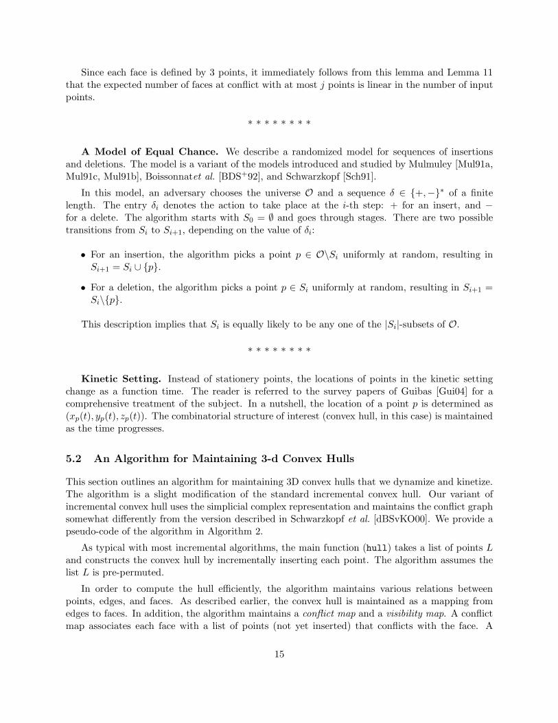
Average time for a deletion/insertion: This experiment mimics a dynamic change in themodel of equal chance discussed earlier. It measures the average time taken to perform aninsertion/deletion. We start by running a self-adjusting application on a given input list. Wethen delete the first element in the input list and perform a change propagation. Next, weinsert the element back into the list and perform a change propagation. We perform thisdelete-propagate-insert-propagate operation for each element. Note that after each delete-propagate-insert-propagate operation, the input list is the same as the original input. Wecompute the average time for an insertion/deletion as the ratio of the total time to thenumber of insertions and deletions (2n for an input of size n).

Figure 9 (left) shows the initial run graph, and the one on the right shows an average time fora dynamic change.

0

0.5

1

1.5

2

2.5

3

3.5

0 200 400 600 800 1000

(Time for From-Scratch Run)

App. + G.C.App.

Ord. App. + G.C.Ord. App.

0

0.01

0.02

0.03

0.04

0.05

0.06

0 200 400 600 800 1000

(Average Time for Insert/Delete)

App. + G.C.App.

Figure 9: Experimental Results for the Convex Hull in 3D

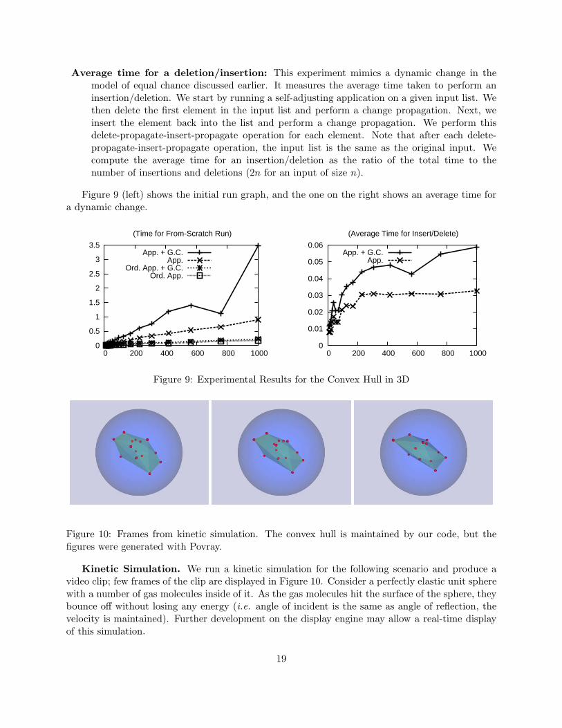
Figure 10: Frames from kinetic simulation. The convex hull is maintained by our code, but thefigures were generated with Povray.

Kinetic Simulation. We run a kinetic simulation for the following scenario and produce avideo clip; few frames of the clip are displayed in Figure 10. Consider a perfectly elastic unit spherewith a number of gas molecules inside of it. As the gas molecules hit the surface of the sphere, theybounce off without losing any energy (i.e. angle of incident is the same as angle of reflection, thevelocity is maintained). Further development on the display engine may allow a real-time displayof this simulation.

19

6 Dynamic Single-Source Shortest-Path

We study the Dijkstra algorithm for computing the single-source shortest-path in a graph. Aspointed out earlier, the distance of the node removed from the priority admits the monotoneproperty. Our study shows that, with an appropriate graph representation, the combination of self-adjusting computation and retroactive priority queue can yield a simple implementation of dynamicsingle-source shortest-path with competitive performance to that of Ramalingam and Reps [RR96]if theirs used a binary heap.

We have implemented the graph represetation and dynamized the Dijkstra algorithm. Our al-gorithm is O(‖δ‖ log‖δ‖)-stable, where δ is the sum of degrees of nodes whose distances change. Wefurther note that our dynamic single-source shortest-path algorithm can be trivially used to devisea dynamic all-pair shortest-path algorithm. The performance, however, may not be comparable tothe best asymptotic bounds to date.

7 Discussions and Conclusion

In this thesis, we present a study of a new data-structuring paradigm and demonstrate somepractical use of it. We show that a number of data structures can be efficiently maintained,delivering tremendous impacts on the design, analysis, and implementation of dynamic and kineticalgorithms. The approach has been proven effective in practice, as supported by the experimentalevidence.

We mention some work in progress and point out certain directions that this work can beextended. There are many other data structures that we have yet to investigate. Even thougha priority queue can simulate a queue, we wonder if it is possible to construct an active queuethat beats O(log T ) runtime. In general, it is natural to find a non-trivial lower-bound for thisclass of data structure. Another interesting data structure to consider is union-find. An efficientactive union-find data structure may enable the development of dynamic minimum spanning treealgorithm based on Prim’s algorithm.

20

A The Triangle Inequality Theorem

Theorem 17 (Triangle Inequality for Change Propagation) Let P be a monotone programwith respect to the class of changes ∆1 and ∆2. Suppose that P is O(f(n)) and O(g(n)) stablefor ∆1 and ∆2, respectively, for some measure n. P is also monotone with respect to the class ofchanges (∆1 ∆2) obtained by composing ∆1 and ∆2, then P is O(f(n)+g(n)) stable for ∆1 o ∆2.

Proof: Let T0, T1, and T2 be the traces of P with some inputs I0, I1, and I2, respectively, suchthat I1 = ∆1(I0), and I2 = ∆2(I1). Note that I2 = (∆2 ∆1)(I0).

To prove the theorem, we will show that the distance δtr (T2, T0) between T2 and T0 is boundedby δtr (T2, T1) + δtr (T1, T0). Let w (·) denote the weight of a vertex. We know by definition thatthe following hold.

δtr (T2, T0) =∑

v∈T2\T0

w (v) +∑

v∈T0\T2

w (v)

δtr (T2, T1) + δtr (T1, T0) =

(

∑

v∈T2\T1

w (v) +∑

v∈T1\T2

w (v)

)

+

(

∑

v∈T0\T1

w (v) +∑

v∈T1\T2

w (v)

)

.

It therefore suffices to show that T2 \T0 ⊆ (T2 \T1)∪ (T1 \T0) and T0 \T2 ⊆ (T0 \T1)∪ (T1 \T2).This follows directly from the following basic property of sets: for any three sets A,B,C, it is truethat (A \ C) ⊆ (A \B) ∪ (B \ C).

We conclude that δtr (T2, T0) ≤ δtr (T2, T1)+ δtr (T1, T0). Since P is O(f(n)) and O(g(n)) stablefor ∆1 and ∆2, respectively, we have δtr ((, T )1 , T0) ∈ O(f(n)) and δtr ((, T )2 , T1) ∈ O(g(n)). Ittherefore follows that P is O(f(n) + g(n)) stable for the changes ∆2 ∆1.

The theorem implies that composing (batching) a constant number of changes does not changethe asymptotic complexity of change propagation with respect to the maximum of the changepropagations with respect to each change.

* * * * * * * *

Remarks. We note that triangle inequality does not hold if the program is not monotonewith respect to the change obtained by composition. For example, if the changes are insertionsand deletions, then they may swap the position of two elements in a list (unless of course theyare restricted to affect the same location). In this case, the program may not be monotone withrespect to a swap, and the theorem will not hold. In fact, it is easy to construct examples of suchprograms. For example, consider some program that takes the input list [1, 2, 3]. Suppose that theprogram traverses the list from head to tail, and performs large amount of work for the item 2 butperforms constant work for all other elements. Now, if we delete 3 perform a change propagationand insert it back before 2 and run change propagation, then both change propagation will takeconstant time (i.e., the inputs are [1, 2, 3], [1, 2], [1, 3, 2]). If instead, we delete 2 and insert it infront of 3 and perform change propagation, then the result for 3 will be found in the memo, but theresult for 2 will not be found—since 3 comes after 2 re-using the result for 3 will delete the resultfor 2. Thus the result for 2 will have to be recomputed requiring possibly non-constant time.

21

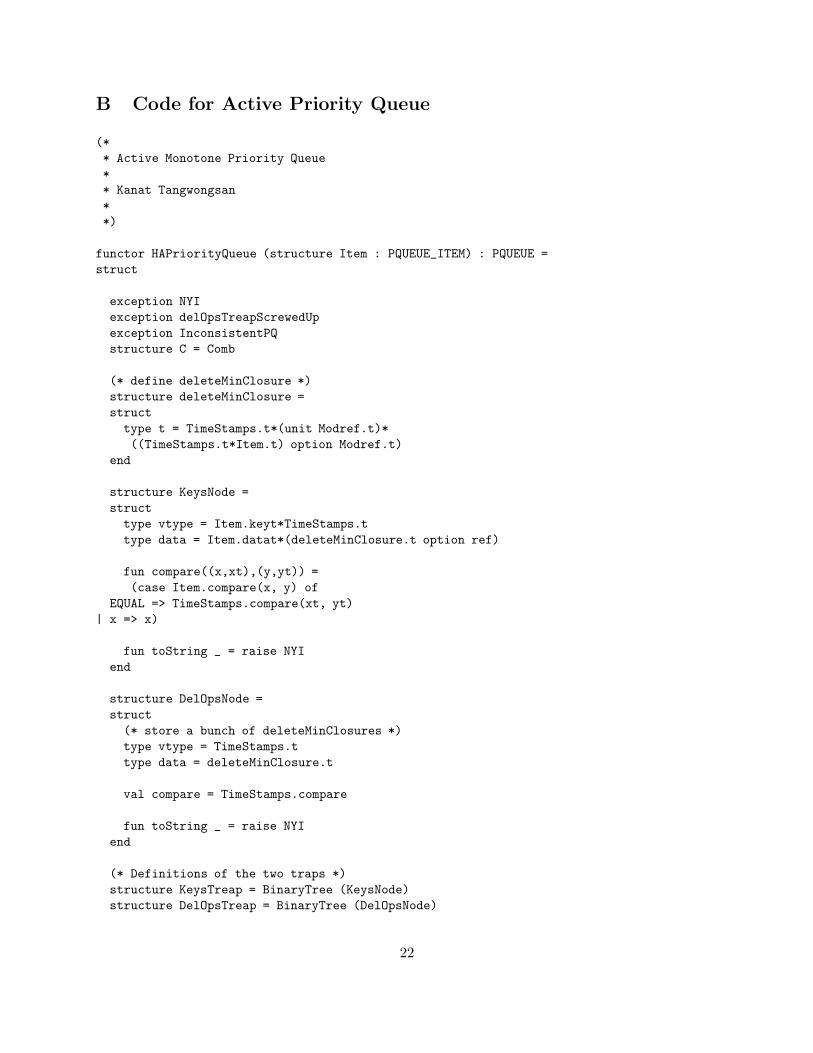
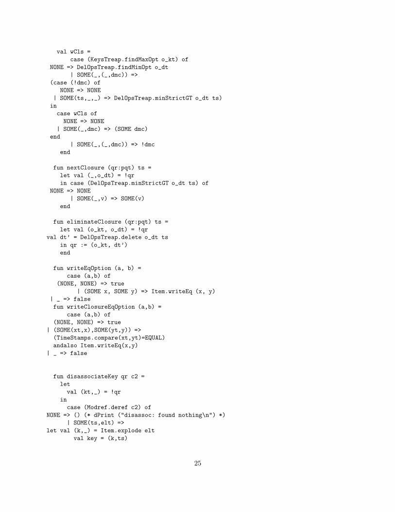
B Code for Active Priority Queue

(*

* Active Monotone Priority Queue

*

* Kanat Tangwongsan

*

*)

functor HAPriorityQueue (structure Item : PQUEUE_ITEM) : PQUEUE =

struct

exception NYI

exception delOpsTreapScrewedUp

exception InconsistentPQ

structure C = Comb

(* define deleteMinClosure *)

structure deleteMinClosure =

struct

type t = TimeStamps.t*(unit Modref.t)*

((TimeStamps.t*Item.t) option Modref.t)

end

structure KeysNode =

struct

type vtype = Item.keyt*TimeStamps.t

type data = Item.datat*(deleteMinClosure.t option ref)

fun compare((x,xt),(y,yt)) =

(case Item.compare(x, y) of

EQUAL => TimeStamps.compare(xt, yt)

| x => x)

fun toString _ = raise NYI

end

structure DelOpsNode =

struct

(* store a bunch of deleteMinClosures *)

type vtype = TimeStamps.t

type data = deleteMinClosure.t

val compare = TimeStamps.compare

fun toString _ = raise NYI

end

(* Definitions of the two traps *)

structure KeysTreap = BinaryTree (KeysNode)

structure DelOpsTreap = BinaryTree (DelOpsNode)

22

type pqt = ((KeysNode.data KeysTreap.t)*

(DelOpsNode.data DelOpsTreap.t)) ref

type t = pqt

type keyt = Item.keyt

type datat = Item.datat

type eltt = Item.t

val dPrint = fn _ => () (*print*) (* fn _ => () *)

fun new () : pqt = ref (KeysTreap.empty, DelOpsTreap.empty)

(**********************************************************************

Utility functions

**********************************************************************)

fun pickUpClosure (qr:pqt) key =

let val (o_kt, _) = !qr

in case KeysTreap.lookup o_kt key of

NONE => NONE

| SOME(_,clsRef) => !clsRef

end

fun eliminateKey (qr:pqt) key =

let val (o_kt,o_dt) = !qr

val kt’ = KeysTreap.delete o_kt key

in qr := (kt’, o_dt)

end

fun scheduleWakeUp cls =

let

val (ts,synA,_) = cls

in case TimeStamps.compare (ts, !Modref.now) of

LESS => ()

| _ => C.iwrite’ (fn _ => false) synA ()

end

fun doRemoveInsert (qr:pqt) x () =

let val wCls : deleteMinClosure.t option = pickUpClosure qr x

(* val () = print "eliminating an insert\n" *)

val () = eliminateKey qr x

in case wCls of

NONE => ()

| SOME(cls) => scheduleWakeUp cls

end

(* NOTE: fetchMinAtTime has a side-effect of removing all "future"

* insertions whose keys are bigger the smallest element not yet

23

* used

*)

fun fetchMinAtTime (qr:pqt) time : (KeysNode.vtype*KeysNode.data) option =

let

fun findMin pvMinItem pvTs : (KeysNode.vtype*KeysNode.data) option =

let val (o_kt, o_dt) = !qr

val curMin =

let val (lastKey, _) = Item.explode pvMinItem

in KeysTreap.minStrictGT o_kt (lastKey, pvTs)

end

in case curMin of

NONE => NONE

| SOME(wKey as (k,curMinTs),(v,_)) =>

(case TimeStamps.compare (curMinTs, time) of

LESS => curMin

| _ =>

let val () = dPrint "fetchMinAtTime: deleting out of time key\n"

in (doRemoveInsert qr wKey ();

findMin (Item.implode(k,v)) curMinTs)

end)

(* | _ => curMin*)

end

val (o_kt, o_dt) = !qr

val prevDelMin : (DelOpsNode.vtype*DelOpsNode.data) option =

DelOpsTreap.maxStrictLT o_dt time

in

case prevDelMin of

(*(dPrint ("no prev dM\n");KeysTreap.findMinOpt o_kt)*)

NONE => (case (KeysTreap.findMinOpt o_kt) of

NONE => NONE

| SOME(wMin as (wKey as (_,ts),_)) =>

(case TimeStamps.compare (ts, time) of

LESS => SOME(wMin)

| _ => (doRemoveInsert qr wKey ();

fetchMinAtTime qr time)))

| SOME(_,(_,_,dm)) =>

(case (Modref.deref dm) of

NONE => NONE

| SOME(ts,lastMin) => findMin lastMin ts)

end

fun findBiggerKey (qr:pqt) key =

let val (o_kt,o_dt) = !qr

(* val tl = map (fn (x,_) => x) (KeysTreap.toListPre o_kt)

val str = foldr (fn (x,s) => (Item.keyToString x)^" "^s) "" tl

val () = dPrint (str^"\n")*)

in case KeysTreap.minStrictGT o_kt key of

NONE => (* find the NONE value *)

let

24

val wCls =

case (KeysTreap.findMaxOpt o_kt) of

NONE => DelOpsTreap.findMinOpt o_dt

| SOME(_,(_,dmc)) =>

(case (!dmc) of

NONE => NONE

| SOME(ts,_,_) => DelOpsTreap.minStrictGT o_dt ts)

in

case wCls of

NONE => NONE

| SOME(_,dmc) => (SOME dmc)

end

| SOME(_,(_,dmc)) => !dmc

end

fun nextClosure (qr:pqt) ts =

let val (_,o_dt) = !qr

in case (DelOpsTreap.minStrictGT o_dt ts) of

NONE => NONE

| SOME(_,v) => SOME(v)

end

fun eliminateClosure (qr:pqt) ts =

let val (o_kt, o_dt) = !qr

val dt’ = DelOpsTreap.delete o_dt ts

in qr := (o_kt, dt’)

end

fun writeEqOption (a, b) =

case (a,b) of

(NONE, NONE) => true

| (SOME x, SOME y) => Item.writeEq (x, y)

| _ => false

fun writeClosureEqOption (a,b) =

case (a,b) of

(NONE, NONE) => true

| (SOME(xt,x),SOME(yt,y)) =>

(TimeStamps.compare(xt,yt)=EQUAL)

andalso Item.writeEq(x,y)

| _ => false

fun disassociateKey qr c2 =

let

val (kt,_) = !qr

in

case (Modref.deref c2) of

NONE => () (* dPrint ("disassoc: found nothing\n") *)

| SOME(ts,elt) =>

let val (k,_) = Item.explode elt

val key = (k,ts)

25

in case (KeysTreap.lookup kt key) of

NONE => ()

| SOME(_,mr) =>

(case (!mr) of

NONE => ()

| SOME(_) => mr := NONE)

end

end

fun grabKey (qr:pqt) (kk:KeysNode.vtype) (nc:deleteMinClosure.t) =

let

val (kt,_) = !qr

(* val () = dPrint "grabKey.. init\n" *)

in

case (KeysTreap.lookup kt kk) of

NONE => raise InconsistentPQ

| SOME(_,mr) =>

(case (!mr) of

NONE => mr := SOME(nc)

| SOME(cls) =>

let (* val () = dPrint "grabKey: SOME/cls\n" *)

(* val () = disassociateKey cls*)

val () = scheduleWakeUp cls

val () = mr := (SOME nc)

in ()

end)

end

(***********************************************************************)

fun c2reader c2 =

(case (Modref.deref c2) of

NONE => "NONE"

|SOME (_,d) => let val (k,v) = Item.explode d

in "SOME("^(Item.keyToString k)^")"

end) handle _ => "undef."

fun clsToHolder cls =

let val (_,_,c2) = cls

in

c2reader c2

end

(**********************************************************************

Action components

**********************************************************************)

fun action_removeInsert (qr:pqt) x () = doRemoveInsert qr x ()

fun action_removeDelMin (qr:pqt) ts () =

let val wCls : deleteMinClosure.t option = nextClosure qr ts

26

(* val () = print "eliminating a delMin\n" *)

val () = eliminateClosure qr ts

in case wCls of

NONE => ()

| SOME(cls) => scheduleWakeUp cls

end

fun action_addInsert (qr:pqt) x =

let

val (o_kt, o_dt) = !qr

val (k, v) = Item.explode x

(* val () = dPrint ("insert: "^(Item.keyToString k)^"\n") *)

val insTime = Modref.insertTime ()

val keyPack = (k, insTime)

val () = TimeStamps.setInv (insTime, action_removeInsert qr keyPack)

val () = (case (findBiggerKey qr keyPack) of

NONE => () (* dPrint ("none to wake up\n") *)

| SOME(cls) =>

let

(* val () = dPrint ("call swaking up..who’s holding"^(clsToHolder cls)^"\n") *)

in scheduleWakeUp cls

end)

val hv = (v, ref NONE)

val kt’ = KeysTreap.insert o_kt (keyPack,hv)

in

qr := (kt’, o_dt)

end

fun action_addDelMin (qr:pqt) =

let

val (synA,synB,outputM) = (Modref.new (), Modref.empty (), Modref.empty())

val delMinTime = Modref.insertTime ()

val () = TimeStamps.setInv (delMinTime, action_removeDelMin qr delMinTime)

val (kt,dt) = !qr

val closure = (delMinTime,synA,synB)

val key = delMinTime

val dt’ = DelOpsTreap.insert dt (key,closure)

val () = qr := (kt, dt’)

fun fwrap_pre () =

C.iread synA (fn () =>

let

(* precond: *)

(* val () = dPrint "i am up\n" *)

(* val (keys,_)= !qr

val tl = map (fn ((x,_),_) => x) (KeysTreap.toListPre keys)

val str = foldr (fn (x,s) => (Item.keyToString x)^" "^s) "" tl

27

val () = dPrint (str^"\n") *)

val curMinCls : (TimeStamps.t*Item.t) option =

(case (fetchMinAtTime qr delMinTime) of (* should be delMinTime not now*)

NONE => NONE

| SOME((k,ts),(v,_)) =>

let (*val () = dPrint ("curmin is"^(Item.keyToString k)^"\n") *)

val () = if TimeStamps.compare(ts, delMinTime) = LESS then

()

else raise Crap

in SOME(ts, Item.implode (k,v))

end)

(* val () = dPrint ("before writing to c2: originally c2 = "^(c2reader c2)^"\n")*)

val () =

(if (writeClosureEqOption (curMinCls, Modref.deref synB)) then

()

else disassociateKey qr synB) handle _ => ()

in

C.iwrite’ writeClosureEqOption synB curMinCls

end)

fun fwrap_post () =

C.iread synB (fn tvalue =>

let

(* val () = dPrint "c2 invoked\n" *)

val closure = (delMinTime,synA,synB)

val () = (case tvalue of

NONE => ()

| SOME(ts,kk) =>

let val (k’,_) = Item.explode kk

in grabKey qr (k’,ts) closure

end)

(* val () = dPrint "postc2:y\n" *)

val value = case tvalue of

NONE => NONE

| SOME(_,x) => SOME(x)

(* val () = dPrint "transfering to c3\n" *)

in

C.iwrite’ writeEqOption outputM value

end)

val _ = fwrap_pre ()

val _ = fwrap_post ()

in

outputM

end

fun insert qr x = action_addInsert qr x

fun deleteMin (qr:pqt) = action_addDelMin qr

end

28

References

[ABB+05] Umut A. Acar, Guy E. Blelloch, Matthias Blume, Robert Harper, and Kanat Tang-wongsan. A library for self-adjusting computation. In ACM SIGPLAN Workshop onML, 2005.

[ABBT06] Umut A. Acar, Guy E. Blelloch, Matthias Blume, and Kanat Tangwongsan. Anexperimental analysis of self-adjusting computation, 2006. To Appear in the Pro-ceedings of the ACM SIGPLAN Conference on Programming Language Design andImplementation.

[ABH02] Umut A. Acar, Guy E. Blelloch, and Robert Harper. Adaptive functional program-ming. In Proceedings of the 29th Annual ACM Symposium on Principles of Program-ming Languages, pages 247–259, 2002.

[ABH+04] Umut A. Acar, Guy E. Blelloch, Robert Harper, Jorge L. Vittes, and Shan Leung Mav-erick Woo. Dynamizing static algorithms, with applications to dynamic trees andhistory independence. In SODA ’04: Proceedings of the fifteenth annual ACM-SIAMsymposium on Discrete algorithms, pages 531–540, 2004.

[ABTV06] Umut A. Acar, Guy E. Blelloch, Kanat Tangwongsan, and Jorge Vittes. Kineticalgorithms via self-adjusting computation. Technical Report CMU-CS-06-115, De-partment of Computer Science, Carnegie Mellon University, March 2006.

[Aca05] Umut A. Acar. Self-Adjusting Computation. PhD thesis, Department of ComputerScience, Carnegie Mellon University, May 2005.

[BCD+02] Michael A. Bender, Richard Cole, Erik D. Demaine, Martin Farach-Colton, and JackZito. Two simplified algorithms for maintaining order in a list. In Lecture Notes inComputer Science, pages 152–164, 2002.

[BDS+92] Jean-Daniel Boissonnat, Olivier Devillers, Ren Schott, Monique Teillaud, and Mari-ette Yvinec. Applications of random sampling to on-line algorithms in computationalgeometry. Discrete & Computational Geometry, 8:51–71, 1992.

[BGH97] Julien Basch, Leonidas J. Guibas, and John Hershberger. Data structures for mobiledata. In SODA’97, pages 747–756, 1997.

[BJ02] Gerth Stolting Brodal and Riko Jacob. Dynamic planar convex hull. In Proceedingsof the 43rd Annual IEEE Symposium on Foundations of Computer Science, pages617–626, 2002.

[BY98] Jean-Daniel Boissonnat and Mariette Yvinec. Algorithmic Geometry. CambridgeUniversity Press, 1998.

[Car02] Magnus Carlsson. Monads for incremental computing. In Proceedings of the seventhACM SIGPLAN international conference on Functional programming, pages 26–35.ACM Press, 2002.

29

[Cha06] Timothy M. Chan. A dynamic data structure for 3-d convex hulls and 2-d nearestneighbor queries. In SODA ’06: Proceedings of the seventeenth annual ACM-SIAMsymposium on Discrete algorithm, pages 1196–1202, New York, NY, USA, 2006. ACMPress.

[CS89] Kenneth L. Clarkson and Peter W. Shor. Applications of random sampling in com-putational geometry,II. Discrete and Computational Geometry, 4(1):387–421, 1989.

[dBSvKO00] Mark de Berg, Otfried Schwarzkopf, Marc van Kreveld, and Mark Overmars. Com-putational Geometry: Algorithms and Applications. Springer-Verlag, 2000.

[DIL04] Erik D. Demaine, John Iacono, and Stefan Langerman. Retroactive data structures.In Proceedings of the 15th Annual ACM-SIAM Symposium on Discrete Algorithms(SODA 2004), pages 274–283, New Orleans, Louisiana, January 11–13 2004.

[DRT81] Alan Demers, Thomas Reps, and Tim Teitelbaum. Incremental evaluation of at-tribute grammars with application to syntax directed editors. In Proceedings of the8th Annual ACM Symposium on Principles of Programming Languages, pages 105–116, 1981.

[DS87] P. F. Dietz and D. D. Sleator. Two algorithms for maintaining order in a list. InProceedings of the 19th ACM Symposium on Theory of Computing, pages 365–372,1987.

[Gra72] R. L. Graham. An efficient algorithm for determining the convex hull of a fineteplanar set. Information Processing Letters, 1:132–133, 1972.

[Gui04] L. Guibas. Modeling motion. In J. Goodman and J. O’Rourke, editors, Handbook ofDiscrete and Computational Geometry, pages 1117–1134. Chapman and Hall/CRC,2nd edition, 2004.

[Mul91a] Ketan Mulmuley. Randomized multidimensional search trees (extended abstract):dynamic sampling. In Proceedings of the seventh annual symposium on Computationalgeometry, pages 121–131. ACM Press, 1991.

[Mul91b] Ketan Mulmuley. Randomized multidimensional search trees: Further results in dy-namic sampling (extended abstract). In Proceedings of the 32nd Annual IEEE Sym-posium on Foundations of Computer Science, pages 216–227, 1991.

[Mul91c] Ketan Mulmuley. Randomized multidimensional search trees: Lazy balancing anddynamic shuffling (extended abstract). In Proceedings of the 32nd Annual IEEESymposium on Foundations of Computer Science, pages 180–196, 1991.

[Ove83] Mark H. Overmars. The Design of Dynamic Data Structures. Springer, 1983.

[OvL81] Mark H. Overmans and Jan van Leeuwen. Maintenance of configurations in the plane.Journal of Computer and System Sciences, 23:166–204, 1981.

[PT89] William Pugh and Tim Teitelbaum. Incremental computation via function caching.In Proceedings of the 16th Annual ACM Symposium on Principles of ProgrammingLanguages, pages 315–328, 1989.

30

[RR96] G. Ramalingam and T. Reps. On the computational complexity of dynamic graphalgorithms. Theoretical Computer Science, 158(1–2):233–277, 1996.

[Sch91] O. Schwarzkopf. Dynamic maintenance of geometric structures made easy. In In Pro-ceedings of the 32nd Annual IEEE Symposium on Foundations of Computer Science,pages 197–206, 1991.

31