active fault-tolerant control of a cstr system based on ... · therefore is widely used in the...

Abstract—In this paper, we present an active fault-tolerant

control method for a continuous stirred tank reactor (CSTR)

system. In the proposed method, a piecewise affine (PWA)

form of the system is modeled in both the normal and fault

situations, and then an active fault-tolerant controller is

designed using an explicit model predictive control algorithm.

By this way, the control objective can be achieved simply by

changing the controller parameters without re-computing the

controller online when the system faults occur. So the method

greatly reduces the computational burden and has a better

real-time performance. Finally, simulation experiments for the

system exposed to multiple sensor or actuator faults are

carried out and show the effectiveness of the method.

Index Terms—piecewise affine model, active fault-tolerant

control, explicit model predictive control, continuous stirred

tank reactor system.

I. INTRODUCTION

HE continuous stirred tank reactor (CSTR) system

plays a vital role in the polymerization reaction and

therefore is widely used in the chemical industry. However,

once faults of the system occur, such as actuator or sensor

faults, it will lead to poor quality and low yield of the

products. So finding an appropriate fault-tolerance control

technique of the system is very necessary and important.

The fault-tolerant control technique is capable of

achieving the system acceptable performance and stability

properties in both the normal and fault situations and can be

classified into two types: passive and active. In the passive

fault-tolerant control approach, it takes into account of all

the expected component faults during the design of a

controller, so that the system can maintain its expected

performance when these faults occur. It doesn’t change but

uses the same robust controller during the whole operation

period which will sacrifice parts of system performance and

have great conservativeness. This method can be found in

[1-4]. Contrary to the passive approach, the active approach

uses a detection and diagnosis module (FDD) to get the

real–time information of system faults and changes the

control strategies with types of the faults, such as

reconfiguration of the current controller, re-scheduling of

Manuscript received January 16, 2016; revised April 11, 2016. This

work was supported by the Shandong Provincial Natural Science Foundation of China (No. 2013ZRE28089).

Yuhong Wang is a professor in the College of Information and Control

Engineering, China University of Petroleum (East China), Qingdao 266580, PR China (e-mail:[email protected]).

Pu Yang is with the College of Information and Control Engineering,

China University of Petroleum (East China), Qingdao 266580, PR China (e-mail:[email protected]).

the control law and so on. So it is able to achieve the

control goal even in the situation of unexpected system

failure. This method is received more attention and can be

found in [5-9].

For the CSTR system, several fault-tolerant control

methods have already been proposed. In [10], a fault-

tolerant controller is designed for a CSTR system subject to

constraints and sensor data losses faults via a

reconfiguration-based approach which can always preserve

closed-loop stability. In [11], a CSTR system is modeled in

an adaptive neural network form. When faults occur, it

compensates the fault effects by employing an auto-tuning

PID controller based on the established model. In [12], it

proposes a method to design a controller on the basis of an

adaptive learning and a switching function mechanism and

then applies this method to a CSTR system with actuator

faults successfully. In [13], it provides a new fault-tolerant

method to control a CSTR system with multiple control

failures relying on the coordination of a multi-loop

proportional controller and a decentralized unconditionally

stabilizing controller. However, these research results are

mainly concentrated in passive fault-tolerant control of the

CSTR system. For active methods, to the knowledge of the

authors it is still lacking in studies. In this paper, an active

fault-tolerant control method is proposed for a CSTR

system. As some literatures, such as [14-18], has already

presented fault detection and diagnosis strategies and their

available for the CSTR system, we mainly focus our

attention on active fault-tolerant controller design.

The idea of the proposed method combines active

fault-tolerant control strategies with explicit model

predictive control algorithms based on piecewise affine

(PWA) model. In the method, a CSTR system is modeled in

a PWA form which not only describes the system

characteristics very well, but is convenient to be used to

design the controller as well. Then an active fault-tolerant

controller is designed using an explicit model predictive

control approach and it can remain stable and feasible by

properly choosing the design parameters. The method

enables the system to make corresponding response to

faults, mainly considering actuator or sensor faults here,

quickly. The rest of this paper is organized as follows. In

Section II, a brief description of PWA model and a PWA

form of the CSTR system are presented. In Section III, an

active fault-tolerant control algorithm is researched in detail.

In Section IV, the proposed method is applied to the CSTR

system subjected to actuator and sensor faults. Finally,

conclusions are drawn in Section V.

Active Fault-tolerant Control of a CSTR System

Based on PWA Model

Yuhong Wang, and Pu Yang, Member, IAENG

T

IAENG International Journal of Applied Mathematics, 46:3, IJAM_46_3_13

(Advance online publication: 26 August 2016)

______________________________________________________________________________________

II. CSTR SYSTEM BASED ON PWA MODEL

A. PWA Model

PWA model is a typical model which contains a finite

number of continuous dynamic submodels and can be

switched among the submodels according to a specific

switching law. It can describe a large number of physical

systems very well, especially for nonlinear systems. In the

model, the extended state+input space is partitioned into

several polyhedral regions and each region is associated

with a different linear state-update equation. It can be

expressed by the following form:

1 ( ), ( )

( )

( )1, ,

PWA i i i

i i i

i

x k f x k u k A x k B u k f

y k C x k D u k g

x kif i s

u k

(1)

where 0k , nx is the state, mu andpy is the

input and the output respectively. 1

,s

i ixix u H x

, 1, ,iu iH u K i s is the polyhedral partition of the sets

which are in the extended space , n mx u . It should be

noted that linear state and input constraints in the form of

Kx k Lu k M can be easily incorporated in the

description of i [25].

B. CSTR System in PWA Form

In this paper, a schematic of a standard two-state CSTR

system is shown in Figure 1.

Fig. 1. Continuous stirred tank reactor system

It is assumed that a single irreversible, exothermic

reaction A B occurs in this reactor. With concentration of

A ( AC ) and the reactor temperature ( T ) as states

1 2[ , ]Tx x x , the coolant temperature ( cfT ) as input u ,

AC as output y , a set of nonlinear equations can be

obtained to describe the system as follows according to

[20,22]:

1

1 2 1 1

2

1 2 2 2

1

( ) ( )

( ) ( )

f

f

dxx x q x x

dt

dxx x q x u qx

dt

y x

Where2

2

2

( ) exp( )1 /

xx

x

and the ranges of the

variables are [0,1] [0,6]x , [ 2,2]u . Values of parameters

in the nonlinear equations are shown in Table 1.

TABLE I

VALUES OF PARAMETERS

q 1 fx 2 fx

20.0 0.072 1.0 8.0 0.3 1.0 0

Apparently, the system is highly nonlinear and multi-

operating points. If it is modeled in PWA form, these

characteristics can be well captured.

For the nominal parameters, it has three steady states

(steady operating points):1

(0.856,0.886)sx , 2

0.5528,sx

2.7517 ,3

(0.2353,4.7050)sx . By linearizing the system

around each steady state point and then discretizing it with

a sampling time of 0.1 sec, we can get the PWA model of

the CSTR system as follows：

1

2

0.8889 0.0123 0.0002 0.1060( ) ( ) ,

0.1254 0.9751 0.0296 0.0852

0.8241 0.0340 0.0005 0.1907( 1) ( ) ( ) ,

0.6365 1.1460 0.0322 0.7537

0.6002 0.0463

2.4016 1.2430

x k u k x

x k x k u k x

3

0.0007 0.3119( ) ( ) ,

0.0338 1.7083

1 0

x k u k x

y k x k

where 3

1, , 1,2,3i ix iu ii

x u H x H u K i

is the

polyhedral partition of the sets of the state+input space.

, , , 1,2,3ix iu iH H K i are, respectively, 6 2 , 6 1 , 6 1

corresponding matrices.

III. ACTIVE FAULT-TOLERANT CONTROL ALGORITHM

A. Active Fault-tolerant Control Based on PWA Model

Active fault-tolerant control of a system with PWA form

achieves control objectives by way of changing control

strategies when system faults, mainly considering actuator

or sensor faults here, are detected. In detail, it needs to use

a FDD module to real-time monitor the system and get the

information of the faults in time once it occurs. Then the

information is passed to a supervision module and

corresponding control actions are subsequently taken to

accommodate and recover the faulty system according to

the fault messages. The general structure of this active

fault-tolerant control system can be depicted in Figure 2.



______________________________________________________________________________________

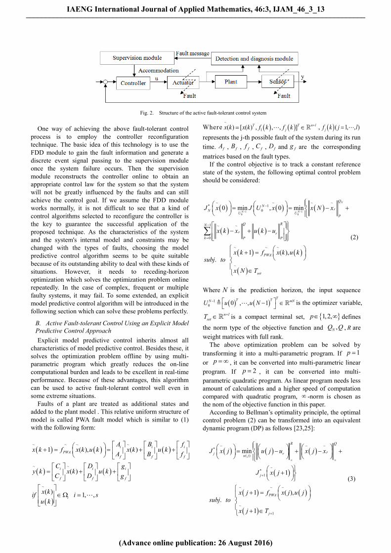
One way of achieving the above fault-tolerant control

process is to employ the controller reconfiguration

technique. The basic idea of this technology is to use the

FDD module to gain the fault information and generate a

discrete event signal passing to the supervision module

once the system failure occurs. Then the supervision

module reconstructs the controller online to obtain an

appropriate control law for the system so that the system

will not be greatly influenced by the faults and can still

achieve the control goal. If we assume the FDD module

works normally, it is not difficult to see that a kind of

control algorithms selected to reconfigure the controller is

the key to guarantee the successful application of the

proposed technique. As the characteristics of the system

and the system's internal model and constraints may be

changed with the types of faults, choosing the model

predictive control algorithm seems to be quite suitable

because of its outstanding ability to deal with these kinds of

situations. However, it needs to receding-horizon

optimization which solves the optimization problem online

repeatedly. In the case of complex, frequent or multiple

faulty systems, it may fail. To some extended, an explicit

model predictive control algorithm will be introduced in the

following section which can solve these problems perfectly.

B. Active Fault-tolerant Control Using an Explicit Model

Predictive Control Approach

Explicit model predictive control inherits almost all

characteristics of model predictive control. Besides these, it

solves the optimization problem offline by using multi-

parametric program which greatly reduces the on-line

computational burden and leads to be excellent in real-time

performance. Because of these advantages, this algorithm

can be used to active fault-tolerant control well even in

some extreme situations.

Faults of a plant are treated as additional states and

added to the plant model . This relative uniform structure of

model is called PWA fault model which is similar to (1)

with the following form:

~ ~ ~ ~

~ ~

~

1 ( ), ( )

( )

( )1, ,

i i i

PWA

f f f

i i i

f f f

i

A B fx k f x k u k x k u k

A B f

C D gy k x k u k

C D g

x kif i s

u k

Where ~

1( ) [ ( ) , , , ]T T n l

jx k x k f k f k , ( 1, , )jf k j l

represents the j-th possible fault of the system during its run

time. fA , fB , ff , fC , fD and fg are the corresponding

matrices based on the fault types.

If the control objective is to track a constant reference

state of the system, the following optimal control problem

should be considered:

1 10 0

~ ~ ~ ~* 1

0

1 ~ ~

0

~ ~ ~

~

0 min , 0 min

1 ( ),.

N

N N

Q

NrN

U Up

Q RN

r r

k P P

PWA

set

J x J U x x N x

x k x u k u

x k f x k u ksubj to

x N T

(2)

Where N is the prediction horizon, the input sequence

1

0 0 , , 1T

T TN mNU u u N

is the optimizer variable,

n l

setT is a compact terminal set, 1,2,p defines

the norm type of the objective function and ,NQ Q , R are

weight matrices with full rank.

The above optimization problem can be solved by

transforming it into a multi-parametric program. If 1p

or p , it can be converted into multi-parametric linear

program. If 2p , it can be converted into multi-

parametric quadratic program. As linear program needs less

amount of calculations and a higher speed of computation

compared with quadratic program, -norm is chosen as

the nom of the objective function in this paper.

According to Bellman’s optimality principle, the optimal

control problem (2) can be transformed into an equivalent

dynamic program (DP) as follows [23,25]:

~ ~ ~*

( )

~*

1

~ ~ ~

~

1

min

1

1 ( ),.

1

R Q

rj ru j

j

PWA

j

J x j u j u x j x

J x j

x j f x j u jsubj to

x j T

(3)

Fig. 2. Structure of the active fault-tolerant control system



______________________________________________________________________________________

Where ~ ~ ~

*

NQ

rNJ x N x N x

, N setT T . For each j

1, , 1j N , ~ ~

1, ,n l

j PWA jT x j u j f x j u j T

is the set of all states which make the problem (3) feasible.

If we utilize an inverse-order-solving method to solve the

above DP problem, for each iteration step, it can be

converted into several problems with the form given by the

following:

~ ~*

~

min ,

.

T

zJ x J z x f z

subj to Gz E x W

Where ~ ~

x x k . f , G , E and W are, respectively, suitable

constant matrices easily obtained from Q , R . It is

essentially a multi-parametric linear program if ~

x is

treated as parameters and z as the optimization vector.

According to [24,25], the solutions to the above

multi-parametric linear programs have a PWA form:

~ ~ ~

* ( ) , , 1, ,k k k k

i i iu x k F x k G if x k P i N

Wherek

iP is a polyhedral partition of the set of feasible

states ~

x k including system states and fault states and kN

is the number of k

iP at each iteration step 0, , 1k N .

Then, an explicit active fault-tolerant controller is obtained

by 0k . The whole process of designing the controller can

be done offline.

For online computation, it just needs to decide the

position of the current state in the controller partition and

then evaluate the corresponding piecewise affine function.

If faults of the system occur, it only requires to change the

controller parameters with the fault type which is detected

by the FDD module. The architecture of the proposed

active fault-tolerant scheme can be depicted in Figure 3.

Note that as the system faults which are treated as

additional states increase the state dimension, the explicit

controller may have a large numbers of partitions and that

can lead to bad real-time perfermance. Countering this

problem,a bounding box search tree method is proposed.

The algorithm requires three steps. First, a bounding box

search tree is constructed according to [28]. Secondly,

traverse the tree from the root node to a leaf node to find

partitions possibly containing the current state, and then

search among these candidate partitions sequentially to

determine the exact partition. Thirdly, evaluate the

corresponding piecewise affine function to obtain the

optimal control input and apply it to the system. By this

way, the speed of the online calculation is significantly

improved at the cost of a low additional memory storage

demand and a very short pre-computation time.

In the proposed active fault-tolerant control method, the

relationship between the states (including intrinsic states

and fault states) and the input is explicit, so it doesn’t need

to repeatedly solve optimization problem online even in the

fault condition. It also ensures the closed loop stability via

choosing the proper design conditions, such as terminal set,

prediction horizon and weight matrices. Moreover, the

supervision module is well-placed to be embedded in the

explicit controller which makes the whole system more

simple and applicable.

IV. SIMULATION RESULTS

The CSTR system needs to work at different operating

points in order to produce necessary products. In this paper,

we choose 1s

x as the operating point and make the system

ultimately work at this steady point from an arbitrary initial

state even in the condition of actuator or sensor fault by

using the proposed active fault-tolerant method.

Here actuator faults mainly cause a change of the coolant

temperature range to the range where the actuator is still

working. If this kind of fault occurs, the FDD module will

pass the new range of the coolant temperature to the

controller which subsequently makes a corresponding

response to accommodate and recover the faulty system. It

supposes the system initial state is 0 0.3,4.5x , 1 is the

upper bound of the actuator and 2 is the lower bound.

Add 1 2

Tf to the system states as additional

states and then establish a fault model. When system runs

without faults, 1 2 and 2 2 , that is to say [ 2,2]u .

The simulation results are shown in Figure 4 and Figure 5.

Fig. 3. Structure of the active fault-tolerant control system based on explicit model predictive control approach



______________________________________________________________________________________

Fig. 4. Projection of the controller partition on 1 2,x x plane cut

through 1 2 , 2 2

Fig. 5. Evolution of the states and input in the normal condition

If the actuator faults occur during operation, we suppose

they are detected by the FDD module at sample time

10k , 20k and 22k , which cause the coolant

temperature range to change to [ 1.5,1.5] , [ 1,1] and

[ 0.5,0.5] respectively. The simulation results are shown

in Figure 6-9.


through 1 1.5 , 2 1.5


through 1 1 , 2 1


through 1 0.5 , 2 0.5

Fig. 9. Evolution of the states and input under the actuator fault

condition. The red dash dot line represents real-time constraints of the

input during the whole control process.

The explicit active fault-tolerant controller has 6049

polyhedral partitions with 94 different control laws. Figure

4 and Figure 6-8 show projections of the controller

partition on two states ,AC T cutting through 1 2,

2, 2 , 1 2, 1.5, 1.5 , 1 2, 1, 1 and 1 2,

0.5, 0.5 respectively. Figure 5 shows the system can



______________________________________________________________________________________

ultimately work at the steady point from the initial state and

the whole regulation process is rather fast and smooth.

Figure 9 shows the controller can quickly make

corresponding remedial actions to correct and recover the

system with multiple actuator faults occurrence at a short

interval and ensure the control objective is still achieved. In

this situation, the whole online control process takes only

3.49 seconds, that is to say, merely needs 0.0349 seconds

on average at each sampling time.

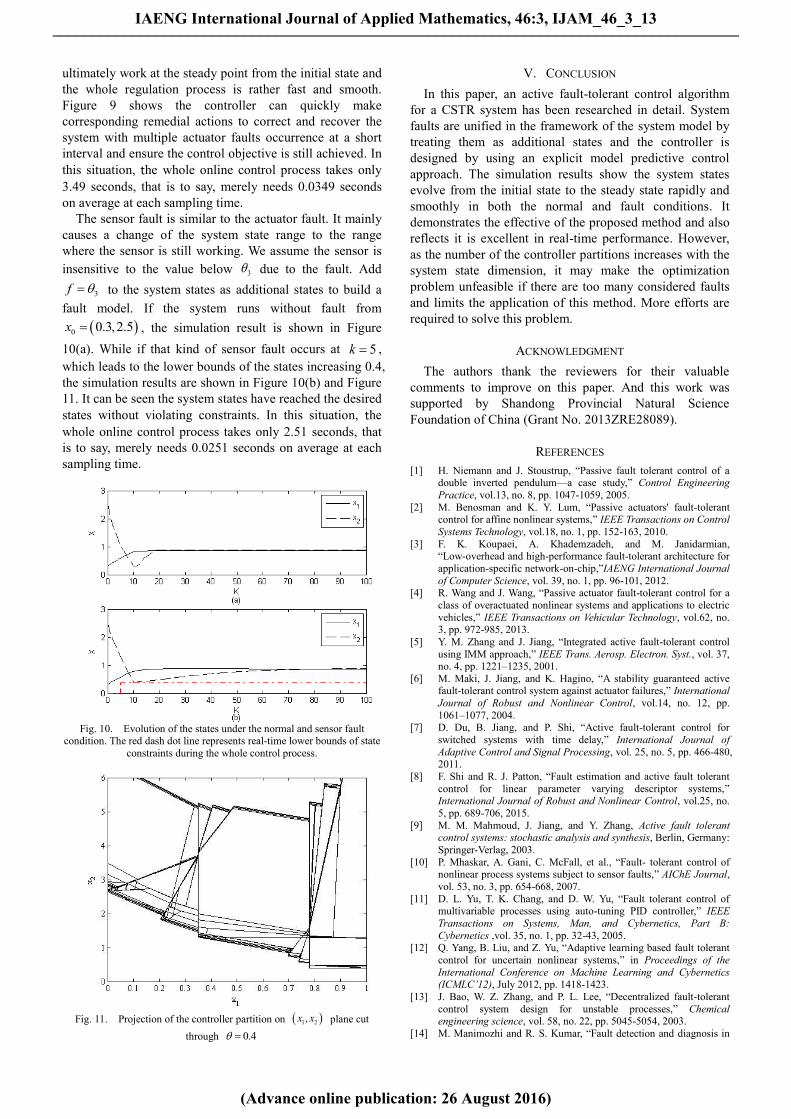
The sensor fault is similar to the actuator fault. It mainly

causes a change of the system state range to the range

where the sensor is still working. We assume the sensor is

insensitive to the value below 3 due to the fault. Add

3f to the system states as additional states to build a

fault model. If the system runs without fault from

0 0.3,2.5x , the simulation result is shown in Figure

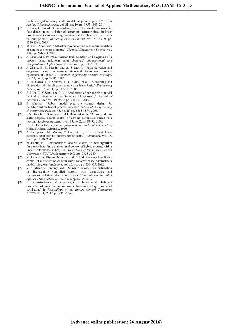
10(a). While if that kind of sensor fault occurs at 5k ,

which leads to the lower bounds of the states increasing 0.4,

the simulation results are shown in Figure 10(b) and Figure

11. It can be seen the system states have reached the desired

states without violating constraints. In this situation, the

whole online control process takes only 2.51 seconds, that

is to say, merely needs 0.0251 seconds on average at each

sampling time.

Fig. 10. Evolution of the states under the normal and sensor fault condition. The red dash dot line represents real-time lower bounds of state

constraints during the whole control process.


through 0.4

V. CONCLUSION

In this paper, an active fault-tolerant control algorithm

for a CSTR system has been researched in detail. System

faults are unified in the framework of the system model by

treating them as additional states and the controller is

designed by using an explicit model predictive control

approach. The simulation results show the system states

evolve from the initial state to the steady state rapidly and

smoothly in both the normal and fault conditions. It

demonstrates the effective of the proposed method and also

reflects it is excellent in real-time performance. However,

as the number of the controller partitions increases with the

system state dimension, it may make the optimization

problem unfeasible if there are too many considered faults

and limits the application of this method. More efforts are

required to solve this problem.

ACKNOWLEDGMENT

The authors thank the reviewers for their valuable

comments to improve on this paper. And this work was

supported by Shandong Provincial Natural Science

Foundation of China (Grant No. 2013ZRE28089).

REFERENCES

[1] H. Niemann and J. Stoustrup, ―Passive fault tolerant control of a double inverted pendulum—a case study,‖ Control Engineering

Practice, vol.13, no. 8, pp. 1047-1059, 2005.

[2] M. Benosman and K. Y. Lum, ―Passive actuators' fault-tolerant control for affine nonlinear systems,‖ IEEE Transactions on Control

Systems Technology, vol.18, no. 1, pp. 152-163, 2010.

[3] F. K. Koupaei, A. Khademzadeh, and M. Janidarmian, ―Low-overhead and high-performance fault-tolerant architecture for

application-specific network-on-chip,‖IAENG International Journal

of Computer Science, vol. 39, no. 1, pp. 96-101, 2012. [4] R. Wang and J. Wang, ―Passive actuator fault-tolerant control for a

class of overactuated nonlinear systems and applications to electric

vehicles,‖ IEEE Transactions on Vehicular Technology, vol.62, no. 3, pp. 972-985, 2013.

[5] Y. M. Zhang and J. Jiang, ―Integrated active fault-tolerant control

using IMM approach,‖ IEEE Trans. Aerosp. Electron. Syst., vol. 37, no. 4, pp. 1221–1235, 2001.

[6] M. Maki, J. Jiang, and K. Hagino, ―A stability guaranteed active fault-tolerant control system against actuator failures,‖ International

Journal of Robust and Nonlinear Control, vol.14, no. 12, pp.

1061–1077, 2004. [7] D. Du, B. Jiang, and P. Shi, ―Active fault-tolerant control for

switched systems with time delay,‖ International Journal of

Adaptive Control and Signal Processing, vol. 25, no. 5, pp. 466-480, 2011.

[8] F. Shi and R. J. Patton, ―Fault estimation and active fault tolerant

control for linear parameter varying descriptor systems,‖ International Journal of Robust and Nonlinear Control, vol.25, no.

5, pp. 689-706, 2015.

[9] M. M. Mahmoud, J. Jiang, and Y. Zhang, Active fault tolerant control systems: stochastic analysis and synthesis, Berlin, Germany:

Springer-Verlag, 2003.

[10] P. Mhaskar, A. Gani, C. McFall, et al., ―Fault- tolerant control of nonlinear process systems subject to sensor faults,‖ AIChE Journal,

vol. 53, no. 3, pp. 654-668, 2007.

[11] D. L. Yu, T. K. Chang, and D. W. Yu, ―Fault tolerant control of

multivariable processes using auto-tuning PID controller,‖ IEEE

Transactions on Systems, Man, and Cybernetics, Part B:

Cybernetics ,vol. 35, no. 1, pp. 32-43, 2005. [12] Q. Yang, B. Liu, and Z. Yu, ―Adaptive learning based fault tolerant

control for uncertain nonlinear systems,‖ in Proceedings of the

International Conference on Machine Learning and Cybernetics (ICMLC’12), July 2012, pp. 1418-1423.

[13] J. Bao, W. Z. Zhang, and P. L. Lee, ―Decentralized fault-tolerant

control system design for unstable processes,‖ Chemical engineering science, vol. 58, no. 22, pp. 5045-5054, 2003.

[14] M. Manimozhi and R. S. Kumar, ―Fault detection and diagnosis in



______________________________________________________________________________________

nonlinear system using multi model adaptive approach,‖ World

Applied Sciences Journal, vol. 31, no. 10, pp. 1857-1863, 2014.

[15] F. Kiasi, J. Prakash, S. Patwardhan, et al., ―A unified framework for

fault detection and isolation of sensor and actuator biases in linear

time invariant systems using marginalized likelihood ratio test with

uniform priors,‖ Journal of Process Control, vol. 23, no. 9, pp. 1350-1361, 2013.

[16] M. Du, J. Scott, and P. Mhaskar, ―Actuator and sensor fault isolation

of nonlinear process systems,‖ Chemical Engineering Science, vol. 104, pp. 294-303, 2013.

[17] J. Zarei and J. Poshtan, ―Sensor fault detection and diagnosis of a

process using unknown input observer,‖ Mathematical and Computational Applications, vol. 16, no. 1, pp. 31–41, 2011.

[18] J. Zhang, E. B. Martin, and A. J. Morris. ―Fault detection and

diagnosis using multivariate statistical techniques: Process operations and control,‖ Chemical engineering research & design,

vol. 74, no. 1, pp. 89-96, 1996.

[19] A. A. Garza, J. J. Serrano, R. O. Carot, et al., ―Monitoring and diagnostics with intelligent agents using fuzzy logic,‖ Engineering

Letters, vol. 15, no. 1, pp. 105-111, 2007.

[20] J. J. Du, C. Y. Song, and P. Li, ―Application of gap metric to model bank determination in multilinear model approach,‖ Journal of

Process Control, vol. 19, no. 2, pp. 231-240, 2009.

[21] P. Mhaskar, ―Robust model predictive control design for fault-tolerant control of process systems,‖ Industrial & engineering

chemistry research, vol. 45, no. 25, pp. 8565-8574, 2006.

[22] I. S. Baruch, P. Georgieva, and J. Barrera-Cortés, ―An integral plus states adaptive neural control of aerobic continuous stirred tank

reactor,‖ Engineering Letters, vol. 13, no. 2, pp. 84-92, 2006.

[23] D. P. Bertsekas, Dynamic programming and optimal control, Nashua: Athena Scientific, 1996.

[24] A. Bemporad, M. Morari, V. Dua, et al., ―The explicit linear

quadratic regulator for constrained systems,‖ Automatica, vol. 38, no. 1, pp. 3-20, 2002.

[25] M. Baotic, F. J. Christophersen, and M. Morari, ―A new algorithm

for constrained finite time optimal control of hybrid systems with a

linear performance index,‖ in Proceedings of the Europe Control

Conference (ECC’03), September 2003, pp. 3335-3340.

[26] K. Ramesh, A. Hisyam, N. Aziz, et al., ―Nonlinear model predictive control of a distillation column using wavenet based hammerstein

model,‖ Engineering Letters, vol. 20, no.4, pp. 330-335, 2012. [27] V. Y. Glizer, V. Turetsky, and J. Shinar, ―Terminal cost distribution

in discrete-time controlled system with disturbance and

noise-corrupted state information,‖ IAENG International Journal of Applied Mathematics, vol. 42, no. 1, pp. 52-59, 2012

[28] F. J. Christophersen, M. Kvasnica, C. N. Jones, et al., ―Efficient

evaluation of piecewise control laws defined over a large number of polyhedra,‖ in Proceedings of the Europe Control Conference

(ECC’07), July 2007, pp. 2360-2367.



______________________________________________________________________________________

active fault-tolerant control of a cstr system based on ... · therefore is widely used in the...

Documents