active learning and optimized information...
TRANSCRIPT

Active Learning and
Optimized Information Gathering
Lecture 12 – Submodularity
CS 101.2
Andreas Krause

2
AnnouncementsHomework 2: Due Thursday Feb 19
Project milestone due: Feb 24
4 Pages, NIPS format:
http://nips.cc/PaperInformation/StyleFiles
Should contain preliminary results (model, experiments,
proofs, …) as well as timeline for remaining work
Come to office hours to discuss projects!
Office hours
Come to office hours before your presentation!
Andreas: Monday 3pm-4:30pm, 260 Jorgensen
Ryan: Wednesday 4:00-6:00pm, 109 Moore

3
Course outline1. Online decision making
2. Statistical active learning
3. Combinatorial approaches
4
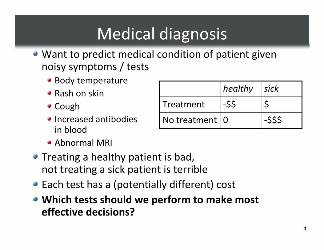
Medical diagnosisWant to predict medical condition of patient given noisy symptoms / tests
Body temperature
Rash on skin
Cough
Increased antibodies in blood
Abnormal MRI
Treating a healthy patient is bad, not treating a sick patient is terrible
Each test has a (potentially different) cost
Which tests should we perform to make most effective decisions?
-$$$0No treatment
$-$$Treatment
sickhealthy
5
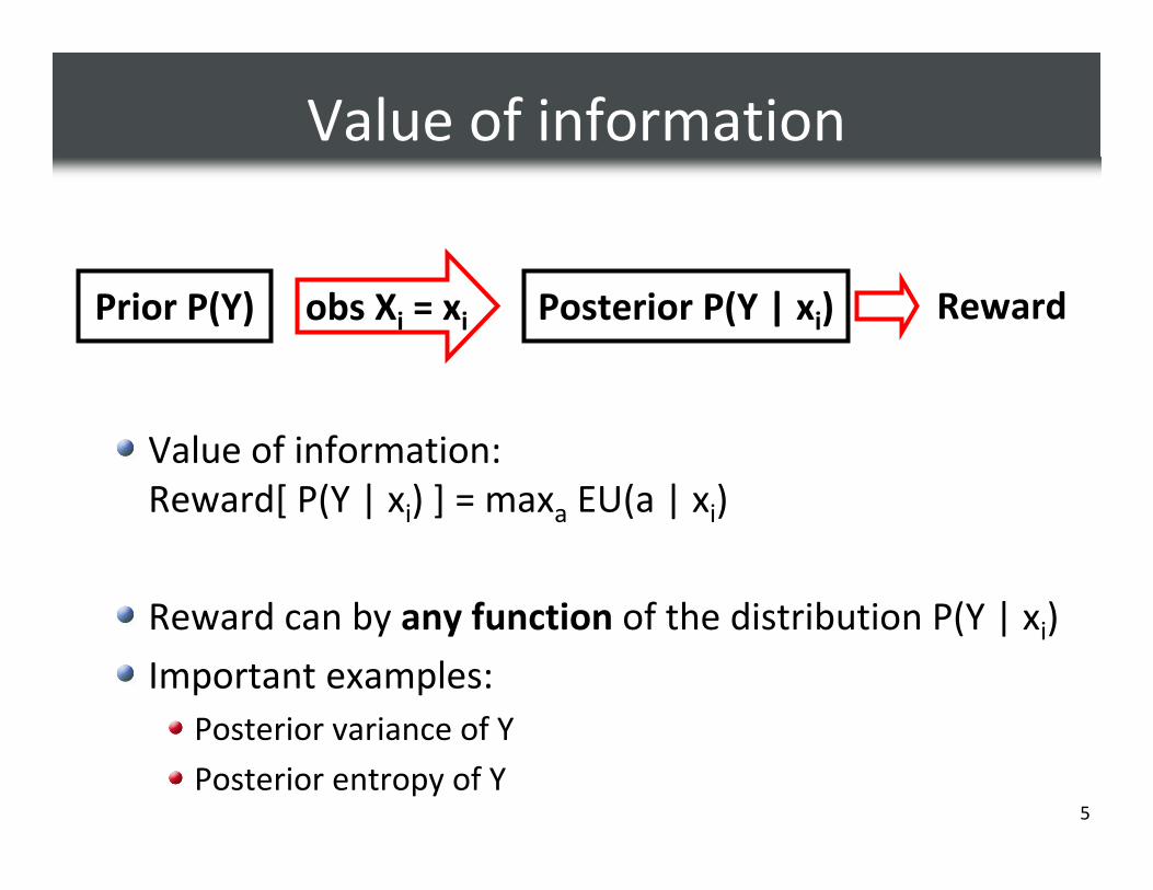
Value of information
Value of information:
Reward[ P(Y | xi) ] = maxa EU(a | xi)
Reward can by any function of the distribution P(Y | xi)
Important examples:
Posterior variance of Y
Posterior entropy of Y
Prior P(Y) Posterior P(Y | xi)obs Xi = xi Reward

6
Optimal value of informationCan we efficiently optimize value of information?
� Answer depends on properties of the distribution P(X1,…,Xn,Y)
Theorem [Krause & Guestrin IJCAI ’05]:
If the random variables form a Markov Chain, can find optimal (exponentially large!) decision tree in polynomial time ☺
There exists a class of distributions for which we can perform efficient inference (i.e., compute P(Y|Xi)), where finding the optimal decision tree is NPPP hard

7
Approximating value of information?If we can’t find an optimal solution, can we find
provably near-optimal approximations??
8
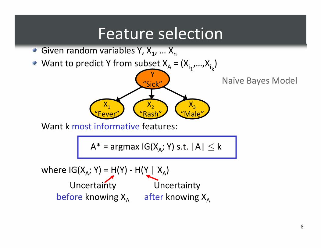
Feature selectionGiven random variables Y, X1, … Xn
Want to predict Y from subset XA = (Xi1,…,Xik
)
Want k most informative features:
A* = argmax IG(XA; Y) s.t. |A| ≤ k
where IG(XA; Y) = H(Y) - H(Y | XA)
Y
“Sick”
X1
“Fever”
X2
“Rash”
X3
“Male”
Naïve Bayes Model
Uncertainty
before knowing XA
Uncertainty
after knowing XA
9
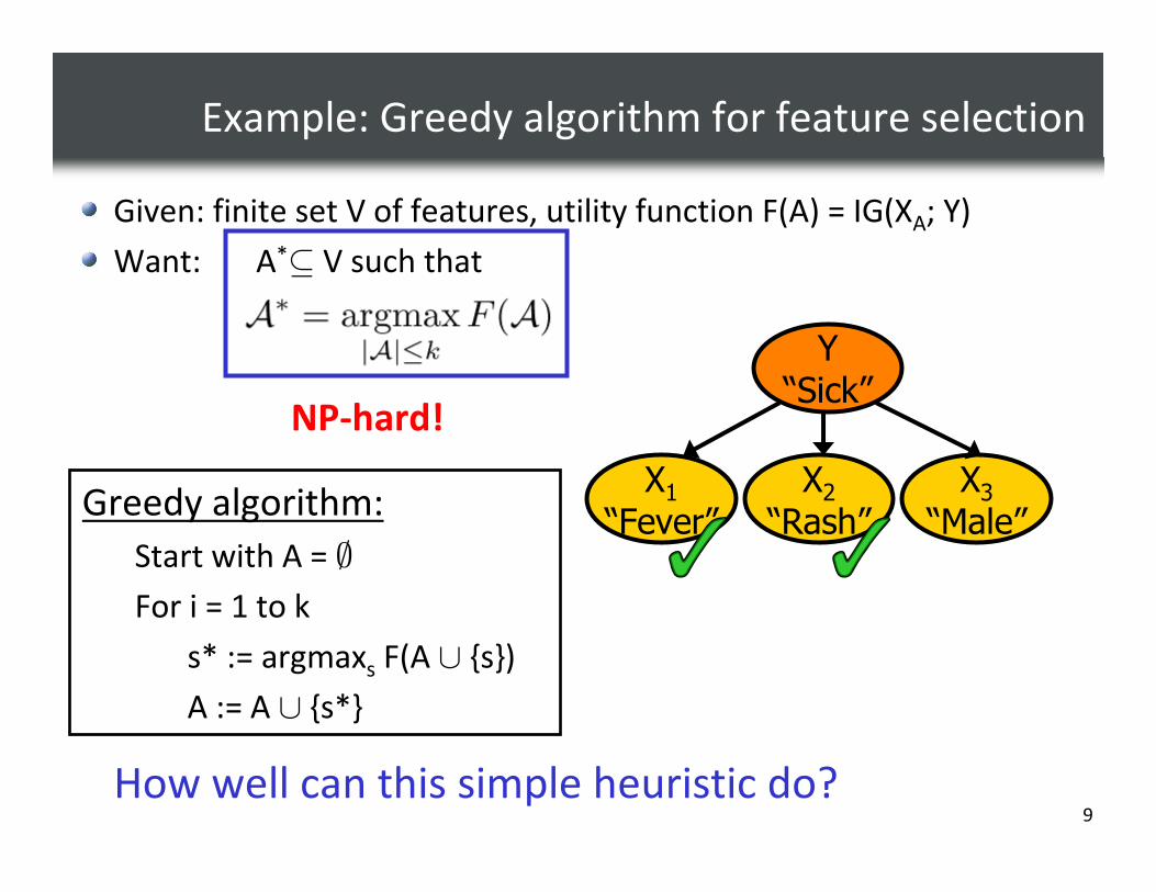
Example: Greedy algorithm for feature selection
Given: finite set V of features, utility function F(A) = IG(XA; Y)
Want: A*⊆ V such that
NP-hard!
How well can this simple heuristic do?
Greedy algorithm:
Start with A = ∅
For i = 1 to k
s* := argmaxs F(A ∪ {s})
A := A ∪ {s*}
Y“Sick”
X1“Fever”
X2“Rash”
X3“Male”
10
s
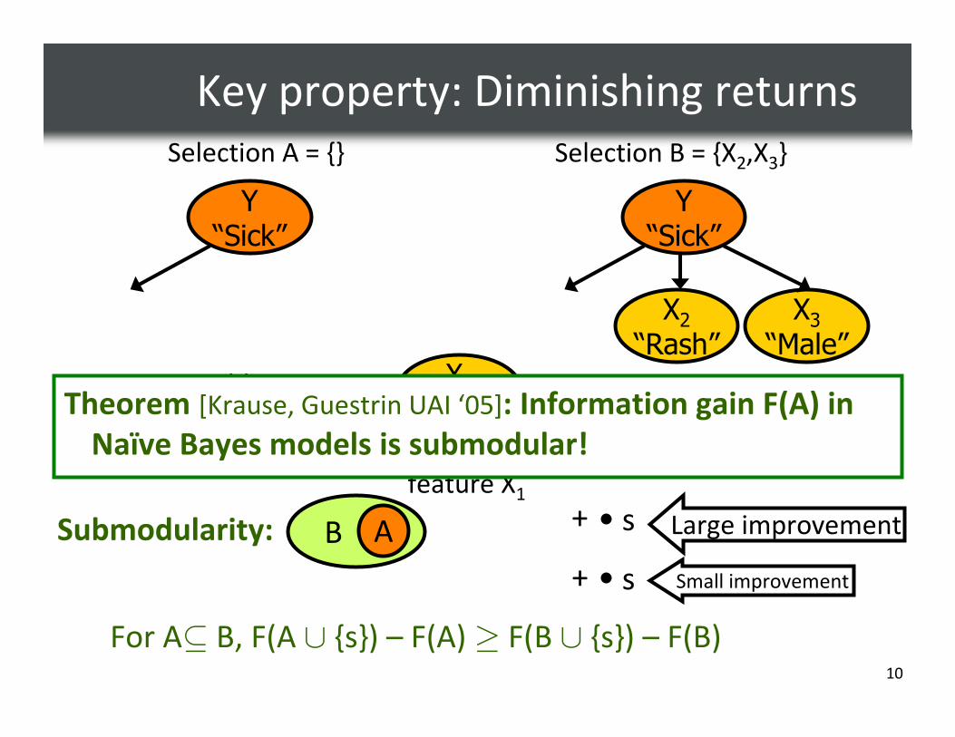
Key property: Diminishing returns
Selection A = {} Selection B = {X2,X3}
Adding X1
will help a lot!Adding X1
doesn’t help muchNew
feature X1
B A
s
+
+
Large improvement
Small improvement
For A⊆ B, F(A ∪ {s}) – F(A) ≥ F(B ∪ {s}) – F(B)
Submodularity:
Y“Sick”
X1“Fever”
X2“Rash”
X3“Male”
Y“Sick”
Theorem [Krause, Guestrin UAI ‘05]: Information gain F(A) in
Naïve Bayes models is submodular!

11
Why is submodularity useful?
Theorem [Nemhauser et al ‘78]
Greedy maximization algorithm returns Agreedy:
F(Agreedy) ≥ (1-1/e) max|A|≤ k F(A)
Greedy algorithm gives near-optimal solution!
For info-gain: Guarantees best possible unless P = NP!
[Krause, Guestrin UAI ’05]
Submodularity is an incredibly useful and powerful concept!
~63%
12
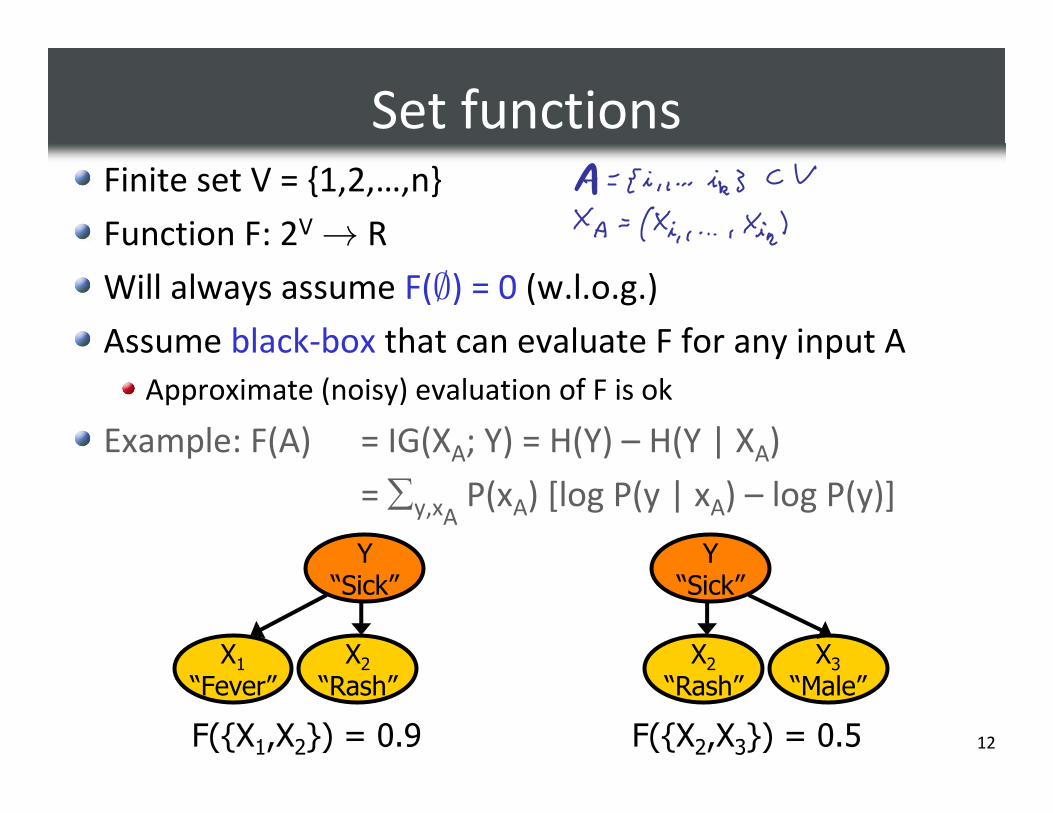
Set functionsFinite set V = {1,2,…,n}
Function F: 2V → R
Will always assume F(∅) = 0 (w.l.o.g.)
Assume black-box that can evaluate F for any input A
Approximate (noisy) evaluation of F is ok
Example: F(A) = IG(XA; Y) = H(Y) – H(Y | XA)
= ∑y,xAP(xA) [log P(y | xA) – log P(y)]
Y“Sick”
X1
“Fever”X2
“Rash”
F({X1,X2}) = 0.9
Y“Sick”
X2
“Rash”X3
“Male”
F({X2,X3}) = 0.5
13
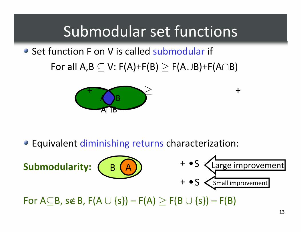
Submodular set functionsSet function F on V is called submodular if
For all A,B ⊆ V: F(A)+F(B) ≥ F(A∪B)+F(A�B)
Equivalent diminishing returns characterization:
SB A
S
+
+
Large improvement
Small improvement
For A⊆B, s∉B, F(A ∪ {s}) – F(A) ≥ F(B ∪ {s}) – F(B)
Submodularity:
BA A ∪ B
A�B
++ ≥
14
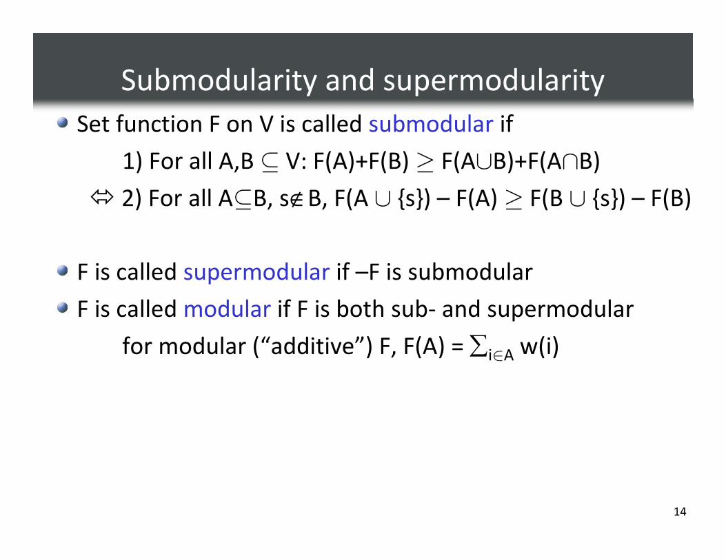
Submodularity and supermodularity
Set function F on V is called submodular if
1) For all A,B ⊆ V: F(A)+F(B) ≥ F(A∪B)+F(A�B)
� 2) For all A⊆B, s∉B, F(A ∪ {s}) – F(A) ≥ F(B ∪ {s}) – F(B)
F is called supermodular if –F is submodular
F is called modular if F is both sub- and supermodular
for modular (“additive”) F, F(A) = ∑i∈A w(i)

15
Example: Set cover
Node predicts
values of positions
with some radius
SERVER
LAB
KITCHEN
COPYELEC
PHONEQUIET
STORAGE
CONFERENCE
OFFICEOFFICE
For A ⊆ V: F(A) = “area
covered by sensors placed at A”
Formally:
W finite set, collection of n subsets Si ⊆W
For A ⊆ V={1,…,n} define F(A) = |Ui∈ A Si|
Want to cover floorplan with discsPlace sensorsin building Possible
locations V

16
Set cover is submodular
SERVER
LAB
KITCHEN
COPYELEC
PHONEQUIET
STORAGE
CONFERENCE
OFFICEOFFICE
SERVER
LAB
KITCHEN
COPYELEC
PHONEQUIET
STORAGE
CONFERENCE
OFFICEOFFICE
S1 S2
S1 S2
S3
S4 S’
S’
A={S1,S2}
B = {S1,S2,S3,S4}
F(A∪{S’})-F(A)
F(B∪{S’})-F(B)
≥
17
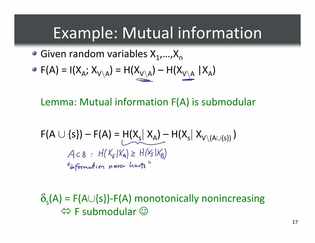
Example: Mutual informationGiven random variables X1,…,Xn
F(A) = I(XA; XV\A) = H(XV\A) – H(XV\A |XA)
Lemma: Mutual information F(A) is submodular
F(A ∪ {s}) – F(A) = H(Xs| XA) – H(Xs| XV\(A∪{s}) )
δs(A) = F(A∪{s})-F(A) monotonically nonincreasing
� F submodular ☺
18
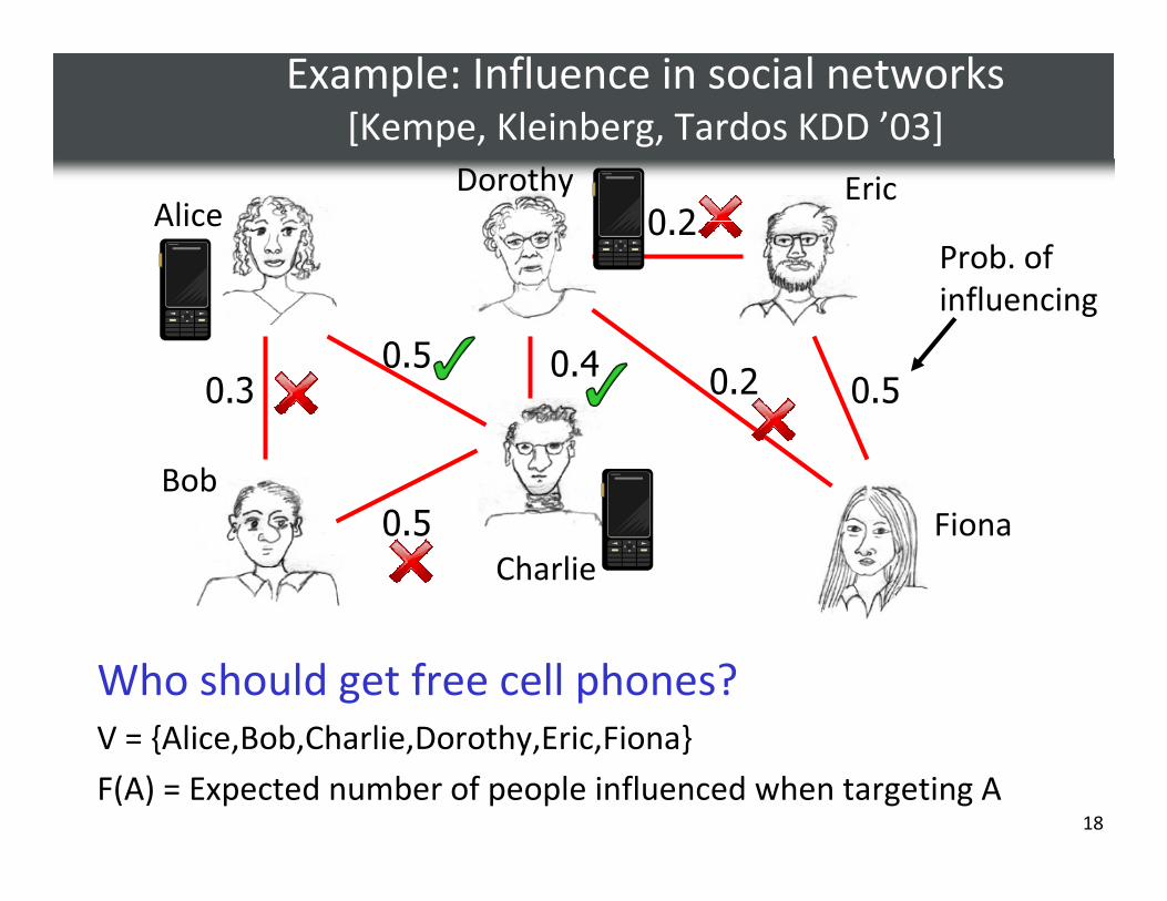
Example: Influence in social networks[Kempe, Kleinberg, Tardos KDD ’03]
Who should get free cell phones?V = {Alice,Bob,Charlie,Dorothy,Eric,Fiona}
F(A) = Expected number of people influenced when targeting A
0.5
0.30.5 0.4
0.2
0.2 0.5
Alice
Bob
Charlie
Dorothy Eric
Fiona
Prob. of
influencing

19
Influence in social networks is submodular[Kempe, Kleinberg, Tardos KDD ’03]
0.5
0.30.5 0.4
0.2
0.2 0.5
Alice
Bob
Charlie
Dorothy Eric
Fiona
Key idea: Flip coins c in advance � “live” edges
Fc(A) = People influenced under outcome c (set cover!)
F(A) = ∑c P(c) Fc(A) is submodular as well!
20
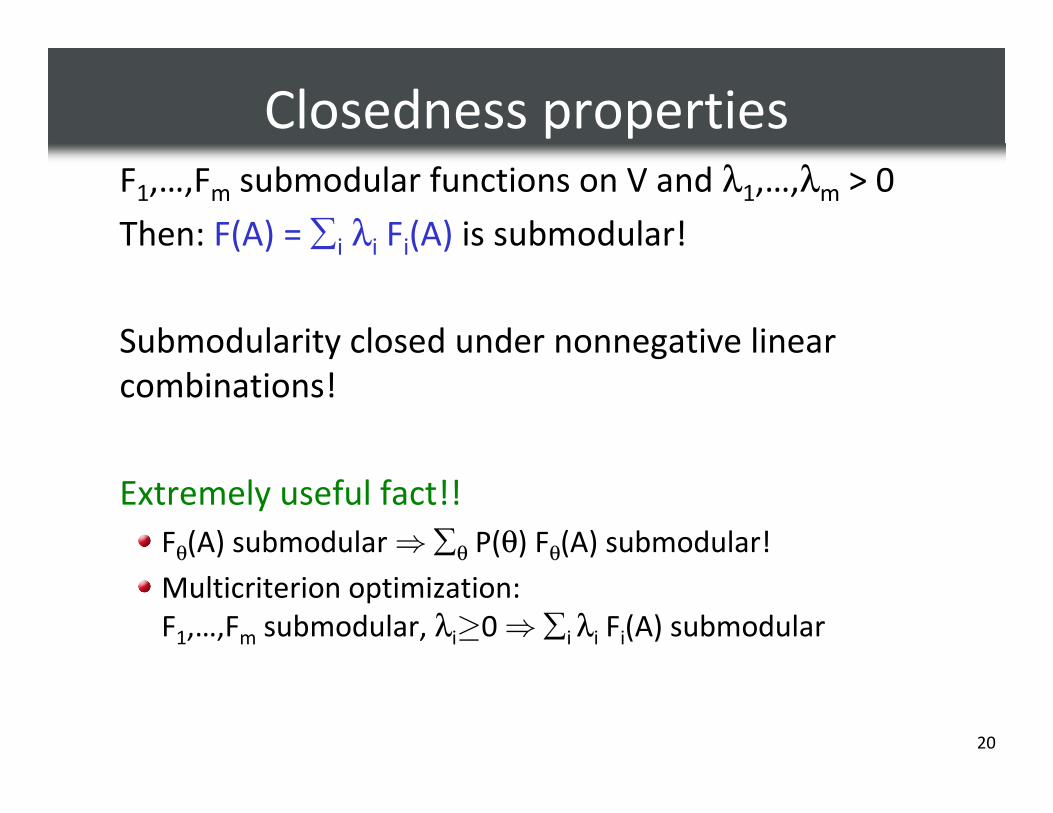
Closedness propertiesF1,…,Fm submodular functions on V and λ1,…,λm > 0
Then: F(A) = ∑i λi Fi(A) is submodular!
Submodularity closed under nonnegative linear
combinations!
Extremely useful fact!!
Fθ(A) submodular ⇒ ∑θ P(θ) Fθ(A) submodular!
Multicriterion optimization:
F1,…,Fm submodular, λi≥0 ⇒ ∑i λi Fi(A) submodular

21
Submodularity and ConcavitySuppose g: N → R and F(A) = g(|A|)
Then F(A) submodular if and only if g concave!
E.g., g could say “buying in bulk is cheaper”
|A|
g(|A|)

22
Maximum of submodular functions
Suppose F1(A) and F2(A) submodular.
Is F(A) = max(F1(A),F2(A)) submodular?
|A|
F2(A)
F1(A)
F(A) = max(F1(A),F2(A))
max(F1,F2) not submodular in general!

23
Minimum of submodular functions
Well, maybe F(A) = min(F1(A),F2(A)) instead?
111{a,b}
010{b}
001{a}
000∅
F(A)F2(A)F1(A)F({b}) – F(∅)=0
F({a,b}) – F({a})=1
<
But stay tuned – we’ll address mini Fi later!
min(F1,F2) not submodular in general!
24
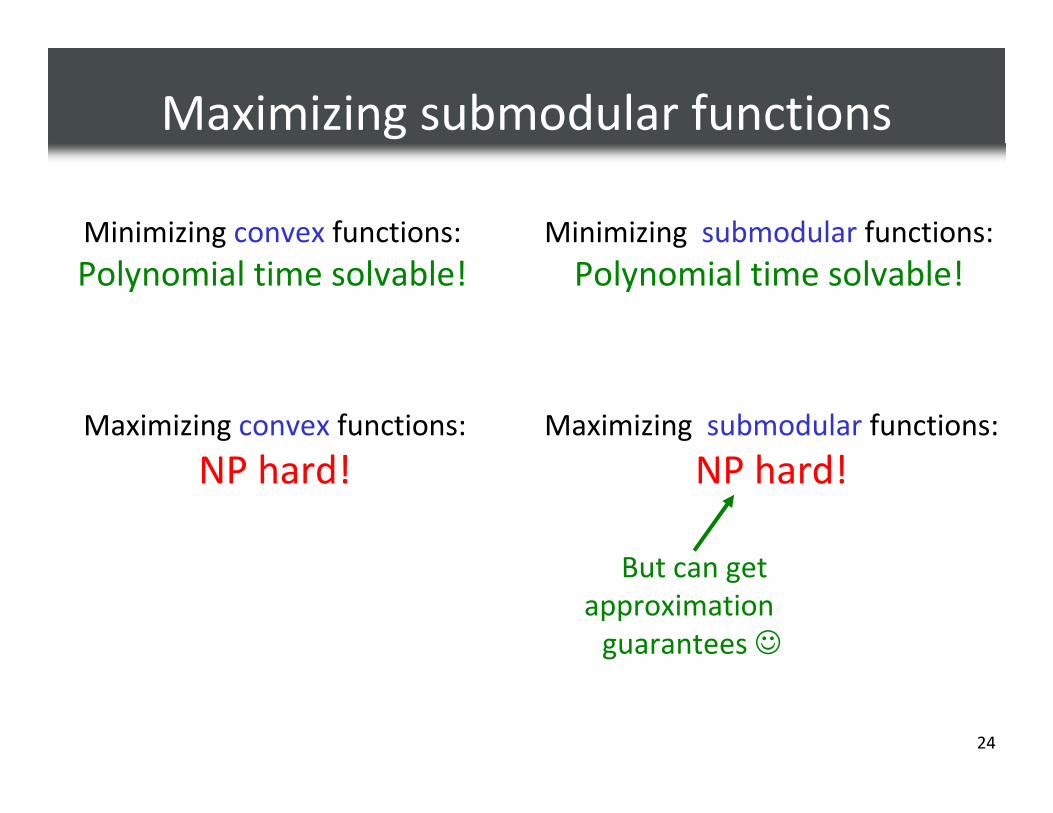
Maximizing submodular functions
Minimizing convex functions:
Polynomial time solvable!
Minimizing submodular functions:
Polynomial time solvable!
Maximizing convex functions:
NP hard!Maximizing submodular functions:
NP hard!
But can get
approximation
guarantees ☺

25
Maximizing influence[Kempe, Kleinberg, Tardos KDD ’03]
F(A) = Expected #people influenced when targeting A
F monotonic: If A ⊆ B: F(A) ≤ F(B) Hence V = argmaxA F(A)
More interesting: argmaxA F(A) – Cost(A)
0.5
0.30.5 0.4
0.2
0.2 0.5
Alice
Bob
Charlie
Eric
Fiona
Dorothy
26
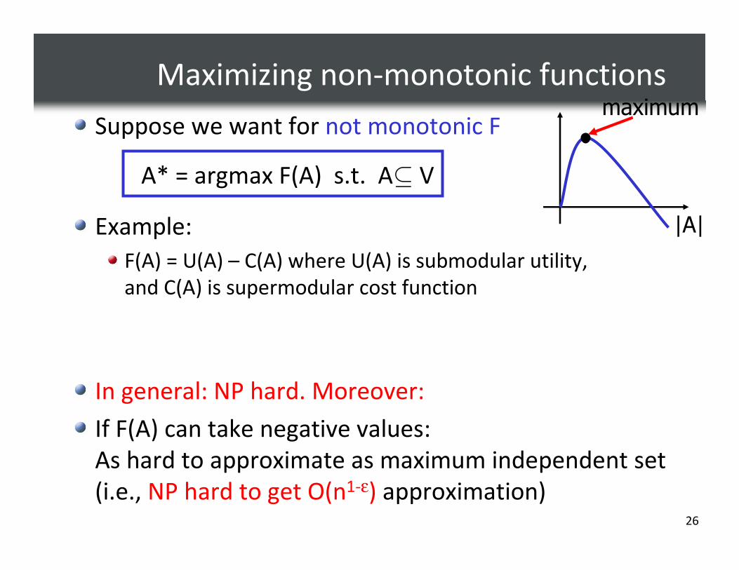
Maximizing non-monotonic functions
Suppose we want for not monotonic F
A* = argmax F(A) s.t. A⊆ V
Example:
F(A) = U(A) – C(A) where U(A) is submodular utility,
and C(A) is supermodular cost function
In general: NP hard. Moreover:
If F(A) can take negative values:
As hard to approximate as maximum independent set
(i.e., NP hard to get O(n1-ε) approximation)
|A|
maximum

27
Maximizing positive submodular functions[Feige, Mirrokni, Vondrak FOCS ’07]
picking a random set gives ¼ approximation
(½ approximation if F is symmetric!)
we cannot get better than ¾ approximation unless P = NP
Theorem
There is an efficient randomized local search procedure,
that, given a positive submodular function F, F(∅)=0,
returns set ALS such that
F(ALS) ≥ (2/5) maxA F(A)
28
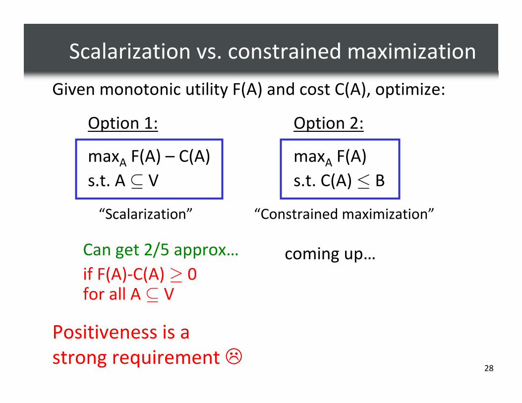
Scalarization vs. constrained maximization
Given monotonic utility F(A) and cost C(A), optimize:
Option 1:
maxA F(A) – C(A)
s.t. A ⊆ V
Option 2:
maxA F(A)
s.t. C(A) ≤ B
Can get 2/5 approx…
if F(A)-C(A) ≥ 0 for all A ⊆ V
coming up…
Positiveness is a
strong requirement �
“Scalarization” “Constrained maximization”

29
Robust optimization Complex constraints
Constrained maximization: Outline
Selected setMonotonic submodular
BudgetSelection cost
Subset selection: C(A) = |A|
30
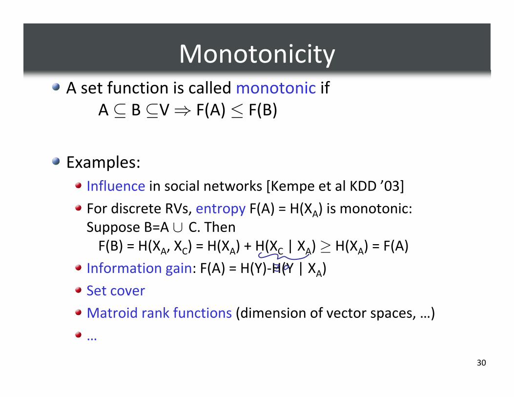
MonotonicityA set function is called monotonic if
A ⊆ B ⊆V ⇒ F(A) ≤ F(B)
Examples:
Influence in social networks [Kempe et al KDD ’03]
For discrete RVs, entropy F(A) = H(XA) is monotonic:
Suppose B=A ∪ C. Then
F(B) = H(XA, XC) = H(XA) + H(XC | XA) ≥ H(XA) = F(A)
Information gain: F(A) = H(Y)-H(Y | XA)
Set cover
Matroid rank functions (dimension of vector spaces, …)
…
31
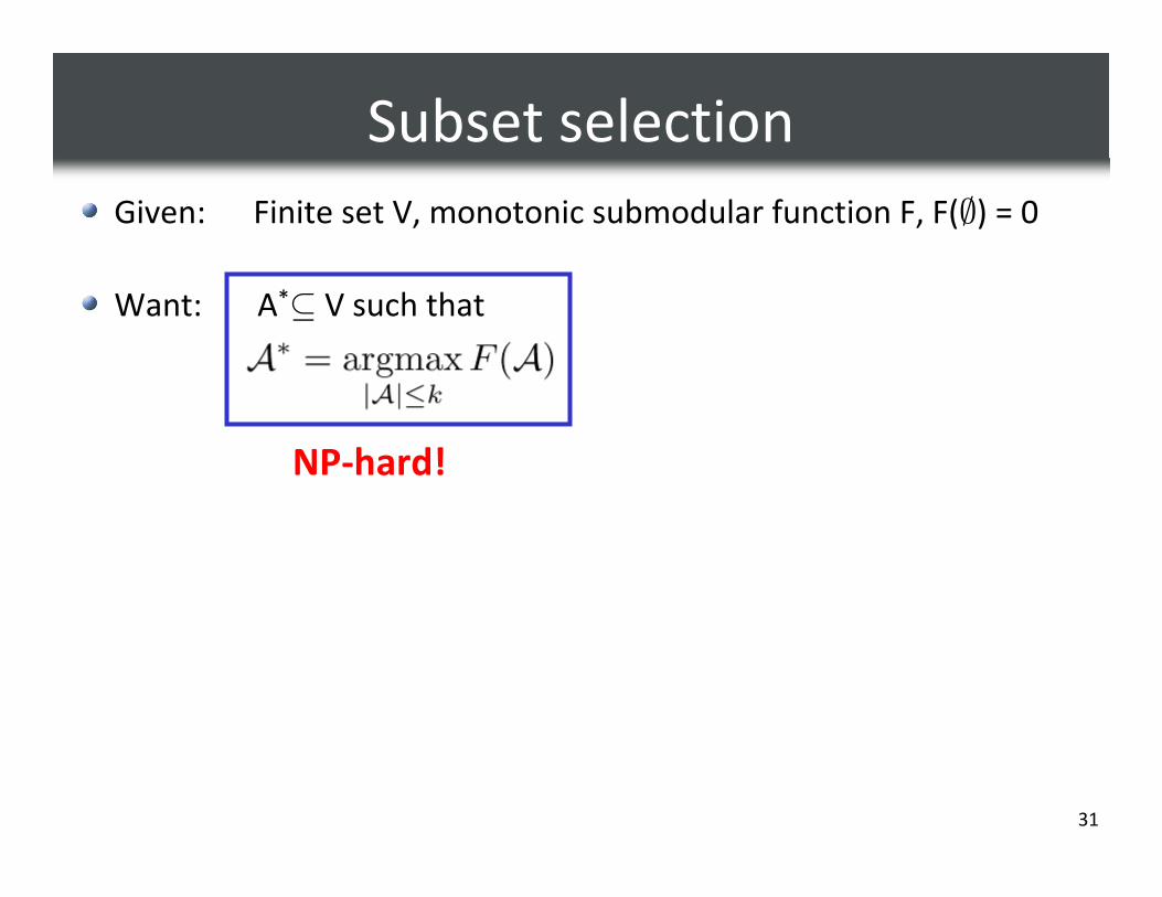
Subset selection
Given: Finite set V, monotonic submodular function F, F(∅) = 0
Want: A*⊆ V such that
NP-hard!
32
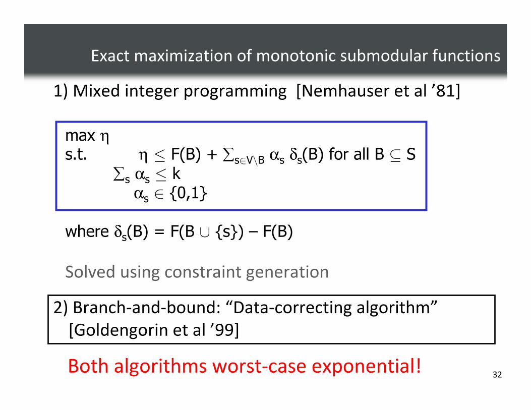
Exact maximization of monotonic submodular functions
1) Mixed integer programming [Nemhauser et al ’81]
2) Branch-and-bound: “Data-correcting algorithm”
[Goldengorin et al ’99]
max ηs.t. η ≤ F(B) + ∑s∈V\B αs δs(B) for all B ⊆ S
∑s αs ≤ kαs ∈ {0,1}
where δs(B) = F(B ∪ {s}) – F(B)
Solved using constraint generation
Both algorithms worst-case exponential!
33
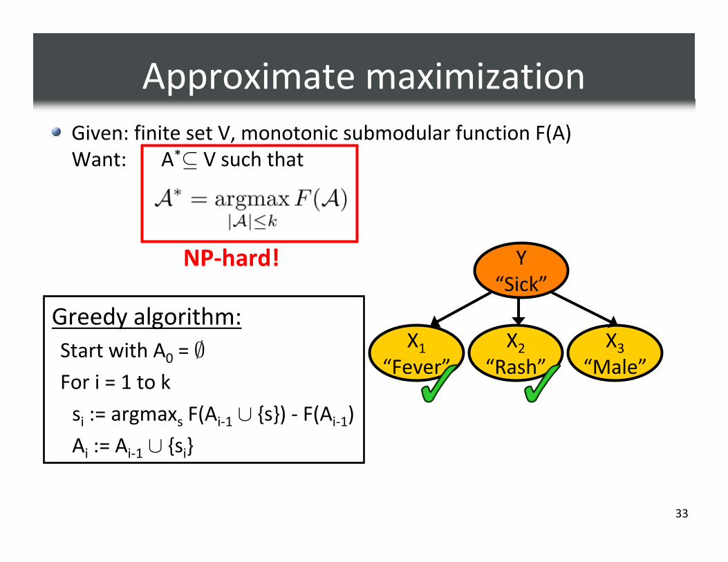
Approximate maximization
Given: finite set V, monotonic submodular function F(A)
Want: A*⊆ V such that
NP-hard!
Greedy algorithm:
Start with A0 = ∅
For i = 1 to k
si := argmaxs F(Ai-1 ∪ {s}) - F(Ai-1)
Ai := Ai-1 ∪ {si}
Y
“Sick”
X1
“Fever”
X2
“Rash”
X3
“Male”

34
Performance of greedy algorithm
Theorem [Nemhauser et al ‘78]
Given a monotonic submodular function F, F(∅)=0, the
greedy maximization algorithm returns Agreedy
F(Agreedy) ≥ (1-1/e) max|A|· k F(A)
~63%
Sidenote: Greedy algorithm gives 1/2 approximation for maximization over any matroid C! [Fisher et al ’78]
35
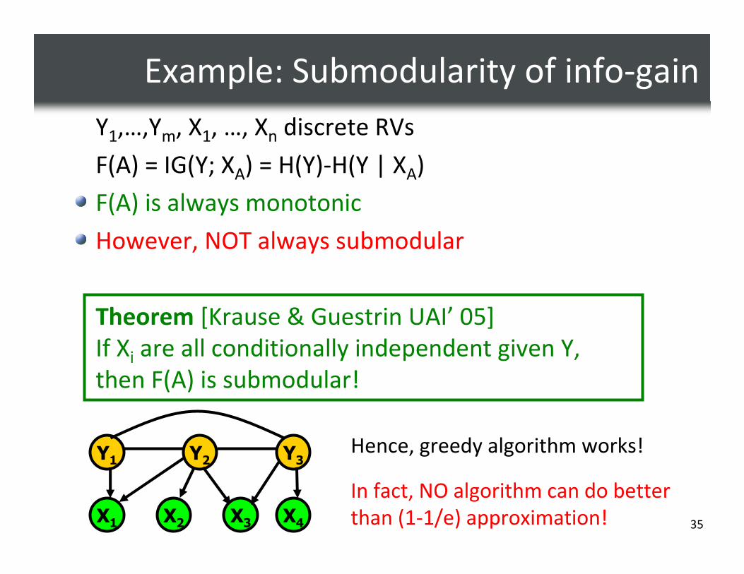
Example: Submodularity of info-gain
Y1,…,Ym, X1, …, Xn discrete RVs
F(A) = IG(Y; XA) = H(Y)-H(Y | XA)
F(A) is always monotonic
However, NOT always submodular
Theorem [Krause & Guestrin UAI’ 05]
If Xi are all conditionally independent given Y,
then F(A) is submodular!
Y1
X1
Y2
X2
Y3
X4
X3
Hence, greedy algorithm works!
In fact, NO algorithm can do better
than (1-1/e) approximation!

36
People sit a lot
Activity recognition in
assistive technologies
Seating pressure as
user interface
Equipped with
1 sensor per cm2!
Costs $16,000! �
Can we get similar
accuracy with fewer,
cheaper sensors?
Lean
forward
SlouchLean
left
82% accuracy on
10 postures! [Tan et al]
Building a Sensing Chair [Mutlu, Krause, Forlizzi, Guestrin, Hodgins UIST ‘07]

37
How to place sensors on a chair?
Sensor readings at locations V as random variables
Predict posture Y using probabilistic model P(Y,V)
Pick sensor locations A* ⊆ V to minimize entropy:
Possible locations V
$100 ☺☺☺☺79%After
$16,000 ����82%Before
CostAccuracy
Placed sensors, did a user study:
Similar accuracy at <1% of the cost!

38
Variance reduction (a.k.a. Orthogonal matching pursuit, Forward Regression)
Let Y = ∑i αi Xi+ε, and (X1,…,Xn,ε) ∼ N(·; µ,Σ)
Want to pick subset XA to predict Y
Var(Y | XA=xA): conditional variance of Y given XA = xA
Expected variance: Var(Y | XA) = ∫ p(xA) Var(Y | XA=xA) dxA
Variance reduction: FV(A) = Var(Y) – Var(Y | XA)
FV(A) is always monotonic
Theorem [Das & Kempe, STOC ’08]
FV(A) is submodular**under some
conditions on Σ
���� Orthogonal matching pursuit near optimal!
[see other analyses by Tropp, Donoho et al., and Temlyakov]

39
Monitoring water networks[Krause et al, J Wat Res Mgt 2008]
Contamination of drinking water
could affect millions of people
Contamination
Place sensors to detect contaminations
“Battle of the Water Sensor Networks” competition
Where should we place sensors to quickly detect contamination?
Sensors
Simulator from EPA Hach Sensor
~$14K

40
Model-based sensing
Utility of placing sensors based on model of the world
For water networks: Water flow simulator from EPA
F(A)=Expected impact reduction placing sensors at A
S2
S3
S4S1 S2
S3
S4
S1
High impact reduction F(A) = 0.9 Low impact reduction F(A)=0.01
Model predicts
High impact
Medium impact
location
Low impact
location
Sensor reduces
impact through
early detection!
S1
Contamination
Set V of all
network junctions
Theorem [Krause et al., J Wat Res Mgt ’08]:
Impact reduction F(A) in water networks is submodular!
41
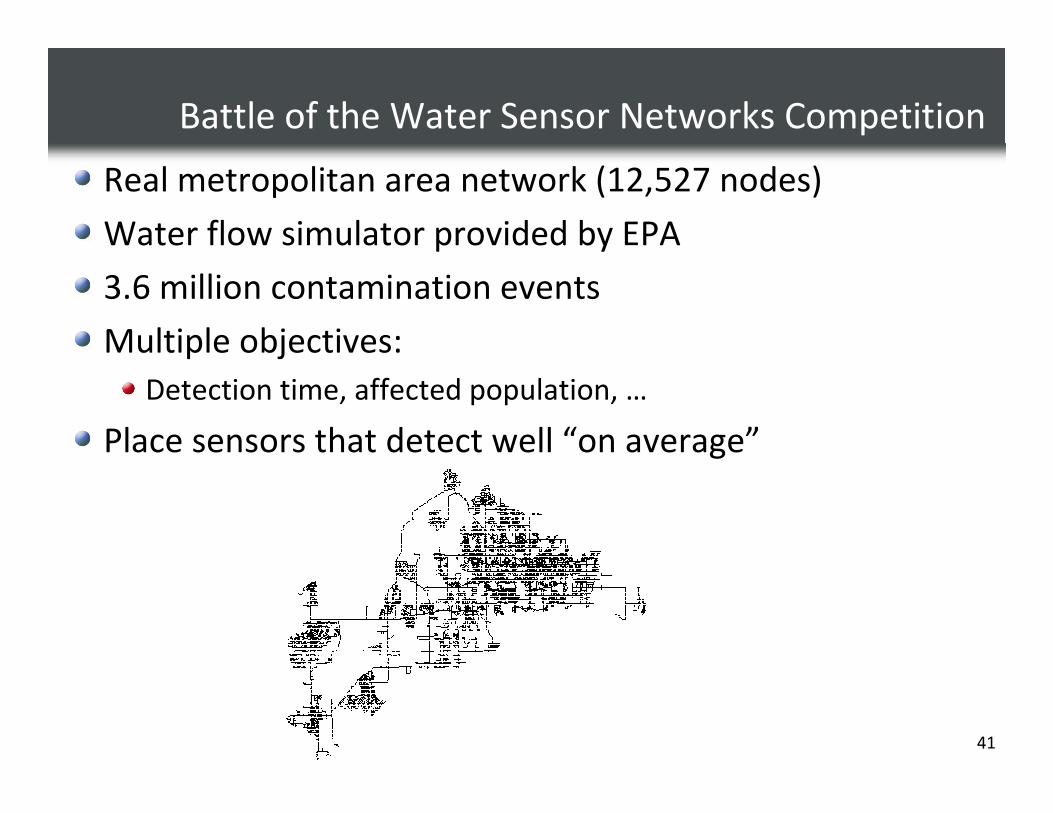
Battle of the Water Sensor Networks Competition
Real metropolitan area network (12,527 nodes)
Water flow simulator provided by EPA
3.6 million contamination events
Multiple objectives:
Detection time, affected population, …
Place sensors that detect well “on average”

42
Bounds on optimal solution[Krause et al., J Wat Res Mgt ’08]
(1-1/e) bound quite loose… can we get better bounds?
Po
pu
lati
on
pro
tect
ed
F(A
)
Hig
he
r is
be
tte
r
Water
networks
data
0 5 10 15 200
0.2
0.4
0.6
0.8
1
1.2
1.4Offline
(Nemhauser)
bound
Greedy
solution
Number of sensors placed
43
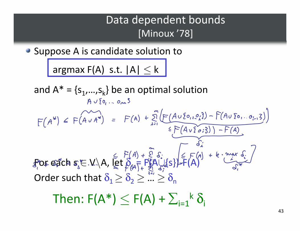
Data dependent bounds[Minoux ’78]
Suppose A is candidate solution to
argmax F(A) s.t. |A| ≤ k
and A* = {s1,…,sk} be an optimal solution
For each s ∈ V\A, let δs = F(A∪{s})-F(A)
Order such that δ1 ≥ δ2 ≥ …≥ δn
Then: F(A*) ≤ F(A) + ∑i=1k δi

44
Bounds on optimal solution[Krause et al., J Wat Res Mgt ’08]
Submodularity gives data-dependent bounds on the
performance of any algorithm
Sensing quality F(A)
Higher is better
Water
networks
data
0 5 10 15 200
0.2
0.4
0.6
0.8
1
1.2
1.4Offline
(Nemhauser)
bound Data-dependent
bound
Greedy
solution
Number of sensors placed

45
BWSN Competition results [Ostfeld et al., J Wat Res Mgt 2008]
13 participants
Performance measured in 30 different criteria
0
5
10
15
20
25
30
Total Score
Higher is better
Krause et al.
Berry et al.
Dorini et al.
Wu & Walski
Ostfeld& Salomons
Propato& Piller
Eliades& Polycarpou
Huang et al.
Guan et al.
Ghimire& Barkdoll
Trachtman
Gueli
Preis& Ostfeld
E
E
D DG
GG
GG
H
H
H
G: Genetic algorithm
H: Other heuristic
D: Domain knowledge
E: “Exact” method (MIP)
24% better performance than runner-up! ☺☺☺☺
46
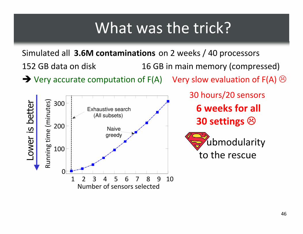
Simulated all on 2 weeks / 40 processors
152 GB data on disk
� Very accurate computation of F(A)
16 GB in main memory (compressed)
Lower is better
30 hours/20 sensors
6 weeks for all
30 settings ����
3.6M contaminations
Very slow evaluation of F(A) �
1 2 3 4 5 6 7 8 9 100
100
200
300
Number of sensors selected
Ru
nn
ing
tim
e (
min
ute
s)
Exhaustive search(All subsets)
Naivegreedy
What was the trick?
ubmodularity
to the rescue

47
Scaling up greedy algorithm[Minoux ’78]
In round i+1,
have picked Ai = {s1,…,si}
pick si+1 = argmaxs F(Ai ∪ {s})-F(Ai)
I.e., maximize “marginal benefit” δs(Ai)
δs(Ai) = F(Ai ∪ {s})-F(Ai)
Key observation: Submodularity implies
i ≤ j ⇒ δs(Ai) ≥ δs(Aj)
Marginal benefits can never increase!
s
δδδδs(Ai) ≥ δδδδs(Ai+1)

48
“Lazy” greedy algorithm[Minoux ’78]
Lazy greedy algorithm:
� First iteration as usual
� Keep an ordered list of marginal
benefits δδδδi from previous iteration
� Re-evaluate δδδδi only for top
element
� If δi stays on top, use it,
otherwise re-sort
a
b
c
d
Benefit δs(A)
e
a
d
b
c
e
a
c
d
b
e
Note: Very easy to compute online bounds, lazy evaluations, etc.
[Leskovec et al. ’07]
49
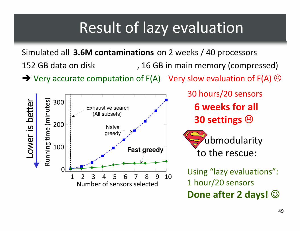
Simulated all on 2 weeks / 40 processors
152 GB data on disk
� Very accurate computation of F(A)
Using “lazy evaluations”:
1 hour/20 sensors
Done after 2 days! ☺☺☺☺
, 16 GB in main memory (compressed)
Lower is better
30 hours/20 sensors
6 weeks for all
30 settings ����
3.6M contaminations
Very slow evaluation of F(A) �
1 2 3 4 5 6 7 8 9 100
100
200
300
Number of sensors selected
Ru
nn
ing
tim
e (
min
ute
s)
Exhaustive search(All subsets)
Naivegreedy
Fast greedy
ubmodularity
to the rescue:
Result of lazy evaluation

50
What about worst-case?[Krause et al., NIPS ’07]
S2
S3
S4S1
Knowing the sensor locations, an
adversary contaminates here!
Where should we place sensors to quickly detect in the worst case?
Very different average-case impact,
Same worst-case impact
S2
S3
S4
S1
Placement detects
well on “average-case”
(accidental) contamination