active learning from imbalanced data: a solution of online

This article has been accepted for inclusion in a future issue of this journal. Content is final as presented, with the exception of pagination.

IEEE TRANSACTIONS ON NEURAL NETWORKS AND LEARNING SYSTEMS 1

Active Learning From Imbalanced Data: A Solutionof Online Weighted Extreme Learning Machine

Hualong Yu , Xibei Yang, Shang Zheng, and Changyin Sun

Abstract— It is well known that active learning can simultane-ously improve the quality of the classification model and decreasethe complexity of training instances. However, several previousstudies have indicated that the performance of active learningis easily disrupted by an imbalanced data distribution. Someexisting imbalanced active learning approaches also suffer fromeither low performance or high time consumption. To addressthese problems, this paper describes an efficient solution based onthe extreme learning machine (ELM) classification model, calledactive online-weighted ELM (AOW-ELM). The main contribu-tions of this paper include: 1) the reasons why active learningcan be disrupted by an imbalanced instance distribution andits influencing factors are discussed in detail; 2) the hierarchicalclustering technique is adopted to select initially labeled instancesin order to avoid the missed cluster effect and cold startphenomenon as much as possible; 3) the weighted ELM (WELM)is selected as the base classifier to guarantee the impartiality ofinstance selection in the procedure of active learning, and anefficient online updated mode of WELM is deduced in theory;and 4) an early stopping criterion that is similar to but moreflexible than the margin exhaustion criterion is presented. Theexperimental results on 32 binary-class data sets with differentimbalance ratios demonstrate that the proposed AOW-ELMalgorithm is more effective and efficient than several state-of-the-art active learning algorithms that are specifically designedfor the class imbalance scenario.

Index Terms— Active learning, class imbalance, cost-sensitivelearning, extreme learning machine (ELM), online learning,stopping criterion.

I. INTRODUCTION

ACTIVE learning is a popular machine learning paradigmand it is frequently deployed in the scenarios when large-

scale instances are easily collected, but labeling them is expen-sive and/or time-consuming [1]. By adopting active learning,

Manuscript received April 27, 2017; revised March 4, 2018 andJune 27, 2018; accepted July 3, 2018. This work was supported in part by theNational Natural Science Foundation of China under Grant 61305058 andGrant 61572242, in part by the Natural Science Foundation of JiangsuProvince of China under Grant BK20130471, in part by the China PostdoctoralScience Foundation under Grant 2013M540404 and Grant 2015T80481,in part by the Jiangsu Planned Projects for Postdoctoral Research Funds underGrant 1401037B, and in part by the Qing Lan Project of Jiangsu Province ofChina. (Corresponding author: Hualong Yu.)

H. Yu, X. Yang, and S. Zheng are with the School of Computer, JiangsuUniversity of Science and Technology, Zhenjiang 212003, China (e-mail:[email protected]; [email protected]; [email protected]).

C. Sun is with the School of Automation, Southeast University, Nanjing210096, China (e-mail: [email protected]).

Color versions of one or more of the figures in this paper are availableonline at http://ieeexplore.ieee.org.

Digital Object Identifier 10.1109/TNNLS.2018.2855446

a classification model can iteratively interact with humanexperts to only select those most significant instances forlabeling and to further promote its performance as quicklyas possible. Therefore, the merits of active learning lie indecreasing both the burden of human experts and the complex-ity of training instances but acquiring a classification modelthat delivers superior or comparable performance to the modelwith labeling all instances.

Past research has accumulated a large number of activelearning models, and generally, we have several different tax-onomies to organize these models. Based on different ways ofentering the unlabeled data, active learning can be divided intopool-based [2], [3] and stream-based models [4]. The formerpreviously collects and prepares all unlabeled instances, whilethe latter can only visit a batch of newly arrived unlabeled dataat each specific time point. According to different numbersof the labeled instances in each round, we have single-modeand batch-mode learning models [5]. As their names indicate,the single-mode model only labels one unlabeled instance oneach round, while the batch-mode labels a batch of unla-beled examples once. In addition, we have several differentsignificance measures to rank unlabeled instances, includinguncertainty [6], [7], representativeness [8], inconsistency [9],variance [10], and error [11]. Each significance measure has acriterion for evaluating which instances are the most importantfor improving the performance of the classification model. Forexample, uncertainty considers the most important unlabeledinstance to be the nearest one to the current classificationboundary; representativeness considers the unlabeled instancethat can represent a new group of instances, e.g., a cluster,to be more important, and inconsistency considers the unla-beled instance that has the most predictive divergence amongmultiple diverse baseline classifiers to be more significant.In addition, active learning models can also be divided intodifferent categories according to which kind of classifierhas been adopted. Some popular classifiers, including naiveBayes [12], k-nearest neighbors [13], decision tree [6], multi-ple level perceptron (MLP) [14], [15], logistic regression [16],support vector machine (SVM) [17]–[19], and extreme learn-ing machine (ELM) [20], [21], have all been developed tosatisfy the requirements of active learning. In the past decade,active learning has also been deployed in a variety of real-world applications, such as video annotation [22], [23], imageretrieval [18], [24], text classification [25], [26], remote sens-ing image annotation [27], speech recognition [28], networkintrusion detection [29], and bioinformatics [30].

2162-237X © 2018 IEEE. Personal use is permitted, but republication/redistribution requires IEEE permission.See http://www.ieee.org/publications_standards/publications/rights/index.html for more information.

https://orcid.org/0000-0001-9621-4158

https://orcid.org/0000-0001-9269-334X


2 IEEE TRANSACTIONS ON NEURAL NETWORKS AND LEARNING SYSTEMS

Active learning is undoubtedly effective, but several recentstudies have indicated that active learning tends to fail when itis applied to data with a skewed class distribution [25], [26],[31]–[33]. That is, similar to traditional supervised learning,active learning also dares to face class imbalance problem.Several previous studies have tried to address this prob-lem by using different techniques. Zhu and Hovy [25] firstnoticed this problem and tried to include several samplingtechniques in active learning procedure to control the balancebetween the number of labeled instances in the minorityand majority classes. Specifically, they presented three dif-ferent sampling techniques: random undersampling (RUS),random oversampling (ROS), and bootstrap-based oversam-pling (BootOS) [25]. The authors indicated that RUS is gener-ally worse than the original active learning algorithm, whereasboth ROS and BootOS can increase the performance oflearning, although the former tends to be more overfitting thanthe latter. Bloodgood and Vijay-Shanker [26] took advantageof the idea of cost-sensitive learning, which is another popularclass imbalance learning technique, to handle a skewed datadistribution during active learning. In particular, cost-sensitiveSVM (CS-SVM) was employed as the base learner, empiricalcosts were assigned according to the prior imbalance ratio, andtwo traditional stopping criteria, i.e., the minimum error andthe maximum confidence, were adopted to find the appropriatestopping condition for active learning. The method is robustand effective; however, it is also more time-consuming becausethe high time-complexity of training an SVM and no useof online learning. Tomanek and Hahn [31] proposed twomethods based on the inconsistency significance measure:balanced-batch active learning (AL-BAB) and active learningwith boosted disagreement (AL-BOOD), where the formerselects n labeled instances that are class balanced from 5nbnew labeled instances on each round of active learning, whilethe latter modifies the equation of voting entropy to makeinstance selection focus on the minority class. It is clear thatAL-BAB is quite similar to RUS, but it is possibly worseand wastes even more labeled resources than RUS, whileAL-BOOD must deploy many diverse base learners (ensem-ble learning) to calculate the voting entropy of predictivelabels, which will inevitably increase the computational bur-den. Therefore, we did not compare our proposed methodwith above-mentioned methods in Section V. In addition tothe methods mentioned earlier, there has been research onhow to treat the class imbalance problem by active learning.Ertekin et al. [32], [33] indicated that near the boundary oftwo different classes, the imbalance ratio is generally muchlower than the overall ratio, thus adopting active learning caneffectively alleviate the negative effects of imbalanced datadistribution. In other words, they consider active learning to bea specific sampling strategy. In addition, a margin exhaustioncriterion is proposed as an early stopping criterion to confirmthe stopping condition because they selected SVM as a baselearner.

To summarize the existing active learning algorithmsapplied in the scenario of unbalanced data distributions,we found that they suffer from either low classification per-formance or high time-consumption problems. Therefore, in

this paper, we wish to propose an effective and efficientalgorithm. The proposed algorithm is named active online-weighted ELM (AOW-ELM), and it should be applied inthe pool-based batch-mode active learning scenario with anuncertainty significance measure and ELM classifier. We selectELM as the baseline classifier in active learning based on threeobservations: 1) it always has better than or at least comparablegenerality ability and classification performance as do SVMand MLP [34], [35]; 2) it can tremendously save training timecompared to other classifiers [36]; and 3) it has an effectivestrategy for conducting active learning [21]. In AOW-ELM,we first take advantage of the idea of cost-sensitive learning toselect the weighted ELM (WELM) [37] as the base learner toaddress the class imbalance problem existing in the procedureof active learning. Then, we adopt the AL-ELM algorithm [21]presented in our previous paper to construct an active learningframework. Next, we deduce an efficient online learning modeof WELM in theory and design an effective weight updaterule. Finally, benefiting from the idea of the margin exhaustioncriterion, we present a more flexible and effective early stop-ping criterion. Moreover, we try to simply discuss why activelearning can be disturbed by skewed instance distribution,further investigating the influence of three main distributionfactors, including the class imbalance ratio, class overlapping,and small disjunction. Specifically, we suggest adopting theclustering techniques to previously select the initially labeledseed set, and thereby avoid the missed cluster effect andcold start phenomenon as much as possible. Experiments areconducted on 32 binary-class imbalanced data sets, and theresults demonstrate that the proposed algorithmic framework isgenerally more effective and efficient than several state-of-the-art active learning algorithms that were specifically designedfor the class imbalance scenario.

The rest of this paper is organized as follows. Section IIintroduces some priori knowledge related to this paper.In Section III, we construct several representative syntheticdata sets with different distributions to analyze the reason whyactive learning can be destroyed by skewed instance distribu-tion. Section IV presents our proposed algorithmic frameworkin detail. Section V provides the experimental results andanalysis. Finally, Section VI concludes the contributions ofthis paper and indicates future work.

II. PRELIMINARIES

In this section, we present some preliminaries, includingthe basic flow path of pool-based active learning, ELM,WELM, online sequential ELM, and active learning withELM (AL-ELM). The proposed core algorithmic model of thispaper is presented in Section IV.

A. Flow Path of Pool-Based Active Learning

As mentioned in Section I, according to different ways ofentering the unlabeled data, active learning can be divided intotwo categories: pool based [2], [3] and stream based [4], wherethe pool-based scenario is more common in real-world appli-cations. In pool-based scenario, all unlabeled instances arepreviously prepared, and then a fraction of them are randomly


YU et al.: ACTIVE LEARNING FROM IMBALANCED DATA: SOLUTION OF ONLINE WELM 3

Fig. 1. Flowchart of the pool-based active learning.

extracted and labeled by human experts, further executingactive learning iteratively. In other words, the classificationmodel can continuously select the useful instances from theunlabeled pool to promote quality. In this paper, we focus onthe pool-based active learning scenario.

The basic flow path of the pool-based active learningis described in Fig. 1. As we can see, the flow path isorganized into four parts, and it is a closed loop. In eachround, the labeled set is used to train a classification model.Then, the model estimates the significance of each instancein the unlabeled set, ranks them, and selects some of themost significant instances to submit to human annotators, whofurther provide labels for these instances and then insert theminto the training instances to update the labeled set. Activelearning repeats the process above until it satisfies a stoppingcondition. Obviously, in the flow path mentioned above, howto use the classification model to estimate, rank, and extractsignificant unlabeled instances is the key point because itdirectly concerns the quality of active learning.

B. Extreme Learning Machine

ELM that was proposed by Huang et al. [34], [35] isa specific learning algorithm for single-hidden layer feed-forward neural networks (SLFNs). The main characteristicsof ELM that distinguish it from those conventional learningalgorithms of SLFN are the random generation of hiddennodes. Therefore, ELM does not need to iteratively adjust theparameters to make them approach the optimal values, thusit has faster learning speed and better generalization ability.Previous research has indicated that ELM can produce betterthan or at least comparable generality ability and classifi-cation performance to SVM and MLP but only consumestenths or hundredths of training time compared to SVM andMLP [34]–[36].

Let us consider a classification problem with N traininginstances to distinguishing m categories, and then the i th train-ing instance can be represented as (xi , ti ), where xi is an n×1input vector and ti is the corresponding m× 1 output vector.Suppose there are L hidden nodes in ELM and that all weightsand biases on these nodes are generated randomly. Then, forthe instance xi , its hidden layer output can be represented as arow vector h(xi ) = [h1(xi ), h2(xi ), . . . , hL(xi )] by mappingwith an activation function (the most popular sigmoid function

is used throughout this paper). The mathematical model ofELM could be described as

Hβ = T (1)

where H = [h(x1), h(x2), . . . , h(xN )]T is the hidden layeroutput matrix overall training instances, β is the weight matrixof the output layer, and T = [t1, t2, . . . , tN ] denotes the targetmatrix. Obviously, in (1), only β is unknown, so we can adoptthe least-square algorithm to acquire its solution, which canbe described as follows:

β = H †T ={

H T (H H T )−1T, when N ≤ L

(H H T )−1 H T T, when N > L(2)

where H † denotes the Moore–Penrose generalized inverse ofthe hidden layer output matrix H , which can guarantee thesolution is the least-norm least-squares solution for (1).

We can also train an ELM in the viewpoint of optimization[35]. In the optimization version of ELM, we wish to synchro-nously minimize ‖Hβ − T ‖2 and ‖β‖2, so the question canbe described as follows:

min: LpELM = 1

2‖β‖2 + C

1

2

N∑i=1

‖ξi‖2

s.t: h(xi )β = tTi − ξT

i , i = 1, 2, . . . , N (3)

where ξi = [ξi,1, ξi,2, . . . , ξi,m ] denotes the training errorvector of the m output nodes with respect to the traininginstance xi , and C is the penalty factor representing thetradeoff between the minimization of training errors and themaximization of generality ability. Obviously, this is a typicalquadratic programming problem that can be solved by theKarush–Kuhn–Tucker theorem [38]. The solution for (3) canbe described as follows:

β = H †T =

⎧⎪⎪⎪⎨⎪⎪⎪⎩

H T(

I

C+ H H T

)−1

T, when N ≤ L(I

C+ H H T

)−1

H T T, when N > L .

(4)

C. Weighted Extreme Learning Machine

WELM that can be regarded as a cost-sensitive learningversion of ELM is an effective way to handle the imbalanceddata [37]. Similar to CS-SVM, the main idea of WELM isto assign different penalties for different categories, wherethe minority class has a larger penalty factor C , while themajority class has a smaller C value. Then, WELM focuseson the training errors of the minority instances, making aclassification hyperplane emerge in a more impartial position.A weighted matrix W is used to regulate the parameter C fordifferent instances, i.e., (3) can be rewritten as

min: LpELM = 1

2‖β‖2 + C

1

2W

N∑i=1

‖ξi‖2

s.t: h(xi )β = tTi − ξT

i , i = 1, 2, . . . , N (5)

where W is a N × N diagonal matrix in which each valueexisting on the diagonal represents the corresponding regula-tion weight of parameter C . Zong et al. [37] provided two



different weighting strategies that are described as follows:WELM1 : Wii = 1/#(ti ) (6)

and

WELM2 : Wii ={

0.618/#(ti) if #(ti ) > AVG(ti )

1/#(ti ) if #(ti ) ≤ AVG(ti )(7)

where #(ti ), average (AVG)(ti), and 0.618 denote the numberof instances belonging to the class ti , the average numberof instances over all classes, and the value of the goldenstandard, respectively. Compared with WELM2, WELM1 ismore practical and popular. Then, the solution can be describedas follows:

β =

⎧⎪⎪⎨⎪⎪⎩

H T(

I

C+ W H H T

)−1

W T, when N ≤ L(I

C+ H W H T

)−1

H T W T, when N > L .

(8)

D. Online Sequential Extreme Learning Machine

In 2006, Liang et al. [39] proposed an online sequentiallearning mode of ELM named oversampling (OS)-ELM. OS-ELM adopts extended recursive least squares for training withsequentially received data that can be either received in themode of one by one or chunk by chunk. Based on theirderivation, the update rule of the output layer weight matrixβ can be represented as

β(k+1) = β(k) + Pk+1 H Tk+1(Tk+1 − Hk+1β

(k)) (9)

where Hk+1 and Tk+1 correspond to the hidden layer outputmatrix and the target matrix of the new observations in the(k + 1)th chunks, while β(k) and β(k+1) denote the outputlayer weight matrix β after receiving the kth and (k + 1)thchunks, respectively. As for Pk+1, it can be calculated by thefollowing formula:

Pk+1 = Pk − Pk H Tk+1(I + Hk+1 Pk H T

k+1)−1 Hk+1 Pk (10)

that is, Pk can also be iteratively updated, and the initial P0can be represented as

P0 = (H T0 H0)

−1 (11)

where H0 indicates the premier hidden layer output matrix. Letus return to (9), as Hk+1, Tk+1, and Pk+1 all can be calculatedonly by the newly received instances. Thus, the output layerweight matrix β can be adjusted to adapt both old and newinstances, but it does not need to be recalculated with all ofthe training examples. It is not difficult to observe that themain merit of the OS-ELM algorithm is to decrease the time-complexity to a large extent when we can only acquire thetraining instances dynamically.

E. Active Learning With Extreme Learning Machine

In our previous work, we proposed an active learningalgorithm based on ELM and named it AL-ELM [21].We found that the actual outputs of ELM can reflect the uncer-tainty level of instances, i.e., their classification confidences.Specifically, we also proved that there is an approximate

TABLE I

DISTRIBUTIONS OF THE SIX SYNTHETIC DATA SETS

mapping relationship between the actual outputs of ELMand the posterior probabilities in the Bayes classifier. Themore approximate the actual outputs on different output nodesare, the more approximate the posterior probabilities belongingto the different classes are, and the more uncertain and impor-tant the corresponding instance is for modeling the classifier,too. As mentioned in Section I, labeling the most uncertaininstances, i.e., the instances that are the closest to the currentclassification hyperplane, may provide a maximum promotionfor the quality of the classification model. To convert thenonprobabilistic outputs in ELM into probabilistic outputs, weuse the sigmoid function as follows:

P(ti | fi (x)) = 1

1 + exp(− fi (x)), i = 1, 2, . . . ,m (12)

where ti = 1 means that category i happens, fi (x) denotesthe actual output of the i th output node with respect to theinstance x . For the binary-class problem, the accumulatedprobabilistic value on two output nodes strictly equals 1. Forthe multiclass problem, however, the sum of the convertedprobabilistic values is always larger than 1, thus we alsopresent a normalized strategy as follows:

P ′(ti | fi (x)) = P(ti | fi (x))∑mk=1 P(tk | fk(x))

, i = 1, 2, . . . ,m. (13)

In AL-ELM, we select the most uncertain instances, i.e., theinstances with the most approximate actual outputs in twodifferent output nodes, to a label on each round. In this paper,we inherit the uncertainty estimation and selection strategyin AL-ELM.

III. INVESTIGATION INTO THE DISTRIBUTION

To clarify why traditional active learning algorithms areeasily destroyed by a skewed data distribution, we exploreit from the perspective of data distribution. Here, we gen-erate six synthetic 2-D binary-class imbalanced data setswith considering three different data distribution factors: classimbalance ratio, class overlapping, and small disjunction. Thedistributions of these six data sets are summarized in Table I.

In Table I, we can observe that data sets D1–D4 satisfythe same distribution but have different class imbalance ratios,from 2:1 to 200:1. Although data set D5 has the same classimbalance ratio as D2 does, they satisfy different distributions,



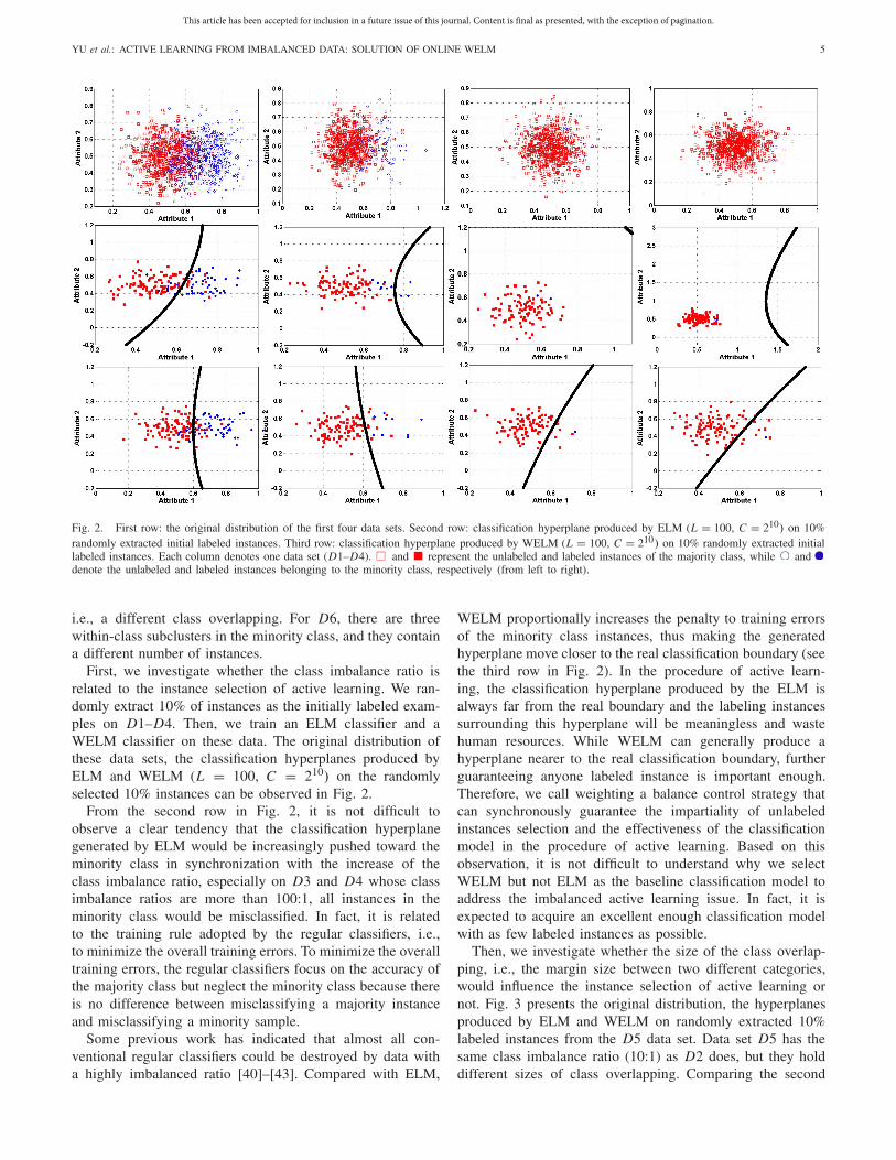
Fig. 2. First row: the original distribution of the first four data sets. Second row: classification hyperplane produced by ELM (L = 100, C = 210) on 10%randomly extracted initial labeled instances. Third row: classification hyperplane produced by WELM (L = 100, C = 210) on 10% randomly extracted initiallabeled instances. Each column denotes one data set (D1–D4). and represent the unlabeled and labeled instances of the majority class, while anddenote the unlabeled and labeled instances belonging to the minority class, respectively (from left to right).

i.e., a different class overlapping. For D6, there are threewithin-class subclusters in the minority class, and they containa different number of instances.

First, we investigate whether the class imbalance ratio isrelated to the instance selection of active learning. We ran-domly extract 10% of instances as the initially labeled exam-ples on D1–D4. Then, we train an ELM classifier and aWELM classifier on these data. The original distribution ofthese data sets, the classification hyperplanes produced byELM and WELM (L = 100, C = 210) on the randomlyselected 10% instances can be observed in Fig. 2.

From the second row in Fig. 2, it is not difficult toobserve a clear tendency that the classification hyperplanegenerated by ELM would be increasingly pushed toward theminority class in synchronization with the increase of theclass imbalance ratio, especially on D3 and D4 whose classimbalance ratios are more than 100:1, all instances in theminority class would be misclassified. In fact, it is relatedto the training rule adopted by the regular classifiers, i.e.,to minimize the overall training errors. To minimize the overalltraining errors, the regular classifiers focus on the accuracy ofthe majority class but neglect the minority class because thereis no difference between misclassifying a majority instanceand misclassifying a minority sample.

Some previous work has indicated that almost all con-ventional regular classifiers could be destroyed by data witha highly imbalanced ratio [40]–[43]. Compared with ELM,

WELM proportionally increases the penalty to training errorsof the minority class instances, thus making the generatedhyperplane move closer to the real classification boundary (seethe third row in Fig. 2). In the procedure of active learn-ing, the classification hyperplane produced by the ELM isalways far from the real boundary and the labeling instancessurrounding this hyperplane will be meaningless and wastehuman resources. While WELM can generally produce ahyperplane nearer to the real classification boundary, furtherguaranteeing anyone labeled instance is important enough.Therefore, we call weighting a balance control strategy thatcan synchronously guarantee the impartiality of unlabeledinstances selection and the effectiveness of the classificationmodel in the procedure of active learning. Based on thisobservation, it is not difficult to understand why we selectWELM but not ELM as the baseline classification model toaddress the imbalanced active learning issue. In fact, it isexpected to acquire an excellent enough classification modelwith as few labeled instances as possible.

Then, we investigate whether the size of the class overlap-ping, i.e., the margin size between two different categories,would influence the instance selection of active learning ornot. Fig. 3 presents the original distribution, the hyperplanesproduced by ELM and WELM on randomly extracted 10%labeled instances from the D5 data set. Data set D5 has thesame class imbalance ratio (10:1) as D2 does, but they holddifferent sizes of class overlapping. Comparing the second



Fig. 3. Original distribution, classification hyperplane produced by ELM (L = 100,C = 210) and WELM (L = 100,C = 210) on 10% randomly extractedinitial labeled instances of D5 data set, respectively. and represent the unlabeled and labeled instances of the majority class, while and denote theunlabeled and labeled instances belonging to the minority class, respectively.

Fig. 4. Distribution of the unlabeled set, the classification hyperplane produced by ELM (L = 100,C = 210) on 10% randomly extracted labeled instances,and the classification hyperplane produced by ELM (L = 100,C = 210) on 10% representative initially labeled instances on D6 data set, respectively.

and represent the unlabeled and labeled instances of the majority class, while and denote the unlabeled and labeled instances belonging to theminority class, respectively.

column in Fig. 2 with Fig. 3, we observe that on the largemargin class imbalance data set, the regular classifier, e.g.,ELM, generally produces a hyperplane that is nearer to themajority class than that produced on the small margin dataset. That is, the harmfulness will decrease in synchronizationwith the increase of margin size. However, it is still harmfulto regular classifiers, so adopting a balance control strategy isstill necessary (compare the second subgraph with the thirdsubgraph in Fig. 3).

Finally, we investigate the influence of a more complexdata distribution factor, i.e., within-class subclusters that arealso called small disjunction. There are several different sub-concepts or subdistributions in one class, and these subcon-cepts or subdistributions have a different number of instances.On the skewed data set with small disjunctions, we face boththe problem of “between-class imbalance” and the problem of“within-class imbalance” [44]. Taking the D6 data set as anexample, there are three within-class clusters with an imbal-ance ratio of 6:3:1 in the minority class. Then, a problem willappear, i.e., if none of the instances in the small subclustersare selected into the initially labeled set (seed set), then itis possible to permanently misclassify all instances belongingto these clusters. The problem is called the missed clustereffect [45]. To address this problem, we adopt the hierarchicalclustering technique to subtly explore the distribution structureof the collected unlabeled instances, further precisely selecting

and labeling those representative examples to construct theinitial seed set. Specifically, after hierarchical clustering isfinished, the instance that is closest to the centroid of eachcluster is extracted to label, as these instances are consideredthe representative instances. Fig. 4 presents the procedure ofseed sets generation by randomly extracting labeled instancesand selecting representative samples with the hierarchical clus-tering technique, and the classification hyperplanes producedby the ELM on these two seed sets. To simulate the actualprocedure of active learning, half of the instances in theD6 data set are randomly extracted to construct the initiallycollected unlabeled set, and then 10% of the examples in theunlabeled set is extracted randomly and selected carefully bythe clustering technique.

Fig. 4 indicates that if we randomly extract some instancesto construct the initially labeled seed set, some small subclus-ters may be missed and may even be permanently misclassifiedbecause they are far from the initial classification hyperplane.That means, these instances might not be labeled perma-nently during active learning. Hierarchical clustering, however,is helpful for finding those representative instances that canbetter describe the original data distribution. In addition, thistechnique is useful for avoiding the cold start phenomenon thatoften appears in the scenario of highly skewed data distribu-tion. Cold start means that none of the minority class instancesare selected into the seed set, resulting in the impracticability



of active learning [46]. Fig. 4 shows that the selection ofinitially labeled examples based on the clustering techniqueexplores all small distribution structures, and further extractsmore instances belonging to the minority class, thus it can beused to effectively reduce the probability of a cold start. In thispaper, all experiments are based on the seed set generatedby the hierarchical clustering technique, and the numberof subclusters equals the number of the initially labeledinstances.

The analysis mentioned above demonstrates that on imbal-anced distribution data, the performance of active learning canbe influenced by a combination of multiple factors and is notonly related to class imbalance ratio. Therefore, it is necessaryto conduct a balance control strategy during active learning,

IV. AOW-ELM ALGORITHM MODEL

A. Online Sequential Weighted Extreme Learning Machine

As we know, active learning conducts an iterative procedure,i.e., adding one or a batch of new labeled instances into thelabeled set each round. Undoubtedly, it would be quite time-consuming to retrain the classification model on each round.Therefore, it is necessary to adopt an online learning algorithmto implement active learning. Mirza et al. [47] presented anonline sequential WELM algorithm to address the incrementalclass imbalance learning problem. However, the algorithmis based only on the least-squares version and not on theoptimization version of ELM, thereby losing control of thegeneralization ability of ELM. In addition, the iterative weighttuning and ranking mechanism adopted in this algorithmincrease the unnecessary time expenditure. In [48], a kernel-based imbalance online learning algorithm was presented.The algorithm is effective in addressing imbalanced onlinelearning with concept drift. However, it has a limitation forapplication in our active learning scenario, i.e., its instanceweight is correlated with the number of training instancesbelonging to each class acquired to date, which means thatthe new instances’ weights will gradually decrease, while theold instances could be highlighted. Obviously, it cannot satisfyour application requirements. To avoid these problems, a novelonline sequential WELM algorithm based on the optimizationversion is proposed in this paper. Its derivation process issimilar to the OS-ELM algorithm [39].

Based on (8), we have

β =(

I

C+ H W H T

)−1

H T W T

=(

I

C+ (

√W H )T (

√W H )

)−1

(√

W H )T (√

W T ). (14)

Then, (14) can be rewritten as

β =(

I

C+ U T U

)−1

U T V (15)

where

U = √W H

V = √W T . (16)

Before the incremental learning starts, we only hold theinitially labeled seed set, thus the first classification modelcan be represented as follows:

β(0) =(

I

C+ U T

0 U0

)−1

U T0 V0 (17)

where

U0 =√

W0 H0

V0 = √W0T0 (18)

where W0, H0, and T0 are calculated with the initial seed set.Then, we consider the incremental procedure, for the (K +1)thiteration, the weight matrix of the output layer β could berepresented as

β(K+1) =(

I

C+ U T

K+�K UK+�K

)−1

U TK+�K VK+�K (19)

where

UK+�K = √WK+�K HK+�K =

[UK

U�K

]

VK+�K = √WK+�K TK+�K =

[VK

V�K

](20)

and �K indicates the (K + 1)th received the chunk of theincremental labeled instances. According to (20), (19) can bewritten as

β(K+1) =(

I

C+U T

K UK +U T�K U�K

)−1

(U TK VK +U T

�K V�K ).

(21)

Revisiting (17), let

P0 = I

C+ U T

0 U0. (22)

Combining (21) and (22), β(1) is given by

β(1) = (P0 + U T�1U�1)

−1U T0 V0 + U T

�1V�1 (23)

then P1 can be represented as

P1 = P0 + U T�1U�1 = I

C+ U T

1 U1. (24)

Thus, it is not difficult to deduce the expression of PK+1

PK 1 = PK + U T�K U�K = I

C+ U T

K UK + U T�K U�K . (25)

Combining (23) and (27), we have

β(K+1) = (PK + U T�K U�K )

−1(U TK VK + U T

�K V�K ). (26)

Then, we observe the second term in (28), it can betransferred to

U TK VK +U T

�K V�K = PK P−1K U T

K VK + U T�K V�K

= PK

(I

C+U T

K UK

)−1

U TK VK +U T

�K V�K

= PKβ(K ) + U T

�K V�K . (27)

Integrating the result into (28), we have

β(K+1) = (PK + U T�K U�K )

−1(PKβ(K ) + U T

�K V�K ). (28)



As PK can be incrementally updated, U�K and V�K aremerely correlated with the instances in the newly receivedchunk, thus β(K+1) can be deduced from β(K ).

By observing (28), it is clear that the time-complexity ofthe learning procedure mentioned above is linear with respectto the number of the incrementally labeled instances becausein each round, the new incremental training time is related toonly the number of newly labeled training instances. Becausethe quality of ELM is determined only by the weight matrixof the output layer β, updating β means the implementationof online incremental learning.

B. Weight Update Rule

Next, we focus on the problem of weight setting for thenewly received labeled instances during online learning. In thework of Zong et al. [37], the weight assignment is related tothe reciprocal of the number of the instances belonging toeach category. It is obviously improper to assign the weightsby this strategy, as with an increase in the number of labeledexamples, the weights used to punish the newly insertedinstances would decrease sharply, resulting in the classificationmodel focuses on the previous instances, but neglects thenewly labeled ones. In other words, we need a more robustweight assignment strategy that should be irrelevant to thetimeline. Here, we provide a stable weight update strategyfor online learning on binary-class skewed data. For a newlylabeled instance xi , its weight can be assigned as

wi =

⎧⎪⎪⎨⎪⎪⎩

|N+||N+| + |N−| , if xi belong to the majority class

|N−||N+| + |N−| , if xi belong to the minority class

(29)

where |N+| and |N−| denote the number of instances belong-ing to the positive class (minority class) and the negativeclass (majority class) in the currently labeled set, respectively.The weights rely only on the ratio between the number ofinstances belonging to two different classes, regardless of theabsolute number of instances, so it would be more stablethan (6) which might assign monotonically decreasing weightsto the new instances and further gradually reduce the effectof the newly learned instances. Furthermore, the ratio ofthe weights between two different classes reflects the classimbalance ratio. However, during online learning, the ratio stillfluctuates dynamically.

C. Early Stopping Criterion

As we know, the objective of active learning is to acquirea high-quality classification model in synchronization withreducing the number of labeled instances. Therefore, exhaust-ing all unlabeled instances is unacceptable in practical activelearning applications. In fact, an early stopping criterionshould be previously designated to ask active learning when itshould be stopped. The optimal stopping time should simulta-neously guarantee two conditions: 1) the performance of the

Fig. 5. Classification hyperplane (black line), contour lines (gray lines)directed by four different thresholds (0.1, 0.3, 0.5, and 1.0), and their marginranges produced by WELM (L = 100,C = 210) on 10% randomly extractedlabeled instances on D5 data set. and represent the unlabeled and labeledinstances of the majority class, while and denote the unlabeled andlabeled instances belonging to the minority class, respectively.

current classification model should be good enough and 2) thesize of the total labeled instances should be small enough.

In this paper, we refer to the idea of the margin exhaustioncriterion presented in the work of Ertekin et al. [33], and thendesign a more flexible early stopping criterion. Unlike SVM,there is no concept about margin in ELM, but in our previouswork, we observed that the contour line of a designated actualoutput value in ELM could be used to describe the confidencedistribution, while a pair of contour lines can direct a so-calledmargin. Fig. 5 presents the margin ranges beyond four differentthresholds constructing on 10% randomly labeled instancesof the D5 data set trained by WELM. Threshold μ denotesthe actual output absolute value of the output node. Thus,a specific threshold μ corresponds to a pair of contour linesthat indicate a margin. With an increase in the threshold μ,the margin will become larger. It is clear that the larger thethreshold μ is designated, the lower the acceptable uncertaintylevel is, thus more instances must be labeled in the activelearning procedure.

In this paper, margin exhaustion means that for a giventhreshold μ, finding two corresponding contour lines in theinstance space, when and only when all instances layingbetween these two contour lines have been labeled, activelearning can be stopped. Of course, in practical applications,we do not need to describe the contour lines, but only comparethe actual output of an instance with the given threshold todetermine whether the instance drops into the margin. In addi-tion, the actual output of ELM can be considered a variantof posterior probability, so the proposed stopping criterionis also approximately equivalent to the maximum confidencestopping criterion [49]. Therefore, it is not difficult to observethat the proposed early stopping criterion is both effective andmore flexible than the traditional margin exhaustion criterion.A discussion of the threshold μ is given in Section V.

D. AOW-ELM Algorithm Description

In this section, we expect to describe the detailed procedureof the AOW-ELM algorithm as follows.



TABLE II

DATA SETS USED IN THIS PAPER

1) Algorithm: AOW-ELM.2) Input: A collected unlabeled instance set �, the number

of initially labeled instances κ , the initially labeled setψ = φ, the number of labeled instances on each roundυ, the number of the hidden nodes L, the penalty factorC , and the stopping threshold μ.

3) Output: The final weight matrix β(F).4) Procedure.

a) Clustering all instances in� into κ different groupsby hierarchical clustering technique.

b) Find the instance that is closest to the centroid ineach cluster extract and label them, and then shiftthem from � to ψ .

c) Count and record the number of minority instances|N+| and majority instances |N−| in ψ .

d) Adopt (29) to calculate and acquire the initialweighting matrix W0.

e) Generate the hidden-layer parameters randomly forL hidden nodes.

f) Calculate β(0) using (8) and P0 using (22).g) Calculate the actual output of each instance in �,

if there exist outputs smaller than the threshold μ,continue to conduct the next step, else, stop, andreturn the current β as β(F).

h) Rank all instances in � according to their actualoutput absolute values in ascending order, and thenextract υ first instances to submit to human expertsfor labeling.

i) Transfer υ new labeled instances from � to ψ .j) Update |N+| and |N−|, and assign the weights for

these υ new labeled instances using (29).k) Compute U�K and V�K for υ new labeled

instances taking advantage of the random parame-ters generated for the hidden layer in step. e.

l) Update P using (25).m) Update β using (28), and then return to step. g.

V. EXPERIMENTS

A. Data Sets

In this paper, we focus on conducting active learning onbinary-class imbalanced data. Overall, 32 binary-class imbal-anced data sets that are used, most of which come from theUniversity of California-Irvine (UCI) machine learning datarepository [50], and the others are from several publicationsabout bioinformatics [51]–[53]. These data sets have differentnumber of instances, number of features, and class imbalanceratios. In addition, for each data set, half of the instancesare reserved as the test set, and in the other half, a specificpercentage of instances is extracted as an initially labeled seedset. The percentage correlates with the size of the data set andclass imbalance ratio to avoid cold starts as much as possible.Furthermore, the batch size of active learning, i.e., the numberof instances labeled on each round, is also associated with thesize of data set. The detailed description and settings aboutthese data sets are provided in Table II.

B. Parameter Settings

To show the effectiveness of the proposed AOW-ELMalgorithm, we compare it with six other algorithms.

1) AO-ELM: It combines the AL-ELM algorithm [35] withthe OS-ELM algorithm [39], but does not adopt thebalance control strategy during active learning. In fact,it can be regarded as a baseline algorithm that is usedto indicate the necessity of a balance control strategy.

2) Random Online-sequential Weighting (ROW)-ELM: Itadopts online sequential WELM, but on each round,the new incremental samples are selected randomly.It can also be seen as a baseline algorithm to make clearthe necessity of active learning.

3) RUS-ELM [25]: It adopts RUS as the balance controlstrategy in the procedure of active learning. Specifically,it is required to reserve the current undersampling set to



TABLE III

PERFORMANCE (ALC METRIC) COMPARISON OF VARIOUS ALGORITHMS

conduct undersampling on next round, thus we did notadopt online learning in this algorithm.

4) ROS-ELM [25]: It adopts ROS as the balance controlstrategy in the procedure of active learning. In par-ticular, during active learning, all currently labeledinstances must be reserved for generating the over-sampling instances on the next round. In each round,a new increased oversampling set will be learnedincrementally.

5) BootOS-ELM [25]: It adopts the BootOS algorithmas the balance control strategy in the procedure ofactive learning. The procedure of BootOS is similar toROS. Parameter K in BootOS was designated a defaultvalue 5. When the number of the labeled instancesbelonging to the minority class is smaller than K ,it adopts ROS to copy minority instances.

6) Active Cost Sensitive (ACS)-SVM [26]: CS-SVM isadopted as the balance control strategy during activelearning, and SVM is used as the baseline classifier. Allparameters inherit from [26].

All algorithms were implemented in MATLAB 2013a envi-ronment, and experiments were conducted on an Intel(R) Corei7 6700HQ 8 cores CPU (main frequency: 2.60 GHz for eachcore) and 16-GB RAM.

To evaluate the performance of each algorithm at a specifictime point to construct the learning curve, we adopted theG-mean metric that can be calculated as

G-mean = √Acc+ × Acc− (30)

where Acc+ and Acc− denote the accuracy of the minorityclass and the majority class, respectively. The G-mean metricevaluates the tradeoff between the accuracy of the minority

class and that of the majority class. Then, to evaluate thequality of the overall learning procedure, we adopt a popularactive learning evaluation metric: area under the learningcurve (ALC) [54]. The ALC metric is calculated based onthe G-mean values of all time points on the learning curve.Therefore, we can say that the G-mean metric here is only usedto serve for the ALC metric. To compare various algorithmsfairly, the ALC metric was calculated upon exhausting allunlabeled instances.

For each algorithm related to ELM, a sigmoid functionis used to calculate the hidden-layer output matrix, and twomain parameters L and C are determined by grid search,where L ∈ {10, 20, . . . , 200} and C ∈ {2−4, 2−2, . . . , 220}.For ACS-SVM, the Gaussian radial basis kernel function isadopted, and the penalty factor C and the width parameter σare also tuned by grid search, where C ∈ [2−8, 2−7, . . . , 28]and σ ∈ [2−8, 2−7, . . . , 28].

Considering the randomness of the experiments, the experi-mental results may be unstable. Therefore, we adopt 50 timesrandom fivefold cross-validation to calculate the average resultfor each algorithm.

C. Comparison of Classification Performance

We first test the ALC metric of various compared algorithmson 32 given data sets. Table III presents the average resultsof 50 times random fivefold cross-validation.

We can see from Table III that on most data sets, thealgorithms with the balance control strategy improve theperformance to some extent. That means that inserting bal-ance control strategy into the procedure of active learningis effective and necessary. However, on several other datasets, including vowel0, banknote-authentication, segmentation



grass and magic, the promotion is not clear. Specifically,on the data sets mentioned earlier, it is possible to reducethe performance for those algorithms with the balance controlstrategy. As discussed in Section III, the performance of activelearning upon the skewed data distribution has a relationshipwith multiple factors. Therefore, we consider that there mightbe a low imbalance ratio, large class margin, and no existenceof small disjunctions in those four data sets. In fact, we observethat the imbalance ratio of those data sets is indeed very low.As expected, the results testify our hypothesis.

For sampling-based active learning algorithms, BootOS-ELM significantly outperforms ROS-ELM on a majority ofthe data sets, as it effectively alleviates the overfitting ofthe classification model, further help to extract more usefulunlabeled instances during active learning. It is also surprisingthat RUS-ELM can produce a quite high performance on manydata sets, which is not in accordance with the conclusion ofZhu and Hovy [25]. Zhu and Hovy [25] thought that the RUSstrategy had two obvious drawbacks as follows: 1) RUS wastedmany labeled instances and 2) RUS had a distinct reduction inperformance. In fact, when we seriously examined the resultsin Table III, it was not difficult to observe that RUS-ELM gen-erally performed better on those highly imbalanced data sets,such as abalone19, page-blocks5, microRNA, and Box H/ACAsnoRNA. Of course, the performance of the RUS-ELM algo-rithm was quite unstable, it produced significantly lower ALCmetrics on some data sets, e.g., 0.0000 on the magic dataset. Therefore, we suggest using it with caution in practicalapplications.

When comparing ROW-ELM with the proposed AOW-ELMalgorithm, we see that on a majority of the data sets,AOW-ELM significantly outperforms ROW-ELM, indicatingthat uncertainty-based instance selection can be faster thanrandom instance selection to improve the quality of the classi-fication model. In other words, the results also demonstrate theeffectiveness of our proposed uncertainty estimation and selec-tion strategy in the work of Yu et al. [21]. In addition, we alsonote that on several highly imbalanced data sets, ROW-ELMoften performed better than AOW-ELM. We think that onthese data sets, there may have existed much more noise thatcould influence the accuracy of uncertainty estimation, therebyuncertainty sampling was even worse than random sampling.

In contrast to the ACS-SVM algorithm [26], our proposedAOW-ELM algorithm seems not to be obviously superior.In particular, ACS-SVM achieves the best results on 12 datasets, while the best results of AOW-ELM only cover 11 datasets. Considering that they both adopt the idea of cost-sensitive learning as a balance control strategy, it is notdifficult to understand why they had similar performance.Here, the distinction between ACS-SVM and AOW-ELM ismerely correlated with different classification models adoptedby them. On these data sets, SVM outperforms ELM, whileon the other data sets, ELM outperforms SVM.

To present a thorough understanding of the comparison ofvarious algorithms, we also provide their statistical results.Specifically, the Friedman test is used to detect a significantdifference among a group of results, and the Holm post hoctest is adopted to examine whether the proposed algorithm is

TABLE IV

STATISTICAL RESULTS OF VARIOUS ALGORITHMS

distinctive among a 1 × N comparison [55], [56]. The posthoc procedure allows us to know whether a hypothesis ofcomparison of means could be rejected at a specified level ofsignificance α. The adjusted p-value (APV) is also calculatedto denote the lowest level of significance of a hypothesis thatresults in a rejection. Furthermore, we consider the averagerankings of the algorithms to measure how good an algorithmis with respect to its partners. The ranking could be calculatedby assigning a position to each algorithm depending on itsperformance on each data set. The algorithm that achieves thebest performance on a specific data set will be given rank 1(value 1), then the algorithm with the second-best result isassigned rank 2, and so forth. This task is conducted over alldata sets, and finally an average ranking is calculated. Thestatistical results are presented in Table IV.

Table IV shows that our proposed AOW-ELM algorithmachieved the lowest average ranking, indicating that it isthe best among all the algorithms. In addition, we observethat the APVs of the AO-ELM, RUS-ELM, ROS-ELM, andBootOS-ELM are lower than a standard level of significanceof α = 0.05. That means that these four algorithms are sig-nificantly different from the proposed AOW-ELM algorithm.However, we cannot say that AOW-ELM is significantlydifferent from ROW-ELM and ACS-SVM, although it has alower APV value than those two algorithms.

Fig. 6 presents the learning curves of seven comparedalgorithms on three representative data sets. In Fig. 6, the firstsubgraph is representative of most data sets that have amedium imbalance ratio and class overlapping. On this typeof data set, all algorithms could rapidly promote the qualityof the classification model in the initial stage of active learn-ing, and then the learning curves would be steady or evendeclining. As expected, AOW-ELM has a faster learning speedthan ROW-ELM, which demonstrates the effectiveness of theuncertainty-based instance selection strategy again. The sec-ond subgraph presents the learning curves generated on highlyimbalanced data sets. As we know, on the data sets with ahigh imbalance ratio, there generally exists noise, and mostminority instances are even embedded into the majority class;therefore, RUS may be more helpful for eliminating noiseand promoting the quality of the classification model. ForAO-ELM, which does not adopt any balance control strategy,all minority instances can be even misclassified. Of course,on this type of data set, our proposed algorithm is alsoeffective to some extent, but generally, it is not the best choice.



Fig. 6. Learning curves of seven compared active learning algorithms on three representative data sets: yeast-ME3, abalone19, and segmentation-grass,respectively (from left to right).

Fig. 7. Comparison of seven compared algorithms on the number of labeled instances belonging to the minority class in synchronization with the increaseof labeling rounds on three representative data sets: cardiotocographyc1, seed2, and abalone19, respectively (from left to right).

The third subgraph in Fig. 6 generally represents the easydata sets that have a low imbalance ratio, large class margin,and low noise. Therefore, we can observe that there is noclear distinction among different learning algorithms exceptRUS-ELM. Obviously, for this type of data sets, RUS is notan excellent balance control strategy, and even the learningalgorithm without a balance control strategy can generate goodperformance.

In addition to the observations discussed earlier, we also seean interesting phenomenon that although AOW-ELM generallyperforms better than ROW-ELM in the initial stage of activelearning, it could be surpassed gradually. We think that thisresult is related to the proposed weight update rule. Actually,uncertainty-based sampling strategy often tends to collectmore minority instances than a random sampling strategyin the initial stage of active learning. For the AOW-ELMalgorithm, the total weights assigned to the minority instancesis likely higher than that assigned for the majority instances,causing the later classification models to focus on the minor-ity class, and then reduce the G-mean metric. Fortunately,in practical applications, we generally do not need to exhaustall unlabeled instances, so AOW-ELM is still a better choicethan ROW-ELM.

Tomanek and Hahn [31] thought that an excellent activelearning algorithm constructing upon the skewed data distrib-ution should collect the unlabeled minority instances rapidlyin the initial stage of learning. Here, we examined the risingtrend of the minority labeled instances during active learning

for each compared algorithm on three representative data sets,named cardiotocographyC1, seed2, and abalone19 (see Fig. 7).

The first subgraph in Fig. 7 presents a common trend thatexisted on most of the data sets. Here, the curve of ROW-ELMcould be regarded as a benchmark, as it is approximatelylinear with respect to the imbalance ratio of the initiallyunlabeled set. As we can see in the first subgraph, all six otheralgorithms discover many more minority unlabeled instancesthan ROW-ELM does in the early stage of active learning.In particular, the AO-ELM algorithm could even exhaust allunlabeled minority instances approximately halfway throughthe learning. It is not difficult to understand the phenomenonby reviewing the discussions in Section III. Due to AO-ELMnot adopting any balance control strategy, the classificationhyperplane tends to appear in the region of the minorityclass, causing more minority instances to be extracted inthe early stage of active learning. In contrast with severalother algorithms, our proposed algorithm presents a moremoderate trend, indicating that discovering more unlabeledminority instances in the early stage of learning should behelpful for promoting the quality of the classification modelrapidly, but excessive extraction may be unwanted. The secondsubgraph in Fig. 7 is based on an easy data set. That means,in this type of data set, there existed a large margin betweenthe instances belonging to the two different classes. As weknow, for those easy data sets, nearly all learning algorithmscould acquire satisfying results, thus they all approximatelypresent a linear relation with the imbalance ratio of the



TABLE V

RUNNING TIME (SECONDS) COMPARISON OF VARIOUS ALGORITHMS

initially unlabeled set. For those difficult data sets that have ahigh imbalance ratio, large class overlapping, and high noise,all algorithms with uncertainty sampling can help discovermore unlabeled minority instances than the benchmark, i.e.,ROW-ELM, in the early stage of learning.

In our experiments, we have not run the proposed algorithmon multiclass data sets. In fact, on multiclass imbalancescenarios, two main challenges are presented: 1) cold startfrequently happens as the instances belonging to some classesare extremely scarce and 2) the weight updating rule willlose efficacy as most multiclass imbalanced data sets arehighly skewed. We believe that the cold start problem hasto be solved by some participation by human experts, and thesecond problem could be addressed by improving the weightupdating rule to equifrequently extract unlabeled instancesfrom different classes during active learning

D. Comparison of Running Time

Nevertheless, we should also consider the computation time.From Table V, we can see that AOW-ELM generally has asimilar running time as AO-ELM and ROW-ELM do, butneeds less running time than several other algorithms do.This is because both RUS-ELM and ACS-SVM do not adoptincremental learning, ROS-ELM wastes some time to copy theminority instances, while BootOS-ELM consumes much timeon neighborhood computation and synthetic instance genera-tion. Therefore, we can say that AOW-ELM is a time-savingalgorithm. Its superiority would be increasingly obvious insynchronization with increases in the instances and attributesexisting in a data set. Of course, the comparison betweenACS-SVM and AOW-ELM may be unfair as ACS-SVM doesnot adopt incremental learning. However, considering thattraining an individual SVM classification model is generally

much more time-consuming than training an ELM model,we believe AOW-ELM would still be more time-saving thanACS-SVM with incremental learning.

E. Discussion About Stopping Condition

Finally, we wish to discuss the stopping condition to makeclear the optimal setting for the threshold μ. We randomlyselect three representative data sets that reflect the concepts ofeasy, medium, and difficult. We let μ increase from 0.1 to 1.0with an increment of 0.1, and then the distinction betweenthe performance of each stopping point and the overall bestperformance was presented in Fig. 8.

In Fig. 8, we observe an approximately uniform trend onthe three different data sets. That is, at the beginning, thedistinction always decreased sharply in synchronization withthe increase of the threshold μ, and it then gradually becamestable. It is easy to understand this phenomenon: the thresholddenotes the maximum confidence level. As the thresholdincreases, more uncertain instances have been labeled, so theclassification model must be closer to the optimal performance.Although the trends are similar on the three different data sets,their best thresholds corresponding to the inflection points aretotally different. On the easy data set seed2, μ = 0.3 couldguarantee to acquire a good enough performance, while onthe medium data set cardiotocographyC1, the best thresholdis 0.4. For the difficult data set Box H/ACA snoRNA, when thethreshold μ equals 0.6, it provides the best tradeoff betweenthe classification performance and labeling expenses. Revisit-ing Fig. 5, it is not difficult to understand the phenomenonearlier. In Fig. 5, a small threshold means exhausting theinstances in a narrow margin surrounding the classificationboundary, while a large threshold means enlarging the marginand exhausting more instances. Considering the easy data



Fig. 8. Difference between the performance of each stopping point (denoting by a specific threshold μ) and the best performance on three representativedata sets: seed2, cardiotocographyC1, and Box H/ACA snoRNA, respectively (from left to right).

sets, which have low imbalance ratio and small classificationoverlapping, a small threshold is enough to guarantee preciselydescribing the classification boundary. However, for thosedifficult data sets with a high imbalance ratio, large class over-lapping, high noise, and even small disjunctions, we have toassign a large threshold for them to construct excellent enoughclassification models. In practical applications, the readers aresuggested to examine the instance distribution on the initiallylabeled set, and then allocate an appropriate threshold.

VI. CONCLUSION

In this paper, we explore the problem of active learn-ing in class imbalance scenario, and present a solution ofonline WELM named the AOW-ELM algorithm. We findthat the harmfulness of skewed data distribution is relatedto multiple factors, and can be seen as a combination ofthese factors. Hierarchical clustering can be effectively usedto previously extract initial representative instances into aseed set to address the potential missed cluster effect andcold start phenomenon. The comparison between the proposedAOW-ELM algorithm and some other benchmark algorithmsindicates that AOW-ELM is an effective strategy to addressthe problem of active learning in a class imbalance scenario.The merits of the AOW-ELM algorithm can be summarizedas follows.

1) It has a robust weight update rule.2) Its running time is fast and linear with the training

instances.3) It has a flexible early stopping criterion.4) It is appropriate for various types of data sets.In the future work, we will focus more on the problem of

active learning on multiclass imbalanced data sets. In addi-tion, the active learning strategies addressing imbalanced andunlabeled data streams with handling concept drifts will alsobe investigated.

REFERENCES

[1] B. Settles, “Active learning literature survey,” Dept. Comput. Sci., Univ.Wisconsin-Madison, Madison, WI, USA, Tech. Rep. 1648, Jan. 2010.

[2] M. Sugiyama and S. Nakajima, “Pool-based active learning in approx-imate linear regression,” Mach. Learn., vol. 75, no. 3, pp. 249–274,2009.

[3] A. K. McCallumzy and K. Nigam, “Employing EM and pool-based active learning for text classification,” in Proc. ICML, 1998,pp. 359–367.

[4] J. Smailovic, M. Grcar, N. Lavrac, and M. Žnidaršic, “Stream-basedactive learning for sentiment analysis in the financial domain,” Inf. Sci.,vol. 285, pp. 181–203, Nov. 2014.

[5] S. C. H. Hoi, R. Jin, J. Zhu, and M. R. Lyu, “Batch mode active learningand its application to medical image classification,” in Proc. ICML, 2006,pp. 417–424.

[6] D. Lewis and J. Catlett, “Heterogeneous uncertainty sampling forsupervised learning,” in Proc. ICML, 1994, pp. 148–156.

[7] M. Lindenbaum, S. Markovitch, and D. Rusakov, “Selective sampling fornearest neighbor classifiers,” Mach. Learn., vol. 54, no. 2, pp. 125–152,2004.

[8] S. Dasgupta and D. Hsu, “Hierarchical sampling for active learning,” inProc. ICML, 2008, pp. 208–215.

[9] R. Wang, S. Kwong, and D. Chen, “Inconsistency-based active learn-ing for support vector machines,” Pattern Recognit., vol. 45, no. 10,pp. 3751–3767, 2012.

[10] S. C. H. Hoi, R. Jin, and M. R. Lyu, “Large-scale text categorizationby batch mode active learning,” in Proc. WWW, 2006, pp. 633–642.

[11] N. Roy and A. McCallum, “Toward optimal active learning throughMonte Carlo estimation of error reduction,” in Proc. ICML, 2001,pp. 441–448.

[12] D. D. Lewis and W. A. Gale, “A sequential algorithm for training textclassifiers,” in Proc. ACM SIGIR, 1994, pp. 3–12.

[13] J. He and J. G. Carbonell, “Nearest-neighbor-based active learning forrare category detection,” in Proc. NIPS, 2008, p. 633–640.

[14] A. Krogh and J. Vedelsby, “Neural network ensembles, cross validation,and active learning,” in Proc. NIPS, 1995, pp. 231–238.

[15] K. Fukumizu, “Statistical active learning in multilayer perceptrons,”IEEE Trans. Neural Netw., vol. 11, no. 1, pp. 17–26, Jan. 2000.

[16] A. I. Schein and L. H. Ungar, “Active learning for logistic regression:An evaluation,” Mach. Learn., vol. 68, no. 3, pp. 235–265, 2007.

[17] S. Tong and D. Koller, “Support vector machine active learningwith applications to text classification,” J. Mach. Learn. Res., vol. 2,pp. 45–66, Nov. 2001.

[18] S. Tong and E. Chang, “Support vector machine active learning forimage retrieval,” in Proc. 9th ACM Int. Conf. Multimedia, 2001,pp. 107–118.

[19] Y. Qi and G. Zhang, “Strategy of active learning support vector machinefor image retrieval,” IET Comput. Vis., vol. 10, no. 1, pp. 87–94, 2016.

[20] C. Pan, D. S. Park, H. Lu, and X. Wu, “Color image segmentation byfixation-based active learning with ELM,” Soft Comput., vol. 16, no. 9,pp. 1569–1584, 2012.

[21] H. Yu, C. Sun, W. Yang, X. Yang, and X. Zuo, “AL-ELM:One uncertainty-based active learning algorithm using extreme learningmachine,” Neurocomputing, vol. 166, pp. 140–150, Oct. 2015.

[22] H. Liao, L. Chen, Y. Song, and H. Ming, “Visualization-based activelearning for video annotation,” IEEE Trans. Multimedia, vol. 18, no. 11,pp. 2196–2205, Nov. 2016.

[23] M. Wang and X. S. Hua, “Active learning in multimedia annotation andretrieval: A survey,” ACM Trans. Intell. Syst. Technol., vol. 2, no. 2,p. 10, 2011.

[24] P. H. Gosselin and M. Cord, “Active learning methods for interac-tive image retrieval,” IEEE Trans. Image Process., vol. 17, no. 7,pp. 1200–1211, Jul. 2008.

[25] J. Zhu and E. H. Hovy, “Active learning for word sense disambiguationwith methods for addressing the class imbalance problem,” in Proc.EMNLP-CoNLL, 2007, pp. 783–790.



[26] M. Bloodgood and K. Vijay-Shanker, “Taking into account the differ-ences between actively and passively acquired data: The case of activelearning with support vector machines for imbalanced datasets,” in Proc.Hum. Lang. Technol., 2009, pp. 137–140.

[27] S. Rajan, J. Ghosh, and M. M. Crawford, “An active learning approachto hyperspectral data classification,” IEEE Trans. Geosci. Remote Sens.,vol. 46, no. 4, pp. 1231–1242, Apr. 2008.

[28] G. Riccardi and D. Hakkani-Tur, “Active learning: Theory and appli-cations to automatic speech recognition,” IEEE Trans. Speech AudioProcess., vol. 13, no. 4, pp. 504–511, Jul. 2005.

[29] Y. Li and L. Guo, “An active learning based TCM-KNN algorithm forsupervised network intrusion detection,” Comput. Secur., vol. 26, no. 7,pp. 459–467, 2007.

[30] W. Xiong, L. Xie, S. Zhou, and J. Guan, “Active learning for proteinfunction prediction in protein–protein interaction networks,” Neurocom-puting, vol. 145, pp. 44–52, Dec. 2014.

[31] K. Tomanek and U. Hahn, “Reducing class imbalance during activelearning for named entity annotation,” in Proc. 5th Int. Conf. Knowl.Capture, 2009, pp. 105–112.

[32] S. Ertekin, J. Huang, and C. L. Giles, “Active learning for classimbalance problem,” in Proc. SIGIR, 2007, pp. 823–824.

[33] S. Ertekin, J. Huang, L. Bottou, and C. L. Giles, “Learning on the border:Active learning in imbalanced data classification,” in Proc. CIKM, 2007,pp. 127–136.

[34] G.-B. Huang, Q.-Y. Zhu, and C.-K. Siew, “Extreme learningmachine: Theory and applications,” Neurocomputing, vol. 70, nos. 1–3,pp. 489–501, 2006.

[35] G.-B. Huang, H. Zhou, X. Ding, and R. Zhang, “Extreme learningmachine for regression and multiclass classification,” IEEE Trans. Syst.,Man, Cybern. B, Cybern., vol. 42, no. 2, pp. 513–529, Apr. 2012.

[36] G. Huang, G.-B. Huang, S. Song, and K. You, “Trends in extreme learn-ing machines: A review,” Neural Netw., vol. 61, pp. 32–48, Jan. 2015.

[37] W. Zong, G.-B. Huang, and L. Chen, “Weighted extreme learn-ing machine for imbalance learning,” Neurocomputing, vol. 101,pp. 229–242, Feb. 2013.

[38] R. Fletcher, “Constrained optimization,” in Practical Methods of Opti-mization, vol. 2. Hoboken, NJ, USA: Wiley, 1981.

[39] N.-Y. Liang, G.-B. Huang, P. Saratchandran, and N. Sundararajan,“A fast and accurate online sequential learning algorithm for feedforwardnetworks,” IEEE Trans. Neural Netw., vol. 17, no. 6, pp. 1411–1423,Nov. 2006.

[40] N. Japkowicz and S. Stephen, “The class imbalance problem:A systematic study,” Intell. Data Anal., vol. 6, no. 5, pp. 429–450,2002.

[41] V. López, A. Fernández, S. García, V. Palade, and F. Herrera, “An insightinto classification with imbalanced data: Empirical results and cur-rent trends on using data intrinsic characteristics,” Inf. Sci., vol. 250,pp. 113–141, Nov. 2013.

[42] H. Yu, C. Mu, C. Sun, W. Yang, X. Yang, and X. Zuo, “Supportvector machine-based optimized decision threshold adjustment strategyfor classifying imbalanced data,” Knowl.-Based Syst., vol. 76, pp. 67–78,Mar. 2015.

[43] H. Yu, C. Sun, X. Yang, W. Yang, J. Shen, and Y. Qi, “ODOC-ELM:Optimal decision outputs compensation-based extreme learning machinefor classifying imbalanced data,” Knowl.-Based Syst., vol. 92, pp. 55–70,Jan. 2016.

[44] H. He and E. A. Garcia, “Learning from imbalanced data,” IEEE Trans.Knowl. Data Eng., vol. 21, no. 9, pp. 1263–1284, Sep. 2009.

[45] K. Tomanek, F. Laws, U. Hahn, and H. Schütze, “On proper unit selec-tion in active learning: co-selection effects for named entity recognition,”in Proc. NAACL HLT Workshop Act. Learn. Natural Lang. Process.,2009, pp. 9–17.

[46] H. He and Y. Ma, Imbalanced Learning: Foundations, Algorithms, andApplications. Hoboken, NJ, USA: Wiley, 2013.

[47] B. Mirza, Z. Lin, and K.-A. Toh, “Weighted online sequential extremelearning machine for class imbalance learning,” Neural Process. Lett.,vol. 38, no. 3, pp. 465–486, 2013.

[48] S. Ding et al., “Kernel based online learning for imbalance multiclassclassification,” Neurocomputing, vol. 277, pp. 139–148, Feb. 2018.

[49] J. Zhu, H. Wang, E. Hovy, and M. Ma, “Confidence-based stoppingcriteria for active learning for data annotation,” ACM Trans. SpeechLang. Process., vol. 6, no. 3, p. 3, 2010.

[50] C. Blake, E. Keogh, and C. J. Merz, UCI Repository of MachineLearning Databases, Dept. Inf. Comput. Sci., Univ. California, Irvine,CA, USA, Tech. Rep. 213, 1998. [Online]. Available: http://www.ics.uci.edu/mlearn/MLRepository.html

[51] Q. Zou, M. Guo, Y. Liu, and J. Wang, “A classification method for classimbalanced data and its application on bioinformatics,” J. Comput. Res.Develop., vol. 47, no. 8, pp. 1407–1414, 2010.

[52] C. Xue, F. Li, T. He, G.-P. Liu, Y. Li, and X. Zhang, “Classification ofreal and pseudo microRNA precursors using local structure-sequencefeatures and support vector machine,” BMC Bioinf., vol. 6, p. 310,Dec. 2005.

[53] J. Hertel, I. L. Hofacker, and P. F. Stadler, “SnoReport: Computa-tional identification of snoRNAs with unknown targets,” Bioinformatics,vol. 24, no. 2, pp. 158–164, 2008.

[54] I. Guyon, G. Gawley, G. Dror, and V. Lemaire, “Results of the activelearning challenge,” in Proc. JMLR, Workshop Conf., vol. 16, 2011,pp. 19–45.

[55] J. Demšar, “Statistical comparisons of classifiers over multiple data sets,”J. Mach. Learn. Res., vol. 7, pp. 1–30, 2006.

[56] S. Garcia, A. Fernández, J. Luengo, and F. Herrera, “Advanced non-parametric tests for multiple comparisons in the design of experimentsin computational intelligence and data mining: Experimental analysis ofpower,” Inf. Sci., vol. 180, pp. 2044–2064, May 2010.

Hualong Yu was born in Harbin, China, in 1982.He received the B.S. degree in computer sciencefrom Heilongjiang University, Harbin, in 2005,and the M.S. and Ph.D. degrees in computer sci-ence from Harbin Engineering University, Harbin,in 2008 and 2010, respectively.

Since 2010, he has been an Associate Professorwith the School of Computer, Jiangsu Universityof Science and Technology, Zhenjiang, China. From2013 to 2017, he was a Post-Doctoral Fellow withthe School of Automation, Southeast University,

Nanjing, China. He has authored or co-authored more than 60 journal andconference papers, and four books. His current research interests includemachine learning, data mining, and bioinformatics.

Dr. Yu is the member in the Organizing Committee of several internationalconferences. He is also the member of ACM, China Computer Federation,and the Youth Committee of the Chinese Association of Automation. He isthe reviewer for more than 20 high-quality international journals.

Xibei Yang received the B.S. degree in computersciences from Xuzhou Normal University, Xuzhou,China, in 2002, the M.S. degree in computer appli-cations from the Jiangsu University of Science andTechnology, Zhenjiang, China, in 2006, and thePh.D. degree in pattern recognition and intelligencesystem from the Nanjing University of Science andTechnology, Nanjing, China, in 2010.

Since 2010, he has been an Associate Professorwith the School of Computer, Jiangsu Universityof Science and Technology. He has authored or

co-authored over 100 research articles on the professional journals and con-ferences. His current research interests include machine learning, knowledgediscovery, granular computing, and rough set theory.



Shang Zheng received the B.S. degree in soft-ware engineering from Northeast Normal University,Changchun, China, in 2006, the M.S. degree incomputer science from Jilin University, Changchun,in 2009, and the Ph.D. degree in software engineer-ing from De Montfort University, Leicester, U.K.,in 2014.

Since 2015, he has been a Lecturer with theSchool of Computer, Jiangsu University of Sci-ence and Technology, Zhenjiang, China. He hasauthored or co-authored more than 10 top jour-

nal and conference papers. His current research interests include softwarerepository mining, software maintenance, software evolution, and intelligentcomputation.

Changyin Sun received the B.S. degree from theDepartment of Mathematics, Sichuan University,Chengdu, China, in 1996, and the M.S. and Ph.D.degrees in electrical engineering from SoutheastUniversity, Nanjing, China, in 2001 and 2003,respectively.

In 2004, he joined the Department of ComputerScience, Chinese University of Hong Kong,Hong Kong, as a Post-Doctoral Fellow. From 2006to 2007, he was a Professor with the School ofElectrical Engineering, Hohai University, Nanjing.

Since 2007, he has been a Professor with the School of Automation, SoutheastUniversity, Nanjing. His current research interests include intelligent control,neural networks, support vector machine, data-driven control, theory anddesign of intelligent control systems, optimization algorithms, and patternrecognition.

Dr. Sun has been an Associate Editor of the IEEE TRANSACTIONSON NEURAL NETWORKS AND LEARNING SYSTEMS since 2010, NeuralProcessing Letters since 2008, the International Journal of Swarm IntelligenceResearch since 2010, and the Recent Parents of Computer Science since2008. He is involved in organizing several international conferences.

active learning from imbalanced data: a solution of online

Documents