activity-based costing analysis in a firm
TRANSCRIPT

DOKUZ EYLUL UNIVERSITY
GRADUATE SCHOOL OF NATURAL AND APPLIED
SCIENCES
ACTIVITY-BASED COSTING ANALYSIS
IN A FIRM
by
Yakup ZENGİN
July, 2010
İZMİR
i
ACTIVITY-BASED COSTING ANALYSIS
IN A FIRM
A Thesis Submitted to the Graduate School of Natural and Applied Sciences of
Dokuz Eylul University in Partial Fulfilment of the Requirements for
the Master’s Degree in Industrial Engineering, Industrial Engineering Program
by
Yakup ZENGIN
July, 2010
İZMİR

ii
M.Sc THESIS EXAMINATION RESULT FORM
We have read the thesis entitled “ACTIVITY BASED COSTING ANALYSIS
IN A FIRM” completed by YAKUP ZENGIN under supervision of PROF. DR.
HASAN ESKİ and we certify that in our opinion it is fully adequate, in scope and in
quality, as a thesis for the degree of Master of Science.
Prof. Dr. Hasan ESKİ
Supervisor
Doç. Dr. Zeki KIRAL Yrd. Doç. Dr. Gökalp YILDIZ
(Jury Member)
(Jury Member)
Prof. Dr. Mustafa SABUNCU Director
Graduate School of Natural and Applied Sciences

iii
ACKNOWLEDGEMENTS
I would like to give my special thanks to my adviser Prof. Dr. Hasan ESKİ for his
endless support, suggestions, and valuable guidance.
I would like to thank to my family for their constant support and encouragement.
Yakup ZENGİN

iv
ACTIVITY-BASED COSTING ANALYSIS IN A FIRM
ABSTRACT
This thesis presents a procedure of Activity Based Costing. To follow a proper
implementation roadmap, many different methodologies are analyzed. Activities are
identified initially and activity costs were found before the product costing was done.
After the activity costing was finished, products were cost by the help of these
activity costs. ABC provides a better insight of the product costs and it also explains,
“Which product consumes which activity”. Addition, traditional costing method and
ABC were compared in numerically and graphically. Besides, the traditional costing
system leads to inaccurate costing information because of without depending
production amount which is used in ABC when the costs are counted. The aim of this
project is to highlight some poor points of traditional costing methods and obtaining
an S-Curve that indicates the under-cost and over-cost products of the firm.
Keywords: Activity based costing (ABC), Activity based management (ABM),
Traditional costing

v
BİR ŞİRKETTE AKTİVİTE TABANLI MALİYETLENDİRME ANALİZİ
ÖZ
Bu tez, aktivite tabanlı maliyetlendirme analizini sunmaktadır. Uygulama yol
haritasını tam olarak izlemek için, birçok farklı metot analiz edilmektedir. Başlangıç
olarak aktiviteler tanımlanır ve aktivite maliyetleri ürün maliyetinin bulunmasından
önce hesaplanır. Aktivite maliyetlendirme tamamlandıktan sonra, ürünler bulunan
aktivite maliyetleri yardımıyla maliyetlendirilir. Aktivite tabanlı maliyetlendirme
ürün maliyelerine daha iyi bir bakış açısı sağlar ve aynı zamanda “hangi ürünün
hangi aktiviteyi tükettiğini” açıklar. İlaveten geleneksel maliyetlendirme tekniği ile
faaliyet tabanlı maliyetlendirme karşılaştırılmıştır. Bunların yanında, geleneksel
maliyetlendirme sistemi, faaliyet tabanlı maliyetlendirme sisteminde kullanılan
üretim miktarına bağlı olmadan hesaplandığı için doğru olmayan maliyet bilgisine
götürür. Bu projenin amacı, geleneksel maliyetlendirme yönteminin zayıf yönlerine
dikkat çekmek ve şirketin az ya da aşırı maliyetlendirilmiş ürünlerini gösteren bir S
eğrisini elde etmektir
Anahtar sözcükler: Aktivite tabanlı maliyetlendirme, Aktivite tabanlı yönetim,
Geleneksel maliyetlendirme

vi
CONTENTS
Page
THESIS EXAMINATION RESULT FORM ....................................................... ii
ACKNOWLEDGEMENTS .................................................................................. iii
ABSTRACT .......................................................................................................... iv
ÖZ ......................................................................................................................... v
CHAPTER ONE – INTRODUCTION ............................................................. 1
1.1 Costing and Cost Management ................................................................... 1
1.1.1 Traditional Costing ............................................................................. 2
1.1.2 Activity Based Costing ....................................................................... 2
1.2. Literature Review ...................................................................................... 3
1.3 Research Objectives ................................................................................... 11
CHAPTER TWO - TRADITIONAL COSTING METHODS ....................... 12
2.1 Manufacturing and Service Costs ............................................................... 14
2.2 The Main Purposes of Accounting System ................................................ 19
2.3 Product Costing: Process and Job costing .................................................. 21
2.3.1 Process Costing ................................................................................... 21
2.3.1.1 Physical Units and Equivalent Units ........................................... 24
2.3.1.2 Calculation of Product Costs ...................................................... 26
2.3.1.3 Weighted Average Method ......................................................... 28
2.3.1.4 First-in First-out Method ............................................................. 32
2.3.1.5 Comparison of Weighted-Average and FIFO Methods .............. 36

vii
2.3.1.6 Standard-Costing Method of Process Costing ............................ 38
2.3.1.7 Transferred-In Costs in Process Costing ..................................... 38
2.3.1.8 Transferred-In Costs and the Weighted-Average Method .......... 40
2.3.1.9 Transferred-In Costs and FIFO Method ..................................... 41
2.3.1.10 Common Mistakes with Transferred-In Costs .......................... 43
2.3.2 Job Costing ......................................................................................... 44
2.3.2.1 Job Costing in Manufacturing ..................................................... 44
2.3.2.2 General Approach to Job Costing ............................................... 45
2.3.2.3 Two Major Cost Objects: Products and Departments ................. 49
2.3.2.4 Time Period Used to Compute Indirect-Cost Rates .................... 49
2.3.3 Normal Costing ................................................................................... 51
2.3.4 Hybrid Costing Systems ..................................................................... 52
CHAPTER THREE - ACTIVITY BASED COSTING ................................... 54
3.1 History of Activity Based Costing ............................................................. 55
3.2 Definition of Activity Based Costing ......................................................... 57
3.2.1 Popular Business Improvements Approaches .................................... 60
3.2.2 The Emerging Consensus on ABC/ABM ........................................... 65
3.2.2.1 Cost of Processes (ABM) ............................................................ 65
3.2.2.2 Product and Service Costs (ABC) ............................................... 68
3.2.2.3 Full Absorption Costing with Fixed versus Variable Thinking .. 71
3.2.3 Clarifying What ABC, ABCM and ABM .......................................... 73
3.2.4 Cost Hierarchies ................................................................................. 74
3.3 A Framework for Mapping Cost Flows. .................................................... 76
3.3.1 The CAM-I Cross of ABC/ABM ....................................................... 76
3.3.2 The Product and Service Line View (ABC ........................................ 78
3.3.3 Expanding the CAM-I ABC/ABM Cross ........................................... 79
3.3.4 Unveiling the Expanded CAM-I Cross .............................................. 81
3.3.5 Industry-wide ABC/ABM: Efficient Consumer Response (ECR) ..... 84
3.3.6 Integrating Process Management to Financial Results ....................... 85
3.3.7 The Emergence of Lean and Agile Competition ................................ 86

viii
3.4 ABC is about Flowing Costs ...................................................................... 87
3.4.1 Tracing the Flow of Costs from Resources to Final Cost Object ....... 88
3.4.2 The Evolution of Overhead Cost Systems .......................................... 91
3.4.3 Cost Push versus Demand Pull ABC System ..................................... 92
3.4.4 Elements of Resource Costs ............................................................... 93
3.4.5 Usefulness of Indented Code Numbering Schemes............................ 94
3.4.6 Scoring Activities to Facilitate Managerial Analysis and Actions ..... 95
3.5 ABC versus Theory of Constraints versus Throughput Accounting .......... 98
3.6 ABC and Unused Capacity Management ................................................... 101
3.7 Implementation ........................................................................................... 103
3.7.1 The Difference between implementation and installation .................. 103
3.7.2 Implementation Roadmap ................................................................... 103
3.7.2.1 Implementation Steps .................................................................. 104
3.7.2.1.1 Measuring Success ............................................................... 106
3.7.3 Up-Front Design Decisions and Caveats ............................................ 107
3.7.4 Defining Objectives for Success – Yardstick Measures ..................... 108
3.7.5 Popular Applications of ABC/ABM data ........................................... 109
3.7.6 Critical Success Factors for ABC/ABM Implementations ................. 110
3.8 An ABC/ABM Installation Roadmap ........................................................ 111
3.8.1 ABM as an Attention-Directing Mechanism ...................................... 111
3.8.2 ABM as a Focusing Tool .................................................................... 112
3.8.3 Linking ABM to Relationship Maps Using Process Mapping ........... 113
3.8.4 Identifying Activities within Business Processes ............................... 113
3.8.5 Organizing to Collect Resource Cost Data by Activities ................... 114
3.8.6 Measuring Labour Conversion Costs by Percent ............................... 117
3.8.7 Measuring Labour Conversion Costs by Cycle-Time Outputs .......... 117
3.8.8 Estimating Purchased Material and Service Costs ............................. 119
ix
3.8.9 Converting ABM into ABC: Assigning Activity Costs to Final Cost
Objects ......................................................................................................... 122
3.8.10 Analyzing Costs for Insights ............................................................ 124
3.9 The Path to ABC/ABM Success ................................................................ 126
3.10 Causes for ABC/ABM Failures ................................................................ 127
CHAPTER FOUR – THE CASE STUDY ........................................................ 131
4.1 The Definition of the Company .................................................................. 131
4.2 The Calculations in the Cost Systems of the Case Study ........................... 132
4.2.1 The Calculations in Traditional Costing System ................................ 132
4.2.2 The Calculations in Activity-Based Costing System ......................... 138
4.3 The Comparing of Two Costing Systems .................................................. 146
4.4 Conclusions ................................................................................................ 148
REFERENCES .................................................................................................... 151

1
CHAPTER ONE
INTRODUCTION
We are in the middle of an information revolution. Among the most significant
changes in business in recent decades, certainly, have been the increase in the
amount of information available and the rapidity with which it can be communicated.
Computers and other technological innovations have made it possible to develop
more information than any executive can possibly manage. The problem of
information management, then, raises questions about what information to provide to
managers. Briefly, it must be taken true decisions in the time.
1.1 Costing and Cost Management
Accounting is concerned with providing information to various decision makers.
For example investors need financial accounting information. An investor uses this
information to evaluate a company.
Regulatory agencies also use financial information. Information also is needed for
local, state, and federal taxing authorities. Tax information often varies from
financial accounting information. For instance, while management may feel that
straight-line depreciation most accurately shows how an asset is expiring, it might
use accelerated depreciation for tax purposes to get deductions earlier.
A third type of accounting information deals with internal auditing. Here,
managers are concerned with the safety of the firm’s assets and with goods controls.
For instance, a restaurant manager is concerned about cash receipts, and he will want
information that tells him whether any employees have been dishonest. We can
extend this internal auditing to areas such as inventory, where a manager wants to
know how many cases of goods should be in inventory given opening inventory,
current purchases, and current sales.
A fourth area of accounting is concerned with information for managerial decision
making. Managerial accounting information is used by managers to plan and control
1

2
company operations. Plans include types of products, pricing decisions, budgets, and
equipment purchases. Controls include the comparison of plans with outcomes and
the evaluation of divisional or departmental performance.
Although we have looked at them separately, these four functions are interrelated.
The financial, tax, audit, and managerial functions all need a common information
base and a set of systems to coordinate information flow. Costs and benefits will
affect the complexity and sophistication of the accounting information system. The
managers of a company are at the centre of all these flows. While only they can make
decisions relating to company operations, their actions and company performance
must be reflected so that external decisions makers (investors e.g.) have adequate
information.
1.1.1 Traditional Costing
Traditionally cost accountants had arbitrarily added a broad percentage of
expenses onto the direct costs to allow for the indirect costs.
However as the percentages of indirect or overhead costs had risen, this technique
became increasingly inaccurate because the indirect costs were not caused equally by
all the products. For example, one product might take more time in one expensive
machine than another product, but since the amount of direct labour and materials
might be the same, the additional cost for the use of the machine would not be
recognised when the same broad 'on-cost' percentage is added to all products.
Consequently, when multiple products share common costs, there is a danger of one
product subsidizing another.
1.1.2 Activity Based Costing
Activity-Based Costing (ABC) is a costing model that identifies activities in an
organization and assigns the cost of each activity resource to all products and
services according to the actual consumption by each: it assigns more indirect costs
(overhead) into direct costs.

3
In this way an organization can establish the true cost of its individual products
and services for the purposes of identifying and eliminating those which are
unprofitable and lowering the prices of those which are overpriced.
In a business organization, the ABC methodology assigns an organization's
resource costs through activities to the products and services provided to its
customers. It is generally used as a tool for understanding product and customer cost
and profitability. As such, ABC has predominantly been used to support strategic
decisions such as pricing, outsourcing and identification and measurement of process
improvement initiatives.
1.2 Literature Review
A lot of research has been done about activity based costing system by now.
Research done in recently years touched on parts of ABC methods generally, with
only a momentary attention paid to why ABC is required or why traditional systems
cause inaccurate results. Having evaluated, a comparative study of the two cost
systems was done in executive and the results were compared.
In this sub-chapter we will inspect different studies made in recent years about
ABC. The articles that are examined in this thesis are obtained using the database of
the official web site of Dokuz Eylül University. Investigated of the articles, on-line
knowledge bases like Springer, Elsevier Science Direct, Pergamon, IEEE Xplore,
and Plenum Publishing were used.
ABC was used in the field of service sector after putting to use in manufacturing
one. There are many studies in the literature that explain modern costing approaches
in two main sectors including activity-based costing (ABC). Different Applications
of ABC made in the field of production and service can be found below.
Baykasoğlu and Kaplanoğlu (2008) focused their research on the logistics and
transportation applications. One of the main difficulties in land transportation
companies is to determine and evaluate accurate cost of their operations and services.
In this study, to improve the effectiveness of the ABC an integrated approach that

4
combines ABC with business process modelling and analytical hierarchy approach is
proposed. It is figured out that the proposed approach is quite effective in costing
services of the land transportation company compared to the existing traditional
costing system which is in use.
In the next study, Beck, U., & Nowak, J.W. (2000) linked ABC and discrete-event
simulation to provide an improved costing, planning, and forecasting tool. Numerous
point cost estimates are generated by the ABC model, using driver values obtained
from a discrete-event simulation of the process. The various cost estimates can be
used to produce confidence interval estimates of both the physical system and
underlying cost structure. Rather than having a single point estimate of a product’s
cost, it is now possible to produce the range of costs to be expected as process
conditions vary. This improved cost estimate will support more informed operational
and strategic decisions.
In another study, Blossom Yen-Ju Lin, Te-Hsin Chao, Yuh Yao, Shu-Min Tu,
Chun-Ching Wu, Jin-Yuan Chern, Shiu-Hsiung Chao, & Keh-Yuong Shaw (2007)
applied ABC methodology in health care system to derive from the more accurate
cost calculation compared to the traditional step-down costing. This project used
ABC methodology to profile the cost structure of inpatients with surgical procedures
at the Department of Colorectal Surgery in a public teaching hospital, and to identify
the missing or inappropriate clinical procedures.
The paper of Carles Griful-Miquela (2001) analyzes the main costs that third-
party logistics companies are facing and develops an activity-based costing
methodology useful for this kind of company. It will examine the most important
activities carried out by third-party distributors in both warehousing and transporting
activities. The focus is mainly on the activity of distributing the product to the final
receiver when this final receiver is not the customer of the third-party logistics
company.
In the next paper, Chabrol, M., Chauvet, J., Féniès, P., & Gourgand M., (2006)
propose a methodological approach for process evaluation in health care system.
This methodology allows conceiving a software environment which is an integrated

5
set of tools and methods organized in order to model and evaluate complex health
care system as a Supply Chain.
Chih-Wei, Jeremy, & Li, C.M.Cheng (2008) investigate wafer fabrication that is
the most complex process with high cost down pressure industry. Finding a precise
cost model for monitor expense and then setting up a monitor cost reduction
mechanism will be very critical for wafer fabrication operation field. This article will
introduce a monitor cost model using Activity Based Costing, which has became the
manufacturing strategy for monitor reduction.
In another paper, Fichman R. G., & Kemerer, C. F., (2002) look at component-
based software development that is a promising set of technologies designed to move
software creation from its current, labour-intensive, craft-like approach to a more
modern, reuse-centered style. This paper proposes the adoption of a complementary
management approach called activity based costing (ABC) to allow organizations to
properly account for and recognize the gains from a component-based approach.
Data from a large software vendor who has experience with ABC in a traditional
software development environment are presented, along with a chart of accounts for
a modern, component-based model.
The next paper, Gunasekaran, A. & Singh D., (1999) tried to apply of ABC in
small companies, an attempt has been made in this paper to study the application of
ABC in a small company, viz. G.E. Mustill (GEM) Company Ltd that produces
machines for photo framing industry. The project aims to develop an ABC system
that will produce more accurate cost information of a 'Four Head Foiler', and provide
information to a make or buy decision about different parts of the machine and to
Activity-Based Management (ABM).
Gupta, A., Stahl, D.O., & Whinston, A.B., (1997) propose the coordination of
FMS activities is a complex task; this paper presents a decentralized pricing
mechanism that can be used to estimate the activity–based costs and manage the
activities of the FMS efficiently. The pricing mechanism described in this paper does
not require system wide information to compute prices; instead, the pricing
mechanism samples and uses the demand information at each CNC machine to

6
compute rental prices at that machine. Derived the theoretical formula for rental
prices supporting the optimal performance and propose simulation studies to estimate
the rental prices for real-time price changes in a decentralized manner.
In the next paper, Homburg, C. (2004) uses simulations and mixed-integer
programming to analyze the extent of the sub-optimality incurred by ABC-heuristics.
The paper analyzes the effects of establishing a cost driver corresponding to a higher
cost level. Specifically, a portfolio-based cost driver captures the demand
heterogeneity triggered by the portfolio. This heterogeneity driver is then used to be
proportional all costs due to inflexible overhead resources. One of the main findings
is that such a heterogeneity driver improves the quality of ABC-heuristics
significantly.
Iltuzer, Z., Tas, O. & Gozlu, S., (2007) present that although manufacturing
companies have firstly used Activity-Based Costing, in fact ABC is a very
appropriate cost control method for e-businesses whose almost all activities are
associated with the indirect cost category. The fact that one of the reasons why many
dot.com companies had gone through bankruptcy in the 2000s was not using an
effective cost control system has rendered ABC more important for e-businesses.
The aim of this paper is to implement ABC in an auction company, to determine
unprofitable and promising customers accordingly.
Januszewski, Arkadiusz., (2005) presents in trade companies, there is no need to
account for production costs because all activities are preformed to ensure the exact
running of purchasing and selling processes. This seems to be a challenge for those
companies that produce differentiated products or deal with customers who demand
sophisticated packaging or special terms and distance deliveries (Cokins 1996). This
is why proper accounting for costs of dealing with clients is of highest importance
for those entities. Small and medium-sized trade companies practically analyse only
their gross margin that takes into account neither costs of dealing with customers nor
costs of cooperation with suppliers. As a result, it does not allow them to assess if a
customer or supplier is ultimately profitable or not.

7
Jun, T., & Zhongchuan L., (2002) present the rapid development of IT
(Information Technology) service industry causes the number of customers, contents
and complexity of IT service are constantly increasing, which leads to the rapidly
rise of the cost of the IT service The paper tries to analyze and research on the cost
accounting of IT service based on ABC(Activity-based Costing), and builds cost
accounting method of IT service based on ABC, and then makes different charging
the strategies according to different types of customers.
In the another paper, Kataoka, T., Kimura, A., Morikawa, K., Takahashi, K.,
(2007) presents a method of integrating activity-based costing (ABC) and process
simulation in human planning. The studies have already proposed a method of
integrating ABC and process simulation in business process reengineering (BPR) and
showed a case study of a chemical plant. In this paper, effective BPR methodologies
to achieve dramatic improvements in business measures of workers' skills and costs
based on ABC are discussed.
In the next paper, Lee, John Y. (2002) examines the theory development and
implementation of activity based costing (ABC) in an international managerial
accounting context. More specifically, each phase of ABC theory development and
various aspects of ABC implementation are evaluated based on a critical review of
ABC research that has been published thus far using an international perspective.
This is intended to synthesize the ABC theory development and implementation
delineating any international differences that potentially exist. The paper analyzes
why there have been very little international differences in the ABC theory
development.
In another paper, Liu W., Xiao L., Zhang J., Feng Y. and Zeng M. (2008)
explained that with rising conservational and environmental pressure from the
government, the tightening competitive market, and the requirement for internal
management improvement, generation companies (GENCO) need to promote their
cost control and the activity-based costing (ABC) model is helpful in this field. This
paper uses the Guohua project of ABC management as the background, and focuses
on the key steps in the research of GENCO ABC model, such as the model
establishment of resource pool, the model design of activity pool, cost object and

8
cost drivers. Through the appropriate application of ABC, the maintenance of
equipment and the depth and width of costing can be improved, and therefore
promotes the analysis, control and forecast of cost, while providing instructional and
valuable information on cost for the decision-makers.
In another paper, Narita, H., Chen, L., & Fujimoto, H. explain that production cost
associated with each machine tool is calculated from total cost of factory in general.
The operation status of machine tools, however, is different, so accurate production
cost for each product can't be calculated. Hence, accounting method of production
cost for machine tool operation is proposed using the concept of Activity-Based
Costing and is embedded to virtual machining simulator, which was developed to
predict machining operation, for the cost prediction.
In the next paper, Park, J. & Simpson, Timothy W. remind that production costs
are generated by production activities ranging from purchasing raw materials to
distributing finished products, and those activities consume direct and indirect
resources (Horngren, et al., 2000) These costs are identified and collected through
management accounting systems that companies have developed for accounting
purposes and used to estimate the production costs of existing products. However,
many management accounting systems are incapable of providing the necessary
information to support platform-based product development because many
companies have developed their own accounting systems to help them remain
profitable and eliminate unnecessary costs in production.
In the next paper, Qian, Li. and Ben-Arieh, David (2007) describe to succeed in
globally competitive market, manufacturing firms need to have an accurate estimate
of product design and development costs. This is especially important since the
shorter life span of products accentuates design and development stages. This paper
presents a cost-estimation model that links activity-based costing (ABC) with
parametric cost representations of the design and development phases of machined
rotational parts.
In the another paper, Rasmussen, Rodney R., Savory, Paul A., & Williams, Robert
E. (1999) present an integrated simulation and activity-based management approach

9
for determining the best sequencing scheme for processing a part family through a
manufacturing cell. The integration is illustrated on a loop or U-shaped
manufacturing cell and a part family consisting of four part types (A, B, C, and D).
Production requirements for the cell demand that part batches be processed one type
at a time. For example, all part A's are processed until weekly demand is met, then
part B's, etc. The objective of this example is to determine the best part sequence
(e.g., ABCD, DCBA or CABD). In addition to traditional measures, the simulation
model produces detailed activity-based costing estimates. Analysis of cost and
performance parameters that indicates part sequence CDBA provides the best overall
choice. This sequence achieves a low per unit manufacturing cost, minimizes average
time in the system and in-cell inventory cost, and maximizes unused production
capacity.
In another paper, Raz, T. and Elnathan, D. (1999) present a generic activity-based
costing model. The model includes a cost allocation structure designed specifically
for projects, and a number of cost drivers for typical project activities. A numerical
example illustrates the benefits that ABC can provide.
In the next paper, Ridderstolpe, L., Johansson, A., Skau T., Rutberg, H. and
Ahlfeldt, H. (2002) describe the implementation of a model for process analysis and
activity-based costing (ABC)/management at a Heart Centre in Sweden as a tool for
administrative cost information, strategic decision-making, quality improvement, and
cost reduction. Processes and activities such as health care procedures, research, and
education were identified together with their causal relationship to costs and
products/services. After the ABC/management system was created, it opened the
way for new possibilities including process and activity analysis, simulation, and
price calculations. Cost analysis showed large variations in the cost obtained for
individual patients undergoing coronary artery bypass grafting (CABG) surgery.
In the next paper, Rocha , L. S., & Bassani, J. W. M., (2004) combine Activity
Based Costing (ABC) with a microprocess-based custom-made management system
used to control of the medical equipment maintenance service performed by a
clinical engineering group in a public health institution in Brazil. As this model can

10
estimate how the activities affect profitability, managers can use ABC information to
interpret possible strategies needed to investigate the viability of cost minimization.
In another paper, Sun Yi-ran, Zhao Song-zheng, Liu Wei, & XU Heng (2007) aim
to estimate the manufacturing costs for aeronautic product by using activity based
costing (ABC) method and to calculate the aeronautic product cost with Bill of
Material (BOM) accurately and flexibly. Based on the existing cost framework of
aeronautic product, the cost objects, activities, and resources in aeronautic product
are analyzed. Then, an ABC-based cost estimation method for aeronautic product is
put forward, in which the activities are divided into direct activities and indirect
activities.
In the next paper, Sundin, E., & Tyskeng, S. (2003) compare ecologically and
economically recycling and refurbishing of household appliances. The comparisons
were conducted by using Life Cycle Assessment (LCA) and Activity Based Costing
(ABC) which both are reliable methods. The results from the analysis show that the
refurbishment scenario is preferable from both economic and ecological standpoint.
In the next paper, Tuncel, G., Akyol, D., Bayhan, Gunhan M., and Koker, U.
(2005) represent Activity-Based Costing (ABC) as an alternative paradigm to
traditional cost accounting system and has received extensive attention during the
past decade. In this paper, the implementation of ABC in a manufacturing system is
presented, and a comparison with the traditional cost based system in terms of the
effects on the product costs is carried out to highlight the difference between two
costing methodologies. The results of the application reveal the weak points of
traditional costing methods and an S-Curve which exposes the undercosted and
overcosted products is used to improve the product pricing policy of the firm.
In another paper, Yi-Chun Tsai, & lung-Sheng Jao., (2002) explain to improve
competitiveness continuously, not only fix assets should be fully utilized but variable
expense should be well controlled also. If it is needed to setup a reasonable review
mechanism and minimize cost loss of indirect material excess usage or inventory
shortage, which is caused by unaccomplished usage target. This article is about

11
linking ABC’s database with MESS actual events to create some usage indices for
cost control.
1.3 Research Objectives
This thesis aims to present Activity Based Costing and give a detailed
implementation as well as comparing the final values with the values obtained by the
traditional costing methods. After the comparison, the undercost and overcost
products will also be shown. Also the existence of an S-Curve that is expressed by
Gary Cokins will be questioned in our implementation. Thesis requires:
• The identification of the activities in each department.
• Obtaining activity times from each department
• Refining the activity sheets and preparing proper activity time tables for each
department.
• Obtaining the wage data; obtaining other conversion costs
• Matching the activities to the products and finding how much activity each of
these products consume.

12
CHAPTER TWO
TRADITIONAL COSTING METHODS
Cost classification is a wide topic. Various classification categories of costs can
be considered depending on the purpose. Some of them will be presented below
(Eski, 2006):
1) Time of computation:
a) Historical costs
b) Budgeted or predetermined costs (via cost prediction)
2) Short-term costs according to breakeven analysis
a) Variable-costs
b) Fixed-costs
c) Average costs (Average Fixed costs, Average Variable costs)
d) Marginal costs
e) Semi-Variable costs, Semi-Fixed costs
3) Degree of averaging
a) Total costs
b) Unit costs
4) Management function
a) Manufacturing costs
b) Selling costs
c) Administrative costs
5) Ease of traceability to some object of costing
a) Direct costs
b) Indirect costs
6) Costs connected with making decision
a) Opportunity costs
b) Incremental costs
c) Sunk costs
If the costs are classified according to the time of computation, two sub
classifications are possible. One of these sub classifications (historical costs)
12

13
considers the costs incurred in the past and the other sub classifications points the
costs that are expected to be incurred in the future.
One of the most common ways of classifying costs is to separate them according
to their relation to Short-term costs according to breakeven analysis. Costs that
change directly proportional with the amount of production which are named as
variable costs. Most of the raw material costs are typical elements of this kind. On
the other side, there are some costs, which are never affected by the production
volume in a certain range of time such as the depreciation cost. Such kinds of costs
are known as fixed costs. Average fixed cost is a per-unit measure of fixed costs. As
the total number of goods produced increases, the average fixed cost decreases
because the same amount of fixed costs are being spread over a larger number of
units. Marginal cost at each level of production includes any additional costs required
to produce the next unit. If producing additional vehicles requires, for example,
building a new factory, the marginal cost of those extra vehicles includes the cost of
the new factory. In practice, the analysis is segregated into short and long-run cases,
and over the longest run, all costs are marginal. At each level of production and time
period being considered, marginal costs include all costs which vary with the level of
production, and other costs are considered fixed costs. However some costs are not
easy to be classified as variable or fixed. Such kinds of costs may change according
to the production level but this change is not directly proportional. This kind of cost
is known as semi-variable costs or some costs are fixed between certain activity
levels but then changes with a jump (Eski, 2006).
Total cost (TC) describes the total economic cost of production and is made up of
variable costs, which vary according to the quantity of a good produced and include
inputs such as labour and raw materials, plus fixed costs, which are independent of
the quantity of a good produced and include inputs (capital) that cannot be varied in
the short term, such as buildings and machinery. The unit cost of a product is the cost
per standard unit supplied, which may be a single sample or a container of a given
number.

14
In the production system, management has some functions that make production
possible. Each of these functions causes costs. The costs can be classified as
manufacturing, selling and administrative costs.
Direct Costs, however, are costs that can be associated with a particular cost
object. Not all variable costs are direct costs, however; for example, variable
manufacturing overhead costs are variable costs that are not a direct costs, but
indirect costs.
Opportunity cost or economic opportunity loss is the value of the next best
alternative foregone as the result of making a decision. Opportunity cost analysis is
an important part of a company's decision-making processes but is not treated as an
actual cost in any financial statement.
Incremental costs may cause any kind changing during all business activity which
is executed by corporations such as purchasing a new machine.
Sunk costs which are not connected to taking decisions and not affected on the
alternatives interested the decisions that were formed by applied activities in the past,
such as depreciation costs.
2.1 Manufacturing and Service Costs
Three terms with widespread use when we describe manufacturing costs are direct
materials costs, direct manufacturing labour costs, and indirect manufacturing costs
(Horngren et al, 2001).
a) Direct material costs are the acquisition costs (inward delivery charges, sales
taxes, and custom duties) of all materials that eventually become part of the cost
object (WIP or finished goods) and that can be traced to the cost object in an
economically feasible way. Examples include the aircraft engines on a Boeing 777,
the Intel processing chip in a personal computer, the blank video cassette in a pre-
recorded video, and a radio in an automobile.
15
b) Direct manufacturing labour costs include the compensation of all
manufacturing labour that can be traced to the cost object in an economically feasible
way. Examples include wages and fringe benefits paid to machine operators and
assembly-line workers.
c) Indirect manufacturing costs are all manufacturing costs that are considered
part of the cost object, units finished or in process, but that cannot be traced to that
cost object in an economically feasible way. Examples include power supplies,
indirect materials, indirect manufacturing labour, plant rent, plant insurance, propert
taxes on plants, plant depreciation, and the compensation of plant managers,
miscellaneous supplies such as rivets in a Boeing 777; salaries for supervisors. Other
terms of this cost category include manufacturing overhead costs and factory
overhead costs.
There is also an important distinction between period and product (inventoriable)
costs (Horngren et al, 2001).
Period costs include all selling costs and administrative costs. These costs are
expensed on the income statement in the period incurred. All selling and
administrative costs are typically considered to be period costs. These costs are
treated as expenses of the period in which they are incurred because they are
presumed not to benefit future periods (or because there is not sufficient evidence to
conclude that such benefit exists). Expensing these costs immediately, best matches
expenses to revenues. For manufacturing-sector companies, period costs include all
nonmanufacturing costs (for example, research and development costs and
distribution costs). For merchandising-sector companies, period costs include all
costs not related to the cost of goods purchased for resale in their same form (for
example, labour cost of sales floor personnel and marketing costs). The absence of
inventoriable (product) costs for service-sector companies means that all their costs
are period costs.
Product costs include all the costs that are involved in acquiring or making a
product. Consistent with the matching principle, product costs are recognized as
expenses when the products are sold. For manufacturing-sector companies, all

16
manufacturing costs are product costs. Cost incurred for direct materials, direct
manufacturing labour, and indirect manufacturing costs create new assets, first work
in process and then finished goods. Hence, manufacturing costs are included in work
in process and finished goods inventory to accumulate the costs of creating these
assets. When finished goods are sold, the cost of the goods sold is recognized as an
expense to be matched against the revenues from the sale. This can result in a delay
of one or more periods between the time in which the cost is incurred and when it
appears as an expense on the income statement. For merchandising-sector
companies, product costs are the costs of purchasing the goods that are resold in their
same form. These costs are the cost of the goods themselves and any incoming
freight costs for those goods. For service-sector companies, the absence of
inventories means there are no product costs. The discussion in the chapter follows
the usual interpretation of GAAP (Generally Accepted Accounting Principles) in
which all manufacturing costs are treated as product costs.
Illustrating the flow of inventoriable costs and period costs (Horngren et al,
2001, 37)
Manufacturing-sector example
The income statement of a manufacturer, Cellular Products, is based on the firm.
Revenues of Cellular are $210,000. Revenues are inflows of assets (almost always
cash or accounts receivable) received for products or services provided to customers.
Cost of goods sold in a manufacturing company is often computed as follows:
s in s inBeginning finished Cost of goods Ending finished Cost of goodsgood ventory manufactured good ventory sold
⎛ ⎞ ⎛ ⎞ ⎛ ⎞ ⎛ ⎞+ − =⎜ ⎟ ⎜ ⎟ ⎜ ⎟ ⎜ ⎟
⎝ ⎠ ⎝ ⎠ ⎝ ⎠ ⎝ ⎠
For cellular products, the corresponding amounts:
$22,000 $104,000 $18,000 $108,000+ − =
Cost of goods manufactured refers to the cost of goods brought to completion,
whether they were started before or during the current accounting period. These costs

17
amount to $104,000 for Cellular Products that classifies its manufacturing costs into
the three categories described earlier:
a. Direct material costs. These costs are computed by being based on the
firm data as follows:
d
$11,000 $73,000 $8,000 $76,000
Beginning En ing DirectPurchases of
direct materials direct materials materialsdirect materials
inventory inventory used
⎛ ⎞ ⎛ ⎞ ⎛ ⎞⎛ ⎞⎜ ⎟ ⎜ ⎟ ⎜ ⎟+ − =⎜ ⎟⎜ ⎟ ⎜ ⎟ ⎜ ⎟⎝ ⎠⎜ ⎟ ⎜ ⎟ ⎜ ⎟
⎝ ⎠ ⎝ ⎠ ⎝ ⎠
+ − =
b. Direct manufacturing labour costs. It is reported these costs as $9,000.
c. Indirect manufacturing costs. It is reported these costs as $20,000.
Note how the cost of goods manufactured of $104,000 is the cost of all goods
completed during the accounting period. These costs are all inventoriable costs. Such
goods completed are transferred to finished goods inventory. They become cost of
goods sold when sales occur, which depends on the nature of the product, business
conditions, and types of customers.
The $70,000 for marketing, distribution, and customer-service costs are the period
costs of Cellular Products. They include, for example salaries to salespeople,
depreciation on computers and other equipment used in marketing, and the cost of
leasing warehouse space for distribution. Operating income of Cellular Products is
$32,000. Operating income is total revenues form operations minus cost of goods
sold and operating costs.
Newcomers to cost accounting frequently assume that indirect costs such as rent,
telephone, and depreciation are always costs of the period in which they are incurred
and are not associated with inventories. However, if these costs are related to
manufacturing per se, they are indirect manufacturing costs and are inventoriable.
There are two figures for product and period costs about a manufacturing and a
merchandising company (Horngren et al, 2001):

18
Figure 2.1 An example for inventoriable and period costs about a manufacturing company
Figure 2.2 An example for inventoriable and period costs about a merchandising company

19
Two more cost categories are often used in discussions of manufacturing costs—
prime cost and conversion cost. Prime cost is the sum of direct materials cost and
direct labour cost. As information-gathering technology improves, companies can
add additional direct-cost categories. For example, power costs might be specific
areas of a plant that are dedicated totally to the assembly of separate products. In this
case, prime costs would include direct materials, direct manufacturing labour, and
direct metered power (assuming there are already direct materials and direct
manufacturing labour categories). Computer software companies often have a
‘purchased technology’ direct manufacturing cost item. This item, which represents
payments to third parties who develop software algorithms included in a product, is
also included prime costs. Conversion cost is the sum of direct labour cost and
manufacturing overhead cost. The term conversion cost is used to describe direct
labour and manufacturing overhead because these costs are incurred to convert
materials into the finished product.
Some manufacturing companies have only a two-part classification of costs—
direct materials costs and conversion costs. For these companies, all conversion costs
are indirect manufacturing costs.
2.2 The Main Purposes of Accounting System
According to the Chartered Institute of Management Accountants (CIMA),
Management Accounting is "the process of identification, measurement,
accumulation, analysis, preparation, interpretation and communication of
information used by management to plan, evaluate and control within an entity and
to assure appropriate use of and accountability for its Resource
(economics)resources. Management accounting also comprises the preparation of
financial reports for non management groups such as shareholder's, creditor's,
regulatory agencies and tax authorities" (CIMA Official Terminology). The
American Institute of Certified Public Accountants (AICPA) states that management
accounting as practice extends to the following three areas:

20
• Strategic Management: Advancing the role of the management accountant as a
strategic partner in the organization.
• Performance Management: Developing the practice of business decision-
making and managing the performance of the organization.
• Risk Management: Contributing to frameworks and practices for identifying,
measuring, managing and reporting risks to the achievement of the objectives
of the organization.
Figure 2.3 Cost relations (Horngren et al, 2001)
The Institute of Certified Management Accountants (ICMA), states "A
management accountant applies his or her professional knowledge and skill in the
preparation and presentation of financial and other decision oriented information in
such a way as to assist management in the formulation of policies and in the planning
and control of the operation of the undertaking. Management Accountants therefore
are seen as the "value-creators" amongst the accountants. They are much more
interested in forward looking and taking decisions that will affect the future of the
organization, than in the historical recording and compliance (scorekeeping) aspects
of the profession. Management accounting knowledge and experience can therefore
be obtained from varied fields and functions within an organization, such as
information management, treasury, efficiency auditing, marketing, valuation, pricing,
logistics, etc."
Aims of accounting systems are;

21
1. Formulating strategy/strategies
2. Planning and constructing business activities
3. Helps in making decision
4. Optimal use of Resource (economics)
5. Supporting financial reports preparation
6. Safeguarding asset
2.3 Process and Job Costing
Two basic types of costing systems are used to assign costs to products or services
(Horngren et al, 2001):
2.3.1 Process Costing
In a process-costing system, the unit cost of a product or service is obtained by
assigning total costs to many identical or similar units. In a manufacturing process-
costing setting, each unit is assumed to receive the same amount of direct materials
costs, direct manufacturing labour costs, and indirect manufacturing costs. Unit costs
are then computed by dividing total costs by the number of units.
The principle difference between process costing and job costing is the extent of
averaging used to compute unit costs of products or services. In a job-costing
system, individual jobs use different quantities of production resources. Thus, it
would be incorrect to cost each job at the same average production cost. In contrast,
when identical or similar units of products or services are mass-produced, and not
processed as individual jobs, process costing averages production costs over all units
produced.
Illustration: Global Defence, Inc., manufactures thousands of components for
missiles and military equipment. These components are assembled in the Assembly
Department. Upon completion, the units are immediately transferred to the Testing
Department. We will focus on the Assembly Department process for one of these
components, DG-19. Every effort is made to ensure that all DG-19 units are identical
and meet a set of demanding performance specifications. The process-costing system

22
for DG-19 in the Assembly Department has a single direct-cost category (direct
materials) and a single indirect-cost category (conversion costs). Conversion costs
are all manufacturing costs other than direct materials cots. These include
manufacturing labour, indirect materials, energy, plant depreciation, and so on.
Direct materials are added at the beginning of the process in Assembly. Conversion
costs are added evenly during Assembly.
The following graphic summarizes these facts:
Figure 2.4 Process-costing system procedures
Process-costing system separate costs into cost categories according to the timing
that when costs are introduced into the process. Often, as in our Global Defence
example, only two cost classifications, direct materials and conversion cots, are
necessary to assign costs to products, since all direct materials are added to the
process at one time and all conversion costs are generally added to the process
uniformly through time. If, however, two different direct materials are added to the
process at different times, two different direct materials categories would be needed
to assign these costs to products. Similarly, if manufacturing labour is added to the
process at a time that is different from other conversion costs, an additional cost
category (direct manufacturing labour costs) would be needed to separately assign
these costs to products. We will use the production of the DG-19 component in the
Assembly Department to illustrate process costing in three cases:
Case 1- Process costing with zero beginning and zero ending work-in-process
inventory of DG-19 that is, all units started and fully completed by the end of the

23
accounting period. This case presents the most basic concepts of process costing and
illustrates the key feature of averaging of costs.
The case shows that in a process-costing system, unit costs can be averaged by
dividing total costs in a given accounting period by total units produced in that
period. Because each unit is identical, we assume all units receive the same amount
of direct materials and conversion costs. This approach can be used by any company
that produces a homogenous product or service but has no incomplete units when
each accounting period ends. This situation frequently occurs in service-sector
organizations. For example, a bank can adopt this process-costing approach to
compute the unit cost of processing 100,000 similar customer deposits made in a
month.
Case 2- Process costing with zero beginning work-in-process inventory but some
ending work-in-process inventory of DG-19 that is, some units of DG-19 started
during the accounting period are incomplete at the end of the period. This case builds
on the basics and introduces the concept of equivalent units.
The accuracy of the completion percentages depends on the care and skill of the
estimator and the nature of the process. Estimating the degree of completion is
usually easier for direct materials than it is for conversion costs since the quantity of
direct materials needed for a completed unit and the quantity of direct materials for a
partially completed unit can be measured more easily. In contrast, the conversion
sequence usually consists of a number of basic operations for a specified number of
hours, days, or weeks, for various steps in assembly, testing, and so forth. Thus, the
degree of completion for conversion costs depends on what proportion of the total
effort needed to complete one unit or one batch of production has been devoted to
units still in process. This estimate is more difficult to make accurately. Because of
the difficulties in estimating conversion cost completion percentages, department
supervisors and line managers – individuals most familiar with the process – often
make these estimates. Still, in some industries no exact estimate is possible or, as in
the textile industry, vast quantities in process prohibit the making of costly physical
estimates. In these cases, all work in process in every department is assumed to be
complete to some reasonable degree. The key point to note in Case 2 is that a

24
partially assembled unit is not the same as a fully assembled unit. There are the five
steps in Case 2 of process costing:
Step 1. Summarize the flow of physical units of output.
Step 2. Compute output in terms of equivalent units.
Step 3. Compute equivalent unit costs.
Step 4. Summarize total costs to account for.
Step 5. Assign total costs to units completed and to units in ending work in
process.
2.3.1.1 Physical Units and Equivalent Units (Step 1 and 2)
Step 1 tracks the physical units of output. Where did the units come from? Where
did the units go? The physical units’ column of Table 2.1 tracks where the physical
units came from – 400 units started, and where they went – 175 units completed and
transferred out, and 225 units in ending inventory.
Step 2 focuses on how the output for February should be measured. The output is
175 fully assembled units plus 225 partially assembled units. Since all 400 physical
units are not uniformly completed, output in step 2 is computed in equivalent units,
not in physical units.
Equivalent units is a derived amount of output units that takes the quantity of each
input (factor of production) in units completed or in work in process, and converts it
into the amount of completed output units that could be made with that quantity of
input. For example if 50 physical units of a production in ending work-in- process
inventory are 70% complete with respect to conversion costs, there are 35 (70%*50)
equivalent units of output for conversion costs. That is, if all the conversion cost
input in the 50 units in inventory were used to make completed output units, the
company would be able to make 35 completed units of output. Equivalent units are
calculated separately for each input (cost category). Examples of equivalent-unit
concepts are also found in nonmanufacturing settings.

25
Table 2.1 Steps 1 and 2 summarize output in-physical units and compute equivalent units
assembly department of Global Defence
(Step 1)
Physical Units
Direct Materials
Conversion Costs
Flow of Production
Work in process, beginning 0Started during current period 400To account for 400Completed and transferred out during current period 175 175 175Work in process, ending 225225*100%; 225*60% - 225 135Accounted for 400Work done in current period only 400 310
Equivalent Units(Step 2)
*Degree of completion in this department: direct materials, 100%; conversion costs, 60%.
While calculating equivalent units in step 2, focus on quantities. Disregard dollar
amounts until after equivalent units are computed. In the Global Defence example,
all 400 physical units – 175 fully assembled ones and the 225 partially assembled
ones – are complete in terms of equivalent units of direct materials since all direct
materials are added in the Assembly Department at the initial stage of the process.
Table 2.1 shows output as 400 equivalent units for direct materials because all 400
units are fully complete with respect to direct materials.
The 175 fully assembled units are completely processed with respect to
conversion costs. The partially assembled units in ending work in process are 60%
complete (on average). Therefore, the conversion costs in the 225 partially assembled
units are equivalent to conversion costs in 135 (60% of 225) fully assembled units.
Hence, Table 2.1 shows output as 310 equivalent units with respect to conversion
costs – 175 equivalent units assembled and transferred out and 135 equivalent units
in ending work-in-process (WIP) inventory.

26
2.3.1.2 Calculation of Product Costs (Steps 3, 4, and 5)
Table 2.2 shows steps 3, 4, and 5. Together, they are called the production cost
worksheet. Step 3 calculates equivalent-unit costs by dividing direct materials and
conversion costs added during February by the related quantity of equivalent units of
work done in February.
We can see the importance of using equivalent units in unit-cost calculations by
comparing conversion costs for the months of January and February 2001. Observe
that the total conversion costs of $18,600 for the 400 units worked on during
February are less than the conversion costs of $24,000 for the 400 units worked on in
January. However, the conversion costs to fully assemble a unit are $60 in both
January and February. Total conversion costs are lower in February because fewer
equivalent units of conversion costs work were completed in February (310) than
were in January (400). If, however, we had used physical units instead of equivalent
units in the per unit calculation, we would have erroneously concluded that
conversion costs per unit declined from $60 in January to $46.50 (18,600 ÷400) in
February. This incorrect costing might have prompted Global Defence, for example,
to lower the price of DG-19 inappropriately.
Table 2.2 Steps 3, 4, and 5: Compute equivalent-unit costs, summarize total costs to account for, and
assign costs to units completed and to units in ending work in process assembly department of Global
Defence, Inc., for February 2001
(Step 3) $50.600 $32.000 $18.600
: 400 : 310Cost per equivalent unit $80 $60
(Step 4) Total costs to account for $50.600(Step 5) Assignment of costs:
Completed and transferred out (175 units) $24.500Work in process, ending (225 units):Direct materials 18.000 225b*$80Conversion costs 8.100 135b*$60Total work in process 26.100Total costs accounted for $50.600
aEquivalent units completed and transferred out from Table 2.3, step 2bEquivalent units in ending work in process from Table 2.3, step 2.
(175a*$80)+(175a*$60)
Costs added during February Divide by equivalent units of work done in current period (Table 2.1)
Total Production
CostsDirect
MaterialsConversion
costs

27
Step 4 in Table 2.2 summarizes total costs to account for. Because the beginning
balance of the work-in-process inventory is zero, total costs to account for consist of
the costs added in February – direct materials of $32,000, and conversion costs of the
$18,600, for a total of $50,600.
Step 5 in Table 2.2 assigns these costs to units completed and transferred out and
to units still in process at the end of February 2001. The key idea is to attach dollar
amounts to the equivalent output units for direct materials and conversion costs in (a)
units completed, and (b) ending work in process calculated in Table 2.1, step 2. To
do so, the equivalent output units for each input are multiplied by the cost per
equivalent unit calculated in step 3 of Table 2.1. For example, the 225 physical units
in ending work in process are completely processed with respect to direct materials.
Therefore, direct material costs are 225 equivalent units (Table 2.1, step 2) * $80
(cost per equivalent of direct materials calculated in step 3), which equals $18,000.
In contrast, the 225 physical units are 60% complete with respect to conversion costs.
Therefore, the conversion costs are 135 equivalent units (60% of 225 physical units,
Table 2.1, step 2) * $60 (cost per equivalent unit of conversion costs calculated in
step 3), which equals $8,100. The total cost of ending work-in process equals
$26,100 ($18,000 + $8,100).
Case 3- Process costing with both some beginning and some ending work-in-
process inventory of DG-19. This case adds more detail and describes the effect of
weighted-average and first in, first out (FIFO) cost flow assumptions on cost of units
completed and cost of work-in-process inventory.
At the beginning of March 2001, Global Defence had 225 partially assembled
DG-19 units in the Assembly Department. During March 2001, Global Defence
placed another 275 units into production. Data for the Assembly Department for
March 2001 are:

28
225 units
275 units400 units100 units
$18,000$8,100 $26,100
$19,800$16,380$62,280
Conversion costs (135 equivalent units * $60 per unit)Direct materials costs added during March Conversion costs added during March Total costs to account for
Conversion costs (50% complete)
Total Costs for March 2001
Work in process, beginning inventory (March 1) Direct materials (225 equivalent units * $80 per unit )
Started during March Completed and transferred out during March Work in process, ending inventory (March 31) Direct materials (100% complete)
Physical Units for March 2001
Work in process, beginning inventory (March 1) Direct materials (100% complete) Conversion costs (60% complete)
We now have incomplete units both beginning and ending work-in-process
inventory to account for. Our goal is to use the five steps we described earlier to
calculate (1) the cost of units completed and transferred out, and (2) the cost of
ending work in process. To assign costs to each of these categories, however, we
need to choose an inventory cost-flow. We next describe the five-step approach to
process costing using two alternative inventory cost-flow methods the weighted
average method and first-in, first-out method. The different assumptions will produce
different numbers for cost of units completed and for ending work in process.
2.3.1.3 Weighted Average Method
The weighted-average process-costing method calculates the equivalent-unit cost
of the work done to date and assigns this cost to equivalent units completed and
transferred out of the process and to equivalent units in ending work-in-process
inventory. The weighted-average cost is the total of all costs entering the Work in
Process account divided by total equivalent of work done to date. We now describe
the five-step procedure introduced Case 2 using the weighted-average method.
Step 1: Summarize the Flow of Physical Units. The physical units column of
Table 2.3 shows where the units came from – 225 units from beginning inventory

29
and 275 units started during the current period – and where they went – 400 units
completed and transferred out and 100 units in ending inventory.
Step 2: Compute Output in Terms of Equivalent Units. As we saw in Case 2, even
partially assembled units are complete in terms of direct materials because direct
materials are introduced at the beginning of the process. For conversion costs, the
fully assembled physical units transferred out are, of course, fully completed. The
Assembly Department supervisor estimates the partially assembled physical units in
March 31 work in process to be 50% complete (on average).
The equivalent-units columns in Table 2.3 show the equivalent units of work done
to date – equivalent units completed and transferred out and equivalent units in
ending work in process (500 equivalent units of direct materials and 450 equivalent
units of conversion costs). Notice that the equivalent units of work done to date also
equal the sum of the equivalent in beginning inventory (work done in the previous
period) and the equivalent units of work done in the current period, because:
Equivalent unitsEquivalent units Equivalent units Equivalent units
completed andin beginning of work done in in ending
transferred outwork in process current period work in p
in current period
⎛ ⎞⎛ ⎞ ⎛ ⎞ ⎜ ⎟⎜ ⎟ ⎜ ⎟ ⎜ ⎟+ = +⎜ ⎟ ⎜ ⎟ ⎜ ⎟⎜ ⎟ ⎜ ⎟ ⎜ ⎟⎝ ⎠ ⎝ ⎠
⎝ ⎠rocess
⎛ ⎞⎜ ⎟⎜ ⎟⎜ ⎟⎝ ⎠
The equivalent-unit calculation in the weighted-average method is only concerned
with total equivalent units of work done to date regardless of (1) whether the work
was done during the previous period and is part of beginning work in process, or (2)
whether it was done during the current period. That is, the weighted-average method
merges equivalent units in beginning inventory (work done before March) with
equivalent units of work done in the current period. Thus, the stage of completion of
the current-period beginning work in process per se is irrelevant and not used in the
computation.

30
Table 2.3 Steps 1 and 2: Summarize output in physical units and compute equivalent units
weighted-average method of process costing
Assembly Department of Global Defence, Inc, for March 2001.
(Step 2)
Physical Direct Conversion Units Materials Costs
225275500
400 400 400100
100 50500
500 450
a Degree of completion in this department: direct materials, 100%; conversion costs, 50%.
Work in process, ending(a)100*100%; 100*50%Accounted forWork done to date
Started during current periodTo account forCompleted and transferred out during current period
Flow of Production
Equivalent Units(Step 1)
Work in process, beginning
Step 3: Compute Equivalent-Unit Costs. Table 2.4, step 3, shows the computation
of equivalent-unit costs separately for direct materials and conversion costs. The
weighted-average cost per equivalent unit is obtained by dividing the sum of costs
for beginning work in process and costs for work done in the current period by total
equivalent units of work done to date. When calculating the weighted-average
conversion cost per equivalent unit in Table 2.4, for example, we divide total
conversion costs, $24,480 (beginning work in process, $8,100, plus work done in
current period, $16,380) by total equivalent units, 450 (equivalent units of
conversion costs in beginning work n process and in work done in current period), to
get a weighted-average cost per equivalent unit of $54.40.
Step 4: Summarize Total Costs to Account For. The total costs to account for in
March 2001 are described in the example data on page 615 – beginning work in
process, $26,100 (direct materials, $18,000 and conversion costs, $8,100) plus
$36,180 (direct materials costs added during March, $19,800 and conversion costs,
$16,380). The total of these costs is $62,280.
Step 5: Assign Costs to Units Completed and to Units in Ending Work in Process.
The key point in this step is to cost all work done to date: (1) the cost of units
completed and transferred out of the process, and (2) the cost of ending work in
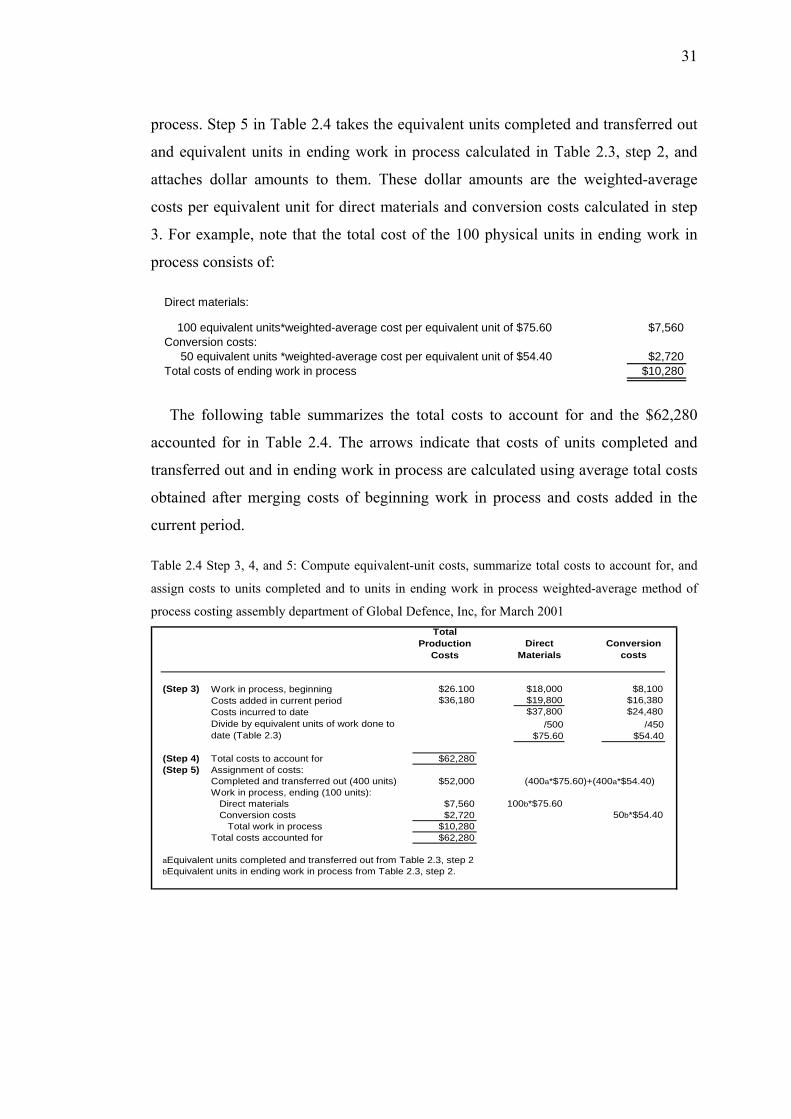
31
process. Step 5 in Table 2.4 takes the equivalent units completed and transferred out
and equivalent units in ending work in process calculated in Table 2.3, step 2, and
attaches dollar amounts to them. These dollar amounts are the weighted-average
costs per equivalent unit for direct materials and conversion costs calculated in step
3. For example, note that the total cost of the 100 physical units in ending work in
process consists of:
$7,560
$2,720$10,280Total costs of ending work in process
Direct materials:
100 equivalent units*weighted-average cost per equivalent unit of $75.60
50 equivalent units *weighted-average cost per equivalent unit of $54.40Conversion costs:
The following table summarizes the total costs to account for and the $62,280
accounted for in Table 2.4. The arrows indicate that costs of units completed and
transferred out and in ending work in process are calculated using average total costs
obtained after merging costs of beginning work in process and costs added in the
current period.
Table 2.4 Step 3, 4, and 5: Compute equivalent-unit costs, summarize total costs to account for, and
assign costs to units completed and to units in ending work in process weighted-average method of
process costing assembly department of Global Defence, Inc, for March 2001
(Step 3) $26.100 $18,000 $8,100$36,180 $19,800 $16,380
$37,800 $24,480/500
$75.60/450
$54.40
(Step 4) Total costs to account for $62,280(Step 5) Assignment of costs:
$52,000
$7,560 100b*$75.60$2,720 50b*$54.40
$10,280$62,280
aEquivalent units completed and transferred out from Table 2.3, step 2bEquivalent units in ending work in process from Table 2.3, step 2.
Work in process, beginning Costs added in current period Costs incurred to date Divide by equivalent units of work done to date (Table 2.3)
Completed and transferred out (400 units)
Total costs accounted for
Work in process, ending (100 units): Direct materials Conversion costs Total work in process
Total Production
CostsDirect
MaterialsConversion
costs
(400a*$75.60)+(400a*$54.40)
32
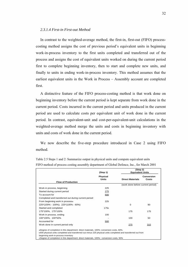
2.3.1.4 First-in First-out Method
In contrast to the weighted-average method, the first-in, first-out (FIFO) process-
costing method assigns the cost of previous period’s equivalent units in beginning
work-in-process inventory to the first units completed and transferred out of the
process and assigns the cost of equivalent units worked on during the current period
first to complete beginning inventory, then to start and complete new units, and
finally to units in ending work-in-process inventory. This method assumes that the
earliest equivalent units in the Work in Process – Assembly account are completed
first.
A distinctive feature of the FIFO process-costing method is that work done on
beginning inventory before the current period is kept separate from work done in the
current period. Costs incurred in the current period and units produced in the current
period are used to calculate costs per equivalent unit of work done in the current
period. In contrast, equivalent-unit and cost-per-equivalent-unit calculations in the
weighted-average method merge the units and costs in beginning inventory with
units and costs of work done in the current period.
We now describe the five-step procedure introduced in Case 2 using FIFO
method.
Table 2.5 Steps 1 and 2: Summarize output in physical units and compute equivalent units
FIFO method of process costing assembly department of Global Defence, Inc., for March 2001
(Step 1)
Physical Units Direct Materials
Conversion Costs
Flow of Production(work done before current period)
Work in process, beginning 225Started during current period 275To account for 500Completed and transferred out during current period:From beginning work in processa 225225*(100% - 100%); 225*(100% - 60%) 0 90Started and completed 175b
175*100%, 175*100% 175 175Work in process, ending 100100*100%; 100*50% - 100 50Accounted for 500Work done in current period only 275 315
aDegree of completion in this department: direct materials, 100%; conversion costs, 60%.b400 physical units completed and transferred out minus 225 physical units completed and transferred out frombeginning work-in-process inventorycDegree of completion in this department: direct materials, 100%; conversion costs, 50%
(Step 2)Equivalent Units

33
Step 1: Summarize the Flow of Physical Units. Table 2.5, step 1, traces the flow of
physical units of production. The following observations help explain the physical
units calculations.
The first physical units assumed to be completed and transferred out during
the period are the 225 units from the beginning work-in-process inventory.
Of the 75 physical units started, 175 are assumed to be completed. Recall
from the March data in Case 3 that 400 physical units were completed during
March. The FIFO method assumes that the first 225 of these units were from
beginning inventory; thus 175 (400 - 225) physical units must have been
started and completed during March.
Ending work-in-process inventory consists of 100 physical units – the 275
physical units started minus the 175 of these physical units completed.
Note that the physical units “to account for” equal the physical units
“accounted for” (500 units).
Step 2: Compute Output in Terms of Equivalent Units. Table 2.5 also presents the
computations for step 2 under the FIFO method. The equivalent-unit calculations for
each cost category focus on the equivalent units of work done in the current period
(March) only.
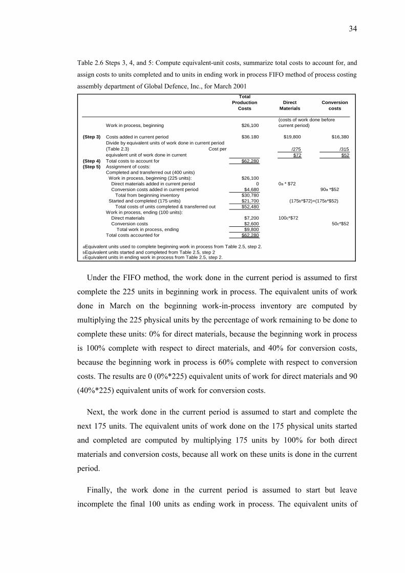
34
Table 2.6 Steps 3, 4, and 5: Compute equivalent-unit costs, summarize total costs to account for, and
assign costs to units completed and to units in ending work in process FIFO method of process costing
assembly department of Global Defence, Inc., for March 2001
Work in process, beginning $26,100
(Step 3) $36.180 $19,800 $16,380
/275 /315$72 $52
(Step 4) Total costs to account for $62,280(Step 5) Assignment of costs:
$26,1000 0a * $72
$4,680 90a *$52$30,780$21,700$52,480
$7,200 100c*$72$2,600 50c*$52$9,800
$62,280
cEquivalent units in ending work in process from Table 2.5, step 2.
Total costs of units completed & transferred out
Direct materials
Direct materials added in current period Conversion costs added in current period Total from beginning inventory Started and completed (175 units)
Total Production
CostsDirect
MaterialsConversion
costs
(175b*$72)+(175b*$52)
bEquivalent units started and completed from Table 2.5, step 2
(costs of work done before current period)
Work in process, ending (100 units):
Conversion costs Total work in process, ending
aEquivalent units used to complete beginning work in process from Table 2.5, step 2.
Costs added in current period Divide by equivalent units of work done in current period (Table 2.3) Cost per equivalent unit of work done in current
Completed and transferred out (400 units)
Total costs accounted for
Work in process, beginning (225 units):
Under the FIFO method, the work done in the current period is assumed to first
complete the 225 units in beginning work in process. The equivalent units of work
done in March on the beginning work-in-process inventory are computed by
multiplying the 225 physical units by the percentage of work remaining to be done to
complete these units: 0% for direct materials, because the beginning work in process
is 100% complete with respect to direct materials, and 40% for conversion costs,
because the beginning work in process is 60% complete with respect to conversion
costs. The results are 0 (0%*225) equivalent units of work for direct materials and 90
(40%*225) equivalent units of work for conversion costs.
Next, the work done in the current period is assumed to start and complete the
next 175 units. The equivalent units of work done on the 175 physical units started
and completed are computed by multiplying 175 units by 100% for both direct
materials and conversion costs, because all work on these units is done in the current
period.
Finally, the work done in the current period is assumed to start but leave
incomplete the final 100 units as ending work in process. The equivalent units of

35
work done on the 100 units of ending work in process are calculated by multiplying
100 physical units by 100% for direct materials (because all direct materials have
been added for these units in the current period) and 50% for conversion costs
(because 50% of conversion costs work has been done on these units in the current
period).
Step 3: Compute Equivalent-Unit Costs. Table 2.6 shows the step 3 computation
of equivalent-unit costs for work done in the current period only for direct materials
and conversion costs. For example, we divide current-period conversion costs of
$16,380 by current-period equivalent units for conversion costs of 315 to obtain cost
per equivalent unit of $52.
Step 4: Summarize Total Costs to Account For. The total production costs column
in Table 2.6 presents step 4 and summarizes the total costs to account for in March
2001 (beginning work in process and costs added in the current period) of $62,280,
as described in the example data.
Step 5: Assign Costs to Units Completed and to Units in Ending Work in Process.
Finally, Table 2.6 shows the step 5 assignment of costs under the FIFO method. The
costs of work done in the current period are first assigned to the additional work done
to complete the beginning work in process, then to the work done on units started
and completed during the current period, and finally to the ending work in process.
The easiest way to follow step 5 is to take each of the equivalent units calculated in
Table 2.5, step 3, and attach dollar amounts to them. The goal is to determine the
total cost of all units completed from beginning inventory and from work started and
completed in the current period, and the costs of ending work in process done in the
current period.
Only rarely is an application of pure FIFO ever encountered in process costing. As
a result, it should really be called a modified or departmental FIFO method, because
FIFO is applied within a department to compile the cost of units transferred out, but
the units transferred in during a given period usually are carried at a single average
unit cost as a matter of convenience. For example, the average cost of units
transferred out of the Assembly Department is $52,480/400 units = $131.20 per DG-

36
19 unit. The Assembly Department uses FIFO to distinguish between monthly
batches of production. The succeeding department, testing, however, costs these
units at one average unit cost ($131.20 in this illustration). If this averaging were not
done, the attempt to track costs on a pure FIFO basis throughout a series of processes
would be unduly cumbersome.
2.3.1.5 Comparison of Weighted-Average and FIFO Methods
The following table summarizes the costs assigned to units completed and to units
still in process under the weighted-average and FIFO process-costing methods for
our example:
FIFO(from Table 2.6) Difference
Cost of units completed and transferred out $52,480 (+)$480Work in process, ending $9,800 (-)$480Total cost accounted for $62,280$62,280
Weighted Average(from Table 2.4)
$52,000$10,280
The weighted-average ending inventory is higher than the FIFO ending inventory
by $480, or 4.9% ($480 / $9,800). This is a significant difference when aggregated
over the many thousands of products that Global Defence makes. The weighted-
average method in our example also results in lower cost of goods sold and hence
higher operation income and higher income taxes than does the FIFO method. There
are differences in equivalent-unit costs of beginning inventory and work done during
the current period account for the differences in weighted-average and FIFO costs.
Recall from the data that direct materials costs per equivalent unit in beginning work-
in process inventory is $80, and conversion costs per equivalent unit in beginning
work-in-process inventory is $60. These costs are greater than the $72 direct
materials and $52 conversion costs per equivalent unit of work done during the
current period. This reduction could be due to a decline in the prices of direct
materials and conversion cost inputs or could be a result of Global Defence
becoming more efficient.
For the Assembly Department, FIFO assumes that all the higher-cost units from
the previous period in beginning work in process are the first to be completed and

37
transferred out of the process, and ending work in process consists of only the lower-
cost current-period units. The weighted-average method however, smoothes out cost
per equivalent unit by assuming that more of the lower-cost units are completed and
transferred out, and some of the higher-cost units are placed in ending work in
process. Hence, in this example, the weighted-average method results in a lower cost
of units completed and transferred out and a higher ending work-in-process inventory
relative to FIFO.
Cost of units completed and hence operating income can differ materially between
the weighted-average and FIFO methods when the direct materials or conversion
costs per unit vary significantly from period to period, and the physical inventory
levels of work in process are large in relation to the total number of units transferred
out of the process. Thus, as companies move toward long-term procurement
contracts that reduce differences in unit costs from period to period, and reduce
inventory levels, the difference in cost of units completed under the weighted-
average and FIFO methods will decrease.
Managers need information from process-costing systems to aid them in pricing
and product-mix decisions and to provide them with feedback about their
performance. The major advantage of FIFO is that it provides managers with
information about changes in the costs per unit from one period to the next.
Managers can use this information to evaluate their performance in the current period
compared to a benchmark or compared to their performance in the previous period.
By focusing on and the costs of work done during the current period, the FIFO
method provides useful information for these planning and control purposes. The
weighted-average method merges unit costs from different periods and so obscures
period-to-period comparisons. The major advantages of the weighted-average
method, however, are its computational simplicity and its reporting of a more
representative average unit cost when input prices fluctuate markedly from month to
month.
Note that unlike in job-costing systems, activity-based costing has less
applicability in process-costing environments, because products are homogeneous
and hence use resources in a similar way. Furthermore, each process; assembly,

38
testing, and so on corresponds to the different activities. Managers reduce the costs
of activities by controlling the costs of individual processes.
2.3.1.6 Standard-Costing Method of Process Costing
As we have mentioned, companies that use process-costing systems produce
masses of identical or similar units of output. Setting standards for quantities of
inputs needed to produce output is often relatively straightforward in such
companies. Standard costs per input unit may then be assigned to these physical
standards to develop standard costs per output unit.
The weighted-average and FIFO methods become very complicated when used in
process industries that produce a wide variety of similar products. For example, a
steel-rolling mill uses various steel alloys produces sheets of various sizes and of
various finishes. Both the items of direct materials and the operations performed are
relatively few. But used in various combinations, they yield such a wide variety of
products that inaccurate costs for each product result if the broad averaging
procedure of actual process costing is used. Similarly, complex conditions are
frequently found, for example, in plants that manufacture rubber products, textiles,
ceramics, paints, and packaged food products. The standard-costing method of
process costing is especially useful in these situations.
Under the standard-costing method, teams of design and process engineers,
operations personnel, and management accountants determine separate standard or
equivalent-unit costs on the basis of the different technical processing specifications
for each product. Identifying standard costs for each product overcomes the
disadvantage of costing all products at a single average amount, as under actual
costing.
2.3.1.7 Transferred-In Costs in Process Costing
Many process-costing systems have two or more departments or processes in the
production cycle. As units move from department to department, the related costs are
also transferred by monthly journal entries. If standard costs are used, the accounting

39
for such transfers is relatively simple. However, if the weighted-average or FIFO
method is used, the accounting can become more complex. We now extend our
Global Defence, Inc., example to the Testing Department. As the assembly process is
completed, the Assembly Department of Global Defence immediately transfers DG-
19 units to its Testing Department. Here the units receive additional direct materials,
such as crating and other packing materials to prepare the units for shipment, at the
end of the process. Conversion costs are added evenly during the Testing
Department’s process. As units are completed in Testing, they are immediately
transferred to Finished Goods.
The following graphic summarizes these facts:
Transferred-in costs (also called previous department costs) are the costs incurred
in a previous department that are carried forward as the product’s cost when it moves
to a subsequent process in the production cycle. That is, as the units move from one
department to the next, their costs are transferred with them. Thus, computations of
Testing Department costs consist of transferred-in costs as well as the direct
materials and conversion costs added in Testing.
Transferred-in costs are treated as if they are a separate type of direct material
added at the beginning of the process. In other words, when successive departments
are involved, transferred units from one department become all or a part of the direct
materials of the next department; however, they are called transferred-in costs, not
direct materials costs.
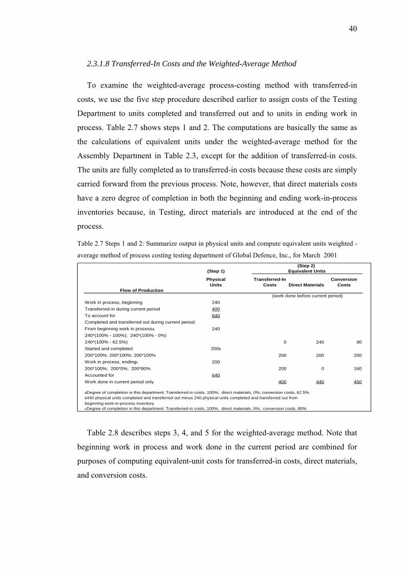
40
2.3.1.8 Transferred-In Costs and the Weighted-Average Method
To examine the weighted-average process-costing method with transferred-in
costs, we use the five step procedure described earlier to assign costs of the Testing
Department to units completed and transferred out and to units in ending work in
process. Table 2.7 shows steps 1 and 2. The computations are basically the same as
the calculations of equivalent units under the weighted-average method for the
Assembly Department in Table 2.3, except for the addition of transferred-in costs.
The units are fully completed as to transferred-in costs because these costs are simply
carried forward from the previous process. Note, however, that direct materials costs
have a zero degree of completion in both the beginning and ending work-in-process
inventories because, in Testing, direct materials are introduced at the end of the
process.
Table 2.7 Steps 1 and 2: Summarize output in physical units and compute equivalent units weighted -
average method of process costing testing department of Global Defence, Inc., for March 2001
(Step 1)
Physical Units
Transferred-In Costs Direct Materials
Conversion Costs
Flow of Production
Work in process, beginning 240Transferred-in during current period 400To account for 640Completed and transferred out during current period:From beginning work in processa 240240*(100% - 100%); 240*(100% - 0%)240*(100% - 62.5%) 0 240 90Started and completed 200b
200*100%; 200*100%; 200*100% 200 200 200Work in process, endingc 200200*100%; 200*0%; 200*80% 200 0 160Accounted for 640Work done in current period only 400 440 450
aDegree of completion in this department: Transferred-in costs, 100%; direct materials, 0%; conversion costs, 62.5%.b440 physical units completed and transferred out minus 240 physical units completed and transferred out frombeginning work-in-process inventorycDegree of completion in this department: Transferred-in costs, 100%; direct materials, 0%; conversion costs, 80%
(Step 2)Equivalent Units
(work done before current period)
Table 2.8 describes steps 3, 4, and 5 for the weighted-average method. Note that
beginning work in process and work done in the current period are combined for
purposes of computing equivalent-unit costs for transferred-in costs, direct materials,
and conversion costs.

41
Table 2.8 Steps 3, 4 and 5: Compute equivalent-unit costs, summarize total costs to account for, and
assign costs to units completed and to units in ending work in process weighted-average method of
process costing testing department of Global Defence, Inc, for March 2001
(Step 3) Work in process, beginning $51,600 $33,600 $0 $18,000$113,800 $52,000 $13,200 $48,600
$85,600 $13,200 $66,600
/640 /440 /600$133.75 $30 $111
(Step 4) Total costs to account for $165,400(Step 5) Assignment of costs:
$120,890
$26,750 200b*$133.750 0b*$30
$17,760 160b*$111$44,510
$165,400
bEquivalent units started and completed from Table 2.7, step 2aEquivalent units used to complete beginning work in process from Table 2.7, step 2.
Costs added in current period Costs
incurred to date Divide by
equivalent units of work done to date
(Table 2.7)
Completed and transferred out (440 units)Work in process, ending (200 units):
Total costs accounted for
(440a*$133.75) + (440a*$30) + (440a*$111)
Transferred-In Costs
Transferred-in costs Direct materials Conversion costs Total work in process, ending
Total Production
CostsDirect
MaterialsConversion
costs
2.3.1.9 Transferred-In Costs and FIFO Method
To examine the FIFO process-costing method with transferred-in costs, we again
use the five-step procedure. Table 2.9 shows steps 1 and 2. Other than considering
transferred-in costs, the computations of equivalent units are basically the same as
those under the FIFO method for the Assembly Department shown in Table 2.5.
Table 2.10 describes steps 3, 4, and 5. Note that the costs per equivalent unit for
the current period in step 3 are only calculated on the basis of costs transferred in and
work done in the current period. In steps 4 and 5, the total costs to account for and
accounted for of $165,880 under the FIFO method differ from the corresponding
amounts under the weighted-average method of $165,400 because of the different
costs of completed units transferred-in from the Assembly Department under the two
methods ($52,480 under FIFO and $52,000 under weighted average).

42
Table 2.9 Steps 1 and 2: Summarize output in physical units and compute equivalent units FIFO
method of process costing, testing department of Global Defence, Inc., for March 2001
(Step 1)
Physical Units
Transferred-In Costs Direct Materials
Conversion Costs
Flow of Production
Work in process, beginning 240Transferred-in during current period 400To account for 640Completed and transferred out during current period:From beginning work in processa 240240*(100% - 100%); 240*(100% - 0%)240*(100% - 62.5%) 0 240 90Started and completed 200b
200*100%; 200*100%; 200*100% 200 200 200Work in process, endingc 200200*100%; 200*0%; 200*80% 200 0 160Accounted for 640Work done in current period only 400 440 450
aDegree of completion in this department: Transferred-in costs, 100%; direct materials, 0%; conversion costs, 62.5%.b440 physical units completed and transferred out minus 240 physical units completed and transferred out frombeginning work-in-process inventorycDegree of completion in this department: Transferred-in costs, 100%; direct materials, 0%; conversion costs, 80%
(Step 2)Equivalent Units
(work done before current period)
Table 2.10 Steps 3, 4, and 5: Compute equivalent-unit costs, summarize total costs to account for, and
assign costs to units completed and to units in ending work in process FIFO method of process
costing, testing department of Global Defence, Inc., for March 2001.
Work in process, beginning $51,600(Step 3) $114,280 $52,480 $13,200 $48,600
/400 /440 /450
$131,20 $30 $108(Step 4) Total costs to account for $165,880(Step 5) Assignment of costs:
$51,6000 0a*$131.20
$7,200 240a*$30$9,720 90a*$108
$68,520$53,840
$122,360
$26,240 200c*$131.200 0c*$30
$17,280 160c*$108$43,520
$165,880
(200b*$131.20) + (200b*$30) + (200b*$108)
(costs of work done before current period)
bEquivalent units started and completed from Table 2.9, step 2
Work in process, ending (200 units):
Conversion costs Total work in process, ending
aEquivalent units used to complete beginning work in process from Table 2.9, step 2.
Completed and transferred out (440 units)
Total costs accounted for
Work in process, beginning (240 units):
Total Production
CostsDirect
MaterialsConversion
costsTransferred-In
Costs
cEquivalent units in ending work in process from Table 2.9, step 2.
Direct materials
Total costs of units completed and
Costs added in current period
Divide by equivalent units of work done in
current period (Table 2.3)
Cost per equivalent unit of work done in current
Transferred-in costs added in current period
Transferred-in costs
Direct materials added in current period Conversion costs added in current period Total from beginning inventory Started and completed (200 units)
43
Remember that in a series of interdepartmental transfers, each department is
regarded as being separate and distinct for accounting purposes. All costs transferred
in during a given accounting period are carried at one unit-cost figure, as described
when discussing modified FIFO, regardless of whether previous departments used
the weighted-average method or the FIFO method.
2.3.1.10 Common Mistakes with Transferred-In Costs
Here are some common pitfalls to avoid when accounting for transferred-in costs:
1. Remember to include transferred-in costs from previous departments in
your calculations.
2. In calculating costs to be transferred on a FIFO basis, do not overlook the
costs assigned at the beginning of the period to units that were in process
but are now included in the units transferred. For example, do not overlook
the $51,600 in Table 2.10.
3. Unit costs may fluctuate between periods. Therefore, transferred units may
contain batches accumulated at different unit costs. For example, the 400
units transferred in at $52.480 in Table 2.10 using the FIFO method
consists of when these units were worked on in the Assembly Department.
Remember, however, that when these units are transferred to the Testing
Department, they are cost at one average unit cost of $131.20 ($52,480/400)
as in Table 2.10.
4. Units may be measured in different terms in different departments.
Consider each department separately. For example, unit costs could be
based on kilograms in the first department and litres in the second
department. Accordingly, as units are received in the second department,
their measurements must be converted to litres.

44
2.3.2 Job Costing
In this system, the cost object is an individual unit, batch, or lot of a distinct
product or service called a job. The product or service is often custom-made, such as
specialized machinery made at Hitachi, construction projects managed by Bechtel.
Corporation, repairs jobs done at Sears Automotive Stores, and advertisements
produced by Saatchi and Saatchi. Each special machine made by Hitachi is unique
and distinct. Similarly an advertising campaign for one client at Saatchi and Saatchi
differs greatly from advertising campaigns for other clients. Because the products
and services are distinct, job costing systems can accumulate costs by each individual
product, service, or job.
Job order costing is fundamental to managerial accounting. It differs from Process
costing in that the flow of costs is traced by job instead of by process. For instance,
think of an assembly line making cookies. Job order costing would track how much
material is placed in each cookie. Process costing tracks the amount of dough used
the baking time, and other aspects of the process of making cookies. Job costing is
typically used for special orders or when the product made is unique. Process costing
is used when the products are more homogeneous in nature.
In a job costing system, costs are accumulated by job. For a typical job, direct
material and direct labour are tracked at their actual values. These are recorded and
tracked until the job is completed. Overhead is applied either by using a rate based
on direct labour hours, direct labour costs, direct material costs or by using an
Activity Based Costing (ABC) cost driver. In either case, once overhead is added, the
total cost for the job can be determined. Upon completion, the costs are transferred
out of Work in Process to Finished Goods (Cost of Goods Sold for service
industries).
2.3.2.1 Job Costing in Manufacturing
We illustrate job costing using the example of Robinson Company, which
operates at capacity to manufacture and install specialized machinery for the paper-
making industry at its Green Bay, Wisconsin, plant. In its job-costing system,

45
Robinson accumulates costs incurred on a job in all parts of the value chain-R&D,
design, manufacturing, marketing, distribution, and customer service. To make a
machine, Robinson procures some of the components from outside suppliers and
makes others itself. A key part of each of Robinson’s jobs is assembling and
installing the machine at customer sites; integrating it with the customer’s other
machines and processes, and ensuring its effective functioning.
The specific job we will focus on is the manufacture and installation of a small
pulp machine for Western Pulp and Paper Company in the year 2000, for a price of
$15,000. A key issue for Robinson in determining this price is the cost of doing the
job. Knowledge about its own costs helps Robinson price jobs to make a profit and to
make informed estimates of the costs of future jobs.
Consider Robinson’s actual costing system, a job-costing system that uses actual
costs to determine the cost of individual jobs. Actual costing is a method of a job
costing that traces direct costs to a cost object by using the actual direct-cost rate(s)
times the actual quantity of the direct-cost input(s) and allocates indirect costs based
on the actual indirect-cost rate(s) times the actual quantity of the cost-allocation
base(s).
2.3.2.2 General Approach to Job Costing
We present a seven-step procedure to assign actual costs to individual jobs. This
procedure applies equally to job costing in the manufacturing, merchandising, and
service sectors.
Step1. Identify the Chosen Cost Object(s): The cost object in the Robinson
Company example is Job Number WPP 298, manufacturing a pulp machine for the
Western Pulp and Paper Company in the year 2000.
Step2. Identify the Direct Costs of the Job: Robinson identifies two direct
manufacturing cost categories – direct materials and direct manufacturing labour.
Direct materials costs for the Western Pulp and Paper Company job are $4,606,
while direct manufacturing labour costs are $1,579.

46
Step3. Select the Cost-Allocation Base(s) to use for Allocating Indirect Costs to
the Job: Indirect manufacturing costs are costs that cannot be traced to specific jobs.
Yet completing various jobs would be impossible without incurring indirect costs
such as supervision, manufacturing engineering, utilities and repairs. These costs
must be allocated to jobs. Different jobs require different quantities of indirect
resources. The objective of allocating indirect costs is to measure the underlying
usage of indirect resources by individual jobs.
Robinson chooses direct manufacturing labour-hours as the only allocation base
for linking all indirect manufacturing costs to jobs, since Robinson believes that
direct manufacturing labour-hours measures how individual jobs use manufacturing
overhead resources, such as salaries paid to supervisors, engineers, production
support staff, and quality management staff. There is a strong cause-and-effect
relationship between the indirect manufacturing resources demanded and the direct
manufacturing labour-hours required by individual jobs. In the year 2000, Robinson
records 27,000 actual direct manufacturing labour-hours.
Step4. Identify the Indirect Costs Associated with Each Cost-Allocation Base:
Because Robinson believes that a single cost-allocation base, direct manufacturing
labour-hours, can be used to allocate indirect manufacturing costs to products, it
creates a single cost pool called manufacturing overhead costs. This pool represents
the indirect costs of the Green Bay Manufacturing Department that are difficult to
trace directly to individual jobs. In 2000, actual indirect manufacturing costs total
$1,215,000.
Step5. Compute the Rate Per unit of Each Cost-Allocation Base Used to
Allocate Indirect Costs to the Job: For each cost pool, the indirect-cost rate is
calculated by dividing total overhead costs in the pool by the total quantity of the
cost-allocation base. Robinson calculates the allocation rate for its single
manufacturing overhead cost pool as follows:

47
cos coscoscos
$1,215,00027,000$45
Actual total ts in indirect t poolActual indirect t rateActual total quantity of t allocation base
direct manufacturing labour hoursper direct manufacturing labour hour
−− =
−
=−
= −
Step6. Compute the Indirect Costs Allocated to the Job: The indirect costs of a
job are computed by multiplying the actual quantities of the different allocation bases
(one for each cost pool) used to complete a job by their respective indirect cost rates.
To make the pulp machine, Robinson uses 88 direct manufacturing labour-hours, the
cost-allocation base for its only indirect-cost pool. Indirect costs allocated to the pulp
machine job equal $3,960 ($45 per direct manufacturing labour-hour*88 hours).
Step7. Compute the Total Cost of the Job by Adding All Direct and Indirect
Costs Assigned to It: The cost of the pulp machine job for Western Pulp is $10,145.
$4,606$1,579 $6,185
$3,960$10,145
Indirect manufacturing costs ($45*88 direct manufacturing labour-hours) Total manufacturing costs of job
Direct manufacturing costs Direct materials Direct manufacturing labour
Recall that Robinson was paid $15,000 for the job. Thus, the actual costing
system shows a gross margin of $4,855 ($15,000-$10,145) and a gross margin
percentage of 32.37% ($4,855÷$15,000).
Robinson can use the gross margin and gross margin percentage calculations to
compare profitability across various jobs and identify the most profitable types of
jobs for its sales force to target. At the same time, Robinson can examine the reasons
why some jobs show low profitability. Job cost analysis provides crucial information
for judging performance and making future improvements.

48
Figure 2.5 Job-costing overview for determining the manufacturing costs of jobs’ at Robinson Co.
Figure 2.5 presents an overview of the Robinson Company job-costing system.
This exhibit includes the five building block concepts-cost object, direct costs of a
cost object, indirect costs of a cost object, cost pool, and cost-allocation base.
Costing-system overviews like Figure 2.5 are important learning tools. We urge you
to sketch one when you need to understand a costing system in manufacturing,
service, or merchandising companies. Note the correspondence between the figure
diagram and the cost of the pulp machine job described in step7. Figure 2.5 shows
two direct-cost categories (direct materials and direct manufacturing labour) and one
indirect-cost pool (manufacturing overhead) used to allocate indirect costs. The costs
in step7 also have three dollar amounts that correspond to two direct and one indirect
cost categories.

49
2.3.2.3 Two Major Cost Objects: Products and Departments
As determined, all costs are recorded to help individuals make decisions. Cost
objects are chosen to aid decision making. The Figure 2.5 overview focuses on one
major cost object of an accounting system: products. Managers also focus on a
second major cost object: responsibility centres, which are parts, segments, or
subunits of an organization whose managers are accountable for specified sets of
activities. Examples are departments, groups of departments, divisions, or geographic
territories. Manufacturing job-costing system assign costs first to responsibility
centres and then to jobs.
The most commonly encountered responsibility centre is a department.
Identifying department costs helps managers to control costs for which they are
responsible. It also enables senior management to evaluate the performance of
subordinates and the performance of subunits of the organization as economic
investments. For example, Robinson identifies manufacturing as a critical activity
and the Manufacturing Department as an important cost object. The costs of the
Manufacturing Department include all costs of materials; manufacturing labour; and
other manufacturing costs such as supervision, engineering, and production and
quality control.
Note especially that costs such as supervision, engineering, and production and
quality control that were considered indirect or overhead costs when costing
individual jobs are direct costs of the Manufacturing Department since although
these costs are difficult to trace to individual jobs within the Manufacturing
Department in an economically feasible way, they are easily identified with and
traced to the Manufacturing Department itself.
2.3.2.4 Time Period Used to Compute Indirect-Cost Rates
Robinson Company computes indirect-costs rates in step 5 on the basis of an
annual period. If it used weekly or monthly rates, Robinson would be able to
calculate actual costs of jobs much earlier and not have to wait until the end of the

50
year. There are two important reasons for using longer time periods to calculate
indirect-cost rates.
1. The numerator reason (indirect cost pool): The shorter the period, the greater
the influence of seasonal patterns on the level of costs. For instance, if indirect-
cost rates were calculated each month, costs of heating (including in the
numerator) would be charged only to winter production. The use of an annual
period incorporates the effect of all four seasons into a single indirect-cost rate.
Levels of total indirect costs are also affected by no seasonal erratic costs.
Examples include costs incurred in a particular month that benefit operations
during future months: repairs and maintenance of equipment, and vacation and
holiday pay. If monthly indirect-cost rates were counted, jobs done in a month
with high no seasonal erratic costs would be loaded with these costs.
2. The denominator reason (quantity of the allocation base): Another rationale
for longer periods is the need to spread monthly fixed indirect costs over
fluctuating levels of output. Some indirect costs may be variable with respect to
the cost-allocation base, whereas other indirect costs are fixed.
Suppose a company schedules its production to correspond with a highly seasonal
sales pattern. Assume the following mix of variable indirect costs (such as supplies,
repairs and indirect manufacturing labour) and fixed indirect costs (plant
depreciation and engineering support):
Variable Fixed Total
1 2 3
High-output month $40.000 $60.000 $100.000 3.200 $31.25
Low-output month 10.000 60.000 70.000 800 $87.50
Allocation Rate Per Direct
Manufacturing Labour-Hour
(5)=(3):(4)
Indirect Costs Direct Manufacturing Labour-Hours
(4)
Note that the variable indirect costs change in proportion to changes in direct
manufacturing labour-hours. Therefore, the variable indirect-cost rate is the same in
both the high-output and low-output months ( )$40,000 3200 $12.50; $10,000 800 $12.50÷ = ÷ = .

51
Because of the fixed costs of 60,000, monthly total indirect-cost rates vary sizably-
from $31.25 per hour to $87.50 per hour. Few managers believe that identical jobs
done in different months should be allocated indirect-cost charges per hour that differ
so significantly ($87.50:$31.25=280%). In our example, management has committed
itself to a specific level of capacity far beyond a mere 30 days per month. An
average, annualized rate based on the relationship of total annual indirect costs to the
total annual level of output will smooth out the effect of monthly variations in output
levels.
2.3.3 Normal Costing
The difficulty of calculating actual indirect-cost rates on a weekly or monthly
basis means that managers cannot calculate the actual costs of jobs as they are
completed. Managers often want a close approximation of the manufacturing costs of
various jobs on a timely basis, not just at the end of the year. Managers want these
costs for various ongoing uses, including choosing which job to emphasize or
deemphasize, pricing jobs, managing costs, and preparing interim financial
statements. Because management benefits form having immediate access to the costs
of jobs, few companies wait until the actual manufacturing overhead is finally
known before allocating overhead costs in computing the costs of jobs. Instead, a
predetermined or budgeted indirect-cost rate is calculated for each cost pool at the
beginning of a fiscal year, and overhead costs are allocated to jobs as work
progresses. For the numerator and denominator reasons described in the preceding
section, the budgeted indirect-cost rate is computed for each cost pool using the
budgeted annual indirect cost and the budgeted annual quantity of the cost-allocation
base. The use of budgeted indirect-cost rates gives rise to normal costing.
Normal costing is a costing method that traces direct costs to a cost object by
using the actual direct-cost rate(s) times the actual quantity of the direct-cost input(s)
and allocates indirect costs based on the budgeted indirect-cost rate(s) times the
actual quantity of the cost-allocation base(s). Note that both actual costing and
normal costing trace direct costs to jobs in the same way. The actual quantities and
actual rates of direct materials and direct manufacturing labour used on a job are
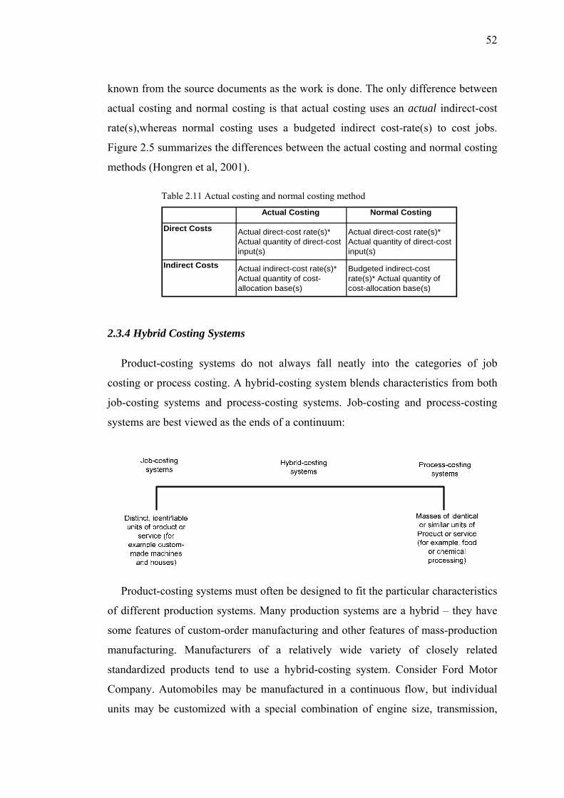
52
known from the source documents as the work is done. The only difference between
actual costing and normal costing is that actual costing uses an actual indirect-cost
rate(s),whereas normal costing uses a budgeted indirect cost-rate(s) to cost jobs.
Figure 2.5 summarizes the differences between the actual costing and normal costing
methods (Hongren et al, 2001).
Table 2.11 Actual costing and normal costing method
Actual Costing Normal Costing
Direct Costs Actual direct-cost rate(s)* Actual quantity of direct-cost input(s)
Actual direct-cost rate(s)* Actual quantity of direct-cost input(s)
Indirect Costs Actual indirect-cost rate(s)* Actual quantity of cost-allocation base(s)
Budgeted indirect-cost rate(s)* Actual quantity of cost-allocation base(s)
2.3.4 Hybrid Costing Systems
Product-costing systems do not always fall neatly into the categories of job
costing or process costing. A hybrid-costing system blends characteristics from both
job-costing systems and process-costing systems. Job-costing and process-costing
systems are best viewed as the ends of a continuum:
Product-costing systems must often be designed to fit the particular characteristics
of different production systems. Many production systems are a hybrid – they have
some features of custom-order manufacturing and other features of mass-production
manufacturing. Manufacturers of a relatively wide variety of closely related
standardized products tend to use a hybrid-costing system. Consider Ford Motor
Company. Automobiles may be manufactured in a continuous flow, but individual
units may be customized with a special combination of engine size, transmission,

53
music system, and so on. Companies develop hybrid-costing systems in such
situations. The concepts in Action feature describe the evolution of a hybrid-costing
system.

54
CHAPTER THREE
ACTIVITY-BASED COSTING ANALYSIS
Gradually, managerial accountants have become aware of the vanishing relevance
of the numbers they produce for end-users and decision makers. In 1994, Professor
John K. Shank of Dartmouth College said at the Institute of Management
Accountants’ 75th Anniversary Conference in New York City: “Traditional
accounting is at best useless, and at worst dysfunctional and misleading”. Those are
pretty strong words. The audience was silent. But Shank continued to describe the
imminent “sea change” that will occur in managerial accounting. He described how
cost management will be to the 1990s what total quality management was to the
1980s (Cokins, 1996).
Activity-based costing (ABC) is part of that sea change. ABC is not a replacement
for the traditional general ledger accounting. Rather, it is a translator or overlay, as
Figure 3.1, that lies between the cost accumulators or the expenditure account
balances in the general ledger and the end-users who apply cost data in decision
making. ABC converts inert cost data into relevant information so that the users can
take action (Cokins, 1996).
Figure 3.1 ABC/ABM reassign costs
54

55
ABC initially captured managements’ attention in the early 1980s as a superior
product and service costing technique. ABC removed the grotesquely distorting
effect of broad-brushed overhead allocators, like labour hours or sales dollars. It
replaced cost allocations with substantially more realistic cost assignments and
consequently much greater accuracy. Then, in the 1990s, managers discovered that
the same data they generated to recompute their ABC product or service costs could
also be used to gain better insights and manage their product design and process
design costs. It could also be used for performance measurements that align with
business processes.
ABC is becoming increasingly more important for both identifying improvement
opportunities and measuring the realized benefits of performance initiatives on an
after-the-fact basis. Today’s traditional costing practices show very little about the
costs of cross-functional business processes and even less about where the non-
value-added costs are. Further, when asked to detail their actual cost savings or cost
avoidance realized from a project, managers cannot adequately do so.
Beyond thinking of ABC as a much better costing tool is recognizing it as truly an
organizational methodology. Senior managers have been frustrated by the difficulties
in bringing about change within their organization, and ABC data is paying an
important role with it.
This chapter will present the philosophy, implementation steps, calculation
methodology and some success/failure factors of implementing ABC.
3.1 History of Activity Based Costing
Traditionally cost accountants had arbitrarily added a broad percentage of
expenses onto the direct costs to allow for the indirect costs.
However as the percentages of indirect or overhead costs had risen, this technique
became increasingly inaccurate because the indirect costs were not caused equally by
all the products. For example, one product might take more time in one expensive
machine than another product, but since the amount of direct labour and materials
56
might be the same, the additional cost for the use of the machine would not be
recognized when the same broad 'on-cost' percentage is added to all products.
Consequently, when multiple products share common costs, there is a danger of one
product subsidizing another.
The concepts of ABC were developed in the manufacturing sector of the United
States during the 1970s and 1980s. During this time, the Consortium for Advanced
Management-International, now known simply as CAM-I, provided a formative role
for studying and formalizing the principles that have become more formally known
as Activity-Based Costing.
Robin Cooper and Robert S. Kaplan, proponent of the Balanced Scorecard,
brought notice to these concepts in a number of articles published in Harvard
Business Review beginning in 1988. Cooper and Kaplan described ABC as an
approach to solve the problems of traditional cost management systems. These
traditional costing systems are often unable to determine accurately the actual costs
of production and of the costs of related services. Consequently managers were
making decisions based on inaccurate data especially where there are multiple
products.
Instead of using broad arbitrary percentages to allocate costs, ABC seeks to
identify cause and affect relationships to objectively assign costs. Once costs of the
activities have been identified, the cost of each activity is attributed to each product
to the extent that the product uses the activity. In this way ABC often identifies areas
of high overhead costs per unit and so directs attention to finding ways to reduce the
costs or to charge more for costly products.
Activity-based costing was first clearly defined in 1987 by Robert S. Kaplan and
W. Bruns as a chapter in their book Accounting and Management: A Field Study
Perspective. They initially focused on manufacturing industry where increasing
technology and productivity improvements have reduced the relative proportion of
the direct costs of labour and materials, but have increased relative proportion of
indirect costs. For example, increased automation has reduced labour, which is a
direct cost, but has increased depreciation, which is an indirect cost.

57
Like manufacturing industries, financial institutions also have diverse products
and customers which can cause cross-product cross-customer subsidies. Since
personnel expenses represent the largest single component of non-interest expense in
financial institutions, these costs must also be attributed more accurately to products
and customers. Activity based costing, even though originally developed for
manufacturing, may even be a more useful tool for doing this.
3.2 Definition of Activity Based Costing
The overarching issue with ABC/ABM involves its perception as just another way
to spin financial data rather than its use as mission-critical managerial information.
The Information Age we are entering can be mind-boggling. In our future, as
technology advances, so will the demand to access massive amounts of relevant
information. The companies and organizations that survive will be those that can
answer these questions (Cokins, 1996):
“How do we access all this data?”
“What do we do with it?”
“How do we shape the data and put into a form with which we can
work?”
“What will happen when we apply technologies developed during the
Information Age?”
Clearly, as information technology evolves, organizations will increase their
effectiveness. Further, as markets change, companies and organizations will run into
global competitors that increasingly look to information and information technology
for competitive advantage. ABC/ABM is involved in this broad arena of
“outsmartsmanship.”
What are today’s burning issues with implementing ABC/ABM? The answers
depend on the starting point of an organization. There appear to be three sequenced
starting points: (1) one for beginners, (2) one for pilots, and (3) one for advanced,
mature users. Each starting point is unique and discussed below.

58
1. Since the late 1980s, the concepts of ABC/ABM have been sufficiently
explained in seminars and published articles; by now most financial managers
and many operations personnel adequately understand what ABC/ABM is.
That is not the problem anymore for organizations waiting to begin
implementation of ABC/ABM. The beginners’ key issue today is how to get
started. Their employees intuitively feel that their financial reporting both
blocks the view of true costs across business processes as well as distorts
product and service costs. In sum, employees have few reliable facts, severely
inaccurate product and service costs, and little true cost visibility. Beginner
organizations can’t get started on ABC/ABM for a variety of reasons,
including some users’ fear of accountability as well as misconceptions that
ABC/ABM involves a mud slide of data with horrendous updating and
reporting problems.
2. The issue with the ABC/ABM pilot starting point involve avoiding
implementation failure. Over these past few years, the jungle drums have
been beating between other companies describing the lack of success with
ABC/ABM, and consequently, newly formed project teams are cautious.
Companies that have ventured into an ABC/ABM pilot are motivated to
move away from their traditional cost system and the bad decisions it is
causing; but they also appreciate that when they do change, there are
preventions they can take to assure a successful implementation.
3. The third starting point is that of the advanced, mature users. These
companies usually have two or more pilots that have been in progress for well
over a year. They are moving toward wide employee acceptance of his new
form of financial data and increasing user for more frequent reporting, for
selective greater detail, or for integration with other application software
systems, like their customer order quotation systems, which are still
harnessed to the old, flawed traditional cost data. The advanced users’ key
issue is how to migrate from their PC-based models that take periodic cost
snapshots to a permanent, fully-integrated production ABC/ABM system.

59
This is no small task because the pilots were championed by strong “pioneer-
types” of individuals who raced the clock to maintain momentum and left
little documentation behind when implementing their pilot. A permanent
ABC/ABM production system must be repeatable and reliable, and this
involves technical information systems personnel and their end-users, who
we can refer to as the “settlers”. Settlers like predictability and consistency.
Settlers often feel like they are left behind to clean up the mess the pioneers
created before they moved on to system integration of ABC/ABM.
Figure 3.2 Three starting points for ABC/ABM
Regardless of a company’s starting point with ABC/ABM, much more attention
must be placed on stimulating the no accountants and end-users to buy into
ABC/ABM concepts and data.
Jonathan B. Schiff, former editor of the Cost Management Group of the Institute
of Management Accountants (IMA) monthly Cost Management Update, summarized
ABC’s take-off problem in the November 1993 issue. He described the acceptance of
ABC/ABM as an imbalance between the supply and demand sides of an equation.
The substantial increase in ABC/ABM training and development programs, mainly
directed to finance and accounting managers, represents a hefty supply side of
equation.

60
The demand side is the active stimulation of internal end-users to apply
ABC/ABM information in their decisions and analyses. This has been weak. Without
end-user interest on the demand side, the upgraded supplier will have difficulty
integrating the new information into the end users’ decision-making habits. If there is
not a healthy relationship between the accountants and their internal customers, then
merely upgrading the supply side could have a negligible effect on improving he
organization’s decision-making capabilities.
End users will assume no change, resulting in the same outputs as in the past –
information that is late, difficult to understand, inaccurate, confusing, and overly
complex.
The shame is it is only through the application of ABC/ABM technology, not the
technology itself, that we get the full impact of any investment in better cost
management techniques and information. One can only create value for customers by
applying ABC/ABM.
Simply put, ABC/ABM has two groups operating too much in isolation from the
other: The inventors and the end-users of the ABC/ABM technology. The end-users
do not believe that the inventors understand their problem. And the inventors believe
they are solving the end-users’ problem. One possesses the need, while the other
possesses the technology and know-how. This gap in communications, knowledge,
and understanding must and will be closed through better collaboration.
In summary, there is no lack of issues for the ABC/ABM movement. The
ABC/ABM method is certainly more correct than the traditional accounting
system’s: but there is so much more involved in creating wide acceptance and
deploying its information.
3.2.1 Popular Business Improvements Approaches
Today organizations want business improvement programs that create value and
ultimately bring profits to the bottom line. They want to convert carbon-based coal
into diamonds. Companies appear less interested in improvement programs that are

61
only value-enabling, and that only locate carbon. They want to value-creating
programs.
Figure 3.3 lists five of the most popular business improvement approaches that
many companies today are consciously or subconsciously applying. The diagram
simply shows a corrective performance feedback loop that starts and ends with
customers. It reveals that organizations try to focus their “4M” resources (manpower,
machines, money and materials) to produce desired results while constantly
overcoming obstacles and organizational residence.
Figure 3.3 Five popular approaches to Business Improvement (Cokins, 1996)

62
The five popular business improvement methods are as follows:
Method Premise Thought Leader/Organization
The learning organization
Core competencies
Organizational Behaviour
Process Improvement
People matter. Really matter. Resistance of change, incentives, and empowerment is not fluff
We compete on knowledge and speed of organizational learning is critical
Peter Senge, Massachusetts Instute of Technology
Time-based and total quality management Noncomformance to achievable
plans erodes performance
Gearge Stalk, Boston Consulting Group, and Dr. W. Edwards Deming
Superior processes provide longer-sustaining competitive advantages than do products. Be innnovative.
Michael Hammer, formerly Massachusetts Institute of Technology
Deal from your market-critical strengths, and outsource your less critical weakness
C.K. Prahalad, University of Michigan, and Gary Hamel, London Business
Chris Argris, Harvard Business School
Although ABC/ABM can serve as “initiative accelerators” to all five methods, its
largest impact is on the last two. With regard to change management, ABC/ABM
presents emotionally compelling facts that stimulate workers to want to change the
way things are with regard to process improvement, ABC/ABM quantifies the
business process across the organizations and highlights where the waste or
opportunities are located.
One of the five methods described above combines total quality management
(TQM) and cycle-time reduction. The prevailing logic with this form of
improvement program has been that if you improve quality or reduce lead time, you
effectively are removing waste, error, and low value-adding work content – and
therefore costs will take care of themselves. That logic is now being challenged in
some circles, but debuting managerial philosophies can be like religious wars.
ABC/ABM can help make good on some of the failed promises about TQM and JIT
improvement programs.
A common employee complaint concerns the “program-of-the-month” approach
that is, following management fads with negligible long-term impact. Management’s

63
dilemma involves a trade-off: A company must be do lots of good things
simultaneously, but organizations also have a natural tendency to lose focus.
Therefore, organizations need guidance and reinforcements of specific direction
through periodic programs to emphasize something important; but, in the long run,
everything is connected to everything. Management can prioritize what to work on
that ABC/ABM can help.
Simply put, ABC/ABM is a tool, not a solution. It brings visibility of the
symptoms of problems from which effective solutions can be inferred. In some cases,
ABC/ABM brings visibility to that which has never been seen before; in other cases,
it replaces existing flawed and highly misleading cost data caused by bad and
distorting allocations. ABC/ABM has four objectives:
a) To eliminate or minimize low value adding cost.
b) To introduce efficiency and effectiveness and thus streamline the value-
adding activities that is executed in business processes to improve the yield.
c) To find the root causes of problems and correct them. Remember, costs are
a symptom.
d) To remove distortions caused by poor assumptions and bad cost allocations.
Regardless of the performance improvement methods and tools that companies
choose to apply, they should be aware of that their enterprises are subject to certain
natural properties, just like we are subject to physical laws of the universe such as
gravity and the speed of light. One commonly overlooked natural property of
business is that time, cost, and quality are linked, not independent of one another. All
improvement efforts, continuous or breakthrough, are intended to increase value for
one or more stakeholders. The goal is more efficient responsiveness with profit.
Today’s managers are recognizing how systematic and interconnected their work
is. That is one reason team-based managing has become so popular. There are no
more “island solutions”. Businesses today must simultaneously behave better, faster,
and cheaper – quality, time, and cost. No more can companies pick two and let third
one slide. They have to consider the three elements all together. There must be
integration.
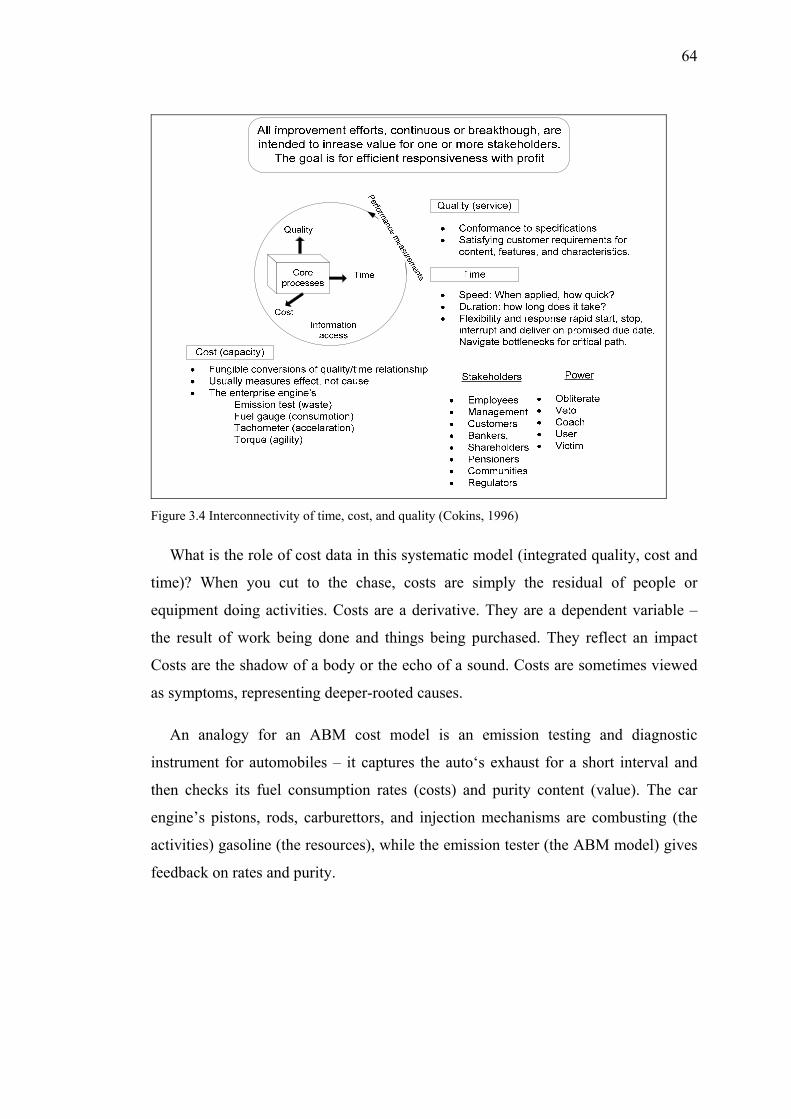
64
Figure 3.4 Interconnectivity of time, cost, and quality (Cokins, 1996)
What is the role of cost data in this systematic model (integrated quality, cost and
time)? When you cut to the chase, costs are simply the residual of people or
equipment doing activities. Costs are a derivative. They are a dependent variable –
the result of work being done and things being purchased. They reflect an impact
Costs are the shadow of a body or the echo of a sound. Costs are sometimes viewed
as symptoms, representing deeper-rooted causes.
An analogy for an ABM cost model is an emission testing and diagnostic
instrument for automobiles – it captures the auto‘s exhaust for a short interval and
then checks its fuel consumption rates (costs) and purity content (value). The car
engine’s pistons, rods, carburettors, and injection mechanisms are combusting (the
activities) gasoline (the resources), while the emission tester (the ABM model) gives
feedback on rates and purity.

65
3.2.2 The Emerging Consensus on ABC/ABM
ABC/ABM data are currently not being used as a managerial command-and-
control tool. In fact, this is quite the opposite. The most popular uses of the new
financial data involve forward planning and predictive modelling of the cost impact
of decisions that will affect the future. Rarely is ABC/ABM data used with an
“accounting police” mentality in a similar way that standard cost and budget variance
data and analyses are frequently used to curb department spending and punish
irresponsible spenders. ABC/ABM enhances the new image of financial accountants
as partners, not enforces and gatekeepers, with sales and operations personnel in
navigating and coordinating the various business improvement program options and
initiatives.
3.2.2.1 Cost of Processes (ABM)
The bulleted items below will read like sound bites. They are written more for
quick overview than for depth.
• As organizations flatten in structure and companies strengthen their
commitment to customer satisfaction and customer retention, business
processes are becoming more visible. Business processes run across artificial
organizational boundaries, and they are emerging in full view of all managers’
eyes as the vehicles that bring and achieve value for customers. Some business
processes are part of the supplier value chain. The supply chain is what needs
to be better managed. Activity accounting quantifies this new view with cost
data.
• Customers are gaining in power. Brand loyalty is declining and giving way to
everyday low prices and a keener sense for value. Customers are also seeking
increased customization to meet their unique needs. There is no “average”
customer. This creates greater product variety and diversity along with new
services. Business is no longer some sort of anonymous distribution system
through which to pump products.

66
• Organizations are discovering that the business process performance levels
necessary to remain competitive exceed what is possible from conventional,
highly vertical, functional organization forms. The traditional corporate model
is becoming less valid as business processes transcend the old departmental
boundaries. Future cost reductions and performance improvements can be
achieved only through reconfiguring work activities into fewer, more integrated
jobs. Optimizing a functional department is no optimal.
• The major, core cross-functional business processes of any organization are
large in size and few in number. Examples of business processes are order
fulfilment (from customer order to cash payment) or new product development
(from concept idea to final prototype).
• Functional names, like an Order Entry Department, disguise the broader
business processes. In contrast, groups of activities, like those occurring in
search and development, are often not recognized as core business processes.
• Customers see increasing value in good business processes and will pay a
premium for them. For example, Federal Express overnight delivery and
McDonald’s ready-to-serve meals revolutionized their industries.
• Traditional financial accounting supports old-fashioned functional thinking.
When you tilt the organization sideways 90 degrees and begin thinking in terms
of process and not function, then the financial accounting system becomes an
obstacle. Here are the two major problems:
The chart-of-accountants (wages, fringe benefits, supplies, etc.) gives
no visibility to work, to work’s content, and to work’s worth to
customers. To overcome this deficiency, activity accounting forces the
use of verb-noun grammar so that employees can finally see the work –
and employees are actually more comfortable with this more natural
language of activities.
Departmental or cost centre segmented financial reporting perpetuates
the vertical hierarchy as the driving force in an organization, instead of

67
the more deserving customer who is at the end of a business process
crossing the organization horizontally.
• A significant challenge will surface as process-based cost reporting and
associated performance measures take root. There will be tension between
those who will continue to support functional organizational goals and those
wishing to meet customer needs. In many organizations the neighbours don’t
true one another. In customer-focused companies, they behave like a unified
community.
• Traditional accounting blocks managers from seeing, understanding, and
reacting to the costs they should be managing. It blocks them from
understanding the causes of their costs. In contrast, activity accounting brings
visibility. It also brings quantification. ABC/ABM connects action words to
management concepts and vice versa. It shows end-users where
accountability and empowerment intersect. It is a mirror reflection of the
organization’s costs of business processes.
• Both processes owners and participants will need cost data that support this
new end-to-end horizontal thinking. New organizational alignments to
support customers will exhibit centralized control with decentralized
execution. The former requires better cost planning; the latter, more relevant
cost monitoring.
• Activity accounting provides a natural framework to assign value. Where are
we adding value? Where are we not adding value? How well are we adding
value? These questions can be answered by scoring or grading the value-
content of individual activities within supply chain processes.
• Total quality management (TQM) teams and just-in-time (JIT) cycle-time
compression teams are taught to think in terms of processes and to measure
processes. With some outdated business processes, encrusted with a legacy of
path-dependent, quick-fix corrections, TQM and JIT teams are now running
into walls, namely themselves. Their efforts are not always turning into

68
benefits or improving profits. Senior management is getting disturbed by the
diminishment of benefits realized from TQM.
• Why examine activities? Examining activities helps employees understand
activities. Also, the root causes that drive activity costs can be identified and
included in employees” thinking. This is all very human and behavioural.
Remember that activities ultimately always involve people serving other
people. The idea is to positively influence behaviour. And that means not
penalizing people for errors, but discouraging them from the repetition of
errors.
Only activity-based accounting principles support process-based thinking and its
associated business improvement actions and programs. Activities are such a central
foundation. TQM is doing activities without errors. JIT is doing activities without
waste. Reengineering is synchronizing activities across functional boundaries. With
traditional accounting there is no process view; you can get there from here. With
activity accounting you can follow the path of a business process. Also, you can
check the alignment of costs with senior management’s defined strategies.
3.2.2.2 Product and Service Costs (ABC)
While allocations are out, direct costing is in:
• Complexity and product/service diversity are escalating. Unique customer
needs are driving this explosion. Meeting customer needs is resulting in
increasing overhead costs can be casually traced to whom (which customer)
or to what (which product) the overhead activity work is benefiting. When
redistributing costs, accountants call whom and what final cost objects.
• Ideally, all costs should be directly charged, but as technology increases,
more costs are indirect. Activity-based costing acts as a surrogate for directly
charging costs of activities that traditionally have not been traced to cost
objects. ABC displaces the traditional and distorting practice of allocating
expenses. Allocations should be a last resort.
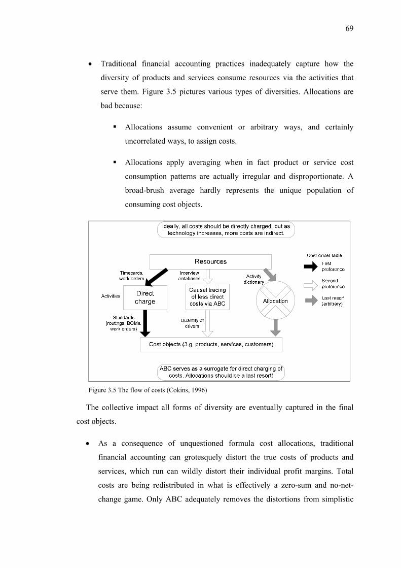
69
• Traditional financial accounting practices inadequately capture how the
diversity of products and services consume resources via the activities that
serve them. Figure 3.5 pictures various types of diversities. Allocations are
bad because:
Allocations assume convenient or arbitrary ways, and certainly
uncorrelated ways, to assign costs.
Allocations apply averaging when in fact product or service cost
consumption patterns are actually irregular and disproportionate. A
broad-brush average hardly represents the unique population of
consuming cost objects.
Figure 3.5 The flow of costs (Cokins, 1996)
The collective impact all forms of diversity are eventually captured in the final
cost objects.
• As a consequence of unquestioned formula cost allocations, traditional
financial accounting can grotesquely distort the true costs of products and
services, which run can wildly distort their individual profit margins. Total
costs are being redistributed in what is effectively a zero-sum and no-net-
change game. Only ABC adequately removes the distortions from simplistic

70
cost allocations. An allocation-free cost system is like a smoke-free
environment – no pollution. In short, don’t allocate – prorate. In sum, ABC
serves as a direct-costing system for the total enterprise.
Once the product or service costs are accurately calculated, then the fun really
begins. Since it is predictable that hidden losses exist as a result of historical
misguided pricing, it follows that ABC will ultimately reveal with what specific
products, services, and customers are profits or losses really occurring. Reassigning
costs is a zero-sum game. But cost-plus pricing linked to the traditional costs creates
a total net profit condition of big winners or big losers. With ABC profit margins
now computed, a graph plotting the highest to lowest ABC margin dollars can be
plotted like Figure 3.6.
200%
150%
100% Unrealized profit revealed by ABC
50%
0%100 200 300 400 500 600 700 800
Cumulative % ABC margin $
and % revenue $
100% margin
100% sales
Specific products and services
Profitability profiles like electrocardiagrams of a company's health. After sales are attached tot he ABC costs, this graph revealed that 75 percent of the rank-ordered most profitable products yield twice the actual realized profits.
% sales $
% ABC margin $
Unrealized profit revealed by ABC
Figure 3.6 Example of a profitability profile (Cokins, 1996)
The shock comes from seeing that a much greater profit than ever considered was
captured by perhaps two-thirds of the more profitable products – and then there were
big loses.
In sum, profitability computations that combine customers with more accurately
cost products and services are an advanced measure. It helps management locate
profit-friendly customers and grow more of those kinds. It also helps managers to
suggest how some of their unprofitable customers can alter their own behaviour to

71
become profitable. In the extreme case it helps managers terminate some of their
customers.
ABC is about segmenting the diversity of consumed resources and logically
tracing them to the products, services, and customers. ABC/ABM data not provide
panacea. Costs are symptom, not the root cause. Arguably ABC/ABM is not in the
same category as other performance improvement programs. However, better cost
data can serve as enablers and initiative accelerators to those programs. Cost
information reinforces the thinking needed to make improvement programs really
work. Cost measure effect, not cause. But with data on cost-driver rates also being an
output of an ABC/ABM model, managers can visibly quantify and rationalize the
causes of cost. And by understanding the relative magnitude of graded attributes that
are attached to activity costs and the impact of individual activity costs for recent
time periods, managers and employees can improve their focus on where the good
improvement opportunities are.
3.2.2.3 Full Absorption Costing with Fixed versus Variable Thinking
• All costs are variable in the long run.
• When tracing costs to activities, products, or services, it can be dangerous to
excessively include certain kinds of costs. When costs that are outside the
control of managers and employees are recklessly included, without any
indicator or caveat, it sends misleading signals to managers and employees.
• Few costs are actually fixed, that is, permanent. Costs are commonly referred
to as fixed if they do not vary in proportion or if they do not parallel some
level of sales or production volume. In reality most activity costs either vary
with some type of non-sales, non-production activity cost driver or they can be
partitioned to reflect how they serve a specific product family, customer
segment, or class of purchased supplies or subcontractor’s services. When
these cost drivers or the beneficiaries of the activities go away, so do the work
activities and eventually their costs (refer to Figure 3.7).

72
• Traditional costing “unitizes” costs, giving the illusion that all of the costs
directly vary with units of end output. The focus should be on the total costs
per time period, not cost per unit.
• Only ABC/ABM principles provide the capability to focus on total costs while
specifically capturing which activity costs vary with a unique cost driver to
benefit a family/class/segment of a product, service, or customer.
• Unused capacity costs should not flow through to costs objects. Such surplus
resources that are deemed below expected demand levels should be isolated
and traced to an “unused capacity activity”.
• Only ABC/ABM principles allow declaring some costs like building rent as
being fixed or as being discretionary. This facilitates separately reporting
certain uncontrollable costs as a “company tax or surcharge”, rather than
traditional accounting’s practice of baking those costs directly into process,
product, or service costs.
Figure 3.7 Full absorption costing

73
3.2.3 Clarifying What ABC, ABCM and ABM
There is significant confusing about the semantics and acronyms associated with
activity-based information for which no standard definitions exist.
In a narrow sense, activity-based costing (ABC) can be considered the
mathematics used to reassign costs accurately to cost objects, that is, outputs,
products, services, customers. Its primary purpose is profitability analysis.
Activity-based cost management (ABCM) uses the ABC cost information to not
only rationalize what products or services to sell but, more important, to identify
opportunities to change the activities and processes to improve productivity.
Activity-based management (ABM) integrates ABC and ABCM with non-cost
metrics such as cycle time, quality, agility, flexibility, and customer service. ABM
goes beyond cost information.
High
Low
Scope, integration
ABM
ABCM
ABCProfit Analysis
Strategy and transformation management
Operations Improvement
Operational and profit impact and leverage
Better knowledge and visibility of cost data improves managing.
Figure 3.8 Activity based information acronyms (Cokins, 1996)
Companies need to see the content of work and predict the potential impact on
work of new customer orders, decisions, and proposed improvement projects and
initiatives. Companies need to better understand the creation of value. The traditional
general ledger financial accounting system requires a translation into an activity-
based language with new metrics Computing costs with ABC/ABM is relatively
mechanical. Dealing with people, their lack of understanding of costs, and their

74
resistance to new ways looking at the same world they operate in is the more difficult
implementation challenge. Success will not come until the attitudes of individuals are
changed. Only after that happens will shared group values emerge.
Figure 3.9 ABM versus ABCM versus ABC (Cokins, 1996)
To many organizations, simple rules for improvement may be satisfactory,
particularly if they are far from performing well. But those organizations will
eventually need ABC/ABM when they think they are getting closer to optimum
performance.
3.2.4 Cost Hierarchies
A cost hierarchy categorizes costs into different cost pools on the basis of the
different types of cost drivers or different degrees of difficulty in determining cause-
and effect relationships (Horngren et al, 2001).
ABC systems commonly use a four-part cost hierarchy “output unit-level costs,
batch-level costs, product sustaining costs, and facility sustaining costs” to identify
cost-allocation bases that are preferably cost drivers of costs in activity cost pools.
Output unit-level costs are resources sacrificed on activities performed on each
individual unit of a product or service. Manufacturing operations costs that are
related to the activity of running the automated moulding machines are output unit-
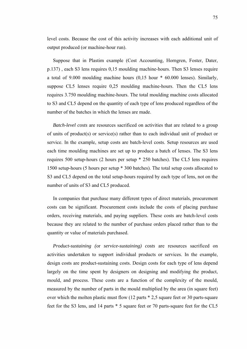
75
level costs. Because the cost of this activity increases with each additional unit of
output produced (or machine-hour run).
Suppose that in Plastim example (Cost Accounting, Horngren, Foster, Dater,
p.137) , each S3 lens requires 0,15 moulding machine-hours. Then S3 lenses require
a total of 9.000 moulding machine hours (0,15 hour * 60.000 lenses). Similarly,
suppose CL5 lenses require 0,25 moulding machine-hours. Then the CL5 lens
requires 3.750 moulding machine-hours. The total moulding machine costs allocated
to S3 and CL5 depend on the quantity of each type of lens produced regardless of the
number of the batches in which the lenses are made.
Batch-level costs are resources sacrificed on activities that are related to a group
of units of product(s) or service(s) rather than to each individual unit of product or
service. In the example, setup costs are batch-level costs. Setup resources are used
each time moulding machines are set up to produce a batch of lenses. The S3 lens
requires 500 setup-hours (2 hours per setup * 250 batches). The CL5 lens requires
1500 setup-hours (5 hours per setup * 300 batches). The total setup costs allocated to
S3 and CL5 depend on the total setup-hours required by each type of lens, not on the
number of units of S3 and CL5 produced.
In companies that purchase many different types of direct materials, procurement
costs can be significant. Procurement costs include the costs of placing purchase
orders, receiving materials, and paying suppliers. These costs are batch-level costs
because they are related to the number of purchase orders placed rather than to the
quantity or value of materials purchased.
Product-sustaining (or service-sustaining) costs are resources sacrificed on
activities undertaken to support individual products or services. In the example,
design costs are product-sustaining costs. Design costs for each type of lens depend
largely on the time spent by designers on designing and modifying the product,
mould, and process. These costs are a function of the complexity of the mould,
measured by the number of parts in the mould multiplied by the area (in square feet)
over which the molten plastic must flow (12 parts * 2,5 square feet or 30 parts-square
feet for the S3 lens, and 14 parts * 5 square feet or 70 parts-square feet for the CL5

76
lens). The total design costs allocated to S3 and CL5 depend on the complexity of the
mould, regardless of the number of units or batches in which the units are produced.
Design costs cannot be linked in any cause-and-effect way to individual units of
products or to individual batches of products.
Facility-sustaining costs are resources sacrificed on activities that cannot be
traced to individual products or services but support the organization as a whole. In
the example, the general administration costs (including rent and building security)
are facility-sustaining costs. It is usually difficult to find good cause-and-effect
relationships between these costs and a cost allocation base. This lack of a cause-
and-effect relationship causes some companies not to allocate these costs to products
and instead to deduct them from operating income.
3.3 A Framework for Mapping Cost Flows
In the valley of the blind, even the one-eyed man is king! Professor Robert Kaplan
of the Harvard Business School used those words at a cost management conference
in Nashville, Tennessee, on May 18, 1994. He was implying that with limited
visibility or manageable cost data problems, many companies can get by. But with a
substantially more powerful costing approach like ABC/ABM, companies can make
much smarter decisions and sharper assessments, and more frequently (Cokins,
1996).
3.3.1 The CAM-I Cross of ABC/ABM
In 1990, the noted author and lecturer Dr. Peter Turney and management
consultant Norm Raffish created a diagram to represent an activity-based cost
management framework to benefit member companies of the not-for-profit
Consortium for Advanced Manufacturers-International (CAM-I). Within CAM-I, the
Cost Management Systems (CMS) program has provided a forum for leading
thinkers in industry, academia, and government to collectively challenge and
improve cost management systems. As shown in Figure 3.10, the diagram commonly
referred to as the CAM-I cross.

77
Figure 3.10 Multiple cost flows
The diagram reveals in a simple fashion that the work activities in the intersection
of the cross are integral to reporting both the costs of processes and the costs of the
work objects. The work objects are the persons or things that benefit from incurring
activity costs. Examples of final cost objects are a component part of an assembled
product or a specific customer. The vertical cost assignment (ABC) direction
explains what things cost and is called the cost object view, whereas the horizontal
process view (ABM) explains why things cost and what causes costs to exist.
The vertical ABC product view is very effective at capturing how the diversity of
things, like different products or various customers, can be detected and their costs as
reassigned by first measuring resources through their consuming activities and then
into the form of final cost objects. In contrast the horizontal ABM process view is
very effective at displaying the cost terms the end-to-end alignment of activities of a
business process. Since a process is defined as a sequence or network of two or more
activities with a common purpose, a process’ costs are additive regardless of an
activity’s defined level of detail. In addition, the ABM process view can provide
nonfinancial, operational information about activities, such as inputs, outputs,
constraints, and enablers. The ABM process view is frequently called the supplier
value chain, and its costs are interpreted using process value analysis (PVA).

78
Figure 3.11 Activities are central to both views (Cokins, 1996)
In an ABC/ABM system, the total resource costs will always reconcile to the total
process costs and the total object costs. It is a closed cost system with dual measures
that pivot around work activities. This is a key point. Traditional cost systems start
with which ledger account balances get charged with an expense. In contrast, ABC
starts with work activities, not people or their wages, as the origin of thinking. This
makes ABC a socio-technical tool, not just a reporting tool.
3.3.2 The Product and Service Line View (ABC)
Although today’s acceptance and practice of activity accounting is being boosted
by the managerial revolution toward process and systems-based thinking, it was
actually ABC that initially fuelled the interest in the early 1980s. Regardless of
activity accounting’s true genesis, it is important to understand origins of ABC
before learning how the data used for product costing also support process and
performance improvement.
The major distinction between traditional cost accounting and ABC is that ABC
uses non-single-unit production volume cost drivers to trace or reassign activity costs
to products or services. In contrast, traditional systems allocate all indirect, variable
overhead costs to final cost objects by assuming the overhead’s consumption varies

79
at exactly the same rate as a single unit of volume, like a labour hour, a machine hour
an assembled unit of output, or a dollar of purchased material. Allocations assume
overhead varies with these factors one-to-one. ABC knows that overhead is more
complex, that it doesn’t vary with output in that way.
With ABC, an activity cost driver stated in terms of a unit of output is used to
compute a cost rate for each activity. Subsequently, the activity cost is traced or
reassigned to a unique cost object on the basis of how many units of output each
activity consumes during a defined period.
In summary, ABC can detect proportionate consumption of resources in an
organization’s interrelated activities; the organization can then reassign the flow of
costs into a diverse mix of final cost objects comprised of products, customers, and
product sales orders.
3.3.3 Expanding the CAM-I ABC/ABM Cross
Providing ABC/ABM data to end-users is like turning up the lights in a dark
room. It’s useful for seeing performance improvement opportunities. ABC/ABM
illuminates the content of work in verb-adjective-noun grammar (e.g, “rework
defective parts) and presents the costs of business processes across traditional
department boundaries. But rearranging the furniture and cleaning house is what
ABC/ABM is really all about. That is, ABC/ABM does more than just provide
greater visibility and new insights; it enables organizations to make changes. Figure
3.12 expands the CAM-I cross to include the decision-making and diagnostic
capabilities that are supported by cost data.

80
xa∑
Figure 3.12 Integrated cost management (Cokins, 1996)
Experienced, successful users of ABC/ABM systems from different companies
regularly communicate with each other by phone or at forums to share their
applications of the data. Few of these companies are using the data as a tool to
control spending. To date, there has been little evidence of after-the-fact spending
and variance-to-standard analysis using ABC/ABM information strictly for control
purposes. There probably never will be such uses. ABC/ABM is best applied as a
forward-looking planning tool, not a historical reporting tool. The most popular uses
of ABC/ABM data fall into three broad, overlapping sets of decision and diagnostic
capabilities:
1. Activity-based costing simply reports what things truly cost without the
grotesque distortions from flawed or unnecessary overhead cost practices.
This new look at old data often brings surprising reversals of what the
traditional and misleading accounting system reported as profitable and
non-profitable product and service offerings. Organizations tend to use
ABC data more for strategic decisions. ABC also computes the cost of a
process output, for example, the total cost to process an invoice. ABC
brings allocation-free, increased accuracy.

81
2. Activity analysis supports the managerial movement toward continuous
improvement and concentrates more on diagnostics and tactical issues. It
gives less attention to what things costs and more attention to what causes
or drives costs (i.e., activities) – that is why things cost. Activity analysis
(ABM) stems from the new visibility of costs that were hidden in the
traditional accounting system. The scoring or grading of activities and
processes for their value-content or near-term incapability is a popular
extended use of baseline ABM data. Employees can reduce costs by
identifying activities that add little or no value. ABM data help prioritize
where to alternatively spend problem-solving time and energy for quicker
payback.
3. Forward planning and predictive modelling is emerging as the most popular
application of the ABC/ABM data. Once an ABC cost consumption model
is completely built, it has been, in one sense, calibrated. It becomes the
simulation cost model for the entire enterprise. The model’s activity cost
driver rates, for example, are reliable for reasonable time periods assuming
a relevant range. These rates can be used in conjunction with forecasted
quantities of drivers in various scenarios, thus enabling the enterprise to
predict future costs. This makes the ABC/ABM data a natural for decisions
involving cost-estimating such as order quotations, make-versus-buy
analysis, and investment justifications. ABC/ABM is truly a resource
consumption modelling tool.
3.3.4 Unveiling the Expanded CAM-I Cross
Prior to tracing activity costs to their final cost objects, an organization can
analyze, evaluate, improve, or reengineer processes without knowing precisely what
a specific product or service costs. The focus is on the process. This partly explains
why cycle-time compression and TQM initiatives are so popular. Their premise is
that by improving on time or quality, costs will eventually take care of themselves,
somehow exiting the organization.

82
Flowing costs simply provides data. The decisions made with the data bring life to ABC/ABM.
ResourcesDirect
material & labour
Flow of costs to cost objects Decision capability
Indirect work activites
Direct activities
Processes
Why?
Cost dataActualEstimatedPredictive
xa∑
To what?orfor whom?
Projects, support
Products and services
Suppliers
Customers/ orders
Mix of objects of work
Trend analysis Performance measuresProcess
Make vs. buy
Supplier certification
Product mix rationalization
Target costing
Concurrent engineering
New product design
Business process
reengineering
Process value analysis,
benchmarking, cost of quality
Pricing, quoting
Cost driver analysis, trade-offs
Profitability analysis
Investment justification and prioritization, activity-based budgeting, life cycle costing
Fact-Based Decision Capabilities
3Forward
Planning/PredictiveModelling
2Activty
Analysis
1Activity-Based
Costing
Figure 3.13 Fact-based decision making (Cokins, 1996)
The importance of assigning costs to processes prior to embarking on continuous
process improvement and total quality management projects cannot be understood.
Although these improvement endeavours may appear worthy, without relevant and
true cost data, an organization cannot adequately predict the cost impact they may
have. Arguably, it may not even easily identify the opportunities for improvement.
Here are some basic characteristics about a business process. They should be:
• The defined with inputs, outputs, constraints, enablers, and identification of
ownership. A customer must exist for the outputs.
• Controlled and monitored to detect process variation outside acceptable limits.
• Effective in doing the right things.
• Efficient in doing those right things well
• Adaptable, with flexibility to respond quickly to unplanned changes.
Managers and employees are always trying to stabilize processes, but unplanned
forces bring imbalances to the business system. Often, reactive expediting and fire
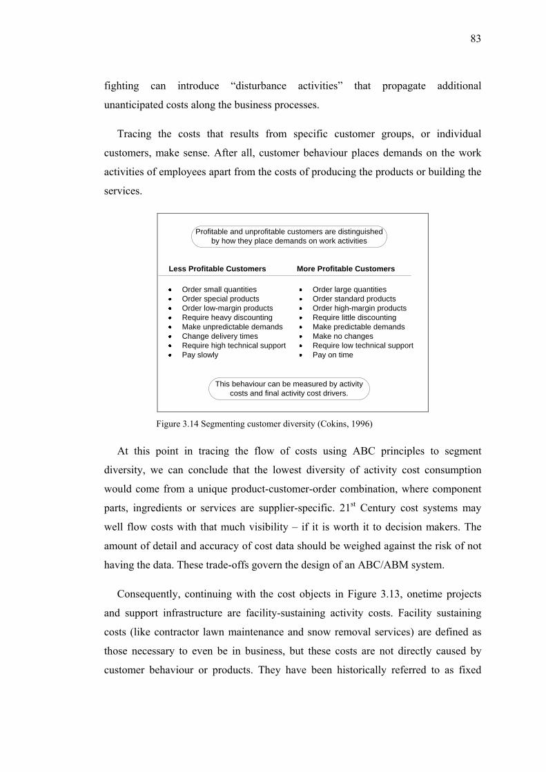
83
fighting can introduce “disturbance activities” that propagate additional
unanticipated costs along the business processes.
Tracing the costs that results from specific customer groups, or individual
customers, make sense. After all, customer behaviour places demands on the work
activities of employees apart from the costs of producing the products or building the
services.
Profitable and unprofitable customers are distinguished by how they place demands on work activities
Order small quantitiesOrder special products Order low-margin products Require heavy discountingMake unpredictable demands Change delivery times Require high technical supportPay slowly
Order large quantitiesOrder standard products Order high-margin products Require little discountingMake predictable demands Make no changesRequire low technical supportPay on time
Less Profitable Customers More Profitable Customers
This behaviour can be measured by activity costs and final activity cost drivers.
Figure 3.14 Segmenting customer diversity (Cokins, 1996)
At this point in tracing the flow of costs using ABC principles to segment
diversity, we can conclude that the lowest diversity of activity cost consumption
would come from a unique product-customer-order combination, where component
parts, ingredients or services are supplier-specific. 21st Century cost systems may
well flow costs with that much visibility – if it is worth it to decision makers. The
amount of detail and accuracy of cost data should be weighed against the risk of not
having the data. These trade-offs govern the design of an ABC/ABM system.
Consequently, continuing with the cost objects in Figure 3.13, onetime projects
and support infrastructure are facility-sustaining activity costs. Facility sustaining
costs (like contractor lawn maintenance and snow removal services) are defined as
those necessary to even be in business, but these costs are not directly caused by
customer behaviour or products. They have been historically referred to as fixed

84
costs. Any attempts to allocate facility-sustaining costs to parts, products, suppliers,
or customers are strictly arbitrary. Since these costs, are outside the direct control of
the process-owners responsible for satisfying product-customer-order combination,
they should be reported separately. The facility-sustaining costs should be isolated
but visible, and termed a surcharge or an enterprise tax.
3.3.5 Industry-wide ABC/ABM: Efficient Consumer Response (ECR)
The retail and food industries are recognizing that their suppliers’ and customers’
behaviours generate a significant amount of their operating costs. These industries
have coined the terms efficient consumer response (ECR) and quick response (QR),
supply-chain language that links the total business process from the dirt and raw
materials to the end consumer.
The key to successfully implementing ECR and QR is recognizing that the
customer is truly very important and conflicts between the manufacturers and
retailers that precede the customer in the supply chain must be resolved. In most
manufacturer-retailer relationships, the two constantly wrestle with each other to gain
the next increment of profit. The wrestling introduces extra costs transparent to the
end-consumer.
ECR and QR programs dramatically deemphasize us-versus-them mentality by
helping all the companies linked in the supply chain to view themselves a single,
unified virtual company. As these industry wide participants realize their
collaboration produces mutual benefits, they learn to share data and technology,
create common standards, and understand each other’s cost economics. This enables
manufacturers, wholesalers, and retailers to maximize profit along the supply chain.
The primary enablers for ECR and QR are:
1. Electronic commerce, including electronic data interchange (EDI)
2. Continuous stock replenishment, which links:
Category management, which monitors point-of-sale data and item
shelf-space allocation data.

85
Flexible, lean, and agile manufacturing and distribution.
3. Activity-based costing and management.
Collaboration among trading partners requires increases in mutual trust, which is
obviously lacking given decades of us-versus-them behaviour. The use of
ABC/ABM data not only replaces intuitions and opinions with facts; it also allows
multiple parties to more quickly agree on how they can change their behaviour to
consequently reduce unnecessary demands for work, thus costs, on each other.
Trading partners must tie themselves together.
3.3.6 Integrating Process Management to Financial Results
Figure 3.15 is an overarching diagram of the relationships between business
process, decisions, and financial results. To the far right are the economic value
added (EVA) financial results. EVA is emerging as the premier measure for
monitoring period-to-period creation or destruction of shareholder wealth. It is
becoming a popular executive compensation tool because it overcomes some of the
flaws of earnings per share (EPS) and return-on-investment (ROI) measures. EVA is
also used for allocating capital investments to the highest-yielding opportunities.
Figure 3.15 Decisions produce results (Cokins, 1996)

86
3.3.7 The Emergence of Lean and Agile Competition
The contemporary forces that are leading to more fierce competition have been
discussed frequently in speeches and articles: global competition declining profit
margins, customer demands, and so on. Figure 3.16 condenses the migration toward
mass customization from an economy initially based on agricultural and natural
resources. We are moving toward an Information Age in which large mass-
production organizations either collide or collaborate with the niche specialists from
the Industrial Age. Alliances of organizations, some for only short terms, are
predicted to abound, creating virtual enterprises.
The implication for agile, lean, and virtual organizations with regard to
ABC/ABM become evident as we move from Industrial Age structures to
Information Age ones:
Industrial Age Organizaitons Information Age Organizations
Nominal overhead costs relative to direct costs.
Sizable overhead support costs of technology dwarfing direct costs.
Focus on growth.
Traditional overhead allocators are poor and misleading cost drivers.
Flexible processes, customized products with information-added services.Focus on value, quality, service, time, and costFocus on being the right size to match customer demand.
Labour or material volume was acceptable proxy for allocating overhead costs.
Mass production with standard products.
Focus on efficiency.
Figure 3.16 The emergence of agility (Cokins, 1996)
87
Traditional accounting, a consequence of 19th-century capitalism, satisfies
stockholders, bankers, and regulators, not business managers. It is backyard-looking
and reports data at too aggregated a level in scope and time for managers to use for
predictive planning. It doesn’t reflect the business process flow very well and is
inadequate for tracing shared service costs into the end products and customer
services that are ultimately sold to generate profit.
It is becoming apparent that 21st-century Information Age organizations will
leverage collaboration, have flat hierarchies of people, rely on concurrent (not
sequential) and parallel from-concept-to-cash processes, and use agile performance
measures, often referred to as a balanced score card. It is inconceivable these
organizations will be able to make trade-off decisions without ABC/ABM. In the
Industrial Age, the customer and financial community were tolerant, lenient and
mostly unknowledgeable of business errors. In the Information Age, the cost of
taking risks without gauging the likely consequences will be large. ABC/ABM
enhances the kinds of critical decision making that managers and employee teams
will be regularly dealing with.
3.4 ABC Is about Flowing Costs
All costing techniques involve reassigning costs by flowing or tracing costs from
general ledger account balances to someplace else. For example, traditional
manufacturing product costing flows an aggregate of overhead cost balances into
products using a single cost allocator or driver, usually labour or machine hours.
When more accurate product costs were eventually needed, accountants began using
multiple cost drivers to reflect the segmentation of diversity and capture
proportionate cost consumption of resources by different products or customers. Now
that organizations are placing greater attention on managing cross-functional
business processes, organizations need to expand from two-stage cost flow
calculations to ones with multiple-stage cost flows and multiple cost drivers. This
better segments the diversity of how activity costs flow into other activities plus
gives visibility to underlying processes (Cokins, 1996).

88
3.4.1 Tracing the Flow of Costs from Resources to Final Cost Objects
In the two stage ABC approach, subaccounts of the general ledger are distributed
to the various activities in the appropriate proportions using, as they are called in
ABC lingo, first stage resource cost drivers. The distributions are based on employee
estimates of what activities consume their time and how much. The costs
accumulated in these activities are then distributed and reassigned directly to final
cost objects using second-stage activity cost drivers, such as the number of orders.
For instance, costs like employee fringe benefits and electrical powers might initially
be distributed to activities using employee head count and machine hours,
respectively, as first-stage resource drivers. Costs accumulated in the various
activities are then further traced and reassigned to products using second-stage
activity cost drivers such as the number and mix of machine setups, sales orders,
purchase orders, machine hours, labour hours and so forth.
Figure 3.17 shows how an early two stage ABC model computes activity cost
driver rates. Those rates become the basis for reassigning the activity costs to each
part, item or service according its unique consumption pattern. That is, the cost
driver unit cost rate is equal to the total activity cost divided by the quantity of
activity outputs.
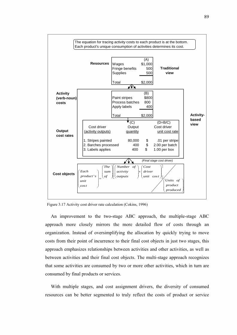
89
(A)Wages $1,000Fringe benefits 500Supplies 500
Total $2,000
(B)Paint stripes $800
Apply labels 400
Total $2,000
(C)Cost driver Output
(activity outputs) quantity
.01 per stripe2.00 per batch1.00 per box
1. Stripes painted 80,000 $2. Barches processed 400 $3. Labels applies 400 $
Process batches 800
(D=B/C) Cost driver
unit cost rate
The equation for tracing activity costs to each product is at the bottom. Each product's unique consumption of activities determines its cost.
ResourcesTraditional
view
Output cost rates
Activity (verb-noun) costs
Activity-based view
' cos
cos
The Number of CostEach sum activity driverproduct s of outputs unit t
Units ofunitproducttproduced
⎡ ⎤⎛ ⎞ ⎛ ⎞ ⎛ ⎞⎢ ⎥⎜ ⎟ ⎜ ⎟ ⎜ ⎟×⎛ ⎞ ⎢ ⎥⎜ ⎟ ⎜ ⎟ ⎜ ⎟⎜ ⎟ ⎜ ⎟ ⎜ ⎟ ⎜ ⎟⎢ ⎥⎝ ⎠ ⎝ ⎠ ⎝ ⎠⎣ ⎦⎜ ⎟ =
⎛ ⎞⎜ ⎟⎜ ⎟⎜ ⎟
⎝ ⎠ ⎜ ⎟⎜ ⎟⎝ ⎠
(Final stage cost driver)
Cost objects
Figure 3.17 Activity cost driver rate calculation (Cokins, 1996)
An improvement to the two-stage ABC approach, the multiple-stage ABC
approach more closely mirrors the more detailed flow of costs through an
organization. Instead of oversimplifying the allocation by quickly trying to move
costs from their point of incurrence to their final cost objects in just two stages, this
approach emphasizes relationships between activities and other activities, as well as
between activities and their final cost objects. The multi-stage approach recognizes
that some activities are consumed by two or more other activities, which in turn are
consumed by final products or services.
With multiple stages, and cost assignment drivers, the diversity of consumed
resources can be better segmented to truly reflect the costs of product or service

90
proliferation and operational complexity. Following this multiple-stage ABC
approach, costs move from initial incurrence to intermediate cost objects in a series
of financial tree-branching arterial decomposition steps, all based on cause-and-
effect relationships using activity cost drivers.
ABC is a little more complex than what we have described up to this point. To segment resource consumption to reflect variety and
diversity, ABC models expand somewhat
Resources
Objects
Activities
Resources
ObjectsSimple ABC
Expanded ABC
Figure 3.18 Multilevel cost flowing
Although the initial assignment of general ledger costs to activities is usually
completed using time effort estimates, the subsequent reassignment of the
progressively accumulating activity costs to other activities is accomplished using
intermediate activity cost drivers. Ultimately, costs are flowed or reassigned to their
final cost objects, such as end-products or customers, using final activity cost drivers.
Multiple-stage ABC decomposition is really a series of reassigning costs along
flow lines called cost assignment paths. The cost data can be captured both on an
incremental and on a cumulative basis on its way toward the total cost of the final
cost objects. The initial assignment translates the general ledger account balances
into activities. Total costs are reassigned.

91
3.4.2 The Evolution of Overhead Cost Systems
In an ideal world, all resource costs could be directly charged or assigned from a
people or machine resource to a specific product or service customer. But in our
practical world, there is so much complexity and technology that most resource costs
are initially incurred in the form of indirect overhead.
The first two generations or approaches represent traditional cost accounting
systems with whole departments’ costs uniformly allocated, usually using arbitrary
and inappropriate factors like square feet or head count. The last three generations
are increasingly activity-based and grow in progressiveness from left to right.
The simple ABC approach uses activity cost drivers that are not tied to units of
volume input/output, such as labour hours, sales dollars, or completed products or
services. This approach subdivides whole departments of people by using action
verb-adjective-noun descriptions of activities. But in the simple approach, the work
described as activities is not related or sequenced end-to-end.
The flexible ABC approach begins adding more stages of cost redistributions to
give more freedom to segment cost diversity. As a result, product, service, or
customer related costs can be computed more accurately. The individual activities
remain insensitive to their sequential relationship in an end-to-end process. This
ABC model does not need to know, nor care, how activities relate to each other
within a business process. It primarily aims to financially decompose activity costs
with little regard to operational uses of data.
The advanced ABC approach incorporates process-based thinking. The activities
are now linked end-to-end as a process chain network or web like artery system. This
advanced approach usually has well over three stages of cost redistributions to
segment diversity, variety, and uniqueness.
Advanced ABC better facilitates process-based management. This is the direction
the cost management revolution is headed. Activity related information is used to
manage the activities performed and understand their causes in order to reduce the

92
costs consumed by those activities. Improved and more accurate product or customer
costing is a natural by-product of process cost model.
3.4.3 Cost Push versus Demand Pull ABC System
ABC software vendors initially chose one of two methods to calculate and
reassign costs: (1) activity-based cost decomposition or (2) customer consumption
demand. Both methods trace and reassign 100 percent of an organization’s costs.
Their differences are in the direction they trace the costs.
The alternative ABC calculation method starts with the cost objects and, working
in the opposite direction, asks which primary activities are consumed and how much.
Customer demand is the driving force. Support or secondary activities are similarly
consumed by the primary activities. The activities are viewed as consuming the
resource costs of payroll and purchase items or services. This method results in ABC
cost flow designs that more physically mirror the business process flow work steps as
compared to the activity cost decomposition method. By declaring standard activity
cost driver rates, this method allows isolating excess capacity costs for each activity.
It is easier to achieve accurate cost object costs through the activity cost
decomposition approach because its cost flow network is unconstrained by
requirements to chronologically link activities to other activities. In contrast, the
process flow approach mirrors the physical reality of how work gets done, which
appeals to those focusing on the costs of the process. However, the process flow
demand pull approach can concurrently trace and keep track of the various diversities
through the network. In the end, the total costs reassigned by each approach must be
equal, and both approaches can be designed such that those totals are also equal for
each final cost object.

93
3.4.4 Elements of Resource Costs
An important step in developing the ABC system’s cost flow is to initially
organize its elements of resource cost into two categories: material costs and activity
costs.
Consider material costs to be all non-payroll costs representing purchases that are
moderately related and conveniently traceable to a specific product or service. Most
of these types of cost, like raw materials, are obvious and have traditionally been
treated as direct costs.
Activity costs are the people and equipment-based conversion costs involved in
performing or supporting the activities that take place within the organization. These
costs would include all labour and fringe benefit costs, as well as other closely
associated “super-fringe benefit” costs, like laptop computers or phone bills,
normally treated as overhead in a traditional cost accounting system. For key
equipment activities, the costs include amortized depreciation. Refer to Figure 3.19.
Figure 3.19 Two categories of resource costs (Cokins, 1996)
Material costs can be traced directly to the products or services whose throughput
measures drive the costs. For instance, the raw materials, purchased components, and

94
some outside contractor services that go into a manufactured product are all driven
by the units of throughput of that particular part. An example would be a hospital’s
purchase costs for each x-ray that requires the same variety and size of film.
Activity costs, on the other hand, are people and machine-related and are traced to
the activities whose drivers make the costs necessary. Indirect material and supplies
as well as other contractor services can be traced to intra-activities where they
eventually get traced to final cost objects. Once accumulated in the activities, the cost
of each activity is traced to each product or service, or to another activity whose
drivers make the activity necessary.
3.4.5 Usefulness of Indented Code Numbering Schemes
Indented code-numbering schemes allow displaying the subtotals of a total.
Subtotals can be repeatedly nested below the total they make up.
Indented coding schemes simplify the following of costs by allowing a downward
decomposition of activity costs and dividing wholes into their pieces. The same
indented coding schemes also allow upward summarization and cost roll-ups to
higher aggregates. Remember that the most detailed data will always be captured at
the lowest level verb-adjective-noun code for an activity, and every cost reported
above it must be a sum total created by formula or equation.
One’s initial impression of subdividing activities with indented code-numbering is
in the direction of levelness – activities are broken into tasks. But there is also a
direction of diversity caused by the cost object driver. The same activity can be
divided by what or whom it serves to improve granularity. The factors influencing
the ABC model design will always swing between process view and product view.
Business processes were previously defined as a sequence or network of activities,
regardless of the activities’ level of detail. By decomposing functional areas into
large numbers of activities for the purpose of segmenting diversity, the activities can
be recombined to understand costs across the core business processes. For instance, a
business can determine all of the costs involved in the process used to procure

95
needed raw materials, purchased components, indirect materials, and outside
processing services. First, the functional areas such as purchasing, material handling,
shipping, receiving, inspection, accounts payable, and quality control are
decomposed into verb-adjective-noun activities that describe employee efforts in the
procurement process. Then, only those activities from each functional area that apply
can be recombined into the process to arrive at the desired cost information.
3.4.6 Scoring Activities to Facilitate Managerial Analysis and Actions
Organizations interested in performance improvement can use grading methods to
evaluate the activities that contribute to the output of goods or services according to
whether or not the activities are necessary, support critical strategic success factors,
or the performed efficiently. Various coding methods are used for this scoring of
activities; these range from the very simple value-added/non-value-added approach
to differentiating methods using very complex criteria. The idea is to eliminate non-
value-adding activities and optimize value-adding activities, thus enabling employees
to focus on the worth of work. Focus and visibility are enhanced because people can
more easily see where costs are big or small and what costs can be impacted or
managed in the near term.
The most popular differentiating categories are often called activity metrics or
attributes and they are attached to the activity costs:
Impactability or urgency.
Value-added content.
Effectiveness in performing the activity.
Importance in supporting management’s strategic plans.
Quality content.
Cost influencing content.
In addition to categories, there are multiple views from which to grade activities:
From a customer’s or process owner’s view.
From the product or service’s view.

96
From enterprise strategy’s view.
From an efficiency view.
Employee teams usually customize their own approach by differentiating
categories from multiple views and defining the scoring scale for multiple views and
defining the scoring scale for each specific category using complex criteria. The
underlying principle is that activities can be scored or graded at the lowest activity
level, like a gene in a chromosome, which then allows the scored cost to uniquely
accumulate into any cost roll-up or cost recombination involving two or more
activities. Insights are gained as the marked activity dollars are combined, and then
analysis can show both where and how intense problems or opportunities might be.
The employees who score or grade can be a different team than the employees or
functional representatives who defined the activities and estimated costs.
• Degree of impactability or urgency. Each lowest-level activity can be
graded for its near-term and long-term impactability as high, medium, low,
or none. Alternatively, a percent of impactability can be estimated for each
activity to test and quantify the aggregate cost savings opportunity that
currently is based on a gut feeling or a non-quantitative, non-dollarized
judging scheme. Employees usually score an activity’s impactability high if
they believe it is non-value-adding. As an option, activities can also be
graded by the necessity to change their consumption level in order to align
activities with strategic goals or to remove waste.
• Value-added content. This scoring scheme has evolved over time. This
evolution has moved from a focus on the dichotomy of either value-added
or non-value-added, to the degree of value-added, to value-creating from a
customer’s view value-enabling product from a product’s or process’ view,
non-value adding from all three of those views, and the degree of value
added.
• Effectiveness level. This scoring scheme assesses how well the performance
meets the activity or process customer’s expectations.

97
• Importance level. This scoring scheme relates each activity to how well it
supports management’s strategic goals. A test question for each activity is,
“If we stopped this completely, what would be consequences?”
• Quality content. This scoring scheme, shown in Table 3.1, classifies each
activity and supports the popular TQM categories as follows; cost of
conformance (prevention activities and appraisal and test activities), and
cost of non-conformance (internal failure activities and external failure
activities).
• Cost influencing content. This scoring scheme attaches and associates a
specific upstream activity with a specific downstream activity that was
caused upstream. There is an effect-based relationship between activities.
Table 3.1 Cost of quality using activities
Training Advanced quality planning Perform SPC Fool proofing
Incoming inspection Editors' review Line inspection Approvals Finished goods inspection
Process scrap Rework Unplanned downtime
Handle complaints Warrant changes Process returns Expedited late order Lawsuits.
Activities designed to prevent errors and mistakes during make and delivery
Activities to review, audit, evaluate, or measure to assure conformance
Activities correcting errors prior to customer receipt.
Activities correcting errors after customer receipt
Conformance NonconformanceI
PreventionII
AppraisalIII
Internal failureIV
External failure
Companies can assign activity attributes to cost of quality (COQ) categories.
Take actions to shift costs to lower overall COQ
tivity oupamples
efinitionsoup
xamples
Consequently, the scoring of activities brings colours and shadings to the
ABC/ABM model; without such scoring, all dollars are devoid of any nonmonetary
value. By differentiating dollar cost with scoring and grading schemes, the
managerial analysis is greatly improved and attention and focus of employees can be
better directed.

98
3.5 ABC versus Theory of Constraints versus Throughput Accounting
In the early 1980s, a physicist specializing in fluid dynamics named Eliyahu M.
Goldratt captivated operations managers’ attention with his Theory of Constraints
(TOC), an approach to material flow control based on bottleneck properties. He
mesmerized people not only with the simplicity of the theory’s approach but also by
describing major flaws in traditional full-absorption accounting (Cokins, 1996).
Goldratt would described how the accountants’ cost allocation practice of
applying overhead costs to products on the basis of labour hours or machine hours is
also used to measure a work centre’s utilization and efficiency performance.
Measuring the productivity of a work centre without regard to the total system
inadvertently motivates behaviour that, while individually appearing good,
collectively is contrary to just-in-time managerial thinking and adversely affects the
total organization’s efforts.
One of Goldratt’s mantras is “The sum of the local optimums will never exceed
the global optimum.” So in conjunction with explaining what is bad about traditional
cost accounting, Goldratt also provided a vision of what a better replacement cost
system would look like. Having both a criticism and a solution is a basic formula for
overcoming organizational resistance to change. His replacement costing approach is
simple and very appealing to logic:
You start with basic assumption that the goal of any profit-making business is
to make money.
The replacement cost accounting then falls neatly into place by focusing on
the three possible dimensions of money:
I. Throughout (T) – the rate at which the system (i.e., the business)
generates money through sales.
II. Inventory (I) – all the money the system invests in purchasing things it
intends to sell (i.e. direct and associated indirect materials).

99
III. Operating expense (OE) – all the money the system spends in
converting inventory into throughput (e.g. wages, fringe benefits,
depreciation, capital charges, support costs etc.).
Throughput costs effectively become the total sales less purchased direct material.
Inventory costs are not comparable to the financial accountant’s goal of constantly
attaching on-the-fly expenses for point-in-time valuation of work-in-process or
finished goods inventories. Theory of Constraint (TOC) cost accounting obviously
adapts a different view that disregards interim valuation of inventory.
This new of costs brings greater emphasis to material flow velocity and has
spawned the name throughput accounting. It recognizes that capacity constraints are
gating factors to making profit and that any time lost at a bottleneck is forever lost to
the total business and results in lost profit.
TOC advocates assume that much or all of the overhead cost allocations can be
loaded at the bottlenecked work centre. This escalates the cost of any part, product,
or service that uses that work centre, which conversely reduces loaded costs to
similar items going through non-bottlenecked work centres. The resulting
calculations yield dramatically different product costs and clearly penalize items
‘renting time’ at the bottleneck. The new cost measures are used to understand
directionally where incremental product profit may come from and to aid future
planning for capital or resource spending.
Here is one of the rubs. TOC advocates criticize ABC data because it can produce
different cost numbers than theirs. Since throughput accounting supports JIT thinking
and all of the TQM-related philosophies that go with JIT, to TOC advocates ABC
data appear both wrong and bad.
In practice, most operating environments are well balanced with regard to
production rates and available capacities; and managers are getting increasingly
better at flexibly moving people and reprioritizing schedules. Most companies are
moving toward scheduling and dispatching near-term planning systems that include
finite forward capacity logic with much broader views and more frequent schedule
refreshing than in the past. These things are what industrial and process engineers are

100
paid to do. The net effect is that operations are fairly well balanced; any significant
imbalances, which create the bottlenecks, usually come from the demand schedule of
different orders with different due dates. The implication is that the bottleneck
wanders.
ABC data is not volatile. It does not concentrate on the direct costs, which vary
with a high correlation with the output of primary parts, products, outputs, and
services. What ABC does do is concentrate on the costs of all of the other indirect
work activities? ABC acts as a proxy for a direct costing system by linking the
activity costs that support the end-products and services, which appear to many
people as fixed costs. ABC accomplishes this by flowing costs through an arterial
assignment network of cause-and-effect drivers. Therefore, ABC more accurately
captures product costs, which will vary only to degree that the quantities of their cost
drivers vary – and the majority of those costs have little or nothing to do with the
bottleneck or where the bottleneck is located at any moment in time.
TOC advocates find great appeal in accelerating the pipeline’s velocity. By
putting the measurement spotlight on the pipeline, the organization will directionally
know where to spend its incremental dollars. In addition, throughput accounting
removes accountability from all the support costs, which usually include the costs of
the TOC advocates themselves.
Figure 3.20 ABC versus Theory of Constraints (TOC)

101
ABC produces distortion-free visibility to costs, cost behaviour, and cost
accumulation. It provides a foundation from which better decisions can be made,
such as for marginal costing or incremental volume cost justifications. The ABC
foundation is a solid web of cause-and-effect relationships. ABC costs do not gyrate;
they rise and fall to the waves of customer order demand and to quantity changes of
the activity cost drivers. In the end, ABC is simply a mirror in which the organization
can examine its cost economics, particularly its increasingly swelling indirect costs.
The time horizon is actually what seems to divide TOC and ABC advocates. For
instance the TOC camp would claim that the cost of a shortage from missing 50-cent
bolt is worth 100 dollars of premium airfreight, not 50 cents, if its shortage will delay
shipment of a $100,000 order. The cost depends on other circumstances. Few
resource costs in an enterprise are affected by a bottleneck or near-deadline delivery
date. ABC reports actual costs of resource consumption, assuming normal operating
conditions that reflect expediting and reacting behaviour. In contrast, TOC overstates
costs and points to problems that may in fact only be temporary.
3.6 ABC and Unused Capacity Management
In defence of ABC, there is a movement to report the costs to a relevant level of
detail. With more relevant data, it is hoped that the organization will behave
directionally toward the aspiration that Goldratt pronounced: to make money. There
will forever be natural tension between sales and production. ABC data can be
reformatted to remove much of that conflict and introduce a neutral target for both
sales and operations to attack for their mutual benefit. The neutral target for both
groups to focus on is costly unused capacity (Cokins, 1996).
Sales can remove unused capacity by filling it with orders. Operations can remove
unused capacity by streamlining, by removing capacity-consuming yield losses, and
by better scheduling the product or service flow.
This ABC movement starts with the premise that true total capacity should be
measured 24 hours a day, seven days a week, for an entire year. This is technically

102
referred to as theoretical capacity. Within this truly total capacity; one can begin to
measure theoretical capacity’s elements as either containing:
I. Idle capacity – no use for reason of policy, union rules, legal regulations,
holidays, or simply insufficient sales demand.
II. Non-productive capacity – time where resources are either being held for an
expected workload; being used to produce what will subsequently be
discovered as scrap loss or rework; being repaired, serviced, maintained, or
trained; or being set up or changed over to produce the next scheduled
product or service.
III. Productivity capacity – times used to actually work on what the customer is
buying or to practice on or break in new products or new processes.
When capacity is segmented this way – at a fairly granular level, such as by each
producing work centre – both sales and operations personnel can focus on a mutually
enemy: non-productive capacity. Operations people can focus on removing it with
faster setups and higher equipment uptime, resulting in an increase in idle capacity,
which in turn provides an opportunity to fill more sales orders. Salespeople can
remove non-productive capacity by adding more sales orders, which also increases
productive capacity.
In attempting to understand unused capacity, ABC advocates have determined
that managers can segment total theoretical capacity into the three classes above and
measure ABC cost data at individual work centres to that same level of granularity.
And it can even differentiate sunk costs from controllable expenses to the same level
detail.
The next chapter expands on the softer, human issues of overcoming ABC/ABM
implementation obstacles and getting people on board and excited about ABC/ABM.

103
3.7 Implementation
3.7.1 The Difference between implementation and installation
ABC/ABM project managers tend to be those pioneers mentioned earlier who
constantly want to dispense with the theory and fluff. They just want to how-to
instruction manual. It is best to think of ABC/ABM implementation as preparing for
the project that brings about change and ABC/ABM installation. Attempts at ABC
installation without first having success with the implementation is a receipt for
failure. Implementation of ABC/ABM is more craft than science, and those readers
desirous of rule-based designs, algorithms for computations, and linear regressions to
optimize their ABC/ABM models had better step aside until about 1999 while an
interviewing generation of more practical managers apply common sense and use the
insights provided by the new data to make better decisions.
3.7.2 Implementation Roadmap
The roadmap should be understood for the same reason that manufacturers plea
for consumers to read their instruction guide before assembling a kit – there are
things to know before getting to far along into the assembly. Figure 3.21 shows a
highly simplified ABC/ABM implementation roadmap.

104
Figure 3.21 ABC/ABM implementation road map (Cokins, 1996)
3.7.2.1 Implementation Steps (Cokins, 1996)
Step 1. Determine why you are doing ABC/ABM. What is your target? What do
you want to change? Who will be the end-users of the data? Meet with key end users
to validate their dissatisfaction with the current accounting practices and ensure they
know how ABC/ABM will make it better. Then as you progress, have a
communications plan to keep them involved.
Step 2. Throw away the organization chart. Diagram the business processes at a
reasonable level of detail using popular flow chart and process mapping practices
and techniques. Do not make it too summarized or too detailed. Make sure that all
process has inputs, outputs, and customers at the end.
Step 3. Construct and compute an ABM “strawhorse” model. Build an activity
dictionary and collect very high level material and activity resource cost information
based on estimates from a few good employees (or from reasonable alternative data
collection techniques). Using only a single-state cost flow, trace those resource costs
into activities and group them by business processes. The ABM strawhorse model is

105
now complete. It is that simple. Graph the data for visualization to enhance end-user
interpretation, analysis and effect.
If appropriate, further trace activity costs combined as common groups (activity
centres) into high-level final cost objects to better quantify ABC products, customers
and profit margins. Use only a few second stage final activity cost drivers to keep the
straw horse simple.
Step 4. Look for the problems and opportunities. Using a cross-function team,
analyze the ABM value-chain costs that have now been aligned along business
processes. Interpret and discuss findings. Conclude where to focus and consider what
opportunities for improvement exist. Validate previously proposed improvement
opportunities that are funded and already in progress.
Step 5. Prioritize the opportunities for improvement.
Step 6. Using popular diagnostic and analytical methods (root-cause analysis),
explain the causes for problems in the opportunity areas. Gain insights for alternative
solutions.
Step 7. Convert the opportunities into actionable management by selecting
specific improvement projects and initiatives that provide solutions. ABC/ABM has
been called an initiative accelerator.
Step 8. Using the ABC/ABM data, test the potential financial impact of each
project or initiative by quantifying the cost saving, cost avoidance, or revenue
enhancement possibilities. Apply the planned changes to work flow and work
content in the model and the project the new cost behaviour.
Step 9. Make changes. Proceed with altering product and service designs,
changing people’s attitudes, creating shared visions, restructuring work, reorganizing
jobs, removing barriers, or altering the behaviour of suppliers or customers. Make the
processes mistake-proof.

106
Step 10. Are you at point B yet? If not, go back to one of the previous steps and
refine. This is a continuous process, but the ABC/ABM system is a one-time
construction, but always flexible in its design.
Those 10 steps are for the ABC/ABM implementation, not the installation. Steps
2 and 3 are clearly the important ones for building the ABC/ABM system. An entire
ABC/ABM installation roadmap exists in side step3. Starting in installation,
expanding steps 2 and 3 will be the main focus of implementation.
3.7.2.1.1 Measuring Success (Cokins, 1996); Question 1. If the ABC/ABM pilot
is being successful, how would we know it?
Answers:
• The business starts being managed differently.
• The pilot progresses to a next phase.
• End-user interest and requests for feedback increase.
• The new data starts being used and acted on.
• An ABC language emerges among employees.
Question 2. What would be measurable indicators of a pilot’s success?
Answers:
• Cycle times are reduced and quality is increased.
• Performance measurements are reformed with a greater emphasis along
business processes.
• Other continuous improvement programs request or use the ABC/ABM
data.
• Additional improvement projects are simulated.
• A second ABC/ABM pilot is endorsed.
• The number of ABC literate end-users expands.
• The number of decisions applications using ABC data expands.
• A survey of nonfinancial end-users indicates satisfaction with the system.

107
• Additional executive-level sponsors appear.
• Requests for ABC/ABM training increase.
• ABC model updates are frequently requested.
• Products become more profitable.
3.7.3 Up-Front Design Decisions and Caveats
It has said that a successful ABC/ABM system implementation is 5 percent
software with its interfaces and 95 percent a combination of model design and
behavioural change management. Achieving success involves following classic
principles recommended for managing project:
• Define project objectives, which will have measurable indicators as the
milestones are being achieved.
• Recognize the end-users of ABC/ABM data as internal customers and earn
the right to advance with them by continuously giving them something they
value, such as better data or new insights.
• Allow the ABC/ABM system’s scope, size, and level of detail, granularity,
and accuracy to continuously unfold by working backyard from a mutually
agreed-on deliverable that will help end-users solve one of their most
distributing business problems. This advice may appear counter to the TQM
“do it right the first time” philosophy, but rapid prototyping as a learning
device for adults is just a better, more expedient and more practical
approach. ABC/ABM system implementations usually stumble when they
are over engineered and are without a predefined purpose.
Start with a no computerized, grease pencil drawing of your organization’s
ABC/ABM multistage cost flow model before constructing your spreadsheet straw-
horse. The myriad of up-front ABC/ABM installation-related questions about the
number of cost drivers, the number of activities, the choice of cost drivers, the
frequency of model updates, and so on are ultimately best answered by first gaining
experience and then constantly satisfying the internal customer’s needs and wants.

108
A decision must be made as to whether the first ABC/ABM model is intended as a
diagnostic one-time study, a baseline for a repeatable model, or a fully integrated and
automated permanent production system. These three choices are depicted along a
continuum in Figure 3.22.
Figure 3.22 ABC/ABM implementation continuum (Cokins, 1996)
3.7.4 Defining Objectives for Success – Yardstick Measures
ABC/ABM projects can fall short of their full potential. To succeed you must do
more than just (1) understand why ABC/ABM projects don’t totally satisfy objective,
(2) learn from those lessons, and (3) take corrective actions to not repeat others’
implementation errors. Although those are noble goals, it is worth proactively
establishing in advance your own yardstick measures for success of your own
ABC/ABM project.
Common barriers to successful ABC/ABM implementation relate to
accountability in two very different ways. One way previously discussed involves the
initial resistance of internal end-users caused by anxieties that their performance may
be financially measured with techniques other than the traditional measures they’ve

109
artfully mastered over the years. But the second problem involves monitoring the
ABC/ABM implementation project itself. How is the ABC/ABM project’s success to
be measured?
Figure 3.23 Measuring success (Cokins, 1996)
3.7.5 Popular Applications of ABC/ABM data
Since ABC/ABM data are basically used as means to an end, it is important
identify the “end”. Agree on a decision capability for the new data that end users
have really wanted and that will give them positive results when they finally use it.
People will resist reforms to measures even if they know that the one’s they’re
using are bad because they also know how to get around them for personal purposes.
ABC/ABM proponents strongly believe that the use of activity based costing data
and their associated practice is an eventuality.
Table 3.2 Popular applications (Cokins, 1996)

110
Operational ApplicationsHow to condust business? Where to look for opportunities?
Strategic Applications
Performance measurements,Target costingLife-cycle costing
Order quotations (pricing)Product profitability analysis Customer profitability analysis Capital expenditure justifications
Business process/activity value analysisCost-of-quality analysisCost driver analysis (Unit costs of)Make-or-buy analysisBusiness process reengineeringBenchmarkingActivity-based budgetingUnused capacity analysis
3.7.6 Critical Success Factors for ABC/ABM Implementations
The key to successful implementation and sustained use of the ABC data is to
balance the four areas explained in the following:
1. ABC model design and architecture; constructing an ABC/ABM model
combines art, craft, and science.
2. Implementation and integration; It is important to select promising pilot sites
and to involve individuals with information –technology skills.
3. Getting buy-in; Get the support of an executive sponsor and create widespread
interest in and ownership of the data and its uses.
4. Application of the data; be sure there are end-users with strong needs for the
ABC/ABM data.
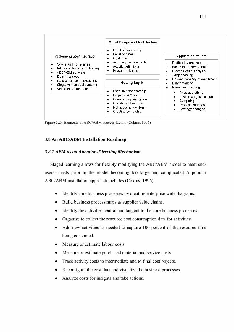
111
Figure 3.24 Elements of ABC/ABM success factors (Cokins, 1996)
3.8 An ABC/ABM Installation Roadmap
3.8.1 ABM as an Attention-Directing Mechanism
Staged learning allows for flexibly modifying the ABC/ABM model to meet end-
users’ needs prior to the model becoming too large and complicated A popular
ABC/ABM installation approach includes (Cokins, 1996):
• Identify core business processes by creating enterprise wide diagrams.
• Build business process maps as supplier value chains.
• Identify the activities central and tangent to the core business processes
• Organize to collect the resource cost consumption data for activities.
• Add new activities as needed to capture 100 percent of the resource time
being consumed.
• Measure or estimate labour costs.
• Measure or estimate purchased material and service costs
• Trace activity costs to intermediate and to final cost objects.
• Reconfigure the cost data and visualize the business processes.
• Analyze costs for insights and take actions.

112
Traditional cost accounting reports expenditures to managers by department or
cost centre. This simply gives managers and employees a stovepipe view of
themselves and actually blocks them from seeing how their enterprise behaves
horizontally by processes and as a tool business system. In effect, traditional, general
ledger cost accounting systems act like thick cloud covers.
What managers initially need is a quick glimpse of what’s below those clouds.
Traditional accounting systems provide little visibility to business processes, and
managers need to understand costs of these processes. These dismal conditions
justify why ABM supply value chain cost data need only be collected and initially
reported using a fast, high altitude flyover technique- dip under those clouds and
snap a few pictures of the enterprises cost use and then interpret what is seen. This
high-altitude flyover in effect becomes the strawhorse mock-up for the eventual
ABC/ABM cost system.
ABM as a Focusing Tool, Supplier value-chain analysis (ABM) at a high-altitude
flyover stimulates managers and employees.
ABC/ABM Begins with Enterprise-wide Diagrams; the starting point of the
installation roadmap is to identify business processes. A popular approach for
identifying them is to use visual diagrams. This is a top-down approach.
3.8.2 ABM as a Focusing Tool
Supplier value-chain analysis (ABM) at a high-altitude flyover stimulates
managers and employees. Finding the answers to the above questions ignites them to
build strong business cases to take actions. In this way, ABM achieves its purpose as
an attention-directing mechanism.
Building compelling business cases, however, may require more specifics and
particulars than provided by the high-altitude flyover snapshots. A better, closer view
gained from a 50,000-foot ABM flyby can help managers focus on the core business
processes. At a granular level, with more code-intended activity levels, the process’

113
cost consumption characteristics will provide greater resolution, become more
visible, and be even better understood by end-users.
By collecting lower level, decomposed activity cost data, more hidden costs,
likely to be favourably affected by a future process change, can be identified and
quantified. The sum of the hidden costs of the core business processes, when scored
and combined with the more obvious non-value and low-value-adding activity costs,
may well tip the scales in a decision of whether or not to proceed with an
improvement initiative or investment.
The ABM value-chain activity analysis can be further magnified with a more
detailed and illuminating 10,000-foot flyby. This data collection and reporting
exercise can also be quick and economical, accomplished in days, not months.
3.8.3 Linking ABM to Relationship Maps Using Process Mapping
Process mapping is synonymous with value-chain analysis. It helps to document
the results of the relationship map and organize information to ensure its complete,
understandable, and readily analyzable ABM configures the organization and assigns
costs to business processes something that traditional accounting cannot achieve.
Until the next generation of managers, relationship diagrams and business process
maps should probably be kept at a summary level. They will need to be graphically
modelled and visualized at an intermediate-to-high level. Fortunately, this is the
same level at which ABM costs should be collected, measured and reported.
Therefore, the cost data can be aligned with processes and maintained in sync with
the messages that are signalled to managers from relationship map.
3.8.4 Identifying Activities within Business Processes
Regardless of an organization’s size or number of employees, a virtually limitless
number of activities can be selected. How do you control the size and number of
activities? The criteria for identification activities should include materiality as well

114
as the objectives of the ABC/ABM data discussed in step 1 of the implementation
road map.
You can maintain materiality by using common sense. Don’t chase details.
Strategic objectives of ABC/ABM can require identifying and defining more
summarized levels of activities than if the objectives are tactical and simply for
operational improvement.
3.8.5 Organizing to Collect Resource Cost Data by Activities
The ABC/ABM system must initially assign resource costs to activities. Resource
costs are continuously captured via transactions in general ledger journal account
balances (payroll, accounts payable, material stores issues, journal entries etc.). The
assignment of these costs to activities can be done.
• By direct charging, using existing measurements (e.g., charging repairs via
a work order, metering fuel consumption, charging supply issues).
• By estimation (by surveying techniques)
• With arbitrary allocations; but these should clearly be resisted because they
don’t aid in better understanding or modelling the economics of the
business.
Direct charging with measured data consumed by its cost object is common sense.
However, dealing with indirect charges requires identifying activities and estimating
the labour and material consumption within each. It is easiest to collect data on
labour and service-time costs before estimating external purchased materials and
contractor service costs. The reason is that concentrating first on what people do
defines a basis on which purchased materials and contractor services can
subsequently be assigned.
Estimating can be controversial because it implies there will be some degree of
error. With ABC, however, knowledgeable estimates from informed individuals are
much more preferable than precise calculations of irrelevant allocations.

115
The first of the three estimating options relies on business process supply chains
as the source for defining activities. Using a predefined process map, which arranges
the organization into a network of labour-performing work, simplifies defining
activities. At the lowest step of each business process, simply describe a few verb-
adjective-noun activities. Repeat this for every step of every business process, and
you’ll eventually construct the activity dictionary.
The second estimating option is useful when there are incomplete or no
documented business process flow charts. This option creates the whole (i.e.,
processes) from the sum of the parts (i.e., the work activities). Each stovepipe,
functional department is surveyed for the employees’ activities in isolation of the
other departments. When all departments have been surveyed, the activity-based
model for the total enterprise is then created by assembling the parts into a whole.
The business processes are rationalized from examining the verb-adjective-noun
activities, and then these activities are sequenced along the business processes.
Table 3.3A shows a time-effort input form that has been completed by a
functional representative. The estimates have been rounded to 5 percent increments.
Table 3.3B shows the cost activities, with average salary and fringe rates used for
each natural work group; the total costs appear in the last column.
Both of the above options are designed to produce rapid, non-invasive results with
a minimum adverse impact on data accuracy and credibility. Both techniques are top-
down and rely on a few good employees as representative estimators. That is, the
ratio of employees to estimators is high. ABC/ABM implementation teams
frequently rotate back and forth between these two options as empty holes of work-
content get defined and filled in. These two estimating options check and balance
one another because they both are describing the same thing: the work people do.
The top-down approach to achieve quick availability and visibility of activity-
based cost data is more effective when the number of functional representative
estimators (i.e., the few good employees) is limited, they reasonably understand their
business, and a financial accounting team member is knowledgeable about general
ledger accounts and balances.

116
Table 3.3A Time-effort input sheet
Date:
Set-up equipment 90%Chase material 25% 10%Inspect finished cards 50%Inspect incoming material 50%Maintain facility 30%Manage program changes 75%Move material 50% 25% 10%Plan printing schedule 25% 75%Store excess material 25%Do unscheduled maintenance 40%Run 1972 standard printer 25% 60%Run 1995 personalized printer 5% 30%Total 100% 100% 100% 100% 100% 100% 100%
1 @ $45K Scheduler
2 @ $ 50K Set-up
Engineers3 @ $ 50K Printers
3 @ $20K Material Handlers
2 @ $20K Inspectors
2 @ $35K Maintenace
2 @ $25K Computer
Programmers
Page_ of _Employee Names /#/Groups & Expenses
Employee and Expense Activity Effort Worksheet (%)
Prepared by Project Manager
Activity
Avg. Wage & No. Emplyoees
Table 3.3B Cost activities
Date:
Set-up equipment $90,000 $90,000Chase material $15,000 $15,000 $30,000Inspect finished cards $20,000 $20,000Inspect incoming material $20,000 $20,000Maintain facility $21,000 $21,000Manage program changes $37,500 $37,500Move material $30,000 $11,250 $10,000 $51,250Plan printing schedule $12,500 $33,750 $46,250Store excess material $15,000 $15,000Do unscheduled maintenance $28,000 $28,000Run 1972 standard printer $17,500 $90,000 $107,500Run 1995 personalized printer $3,500 $45,000 $48,500Total $60,000 $40,000 $70,000 $50,000 $45,000 $100,000 $150,000 $515,500
Employee and Expense Activity Effort Worksheet ($)
Page_ of _Prepared by Project Manager
1 Scheduler
2 Set-up
Engineers3
Printers
Employee Names /#/Groups & Expenses
Total
3 Material Handlers
2 Inspectors
2 Maintenace
2 Computer Programmers
ActivityAvg. Wage & No. Emplyoees
* $135,000 direct labour cost
The third estimating option is a bottom-up, small group technique that relies on
storyboarding which employs cut-and-paste bits of information and flip charts and
involves inverse participation of work groups. It relies on numerous group meetings
of side-by-side employees in which they define what they do and how they do it.
This technique supports total quality management (TQM) improvement philosophies.
Each team member of every work team formally defines work from his or her
117
viewpoint. The employees’ time is then apportioned to their known activities, and the
costs are assembled in a manner similar to that used in the second option.
In practice, companies with successful ABC/ABM systems have used elements
from all three of these data collection options. The advantage of the first two options
is the data can be rapidly collected with relatively high accuracy, consistent
definitions, and initial non-invasive impact on employees. The advantage of the
story-boarding option is there is greater employee involvement, which helps change
personal attitudes, may speed achievement of consensus and minimizes resistance to
change. Regardless of which technique you use, be sensitive to the individuals who
are being honest about the organizations activities.
3.8.6 Measuring Labour Conversion Costs by Percent
The high-altitude flyover and low-altitude flyby data collection approaches
provide increased, scalable information and without distortion. This data can then be
used to measure labour conversion costs. Employees’ average salary and fringe
benefit dollars are multiplied by estimated percentage of the total work that the
employees’ activities account for. Average salaries can be identified at the same
department levels as used during the annual budget exercise.
In practice, gaining estimating accuracy through scaling is accomplished by
merely expanding the size of the activity-by-employee-group matrix or using more
work representative estimators. The followings are ways to get more accuracy:
• The number of natural work groups that are estimated for can be further
subdivided, but the total number of employees will always remain the same.
Natural work groups are two or more employees, not necessarily from the
same department, who perform common activities with related outputs, like
purchasing agents and receiving dock workers. Note that despite subdividing,
the ratio of total employees to estimators remains unchanged.

118
• The verb-adjective-noun activity convention remains unaffected, but the
lowest-level activity column can be expanded by adding an intended column
to the activity dictionary, thus providing another level in detail.
• The number of functional representative estimators can be doubled or tripled
to achieve a more accurate estimate of the incrementally lower level of costs
from the further subdivided natural work groups of employees. This lowers
the ratio of employees to estimators. More estimators assure a greater
familiarity with how work time is apportioned by the employees within
natural work groups.
3.8.7 Measuring Labour Conversion Costs by Cycle-Time Outputs
The cycle-time approach requires a start-to-end process flow chart. An average
cycle time is estimated for each activity, or group of activities. For example, assume
that travel reservationists handle completed ticket reservations and customer
inquiries about schedule times, departures, arrivals, or ticket prices. Also assume the
following (Cokins, 1996):
Average time per completed reservation = 7.50 minutes/output
Number of completed reservations per month = 10,000
Average time per inquiry = 4.00 minutes/output
Number of inquiries per month = 19,650
Number of travel reservationists = 20
Average monthly salary and fringe /employee = $3,000
Average employee hours worked/week = 40.0 hours
Average break time per worker/week = 8.0 hours
A cost per completed reservation and per inquiry can be computed as follows:
$3,000 * 20 =$60,000 payroll per month
40 hours/week – 8 hours week break time = 32 hours * 4 weeks/month =128
hours/month
128 * 20 employees = 2560 person-hours/month

119
Cost factor = $60,000 (load)/2560 (rate)
= $23.4375 /hour or
= $.390625 /minute
Cost per completed reservation @ 7.5 minutes = $2.929688
Cost per inquiry @ 4.0 minutes = $1.5625
One of the complications with the cycle time output approach is reconciling the
total costs. By continuing the cost math:
10,000 reservations @ $2.929688 each = $29,296.87
19,650 inquires @ $1.5625 each = $30,703.13
Total = $60,000.00
In this example, the total monthly costs of the reservations and inquiries fall short
of the $60,000 payroll. In addition perhaps the reservations performed a third
untracked activity like cancelling tickets. A complication with the cycle-time output
measure approach involves:
• Cost and time of the processor (the reservationist).
• The cycle time of the process/activity (reservation, inquiries).
• The quantity of the processes (reservations, inquiries).
The cost-load rates, average processing cycle-time rates, and total cost are usually
determined during measurement periods that differ from the period for which costs
are being accounted.
Correcting this situation is not a major issue. If a complete reconciliation with
period expenditures is the goal, the cost rates can be modified upward or downward
to force the complete reconciliation.
3.8.8 Estimating Purchased Material and Service Costs
The attention thus far for data collection has been strictly on the employee-related
time-effort expenditures (salary, fringe benefits etc.) How do no payroll-related and
purchased material expenditures from third parties get assigned from the general

120
ledger into activities? It is best to restrict these assigned costs to those activities
already defined for what people and machines do. That is, do not create new
activities.
A practical estimating approach involves first isolating a Pareto ranking of
roughly 90 percent of non-wage general ledger account balances for expenses (e.g.
supplies, travel, etc.). Then assign the cost of the larger dollar accounts to one of
three broad categories:
1. Direct charge to an activity (i.e,, to within a business process).
2. An enterprisewide or infrastructure-sustaining activity.
3. Employee-related use and occupancy, called super fringe benefits
These three costs assignment paths are shown in Figure 3.25.
Figure 3.25 Estimating purchased items (Cokins, 1996)
For some ledger accounts, it may be worth the effort to retain the originating cost
centre or department identification rather than using the total, across-the-organization
expense. However, often the purchasing location is not where the activity cost is
incurred. Therefore, it may be simpler to first assign the entire account expenditures
to one of the three aforementioned categories to disconnect the expense relationships

121
from its cost centre; and then apportion further from there, if necessary. Here are
further descriptions of the three expenditure categories:
1. Direct charge to a business process activity. Many purchased items or
services can be naturally associated with the verb-adjective-noun activities already
defined for people. They are simply consumed as employees do the work activity.
For example, the cost for corrugated boxes is likely consumed when people pack
material. In some cases, the purchased cost may be consumed by two or more
activities located in proximity of one another.
2. Enterprise sustaining activities. Some purchased items or services like
building rent, taxes, lawn-cutting services or the company picnic are arguably not
directly required by business processes or by their final cost objects. They are pure
support be combined with the people-related infrastructure-sustaining activities.
When full-absorption, fully burdened costing is absolutely required for decisions
segment the reporting for these overhead costs as a tax or surcharge to their cost
objects.
3. Employee use and occupancy. Some purchases like office furniture, laptop
computers, travel, and phone bills are highly correlated with the number of
employees. These costs, once isolated, can simply be combined with cost of salaries
and fringe benefits. In effect, these purchases are costs to support employees as
resources, which is why they are called superfringe. These costs will then get baked
into the activity costs via the employee wage-related assignment and estimating
exercise.
In summary, an increased magnitude of visibility (i.e., granularity) comes only
from the expansion of the verb-adjective-noun activities at their lowest level; for
example, going from about 75 activities for the high-altitude flyover to roughly 250
activities for the low-altitude flyby. Any improvement in the ABC/ABM model’s
accuracy comes either from (1) the expanded segmenting of activities if the same
flyover functional representatives do the estimating or (2) the greater familiarity with
employee work-time by enlisting additional estimators who are more likely to be
more familiar with and closer to where work gets done by people.

122
3.8.9 Converting ABM into ABC: Assigning Activity Costs to Final Cost Objects
This section describes how to use cost drivers to perform the product and service
costing calculations. Activity cost drivers are used to integrate the cost flow from
activities to other activities and eventually to final cost objects. Activity cost drivers
can be defined as any event that causes a change in the consumption of an activity by
other activities, products, suppliers, or customers (fig. 3.26).
Figure 3.26 Defining activity cost drivers
A way to identify an activity cost driver is to ask an employee, who performs a
specific activity, “What would make the magnitude of your time spent on your
activity appreciably go up or go down?” For example, the activity “process invoices”
would have the number of invoices as its activity cost driver. Figure 3.27 expands on
how to identify activity cost drivers. Cost drivers should ideally be discretely
measurable in quantity and traceable to unique cost objects.

123
Figure 3.27 Identifying cost drivers
In sum, an activity cost driver measures the frequency and intensity of the
demands placed on activities by cost objects, as illustrated in figure 3.28. They are
individually variable and can best explain the behaviour of an activity cost.
Figure 3.28 Visualizing cost driver consumptions (Cokins, 1996)
Figure 3.29 provides a sampling of popular product-related and customer-related
activity cost drivers.

124
Figure 3.29 Examples of activity cost drivers
3.8.10 Analyzing Costs for Insights
ABC/ABM data have previously been mentioned as a means to an end, where the
end is the decision made and actions taken. Figure 3.30 shows a high-level view of
how data is transformed with tools and analysis into results.
Figure 3.30 Using the data (Cokins, 1996)

125
Figure 3.31 shows the four major flow paths with which the ABM data can be
analyzed:
• Business process cost visibility – new views as to where the costs
accumulate in the business process and at what rates.
• Business process change impact cost/benefit analysis
Capabilities to score or grade the value content of work and resource
consumption.
Ability to quantify the work and the costs that may go away with
changes.
• Root cost analysis
Identification of cost drivers and their magnitudes to determine what
causes work and costs to occur.
These cost relationships are also used for product and customer
profitability analysis, activity-based budgeting, product and service line
costing, and what-if scenario planning.
• Worker fragmentation analysis – How is the mix of work either
concentrated or widely distributed among employees?
If too concentrated, the work may be dispersed to existing employees.
If too widely distributed, there may be excess redundancy and overlap,
which can be consolidated among fewer employees.
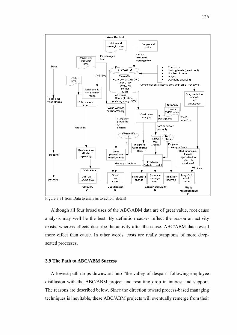
126
Figure 3.31 from Data to analysis to action (detail)
Although all four broad uses of the ABC/ABM data are of great value, root cause
analysis may well be the best. By definition causes reflect the reason an activity
exists, whereas effects describe the activity after the cause. ABC/ABM data reveal
more effect than cause. In other words, costs are really symptoms of more deep-
seated processes.
3.9 The Path to ABC/ABM Success
A lowest path drops downward into “the valley of despair” following employee
disillusion with the ABC/ABM project and resulting drop in interest and support.
The reasons are described below. Since the direction toward process-based managing
techniques is inevitable, these ABC/ABM projects will eventually remerge from their

127
dormant state. Renewed or resurrected ABC/ABM projects can possibly result from
a turnover in managers or too many unplanned surprises, that is, bad and costly
decisions caused by the existing traditional accounting system.
Figure 3.32 Possible paths of ABC/ABM projects (Cokins, 1996)
The middle path reflects strong individuals who continue to champion the virtues
of ABC/ABM thinking. The power of their strong personalities keeps the ABC/ABM
implementation project afloat. Unfortunately, the usefulness of the new cost data
they produce has not been sufficiently recognized by employees to break above that
combustion level for success, where any project or system takes off on its own
merits.
The top path represents the successful ABC/ABM projects that are pulled through
by the unabashed interests of the individuals to use the data to do their jobs better
and make better decisions.
3.10 Causes for ABC/ABM Failures
A good approach is to not repeat mistakes of others and to correct for why many
other ABC/ABM projects have stumbled. Unfortunately, there are so many reasons
that ABC/ABM projects have had difficulties that it is probably more useful to divide
the problems into four broad categories based on the severity (Cokins, 1996):
• The biggies or showstoppers

128
• The user rejections
• The organizational obstacles
• The nuisances
The biggies or showstoppers:
When ABC/ABM projects are launched from the finance or accounting
department, they are usually perceived by those that the project is intended
to help as another meaningless financial or managerial exercise.
Financial accounting tends to be “outside the comfort zone” of most
individuals. The new accounting data cannot be forced upon potential users.
The new ABC/ABM initiative is routinely approached without predefining
tangible, results-oriented objectives. That is, the ABC/ABM model or
system was installed with a “Field of Dreams” illusion as in the recent
Hollywood movie: “if we (the ABC/ABM project team) build it, they (the
data users) will come.” That is nonsense. They won’t come if there were no
problem sets earlier identified for the new data better solve.
There is an impression that simply computing the new ABC/ABM data for
users is a gracious act. Without a plan, even if people look at the data, they
will learn a lot, but they won’t necessarily get anything done.
The ABC/ABM information becomes “a second set of books,” thus
competing with the “official” accounting system. Employee performance
measures are often linked to the official system, which can consequently
encourage bad behaviour.
The magnitude of resistance to change is grossly underestimated. Business
people not trained in financial accounting tend to think a successful
accounting system is one that regularly generates financial reports or that
balances the financial books monthly.
The degree of disbelief of the newly calculated numbers is always
underestimated by the ABC/ABM project team. With accurate tracing of

129
costs, the resulting costs of certain products, services or process outputs can
differ dramatically from their costs as allocated in traditional methods. The
organizational shock is substantial.
Some parties are adversely affected by ABC. For example, product line
managers responsible for products with marginal profitability as calculated
with the traditional allocation data will balk when they recognize that the
ABC calculations can further shift costs into their products and therefore
make their products unprofitable.
The design of the ABC/ABM system is over engineered, excessively
detailed, or flawed in some manner such that the data are not viewed as
useful. Credibility is compromised. The system design flunks the
“closeness beats precision” test too many times. Other flaws include poorly
defining the activities without a verb-noun grammar convention, using too
many activities cost drivers, or not identifying the true cost objects that
consume activities.
Users might reject an ABC/ABM system because of the following:
Sales and marketing personnel do not know how to react nor take
appropriate actions once they are confronted with the new winners and
losers of profitability, whether they are products, services, or customers.
ABC/ABM does not provide all the information for product and customer
planners to make decisions. It simply reflects the disproportionate and
diverse consumption of resources in terms of costs. It sheds little light, for
example, on the potential that customers might bring to future market or
product migration strategies, or where existing products or markets are in
their life cycle.
The ABC/ABM project is viewed as another competing improvement
program rather than as enabling data to aid existing improvements
programs.

130
Acting on the data can involve pain for somebody. The data can lead to
reorganizing people and restructuring their work in different ways that may
eliminate or replace some of the existing people and equipment.
The organizational obstacles to ABC/ABM success:
Brisk pace was not maintained after the ABC/ABM project began. If
ABC/ABM projects take too long, they lose momentum and people lose
interest.
If the pilot site is strictly a cost centre without profit-and-loss responsibility
or not based on market-driven selling prices, people pay less attention.
There is minimal diversity in the number of features of end products or
services.
A higher-level organization unit autocratically mandates ABC/ABM. It
stipulates a predefined, standard set of activity definitions.
ABC/ABM’s reputation as a business improvement tool has been maligned
by naysayers as being too costly or ineffective.
The smaller nuisances affecting ABC/ABM success are:
• The project team leader lacks that “fire in the belly” needed to create
change.
• ABC/ABM training and awareness occurs too early for the eventual internal
users to benefit from. There are insufficient cause-and-effect relationships
between cost flows.
• Activity cost drivers do not adequately reflect the consumption rate and
pattern of their respective activities.
• Hard, measurable data, such as the number of material moves, are
unavailable or inaccessible.
131
CHAPTER FOUR
CASE STUDY
The Industrial Manufacturing Company is considered in this study. We will try to
calculate the unit cost of each product by applying both Traditional and Activity-
Based Costing method. The main aim in this study is to show that Activity-Based
Costing System is better and more accurate than the Traditional Costing System in
estimating the product costs. We will compare the results obtained from by applying
two costing systems.
4.1 The Definition of the Company
The company produces 20 various products in the market. It has the share of 2 %
in the sector. The company has 333 employees in different departments such as
purchasing (2 staffs), warehousing (2 staffs), production (322 staffs, as 313 workers
and 4 engineers and 5 technicians), marketing (1 staff), sales and shipping (2 staffs)
addition to 1 manager, 2 vice-managers and 1 production director. They produce
products in standard specifications and according to customers’ requirements. The
purchasing, production, warehousing, marketing and shipping of all these parts are
the main activity of the company. The company works in a traditional way and all
activities are carried out manually. The company's present costing system is
traditional. There are only three elements of the total cost, direct material cost, direct
labour cost and overhead cost.
The products of the company are respectively P1, P2, P3,…,P20. The monthly
production amount is 89,560 parts. The monthly production amounts of the company
per the product groups, the raw-material costs of the products and also the labour
costs of ones are shown in table 4.1, respectively:
131

132
Table 4.1 The monthly production amount, the raw-material costs, the direct labour costs
P1 P2 P3 P4 P5 P6 P7 P8 P9 P10 P11 P12 P13 P14 P15 P16 P17 P18 P19 P204500 3750 2850 5150 6000 5360 6200 4250 4100 3900 3500 2750 2600 3600 4000 4800 5100 6450 5700 5000
P1 P2 P3 P4 P5 P6 P7 P8 P9 P10 P11 P12 P13 P14 P15 P16 P17 P18 P19 P2018,50 20,25 16,50 15,30 26,40 17,20 28,50 19,50 14,35 21,80 22,60 11,30 13,25 12,45 27,75 23,50 24,30 30,00 29,10 25,50
P1 P2 P3 P4 P5 P6 P7 P8 P9 P10 P11 P12 P13 P14 P15 P16 P17 P18 P19 P208,10 7,50 5,25 3,75 12,50 6,75 14,30 4,80 3,60 9,50 10,25 5,75 6,00 5,35 13,85 9,00 8,25 14,75 13,50 12,00
The monthly production amount
The raw material costs ($)
The direct labour cost ($)
Addition to the company for the manufacturing activity has 50.000 hours-man for
313 manufacturing stuffs and also 20 working days in a month and 8 working hours
in a working day were considered.
The Overhead costs group of the company are machine and building depreciation,
insurance, interest, taxes, advertising, office costs, travel costs, utilities costs, set-up
labour, administrative wages, supplies, material handling, energy costs, indirect
materials, engineering, packing, shipping, maintaining and repair costs.
As the set-up time, the maintaining duration and the repairing duration are
respectively 1250, 3500 and 1500 hours addition to 50,000 hours-man for the
manufacturing.
The manufacturing-related costs of the overhead cost are differently computed in
the costing that are traditional and ABC. Therefore, we considered the costing
systems in different sub-capitals.
4.2 The Calculations in the Cost Systems of the Case Study
Traditional Costing and ABC systems are applied to the accounting.
4.2.1 The Calculations in Traditional Costing System
In this costing system, direct material and labour costs are directly traced as a part
of the cost of the product. Supposed that overhead cost group that was obtained by

133
direct labour costs method is considered as 420% of the direct labour costs. Hence,
we got the overhead costs with 4.2 by multiplying direct labour costs per the product,
respectively. Obtained results are respectively $34.02, $31.50, $22.05, $15.75,
$52.50, $28.35, $60.06, $20.16, $15.12, $39.90, $43.05, $24.15, $25.20, $22.47,
$58.17, $37.80, $34.65, $61.95, $56.70, $50.40. Finding the total overhead cost,
firstly the relative cost by multiplying part number and then the obtained results are
summed. This cost is total overhead cost of the company. The total overhead cost
consists of 19 different cost sub-groups such as machine depreciation, insurance, set-
up labour costs. Previously, each of them was proportioned and was computed by
multiplying the total overhead cost. Obtained results give the costs of overhead cost
group that is shown in table 4.3.
The building depreciation per year was computed by dividing building value
considered scrap rate ($90,658,932.00*0.90 = $81,593,038.80) by life cycle that was
assumed as 30 years. The scrap value was considered as 10% of the building value.
The building depreciation per month was calculated by dividing the one per year
($81,593,038.80/30 = $2,719,767.96) with 12 months ($2,719,767.96/12 =
226,647.33).
The machine depreciation per year was calculated by Incremental Depreciation
technique which depreciation portion value (d) is considered as 1.5 of Straight-line
Depreciation (d = 1.5/n, n: life cycle). The life cycle of machinery is considered 10
years and the present value of them is $48,258,445.56 also, the scrap value at the end
of the life-cycle period is 19.69% of present value. According to Incremental
Depreciation Technique, depreciation value at the end of each year is obtained by
multiplying d (1.5/10 = 0.15) by declining balance. Hence, first-year machine
depreciation value ($48,258,445.56*0.15 ) is $7,238,766.84 and first year value per
month ($7,238,766.84/12 = $603,230.57). Calculating second-year machine
depreciation, by multiplying with the declining balance ($48,258,445.56 -
$7,238,766.84 = $41,019,678.73) and the counting continues respectively.

134
The insurance cost was considered as $41,842.58 according to following equality.
33.81 10
($)12
The building value insuranceThe machine value premiumThe raw material stock rate
The Insurance Cost monthlymonths
−
⎛ ⎞ ⎛ ⎞⎜ ⎟ ⎜ ⎟+ × ×⎜ ⎟ ⎜ ⎟⎜ ⎟ ⎜ ⎟+⎝ ⎠ ⎝ ⎠=
Taken depth is for partially funding in the raw material purchasing that is
$10,460,650. This cost is assigned to the raw material cost, but the interest amount is
a separate cost that is interest cost that was obtained as $87,172.05 (Fund rate
annually = 10%):
($10,460,650) (10%)cos12
depth for the raw material fund
depth interest percentageInterest t monthlymonths
×=
When taxes was counted as $209,212.92 according to following equality:
$41,842,584 6%cos ($)
($)12
Overhead taxest annually rate
Taxes monthlymonths
⎛ ⎞ ⎛ ⎞×⎜ ⎟ ⎜ ⎟
⎝ ⎠ ⎝ ⎠=
The advertising cost was cost as $104,606.46. Office, travel and utilities costs are
respectively $8,717.21, $52,303.23 and $209,212.92.
Set-up labour was considered as $26,151.62 according to following equality:
_ cos($) 1, 250 $ / 20.92
set up set up tSet up labour h h
time monthly per hour−⎛ ⎞ ⎛ ⎞
− = ×⎜ ⎟ ⎜ ⎟⎝ ⎠ ⎝ ⎠
Indirect labour was considered based on traditionally as $69,737.64 according to
following summing:

135
cos ($)
_
Total engineer wages
Indirect labour t monthly Total Technician wages
Total other personnel wages
⎛ ⎞⎜ ⎟+⎜ ⎟⎜ ⎟=⎜ ⎟
+⎜ ⎟⎜ ⎟⎝ ⎠
Administrator wages was considered as $69,737.64 according to following
summing:
min ($)
Pr .
Manager wage
Ad istrator wages monthly Vice managers wages
od Director wage
⎛ ⎞⎜ ⎟+⎜ ⎟⎜ ⎟=⎜ ⎟
+⎜ ⎟⎜ ⎟⎝ ⎠
Following table shows the stuff numbers and wages.
Table 4.2. The stuff numbers and wages
Personnel ManagerVice
ManagerProduction
Director Engineer Technician Worker OtherNumber 1 2 1 4 5 313 7
Wages per stuff $24,000.00 $18,868.82 $8,000.00 $6,000.00 $3,828.00 $16.60/h $3,800.00
The other overhead costs which consist of supplies, material handling, energy
costs, indirect materials, engineering, packing and shipping, maintenance and repairs
shown as in table 4.3.
Supplies cost was counted as $146,449.04 according to following equality:
($) 896 $ / 163.52
100 _
Total CostSupplies monthly orders order o per
number order
A order consists of raw parts
⎛ ⎞ ⎛ ⎞⎜ ⎟ ⎜ ⎟= ×⎜ ⎟ ⎜ ⎟⎜ ⎟ ⎜ ⎟⎝ ⎠ ⎝ ⎠
Material handling cost was counted as $676,455.11 according to following
equality:

136
cos($) 1791.2 $377.66
50
trun number
Material Handling perper month
handling
part number per handling
⎛ ⎞⎛ ⎞ ⎜ ⎟= ×⎜ ⎟ ⎜ ⎟⎝ ⎠ ⎜ ⎟
⎝ ⎠
=
Obtaining the total material cost, the produced products are multiplied by unit
material costs (4500parts*$18.50/part +…+ 5000parts*$25.50/part = $1,963,074.50),
respectively. To find out the total labour cost, the working hours is multiplied by
unit-labour cost per hour (50,000hours*$16.60/hour = $830,210.00) or the produced
products are multiplied by unit-labour cost per product group.
The standard unit costs were calculated by summing of the direct material cost,
the direct labour cost and the overhead cost per part that are shown in table 4.3. The
unit costs from product 1 to product 20 are $60.62, $59.25, $43.80, $34.80, $91.40,
$52.30, $102.86, $44.46, $33.07, $71.20, $75.90, $41.12, $44.45, $40.27, $99.77,
$70.30, $67.20, $106.70, $99.30, $87.90.

137
P1 P2 P3 P4 P5 P6 P7 P8 P9 P10 P11 P12 P13 P14 P15 P16 P17 P18 P19 P20Monthly Production 4500 3750 2850 5150 6000 5360 6200 4250 4100 3900 3500 2750 2600 3600 4000 4800 5100 6450 5700 5000Material cost ($/part) 18,50 20,25 16,50 15,30 26,40 17,20 28,50 19,50 14,35 21,80 22,60 11,30 13,25 12,45 27,75 23,50 24,30 30,00 29,10 25,50
Overhead @ 420% of Direct labour ($/part) 34,02 31,50 22,05 15,75 52,50 28,35 60,06 20,16 15,12 39,90 43,05 24,15 25,20 22,47 58,17 37,80 34,65 61,95 56,70 50,40
Standard unit cost (Traditional costing) ($/part) 60,62 59,25 43,80 34,80 91,40 52,30 102,86 44,46 33,07 71,20 75,90 41,12 44,45 40,27 99,77 70,30 67,20 106,70 99,30 87,90
Energy costs$69.737,64 (2,00%)
$174.344,10
$174.344,10$26.151,62
$146.449,04$676.455,11
$69.737,64
Material handling
$41.842,58$87.172,05
$209.212,92$104.606,46
$8.717,21$52.303,23
$87.172,05 (2,50%)
Repairs $62.763,88$3.486.882,00 (100,00%)
(a)Total labour costs = 50.000 hours * $16,60/hour = $830.210,00
(c)Overhead rate = $3.486.882,00/$830.210,00 = 420%
Office costs
(4,50%)(1,80%)
Indirect Labour
(10,00%)Stockroom space $20.921,29 (0,60%)
$156.909,69
$139.475,28
Advertising
InsuranceInterest
Taxes
$226.647,33
Engineering
Maintenance
Travel costsUtilities costs
Indirect Materials
Supplies
Set-up labour
Monthly Accounting
(b)Total material costs = (4500parts)*($18,50/part) + … + (5000parts)*($25,50/part) = $1.963.074,50
$348.688,20
8,10 7,50 5,25 3,75 12,00
P: Product
5,35 13,85 9,00 8,259,5012,50 3,60 10,25
Overhead
6,75 14,30 4,80
$603.230,59
13,506,005,75Direct labour cost ($/part) 14,75
(5,00%)
(4,00%)
(2,50%)
(17,30%)(6,50%)(1,20%)
(6,00%)(3,00%)(0,25%)(1,50%)
(4,20%)(19,40%)
Total Overhead costs
Total Production Cost = a + b + c Total Production Cost = $6.280.166,5
Machine depreciationBuilding depreciation
Administrative wages
Packing and shipping
(5,00%)(0,75%)(2,00%)
Tablo 4.3 Traditional costing method results
137

138
4.2.2 The Calculations in Activity-Based Costing System
In this costing system, direct material and labour costs are directly traced as a part
of the cost of the product as in traditional costing. However, the overhead costs in
ABC are calculated differently from the ones in traditional costing. Firstly, we
should show that the resources and their costs. The resources in the firm are supplies,
depreciation, building, utilities, energy, stockroom space, indirect materials, indirect
labourers, engineering activities, administrator wages, and other administrating costs
(insurance, interest, advertising, office, travel costs and taxes) and their costs are
$146,449.04, $603,230.57, $226,647.33, $174,344.10, $382,510.95, $20,921.29,
$215,838.00, $759,791.61, $348,688.20, $69,737.64, $503,854.45, respectively and
totally $3,486,882.00. The resources and the costs are shown in table 4.4.
Table 4.4 Resources and the costs
Number Resources Costs1 Supplies $146,449.042 Depreciation $603,230.573 Building $226,647.334 Utilities $174,344.105 Energy $382,510.956 Stockroom space $20,921.297 Indirect materials $215,838.008 Indirect labourers $794,660.439 Engineering activities $348,688.20
10 Adminisrator wages $69,737.64
$3,486,882.00Total
11The sum of Insurance, interest, advertising, office, travel costs,
taxes
$503,854.45
The set-up, supplies, material handling, machine depreciation, building, utilities,
stockroom space, engineering, administrator wages and other costs were explained
and detailed in the traditional costing episode.
Energy cost was counted as $382,510.95 according to following equality:
50,000 ( ) $ / 3.487( cos )cos ($) $5, 230.33 (20% _ cos )
$202,936.53 (30% cos )
h machining hours h energy t per hourEnergy t of set up t
of material handling t
×⎛ ⎞⎜ ⎟= +⎜ ⎟⎜ ⎟+⎝ ⎠

139
Indirect material cost was calculated as $215,838.00 according to following
equality:
50,000 $ / 2.79cos
cos ($) $31,381.94 (20% int cos )$18,829.16 (30% cos )$26,151.62 (30% )
machining indirect materialh h
hours t per hourIndirect material t of ma aining t
of repair tof packing and shipping
⎛ ⎞⎛ ⎞ ⎛ ⎞×⎜ ⎟⎜ ⎟ ⎜ ⎟
⎝ ⎠ ⎝ ⎠⎜⎜= +⎜+⎜⎜+⎝ ⎠
⎟⎟⎟⎟⎟
Indirect labourer cost was calculated as $794,660.43 according to following
equality:
$69,737.64 ( )$20,921.30 (80% _ cos )
$473,518.58 (70% )($)
$125,527.75 (70% int cos )$43,934.72 (70% cos )$61,020.44 (70%
indirect personnel wagesof set up t
of material handlingIndirect labourer
of ma aining tof repair tof pack
++
=+++ )ing and shipping
⎛ ⎞⎜ ⎟⎜ ⎟⎜ ⎟⎜ ⎟⎜ ⎟⎜ ⎟⎜ ⎟⎜ ⎟⎝ ⎠
Machining based on ABC was considered as $1,296,248.37 according to
following equality:
$603, 230.57 (100% cos )$209, 212.92 (100% cos )
cos ($) $169,985.50 (75% )$174,344.10 (50,000 $ / 3.487 " cos ")$139, 475.28 (50,000 $ / 2.
of machine depreciation tof utilities t
Machining t of building depreciationh h energy tsh h
+= +
+ ×+ × 79 " ")indirect materials
⎛ ⎞⎜ ⎟⎜ ⎟⎜ ⎟⎜ ⎟⎜ ⎟⎜ ⎟⎝ ⎠
Inventory cost was counted as $54,918.39 according to following equality:
$20,921.29 (100% )cos ($)
$33,997.10 (15% )of stockroom space
Inventory tof building depreciation
⎛ ⎞= ⎜ ⎟+⎝ ⎠
Control cost was calculated as $139,475.28 according to following equality:

140
$69,737.64 (100% min cos )cos ($)
$69,737.64
of ad istrator tControl t the sum of indirect
personnel wages
+⎛ ⎞⎜ ⎟= ⎛ ⎞⎜ ⎟+ ⎜ ⎟⎜ ⎟⎝ ⎠⎝ ⎠
Packing and shipping cost was counted as $87,172.05 according to following
equality:
cos ($) $ / 0.9733 cos 89,560packing and
total productionPacking and shipping t p shipping t p
amount monthlyper product
⎛ ⎞⎛ ⎞⎜ ⎟= × ⎜ ⎟⎜ ⎟ ⎝ ⎠⎜ ⎟
⎝ ⎠
Maintaining cost was considered as $156,909.69 according to following equality:
int intint cos ($) 3,500 $ / 44.83
cosma aining ma aining
Ma aining t h hhours t per hour
⎛ ⎞ ⎛ ⎞= ×⎜ ⎟ ⎜ ⎟
⎝ ⎠ ⎝ ⎠
Repair cost was counted as $85,428.61 according to following equality:
cos1,500 $ / 41.843
Re cos ($)$22,664.73 (10% )
total repair repair th h
pair t hours per hoursof building depreciation
⎛ ⎞⎛ ⎞ ⎛ ⎞×⎜ ⎟⎜ ⎟ ⎜ ⎟= ⎝ ⎠ ⎝ ⎠⎜ ⎟
⎜ ⎟+⎝ ⎠
Secondly, we show that which activity consumes which resource. The activities in
the firm are set-up, orders, machining, material handling, inventory, maintaining,
repairs, control, engineering, packing and shipping, other administrating costs,
respectively. Also, the resources consumed by activities are shown in table 4.5.
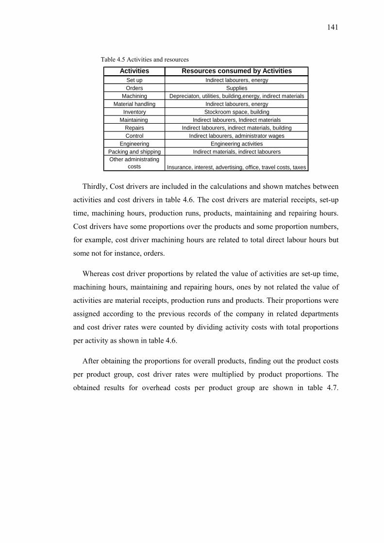
141
Table 4.5 Activities and resources
Activities Resources consumed by ActivitiesSet up Indirect labourers, energyOrders Supplies
Machining Depreciaton, utilities, building,energy, indirect materialsMaterial handling Indirect labourers, energy
Inventory Stockroom space, buildingMaintaining Indirect labourers, Indirect materials
Repairs Indirect labourers, indirect materials, buildingControl Indirect labourers, administrator wages
Engineering Engineering activitiesPacking and shipping Indirect materials, indirect labourersOther administrating
costs Insurance, interest, advertising, office, travel costs, taxes
Thirdly, Cost drivers are included in the calculations and shown matches between
activities and cost drivers in table 4.6. The cost drivers are material receipts, set-up
time, machining hours, production runs, products, maintaining and repairing hours.
Cost drivers have some proportions over the products and some proportion numbers,
for example, cost driver machining hours are related to total direct labour hours but
some not for instance, orders.
Whereas cost driver proportions by related the value of activities are set-up time,
machining hours, maintaining and repairing hours, ones by not related the value of
activities are material receipts, production runs and products. Their proportions were
assigned according to the previous records of the company in related departments
and cost driver rates were counted by dividing activity costs with total proportions
per activity as shown in table 4.6.
After obtaining the proportions for overall products, finding out the product costs
per product group, cost driver rates were multiplied by product proportions. The
obtained results for overhead costs per product group are shown in table 4.7.

142
P1 P2 P3 P4 P5 P6 P7 P8 P9 P10 P11 P12 P13 P14 P15 P16 P17 P18 P19 P204500 3750 2850 5150 6000 5360 6200 4250 4100 3900 3500 2750 2600 3600 4000 4800 5100 6450 5700 5000
Orders $146.449,04 Material receipts 45 37,5 28,5 51,5 60 53,6 62 42,5 41 39 35 27,5 26 36 40 48 51 64,5 57 50 895,60 163,52Set up $26.151,62 Set-up time (hours) 40 37 55 75 45 80 83 51 47 64 62 52 76 82 74 64 81 90 49 43 1250,00 20,92
Machining $1.261.379,55 Machining hours 2020 2750 2070 2875 2885 2495 2935 2345 2015 1980 1800 2385 2155 2670 2225 2725 2595 3245 3030 2800 50000,00 25,23Material handling $676.455,11 Production runs 90 75 57 103 120 107,2 124 85 82 78 70 55 52 72 80 96 102 129 114 100 1791,20 377,66
Inventory $54.918,39 Products 45 37,5 28,5 51,5 60 53,6 62 42,5 41 39 35 27,5 26 36 40 48 51 64,5 57 50 895,60 61,32Maintaining $156.909,69 Maintaining hours 200 175 155 235 265 245 280 140 115 100 95 85 90 110 135 150 185 300 210 230 3500,00 44,83
Repairs $85.428,61 Repairing hours 80 62 67 80 100 94 115 65 45 44 48 43 51 52 58 76 88 135 96 101 1500,00 56,95Control $139.475,28 Products 5,86 4,39 3,63 6,28 7,21 5,96 7,50 5,04 5,45 4,16 3,39 2,52 2,23 3,63 4,16 4,80 4,92 6,74 5,92 6,21 100,00 1.394,75
Engineering $348.688,20 Engineering rate 5,50 3,75 3,25 4,85 6,05 5,70 6,20 5,40 5,00 4,80 4,25 3,10 2,90 4,60 4,20 4,95 6,05 7,50 6,90 5,05 100,00 3.486,88Packing and shipping $87.172,05 Products 5,02 4,20 3,19 5,75 6,70 5,98 6,92 4,75 4,58 4,35 3,91 3,07 2,90 4,02 4,47 5,36 5,69 7,20 6,36 5,58 100,00 871,72
Products 3,75 3,557,05 3,357,40 3,90
Activities Cost Cost Drivers
Other administrating costs $503.854,45 2,90 3,45 5,00 5,804,30 3,056,253,85 3,60 6,15
Cost Driver Rates
5.038,55100,006,40 7,00 6,70
Total
6,55
Table 4.6 Activity costs and their allocation to products
142

143
Obtaining the unit costs per product group, firstly total direct material and labour
cost were separately counted by multiplying direct material cost and direct labour
cost with total product amount per product group. The results were summed with
overhead total costs, respectively and total production cost was obtained.
The unit costs per product group according to activity-based costing were
computed by dividing total production cost with total product number per product
group. The obtained results are shown in table 4.7.
As seen, the obtained unit costs according to traditional costing are different from
the ones according to ABC. This difference takes place because of different
computing method of ABC and traditional costing.
Activity based costing method with more reasonable way can compute the
product costs closing the actual, since overhead costs are assumed as a part of
operating cost via activities, cost driver and cost driver rates.

144
Direct Material ($/part) 18,50 20,25 16,50 15,30 26,40 17,20 28,50 19,50 14,35 21,80Direct Labour ($/part) 8,10 7,50 5,25 3,75 12,50 6,75 14,30 4,80 3,60 9,50
Total Direct Material ($) 83250,00 75937,50 47025,00 78795,00 158400,00 92192,00 176700,00 82875,00 58835,00 85020,00Total Direct Labour ($) 36450,00 28125,00 14962,50 19312,50 75000,00 36180,00 88660,00 20400,00 14760,00 37050,00
Overhead ($)Orders 7358,40 6132,00 4660,32 8421,28 9811,20 8764,67 10138,24 6949,60 6704,32 6377,28Set up 836,80 774,04 1150,60 1569,00 941,40 1673,60 1736,36 1066,92 983,24 1338,88
Machining 50959,73 69375,87 52221,10 72529,32 72781,59 62942,84 74042,98 59158,70 50833,59 49950,62Material handling 33988,95 28324,13 21526,34 38898,47 45318,60 40484,62 46829,22 32100,68 30967,71 29457,09
Inventory 2759,40 2299,50 1747,62 3157,98 3679,20 3286,75 3801,84 2606,10 2514,12 2391,48Maintaining 8966,20 7845,43 6948,81 10535,30 11880,20 10983,60 12552,70 6276,34 5155,57 4483,10
Repairs 4556,16 3531,02 3815,78 4556,16 5695,20 5353,49 6549,48 3701,88 2562,84 2505,89Control 8173,25 6122,96 5062,95 8759,04 10056,17 8312,73 10460,65 7029,55 7601,40 5802,17
Engineering 19177,85 13075,81 11332,37 16911,38 21095,64 19875,23 21618,67 18829,16 17434,41 16737,03Packing and shipping 4376,03 3661,23 2780,79 5012,39 5840,52 5212,89 6032,30 4140,67 3992,48 3791,98
Other administrating costs 21665,77 19398,42 18138,78 30987,08 35521,78 31490,94 37285,27 19650,35 18894,56 17886,85
Total Overhead ($) 162818,54 160540,41 129385,46 201337,40 222621,50 198381,36 231047,71 161509,95 147644,24 140722,37
Total Production Cost ($) 282518,54 264602,91 191372,96 299444,90 456021,50 326753,36 496407,71 264784,95 221239,24 262792,37Total Product Number ($) 4500 3750 2850 5150 6000 5360 6200 4250 4100 3900
The Unit Cost (ABC) ($/part) 62,78 70,56 67,15 58,14 76,00 60,96 80,07 62,30 53,96 67,38
P7 P8 P9 P10Activities P1 P2 P3 P4 P5 P6
Table 4.7a Activity-based costing for the products
144

145
Direct Material ($/part) 22,60 11,30 13,25 12,45 27,75 23,50 24,30 30,00 29,10 25,50Direct Labour ($/part) 10,25 5,75 6,00 5,35 13,85 9,00 8,25 14,75 13,50 12,00
Total Direct Material ($) 79100,00 31075,00 34450,00 44820,00 111000,00 112800,00 123930,00 193500,00 165870,00 127500,00 1963074,50Total Direct Labour ($) 35875,00 15812,50 15600,00 19260,00 55400,00 43200,00 42075,00 95137,50 76950,00 60000,00 830210,00
Overhead ($)Orders 5723,20 4496,80 4251,52 5886,72 6540,80 7848,96 8339,52 10547,04 9320,64 8176,00 146448,51Set up 1297,04 1087,84 1589,92 1715,44 1548,08 1338,88 1694,52 1882,80 1025,08 899,56 26150,00
Machining 45409,66 60167,80 54365,46 67357,66 56131,39 68745,18 65465,60 81863,53 76439,60 70637,25 1261379,47Material handling 26435,85 20771,03 19638,06 27190,80 30212,00 36254,40 38520,30 48716,85 43052,10 37765,00 676452,20
Inventory 2146,20 1686,30 1594,32 2207,52 2452,80 2943,36 3127,32 3955,14 3495,24 3066,00 54918,19Maintaining 4258,95 3810,64 4034,79 4931,41 6052,19 6724,65 8293,74 13449,30 9414,51 10311,10 156908,53
Repairs 2733,70 2448,94 2904,55 2961,50 3303,22 4328,35 5011,78 7688,52 5467,39 5752,15 85428,00Control 4728,21 3514,78 3110,30 5062,95 5802,17 6694,81 6862,18 9400,63 8256,94 8661,42 139475,26
Engineering 14819,25 10809,33 10111,96 16039,66 14644,90 17260,07 21095,64 26151,62 24059,49 17608,75 348688,22Packing and shipping 3408,43 2676,18 2527,99 3504,32 3896,59 4672,42 4960,09 6276,38 5544,14 4864,20 87172,02
Other administrating costs 16879,14 15367,58 14611,80 17383,00 25192,75 29223,59 32246,72 35269,85 33758,29 33002,50 503855,02
Total Overhead ($) 127839,63 126837,22 118740,67 154240,98 155776,89 186034,67 195617,41 245201,66 219833,42 200743,93 3486875,42
Total Production Cost ($) 242814,63 173724,72 168790,67 218320,98 322176,89 342034,67 361622,41 533839,16 462653,42 388243,93 6280159,92Total Product Number ($) 3500 2750 2600 3600 4000 4800 5100 6450 5700 5000 89560
The Unit Cost (ABC) ($/part) 69,38 63,17 64,92 60,64 80,54 71,26 70,91 82,77 81,17 77,65 -
-
TotalActivities P11 P12 P13 P14 P19 P20P15 P16 P17 P18
Table 4.7b Activity-based costing for the products (continue).
145

146
4.3 The Comparing of Two Costing Systems
The unit costs by computed Traditional and Activity Based Costing are shown in
the table 4.8. The following table also shows difference amount and percentage
between unit costs of traditional costing and ABC. According to ABC system, over-
cost products in following table are P5, P7, P10, P11, P15, P18, P19, P20, whereas under-
cost products in the same table are P1, P2, P3, P4, P6, P8, P9, P12, P13, P14, P16, P17 as
showed.
Table 4.8 Comparing traditional costing and activity based costing unit costs P1 P2 P3 P4 P5 P6 P7 P8 P9 P10
Traditional Costing ($) 60,62 59,25 43,80 34,80 91,40 52,30 102,86 44,46 33,07 71,20
Activity Based Costing ($) 62,78 70,56 67,15 58,14 76,00 60,96 80,07 62,30 53,96 67,38
Difference ($) 2,16 11,31 23,35 23,34 -15,40 8,66 -22,79 17,84 20,89 -3,82
Difference Percentage (%) 3,56% 19,09% 53,31% 67,07% -16,85% 16,56% -22,16% 40,13% 63,17% -5,37%
P11 P12 P13 P14 P15 P16 P17 P18 P19 P20
Traditional Costing ($) 75,90 41,12 44,45 40,27 99,77 70,30 67,20 106,70 99,30 87,90
Activity Based Costing ($) 69,38 63,17 64,92 60,64 80,54 71,26 70,91 82,77 81,17 77,65
Difference ($) -6,52 22,05 20,47 20,37 -19,23 0,96 3,71 -23,93 -18,13 -10,25
Difference Percentage (%) -8,59% 53,62% 46,05% 50,58% -19,27% 1,37% 5,52% -22,43% -18,26% -11,66%
If the traditional costing values are shown the fluctuations of the ABC values can
also be plotted as can be seen in figure 4.1 and 4.2.
Figure 4.1 The comparison scatter chart of two costing methods

147
Figure 4.2 The comparison colum
n chart for two costing m
ethods
147

148
Results of the two costing systems were different in computing the unit product
costs. The present cost system that was used by the managers accepted the
production amount as the measure in the charging of indirect activities on to
products. Every product is not been possible to consume resources at the same rate. It
was clearly understood that it is necessary to charge indirect costs on to every
product in different rates while research and studies related to ABC were being
made.
4.4 Conclusion
In this thesis, the importance and the necessity of the application of the ABC
system in product costing have been emphasized. It has also been pointed out that
obtained costing information by used traditional costing is not correct and reliable in
the companies. Consequently, the ABC system has been developed because
traditional costing systems lead to misinformation in product costing. Because
costing information affects the decisions of the managers about marketing, costing
and selling, the correct costing system is vitally important for the companies. It is
inevitable that the companies incur losses if inaccurate cost information like
traditional costing method is used. Therefore, a trustworthy costing method like
activity based costing is vitally important for the companies.
When the course of ABC’s development is examined, the system can be seen to
have gone through some various stages until now. It was at first used to reach correct
product costing, but nowadays it is being used for different purposes. The ABC
system is applied successfully not only in the production sector but also in the
service sector as well.
In chapter one of the thesis, literature review has ABC applications in various
fields which are manufacturing and service sectors. In chapter two, traditional
costing methods with some case studies were examined, and following chapter
presented ABC which is main focus in the study. Clarifying what ABC, ABM, the
method, various business improvements approaching, implementation stages, causes
for ABC, ABM failure and the path to ones success were detailed and examined. The

149
last chapter presents the case study of the thesis. In this chapter, a manufacturing
company was examined by traditional costing and ABC methods. Firstly, the product
costs were calculated based on traditional costing system which allocates overhead
costs to products and the results were showed in table 4.3. Secondly, the product
costs were calculated based on ABC which assigns the overhead costs to products via
cost driver and the results were presented in table 4.7. Two results obtained from
application of traditional costing and ABC system were compared in table 4.8 and
figure 4.1, graphically. The cost data in table 4.8 presents based on ABC system
over-cost and under-cost products. According to ABC system, over-cost products are
P5, P7, P10, P11, P15, P18, P19, P20 which took place hidden-profit, whereas under-cost
products are P1, P2, P3, P4, P6, P8, P9, P12, P13, P14, P16, P17 which took place hidden
loss. Over-cost products present more costing than the normal costs, whereas under-
cost products present less costing than the normal costs.
It is inevitable to come across some obstacles in the companies no matter where
the ABC system is applied. The reasons of these obstacles can be categorized into
two main groups. Firstly, the difficulties occur due to the selected scientific method.
The executives are highly sensitive about secrecy and are not sympathetic to studies
related to this subject especially when the information is cost related. Secondly, the
ABC system requires sensitive computations, deep analysis and detailed information
because of its structure. Acquisition of the information necessary for the completion
of an ABC system can be quite costly in terms of both time and task force.
At the end of the application, the research and reviews of opinion that the ABC
system is more useful and will give more reliable results has been reached. Because
it presents valuable information, except for the unit costs of products, to managers, it
provides the possibility to identify, solve and prevent the problem about
effectiveness of the activity and the cost control, especially by identifying the costing
of the activity. It gives detailed information about the organizational form of the
company and production process.
ABC system facilitates a departmental assessment of the company, an effective
cost control, and the measurement of the effectiveness of every activity that takes
place in it. Therefore, it is understood that ABC can be used as a strategic

150
management instrument. Also, by taking the recent studies into consideration, this
system can be used with different techniques (TQM, BPR, etc.). In this respect, the
techniques which were not used in the past can be determined and the suitable ones
can be used with the ABC system.

151
References
Activity Based Costing. (n.d.). Retrieved April 6, 2009, from
http://en.wikipedia.org/wiki/Activity-based_costing
Baykasoğlu, A. & Kaplanoğlu, V. (2008). Application of activity-based costing to a
land transportation company: A case study. Elsevier, pp 308-324
Beck, U., & Nowak, J.W. (2000). The Merger of Discrete Event Simulation with
Activity Based Costing for Cost Estimation in Manufacturing Environments.
Proceedings of the 2000 Winter Simulation Conference in U.S.A.
Blossom Yen-Ju Lin, Te-Hsin Chao, Yuh Yao, Shu-Min Tu, Chun-Ching Wu, Jin-
Yuan Chern, Shiu-Hsiung Chao, & Keh-Yuong Shaw, (2007). How Can Activity-
Based Costing Methodology Be Performed as a Powerful Tool to Calculate Costs
and Secure Appropriate Patient Care. Springer Science+Business Media, Inc.
Carles Griful-Miquela, (2001). Activity-Based Costing Methodology for Third-Party
Logistics Companies. International Advances in Economic Research
Chabrol, M., Chauvet, J., Féniès, P., & Gourgand M., (2006). A Methodology for
Process Evaluation and Activity Based Costing in Health Care Supply Chain. pp.
375 – 384, Springer-Verlag Berlin Heidelberg
Chih-Wei, Jeremy, & Li, C.M.Cheng. (2008). Monitor Cost Reduction through
Application of Activity Based Costing, Taiwan
Cokins, G., (1996). Activity Based Cost Management. The United States of America;
McGraw-Hill Companies ISBN 0-7863-0740-4
Eski, H., & Armaneri, Ö., (2006). Mühendislik Ekonomisi. Turkey: Gazi Kitabevi.
ISBN 975-6009-68-3

152
Fichman R. G., & Kemerer, C. F., (2002). Activity Based Costing for Component-
Based Software Development. Information Technology and Management 3.
Kluwer Academic Publishers. pp. 137–160,
Gunasekaran, A. & Singh D., (1999). Design of Activity-Based Costing in a Small
Company: A Case Study. Pergamon, Pages 413-416
Gupta, A., Stahl, D.O., & Whinston, A.B., (1997). A Decentralized Approach to
Estimate Activity-Based Costs and Near-Optimal Resource Allocation in Flexible
Manufacturing Systems. The International Journal of Flexible Manufacturing
Systems. Kluwer Academic Publishers, 167–193
Hirsch, M.L., & J.G., (1986). Cost Accounting: Accumulation, Analysis, and Use.
The United States of America; Kent Publishing Company ISBN 0-534-05970-8
Homburg, C. (2004). Improving activity-based costing heuristics by higher-level cost
drivers. European Journal of Operational Research, Volume 157, pp. 332-343
Horngren, Charles T., Foster, G., & Dator, Srikant M. (2001). Cost Accounting: A
Managerial Emphasis, Stanford University & Harvard University, New Jersey,
USA: Tenth Edition, Printice Hall Inc., ISBN 81-203-1707-6
Iltuzer, Z., Tas, O. & Gozlu, S., (2007). Implementation of Activity-Based Costing in
e-Businesses, Turkey PICMET Proceedings, pp. 123-132
Işık, A., (2000). Mühendislik Ekonomisi. Turkey; Bizim Büro Basımevi, ISBN 975-
8201-13-1
Januszewski, Arkadiusz., (2005). Activity Based Costing System for a Medium sized
Trade Company. Springer, “Advances in Information Systems Developments”, pp.
349-358

153
Jun, T., & Zhongchuan L., (2002). Study on IT Service Cost’s Calculate and
Charging Strategy Based on Activity-based Costing, International Journal
of Production Economics, Vol. 5, pp. 71-82
Kaplan, Robert S., & Bruns, W. (1987). Accounting and Management: A Field Study
Perspective. USA; Harvard Business School Press, ISBN 0-87584-186-4
Kataoka, T., Kimura, A., Morikawa, K., & Takahashi, K., (2007). Integrating
Activity Based Costing and Process Simulation for Strategic Human Planning.
Springer, pp. 273-280
Katz, David M. (2002). Activity-Based Costing (ABC): In recent years, ABC has lost
ground in the metric wars. But it may be set for a resurgence. Retrivied
November 12, 2009, from http://www.cfo.com/article.cfm/3007694
Lee, John Y. (2002). An Examination of International Differences in Adoption and
Theory Development of Activity-Based Costing. Advances in International
Accounting, Volume 15, pages 65-77, Elsevier Science Ltd., ISBN: 0-7623-0952-
0
Liu W., Xiao L., Zhang J., Feng Y. & Zeng M. (2008). The Design of Activity-based
Costing Model for Guohua Electric Power Company. IEEE Xplore.
Narita, H., Chen, L., & Fujimoto, H., Cost Prediction System Using Activity-Based
Model for Machine Tool Operation. Springer IFIP International Federation for
Information Processing, pp. 399-407
Okka, O., (2000). Mühendislik Ekonomisi. Turkey: Nobel Yayın Dağıtım Ltd. Şti.
ISBN 975-591-123-5

154
Park, J. & Simpson, & Timothy W. (2005). An Activity-Based Costing Method to
Support Product Family Design. International Journal of Production Research,
Volume 43, pp. 731 - 772
Qian, Li. and Ben-Arieh, David (2007). Parametric cost estimation based on activity-
based costing: A case study for design and development of rotational parts.
International Journal of Production Economics, volume 113, pp. 805-818
Rasmussen, Rodney R., Savory, Paul A., & Williams, Robert E. (1999). Integrating
simulation with activity-based management to evaluate manufacturing cell part
sequencing. Computers & Industrial Engineering volume 37, Issue 4, 1999, pp.
757-768
Raz, T. & Elnathan, D. (1999). Activity based costing for projects. International
Journal of Project Management Vol. 17, No. 1, pp. 61-67, Great Britain.
Ridderstolpe, L., Johansson, A., Skau T., Rutberg, H. & Ahlfeldt, H. (2002). Clinical
Process Analysis and Activity-Based Costing at a Heart Centre. Journal of
Medical Systems, Vol. 26, pp. 309-322
Rocha , L. S., & Bassani, J. W. M., (2004). Cost Management of Medical Equipment
Maintenance. Proceedings of the 26th Annual International Conference of the
IEEE EMBS
Sapp, R., Crawford, D., & Rebishcke, S. (1990). Journal of Bank Cost and
Management Accounting, Volume 3, Number 2, pp. 53-62
Sun Yi-ran, Zhao Song-zheng, Liu Wei, & XU Heng. (2007). Research on a
Manufacturing Cost Estimating Method Based on ABC for Aeronautic Product,
IEEE Explore

155
Sundin, E., & Tyskeng, S., (2003). Refurbish or Recycle Household Appliances? An
Ecological and Economic study of Electrolux in Sweden. Division of Production
Systems. Proceedings of EmDesign2003 Third International Symposium on
Environmentally Conscious Design and inverse Manufacturing
Tuncel, G., Akyol, D., Bayhan, Gunhan M., & Koker, U. (2005). Application of
Activity-Based Costing in a Manufacturing Company: A Comparison with
Traditional Costing. Springer-Verlag Berlin Heidelberg, pp. 562–569.
Yi-Chun Tsai, & lung-Sheng Jao., (2002). Activity-Based Costing Application in
Indirect Material Cost Control -Photo-resist; Taiwan Semiconductor
Manufacturing Company Ltd: Science-Based lndustrial Park Hsin-Chu