actuator and sensor placement in linear advection pde with...
TRANSCRIPT
Actuator and sensor placement in linear
advection PDE with building systems
application
U. Vaidya b,1 R. Rajaram a and S. Dasgupta c
aDepartment of Math. Sci., 3300, Lake Rd West, Kent State University, Ashtabula, OH - 44004
bDept. of Elec. and Comp. Engg., Iowa State University, Ames, IA 50011, Email: [email protected]
cDept. of Elec. and Comp. Engg., Iowa State University, Ames, IA 50011, Email:
Abstract
We study the problem of actuator and sensor placement in a linear advection partial
differential equation (PDE). The problem is motivated by its application to actuator
and sensor placement in building systems for the control and detection of a scalar
quantity such as temperature and contaminants. We propose a gramian based ap-
proach to the problem of actuator and sensor placement. The special structure of the
advection PDE is exploited to provide an explicit formula for the controllability and
observability gramian in the form of a multiplication operator. The explicit formula
for the gramian, as a function of actuator and sensor location, is used to provide test
criteria for the suitability of a given sensor and actuator location. Furthermore, the
solution obtained using gramian based criteria is interpreted in terms of the flow of
the advective vector field. In particular, the almost everywhere stability property of
the advective vector field is shown to play a crucial role in deciding the location of
actuators and sensors. Simulation results are performed to support the main results
of this paper.
Preprint submitted to Elsevier 1 December 2011
Key words: Controllability and observability gramians, Advection Equation,
Building systems
PACS: 93D05, 93B07
1 Introduction
In this paper, we study the problem of actuator and sensor placement in a
linear advection partial differential equation. The problem is motivated by
its application to actuator and sensor location in building systems for the
purpose of control of temperature and detection of contaminants. Building
systems in US account for 39 percent of total energy consumption [1]. Design
of efficient building systems not only has a significant economic benefit but
also social and environmental benefits. Social benefits arise due to improved
overall quality of life by enhancing occupant health, comfort and heightened
aesthetic qualities. Improvement in water and air quality and reduced waste
lead to environmental benefits.
The optimal placement of actuators and sensors in a building system is a
difficult problem due to the complex physics that is involved. The governing
equations for building system fluid flows and scalar densities are coupled non-
linear partial differential equations subjected to disturbances, various sources
of uncertainties, and complicated geometry. Analysis of the building system
with its full scale complexity leads to a finite element based computational
approach to the actuator and sensor placement problem [2]. Such a purely
computational based approach provides little insight into the obtained solu-
1 Corr. author Email: [email protected]
2

tion. An alternate system theoretic and dynamical systems based approach
under some simplifying assumptions and physics can also be pursued [3,4].
Such an approach provides useful insights and guidelines to the complex con-
trol problems involved in building system applications. In this paper, we pur-
sue a similar approach for the location of actuators and sensors problem in a
building system.
Under some simplifying assumptions and physics [3,4], the system equations
are modeled in the form of a linear advection partial differential equation with
inputs and outputs. We propose a gramian based approach to the actuator
and sensor location problem. The results are an important first step towards
its application to building systems. However, further research needs to be done
for relaxing some of the simplifying assumptions made in this paper for the
applicability of these results for the building systems problem. We believe that
the analytical methods developed in this paper combined with computational
techniques involving detailed physics of building systems is a right approach
moving forward. The main contribution of this paper is in providing explicit
formula for the controllability and observability gramians as a function of ac-
tuator and sensor locations and the advection velocity field. These explicit
formulas for the gramians are used to provide test criteria for deciding the
location of sensors and actuators. Technical conditions for the existence of in-
finite time gramians are also provided. In particular, we prove that the infinite
time controllability and observability gramians are well defined for almost ev-
erywhere stable and asymptotically stable advection vector fields respectively.
We provide simulation results using a two dimensional fluid flow vector field for
the computation of the finite time controllability and observability gramian.
An excellent review and classification of sensor and controller positioning for
3

distributed parameter systems can be found in [5], where most of the methods
involve a finite dimensional approximation of the infinite dimensional system,
either before or after solving an optimization problem using the point spectrum
of the infinitesimal generator. It was noted in [5] that such an approximation
based method will not work for wave type systems because of the finite speed
of propagation. [6] is an excellent book on sensor and actuator placement for
distributed parameter systems governed by heat and diffusive type processes.
[7] describes sensor and actuator placement for flexible structures. A combina-
torial optimization approach for linear time invariant systems based on integer
programming using the controllability and observability gramians for sensor
and actuator placement can be found in [8].
The linear advection equation considered in this paper is akin to a unidirec-
tional wave equation whose wave speed is governed by a nonlinear smooth
vector field f(x). Hence, actuator and sensor placement analysis based on a
finite dimensional approximation as developed in earlier references will not
work well for our problem. Our selection criteria for actuators and sensors
uses the idea of controllability and observability gramians, but differs from
what is seen in the literature slightly. The advection equation has a funda-
mental limitation for control as described in Theorem (5), in the sense that
placing an actuator on the set B can only affect states ρ whose support is
RτB = ∪τt=0φt(B). This set Rτ
B is precisely the support of the controllability
gramian CτB for the advection equation (see Claim (8)). This is the main reason
why we consider choosing a set B for actuators that maximizes the support
of CτB. For sets B that give the same support for CτB, we choose the one that
gives lesser L2 norm, since that will minimize the control effort (see Theorem
(5), where the minimum norm control formula has the controllability gramian
4

appearing in the denominator).
The organization of the paper is as follows. In section 2, we describe the prob-
lem and some preliminaries from the theory of partial differential equations.
In section 3, we present the main results of the paper. In section 4, we discuss
technical conditions for the existence of the infinite time controllability and
observability gramians. Simulation results are presented in section 5 followed
by conclusion in section 6.
2 Preliminaries
We study the problem of optimal location of actuator in a linear advection
partial differential equation. The motivation for this problem comes from the
optimal location of actuators for the control of a scalar quantity, such as
temperature or contaminants, in a room denoted by ρ(x, t).
In building system applications, the evolution of ρ(x, t), is governed by the
velocity field v(x, t) of the fluid flow. This velocity field is obtained as a solution
of the following Navier Stokes equation:
∂v(x, t)
∂t+ v(x, t) · ∇v(x, t) = −∇p(x, t) +
1
Re4 v(x, t)
∇ · v(x, t) = 0, (1)
where x ∈ X ⊂ RN (with N = 2 or 3) is the domain of the room, v(x, t)
is the velocity field, p(x, t) is the pressure, and Re is the Reynolds number.
The evolution of the scalar quantity ρ(x, t) is governed by the following linear
controlled partial differential equation
5

∂ρ
∂t+ v(x, t) · ∇ρ(x, t) =
1
PrRe4 ρ(x, t) +
N∑k=1
χBk(x)uk(t)
yk(x, t) =χAk(x)ρ(x, t), k = 1, . . . ,M (2)
where Pr is the Prandtl number, χAk(x) is the indicator function on set Ak ⊂
X, and uk(t) ∈ R is the control input for k = 1, . . . , N . The form of control
input χB(x)u(t) and output measurement χA(x)ρ(x, t) is motivated by the
fact that the actuation and sensing can be exercised only on a small region B
and A of the physical space X respectively.
Remark 1 The form of output equation in (2) is different than the one usu-
ally considered in the literature, where the sensors have access to the average
state information on a set (i.e., yk(t) =∫Akck(x)ρ(x, t)). The interpretation
in our case is that the sensors have pointwise state information from the sets
Ak. We choose the form in (2) because it allows us to compute the observabil-
ity gramians as a explicit function of section location set Ak. Our proposed
approach can also be applied to the case where the sensors have access to av-
erage state information, however, the observability gramian in that case will
be a complicated function of the sensor location set Ak. Furthermore this form
of output measurement is also dual to the input actuation term, in particular
to Eq. (4).
The objective is to determine the optimal location of actuators and sensors,
and hence the determination of indicator function χBk(x) and χAk(x). The
terms v(x, t) · ∇ρ(x, t) and 4ρ(x, t) in (2) correspond to advection and diffu-
sion respectively, with D = 1RePr
being the diffusion constant. Note that the
advection diffusion equation (2) is decoupled from the Navier Stokes equation
(1). In the case where the scalar density is temperature, this decoupling cor-
responds to the assumption that buoyancy forces have negligible or no effect.
6

Furthermore, for simplicity of presentation of the main results of this paper,
we now make the following assumptions.
Assumption 2 We replace the time varying velocity field v(x, t) responsible
for the advection of scalar density with the mean velocity field f(x) i.e.,
f(x) :=1
T
∫ T
0v(x, t)dt
Remark 3 Typically the velocity field information v(x, t) is available over
a finite time interval [0, T ] either from a simulation or from an experiment.
Assumption (2) corresponds to linearizing the linear advection PDE along the
mean flow field f(x). It follows that if v(x, t) is volume preserving i.e., ∇ ·
v(x, t) = 0, then ∇ · f(x) = 0 as well.
Assumption 4 Again for simplicity of presentation of the main results of
this paper, we assume that the diffusion constant D in the advection diffusion
equation (2) is zero. As we see in the simulation section, the assumption of
zero diffusion constant is justified.
We next discuss a few preliminaries on semigroup theory of partial differential
equations. Consider the following ordinary differential equation (ODE):
x = f(x), x(0) = x0, (3)
where x ∈ X ⊂ RN a compact set. We denote by φt(x) the solution of ODE
(3) starting from the initial condition x. ODE (3) is used to define two linear
infinitesimal operators, AK : L2(X) → L2(X) and APF : L2(X) → L2(X)
defined as follows:
AKρ = f · ∇ρ, APFρ = −∇ · (fρ).
7

The domains of the above operators are given as follows:
D(AK) = {ρ ∈ H1(X) : ρ|Γo = 0},
D(APF ) = {ρ ∈ H1(X) : ρ|Γi = 0},
where Γo and Γi are the outflow and inflow portions of the boundary ∂X
defined as follows:
Γo = {x ∈ ∂X : f · η > 0}, Γi = {x ∈ ∂X : f · η < 0},
where η is the outward normal to the boundary ∂X. The semigroups cor-
responding to the AK and APF are called as Koopman (Ut) and Perron-
Frobenius (Pt) operators respectively. These operators are defined as follows:
Ut : L2(X)→ L2(X), (Utρ)(x) = ρ(φt(x)),
Pt : L2(X)→ L2(X), (Ptρ)(x) = ρ(φ−t(x))
∣∣∣∣∣∂φt(x)
∂x
∣∣∣∣∣−1
,
where | · | denotes the determinant. These semigroups can be shown to satisfy
the following partial differential equations [9]:
∂ρ
∂t−AKρ = 0, ρ|Γo = 0;
∂ρ
∂t−APFρ = 0, ρ|Γi = 0.
The Koopman and Perron-Frobenius semigroup operators and their infinites-
imal generators are adjoint to each other i.e.,
∫X
(Ptρ1)(x)ρ2(x)dx =∫Xρ1(x)(Utρ2)(x)dx ∀ρ1, ρ2 ∈ L2(X).
3 Main results
The gramian based approach is one of the systematic approaches available for
the optimal placement of actuators and sensors. Controllability and observabil-
8

ity gramians measure the relative degree of controllability and observability
of various states in the state space. Using the gramian based approach, actu-
ators and sensors are placed at a location where the degree of controllability
and observability of the least controllable and observable state is maximized
[10,11].
3.1 Controllability gramian
For the construction of the controllability gramian, the advection-diffusion
partial differential equation (2) using assumptions (2) and (4) for a single
input case can be written as follows:
∂ρ
∂t+∇ · (f(x)ρ) = χB(x)u(x, t); (4)
ρ|Γi = 0; ρ(x, 0) = ρ0(x).
In Eq. (4), we are assuming that the control input u is both a function of spatial
variable x and time t. This assumption will typically not be satisfied in the
building system application, however, making this assumption allows us to use
existing results from linear PDE theory in the development of controllability
gramian [10]. Furthermore, since m(X) >> m(B), where m is the Lebesgue
measure, we expect the main conclusions of this paper to hold even when u is
assumed to be only a function of time. The set B is the region of control in
the state space X, and u(x, t) ∈ L2([0, τ ] : L2(B)) i.e., we have a control input
that is square integrable in time and space, acting on the set B. The solution
to (4) is given by the following:
ρ(x, t) = Ptρ0(x) +∫ t
0Pt−s(χB(x)u(x, s))ds.
9

We define the controllability operator Bτ : L2([0, τ ] : L2(B)) → L2(X) as
follows:
(Bτu)(x) :=∫ t
0Pt−s(χB(x)u(x, s))ds. (5)
The adjoint of the controllability operator Bτ∗ : L2(X) → L2([0, τ ] : L2(B))
can be calculated and is given as follows:
(Bτ∗z)(x, s) = χB(x)U(τ−s)z(x). (6)
We have the following theorem on the controllability property of the PDE (4).
Theorem 5 Let Rτ = ∪τt=0φt(B). The PDE (4) is exactly controllable in a
given time τ > 0 for all initial and terminal states in the space L2(Rτ ) i.e.
given initial and terminal states ρ0(x) and ρτ (x) in Rτ , there exists a control
u(x, t) ∈ L2([0, τ ] : L2(B)) such that ρ(x, 0) = ρ0(x), and ρ(x, τ) = ρτ (x),
where ρ(x, t) is the solution of (4).
PROOF. We prove the theorem by showing the following, which is equivalent
to showing that the range of the controllability operator Bτ is the same as
L2(Rτ ):
(1)
Bτ∗z = 0 ∀(x, s) ∈ B × [0, τ ]⇒ z = 0 in L2(Rτ ). (7)
(2) The range of Bτ is closed.
Assume that Bτ∗z = χB(x)U(τ−s)z(x) = 0 ∀(x, s) ∈ B × [0, τ ]. The assump-
tion simply means that z = 0 on ∪0t=−τφt(B). Since the set ∪0
t=−τφt(B)
evolves into Rτ = ∪τt=0φt(B), we have that z = 0 in L2(Rτ ) . Next, we
recall that Bτ : L2([0, τ ] : L2(B)) → L2(X) is defined by (Bτu)(x) :=
10

∫ τ0 P−(τ−s)χB(x)u(x, s)ds. Let us assume that un(x, t)→ u(x, t) is a convergent
sequence in L2([0, τ ] : L2(B)). We need to show that (Bτun)(x)→ (Bτu)(x) in
L2(X). We have the following, where we have used ||Pt||L2(X) ≤ Mωeωt from
the semigroup property of Pt:
||(Bτun)(x)− (Bτu)(x)||2L2(X)
=∫X
∫ τ
0|P(τ−s)χB(x)(un(x, s)− u(x, s))|2dsdx
=∫ τ
0||P(τ−s)χB(x)(un(x, s)− u(x, s))||2L2(X)
≤∫ τ
0
∫XMωe
ω(τ−s)|χB(x)(un(x, s)− u(x, s))|2dxds
≤ C(M, τ)∫ τ
0
∫X|χB(x)(un(x, s)− u(x, s))|2dxds
= C(M, τ)||(un(x, s)− u(x, s))||2L2([0,τ ]:L2(B)) → 0.
This shows that the range of the controllability operator Bτ is closed. Hence
we have exact controllability in L2(Rτ ).
The objective of this paper is to provide a solution to the optimal actuator
placement problem and hence the optimal location of the set B. This motivates
us to consider the following definition of controllability gramian parameterized
over set B.
Definition 6 The finite time controllability gramian CτB : L2(X) → L2(X)
for the PDE (4) is given by the following:
CτBz = BτBτ∗z =∫ τ
0P(τ−s)(χB(x)U(τ−s)z(x))ds. (8)
Furthermore, we have the following definition for the induced two norm of the
operator CτB:
||CτB||22 = maxz∈L2(X),s.t.‖z‖L2(X)=1
〈CτBz, z〉L2(X) .
11

Theorem 7 The controllability gramian CτB : L2(X)→ L2(X) can be written
as a multiplication operator as follows:
(CτBz)(x) =(∫ τ
0PtχB(x)dt
)z(x) (9)
PROOF.
CτBz =∫ τ
0P(τ−s)(χB(x)U(τ−s)z(x))ds
=∫ τ
0Ps(χB(x)Usz(x))ds =
∫ τ
0Ps(χB(x)z(φs(x)))ds
=∫ τ
0χB(φ−s(x)z(x)
∣∣∣∣∣∂φs(x)
∂x
∣∣∣∣∣−1
ds =[∫ τ
0(PsχB(x))ds
]z(x).
The explicit formula for the controllability gramian from Eq. (9) in terms of
multiplication operator can be used to provide an analytical expression for the
minimum energy control input.
Claim 8 ρτB(x) :=∫ τ
0 PtχB(x)dt is strictly positive on Rτ = ∪τt=0φt(B) and
hence CτB is invertible on Rτ with the inverse given by
(CτB)−1z =z
ρτB(x), ∀z ∈ L2(Rτ ). (10)
PROOF. Since m(B) > 0, and B evolves into φτ (B) in time τ , for every
x ∈ Rτ , there exist times 0 ≤ t1(x) < t2(x) ≤ τ such that x ∈ φt(B) ∀t ∈
[t1(x), t2(x)]. Hence, by the positivity of Pt we have that Pt(χB(x)) > 0 ∀t ∈
[t1(x), t2(x)] ⊆ [0, τ ]. Hence we have the following:
ρτB(x) =∫ τ
0PtχB(x)dt ≥
∫ t2(x)
t1(x)PtχB(x)dt > 0 ∀x ∈ Rτ .
This proves the claim.
12
Theorem 9 Let ρτ (x) and ρ0(x) be the elements of L2(Rτ ), then the mini-
mum energy control input that is required to steer the system from initial state
ρ0(x) to final state ρτ (x) is given by following formula
uopt(x, s) = Bτ∗(CτB)−1(ρτ (x)− Pτρ0(x))
= χB(x)Uτ−s
(ρτ (x)− Pτρ0(x)
ρτB(x)
). (11)
The minimum energy required is given by
||uopt||2 (12)
=⟨(ρτ (x)− Pτρ0(x)), (CτB)−1(ρτ (x)− Pτρ0(x))
⟩L2(Rτ )
=
∣∣∣∣∣∣∣∣∣∣(ρτ (x)− Pτρ0(x))
ρτB(x)
∣∣∣∣∣∣∣∣∣∣2
L2(Rτ )
.
PROOF. First, we note that controlling the initial state ρ0(x) to ρτ (x) is
equivalent to reaching the final state (ρτ (x) − Pτρ0(x)) from the zero ini-
tial state i.e. ρ0(x) ≡ 0. Hence, equivalently, we prove that uopt(x, s) =
Bτ∗(CτB)−1(ρτ (x)) is the control input with minimum norm that reaches ρτ (x)
in time τ . This, along with an explicit calculation of Bτ∗(CτB)−1(ρτ (x)) will
prove the Theorem. Next, we consider the following set of admissible control
inputs:
U = {u(x, t) ∈ L2([0, τ ] : L2(B)) : Bτu = ρτ}.
We have the following:
Bτ uopt = BτBτ∗(CτB)−1ρτ = BτBτ∗(BτBτ∗)−1ρτ = ρτ .
Hence, we have that uopt(x, s) = Bτ∗(CτB)−1(ρτ (x)) ∈ U . Next, we define the
following operator on L2([0, τ ] : L2(B)) P τ = Bτ∗(CτB)−1Bτ . We observe the
following:
13
(P τ )2 =Bτ∗(CτB)−1BτBτ∗(CτB)−1Bτ = Bτ∗(CτB)−1Bτ
=P τ , (P τ )∗ = (Bτ∗(CτB)−1Bτ )∗ = P τ . (13)
Hence, the operator P τ is a projection operator on the space L2([0, τ ] : L2(B)).
Then, we have the following from Bessel’s inequality:
||u||2 = ||(P τ )u||2 + ||(I − P τ )u||2 ≥ ||(P τ )u||2,
where the norm is on the space L2([0, τ ] : L2(B)). Now, let u ∈ U be arbitrary.
This means Bτu = ρτ . Applying Bτ∗(CτB)−1 on both sides, we get the following:
P τu = Bτ∗(CτB)−1Bτu = Bτ∗(CτB)−1ρτ = uopt.
Hence, Bessel’s inequality above gives ||u||2 ≥ ||uopt||2. Next, (11) and (12)
can be easily shown by an explicit calculation using (6) and (10).
Based on the formula for the controllability gramian, we propose the following
criteria for the selection of optimal actuator location and hence the set B∗.
Actuator placement criteria
(1) Maximizing the support of the controllability gramian operator i.e.,
B∗= arg maxB⊂X
supp(∫ τ
0PtχB(x)dt
)(14)
(2) If the support of controllability gramian is maximized or if more than one
choice of set A leads to the same support then the decision can be made
based on maximizing the 2-norm of the support i.e.,
B∗ = arg maxB⊂X
‖∫ τ
0PtχB(x)dt ‖L2(X) .
Using the result of Theorem 5, it follows that criterion 1 maximizes the con-
trollability in the space X, so that the control action in a small region B ⊂ X
14

will have an impact over larger portion of the state space. Furthermore, it
follows from the explicit formula for the minimum energy control (11) from
Theorem 9 that if the the actuator selection is made based on criteria 2 then
the amount of control effort is minimized.
3.2 Observability gramian
For the construction of observability gramian, we consider the advection par-
tial differential equation with a single output measurement as follows:
∂ρ
∂t=∇ · (fρ), ρ|Γi = 0, ρ(x, 0) = ρ0(x)
y(x, t) =χA(x)ρ(x, t) (15)
The observability operator Aτ : L2(X)→ L2([0, τ ] : L2(A)) for (15) is defined
as follows:
(Aτz)(x, s) = χA(x)(Psz)(x).
The adjoint to the observability operator Aτ∗ : L2([0, τ ] : L2(A)) → L2(X)
can be written as follows:
(Aτ∗w)(x) =∫ τ
0(UsχA(x)w(x, s))ds.
Definition 10 (Observability gramian) The finite time observability gramian
OτA : L2(X)→ L2(X) for the PDE (15) is given by the following formula
(OτAz)(x) = (Aτ∗Aτz)(x) =∫ τ
0(UsχA(x)Psz(x))ds. (16)
The counterpart of Theorems (5) and (9) can be proved for the observability of
system (15) using a duality argument. The theorem on observability gramian
similar to Theorem (7) can be stated as follows:
15
Theorem 11 The observability gramian for (15) can be written as a multi-
plication operator as follows:
(OτAz)(x) =[∫ τ
0(UsχA(x))ds
]z(x). (17)
PROOF. The proof follows along the lines of proof of Theorem (7).
Following criteria can be used for the optimal location of sensor:
Sensor placement criteria
The finite time observability gramian can be used to decide the criteria for
the optimal location of the sensor.
(1) Maximizing the support of observability gramian operator
A∗ = arg maxA⊂X
supp(∫ τ
0UtχA(x)dt
).
(2) If the support of observability gramian is maximized or if more than one
choice of set B leads to the same support then the decision can be made
based on maximizing the 2-norm of the support i.e.,
A∗ = arg maxA⊂X
‖∫ τ
0UtχA(x)dt ‖L2(X)
4 Advective vector field and gramian
In this section, we provide an interpretation for the optimal actuator and
sensor location problem in terms of the flow of the advection vector field. In
particular, we show that the (almost everywhere uniform) stability property
16

of the vector field plays an important role in deciding the location of actuators
and sensors.
4.1 Infinite time Controllability gramian
We show that the infinite time controllability gramian can be computed for
vector fields that are stable in the almost everywhere uniform sense. We now
define the notion of almost everywhere uniform stability for a nonlinear sys-
tem.
Definition 12 (Almost everywhere uniform stable) Let x0 = 0 be the
equilibrium point of x = f(x) and Bδ be a δ neighborhood of x0 = 0. The
equilibrium point x0 = 0 is said to be almost everywhere uniform stable if for
every given ε > 0 there exists a T (ε) such that
∫ ∞T
m(At)dt < ε, ; At = {x ∈ X : φt(x) ∈ A},
for all measurable sets A ⊂ X \Bδ and where m is the Lebesgue measure.
The notion of almost everywhere stability is extensively studied in [12] [13].
Furthermore, a PDE based approach is also provided for the verification of
almost everywhere stability in [14]. We have the following theorem regard-
ing the infinite time controllability gramian for vector fields that are almost
everywhere uniformly stable:
Theorem 13 For vector fields that are stable in the almost everywhere uni-
form sense, we have
(C∞B z)(x) =∫ ∞
0PtχB(x)dtz(x) = ρB(x)z(x), (18)
17

where ρB(x) is the positive solution of the following PDE
∇ · (f(x)ρB(x)) = χB(x); ρ|Γi = 0. (19)
PROOF. In [14], it was shown that∫∞0 PtχB(x)dt solves (19) if x0 = 0 is
stable in the almost everywhere uniform sense. This proves the Theorem.
The integral∫X C∞B z(x)dx for the special case where z(x) = χA(x), the indica-
tor function for the set A, has the interesting interpretation of residence time,
which is defined as follows:
Definition 14 For an almost everywhere uniform stable vector field, consider
any two measurable subsets A and B of X \Bδ, then the residence time of set
B in set A is defined as the amount of time system trajectories starting from
set B will spend in set A before entering the δ neighborhood of the equilibrium
point x = 0. We denote this time by TAB .
In [15], the following was shown for a discrete time system:
TAB =∫A
∫ ∞0
PtχB(x)dtdx =∫AρB(x)dx. (20)
The proof of (20) for a continuous-time case will follow along the lines of proof
in [15].
Theorem 15 The residence time TAB for an almost everywhere uniformly sta-
ble vector field f(x) is given by following formula
TAB =∫XC∞B χA(x)dx.
18
PROOF. We have the following calculation using the formula from Theorem
13 and Eq. (20):
(C∞B χA(x)) =∫ ∞
0PtχB(x)dtχA(x) = ρB(x)χA(x)
⇒∫XC∞B χA(x)dx =
∫XρB(x)χA(x)dx =
∫AρB(x)dx = TAB .
4.2 Infinite time observability gramian
The infinite time observability gramian is defined under the assumption that
the vector field f(x) is globally asymptotically stable. First, we have the fol-
lowing Theorem that characterizes global asymptotic stability:
Theorem 16 Let Bδ be a δ neigborhood of x = 0. Let v(x) ∈ C1(X \ Bδ)
denote the solution of the following steady state transport equation:
AKv = f · 5v = −v0(x); v|∂Bδ = 0, (21)
where v0(x) satisfies
v0(x) = 0 ∀x ∈ Bδ. (22)
Then x = 0 is globally asymptotically stable for (3) if and only if there exists
a positive solution v(x) ∈ C1(X/Bδ) for (21) for all v0(x) > 0 ∈ C1(X/Bδ)
satisfying (22).
PROOF. We prove necessity first. Let us assume that x = 0 is globally
asymptotically stable. We construct a positive solution for (21) as follows:
v(x) =∫ ∞
0v0(φt(x))dt. (23)
19
For a given arbitrary x ∈ X/Bδ, there exists a t+(x) ∈ [0,∞) such that
φt+(x)(x) ∈ ∂Bδ. Hence, we have that v0(φt(x)) = 0 ∀t ≥ t+(x). In particular,
this means that∫∞
0 v0(φt(x))dt <∞ ∀x ∈ X/Bδ. We also have that 0 < v(x) ∈
C1(X/Bδ) by virtue of the regularity of v0(x). We show that (23) solves (21).
Let vN(x) =∫N
0 v0(φt(x))dt. Then, we have the following:
AKvN(x) =∫ N
0AKv0(φt(x))dt =∫ N
0
d
dtUtv0(x)dt = UNv0(x)− v0(x).
Global stability of x = 0 implies that limN→∞
UNv0(x) = limN→∞
v0(φN(x)) = 0 and
hence limt→∞AKvN(x) exists. Also, by the Hille-Yosida semigroup generation
theorem, we have that the generator AK is a closed operator. Hence, we have
the following:
f · 5v = AKv(x) =∫ ∞
0AKUtv0(x) =
∫ ∞0
d
dtUtv0(x) = −v0(x).
The boundary condition v|∂Bδ = 0 is satisfied by (23) automatically. To prove
sufficiency let us assume that there exists a solution 0 < v(x) ∈ C1(X/Bδ)
that solves (21). Then, we have the following equation along the characteristic
curves which are solutions of (3):
d
dτv(φτ (x)) = −v0(φτ (x))⇒ v(φt(x))− v(x) (24)
= −∫ t
0v0(φτ (x))dτ.
Rewriting (24), we have v(φt(x)) +∫ t
0 v0(φτ (x))dτ = v(x)
⇒∫ t
0v0(φτ (x))dτ ≤ v(x) ∀x ∈ X/Bδ, t > 0
⇒ ||∫ ∞
0v0(φτ (x))dτ ||L∞(X/Bδ) ≤ ||v(x)||L∞(X/Bδ) <∞. (25)
20

To the contrary, let us assume that x = 0 is not globally asymptotically
stable. Then, by virtue of the attractor property of x = 0, there exists a point
x0 ∈ X/Bδ such that ω(x0) 6= {0}. This means that φt(x0) ∈ X/Bδ ∀t > 0,
for some δ > 0. Then, the set D = ∪∞t=0φt(x0) is a compact subset of X/Bδ.
Since v0(x) > 0 ∀x ∈ X/Bδ, we have that v0(x) > ε > 0 ∀x ∈ D for some
positive ε by continuity of v0(x). Hence we have the following:
∫ ∞0
v0(φτ (x0))dτ >∫ ∞
0εdτ =∞, (26)
contradicting (25). This proves the Theorem.
If x = 0 is globally asymptotically stable, then Γo ⊇ ∂Bδ. Hence, by using
a standard density argument of C1(X \ Bδ) in L2(X \ Bδ), and using trace
operator theory [16] for point values of H1 functions, we can show the following
Theorem:
Theorem 17 Let v(x) ∈ D(AK) ∩ L2(X \ Bδ) denote the solution of the
following steady state transport equation:
AKv = f · 5v = −v0(x); v|Γo = 0, (27)
Then x = 0 is globally asymptotically stable for (3) if and only if there exists
a positive solution v(x) ∈ D(AK) ∩ L2(X/Bδ) for (21) for all 0 < v0(x) ∈
D(AK) ∩ L2(X/Bδ).
Theorem 18 Let x = 0 be a globally stable equilibrium point for x = f(x),
then the infinite time observability gramian is well defined and we have
(O∞A z)(x) =[∫ ∞
0(UtχA(x))dt
]z(x) = V (x)z(x), (28)
21

where V (x) is the positive solution of following steady state partial differential
equation:
AKv = f · 5v = −χA(x); v|Γo = 0.
PROOF. For a given A, if we choose δ > 0 such that A ⊂ X \ Bδ, then we
automatically have that χA(x) = 0 ∀x ∈ Bδ. Hence, global stability implies the
existence of a positive solution V (x) =∫∞
0 (UtχA(x))dt ∈ D(AK)∩L2(X \Bδ)
from Theorems 16 and(17). This shows that V (x) is well defined. Finally, the
formula for the infinite time observability gramian (28) is obtained by letting
τ →∞ in Theorem 11. This proves the Theorem.
5 Simulation
In this section, we present simulation results on the computation of finite time
gramians. The purpose of the simulation section is to demonstrate the appli-
cability of the developed theoretical results in this paper. Detailed simulation
results based on the developed theoretical results will be the topic of our future
publication. The vector field that we use for the purpose of simulation is the
average velocity field obtained from a detailed finite element-based simulation
of Navier Stokes equation. For the purpose of simulation, we only employ a two
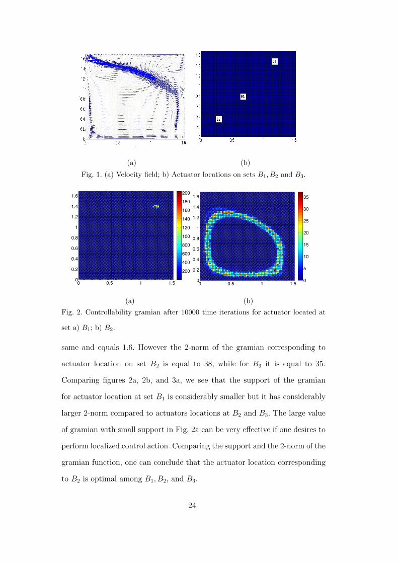
dimensional slice of the three dimensional velocity field as shown in Fig. 1a.
The dimensions of the room are as follows: 0 ≤ x ≤ 1.52m and 0 ≤ y ≤ 1.68m.
The order of magnitude for the velocity field is O(1). The Reynolds number
of the flow is Re = 76725 and the Prandtl number Pr = 0.729. This makes
1PrRe
≈ O(10−5), and hence the zero diffusion constant assumption (Assump-
tion 4) made in this paper is justified. The Reynolds number for the flow rate
22
is in turbulent range. The k − ε model, which is Reynolds Average Navier-
Stokes (RANS) model [17] is used to obtain the velocity field as shown in Fig.
1. A commercial CFD software Fluent was used to solve the coupled set of
governing equations for pressure, temperature, turbulent kinetic energy, tur-
bulent dissipation and velocity. No slip boundary condition was applied at all
the walls.
For the purposes of computation, we employ set oriented numerical methods
for the approximation of P-F semigroup Pt [18]. We divide the state space into
finitely many square partitions denoted by {Di}Ni=1. The set Di’s are chosen
such that Di∩Dj = ∅ for i 6= j and X = ∪Ni=1Di. The finite dimensional matrix
approximation of the P-F operator is obtained using the following formula [18]:
[P ]ij =m(φδt(Di) ∩Dj)
m(Di)
where m is the Lebesgue measure and δt is the discretization time step and φt
is the solution of vector field shown in Fig. 1a. Using the adjoint property be-
tween the Koopman and P-F semigroup, the finite dimensional approximation
of the Koopman semigroup U can be obtained as a transpose of P , namely
U = P ′
The computation results for this section are obtained with actuators and sen-
sors located at three different sets B1, B2, and B3. The locations of these three
sets are shown in Fig. 1b.
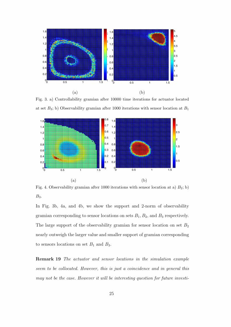
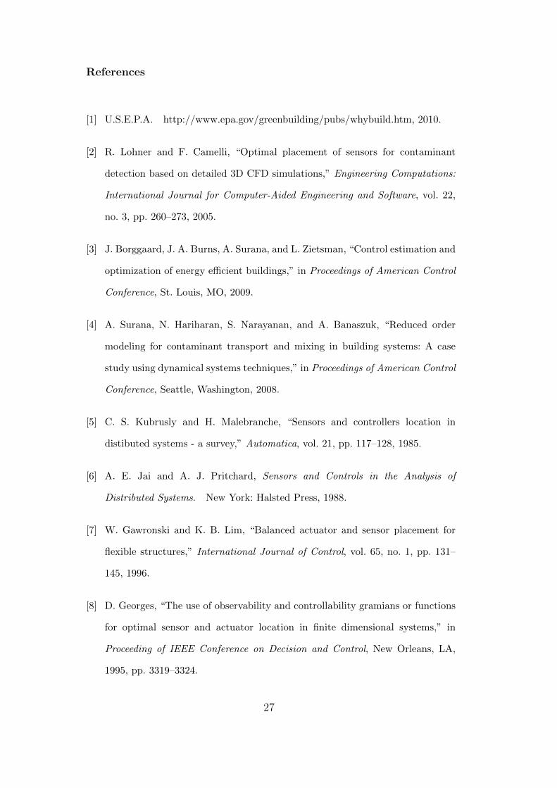
In Fig. 2b and Fig. 3a, we show the plots for the support of the controllability
gramian after 10000 time steps corresponding to two different locations of ac-
tuator sets B2 and B3 respectively. The support of the controllability gramian
corresponding to B2 and B3 locations of actuator sets is approximately the
23
(a) (b)
Fig. 1. (a) Velocity field; b) Actuator locations on sets B1, B2 and B3.
0 0.5 1 1.50
0.2
0.4
0.6
0.8
1
1.2
1.4
1.6
200
400
600
800
1000
1200
1400
1600
1800
2000
(a)
0 0.5 1 1.50
0.2
0.4
0.6
0.8
1
1.2
1.4
1.6
0
5
10
15
20
25
30
35
(b)
Fig. 2. Controllability gramian after 10000 time iterations for actuator located at
set a) B1; b) B2.
same and equals 1.6. However the 2-norm of the gramian corresponding to
actuator location on set B2 is equal to 38, while for B3 it is equal to 35.
Comparing figures 2a, 2b, and 3a, we see that the support of the gramian
for actuator location at set B1 is considerably smaller but it has considerably
larger 2-norm compared to actuators locations at B2 and B3. The large value
of gramian with small support in Fig. 2a can be very effective if one desires to
perform localized control action. Comparing the support and the 2-norm of the
gramian function, one can conclude that the actuator location corresponding
to B2 is optimal among B1, B2, and B3.
24
0 0.5 1 1.50
0.2
0.4
0.6
0.8
1
1.2
1.4
1.6
0
5
10
15
20
25
30
(a)
0 0.5 1 1.50
0.2
0.4
0.6
0.8
1
1.2
1.4
1.6
0.5
1
1.5
2
2.5
3
3.5
4
4.5
5
(b)
Fig. 3. a) Controllability gramian after 10000 time iterations for actuator located
at set B3; b) Observability gramian after 1000 iterations with sensor location at B1
0 0.5 1 1.50
0.2
0.4
0.6
0.8
1
1.2
1.4
1.6
0
0.1
0.2
0.3
0.4
0.5
0.6
0.7
0.8
(a)
0 0.5 1 1.50
0.2
0.4
0.6
0.8
1
1.2
1.4
1.6
0.5
1
1.5
2
2.5
3
(b)
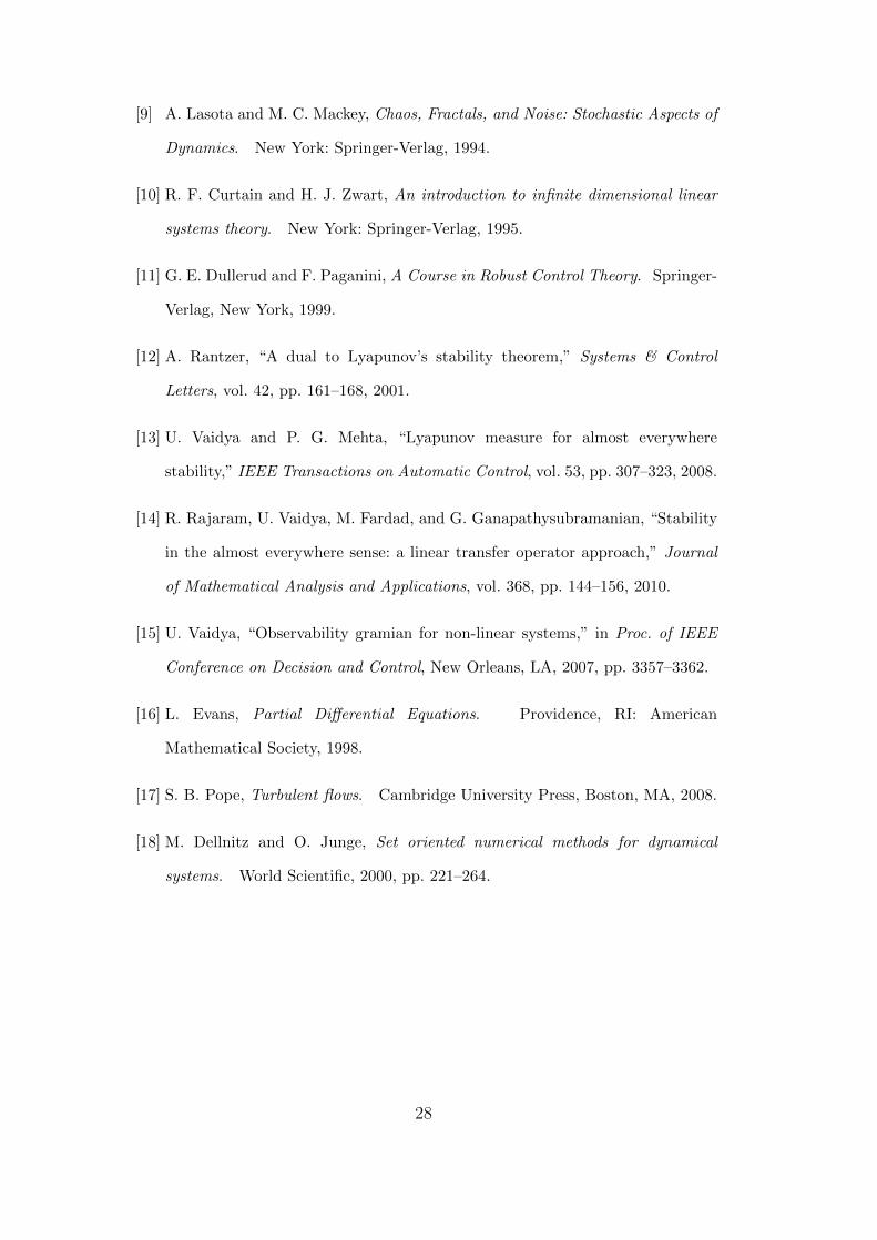
Fig. 4. Observability gramian after 1000 iterations with sensor location at a) B2; b)
B3.
In Fig. 3b, 4a, and 4b, we show the support and 2-norm of observability
gramian corresponding to sensor locations on sets B1, B2, and B3 respectively.
The large support of the observability gramian for sensor location on set B2
nearly outweigh the larger value and smaller support of gramian corresponding
to sensors locations on set B1 and B3.
Remark 19 The actuator and sensor locations in the simulation example
seem to be collocated. However, this is just a coincidence and in general this
may not be the case. However it will be interesting question for future investi-
25

gation. In particular, the combined problem of sensor and actuator placement
will be the topic of our future investigation.
6 Conclusion
In this paper, controllability and observability gramian based test criteria
are used to decide the suitability of given actuator and sensor locations. As
compared to purely computational based methods currently existing in the lit-
erature, our proposed approach provides a systematic and insightful method
for deciding the location of actuators and sensors in building systems. In par-
ticular, stability properties of the advection vector field are shown to play an
important role in deciding the location of actuators and sensors. In our future
research work, the explicit formula for the gramians will be exploited to pro-
vide a systematic algorithm for determining the optimal location of sensors
and actuators. Furthermore some of the assumptions made in the derivation
of control equations will be removed by incorporating elements of complex
physics involved in building systems.
7 Acknowledgement
The authors would like to thank Prof. Baskar Ganapathysubramanian for
providing data for the fluid flow vector field. Financial support of National
Science Foundation Grant CMMI-0807666 is greatly acknowledged.
26
References
[1] U.S.E.P.A. http://www.epa.gov/greenbuilding/pubs/whybuild.htm, 2010.
[2] R. Lohner and F. Camelli, “Optimal placement of sensors for contaminant
detection based on detailed 3D CFD simulations,” Engineering Computations:
International Journal for Computer-Aided Engineering and Software, vol. 22,
no. 3, pp. 260–273, 2005.
[3] J. Borggaard, J. A. Burns, A. Surana, and L. Zietsman, “Control estimation and
optimization of energy efficient buildings,” in Proceedings of American Control
Conference, St. Louis, MO, 2009.
[4] A. Surana, N. Hariharan, S. Narayanan, and A. Banaszuk, “Reduced order
modeling for contaminant transport and mixing in building systems: A case
study using dynamical systems techniques,” in Proceedings of American Control
Conference, Seattle, Washington, 2008.
[5] C. S. Kubrusly and H. Malebranche, “Sensors and controllers location in
distibuted systems - a survey,” Automatica, vol. 21, pp. 117–128, 1985.
[6] A. E. Jai and A. J. Pritchard, Sensors and Controls in the Analysis of
Distributed Systems. New York: Halsted Press, 1988.
[7] W. Gawronski and K. B. Lim, “Balanced actuator and sensor placement for
flexible structures,” International Journal of Control, vol. 65, no. 1, pp. 131–
145, 1996.
[8] D. Georges, “The use of observability and controllability gramians or functions
for optimal sensor and actuator location in finite dimensional systems,” in
Proceeding of IEEE Conference on Decision and Control, New Orleans, LA,
1995, pp. 3319–3324.
27
[9] A. Lasota and M. C. Mackey, Chaos, Fractals, and Noise: Stochastic Aspects of
Dynamics. New York: Springer-Verlag, 1994.
[10] R. F. Curtain and H. J. Zwart, An introduction to infinite dimensional linear
systems theory. New York: Springer-Verlag, 1995.
[11] G. E. Dullerud and F. Paganini, A Course in Robust Control Theory. Springer-
Verlag, New York, 1999.
[12] A. Rantzer, “A dual to Lyapunov’s stability theorem,” Systems & Control
Letters, vol. 42, pp. 161–168, 2001.
[13] U. Vaidya and P. G. Mehta, “Lyapunov measure for almost everywhere
stability,” IEEE Transactions on Automatic Control, vol. 53, pp. 307–323, 2008.
[14] R. Rajaram, U. Vaidya, M. Fardad, and G. Ganapathysubramanian, “Stability
in the almost everywhere sense: a linear transfer operator approach,” Journal
of Mathematical Analysis and Applications, vol. 368, pp. 144–156, 2010.
[15] U. Vaidya, “Observability gramian for non-linear systems,” in Proc. of IEEE
Conference on Decision and Control, New Orleans, LA, 2007, pp. 3357–3362.
[16] L. Evans, Partial Differential Equations. Providence, RI: American
Mathematical Society, 1998.
[17] S. B. Pope, Turbulent flows. Cambridge University Press, Boston, MA, 2008.
[18] M. Dellnitz and O. Junge, Set oriented numerical methods for dynamical
systems. World Scientific, 2000, pp. 221–264.
28