ad-a028 055 determination of seismic source depths …

II lUUftlllll^lJII ^^.pwnp^^«^^ inumm i ■ *■ ^^mippnvmm |MWMM<V«Wi.i|iaiipq9aTCH^P'flp«

/" A

U.S. DEPARTMEN1 OF COMMERCE

National Technical Information Service

AD-A028 055

DETERMINATION OF SEISMIC SOURCE

DEPTHS FROM DIFFERENTIAL TRAVEL TIMES

ENSCOy INCORPORATED

PREPARED FOR

AIR FORCE TECHNICAL APPLICATIONS CENTER

30 JUNE 1975

■--•-- . - - ■ - — _ - - .. .. . mt^m^mJ^^ .

^^-^

4

I

^

aM 6

225223

CO O 00 w o

REPRODUCCD BY

NATIONAL TECHNICAL INFORMATION SERVICE

U.S. DEPARTMENT OF COMMERCE SPRINGFIELD. VA. 22161

APPROVH) FOR PUBLT REIEASE. wsmtuTioN uNUAamax

E^SCO.IIVSC. Information & System Sciences Division

8001 Forbes Place Springfield. Virginia 22151

Pfione: (703) 569-9000

i ■npuipia*« »^■pwwtw^ww ■^^■^^P^WK-i i BIIIm i Hw*u i. ivw*iiii^«nMmw^P-<^v^« ■i- ■' ■ ™^gpwF

;

I« April I97J

DEPARTMENT OP DEFENSE FORMS

F-200.H73 DD Form im: Report Documentation Page

P234.7

tffCu'iiv ci*«k<ric »iitjM or «MM »«nf «*««

REPORT DOCUMr.HTATIUM PACE i. M»0«>f MUM»! m I frOVT ACCIkllO«! hb

• TITL« fvt« fv*iiir»;

DeterminntLon of Seismic Sourc Depths from Differential Tra- vel Times i. AuiMbRrt;

Edward Page, Robert Baunan

I PiarouMtMCC-nCAHi; *iio** H *-it *Mb *Dt/^iii

ENSCO, INC. 8001 Forbes PI., Spfld. Va

II. COMTHOLkIMC 0'riCC MAUC *«D ADCALIS

DCASD. Baltimore

VELA SeisnolO| ..1 Center 312 Montgomerv Street Alexandria, Virginia ZZ/iU (ft. Di|T*lijT,ONl1*Tt-tNT(t/,M, HlfMIl

» ■ICl»'ieMf»t»T*LO&MLm»Ei

»• TT^C OF Btro*)* • »IMtOD COVCAfD

£ Final Report

N/A

F08606-75-C-002S

13 •'•'JC»*«* fk tMfMT.faojCCT. T*m

1> HCFORT CAT!

30 .hinc 197.S I». NUMtCF •« ««Qlt

)» tCCUf>tTT CLASS f*/Ci«

»CnlOjLt

APPROVEn FOR PUBLIC RELEASE DISTRIBUTION UNLIMITED

tT. DliTM>lu1lOMlTAT|HCNTf*lt. • •«•»•<( m-\9f*4 in #J*<* ;:. if grflllll fr«w Fa<->fr;

■I tU'FktMEMlAnv NOTfl

It KtT •OT J (k'orx'nw« «t r«*#r«a «<*• (( »«^ •••»r an* Hmutty ►» kiack wt^»>»j

Seismic depth, depth phase, echo detection

10. AtlTWACt fCfin*— ww f —«« »l<» If <in«««fT Üi !<—|fr »y BJSJ j^SSj

New analysis techniques, developed for the detection of seismic depth phases, have been applied to three seismic events. These techniques were shown to greatly enhance the analyst's ability to determine SMsmic source

DD,^;". 1473 .»mo o o..0..„ PKICU SUBJtCT TO CHÄNGE MCunitv cc*in»ic*Ttoii o* Tnit ***.« ,»*•* r#r. «Mt«««

P-Ä00.1473

\UMKD SERVICES PROCimBStENT REGULATION

L f

_^ ,

II «w> I ■■ ^^immmmmm^- ' ' • ■ "■ " >I.I<«.FWI.>.. «■ > <. ... « .■>..■ _.,,,......

.. j»CCESS;i);j_(.r

KTIS DEC

IMWIOBMEO JUSll.'ICAIIO .

Ml Sect I □

D

tl

»itTRIBÜTIfl« '. f CODEI

DETERMINATION OF SEISMIC SOURCE DEPTHS

FROM DIFFERENTIAL TRAVEL TIMES

FINAL REPORT

Edward A. Page

Robert W. Baunan

July 1975

Sponsored by:

Advanced Research Project Agency

ARPA Order No. 1620

r

D D C

AUC 6 1976

JECdEITD B

APPROVED FOR PUBLIC RELEASE.

DISTRIBUTION UNLIMITED.

- — - ■ — ..- .._ -■,.. ——

^^~^~^^^^^^mmi^^m*~~~~ ■ i

;.

.

..

Notice of Disclaimer

:. The views and conclusions contained in this document are those of the author and should not be interpreted as necessarily representing the official policies, either expressed or implied, of the Advanced Research Projects Agency, the Air Force Technical Applications Center, or the U. S. government.

:.

:

) <

j

,^15» i I«P.B«II i imimrmn

i.

:.

SUBJECT: Determination of Seismic Source Depths from Differential Travel Times

AfTAC Project No - ..vnLA T/C71n

ARPA Order No-- -2551

ARPA Program Code No 5P10

Name of Contractor--- ENSC0) m

Contract Number F0806-75-C-0025

Effective Date of Contract i NoVember l9n

Report Period--- Novembcr ^ 1975

to June 30, 1975

Amount of Contract--- 549 *•«

Contract Expiration Date 30 june 1975

Project Scientist - Edward page

(703) 569-9000

c

—

m*^i^^mm^m~-

i

i

n :.

TABLE 0I; CONTENTS

1.0 INTRODUCTION

2.0 DEPTH PHASE ANALYSIS TECHNIQUES

2.1 Statistical Techniques for Utilizing Depth Phase Information Contained in the Seismic Coda

2.2 The Cepstrum Matched Filter Technique

2.3 Use of Seismic Travel Times to Account for Depth Phase Delay Time Variations along the Coda

3.0 APPLICATION OF THE NEW DEPTH PHASE DETECTION TECHNIQUES T0 THREE SEISMIC EVENTS

4.0 CONCLUSION

Pa ge

1- ■1

2- ■1

2- ■2

2- 6

2- 12

3-1

3.1 Analysis of the Illinois Event 3-1

3.1.1 Evidence of Improved Depth Phase 3-1 Detectahility Using Seismic Coda

3.1.2 Effect of Later Portion of Seismic 3-7 Coda on Detection

3.1.5 Cepstrum Matched Filter Interpretation 3-0 of Results

3.2 Analyses of the Kamchatka Event . --

3.3 Analysis of the China Event 3.J4

4-1

Appendix A Stochastic Cepstrum Stacking Appendix | Stochastic Cepstrum Pnasor Stack Appendix C Calculation of the Stochastic Cepstrum Stack and

Stochastic Cepstrum Phaser Stack Appendix D Synthetic Scismograms

1^

■ ■

■ ' "ii,in i MII nwr^^^^pjOTW

4.

D

i;

1.0 INTRODUCTION

The objective of this research effort was to further

investigate the applicability of statistical signal processing

techniques developed during the previous contract (Contract I

F0860b-74-C-0020) for the purpose of enhancing seismic source

depth determinations. These techniques were designed to improve

the detection and interpretation of seismic depth phase information

contained throughout the seismogiam. Three seismic events were

analyzed during this contract period, and the results obtained

clearly demonstrated the ability of these new depth phase detec-

tion techniques to obtain seismic source depths for events in

which conventional analysis was ineffective.

The primary interest in improving seismic depth phase detec-

tion is that depth phase information gives reliable estimates

of seismic source depths. Source depth is a critical factor in

the discrimination between man-made events and natu-al seismic

events since the maximum depth of burial for man-made events

is of the order of ten kilometers and earthquakes can originate

at much greater depths

At present, depth phase detection is performed by analyzing

the first arrival portion of the seismogram for the presence

of the pP and sP arrivals. Analysis is usually done through

attempts to visually identify the pP and sP first movements

from seismograms recorded over a suite of stations. Identifica-

tion of the depth phase is verified when the variations in the

differential travel times are in agreement with the differential

travel time tables for the given source to station differences.

Correlation techniques are also applied to first arrival

1-1

V

- ■- ■ -

. i-UiUlii i i i mmnuu, i

i.

portions if seismograms in an effort to detect the presence

of the depth phases and their delay times. Both of these

detection methods use only the first arrival portion of the

seismogram containing the p? and sP first movements and ignore

the abundance of depth phase information contained in the direct

and surface reflected waveforms present throughout the entire

seismogram. Ignoring this additional depth information limits

the inherent detectability of these methods.

Our efforts have focused on the development of a cepstral

estimation procedure which makes constructive use of the depth

phase information present throughout the seismograms recorded

over a suite of stations. This analysis is based on techniques

which account for the depth phase delay time variations asso-

ciated with the later seismic arrivals and on a technique which

utilizes the phase differences between the direct and surface

reflected arrivals in order to enhance the detection of depth

phases. A Cepstrum Matched Filter technique was developed to

aid in interpreting the typically complicated cepstral patterns

resulting from this analysis. It has proven to be very valuable

i: further improving seismic depth phase detection.

Based on the work done to date, all indications are that

these new seismic depth phase detection techniques will greatly

enhance the analyst's ability to determine seismic source depths.

1-2

IMMMIHIIMtaälll

mmm i niiBiiiiiiüipiiMmvpiw^nn« ■ «■■■•. ■ .—.-. —•■. — Mj^ .,-. . .1 , i f i mm —— ■ '—" ■

• .

2.0 DEPTH PHASE ANALYSIS TECHNIQUES

The most accurate estimates of teleseismic source depths

are obtained throunh the measurement of the differential travel

times between the direct seismic arrival (P wave) and the

surface reflected arrivals (pP and sP). The pP phase follows the

P phase by roughly 1/4 second for each kilometer of source

depth, and the sP phase follows the P phase by about 1/3 second

per kilometer of depth. Therefore, by obtaining estimates

of P-pP or P-sP delay times to within 1/3 second, it is

possible to estimate the source depth to within one or two

kilometers. Depth estimates of this accuracy are extremely

useful in distinguishing natural events from man-made events.

The present difficulty in using depth phase information to deter-

mine source depths is that the depth phases are identified for

only about half the events analyzed using the conventional techniques .

Depth phase detection is generally performed by visual

identification of the P. pP, and sP first movements (See Figure

1). Identifications of the depth phases are verified when the

variations in the differential travel times are in agreement

with the differential travel time tables for the given source

to station distances. Both the detectability and accuracy of

these delay time estimates are limited in this procedure since

both are based on identifying the P, pP, or sP first movements.

Correlation techniques are sometimes used to analyze the first

arrival portion of the seismogram (that portion containing the

P, pP, and sP first arrivals) for the presence of the pP and

sP phases. However, both of these detection techniques have

limited detectability and resolution since they use depth

2-1

- - - -

—»"—--"- -1- —

1 sP

1 1 EtatlonAzimuth DUt.(kn>)

CP-CL 132.5° 7760

I MN-NV 132.5" 8)20

4k^ i

I HI-NV 133.6 8500

MAAV^^V^^V»^ ^V^..,». ^../.jiftA^A-ife KN-UT 136.3 737 5

\it»^vVL*<i^/"^'-/'tA -•'«•■»'V

U1

HL-ID 136.5 8490

W^i P*^ W^ftf "^1 f^Y^'■i'A^L*^)' * W » ->I,-^L " ' ' ' / 1 "

FS-AZ 137.0" 7625

\ l DR-CO l40.oO 7615

'»'■"'X/'v^w-w-i * Z'' * A^ 'W»«-«»v PM-wy 143.5° 7815

WN-SD 148.6 77 65

.

0

-A k-. 0 sec.

Figure 1. An Example of Unfiltered Z-Component

Seismograms showing Initial Phases

(Bolivia Event 12:02:22 Z 19 July 1962).

2-2

■■-1 'i ii „M^^mmtm

H"M ' ■'!■ ' W» ■- M

i. i.

phase information contained only in the first arrival portion

of the seismogram and ignore the abundance of depth phase

information contained in the direct and surface reflected

waveforms present throughout the rest of the seismogram.

In the following section, we discuss statistical techniques

for utilizing depth phase information contained in the entire

seismogram. These techniques are Stochastic Cepstrum Stacking

and Stochastic Cesptrum Phaser Stacking.

2-3

--- ■■-■ - - ■-•■■■ - -■ ■

_. . .... .. ^

.

2.1 Statistical Techniques for Utilizing Depth Phase

Information Contained in the Coda

In order to constructively use the depth phase information

contained in the seismic coda, one must he aware of variations

in the depth phase delay times ohserved along the coda. The

largest of these variations originate from the differential

travel times between later seismic arrivals such as PP, PcP,

PPP, etc and their associated surface reflections pPP, sPP,

pPcP, sPcP, pPPP, sPFP, etc. Other contributions to the delay

time variations include background noise, multipath effects, and

differential distortions in the seismic waveforms caused by the

properties of the medium. A cepstrum estimatu , procedure

that allows for these delay cime variations has proven to

be very useful. As described in Appendix A, "Stochastic Cepstrum

Stacking," this procedure allows for these delay time variations

by stochastically averaging cepstra calculated from different

portions of the seismogram to enable improved detection of pP-P

time delays. With conventional averaging of these cepstra, detec

tability is significantly reduced.

In many cases, further enhancement in depth phase detecta-

bility is achieved by utilizing the relative phase difference

between the direct and surface reflected seismic arrivals. In

Appendix B, "Stochastic Cepstrum Phaser Stack," we show that

the phase of the cosinusoidal modulation of the power spectrum

resulting from the presence of the delayed surface reflected

arrival can be assigned to each cepstrum amplitude and these

values can then be treated as cepstrum phasors. These phase

angles can be used to help distinguish cepstrum peaks resulting

from surface reflected arrivals from those resulting from spu-

rious sources.

2-4

;

ü Both the Stochastic Cepstrum Stack and Stochastic Cepstrum

Phasor Stack techniques were used in the analysis of events

during this contract. The results are given in Section 3. The

detailed mat lematical description of the steps involved in com-

puting these cepstra is described in Appendix C.

In the next section, we discuss a Cepstrum Matched Filter

technique which was developed as an aid to interpretating the

deptli phi?se information contained in these computed cepstra.

2-5

■ Mk-UiMMMMdMMta ■ —- ■" ^^^^^HMiM^^^M^*^^ ^

..

.

■

2.2 Cepstrum Matched Filter Technique

\

The previous sections described techniques which enable

one to utilize the depth phase information contained in the

seism- coda and thereby enhance the appearance of the cepstrum

peak corresponding to the pP-P delay time. If one can identify

such a cepstrum peak, the source depth can then be accurately '

determined from differential travel time tables, provided the

velocity versus depth assumptions are valid. However, ceostrum

peaks corresponding to the pP-P time delay tj. the sP-P time

delay tj, as well as the sP-pP time delay, will in general result

from a single seismic source. According th the particular cepstrum

algorithm used, additional peaks will appear at nx^mr, (where

n and m are integers) when non-linear operations are included in

the cepstrum computation. Thus, there is in general a complicated

set of cepstial peaks corresponding to a single source depth.

In thif section, we describe the Cepstrum Matched Filter (CMF)

technique, which is an automatic method of recognizing the presence

of a cepstrum pattern corresponding to a particular source depth

over a range of possible source depths.

If one assumes that the cepstral peaks appearing at the

PP-P. sP-P and sP-pP time delays dominate the expected cepstrum

pattern for an event, then one can formulate the CMF algorithm

I« the fo:lowing way. Consider the cepstrum to cons-st of N

amplitude values CP(n) for the time delays tn=Cn-l).At, where

n 1.2,3...M. Then the synthetic cepstrum (CS) expected for an

event at a given depth and distance corresponding to a pP-P delay time of T, can be represented by:

2-6

..

.

[j

i.

CSCn.T.ci) = QCn,(a-l)T) + Q(n,T) + QCn.at)

with a= Tsp-p/Tpp.p> and is the ratio of delay times for sP-P

and pP-P. Also Q is defined by

Q(n,T) = 1 ; if T-At<t <T+At ,

= 0 ; otherwise .

Thus, CS is represented by three unit amplitude peaks located at

the sP-pP, pP-P, and sP-P delay times, each peak consisting of

three adjacent delay time points.

The CMP output at time delay t is defined '.o be the maximum

zero lag correlation of the computed cepstrum (CP) with the

synthesized cepstrum (CS) for a source depth having a pP-P delay

time T computed over a range of ratios n. This can be written as

CMF(T) Max I CPfnl-CSfn T «A if CPCT)>.7-CP(aT) „tjl l J L^n'T'an - and CP(T)>.7-CP((cx-l)r

= CP(T) ; otherwise

Here, o^ and a-, are set from the expected range of values

for a for a given range of possible depths. Values of a, = 1.25

and a2 = 1.55 were used for the event distances and depths encoun

tcred in this research. The constraints iimoscd require that the

amplitude ol the cepstrum peak at T must be at least 7 times

the amplitude of the cepstrum penks at both «T and («-I),

This eliminates detection of cepstral patterns for cases in

2-7

I

which the strength of the pP arrival is considerably less than

that of the sP arrival. Thus, a cepstrum peak at t resulting

from a pP arrival for an event will not contribute to the CMF

output for an apparent event having an expected sP-P delay time

of T, without the significant presence of a pP arrival for this

apparent event.

As an example of the application of this technique, consider

Figure 2. At the top of the figure is the cepstrum calculated

from an event of known depth having both the pP and sP depth

phases clearly identifiable. This cepstrum pattern is dominated

by three peaks corresponding to the sP-pP, pP-P, and sP-P delay

times. Upon interpreting this cepstrum for an unknown event depth,

one sees that each of the three peaks has the possibility of

corresponding to the pP phase. The CMF output is plotted at the

bottom of Figure 2 and indicates a much stronger emp'iasis on the

peak corresponding to the correct pP-P delay time fcr this event.

This result reflects the fact that this cepstrum pattern primarily

consisting of three peaks is' in strong agreement with the pattern

expected for a single event having this pP-P delay time. The

lesser probability that the relative location of these three peaks

was coincidental, and that one of the other two peaks actually

corresponded to the correct pP-P delay time, is indicated by the

presence of CMF output peaks at those delay times having reduced

amplitudes.

Another example of the usefulness of the CMF is shown in

Figure 3. At the top of this figure is a cepstrum calculated for

the same event, but using data recorded at a single station.

The figure contains four cepstrum peaks having approximately equal

amplitudes making the interpretation of the source depth diffi-

cult. At the bottom of the figure is the CMF interpretation of

this cepstrum which reveals a strong emphasis on the peak

2-8

MBBMBk—jaitMM

i. i.

C EI'ST RUM

CEPSTRUM MATCIini)

FILTER OUTPUT

tine delay

(seconds)

amplitude-

(sctunds)

Pigure 2. Ccpstruni and Cepstrua Matched Filter output computed fro« data recorded at tcvera] st.-it ions for an event with well defined depth phases

2-9

..Mi^amMB-M .

y

.

amplitude

CE^ÜTRUM

CBPSnm MATCHEd FILTER OUTPUT

time \ /| delay

amnli tudc

))V-V do lay time

P^T^T^^ Seconds) 8 •• M

1.1 tj — W -s) • C1 (4 — Cl •— <J *> «« -j i i/j

Figure 3, Cepstrtra and Cepstrtui Matched Filter output computed from data recorded at a sincle station for an event with wcl! defined deptli pliascs.

2-10

corresponding to the correct pp-r delay time. Additional examples

showing the usefulness of the CMF technique in determining seis-

mic source depths will be shown in Section S.

2-11

J

:

?.3 Use of Seismic Travel Times To Account For Depth

Phase Delay Time Variations Along The Coda

In the previous sections, we have discussed techniques which

statistically allow for the variations in the differential delay

times along the coda in order to enable more of the depth phase

information to contribute to the depth phase dete^Lion. However,

allowing for depth phase delay time variations through use of the

Stochastic Cepstrum Stacking technique proves to be useful up to

stochastic window widths of about 1 second. Events of interest

to this work can have delay time variations of several seconds;

for example (pP-P)-(pPP-PP) = 3.9 seconds for a depth of 50

kilometers and an epicentral distance of 30°. The stochastic

stacking technique could not encompass such variations without

a severe loss in detectability and resolution, unless that

portion of the coda containing the PP arrivals from the analysis

is eliminated or some means is utilized to normalize this data

to the direct phase. t

In Figure 4, we show an illustration of 5uch a case. Here,

seismograms are depicted for recoidings of an event at two sta-

tions. From the illustration, we sQe that the pP-P delay time

is considerably larger than the pPP-PP delay time, and, tnere-

fore, the cepstrum peaks cjmputed from samples 1 and 2 will

not constructively average. The right side of Figure 4 illus-

trates that the peaks in the CMF output would also lie at differ-

ent delay times and can not be constructively averaged in a

linear sense. A similar situation is found with the data recorded

at station 2, but here the delay times are, in addition, altered

relative to station 1 by the station moveout. *0ne would like to

be able to combine the CMF outputs computed from the four samples

in a manner which would allow these peaks to constructively rein-

force at the pP-P delay time. This is shown at the bottom of the figure.

2-12

.

Station 1 DP SP PP pPP sPP

IÂAJ. l{^l\jüw\J\fv^ Mbk ■aaple 1 {- snmp]c 2 i

Station 2 /

tA&fJuîJHA** jyutoh LyÂ+KA*

sample 1

sample 2

sample 3

sample 4

CEPSTRUN MATCHED FILT iR OUTPUT

i

• i time delay

K-WAKAWUA ̂AA^^v'^^/

I

V>J[[AÂ A^«

Contained Cepttrua Matched Filter output» compensated for : j|

1. depth phase delay time differences of later phases.

2. station moveout

Figure 4

KM .'^/v'v.'W'-' wA.v«v^^

j time delay I

^^w^Wv, -Â^w

i

'VW 4^^

depth

2-13

maiiir an i ir ^laamtinin -— ■ --if i i -*—-^—~.^—. ...-■^... ..■- ,...

i.

.

If one calculates the delay time variaMons expected

along the coda for various event depths and distances using

a seismic arrival time program, the appropriate delay time

corrections could be applied to the CMF output of each sample

before averaging. The degree to which the CMF output peaks

slacked would then be a measure of how well the various depth

phase delay times, computed along the coda and at different

stations, all agreed with a given source depth assumption.

Using such a procedure, all of the depth phase information

contained in the seismogram would contribute to the depth phase letect ion.

In order to develop such a procedure one first needs the

appropriate travel time information. Differential travel times

such as sP-P, pPP-PP, sPP-PP. pPcP-PcP, sPcP-PcP, pPPP-PPP, and

sPPP-PPP are not easily obtained from existing tabulations.

These are the phases which comprise that portion of the seismic

coda usually available for depth phase analysis. To determine

these travel times, a ray tracing program based on the spherically

symmetric Isotropie earth velocity model used to calculate the

BSSA (Bull.Seism. Soc. Amer., Vol. 58, No. 4(extract), August

1968) seismological tables for P phases was used . The program

was checked by exactly reproducing selected travel times listed

in the BSSA tables.

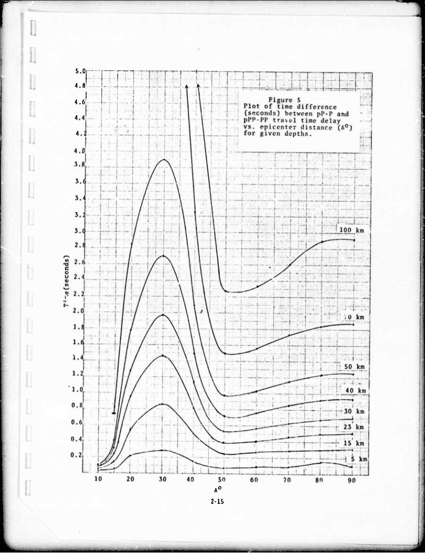
Figures 5, 6, and 7 give the computed time differences for

the (pP-P)-(pPP-PP), (pP-P)-(pPPP-PPP), and (pPcP-PcP) - (pl'-P)

time delay differences. These charts give the expected shift

of the CMF output peaks relative to the pP-P delay time, com-

puted from portions of the coda containing either the PP, PPP,

or PcP arrivals. One notes that these shifts are more signifi-

cant for event depths greater than % 10 km. Through use of

these charts, cepstra or CMF outputs computed from different

2-14

■ -■ ,

r

i.

s.

4.8

Or-- m i T-rr:: rr -i • - ;

2-15

i. i.

!

T"-

Figure 6 Plot of time difference (seconds) between pP-P a pPPl'-PPP travel time del vs. epicenter distance ( for given depths.

IPS ml

A6) i : ; i

1 : ! • : i

. i J ■

—1. ._ ..

! j. ■

\

A" ■ - ;

:.': V . ... > L

' .; I :\

■ ■ ■

-'-■■-

...i '.[X "":

10° 20 30° . i J i -L-L.-L 1

.10° | l . r-r-r

40° 60° 70° A0

2-16

80° 90l

I T

I

I.

Ü m*

70 km i :,

Z'.t.: i ......

T:J:i:

mm Figure 7

Plot of time difference (seconds) between pPcP-PcP and pP-P travel time delays vs. epicenter distance (A

0)

for given depths

- - „ .,. ,.,.,. ., .m^m^^tt^

r ■•■ ^mmm^m^m^^^^^m <^m-^mmnmm

portions of the seismogram can be constructively averaged to

produce a prominent peak at the pP-F delay time. Such a tech-

nique should prove very useful in improving hoth depth phase

detection and depth phase delay time resolution.

The travel time differences for pPP-PP, pPcP-PcP, and

pPPP-PPP are shown in Figures 8 and 9. In Figures 10 and 11

are shown plots of the pP-P delay times for the depths 5 to

40 km and 5 to 100 km respectively. In Figure 12, the PP-P,

PcP-P, and PPP-P delay times for a range of depths and distances

are given. The travel time differences plotted in Figure 12

can be represented by single curves for source depths between

5 and 100 km since the depth dependence turns out to be very

weak. This points out that these phases alone are not useful

for depth determination. The arrows in the figure indicate

the minimum epicenter distance to which the PP, PPP, and PcP

phase exists for given depths.

2-18

u.

^■~ "

[i

.

- --- - ■ "-

^mmfrnt^^^^mmm mi*'^^*^m*^**mm ■^■P"^^^«^^ » ■«*—*»

1. i; i.

;

22

20

TT

.,. ...

i:

| :

.J__1.U

Figure 9 Plot of travel time difference for pPPP-PPP vs. depth (km) for given epicenter

....

^ -.;■

I ~l " ■[. '"I—1—

: ■':•] ;

-t 1 r

,' 80o-90o

20 30 40 50

Depth(km)

60 7 0 80 yo

. .

..

***mmi^mm*~mm^*r

'..

I.

I

1

12 B^;:

lip 11

10

TJL-

:l: :.

rAlr.'ii " ;;: 1 ..:;.:.

Figure 10 1 Plot of travel time differ

once (seconds) for pP-P I vs. depth (km) for given

epicenter distances (A0)

i::.

•a c o u

in o

V E

TVi

10 is 20 25 Depth(km)

2-21

30 ss 40

.. _ ■ - ■ ■

.-^Ä""

- —

- ■■—■■ •***imm^m**r^mimm mPTHM^NP^^

—

..

3.0 APPLICATION OF THE NEW DEPTH PHASE DETECTION

TECHNIQUES TO THREE SEISMIC EVENTS

Three seismic events, having known source depths, were

chosen for analysis using the new depth phase detection tech-

niques. These events had depths of 24, 178,and 53 kilometers

and represent a range of signal to noise ratios such that

visual identification of the depth phase is easy for one event,

difficult for another and impossible for the third event.

3.1 Analysis of the Illinois Event

The Illinois Event of 11/9/68 was analyzed for differential

travel time information using data recorded at six LRSM stations

(KN-UT, MN-NV, PGZBC, WHZYK; FB-AK, NP-NT) at a 20 pts/sec.

sample rate. This event was selected because the pP phase can

be accurately identified from the seismograms (see Figure 13)

and results obtained using f lie new techniques could be verified.

3.1.1 Evidence of Improved Depth Phase Detectahility Using

Seismic Coda

The analysis was carried out by first computing cepstrums

using 14 consecutive 12.8 second data samples from each of the

seismograms. (The same analysis was carried out using samples

which overlapped by 250o and SOI and no significant changes

in the results were noted.) Cepstrum phasori as well as the

cepstrum amplitudes were computed using the steps described

in Appendix C. In Figure 14 are plotted the cepstrum stacks

3-1

i:

--■

/

tC

<

;«.

r

<i

-r

,?

^

I

u o

JL

>

4! i >

5: >

?

>.

■ >

T

1

?

:>

$;

^> \

P

^1

cz:

U3 »— o

I M ••H u.

H^N r""* U^ u: r- u:^-< H^ PO '•. o «o >-o <o XO

I Ol i •• 1 11-- 11 o ■ r l l o X. •■« B <-j O'l X. '-"I fO «t Oi -r us^ >:^ (X^ ^; v—' U. krf kw

3-2

,l ■-^"»•^•l ■ i ■■ """""^"^Wl

14a

14b

14c

14d

CEPSTRUM STACK

(1ST - 12.8 SECOND SAMPLt

FROM EACH STATION)

CEPSTRUM STACK

(5 - 12.8 SECOND SAMPLES

FROM EACH STATION)

CLPSTRL'n PHASOR STACK


FROM EACH STATION)

SYfiiiinic ripsmn STACK

(TJ - 7.0i T2 - 10.0)

r,'il"i"lr"r"i'"il"i"li^»

-1—r—1—1—1 i.^

pF-P

sP-pP

sP-P

*\t tire delav

^—> (sec)

Figure 14. CEPSTRUM STACK FOR ILLINOIS EVENT

3-3

. ■ - -■

,

■wm« wwpwnPimpHv«^^^ w^mm^*rymm*r**mmi*mmmmm ^a^i^mpimi mm mn

computed by averaging six cepstra calculated using the first

12.8 second data sample from each station (the start of these

data samples was \ 1 second before the onset of the P-wave).

There is a dominant peak at ^6.8 second delay time corresponding

to a pP-P delay time for a 24 km deep event recorded at approx-

imately 30°. In Figures i4b and 14c, are the cepstrum stack

and cepstrum phasor stack each calculated by averaging 30

cepstra computed using the first five 12.8 second samples from

all six stations.

:

In both of these cepstrum stacks, a clear peak at ^9.8 seconds

has now emerged and corresponds to the known sP-P delay time

for this event. This is evidence that improved depth phase

detectability is obtainable by including data from the seismic

coda in the analysis. Figure 14d is a plot of a cepstrum stack

computed from data simulated to have pP-P and sP-P delay times

of 7 and 10 seconds respectively. There is good agreement of

this theoretical cepstrum result with those computed from the

data. (Appendix D describes the steps used to generate the

simulated seismogram.) Figure 15 shows the cepstra calculated

for the individual stations used to record the Illinois Event.

Additional evidence that the coda contains usable depth

phase information is obtained by analyzing a portion of the

coda starting at 12.8 seconds from the onset of the P-wave.

By eliminating the first 12,8 seconds of the seismogram and

averaging five 12.8 second samples from each station, one still

achieves clear detection of both the pP and sP depth phases

as is shown in Figure 16.

3-4

^ ...

ww^^^^mmrmm ^^mmmmw^m**r*^^~**^^*'*~'^^~** m i ■■ " ■" " n^-mm^mmm*

:.

USE OF SEISMIC CODA IN DEPTH PHASE DETECTION

CEPSTRUli STACK


FROM EACH STATION)

CEPSTRUH STACK

(5 - 12,8 SECOI.'D SAfiPLCS FRO« EACH STATION

. STARTll.'G AT 12.8 SECONDS

FROM FIRST ARRIVAL)

delay time (sec)

|IH|iiqmti.Mpt,1,„|„l,t,|,<,„t,,,1,,,p,,)„ w

delay time (sec)

C Ut Ot -Nl d fO UJ '1 - 10

•- Cl J* tr 1. (ri «! CJ B ft ir " K V» I til t.) C) 4- ir ^ *j, Kti

Figure 16. Copstrums computed with 'ind without the first

arrival portion oi the seismojjram included.

3 -6

mmm

1 '^^" ■ »laiimn^i ijii.iiiL HPIHRI«^«9^MffM MHIII II ■■■. IIPH ^■PPWIWiWW»

.

3.1.2 Effect of Later Portions of the Coda on Detection

From the results presented in Figures 14 and 16, it is

clear that depth phase information contained in the first minute

of coda can be utilized to impro e depth phase detection. How-

ever, by including the next 90 seconds of data in the analysis,

detection is found to deteriorate because the differential

delay times are substantially different in this portion of the

coda. As was discussed in Section 2.3, one must deterministically

account for the delay time variations associated with the later

seismic arrivals when these variations are greater than % 1 second.

The results of using different portions of the coda for the analy-

sis are shown in Figure 17. In Figure 17b is the cepstrum resulting

from an analysis which included the first 3 minutes of the seis-

mograms. This cepstrum does not have clearly defined peaks and is

essentially the result of combining the cepstra calculated from the

first minute of data (Figure 17a) with those calculated from the

next 90 seconds of data (Figure 17c), the latter having dominant

peaks at 4.9 and 7.8 seconds. The 4.9 second delay time is in

agreement with the range of both the pPP-PP and pPPP-PPP delay

times for a 24 km event recorded over a 20° to 40° range (see

Figures 8 and 9.) From Figure 12 one notes that both the PP and

PPP phases are present in the second minute of the seismogram for this event.

Thus, if one were to anticipate these delay time shifts for

a given depth, one could then shift and average these cepstra such

that they would reinforce at the pP-P delay time. This procedure

would allow the depth phase information from more of the coda to

contribute to the detection and avoid the deterioration of results

3-7

..^ —^ ,— —--. ^— . M.mu , — .._ -

■ ■l-1 ■ ■ -— '■■ -wmmmmmam *^m

J>

ZDL

— hail

■ ■ V 1 o X ■ ■ t~

■ 1*1 Sei!

iiil s — u >

i.

z=4

'Zi

s %

«I

5^

i I«

u

w 2^ C M H Di O K CO 3 /—i o w 1—( p ct: S < o > u

w s: CO c Di z U- K-)

o >« M < H -3 3 W a. O ^. o W u s

t—1

ui H u V '

< H < V) Q

O

g u CC PJ E-< E CO F a, PJ u. u o

N

•H

litl 5 'a !

a J ► s

ili

ö I in

E i

3-8

. . .„.

■ I "■ ■'

occurring when the stochastic stacking window cannot absorh

these large delay time variations. For the Illinois event,

analysis must be restricted to the first 90 seconds of data if

one does not apply a delay time compensation according to travel

time information for the later phases.

3.1.3 Ccpstrum Matched Filter Interpretation of Resu1t

The results shown in Figures 14 and 16 indicate three

dominant cepstrum peaks corresponding to the sP-pP, pP-P,

sP-P delay times. In general it is difficult to determine the

source depth from this information since the relationship among

the peaks is not immediately apparent by visual inspection. An

interpretation of these results can be substantially improved

through use of the CMF technique discussed in Section 2.2.

Figure 18 shows the resulting CMF output plotted with a scismo-

gram recorded at KN-UT for the Illinois event. The CMF output

shows a single dominant peak corresponding to the pP-P delay time

for this event and is in agreement with the identification of the

pP-P delay time observed in the seismogram. This result reflects

the fact that all three cepstrum peaks arise from a single source

depth having pP-P delay time of \ 6.8 seconds, averaged over the

six stations. The CMF technique allows improved and automatic

determination of the source depth from the computed cepstra.

3-9

—»!■»■—T~—w .11 lllf^^^^^^w"

>.

■o g - o A- u r! •

<- 12. 12.8

2

cd

- 9.6 -

8.0

r 6.4

4.8

3.2

- 1.6

0.0

o

U 4-1

n o 3 >« ^. 4-" O W 4J

O H

9

5 'S s r M

0) to

u ra <-> to

o v, re .c

C. o

c o > w

O C

u ««

4)

i 3-10

-- ■■■— -■- ■ ■

3-2 Analysis of the Kamchatka Event

The Kamchatka event of 3/15/69 was next analyzed for the

depth phase delay time using data recorded at 20 rts/sec at

the four stations PIWY, RKON, DRCO, and LCNM. The first minute

of the seismogram for this event is plotted in Figure 19. Cep-

stra were computed using the first 102.4 seconds of data re-

corded at each station (additional coda data was not available

for this event). A stochastic cepstrum stack was then computed

using stochastic windows ranging from 0 to 3 seconds. At the

top of Figure 20 is plotted the stochastic cepstrum stack com-

puted using a stochastic window of 2 seconds which gives rise

to a significant improvement in detectability over conventional

averaging techniques. The stochastic window served the purpose

of allowing for delay time variations primarily associated with

station moveout which was as large as 1.5 seconds for these re-

cordings. In the anal/sis of the Illinois event the station

moveout gave rise to a maximum delay time difference of % .6

seconds and stochastic stacking gave an insignificant improve-

ment in detectability over normal averaging. At the top of

Figure 20, dominant peaks are observed at \ 14 seconds and at

*- 42 seconds. To interpret this cepstrum pattern, the CMF tech-

nique was applied and the resulting output is plotted at the

bottom of thi:. figure. One again observes additional emphasis

on the cepstral peak appearing at the correct pP-P time delay for

this event which indicates a source depth of % 178 km.

3-11

^ — . i

, ^__^„,— 1 ■ "■ n :.

o, «

OJ

U

■

3-12

J

mm ^mm^^mmm

B u o E u

•i-l o

P.

? 3

>

<

n »* W >• ••' •• j| % ■ v> <J ** t. CL»' •- »« »» w ^ n u >: i»- o

5-13

' p I

3.i Analysis of the China Event

The third seismic event analyzed for depth phase informa-

tion using the new techniques was the China Event of 6/5/64.

This event was analyzed using data recorded at 20 pts/sec at the

three stations GG-GR, BMO, and UGO. As is seen in Figure 21,

the recordings have very poor signal to noise ratios, and it is

impossihlc for an analyst to determine the depth phase delay

times visually. For this event, 9 cepstra were computed from

the first three consecutive 25.6 second samples for each of the

three stations. These cepstra were stochastically averaged using

a stochastic window width of % 1 second, and the stochastic cep-

strum stack was computed using hoth the cepstrum and ccpstrum

phasor techniques. The cepstrum phasor technique gave somewhat

better results in this case and is plotted at the top of Figure

22. Two cepstrum peaks stard out at W and ^ 14 seconds but

are not very convincing. However, by applying the CMF to this

data, a more distinct peak appears in the CMF output at the

correct pP-P delay time for' this event (Figure 22, bottom). This

peak appears at % 14 seconds and corresponds to an event depth

of ^ 53 km for these source to station distances. This result

gives a striking example of the ability of these new techniques

to detect the depth phase and obtain accurate source depth esti-

mates from recordings of events in which conventional analysis would fail.

3-14

•BMBMaMMiHai

I I. e

J

.-'"

4T.

of. ^> oo i en

I: s c.

„«*

J

a. jr

<1

■ o o o ::« (0 ■—-

<*,

? T u o

1

'J.

;t ---

i o O «o J--

4

NO

w

3-IS

..

■

E

^^

X) o U «J 4J 2 rt u >: ^ E o 3 ^ I- *-> O •/I «J

«si

O U

a.

3-16

4.0 CONCLUSION

During this research effort, new seismic depth detection

techniques have been investigated to determine whether they

could significantly enhance one's ability to obtain accurate

source depths at teleseismic distances. Three seismic events,

each having well established depths, were analyzed using these

techniques and clear detections of the correct pP-P delay times

were obtained in each case. For at least one of these events,

conventional depth phase analysis was not capable of obtaining

a source depth estimate using the data analyzed in this work.

Results of the research demonstrated that these new techniques

represent a major improvement over conventional depth phase

detection procedures through advances in both the detection and

interpretation of seismic depth phase information. The new

analysis method involved techniques which utilize more of the

seismic depth phase information contained in the seismogram

and techniques which also interpret the typically complicated

cepstrum patterns to extract source depth estimates.

These techniques could next be incorporated in a seismic

depth phase analysis package which would be of valuable assist-

ance to the analyst. Such a package would automatically analyze

the seismic data to extract accurate source depth estimates by

determining the degree to which the cepstrum patterns, computed

from different portions of the seismograms recorded over a suite

ot stations, agreed with those expected for a given event depth.

This analysis would automatically make constructive use of depth

phase information contained throughout the seismograms and should

give the analyst the ability to determine accurate source depth

estimates for a significantl> larger percentage of events then

is presently possible.

4-1

—_ — - - ■ ■ --

..

APPENDIX A

STOCHASTIC CbPSTRUM STACKING

A stochastic stacking technique can be used to increase

the detectability of a peak whose position can vary unpredict-

ably within a certain limited range. Consider a set of cen-

strums calculated from consecutive time segments of a seismo-

gram. If the depth phase delay time were the same in each

segment, then by stacking (adding) these cepstrums, the ampli-

tudes of the stationary peaks would constructively add, whereas

the non-stationary peaks arising from origins other than the

depth phase delay times would average to some lesser amplitude

level. This is also true for the single cepstrum estimate using

the entire seismogram.

By redefining the N cepstrum values x-, i = 1,N to be

yi = MAX {Xy j=i - A/2, j=i ♦ A/2) ,

I

for each point i, and then by adding the y arrays one can in-

crease the detectability for cases in which the peak of interest

moves unpredictably within a window A. Figure A-l illustrates

this technique using synthetic data. Each of the top six arrays

are constructed of random numbers having amplitude values be-

tween 0 and 1. A peak (indicated by an arrow in the figure),

defined by three points having amplitude values .8, 1.2 and .8,

A-l

I. i. -

« •

I

is added to each of the six arrays, but shifted an additional

point to the right in each consecutive array. The result of

adding these arrays (Straight Stack) is shown, and it is seen

that a clear detection of the peak is not achieved by ordinary

stacking. However, if before adding, one redefines these arrays

as has been outlineo1, the results (Stochastic Stack) show that

a dramatic improvement in peak detection is achieved through

the use of this stochastic stacking procedure.

Thus, the stochastic stacking technique can allow for the

random or unpredictable variations in the seismic delay times

which are not accounted for when using travel time information.

A-3

. ■■.. . _^_

",

1.

APPENDIX B

STOCHASTIC CEPSTRUM PHASOR STACK

Impressive improvements in seismic depth phase detection,

in addition to those gained by stochastic stacking, have been

obtained by using information concerning the phase difference

between the direct and surface reflected seismic arrivals. To

see how this can be achieved consider the steps involved in

calculating a cep^crum.

Assume the received signal F(t) to be the sum ol the

direct wave f(t) and a single reflection of relative amplitude

a, "phase" 9, and delay time T. F(t) can be written

F(t) = fCt) + a [f(t-T) cos 6 + fu(t-T) sin GJ. M

Here f„ represents the Hilbert transformation of f which cor

responds to shifting each Fourier component of f by TT/2. The

bracketed expression then represents the signal f(t) having

each of its Fourier components shifted by 6. This phase shift

8 is the phase difference between the direct and reflected

signal. For example, if the reflected waveform differed from

the direct signal by only a change in sign, 8 would equal w.

The powe1- spectrum of F(t) is

B-l

mw^*mnm^m*ßwmmm -.. —. .* w . .. .....

P(a)) = p(u)) [1 + a + 2a cos (CDT-S)],

for Cü > 0 and with p(aO being the power spectrum of fCt). As

can be seen from the expression for P(a)), the power spectrum

pO) is modulated by a cosinusoidal function having frequency

T and nhase 6. Taking the complex spectrum of PCto) one would

then obtain a peak at lag i having phase 6. Therefore, one

can assign a phase 9 to each point of the cepstrum calculated

by taking the power spectrum of log P(w).

To see ho-/ this phase information can aid in depth phase

detection, consider events ?t i 40 km. Here the direct and

surface reflected seismic arrivals travel similiar paths once

outside the vicinity of the event. It is then reasonable to

assume that both the direct ai.d surface reflected arrivals

would undergo similar reflections, refractions, distortions,

etc., once away from the source region and that the phase

relationship established inVne vicinity of the source should

be unchanged at the receiver. If one considers those portions

of the seismogram comprised entirely from P, pP and sP arrivals,

then the phase angle associated with the cepstral peaks re-

sulting from the presence of the pP and sP phases, would be

similar in all such portions Other cepstral peaks resulting

from noise, etc., would tend to have more random phase angle

over these portions of the coda. Thus by treating each cepstrum

point as a phasor and adding t'ie cepstrums vectorially we can

enhance the detection of the depth phases. Later portions of

the coda, resulting from other seismic phases (PcP, PP, etc.)

can also be included in this cepstrum phasor stack if the phase

B-2

.. ■ ■' - -

wmrnw^m*"*'*' ■•'"

,

difference between P and pP is the same as the phase difference between the later phases and their associated surface reflected arrivals with TT degrees.

These assumptions are really just generalizations of ideas normally assumed about the direct and reflected waves. It is common to consider the surface reflected arrivals to have a waveform similar to the direct arrivals but having the same or different sign depending on the angle of reflection and on the signs of the parts of the radiation pattern that radiate the direct and the reflected waves. This is equivalent to saying there is a 0 or IT phase difference between the direct and reflected waves. What we have done is to generalize this idea to include all phase shifts, possibly arising from reflection, refraction or complex source radiation pattern) from 0 to 2TT rather than just 0 and TT and to use the consistence of 6 ± TT throughout the seismogram to aid the depth phase detection The usefulness of this technique has already been demonstrated in our work thus far.

B-3

MHtHMAHMMM

I ■II^HIJ ■ III 11 | I .... —._ " llPPill

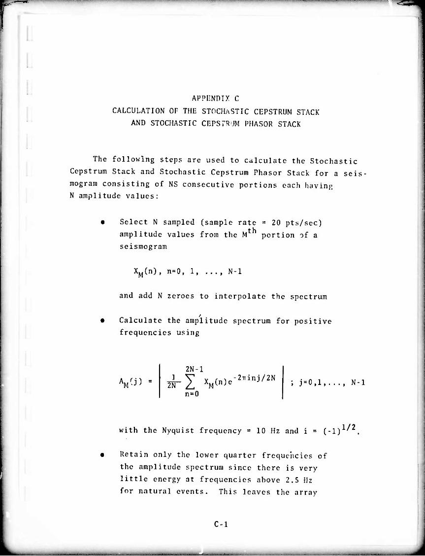
APPENDIX C

CALCULATION OF THE STOCHASTIC CEPSTRUM STACK

AND STOCHASTIC CEPSTR'JM PI1ASOR STACK

The following steps are used to calculate the Stochastic

Cepstrum Stack and Stochastic Cepstrum Phaser Stack for a seis

mogram consisting of NS consecutive portions each having

N amplitude values:

• Select N sampled (sample rate = 20 pts/sec)

amplitude values from the M portion of a

seismogram

XM(n) , n=0, 1, ..., N-l

and add N zeroes to interpolate the spectrum

• Calculate the amplitude spectrum for positive

frequencies using

VJ' ■ 2N-1

frl xM(„,o-^/2» n=0

; j=o,i, N-l

with the Nyquist frequency = 10 Hz and i ■ (-1) ' .

Retain only the lower quarter frequencies of

the amplitude spectrum since there is very

little energy at frequencies ahove 2,S Hz

fnr natural events. This leaves the array

C-l

1 « ■•• ' ' ^" " t'mm*im^^m^m ' ■ — ^■^^W^BWBi^^^—•^••^l^i^^«™^^—^ w^tmmmmmmimmmß t ^mmmmmmmmm

(AMCj), j = 0, 1, .... N/4-1)

Remove the mean and apply a cosinusoidal taper

11 to the first m and last 2(n of the A ai i i

giving the modified array

(AM (j), J = 0, 1 N/4-1)

The 2(n taper on the higher frequencies was used

to de-emphasize the higher frequencies

• Add N/4 zeroes to interpolate the cepstrum giving

the array

(AM ü), j = 0, 1, ..., N/2-1)

At this stage one would take the log of this AM array t0 ohtain the log cepstrum; but by not

using the log better results were obtained.

Calculate the Fourier Transform of the AK', array

using \\

FM(k)

N/2-1 1 Y A' mc-2^ijk/(N/2)

j = 0

C-2

^ —■ --■-■ — ■^^^p-

.

where (FMCk) , k = 0, 1 N/4-1) ar(

complex numbers representing the positive fre-

quency spectrum of AM. One can now obtain the

amplitude and phase of each cepstrum point k.

The array

( |F (k)|, k = 0, 1 N/4-1) is what we

is referred to as the cepstrum amplitude and the

complex numbers PyflO are referred to as cepstrum

phasors.

• To calculate the stochastic cepstrum stack, one

then calculates

|F (k)l = Max ( |rM(j)|, j = k-A/2, k+A/2)

for each section M and sums these over the number

of sections (NS) used from a given seismogram

(A is the stochastic window width). This gives

NS

C(k) ■ ^ |FM(k)l'WM M=l

whei' C(k) is the stochastic cepstrum stack and

W.. is a weighting factor, chosen such that the mean amplitude of each |FM(k)I array is equal.

C-3

Maa^k_^> —-i

To calculate the stochastic cepstrum phasor stack,

each FM(k) is replaced by FM(n) where n is the in-

dex of the Max value of |Py(j)| in the interval

j=k-A/2, k+A/2. The stochastic cepstrum phasor

stack is then defined by

NS

CP(k) I WM " VV M=l

C-4

J

.

APPENDIX D

SYNTHI-TIC SEISMOGRAMS

Synthetic scisniograms arc generated by passing white

noise through a recursive digital filter having a band pass

typical for seismic arrivals and adding this signal to itself

at delays tj and T2 (corresponding to pP-P and sP-p time

delays). The recursive digital filter was designed from

the following z-transform of a resonator with poles at

z=r iXp(iJM T) and a zero at q:

HU) 1 -qz -1

(l-2r(cosu)rT)z"1 + r2z"2)

For q=l this gives zero gain at M*0 and a resonant response

with u)r determining the resonant frequency and r relating to

the Q of the response. We used q=l, r=.9 and M =2* for the

generation of the synthetic data with T being the inverse of

the sample rate.

D-l

ad-a028 055 determination of seismic source depths …

Documents