AD-A144 SANTA BARBARA CA J BALTES ET AL. 31 MAY 84

i S GRC-CR-2-1091 F336i5-81-C-8108UNCLASSIFIED F/G 5/9 NL

* omhhhhmommmlsEohEohEohEEnhEEohmhhEEEEohhE

mhhmmmhsmhhu

VA. 'L.

LM I L

ll - mo

Lur

MICROCOPY RESOLUTION TEST CHARTNATIONAL BUREAU OF STANDARDS- 1963-A

pd

CR-2-1091

ENGAGE I- User's Manual

M.H. Tio enorJ.J. ae**

D.E. Bennett ,

Mwy01 1964

-:Po p aad fo, .mlwue.. .... 'ya(AS "

': I __ __ __]-

Cooumto.. P1 51 4.@ 08

GENERAL C A

RESEARCH CORPORATIO

C5 ~~P.O. BOX 6770, SANTA BARBARA, CALIFORNIA 91107

Tisgadon in an"~be qpw

84 OO&

0 1A

IiACKNOWLEDGMENTS

TThe authors are indebted to several co-workers and others for

their contributions, critiques and suggestions.

We would like to thank D. Nance and D. Curtis for editing andcomenting on the manuscript.

We would also like to thank Major R. Coffin, F. Campanile, J.

Kordik and R. Reboulet of ASD for the many useful suggestions on both

the computer program and this manual.

A special credit is also due to H. Jacobson, who developed theioriginal versions of the clutter scaling equations.Finally, our sincere appreciation to J. Phillips and P. Paciano .

for the excellent typing.

Aceenoion For

VT T 7

- .Codes

S'"/or -

Dizt , .c 1

.. , . .-

SeCUITV CLASSArICA~Oea of T.*s PAGE she 'e F en*

DOCUMENTATION READ INSTRUCT10%SJ. GSA SENATIPIEPAG BEFORE CO'1Pt.ETI. (, i -t.RM

CR-2-1091 O 9CALNISE4 TITLE (and Subfitle) S. TYPE OF REPORT b PERI,.D COVEnF,

Final Report

N ENGAGE II User's Hanual 0 PERFORMING ORG REPORT NUMSER

CR-2-10917 AUTPOORia, I CONTRACT OR GRANT NUMLRi. ..j

J. BalteB. E. Bennett F33615-81-C-0108

. M. H. Tichenor %2 PEAFORMING RGANIZATION NME &NO AORESS 10 PROGRAM ELEMENT PROJFT TA -

AREA & WORK UNjT NjMaeLk

General Research CorporationP.O. Box 6770Santa Barbara, California 93160-6770

* ,,.~ I CONTRO.LImG OFFICE NAME ANO AODRESS 12. REPORT DATE

Aeronautical Systems Division 5-31-84Wright Patterson Air Force Base, OH 45433 13 NUMBER OF PAES, ,'-150* 14 MONITORING AGENCY NAME ADOORESS(## dler.t iran Cntr,.l|ng Ofice) IS SECURITY CLASS (of ,h,s

Unclassified

aiso. DECLASSIFICATION OONGRAC. INC-." SCmEOULE

16. DISTRIBUTION STATEMENT (of this Report)

PUnlimited

L.17. DISTRIBUTION STATEMENT (of the absract entered in Black 20. it different from Report)

* '. IS. SUPPLEMENTARY NOTES

1S KEY WORDS (Continue on reverse side of necessary mid identfly by block number)

Air Engagement Air Radar RCSIntercept Process Missile SeekerTarget Interception ECM

%:5

5 .. 2 ABSTRACT (Cantonue an reverse side if necessary and Identify hv block number,

This user's manual describes ENGAGE II, a deterministic simulation ofan Air Interceptor vectored toward a target, detecting a target, maneuvering

I_ to attain a missile launch position, launching missiles at the targetand assessing their damage, and finally maneuvering into position tofire guns at the target. The model contains a 3 degree-of-freedom flightmodel for the AI, target, and missiles, and models both AI radar and a_ ,,j

Continued

DD I JAN3 1473 EDITION OF I NOV IS 1S OBSOLETE UNCLASSIFIED

SECURITY CLASSIFICATION OF Tm.S PAIE 017-e,, t,

*~~o br~**~.

UNCLASSIFIED_ugAjTY CLASIFICATION or THIS PAGeu(Sn OO rae",

Block 20 Continued

>Passive Track Adjunct for detection. It emphasizes the effects ofaircraft maneuverability, radar detection and tacking, and radarmissile detection when operating against targets with jammingcapabilities and low radar cross section._,-

,,.

°" .4

%II

5,

.5

01

UNCLASSIFIED

. . CUT CLAI. .ICA ION W THIS P&E'Wh., .... ..

-4.'.,-.- -.- ,-.-, -, ,,- ".,*', .,",'., ',a' ," t,"A,,. " - ?".. * ;,,, , ,, '. 5",.' - ' e .. . -'_. * . , : '.- " '.

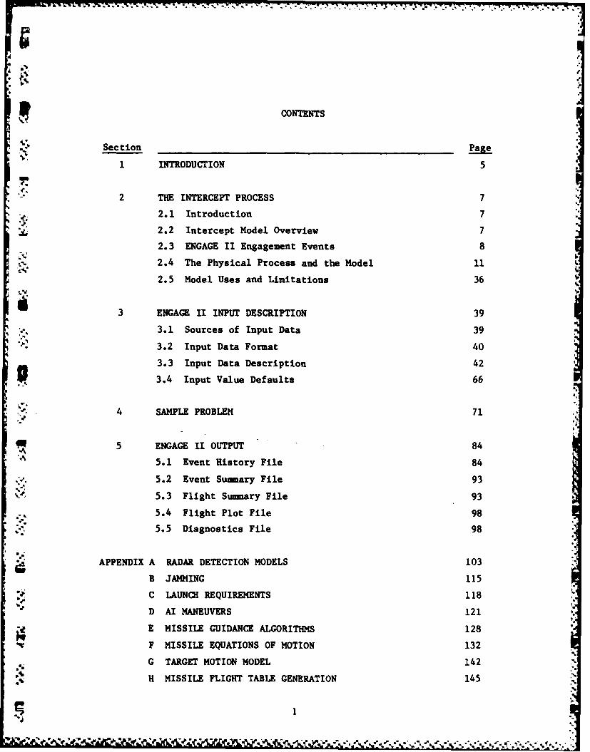
CONTENTS

Section __________________________ Page

1 INTRODUCTION 5

*-2 THE INTERCEPT PROCESS 7

2.1 Introduction 7

2.2 Intercept Model Overview 7

2.3 ENGAGE II Engagement Events 8

2.4 The Physical Process and the Model 11

2.5 Model Uses and Limitations 36

3 ENGAGE II INPUT DESCRIPTION 39

3.1 Sources of Input Data 39

3.2 Input Data Format 40

3.3 Input Data Description 42

P3.4 Input Value Defaults 66

V4 SAMPLE PROBLEM 71

5 ENGAGE II OUTPUT 84

5.1 Event History File 84

5.2 Event Sunmmary File 93

5.3 Flight Summasry File 93

5.4 Flight Plot File 985.5 Diagnostics File 98

*APPENDIX A RADAR DETECTION MODELS 103 a

B JAMMING 115

C LAUNCH REQUIREMENTS 118

b.D AI MANEUVERS 121

E MISSILE GUIDANCE ALGORITHMS 128

F MISSILE EQUATIONS OF MOTION 132

G TARGET MOTION MODEL 142

H MISSILEnFIGHT TABLE GENERATION 145

-- A

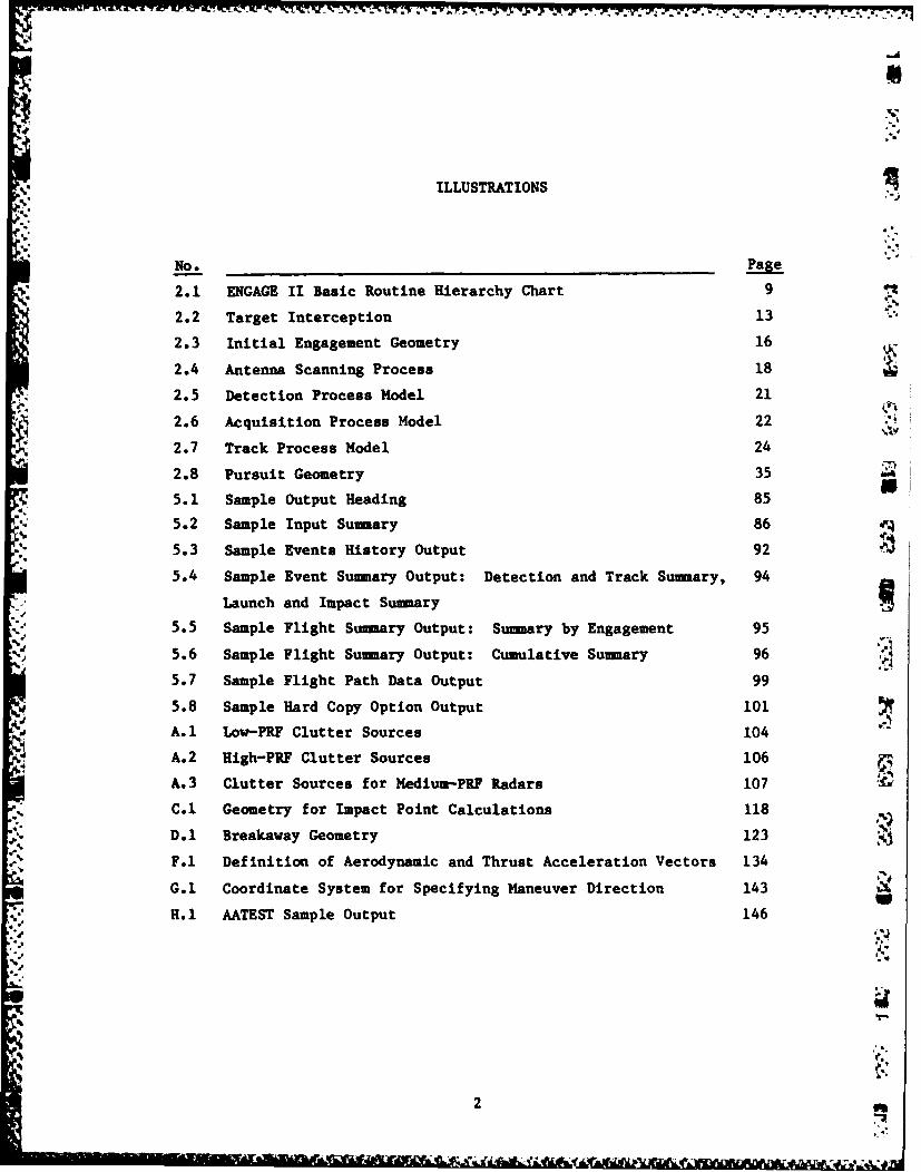
ILLUSTRATIONS

No. Page

2.1 ENGAGE II Basic Routine Hierarchy Chart 9

2.2 Target Interception 13 -'

2.3 Initial Engagement Geometry 16

2.4 Antenna Scanning Process 18

2.5 Detection Process Model 21

2.6 Acquisition Process Model 22

2.7 Track Process Model 24

2.8 Pursuit Geometry 35

5.1 Sample Output Heading 85

5.2 Sample Input Summary 86

5.3 Sample Events History Output 92

5.4 Sample Event Summary Output: Detection and Track Summary, 94

Launch and Impact Summary

5.5 Sample Flight Summary Output: Summary by Engagement 95

5.6 Sample Flight Summary Output: Cumulative Summary 96

5.7 Sample Flight Path Data Output 99

5.8 Sample Hard Copy Option Output 101

A.1 Low-PIP Clutter Sources 104

A.2 High-PRF Clutter Sources 106

A.3 Clutter Sources for Medium-PRF Radars 107

C.A Geometry for Impact Point Calculations 118

D.1 Breakaway Geometry 123 MF.1 Definition of Aerodynamic and Thrust Acceleration Vectors 134

G.1 Coordinate System for Specifying Maneuver Direction 143

H.l AATEST Sample Output 146

2

- 4...........

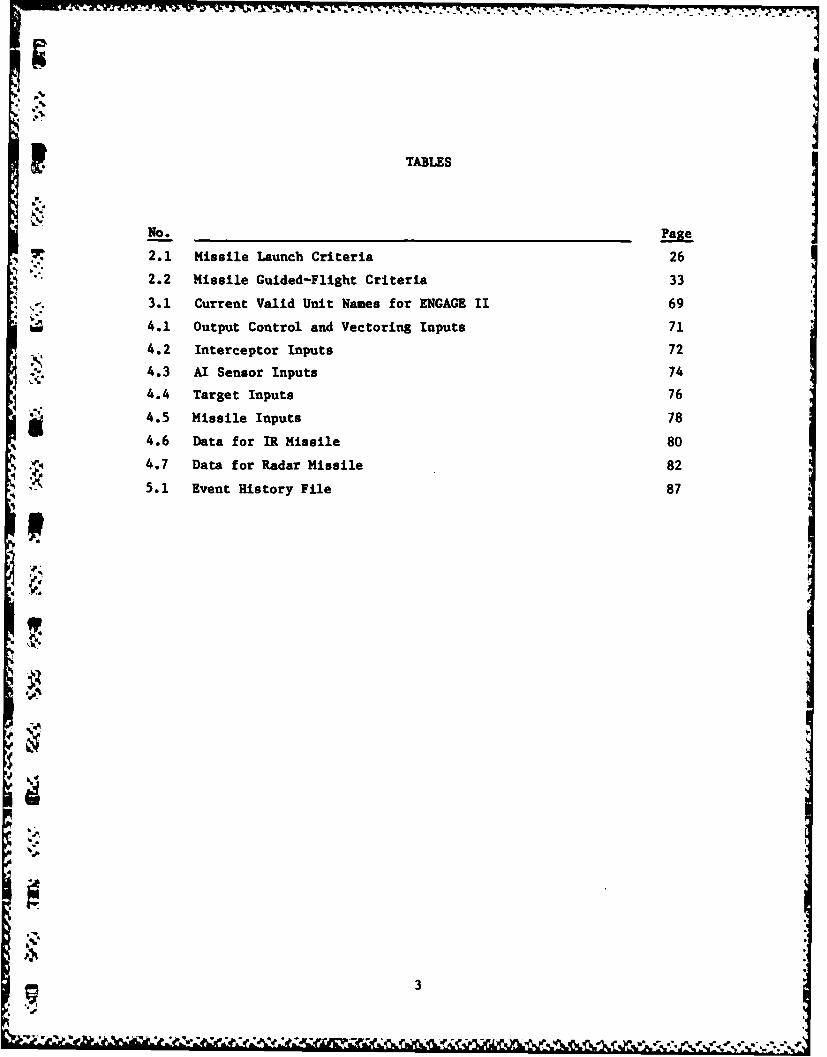
TABLES

7 2.1 Missile Launch Criteria 262.2 Missile Guided-Flight Criteria 33

, 3.1 Current Valid Unit Names for ENGAGE II 694.1 Output Control and Vectoring Inputs 71

4.2 Interceptor Inputs 72

4.3 AI Sensor Inputs 74

4.4 Target Inputs 76

4.5 Missile Inputs 78

4.6 Data for IR Missile 80

I IP 4.7 Data for Radar Missile 82

5.1 Event History File 87

V

i'S

3

-. . t ........... ............. S6A

% 44

(This page intentionally blank)

'--,

I

Ki

4

- INTRODUCTION

The ENGAGE II computer model was developed for the Aeronautical

Systems Division of USAF/AFSC to enable them to assess the ability of

modern interceptor aircraft armed with guided missiles and guns to

' attack maneuvering targets. The model is a major extension of theFIPDC and ENGAGE models that General Research has been developing

since 1977.

Program ENGAGE II simulates the process of an airborne

'J* interceptor (AI) receiving vectoring toward the intended target,

attempting to detect the target, maneuvering to attain a missile launch

position, launching missiles at the target, and finally reaching a

position to fire guns at the target. Program ENGAGE II treats each of

these phases in some detail, emphasizing the aspect dependent nature of

the target's detectability, the effects of jamming and ground clutter on

the AI radar, and the maneuverability of the AI and missiles. The model

Aincludes a three degree-of-freedom flight model for the interceptor,target and missiles. The program considers the dynamic geometry and

,' missile fly-out characteristics to calculate proper lead angles for

missile flight. Active and semi-active radar missiles and passive (IR)

% missiles are modeled. The interceptor flight model includes the

capability to break away and reattack from the stern, using rear-

SIVhemisphere missiles and guns.

* *Detection is achieved by either the fighter radar or a passive

' search set. The program is capable of modeling multi-mode radar and

accounts for the effects of ground clutter, aspect-dependent radar cross

section of the target, and electronic countermeasures (ECM). The

passive search set is sensitive to range and target aspect, but is

assumed to be unaffected by clutter or ECM.

5

767_7 7 .- ,.. 17

The purpose of this User 's Manual is to provide non-programming

users of ENGAGE II with the information necessary to use the model

effectively. Because no other documentation is being prepared for this

model, mathematical treatments of radar detection, jamming, missile

launch conditions, and AI, missile and target flight are included in the

appendices. Section 2 of this manual describes the processes that are

modeled and the implementation of the modeling. Section 3 describes the

input and Section 4 includes a sample problem. The various types of

output of the program are described in Section 5.

10

wy5;A)

.'4 ......

2 THE INTERCEPT PROCESS

This section describes the physical system of the intercept

' process and its implementation in the computer model ENGAGE II. Section

2.1 provides an introduction, Sec 2.2 provides an overview of the

simulation model, Sec 2.3 lists and briefly describes the major events

modeled in the intercept process, and Sec 2.4 describes the basic

program flow. Section 2.5 mentions some of the uses and limitations of

the model. Throughout this section, when references are made to proo-am

inputs, the input name is included in capital letters within

parentheses.

2.1 INTRODUCTION

Program ENGAGE II is a deterministic simulation of a fighter

aircraft being vectored toward a target, detecting it, maneuvering to

attain a missile launch position, launching missiles at the target, and

S finally reaching a position to fire guns at the target. ENGAGE 11 is a

three-degree-of-f reedom simulation of aircraft and missile flight, and

can thus provide a graphic picture of the interception process. No

*.. random numbers are used in the simulation. Instead, probabilities are

- calculated and integrated numerically, and the program will output the

probability of the fighter's detecting a target and converting to a

firing position-the well-known probability PDC-and the probability

that the missiles launched will destroy the target, the probability of

.~ 480k ll K

" ~2.2 INTERCEPT MODEL OVERVIEW

The model is designed to allow the user to generate an average PDC

for a scenario by automatically running a series of engagements at

different geometries, and then averaging the result. The user defines

the number of Heading Crossing Angles (NHCA) and the number of Offsets

(HOFF). An engagement is generated for each Heading Crossing Angle and

Offset combination. The Heading Crossing Angles are input by the user.

7

The offsets may be input (IOFDIS -2) by the user, or they may be

1 generated by the program from a single nominal input distance (OFF(1))

f or either a uniform distribution (IOFDIS -0) or a normal distribution

(IOFDIS - 1).

I.%

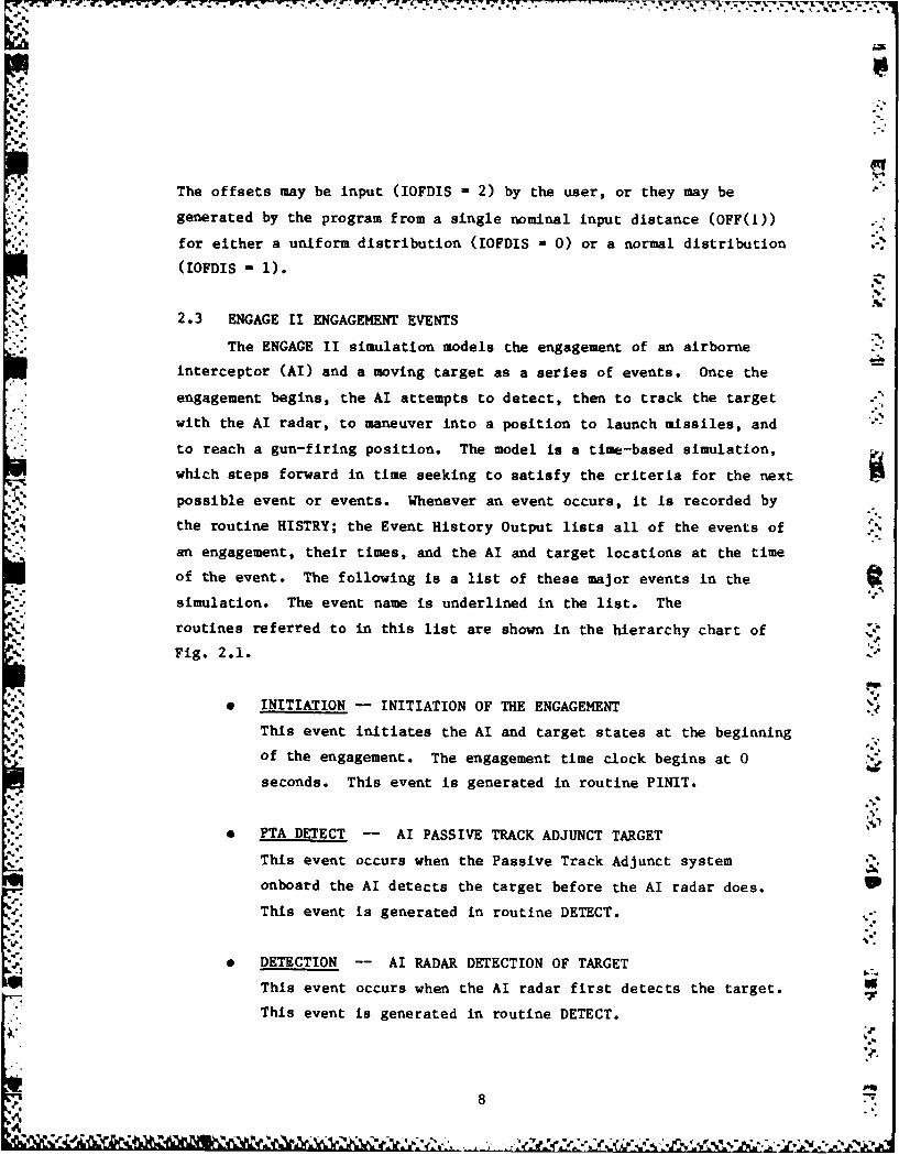
2.3 ENGAGE II ENGAGEMENT EVENTS

* The ENGAGE II simulation models the engagement of an airborne

interceptor (AI) and a moving target as a series of events. Once the

engagement begins, the AI attempts to detect, then to track the target

* with the AI radar, to maneuver into a position to launch missiles, and

to reach a gun-firing position. The model is a time-based simulation,

which steps forward in time seeking to satisfy the criteria for the next

possible event or events. Whenever an event occurs, it is recorded by

the routine HISTRY; the Event History Output lists all of the events of

an engagement, their times, and the AI and target locations at the time

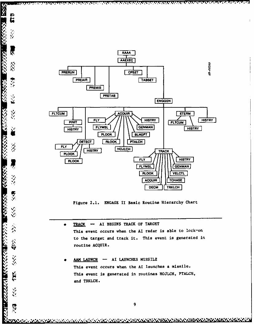
of the event. The following is a list of these major events in the

* simulation. The event nam is underlined in the list. The

routines referred to in this list are shown in the hierarchy chart of

*1Fig. 2.1.5

0 INITIATION -- INITIATION OF THE ENGAGEMENT

4 This event initiates the AI and target states at the beginningof the engagement. The engagement time clock begins at 0

seconds. This event is generated in routine PINIT.

4 PTA DETECT -- Al PASSIVE TRACK ADJUNCT TARGET

This event occurs when the Passive Track Adjunct system

onboard the AI detects the target before the AI radar does.

This event is generated in routine DETECT.

* DETECTION -- AI RADAR DETECTION OF TARGET

S This event occurs when the AI radar first detects the target.

This event is generated in routine DETECT.

8 7

4

PRRN _4PE

r* PREA

4.L'I PR.M

FPRETA8

FLYMSL GENMAN

RLOK VLCT

PLO ACQUIY RAC A

fe .F D EC M R L I

4. Figure 2.1. ENGAGE II Basic Routine Hierarchy Chart

*. TRACK - AI BEGINS TRACK OF TARGET

4'- This event occurs when the AI radar is able to lock-on

to the target and track it. This event is generated in

routine ACQUIR.

. AAM LAUNCH -- Al LAUNCHES MISSILE

This event occurs when the AI launches a missile.

This event is generated in routines HOJLCH, PTALCH,

and TRKLCH.

9

-•.. . - • SIss s s s s s s s s s s s s s s s s - .e -.- ° °

i.

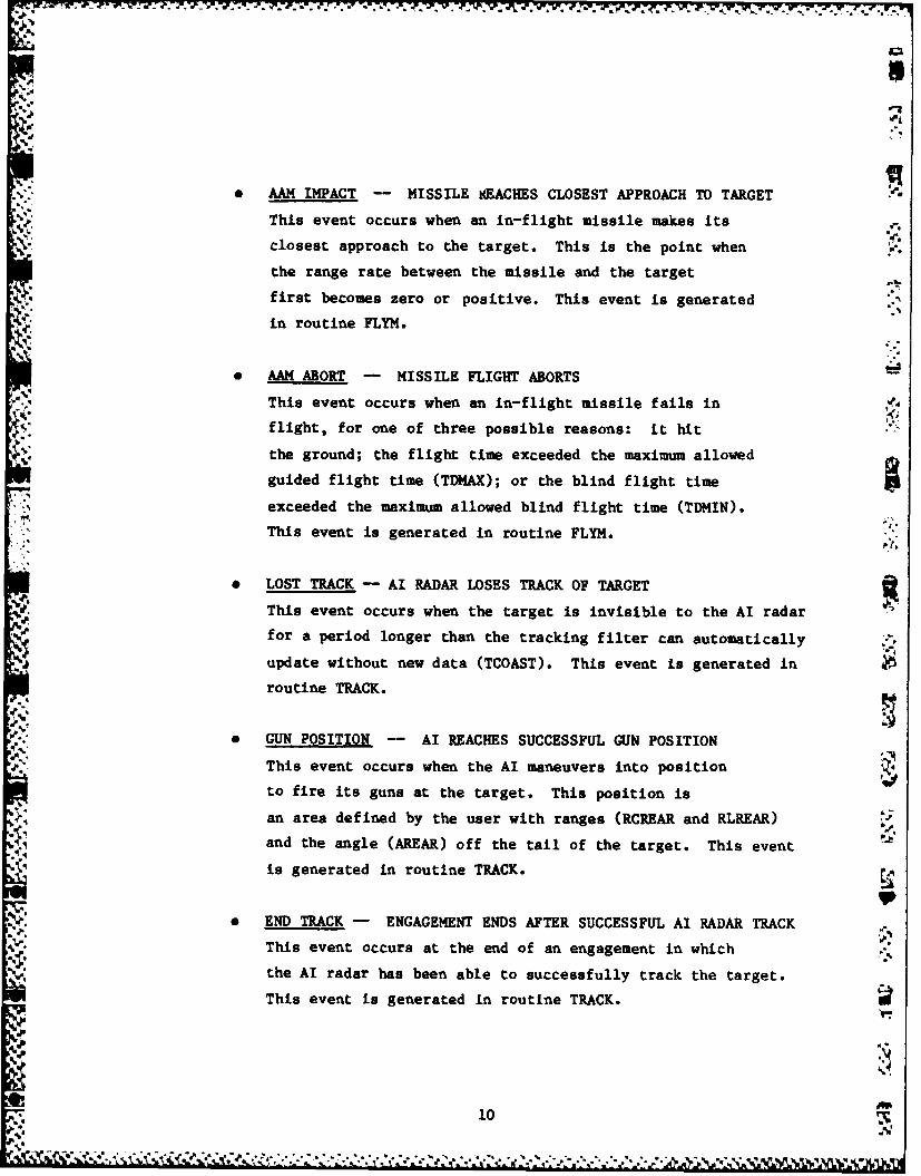
. AAM IMPACT -- MISSILE kEACHES CLOSEST APPROACH TO TARGET

This event occurs when an in-flight missile makes its

V-i closest approach to the target. This is the point when S.

the range rate between the missile and the target

first becomes zero or positive. This event is generatedin routine FLYM.

* AAM ABORT - MISSILE FLIGHT ABORTS

This event occurs when an in-flight missile fails in

flight, for one of three possible reasons: it hit

the ground; the flight time exceeded the maximum allowed

guided flight time (TDMAX); or the blind flight time

exceeded the maximum allowed blind flight time (TDMIN).

This event is generated in routine FLYM. ".

* LOST TRACK -- AI RADAR LOSES TRACK OF TARGET

This event occurs when the target is invisible to the AI radarfor a period longer than the tracking filter can automatically

update without new data (TCOAST). This event is generated in

routine TRACK.

" GUN POSITION -- AI REACHES SUCCESSFUL GUN POSITION

.; This event occurs when the AI maneuvers into position

to fire its guns at the target. This position is

an area defined by the user with ranges (RCREAR and RLREAR) '5

and the angle (AREAR) off the tail of the target. This event

is generated in routine TRACK.

. END TRACK -- ENGAGEMENT ENDS AFTER SUCCESSFUL AI RADAR TRACK

-; This event occurs at the end of an engagement in which

vthe AI radar has been able to successfully track the target.

This event is generated in routine TRACK.

IF"

10

* NO DETECT -- ENGAGEMENT ENDS WITH NO DETECTION

* This event occurs at the end of an engagement in which

the AI has not detected the target with either the AI

radar or the Passive Track Adjunct. This event is generated

in routine DETECT.

. ONy PTA - ENGAGEMENT ENDS WITH PASSIVE TRACK ADJUNCT

TARGET DETECTION, BUT NO AI RADAR DETECTION

Thi evntoccurs at the end of an engagement in which

the AI Passive Track Adjunct has successfully detected the

target, but the AI radar has not. This event is generated in

routine DETECT.

0 DET NO TRK - ENGAGEMENT ENDS WITH AI RADAR DETECTION,

BUT NO AI RADAR TRACK

This event occurs at the end of an engagement in which

the AI radar has detected the target, but has not been

able to establish a track on it. This event is generated in

* routine ACQUIR.

- TERMINATION -- ENGAGEMENT SUMMARY

4 This event occurs after the end of the engagement. The model

~ Y assures that all missiles launched during the engagement

either have reached closest approach or have aborted,

then calculates the Probability of Kill, PK, for the

engagement. This event is generated in routine ETERM.

2.4 THE PHYSICAL PROCESS AND THE MODELI 2.4.1 Introduction

The process of target interception has the following phases:

0 GCI Vectoring

In this phase, the AI is under the control of a vectoring

agency and is on an approximately collision, non-maneuvering

course with the target. This phase end. after the AI detects

the target and declares its independence from the vectoring

agency.

* Conversion

In this phase, the AI begins to follow the target with

its own onboard receiving devices, obtains steering

information, and eventually launches air-to-air missiles

(AAMs). This phase ends at the first AAM launch.

0 Attack

In this phase, the AI continues to maneuver to maintain

the proper course for further AAM launches and support

for in-flight missiles, if they employ semi-active radar

seekers.* This phase includes the assessment of AAM

launches and the launch of subsequent missiles. The

AI will attempt to convert to a stern attack to launch

rear-aspect IR missiles, if the original attack is

from the front and the IR missiles have no forward-hemisphere

* capability. If the AI is carrying guns, the AI will attempt

to maneuver to a stern gun-firing position. The phase ends

when all missiles have been launched and a gun-firing position4

has been achieved; when the target is lost; or when the AI has

exceeded its maximum engagement flight time. ',

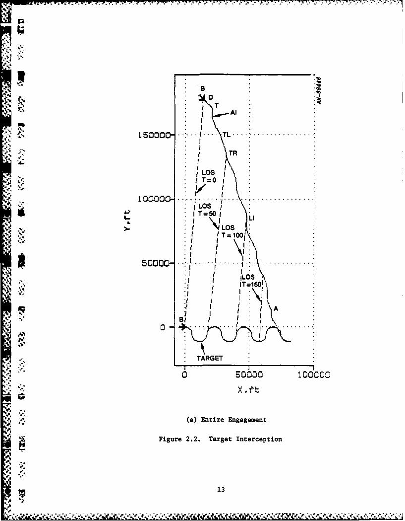
* Figure 2.2 illustrates the process of target interception. The

* entire engagement is illustrated in the first plot. The initial

vectoring conditions are defined by a 45 degree Heading Crossing Angle

and a 5000 foot offset, assuming the target flight is straight with no

velocity change. The target, however, is maneuvering in a sinusoidal

12

BXD1* -Al

T

15000" " TL

.,. It

,1.OSI T=O

OLOS6 iT=50~

Ia T 1001

*1 I

5oooo- ..:. ..... ' ... .~ ~ ..............

44 o EDOD 10000

CAA

:0 6 0 0 i : C- : 0

? , (a) Entire Engagement

Figure 2.2. Target Interception

I:I

" ',..,;'

.,j." -. '*, .. ''. ,v ¢ .' '.; ";', , .' + 7,V . ',g4;.2 ,;;,+,"£ ,,"4, , ., "

Al

ILAUNCH (Li)

0 .. ... . .... ............ ........ ...

6 ....

4 0 0 0 0 -.. . ... . . .. . , ° ° ° ° , ° . . . . . ." . . . . . . . . . . .:

2 , . 0000- .......... BORT (A): ...........

I L4

TARGETGUN ,

- 2 0 0 0 .... " ......., ...• -. ..........I ............ "

3-000 6r: , -3 0

X Iw* d..

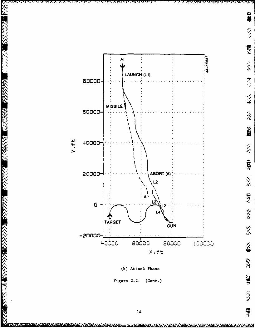
(b) Attack Phase '

Figure 2.2. (Cont.)

-J-

414

4* 77

pattern at the bottom of the plot. The dashed lines represent lines of

- sight every 50 seconds. The engagement begins at B, and detection

occurs at point D. Track begins at point T, then is lost briefly at

point TL when Signal-to-Interference drops below threshold, and is

regained at TR. The wavering path of the AI is due to the changing aim

'~ point based on the straight-line projection of the target flight path.

Eventually, all missiles on board are launched and successful gun

position is reached. The flight then terminates. The second plotillustrates the missile launches (dashed lines), and begins at the first

radar missile launch point LI. This launch is based on a straight-line

projection of the target flight, which would have indicated a nearly

head-on collision in the middle of the plot. Instead, the targetmaneuvers kept the target beyond the maximum guided flight time allowed

** .~.the radar missile, and it aborted at point A. The second radar missile

'S ~ launch, point L2, immediately after the assessment of the first

* missile's abort, is successful at point 12. Both IR missiles are then

N launched at points L3 and L4., and impact before the AI reaches gun

position, point GUN.

The remainder of this section will discuss the target interception

4 %'. process in more detail, as it is implemented in the simulation.5%

2.4.2 GCI Vectoring

The model-user provides the information to establish the beginning

of the engagement, which simulates the GCI vectoring instructions for

the AI. These user inputs also establish the errors in the GCI

vectoring instructions. These inputs include the Heading Crossing Angle

(UCA) between the headings of the AI and the target, the offset (OFF) of

the AI from a collision course, the lag (DUAG) of the the target from a1%0 ~d V collision course, and the initial distance between the Al and the target

%S at the beginning of the engagement (RO and RPI, the initial ranges for

HCA - 0 degrees and HCA - 180 degrees, respectively.) The range at the

beginning of the engagement, assuming no offset, is interpolated from RO

15

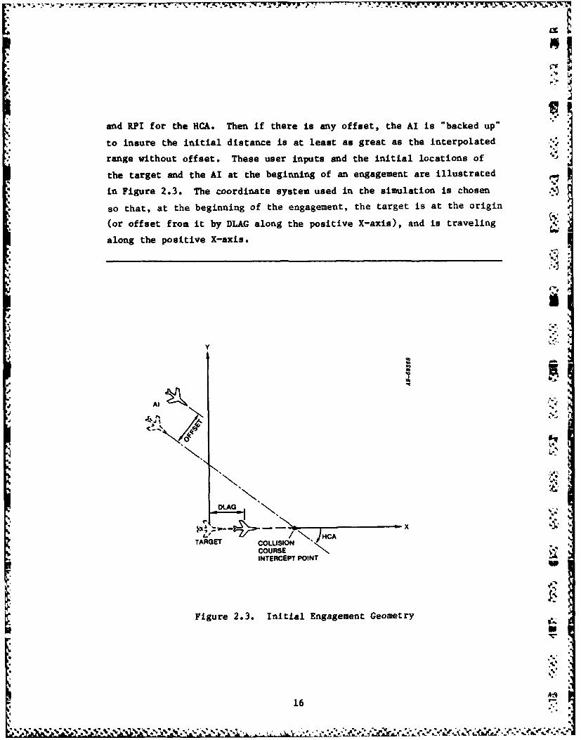
and RPI for the HCA. Then if there is any offset, the AI is "backed up"

to insure the initial distance is at least as great as the interpolated 1!Irange without offset. These user inputs and the initial locations of

the target and the AI at the beginning of an engagement are illustrated

in Figure 2.3. The coordinate system used in the simulation is chosen

so that, at the beginning of the engagement, the target is at the origin

(or offset from it by DLAG along the positive X-axis), and is traveling

along the positive X-axis.

Al

OLAG

\..

x)' HCA

TARGET COLLISION "'COURSE KINTERCEPT POINT

Figure 2.3. Initial Engagement Geometry

16

[.':.';V ,,' ,',' ,'',','..,.' ','.''. . ".,'v.,. ., ,.,.... • """ " . •.": . .. " . . . " ":..

The AI, once given the initial GCI vectoring instructions,

continues in a straight path until detection. The target may maneuver

at any time, as the user defines in the target maneuver inputs. At the

beginning of the engagement, all receiving equipment onboard is on,

attempting to detect the target. The AI has 3 methods of detection: Al

Radar detection; Passive Track Adjunct Detection; and Track-on-jam

Detection. Each of these will be described in detail.

AI Radar Detection. The AI radar model in ENGAGE II computes the

signal-to-interference ratio within the AI radar at each scan across the

target and deduces a detection probability on each scan. These

probabilities are accumulated to derive the cumulative detection

probability. The interference includes mainlobe clutter residing

outside the passband of the doppler filter containing the target,

IN sidelobe clutter inside the passband, and the thermal noise inside the

passband. Appendix A describes the meaning of these clutter categories.

The dependence of clutter upon the doppler frequency of the target

signal and the dependence of mainlobe clutter upon the beam depression

IN angle are both accounted for. If the target has jamming capability, the

signal-to-interference ratio also includes the noise Jaming. This and

9 other types of ECM included in the model are described in Appendix B.

The simulation accommodates radars of a pure waveform, or

those with time-shared waveforms, which interleave low-PRF, medium-PRF,

and high-PRF wavefirms. These waveforms differ in the model in the

effects of in-band and mainlobe clutter. Appendix A describes these

differences. The model-user provides parameters for all those waveforms

available on the AI radar, and the model determines the best (highest

signal-to-interference ratio) waveform of those available to attempt

detection.

1i7t

17 -

.. %V...%

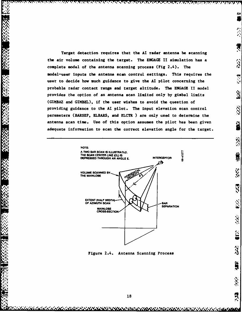
Target detection requires that the AI radar antenna be scanning

the air volume containing the target. The ENGAGE II simulation has a

,d complete model of the antenna scanning process (Fig 2.4). The

model-user inputs the antenna scan control settings. This requires the

user to decide how much guidance to give the AI pilot concerning the

probable radar contact range and target altitude. The ENGAGE II model

provides the option of an antenna scan limited only by gimbal limits

(GIMBAZ and GIMBEL), if the user wishes to avoid the question of

providing guidance to the AI pilot. The input elevation scan control

parameters (BARSEP, ELBARS, and ELCTR ) are only used to determine the

antenna scan time. Use of this option assumes the pilot has been given

adequate information to scan the correct elevation angle for the target.

NOTE:A TWO BAR SCAN IS ILLUSTRATh:V.THE SCAN CENTER LINE (CL) ISDEPRESSED THROUGH AN ANGLE E. INTERCEPTOR

VOLUME SCANNED DY ,THE MAINLODEE

Al

EXTENT (HALF WIOTHOF AZIMUTH SCAN SA

MAINLOESEPARATION

CROSS-ECTION

,1' Figure 2.4. Antenna Scanning Process

18

N. )AONa

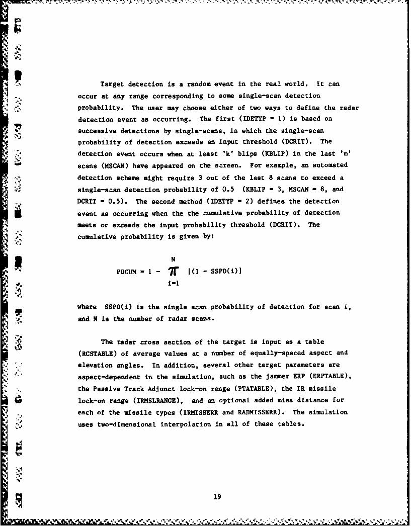
Target detection is a random event in the real world. It can

- occur at any range corresponding to some single-scan detection

., 1-s.probability. The user may choose either of two ways to define the radar

detection event as occurring. The first (IDETYP - 1) is based on

successive detections by single-scans, in which the single-scan

probability of detection exceeds an input threshold (DCRIT). The

' "detection event occurs when at least 'k' blips (KBLIP) in the last 'im'

scans (MSCAN) have appeared on the screen. For example, an automated

detection scheme might require 3 out of the last 8 scans to exceed a

single-scan detection probability of 0.5 (KBLIP - 3, MSCAN - 8, and

DCRIT - 0.5). The second method (IDETYP - 2) defines the detection

event as occurring when the the cumulative probability of detection

meets or exceeds the input probability threshold (DCRIT). The

!cumulative probability is given by:

N

PDCUM - 1- 7r [(1 - SSPD(i)].14 i-I

where SSPD(i) is the single scan probability of detection for scan i,

'and N is the number of radar scans.

The radar cross section of the target is input as a table

(RCSTABLE) of average values at a number of equally-spaced aspect and

* 'elevation angles. In addition, several other target parameters are

aspect-dependent in the simulation, such as the jammer ERP (ERPTABLE),

the Passive Track Adjunct lock-on range (PTATABLE), the IR missile

lock-on range (IRMSLRANGE), and an optional added miss distance for

each of the missile types (IRMISSERR and RADMISSERR). The simulation

uses two-dimensional interpolation in all of these tables.

91

o tabes

7777777. 7, 7. 77° 7 . '71 la,

*Passive Track Adjunct Detection. The AI may have a Passive Track

Adjunct (PTA) onboard to aid in target detection. This capability is

modeled in two modes, Radar Clue Mode (PTATYP - 1) and Autonomous Mode

(PTATYP - 2). Detection is based on a target-aspect-dependent lock-on

range, input by the user (Table PTATABLE). The model requires the

target to be within user-input scan limits (PAZSCN and PELSCN) for

successful detection. If the PTA is in Radar Clue Mode and successfully

detects the target, the PTA provides the AI radar with a better

prediction of the target location, and the AI radar can narrow its own

scan limits. This is modeled by reducing the AI radar scan period to a

refined AI radar scan period (TSTA2R) that the user inputs. If the PTA

is in Autonomous Mode and successfully detects the target, then after a

delay (TSTARE) to provide time to determine the target range, the AI

pilot has enough information (range and angle) to begin the conversion

*phase; to steer toward the target, and to attempt to launch missiles.

The model assumes the range rate is unknown, however, so no lead

predictions are made. See Appendices C and D for descriptions of

maneuvers and aimpoints.

Home-on-Jam Detection. If the target is actively jamming, and the

AI radar has the capability to track a jamming signal, then detection

can occur when the jamming signal is above the track-on-jam threshold

(TTOJ). The track-on-jam radar mode can give the pilot enough

information (angle, but not range or range rate) to begin the conversion

phase; to steer toward the target, and to attempt to launch missiles.

Since the model assumes that only the target angle is known, the missile

is aimed directly at the target.

Detection, then, can be accomplished by the AI radar in a clear

environment, or by burnthrough in a jamming environment (providing

target angle, range, and range rate); or by an onboard Passive Track

Adjunct (providing target angle and range); or by the

20 WI

. , ,

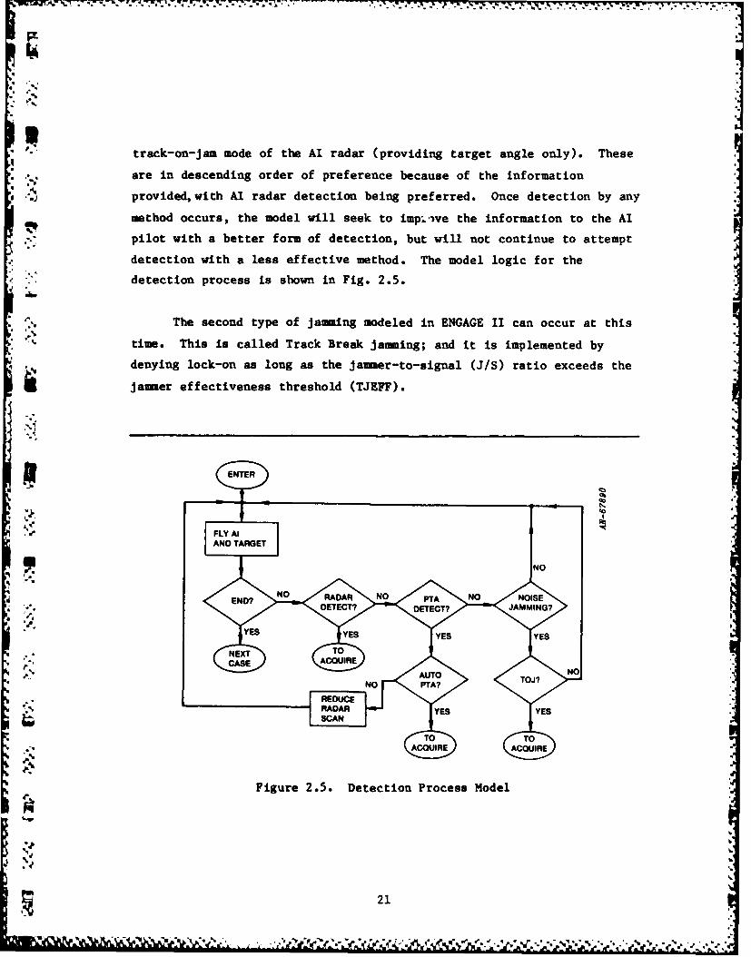
track-on-jam mode of the AI radar (providing target angle only). These

are in descending order of preference because of the information

provided, with Al radar detection being preferred. Once detection by any

method occurs, the model will seek to impi.,we the information to the AI

pilot with a better form of detection, but will not continue to attempt

detection with a less effective method. The model logic for the

detection process is shown in Fig. 2.5.

C. The second type of jamming modeled in ENGAGE II can occur at this

" 'time. This is called Track Break jamming; and it is implemented by

denying lock-on as long as the ja-.er-to-signal (J/S) ratio exceeds the

jammer effectiveness threshold (TJEFF).

I,,

5-.-

,, FLY AlAND TARGET

DETECT? 7DETt JAMMING?

S""YES Y'ES YESYE

,

t-!-

RADAR YES YESi SCAN

%

•Figure 2.5. Detection Process Model

.46"

%.%

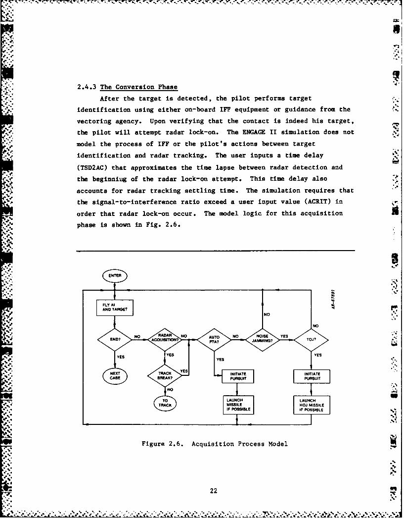
2.4.3 The Conversion Phase

After the target is detected, the pilot performs target

identification using either on-board IFF equipment or guidance from the

vectoring agency. Upon verifying that the contact is indeed his target,

the pilot will attempt radar lock-on. The ENGAGE II simulation does not

model the process of IFF or the pilot's actions between target

identification and radar tracking. The user inputs a time delay

(TSD2AC) that approximates the time lapse between radar detection and

* ~the beginniug of the radar lock-on attempt. This time delay also

accounts for radar tracking settling time. The simulation requires that

the signal-to-interference ratio exceed a user input value (ACRIT) in

order that radar lock-on occur. The model logic for this acquisition

phase is shown in Fig. 2.6.

.'.1! AND TARGET

END? ACCUISITON? PTJAMMING? TOJ? .

YE E ES Y.,ES

NEXT TRACK YE INITIATE IIIT

CSBREA TT 10TAKMISSILEHOMISL

Figure 2.6. Acquisition Process Model

P-

22

, :" -'e" -. "* ."' "% . " " . " . . . . . ". .* . . -

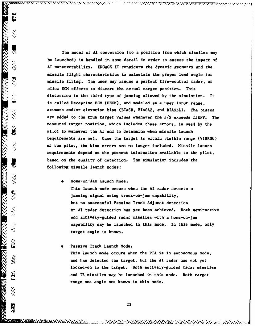
The model of AI conversion (to a position from which missiles may

" be launched) is handled in some detail in order to assess the impact of

,. AI maneuverability. ENGAGE II considers the dynamic geometry and the

missile flight characteristics to calculate the proper lead angle for

missile firing. The user may assume a perfect fire-control radar, or

allow ECK effects to distort the actual target position. This

distortion is the third type of jamming allowed by the simulation. It

is called Deceptive ECM (DECM), and modeled as a user input range,

--- azimuth and/or elevation bias (BIASR, BIASAZ, and BIASEL). The biases

., ~-are added to the true target values whenever the J/S exceeds TJEFF. The

measured target position, which includes these errors, is used by the

pilot to maneuver the AI and to determine when missile launch

• • requirements are met. Once the target is within visible range (VISRNG)

'4 of the pilot, the bias errors are no longer included. Missile launch

requirements depend on the present information available to the pilot,

based on the quality of detection. The simulation includes the

following missile launch modes:

- " Home-on-Jam Launch Mode.

This launch mode occurs when the AI radar detects a

jamming signal using track-on-jam capability,

but no successful Passive Track Adjunct detection

* or AI radar detection has yet been achieved. Both semi-active

and actively-guided radar missiles with a home-on-jamcapability may be launched in this mode. In this mode, only

- "target angle is known.

* Passive Track Launch Mode.

This launch mode occurs when the PTA is in autonomous mode,

and has detected the target, but the AI radar has not yet

locked-on to the target. Both actively-guided radar missiles

and IR missiles may be launched in this mode. Both target

range and angle are known in this mode.

23• 'i,

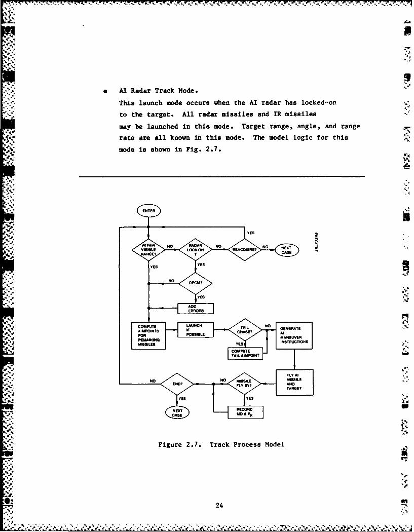
AI Radar Track Mode.

This launch mode occurs when the AI radar has locked-on

to the target. All radar missiles and IR missiles

may be launched in this mode. Target range, angle, and range

rate are all known in this mode. The model logic for this

mode is shown in Fig. 2.7.

THIN" No RAA O NO NEXT

OVISLE LOCKON REACAUIRE?

YES YESS

NO NO MISSIL

ADND

IF TAILEN

Al 2.7 TrAc E s l2F -S

REMAIING MNEUVEINTRCTON

MISIESYE

COMPUTE

TAIL AMP04N

.4-J

Figure 2.7. Track Process Model

.CT

24

Only one missile may be in-flight for any launch mode. However,

if the launch mode changes, then a missile may be launched as soon as

the new launch criteria are met, even if there are missiles still in

flight from earlier launch modes.

There are two types of missiles on board the AI: IR and radar

-. missiles (IRMIS and RADMIS). Each has a specific set of requirements

which must be met before launch can occur; these launch requirements,

- which depend on both missile launch mode and missile type, are listed

in Table 2.1. Both missile types must detect the target for a

successful flight. Detection by the IR missile seeker requires the

" target line-of-sight to be within the scan limits of the seeker

(GIMBMX(IRMIS)) and the range to the target to be within the IR missile

detection range (table IRMSLRANGE.) The radar missile seeker lock-on

requires that the target line-of-sight be within the scan limits of the

seeker (GIMBMX(RADMIS)) and that the signal-to-interference ratio beP adequate (SIRAAM). The model of the radar missile seeker is the same as

- :that used for the AI high-PRF radar, described in Appendix A. All the

cited sources of clutter and noise interference are considered. Missile

it launch is inhibited if the AI or the missile seeker are in their

_ *1 respective regions where mainlobe clutter (in-band mainlobe clutter) is

present.

The ENGAGE II simulation handles two types of radar missiles-

V .those that require lock-on before launch (or shortly thereafter), and

are semi-actively guided (AAMTYP=1), and those with active seekers that

can lock on much after launch (AAMTYP'2). Both types of missiles must

pass the same types of test for a successful flight. However, ther semi-active type of missile must have seeker lock-on at the time of

- , launch, while the active type of missile may wait until a specified time

(TSAACQ) before the expected impact.

25

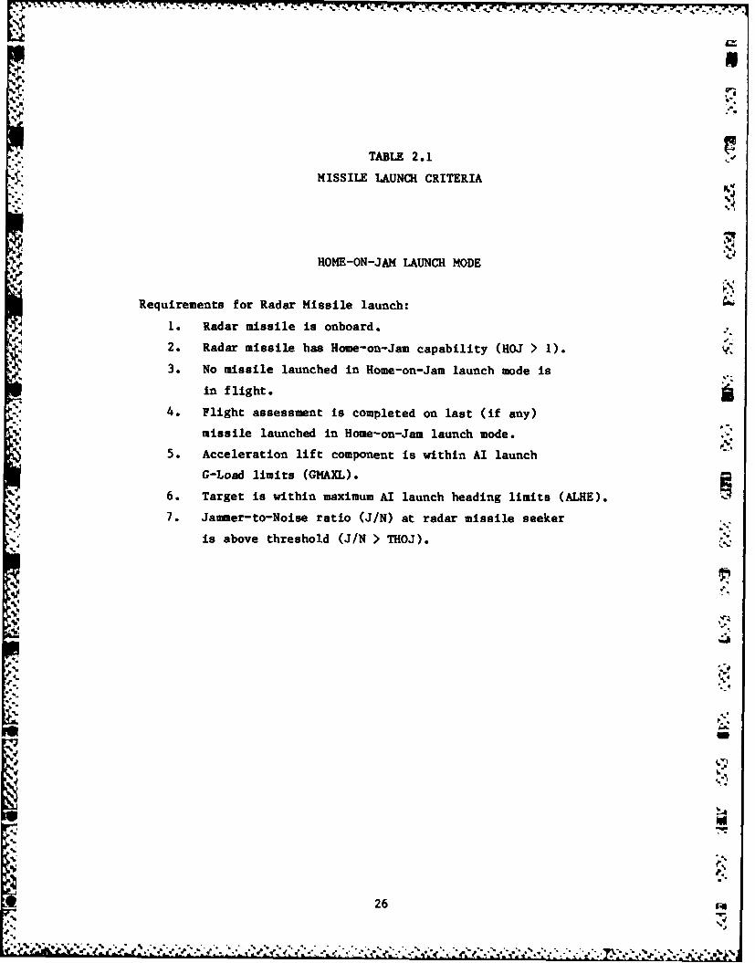
TABLE 2.1

MISSILE LAUNCH CRITERIA

HOME-ON-JAM LAUNCH MODE

Requirements for Radar Missile launch:

1. Radar missile is onboard.

2. Radar missile has Home-on-Jam capability (HOJ > 1). f.

3. No missile launched in Home-on-Jam launch mode is

in flight.

4. Flight assessment is completed on last (if any)

missile launched in Home-on-Jam launch mode. -

5. Acceleration lift component is within AI launch

G-Load limits (GMAXL).

6. Target is within maximum AI launch heading limits (ALHE).

7. Jammer-to-Noise ratio (J/N) at radar missile seeker

is above threshold (J/N > THOJ).

.-A

.-s

26 l

-' . Z. r. . .. r . e

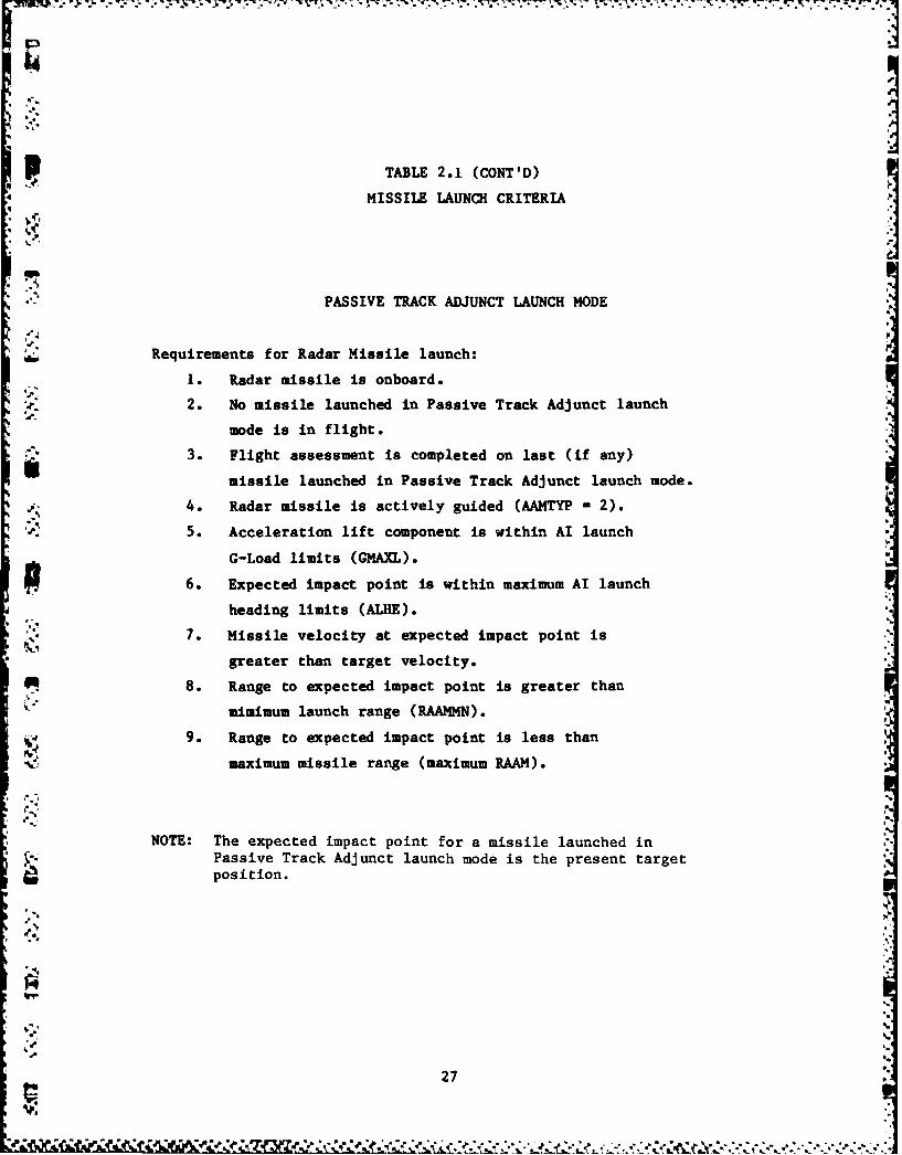
TABLE 2.1 (CONT'D)

4MISSILE LAUNCH CRITERIA

PASSIVE TRACK ADJUNCT LAUNCH MODE

Requirements for Radar Missile launch:

1. Radar missile is onboard.

2. No missile launched in Passive Track Adjunct launch

mode is in flight.

' 3. Flight assessment Is completed on last (if any)

missile launched in Passive Track Adjunct launch mode.

4. Radar missile is actively guided (AAMTYP - 2).

5. Acceleration lift component is within AI launch

G-Load limits (GMAXL).

6. Expected impact point is within maximum AI launch

heading limits (ALHE).

7. Missile velocity at expected impact point is

greater than target velocity.

8. Range to expected impact point is greater than

t mimimum launch range (RAAMMN).

9. Range to expected impact point is less than

maximum missile range (maximum RAAM).

NOTE: The expected impact point for a missile launched inPassive Track Adjunct launch mode is the present targetposition.

27-

t' ,, 'i ; .e,"eir," '. , .*'e < '.e "'.'. .r.";'. '€;'o "" " "",' '\''.'.,'' " '.' ''. 27"...

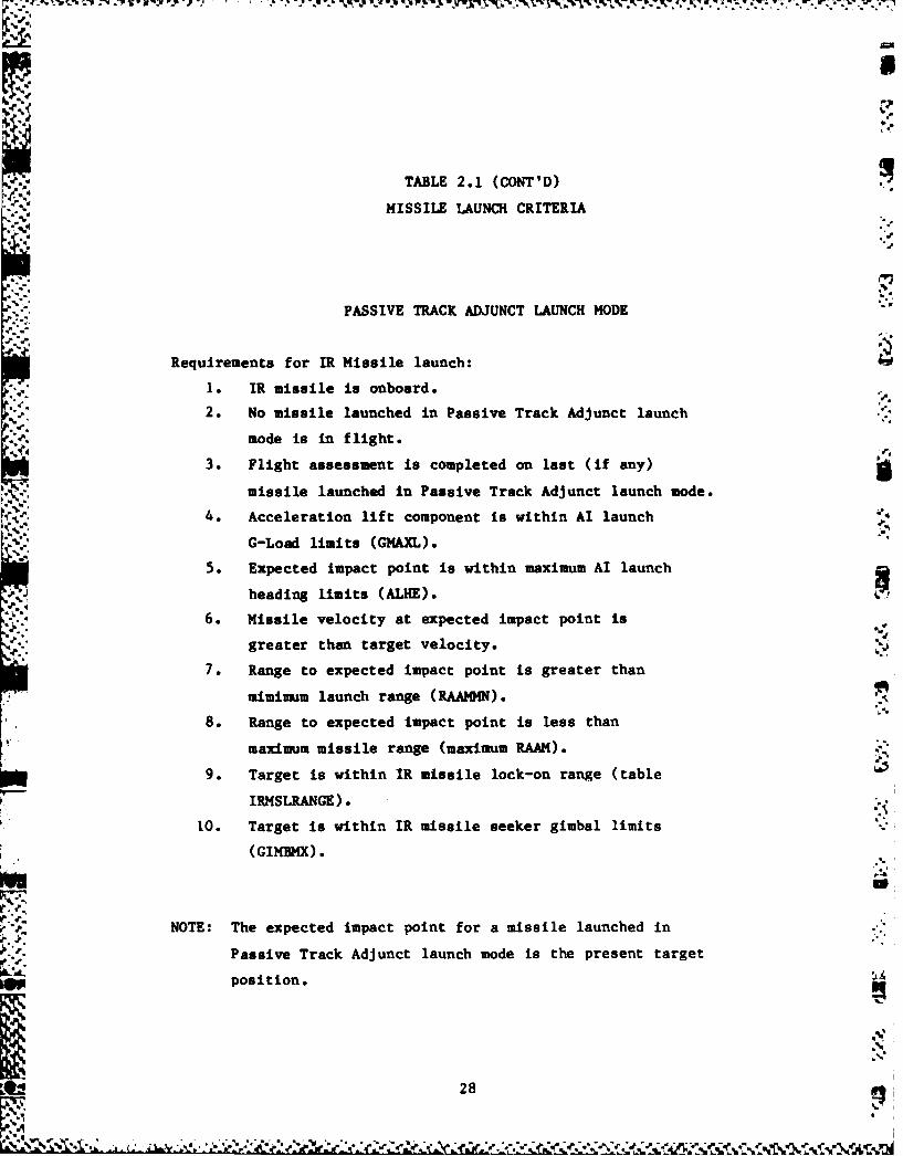
TABLE 2.1 (CONT'D)

MISSILE LAUNCH CRITERIA

PASSIVE TRACK ADJUNCT LAUNCH MODE

Requirements for IR Missile launch:

• • 1. IR missile is onboard.

2. No missile launched in Passive Track Adjunct launch

mode is in f light.

3. Flight assessment is completed on last (if any)

missile launched in Passive Track Adjunct launch mode.

4. Acceleration lift component is within AI launch

G-Lod limits (GMAXL).

5. Expected impact point is within maximum AI launch

heading limits (ALHE).

6. Missile velocity at expected impact point is

greater than target velocity. "-y

7. Range to expected impact point is greater than

mimimum launch range (RAANMN).

8. Range to expected impact point is less than

maximum missile range (maximum RAAM).

9. Target is within IR missile lock-on range (table

IRMSLRANGE).

10. Target is within IR missile seeker gimbal limits

(GIMBMX).

NOTE: The expected impact point for a missile launched in

Passive Track Adjunct launch mode is the present target

position.

28

TABLE 2.1 (CONT'D)Zj

MISSILE LAUNCH CRITERIA

RADAR TRACK LAUNCH MODE

Requirements for Radar Missile launch:

1. Radar missile is onboard.

2. No missile launched in Radar Track launch

mode is in flight.

3. Flight assessment is completed on last (if any)

missile launched in Radar Track launch mode.

4. Acceleration lift component is within Al launch

G-Load limits (GMAXL).

5. Expected impact point is within maximum AI launch

qheading limits (ALHE).6. Missile velocity at expected impact point is

greater than target velocity.

7. Range to expected impact point is greater than

Pmimimum launch range (RAAMMN).

" 8. Range to expected impact point is less than

maximum missile range (maximum RAAM).

9. Signal-to-Interference ratio (S/I) is above threshold

* (SIRAAM) for semi-actively guided radar missile type

(AAMTYP - 1).

10. Target is within missile seeker gimbal limits (GIMBMX)

for semi-actively guided radar missile type.

'a. NOTE: The expected impact point for a missile launched in Radar Track

launch mode is a lead pursuit aim point based on a non-

maneuvering, constant-velocity target.

29 !

-e.

• o i.

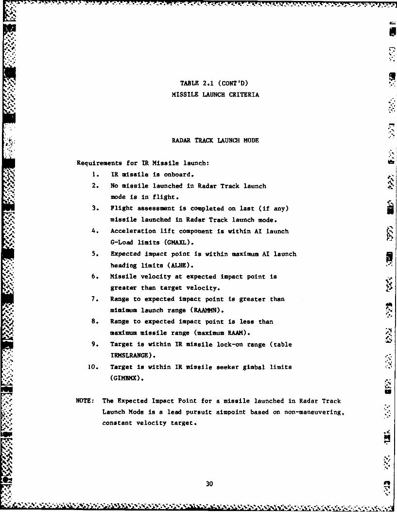
TABLE 2.1 (CONT'D)

MISSILE LAUNCH CRITERIA

RADAR TRACK LAUNCH MODE

Requirements for IR Missile launch:

1. IR missile is onboard.

2. No missile launched in Radar Track launch

mode is in flight.

3. Flight assessment is completed on last (if any)

missile launched in Radar Track launch mode.

4. Acceleration lift component is within AI launch

4 G-Load limits (GMAXL).

5. Expected impact point is within maximum AI launch

" heading limits (ALHE).

6. Missile velocity at expected impact point is

greater than target velocity.

7. Range to expected impact point is greater than

mimimum launch range (RAAMMN).

8. Range to expected impact point is less than

maximum missile range (maximum RAAM).

9. Target is within IR missile lock-on range (table

IRMSLRANGE).

10. Target is within IR missile seeker gimbal limits

(GIMBMX).

NOTE: The Expected Impact Point for a missile launched in Radar Track

Launch Mode is a lead pursuit aimpoint based on non-maneuvering,

constant velocity target.

30 W

Lz:-!

.F

The target, AI, and missile flight models are all three-degree-

of-freedom models, and are described in Appendices D, E, and F. The

,> guidance for the target is provided by the user, as a series of

maneuvers. The guidance for the AI is dynamically determined at each

4.f" ~time step based on a new maneuver aim point. The type of guidance for

the missile is selected by the user.

2.4.4 The Attack Phase

t In the ENGAGE II simulation, the interceptor aircraft continues

Sthe engagement until an end condition is encountered. Until then, the

pilot launches missiles when he can, following a shoot-look-shoot

bphilosophy. The user inputs a value for the time delay between the

impact of one missile and the launch of the next missile (TSMI2L). This

* ".. time delay accounts for attack assessment, trigger squeeze, and missile

launch. ENGAGE II limits the number of missiles (these could also be

considered salvos) with inputs by the user (AAMNUM(RADMIS) and

" (AAMNUM(IMIS)).

After the launch of a missile, the simulation continues to monitor

the flight of the missile for any type of failure, as well as to check

for the closest approach. There are three general causes for in-flight

missile failures.

. The missile flight exceeds the maximum guided flight

' -, time (TDMAX).

The missile blind flight exceeds the maximum blind flight

.4 time (TDIIN).

• The missile flies below ground level.

*4g3

-02PROP7 .7 01k T -7 7-3- .7 .,

Conditions which cause blind flight are similar to those which inhibit

launch. These depend on the missile launch mode at the time the missile

was launched. A list of conditions which must be met for guided

(non-blind) flight are given in Table 2.2. When these conditions are

not met, the flight is temporarily blinded. If it continues beyond an

input maximum blind flight time (TDMIN), the flight must abort. For

instance, if the missile is a semi-actively guided radar missile, the AI

radar must continue to illuminate the target by keeping it within the AI

radar gimbal limits. If the illumination fails, the missile flies blind

for a specified time, then aborts. If the target illumination by the AI

radar is reestablished before the maximum blind flight time, the missile

flight continues. If the radar missile has an active seeker, the seeker

need rt detect and lock-on to the target until a user-specified time

(TSAACQ) before the expected impact.

Missile flight assessment takes place after the missile has

reached its closest approach to the target. This closest approach is

defined as the first time the range rate between the missile and the

target is zero or positive. The missile model integrates to provide the

time (within 0.00001 seconds) when this happens; the range between the 791

missile and the target at this time is called the miss distance. The

user can add an aspect-dependent error to the miss distance (tables

IRMISSERR and RADMISSERR). The resultant miss distance is then used to

calculate the missile probability of kill, PKSS,

PKSS - 1 - 0.5(RLETHL/MISDIS)2

U

% where RLETHL is the lethal radius of the target for this missile

type (the radius with PK - 0.5); and MISDIS is the missile miss

distance, including any user added error.

32 '-

bklw E -x L .V kmg% N.5'

I .4

TABLE 2.2

MISSILE GUIDED - FLIGHT CRITERIA

Il.

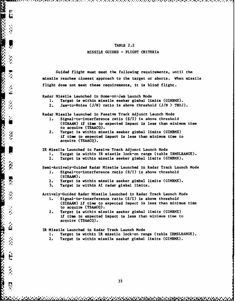
Guided flight must meet the following requirements, until the

'4 missile reaches closest approach to the target or aborts. When missile

flight does not meet these requirements, it is blind flight.

Radar Missile Launched in Home-on-Jam Launch Mode1. Target is within missile seeker gimbal limits (GIMBMX).2. Jam-to-Noise (J/N) ratio is above threshold (J/N > THOJ).

Radar Missile Launched in Passive Track Adjunct Launch Mode

1. Signal-to-interference ratio (S/I) is above threshold(SIRAAM) if time to expected impact is less than minimum timeto acquire (TSAACQ).

. *-, 2. Target is within missile seeker gimbal limits (GIMBMX)," if time to expected impact is less than minimum time to

acquire (TSAACQ).

IR Missile Launched in Passive Track Adjunct Launch Mode1. Target is within IR missile lock-on range (table IRMSLRANGE).2. Target is within missile seeker gimbal limits (GIMBMX).

Semi-Actively-Guided Radar Missile Launched in Radar Track Launch Mode

1 1. Signal-to-interference ratio (S/I) is above threshold(si5AM).

, 2. Target is within missile seeker gimbal limits (GIMBMX).Ie 3. Target is within AI radar gimbal limits.

S" Actively-Guided Radar Missile Launched in Radar Track Launch Mode1. Signal-to-interference ratio (S/I) is above threshold

(SIRAAM) if time to expected impact is less than minimum time2. :to acquire (TSAACQ).

.. 2. Target is within missile seeker gimbal limits (GIMBMX)if time to expected impact is less than minimum time to

" -. acquire (TSAACQ).

IR Missile Launched in Radar Track Launch Mode1. Target is within IR missile lock-on range (table IRMSLRANGE).2. Target is within missile seeker gimbal limits (GIMBMX).

..-,

5 33

%N°

The probability of kill for the engagement, PK, is then

.-J

NMIS

PI -1- (I- PKSS)

i-I

where NMIS is the number of missiles launched during the engagement.

During the course of the attack phase, the target doppler may

enter the region of the mainlobe clutter filter where the AI radar -.

cannot track. The target may maneuver in a way which reduces the target

RCS so that the signal-to-interference ratio falls below the radar

threshold. In either of these cases, AI radar tracking may fail, and

the tracking gates of the AI radar then usually enter a coasting phase,

making use of its memory of the motion of the target. Various logic is

used in Al radars to enable the tracking filters to pick up the target

when it exits this clutter region. If the time is short, ENGAGE II

allows the AI to continue to maneuver, modeling the effect of tracking

memory. When the target exits this clutter region or the signal rises,

tracking is assumed to reinitiate immediately and steering commands are

imediately made available to the pilot. If, however, this coasting 4time is too long (TCOAST), then the AI radar must reacquire the target.

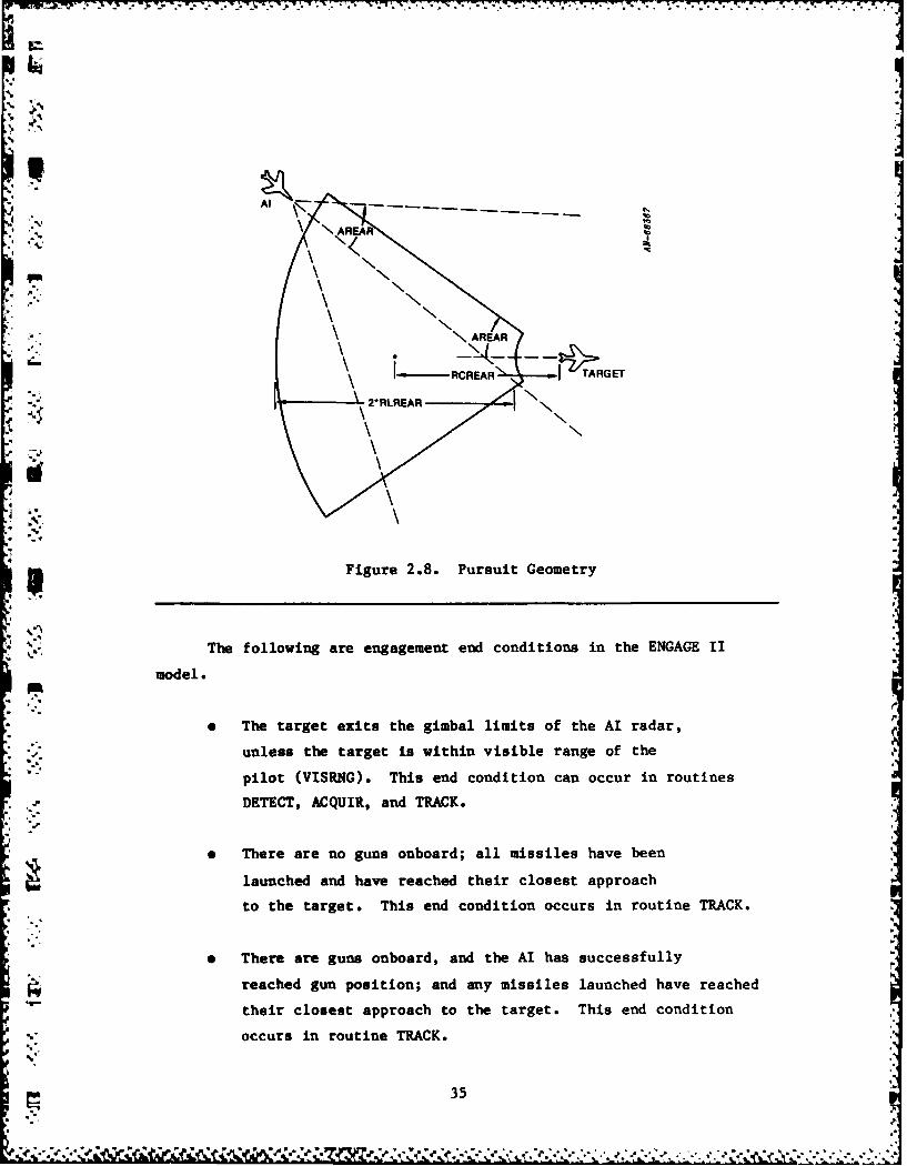
If guns are onboard, once the Al radar has locked-on and all

missiles are launched, the AI will attempt to reach a gun-firing

position. The area defining this position is illustrated in Fig 2.8. A

similar pursuit area for IR missile& is also defined by the user. These

areas are used by the model to help guide the AI to a stern attack.

The AI maneuvering model is described in Appendix D.

34

-i "-"" -. - ",:-" - - .. . . - , - . . - .- .., ., .. . ,t . , € ,

'101

'Al

-RCREAR 'TARGET

- :o \

S %°

4!

Figure 2.8. Pursuit Geometry

The following are engagement end conditions in the ENGAGE II

model.

* The target exits the gimbal limits of the AI radar,

. unless the target is within visible range of the

pilot (VISRNG). This end condition can occur in routines

DETECT, ACQUIR, and TRACK.

.4

0 There are no guns onboard; all missiles have been

launched and have reached their closest approach

to the target. This end condition occurs in routine TRACK.

* There are guns onboard, and the AI has successfully

4 reached gun position; and any missiles launched have reached

their closest approach to the target. This end condition

occurs in routine TRACK.

S %3

i: 35 "

-'

oN.1

0 The engagement time exceeds the maximum time (TABORT)

allowed for an AI engagement. This end condition can occur in

Sroutines DETECT, ACQUIR, and TRACK.

"" . The target is beyond 90 degrees off the boresight of

the AI heading, and the AI radar has not yet locked-on to the target. This end condition may occur in routines

DETECT and ACQUIR.

2.5 MODEL USES AND LIMITATIONS

The model uses a missile flight table, containing missile range

and velocity versus time, to determine when launch requirements have

been met and to calculate the lead aim point for the AI maneuvers.

There is a separate table for the radar missile and the IR missile.

These tables must be appropriate to the geometry being simulated (launch

velocity and altitude, target velocity and altitude). However, if these

parameters vary by large amounts within an engagement, missile aim

points and launch requirements may be incorrect, and launches may occur

too early or too late.

Since the model assumes that the engagement is initiated as the

result of GCI vectoring, the PD and PDC values are valid only when the

assumptions used to establish the GCI positioning (HCAs and offsets) are

valid. They would not be appropriate for "random" encounters, where the

AI has received no guidance from GCI.

There are three ECM techniques in the model. These are used

against the AI radar. Only the first, Noise Jamming, is modeled as

affecting the missile seeker and then only to allow home-on-jam missile

guidance. The others, Track Break and DECM, do not affect the radar

'P missile seeker.

36

% . - Missile flyout does not include any limitations other than time. lag, propulsion level, and aerodynamic maneuverability of the missile.

The user may simulate other errors which affect miss distance by using

the target-aspect-dependent miss distance error tables (tables IRMISSTAB

and RADMISSTAB).

The target can maneuver, but the aim points for the AI and

missiles are not based on predictions of target acceleration; they use

• -only target velocity.

The target maneuvers must be defined by the user before the

engagement is run; to simulate any reactive maneuver, the user must run

the engagement, decide on the time, magnitude, and direction of the

.. maneuver, and rerun the engagement with altered target maneuver input

directives.

Tactical options are rather rigid. For example, breakaway does

". . not commence until all radar missiles are fired, no matter how close the

:J: \ target is. The AI continues to fly a lead collision course as long as

there are missiles remaining. No attempt is made (until break away) to

* maintain stand-off from the target. The underlying assumption is that

the target cannot shoot back.

The missile is "guided" all the way to the target, even if it is a.

lock-on-after-launch radar missile. This means that during the period

between missile launch and seeker lock-on the missile flies according to

the chosen guidance mode (proportional, pursuit or tail-chase) rather

than using inertial or command guidance. These two guidance options

could be added, but would require addition of a more detailed simulation

of the Al fire control computer.

•: *,

."p- Missile launch decisions during PTA track assume that target speed .

but not direction is known. That is, no prediction of the target

position at intercept is made, but a check to see that the missile

velocity exceeds the target velocity is made.

The clutter is modeled using a backscatter coefficient of

y sin(6). This model is a reasonable approximation for clutter returns

over ground terrain, but is not appropriate over water. Entirely new

algorithms to calculate signal-to-clutter ratios would have to be

developed to treat sea clutter.

I!i.,.

'4

4% "38

3 ENGAGE II INPUT DESCRIPTION

This section describes the inputs for the program ENGAGE II. The

methods of setting the input data are described in Sec 3.1; the general

format of the data is given in Sec 3.2; and the input variables are

described in Sec 3.3. Default values are mentioned in Sec 3.4.

3.1 SOURCES OF INPUT DATA '

The input data may reside in one or several files, and may also be

keyed in interactively during a run. Reading inputs from any unit (an

*input file or the terminal*) ends with the 3-letter word "END". At

least one input file (unit 1) is expected, and terminal input (unit 5)

is required. (Either could be the single input "END".) During

interactive (unit 5) input, the user may indicate other input units

(other files) to read. To do so, the user types:

FILE - Lunit

where "Lunit" is the logical unit number for the program to read. The

1 program then reads from that logical unit until it encounters an "END",

and returns to interactive mode. The user may input more data, select

another input unit to read, or end the inputs and begin program

calculations.

If additional input files are needed, the user must make any necessary

file assignments before program execution.

For example:

The user has two input files for ENGAGE II. The f: is assigned as

the standard input file on unit 1. The second file, MORDAT, contains

additional input data. Before execution:

*The term "terminal" here refers to the primary input file. On anon-interactive system it may, in fact, be a card deck or disk file.

39

On the VAX: ASSIGN MORDAT.DAT FOR021

on the CDC: GET (TAPE21 - MORDAT)

After execution begins, unit 1 is read and then the user is prompted for

- input data. The user types:'p.

FILE - 21

The program will read MORDAT input data, then prompt the user for more

terminal inputs.

3.2 INPUT DATA FORMAT

The ENGAGE II input format is similar to FORTRAN NAMELIST, with

the basic form:,.

NAME " Value UNITS.4d

,'-" where:

NAME is the parameter name (See Sec. 3.3)

Value - is the value to be assigned (decimal point not required

for whole numbers)

and UNITS - name of units of input value4--

Blank spaces on each input line are ignored and may be used at will for

readability. UNITS is optional, and if not given will default to the ,.

appropriate unit in the English units system (feet, pounds, seconds,radians) which are the internal units used in the program. The list of

allowable UNITS names is given in Table 3.1 (page 69). The user may

indicate default units even though this will not affect the value, to-=

aid in documenting the data for later understanding.

40 .

".V.L":, .'," .. '", ', -lz ',' / ' ,. , .. .... :," '',"-,:, N ,, .,.,.''.. % ',,.'.. -.. ,-...;.."."-. . . . -- ,-.. ...- ,

SAn example is:

VI - 800 FPS

This will define the velocity of the Air Interceptor to be 800

ft/sec.

Some parameter names may be indexed by type. The form is then:

NAME (INDEX) - Value UNITS

where:

INDEX is the mneumonic identifier of the index of the parameter.

• .The possible indices are:

INDEX PARAMETER

RADMIS for the radar missile, and the radar missile seeker PRF

mode

IRMIS for the IR missile, and the IR missile pursuit area

AI for the Air Interceptor

.01 AI-HI for the High PRI mode of the AI

AI-MED for the Medium PRF mode of the AI

AI-LOW for the Low PRF mode of the AI

" GUNS for the Gun pursuit of the AI

For example, if there are 3 radar missiles on board the AI, and I IR

missile:

AAMNUM(RADMIS) - 3.

AAMNUM(IRMIS) - 1.

- * The input parameter descriptions in Sec. 3.3 indicate which, if any, of

the index values are valid.

41

t .

441

041

Some inputs are arrays. For these, a scalar input usually def ines the

number of elements in the array, and then the elements of the array are

assigned to the array name. For example:

-p..NHCA 4

HCA -0, 30 DEG, 150 DEG, 180 DEG

This will assign four Heading Crossing Angles, with values of 0, 30,

150, and 180 degrees. Note that DEG is used to define units different -

from the default, which is radians. A single value in the table can be

reassigned by referencing the proper index. For instance, the third

Heading Crossing Angle can be modified to 90 degr-tes for a subsequent

run.

HCA(3) - 90 DEG '.

Comments may be added to the input stream to help the user document the

data. Comments begin with a slash (/), and continue to the end of the

input line. For instance:

/These are the flight engagement parameters

4' NHCA - 1, HCA - 180 DEG /Head on case only

The first line is all comment; the second line contains input data

assignments followed by a comment. Note that more than one assignment -

may be made on the same line. '

3.3 INPUT~ DATA DESCRIPTION

3.3.1 ENGAGE II Run Parametersb

0 RUN OPTIONS

These options control the type of output generated by a programrun.

42 o

I.'..

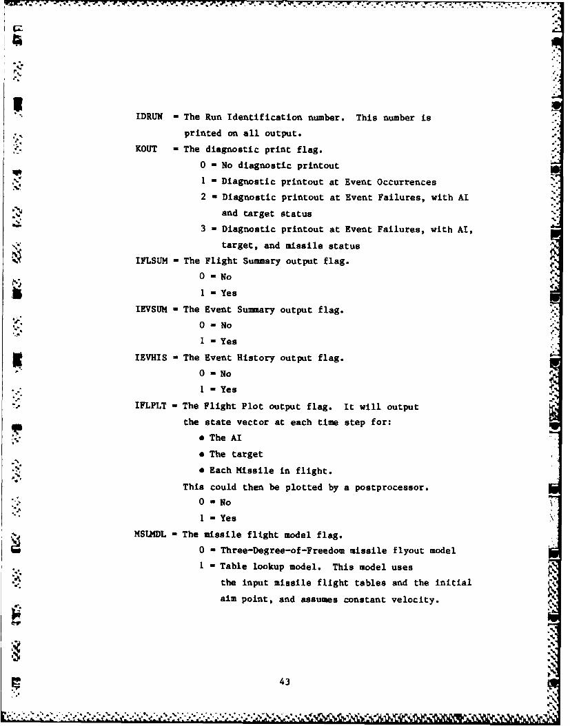
" IDRUN - The Run Identification number. This number is

printed on all output.

KOUT = The diagnostic print flag.

0 - No diagnostic printout

1 Diagnostic printout at Event Occurrences.

2 - Diagnostic printout at Event Failures, with AIand target status

3 - Diagnostic printout at Event Failures, with AI,

target, and missile status

IFLSUM = The Flight Summary output flag.

0-No

1 - Yes

IEVSUM - The Event Summary output flag.

0 -No

I - Yes

IEVHIS - The Event History output flag.

0 -No

I Yes"¢-.*

IFLPLT = The Flight Plot output flag. It will output

the state vector at each time step for:

,. * The AI

* The target0 Each Missile in flight.

This could then be plotted by a postprocessor.

0 - No

I - Yes

MSLMDL = The missile flight model flag.

0 - Three-Degree-of-Freedom missile flyout model

1 - Table lookup model. This model uses

the input missile flight tables and the initial

aim point, and assumes constant velocity.

43

"* * * % ., *.. % * . . . . . . . * . am~

FLIGHT CASE GEOMETRIES SELECTIONThese parameters define the number of engagements in the run, and

describe the vectoring instructions and errors for each of these

engagements. These parameters are illustrated in Fig. 2.3.

NHCA - The number of different Heading Crossing Angles

to generate engagements. The maximum allowed is 7.

NOFF - The number of different offset distances for each

Heading Crossing Angle. The maximum allowed is 11.

NOFF is reset to the maximum allowed if the offset

distribution flag, IOFDIS, is 0 or I (uniform

or normal distribution.)

IOFDIS - The offset distribution flag. This flag defines

how the different offset distances are determined.

0 - Uniform distribution for 11 offsets.

Maximum offset is OFF(1) value.

1 - Normal distribution for 11 offsets.

One sigma offset is OFF(1) value.

2 - User input offset distribution.

DLAG - The distance behind the target to which vectoring is

desired.

RIO - The range at which the engagement begins (the vectored

AI turns on the radar) when the Heading Crossing

Angle is 0. degrees, the Tail chase geometry.

RIPI -The range at which the engagement begins (the vectored

AI turns on the radar) when the heading crossing

angle is 180. degrees, the Head-on geometry.

The range for intermediate heading crossing angles

is calculated using linear interpolation between

RIO and RIPI.

TABORT - The maximum AI flight time for a single engagement.

HCA(I) - Heading crossing angles for I-1 to NHCA.

OFF(J) - Offset distances from J-1 to NOFF

44

-44 9

AIR INTERCEPTOR GEOMETRY

The following parameters describe the flight and maneuverability

"N of the AI.

ACCHAX The maximum acceleration of the AI in level flight.

4, This is used to limit any requested velocity change

for the AI.

ALTINT - The altitude of the AI at the beginning of the

engagement.

DCCMAX - The maximum deceleration of the AI in level flight.

This is used to limit any requested velocity change

for the AI.

GLOAD - The maximum gravity force load of the AI.

GUNS = The Combat guns flag. If this flag is set to I,the AI will attempt to maneuver to a successful

gun-firing position after all missiles have been

launched.

0 - No guns

I - Combat guns on board - try for gun position

PRIOML - Missile launch priority. This flag determines which L

type of missile to attempt to launch first, at any

given time, and may affect the AI maneuvering

if IR missiles have launch priority and they are

aspect dependent.

I - Launch radar missiles before IR missiles

*" if possible

2 - Launch IR missiles before radar missiles

if possible

RRMAX - AI roll rate limit. If a maneuver is requested which

requires a roll greater than RRMAX in the next time

.". step, then the maneuver will not begin until enough -

time has passed for the full roll requested.

45

TSMI2L - The minimum time between one missile intercept

(closest approach or missile abort) and the next

missile launch. This is the time required for

kill assessment. This time period is required for2' successive missiles launched in the same mode. It is

not required between two missiles launched in different

modes, such as one missile launched in Passive Track

Adjunct Launch mode and another launched in Radar Track

Launch mode. This is also the time period required

between the beginning of radar track and the first radar

track missile launch.

VI - The velocity of the AI at the beginning of the

engagement.

VIMAX - The maximum allowed AI velocity.

VIMIN - The minimum allowed AI velocity.

VISRNG - The visual range of the pilot of the AI. This is

not aspect dependent. It is used in Track mode to

override the radar in close range, so the engagement

does not end if the target is outside the radar

gimbal limits. When the target is within the visualrange of the AI, deceptive ECM does not perturb the AI's

knowledge of the target position.

* PURSUIT DIRECTIVES

The rear area of pursuit is the region behind the target

illustrated in Figure 2.8. The rear area of pursuit may be

defined by index for guns, using index "GUNS"; and for IR

missiles, with index "IRMIS". The "GUNS" area designatessuccessful gun position for guns, and the "IRMIS" area provides %

an aimpoint for AI maneuvers for rear-aspect-dependent IR missile

launches. (The following parameters are indexed. The index is

"GUNS" for gun pursuit directives, and "IRMIS" for IR missile

pursuit directives).

46 I

AREAR The half angle of rear area pursuit. This

,.?' angle, measured from the tail of the

target, is the maximum angle of the AI

off direct tail pursuit of the target.The same angle is the maximum allowed

for the target off the nose of the AI.

RCREAR - The range to the center of the rear area

of pursuit, behind the target.

RLREAR - The half-length of the region of the rear area

of pursuit.

TSREAR - The time step for terminal approach for the

rear area of pursuit. This time step is used by the

'S model whenever the AI is within the effective pursuit

radius of the target, no matter what the angle is. The

effective pursuit radius is RCREAR+RLREAR.

0 PASSIVE TRACK ADJUNCT PARAMETERS

The parameters describe the Passive Track Adjunct onboard the AI.

PAZGMB - Passive Track Adjunct azimuth gimbal limit. Gimbal

* limits are used in the PTA autonomous mode, once-detection has occurred.

PELGMB - Passive Track Adjunct elevation gimbal limit.

PAZSCN - Passive Track Adjunct azimuth scan limit. Scan limits

are used in the PTA detection process.

PELSCN - Passive Track Adjunct elevation scan limit.

PTAFLG - Passive Track Adjunct mode flag.

0 - No Passive Track Adjunct.

-1 - Radar clue mode. In this mode, the radar scan

"" time is redefined after successful PTA.

47

.* L%. S%-. ** *

-~T- - 7- -

2- Autonomous mode. In this mode, once detection

has occurred, both radar and IR missile launch

attempts may be made, and the AI may maneuver

toward the target.

TSPTA - Passive Track Adjunct scan time step.

TSTA2R - New radar scan time step for radar detection

after Passive Track Adjunct detection is successful. T

The radar scan time is modified only when

the Passive Track Adjunct is in radar clue mode (PTAFLG

- 1). This accounts for a smaller radar scan area, , "

defined by the PTA information on target location.

TSTARE - The time step between the first successful

Passive Track Adjunct return and a reasonable

range estimate. A missile cannot be launched

in PTA launch mode until this time period is

past. This input is only used when the Passive

Track Adjunct is in autonomous mode (PTAFLG - 2).

AI ANTENNAP2,

The following parameters describe the antenna of the AI radar.

These define the radar scan time and angular limits of the scan.

These antenna parameters are used to calculate the AI radar scan

period, which is used when the detection criterion is based on

cumulative PD (IDETYP - 2).

AZRATE - The AI radar azimuth scan rate

AZSCAN - The AI radar azimuth scan half-angle. The radar scans

from minus to plus this value.

BARSEP - The elevation bar separation angle of the Al radar.

ELBARS - The number of elevation bars in an AI radar scan.

ELCTR - The center angle of the elevation scan of the AI radar. I:44

48 OW,

9-4

ATSHIFT - The time to shift bars in the Al radar scan.

These antenna parameters are used to calculate the

AI radar scan period, which is used when the

detection criterion is cumulative PD (IDETYP - 2).

* AI RADAR DETECTION CRITERION

These parameters describe the Al radar detection and define the

time steps used for the radar model.

DCRIT - AI radar detection criterion threshold. This is

either:

the threshold for single scan detection if IDETYP

or the threshold for cumulative detection if

IDETYP - 2

ACRIT = AI radar acquisition criterion threshold for

the signal-to-interference ratio. This threshold

9must be exceeded to initiate and continue

Al radar track acquisition and AI radar track.

TSDET = The detection time step for single scan detection.

(IDETYP - 1). Cumulative scan detection (IDETYP = 2)

uses the calculated AI radar scan period.

TSD2AC = The time step between radar detection and track

acquisition. This allows for the mechanical

switching required by the AI radar to switch from

scan mode to track mode.

TSACQ The AI radar track acquisition time step.

TSTRK = The AI radar track time step.

TCOAST = The maximum coast time allowed in radar track.

This is the maximum time the signal processor can

update the track filter without new data. After

this time, the radar must reacquire the target.

49

* ... .*i ' *m*. .w

IDETYP = The detection type flag. This flag determines the

method the radar uses to determine successful

detection of the target.

I - Detect on single scan Probability of Detection (K

blips of M scans).

2 = Detect on cumulative Probability of Detection.

KBLIP - The number of successful single returns

required in M scans for detection. This input

is only used for single scan detection (IDETYP - 1).

MSCAN - The maximum number of scans allowed to get

K blips for successful detection.

The maximum allowed is 11. This input is

only used for single scan detection (IDETYP 1).

AI RADAR

These are general AI Radar parameters.

GIMBAZ - The radar azimuth gimbal limit.

GIIMBEL - The radar elevation gimbal limit.

PFA - The probability of false alarm.

RSCOPE - The scope-limited range of the radar. This

hard limit requires the Al-to-target range

to be within RSCOPE for any possible radar

return.

TJEFF - The Jammer effectiveness threshold. This input

is only used if the target is in the track-break

jamming mode (TJAM - 2) or Deceptive ECM jamming mode

(TJAM = 3).

TOJ - AI radar Track-On-Jam flag.

i0 No Track-On-Jam capability.

I - Track-On-Jam capability onboard AI radar.

50

116

I TTOJ = The Track-On-Jam threshold. This input is only

used if the radar has Track-On-Jam capability

(TOJ - 1). The Jam-to-noise ratio must be above this

threshold for the AI Radar to detect in track-on-jam

mode.

VCHIN - The half-width of the altitude clutter filter.

Go VTHMIN - The half-width of the mainbeam clutter filter~for high PRF.

VTMMIN - The half-width of the mainbeam clutter filter

for medium PRF.

• AI RADAR AND SEEKER PERFORMANCE PARAMETERS

The following parameters are general radar parameters for both

1- the Al Radar and the Radar Missile Seeker. These parameters are

indexed. The index is "AI" for the AI radar, and "RADMIS" for

0 the missile seeker.

ALAMB - The radar wavelength.

AVGPWR - The average transmitter power times the

duty factor.

TGML - The transmitter mainlobe gain above isotropic.

RGML - The receiver mainlobe gain above isotropic.

* .' RGBL - The receiver backlobe gain above isotropic.

TBhMW - The transmit mainlobe beamwidth at the 3 DB

. point.

. RBMW - The receive mainlobe beamwidth at the 3 DB

point.

SIGMAX - The signal at the antenna face causing gain

compression.

FNOISE - The receiver noise factor referenced to input.

GAMMA - The ground backscatter coefficient for this

scenario.

ALOSSJ - The input loss at the receiver for a jamming signal.

51

.77

AI RADAR AND SEEKER PRF PERFORMANCE PARAMETERS

The following parameters are dependent on the PRF type. The AI

radar can have any combination of three PRF types: high, medium,

and low. The missile seeker is assumed to have only a single PRF

type, high. These parameters are indexed. The index is:

AI-HI for the high PRF type of the Al radar;

AI-MED for the medium PRF type of the AI radar;

* AI-LOW for the low PRF type of the Al radar;

or RADMIS for the high PRF type of the missile seeker.

PRFTYP - The PRF type availability flag. This flag

enables or disables a particular PRF type.

0-Disable this PRF type.

1 = Enable this PRF type.

RZERO - The range at which the target is detected

under free space conditions, when the target

RCS value is SIGMAO.

SNZERO - The Signal-to-Noise ratio at which the detection at

range RZERO occurs.

SIGMAO - The Radar Cross Section of the target for the given

RZERO and RI conditions.

RI - The range at which the target is detected

under conditions with in-band clutter, when

the target RCS value is SIGMAO.

GAMMAI - The ground backscatter coefficient for R1

conditions.

VII - The radar velocity for RI conditions.

ALTI - The radar altitude for RI conditions.

SCV - The sub-clutter visibility. This is the negative

of feedthrough.

TAU - The pulse length.

52

4 4

AAM SEEKER

These parameters describe the seeker on the radar missile.4-

AAMTYP = The missile seeker type flag.

1 - Lock on before launch (LOBL). This is

a semi-active missile type, requiring

AI illumination on the target during missile

flight.

2 " Lock on after launch (LOAL). This is

an active missile type, independent of

AI direction once it is launched.ACMBAAM - The half-width of the seeker mainbeam clutter

notch.

HOJ - The Seeker Home-On-Jam flag. Only radar missiles with

this capability can be launched during Track-on-Jam

launch mode.

0 - No Home-on-Jam capability.

I - Home-on-Jam capability available.

SIRAAM = The missile seeker threshold for the

signal-to-interference ratio.

THOJ - The Home-On-Jam threshold. This input is only

used if the seeker has Home-On-Jam capability

(HOJ - 1.). The Jam-on-Noise ratio at the missile

seeker must be greater than this threshold for guidance

, TSAAC for a Home-on-Jam launched missile.

TSAACQ The time step before expected impact for seeker

acquisition for an active (LOAL) type seeker.

.4

53

.4' , ]

- .~. d. . . .~ ** - ,I 4~. . . 4

1.7

0 AAM LAUNCH CRITERIA

These parameters describe the missiles onboard the AI.

(The following parameters are indexed. The index is "RADMIS"

for radar missiles, and "IRMIS" for IR missiles.)

AAMNUM - The initial number of missiles onboard.

The maximum is 20.

ALHE - The maximum allowed launch heading error.

GIMBMX - The gimbal limit of the missile. This angle is measured

from the velocity vector of the missile or of the AI

at launch time. The angle to the target must be within

this limit for guided flight.

GMAXL = The maximum gravity load of the AI at the

time of the missile launch.

RAAMKN - The minimum flight range of the missile for

effective guidance.

RLETHL - The lethal radius of this missile against

this target. This is the radius around the

target with PK-O.5; it is independent of

target aspect.

T1RMIN - The maximum time without guidance before

the missile will abort. This is the length

of time the missile tracking algorithms

can continue without new data.

TDhAX - The maximum guided flight time of the missile.

SMM FLIGHT TABLE

These missile flight tables are used to determine missile air

points for launch. These tables can be calculated using the

missile input data in Seca. 3.3.4 and 3.3.5 in utility program

AATEST. AATEST is described in Appendix H. (The following

parameters are indexed. The index is "RADMIS" for radar

missiles, and "IRMIS" for IR missiles).

54 -

AAMFTN - The number of entries in the AAM flight table.

The maximum number allowed is 25.

TDAAM - Time increment between flight table entries.

RAAM(I) - AAM flight table range I.

VAAM(I) - AA velocity at range RAAM(I).

The first entry in the

table is at missile launch, where RAM(1)=0.O

and VA(MM-()VI (the velocity of the AI).

* TARGET GEOMETRY

The following parameters describe the target, along with the

target-aspect-dependent tables.

ALTTGT - The altitude of the target at the beginning of

the engagement.

ASPDIR - IR aspect-dependency flag. This flag is used

to determine if it is better for the AI to

maneuver to a pursuit position to attempt

to launch IR missiles.

0 - Little or no aspect dependency (pursuit

maneuver not required)

1 - Large IR aspect dependency (indicates pursuit

as best maneuver)

BIASAZ - The bias error in azimuth. This input is only

used if the target uses deceptive jamming

(TJAM - 3)

BIASEL - The bias error in elevation. This input is only

used if the target uses deceptive jamming

(TJAM - 3)BIASR -The bias error in range. This input is only

used if the target uses deceptive jamming

(TJAM -3)

55

BWJAM - The jammer bandwidth. This input is only

used if the target has some jamming capability

(TJAM is greater than 0)

TJAM -The target jammer flag.

0 - No jamming

I - Noise Jamming (delays radar detection)

2 - Track break (delays radar acquisition)

3 - Deceptive ECM (bias errors affect radar track)

*, VT - The velocity of the target at the beginning

of the engagement.

3.3.2 Target Maneuver Inputs

The target maneuver input table is indicated by the table name,

MANEUVER; then each maneuver follows as a set of 5 parameters. The

table ends with the word END. The 5 parameters needed to describe a

maneuver are:

* The duration of the maneuver

(Default units are seconds)

* The direction of the maneuver

(Direction is defined as

0 deg is right

90 deg is down

180 deg is left

270 deg (-90 deg) is up)

(Default units are radians)

. The magnitude of the maneuver (velocity-vector turn-rate)

(Default units are radians/second)

The longitudinal acceleration during the maneuver :4

(Default units are feet/second/second)

* The bank angle (not actually used by current program)(Default units are radians)

56 i

Up to 30 maneuvers may be stored for the target. If the target

completes all maneuvers in the maneuver table, it begins again at the

beginning of the table.

The following example will fly the target along a straight path for the

duration of the engagement.

IC *ii MANEUVER

99999 SEC, 0 DEG, 0 DGPS, 0 FPSS, 0 DEG

$ ~ END

The following example will fly the target in a continual sinusoidal

path.

MANEUVER

10 SEC, 0 DEG, 9 DGPS, 0 FPSS, 0 DEG,

20 SEC, 180 DEG, 9 DGPS, 0 FPSS, 0 DEG,

10 SEC, 0 DEG, 9 DGPS, 0 FPSS, 0 DEG,

END

In this example, units were used on all values even though "SEC" and

-_ "FPSS" are not necessary.

-~3.3.3 Target Aspect Tables

All target aspect-dependent tables have the same format. Each

table is immediately preceded by a table heading card and ends with an

"END" card. The table heading card format is:

TABLENAME (UNITS)

~ C' where:

TABLENAME is the name of the aspect table

and UNITS is the name of the units of the data

_% in the table.

Allowable units names are given in Table 3.1 (page 69).

o57

Aspect table names are:

RCSTABLE Target Radar Cross Section (RCS) table

ERPTABLE Jammer ERP table

IRMSLRANGE IR missile lock-on range tableIRMISSERR IR Missile miss distance error term tableRADMISSERR Radar missile miss distance error term table

PTATABLE Passive Track Adjunct lock-on range table

For example:

PTATABLE (NMI)

This indicates that the Passive Track Adjunct lock-on range table

follows, and the table data will be in nautical miles.

The user provides table data for equally spaced azimuth values

along a single elevation angle, repeating if there are several elevation

angles. Azimuth is measured from the nose of the target, so 0 degrees

is in front of the target, 180 degrees is behind the target. Elevation

is defined as positive above the target, and negative below. The target

is assumed to be symmetrical in azimuth about 0 degrees.

The order of the data in the table is defined by the table

parameters for that table. The table data is grouped by elevation, then

within elevation, by azimuth. Table parameters define the number of

table values for a single elevation, and the number of different

elevation angles represented in the table. The table parameters follow

the table heading card. The table parameters are:a.

NAZ - Number of table values in azimuth per elevation cut

(These values are assumed to correspond to azimuth

angles from 0 to 180 degrees.)

58 U,

'S '' T '". ¢ , .,. ,,.;',; .. ,':'.'/ 'r"':: -' ;;.';''"?" ' '- "",::. .. ,

NEL - Number of elevation cuts

ELMIN - Minumum elevation angle (first EL cut)

' ELSTP - Angle increment between adjacent elevationcuts

TABLE - Table data

SCALE - Scaling factor for all table entries (Default is 1.0)

- Table data is stored by azimuth angle, then elevation cut.~TAB(M

(For AZ from 0 to 180 degrees for each EL cut)

I - I TO NAZ For Ist EL cut at EL - ELMIN

- NAZ+1 TO 2*NAZ For 2nd EL cut at EU4IN+ELSTP

- 2*NAZ+1 TO 3*NAZ

For 3rd EL cut at ELMIN+2*ELSTP

" (NEL-I)*NAZ+I TO NEL*NAZ

For NEL-TH EL cut at ELMIN+(NEL-I)*ELSTP

Table data ends with "END". The total number of entries in the table is

NEL*NAZ.

When all parameters have been provided, a final "END" corresponds to the

end of an aspect table.

Example: Sample RCS table, with data at every 45 deg in azimuth, and

at 3 different elevation angles, -10, 0, and 10 deg.

1 .' Input data is in DBSM.

,59

Ig

'.i

* p :,! ~;

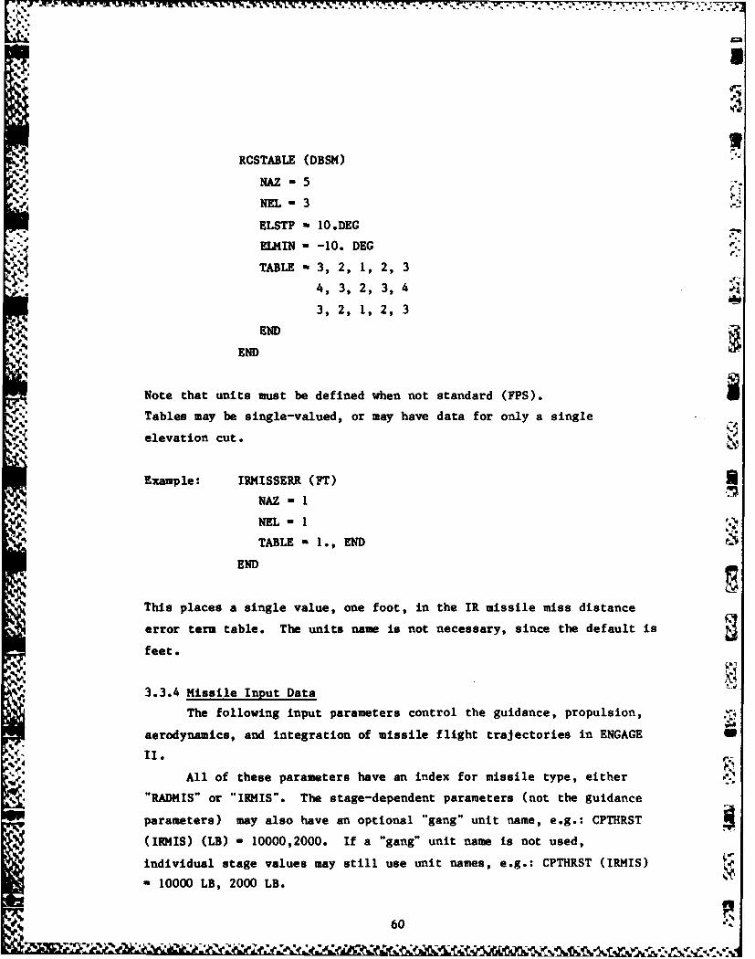
-*6

RCSTABLE (DBSM)

NAZ a5i L-3

ELSTP - 1O.DEG

ELMIN - -10. DEG

TABLE - 3, 2, 1, 2, 3

4, 3, 2, 3, 4

3, 2, 1, 2, 3

E END

Note that units must be defined when not standard (FPS).

Tables may be single-valued, or may have data for only a single

elevation cut. V

Example: IRMISSERR (FT)

NAZ -1

NEL- I

TABLE - 1., END

END

This places a single value, one foot, in the IR missile miss distance

error term table. The units name is not necessary, since the default is

feet.

3.3.4 Missile Input Data

The following input parameters control the guidance, propulsion,

aerodynamics, and integration of missile flight trajectories in ENGAGE

All of these parameters have an index for missile type, either

"RADMIS" or "IRMIS". The stage-dependent parameters (not the guidance

parameters) may also have an optional "gang" unit name, e.g.: CPTHRST

(IRMIS) (LB) - 10000,2000. If a "gang" unit name is not used,

individual stage values may still use unit names, e.g.: CPTHRST (IRMIS)

" 10000 LB, 2000 LB. M

60

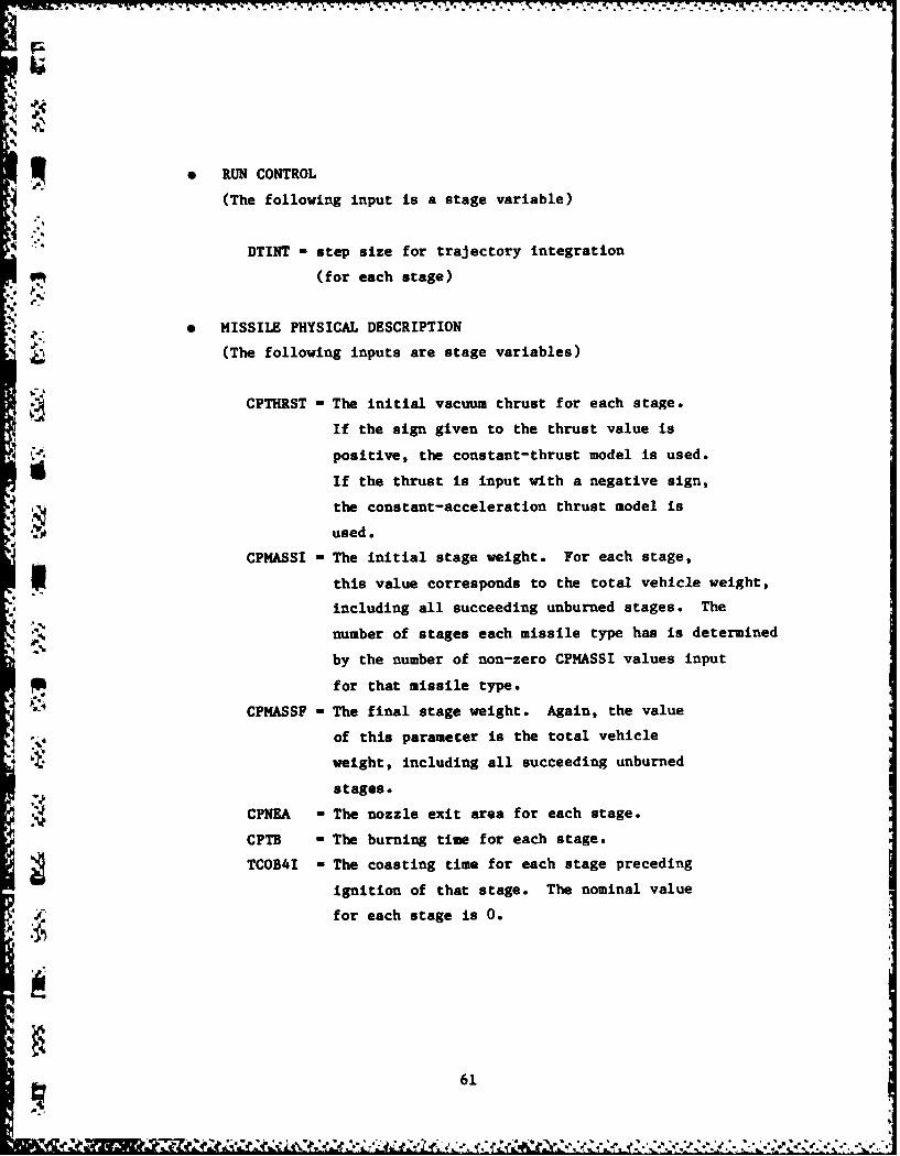
. RUN CONTROL

(The following input is a stage variable)

DTINT - step size for trajectory integration

(for each stage)

• * MISSILE PHYSICAL DESCRIPTION

(The following inputs are stage variables)

CPTHRST - The initial vacuum thrust for each stage.

If the sign given to the thrust value is

- positive, the constant-thrust model is used.

If the thrust is input with a negative sign,

the constant-acceleration thrust model is

used.

CPMASSI = The initial stage weight. For each stage,

U this value corresponds to the total vehicle weight,

*, including all succeeding unburned stages. The

number of stages each missile type has is determined

by the number of non-zero CPHASSI values input

for that missile type.

CPMASSF - The final stage weight. Again, the value

of this parameter is the total vehicle

weight, including all succeeding unburned

stages.

CPNEA = The nozzle exit area for each stage.

CPTB - The burning time for each stage.

TCOB4I = The coasting time for each stage preceding

ignition of that stage. The nominal value

4" for each stage is 0.

61

q Z c ~& *~~A

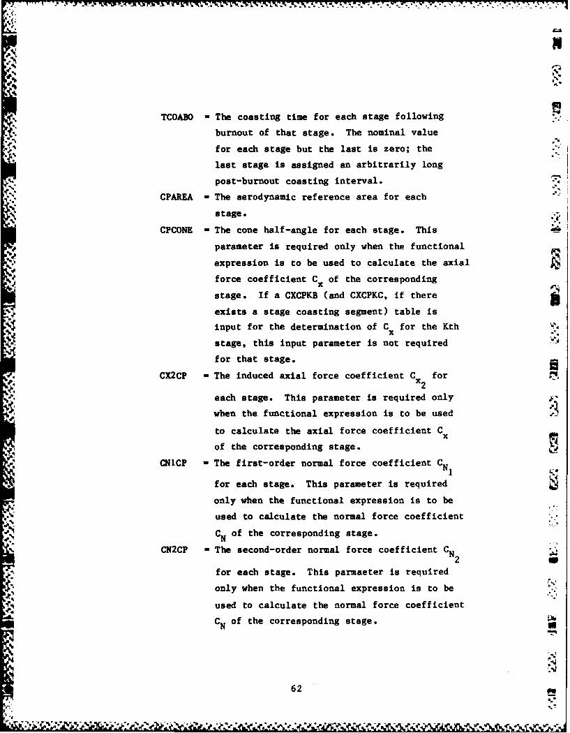
TCOABO = The coasting time for each stage following

burnout of that stage. The nominal value

, s for each stage but the last is zero; the

last stage is assigned an arbitrarily long

post-burnout coasting interval.

CPAREA - The aerodynamic reference area for each -

stage.

CPCONE - The cone half-angle for each stage. This

parameter is required only when the functional

expression is to be used to calculate the axial

force coefficient C1 of the corresponding

stage. If a CXCPKB (and CXCPKC, if there

exists a stage coasting segment) table is

input for the determination of Cx for the Kth

stage, this input parameter is not required

for that stage.

CX2CP - The induced axial force coefficient C forx2

each stage. This parameter is required only

when the functional expression is to be used

to calculate the axial force coefficient C

of the corresponding stage.

CNICP - The first-order normal force coefficient CN

for each stage. This parameter is required

only when the functional expression is to be

used to calculate the normal force coefficient

CN of the corresponding stage.

CN2CP =The second-order normal force coefficient CN

for each stage. This parmaeter is required

only when the functional expression is to be

used to calculate the normal force coefficient

CN of the corresponding stage.

NU

62

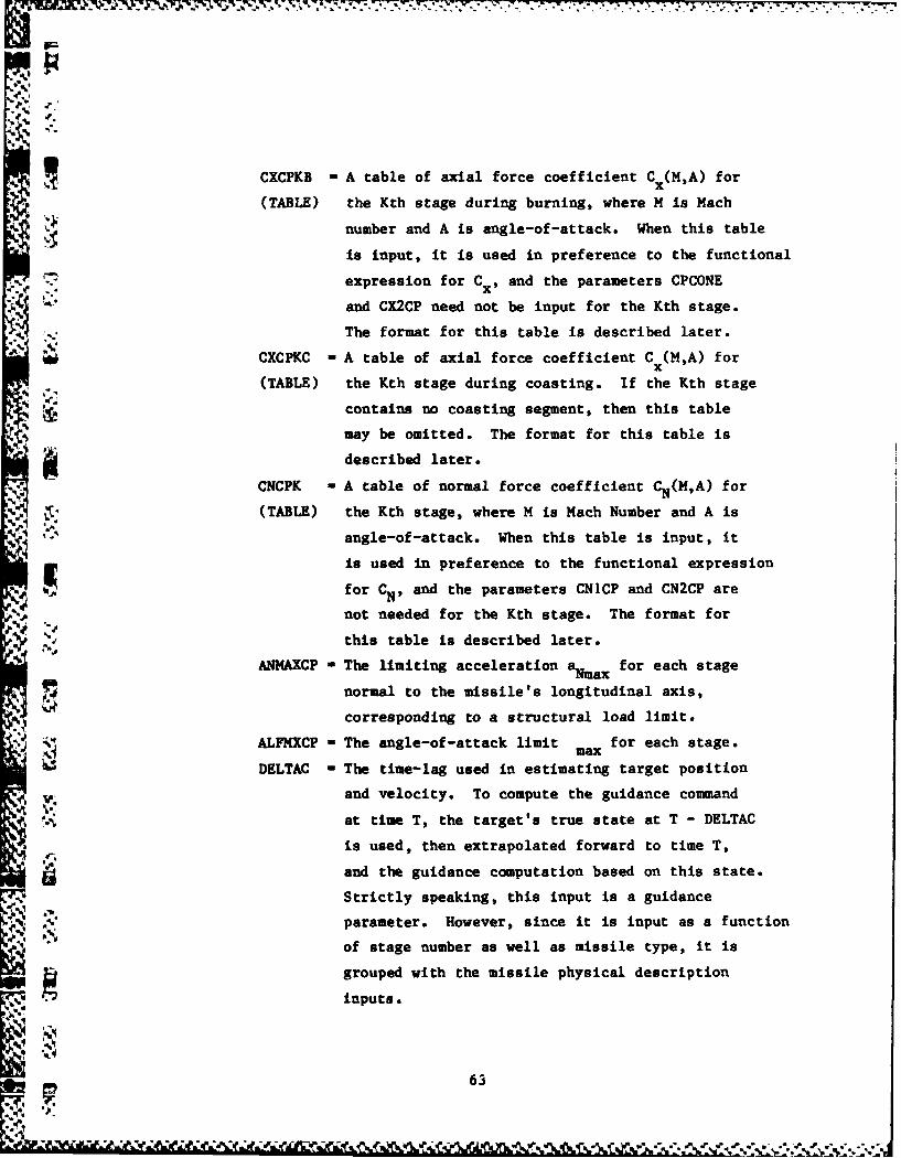
CXCPKB - A table of axial force coefficient C x(M,A) for

(TABLE) the Kth stage during burning, where M is Mach

number and A is angle-of-attack. When this table

is input, it is used in preference to the functional

expression for Cx , and the parameters CPCONE

and CX2CP need not be input for the Kth stage.

The format for this table is described later.

CXCPKC - A table of axial force coefficient C (M,A) for

(TABLE) the Kth stage during coasting. If the Kth stage

contains no coasting segment, then this table

may be omitted. The format for this table is

described later.

CNCPK - A table of normal force coefficient CN(M,A) for

(TABLE) the Kth stage, where M is Mach Number and A is

angle-of-attack. When this table is input, it

is used in preference to the functional expression

for CN , and the parameters CNICP and CN2CP are

not needed for the Kth stage. The format for

this table is described later.

ANMAXCP - The limiting acceleration aNmax for each stage

normal to the missile's longitudinal axis,

corresponding to a structural load limit.

ALFMXCP - The angle-of-attack limit max for each stage.

DELTAC - The time-lag used in estimating target position

. .v. and velocity. To compute the guidance command

at time T, the target's true state at T - DELTAC

'4 is used, then extrapolated forward to time T,

and the guidance computation based on this state.

Strictly speaking, this input is a guidance

parameter. However, since it is input as a function

of stage number as well as missile type, it is

grouped with the missile physical description

inputs.

63

IL

0 GUIDANCE PARAMETERS

GNAVI - The guidance gain for pursuit or proportional

guidance, minimum gain for tail-chase proportional

p. guidance

GNAV2 - The maximum guidance gain for tail-chase

proportional guidance.

ATANG - The tail-chase desired approach angle in tail-chase

Sproportional guidance.

.MAX - The maximum phantom target offset in tail-chase

proportional guidance.

AMIN - The minimum phantom target offset in tail-chase 3proportional guidance.

,GYE R - The guidance model selector.

o - pursuit guidance

I proportional guidance

2 - tail-chase guidance

INCLG = Guidance gravity flag. If zero, the guidance

command is satisfied using aerodynamic/thrust forces

only (gravity acts as a perturbation). If positive,

gravity is included vectorially in satisfying the

guidance command.

3.3.5 Missile Aerodynamic Table Input Format

Each table is immediately preceded by a table heading card. The

format is as follows:

TABLENAME (INDEX) (UNITS) where:

TABLENAME is the name of the table

INDEX is the missile index.

9..

64 ,

-L -9

and UNITS is the name of the units of the angle-of-attack

data in the table. Allowable units names

are given in Table 3.1 (page 69). The default,

if UNITS is not given, is radians.

The table names are:

------- Missile--------------------

Stage 1 Stage 2 Stage n (n - 3 to 7)

_ Cx during thrusting CXCPIB CXCP2B CXCPnB

C during coasting CXCPIC CXCP2C CXCPnCx

- CN CNCPl CNCP2 CNCPn

The missile index values are:

RADMIS Radar Missile

IRMIS IR Missile

The data to be tabulated for aerodynamic tables is:

1. Dimensionless Mach number (M)

2. Augle of attack (A) (UNITS, if given, refer to this data)

3. Dimensionless aerodynamic coefficient (C)

% The data should appear in the following order:

Ml, All, Cl1, A12, C12, .... Alnl, Clnl, END

M2, A21, C21, A22, C22, ..... A2n2, C2n2, END

Mr, Arl, Crl, Ar2, Cr2, .... Arnr, Crnr, END, END

where:

r is the number of Mach values in the table,

and n is the number of A,C pairs for each Mach kralue.

65

---------- .. .. . . .. . ._

'p.

Both Mach number and Angle-of-Attack entries must be arranged in .- *

monotonically increasing order. The word END signals the end of data

for a particular Mach value, with another END signifying the end of the

table. The program uses linear interpolation between adjacent values of

Mach number, while parabolic interpolation is used in angle-of-attack,

requiring at least three A,C pairs for each value of M. The number of

A,C pairs associated with each M need not be constant, nor need the ;

values of the A entries be identical for different values of M.

Extrapolation will be used if, during execution, the table is searched

with values for the independent variable M or A that range beyond the

values included in the table. For best accuracy, however, the tabulated

entries should encompass the entire expected range of values of these

variables. ott

The total length of all input aerodynamic tables combined may not exceed

800 values.

Example:

CXCP1B (IRMIS) (DEG)

1.25, 0.,.9, 3.,1.1, 6.,1.7, 12.5,4.0, END

1.75, 0.,.9, 3.,1.1, 6.,1.6, 12.,3.7, END

2.00, 0.'.8, 3.,1.0, 6.,1.5, 12.5,3.5. END

3.00, 0.,*8, 3.5,.9, 7.,1.3, 14.0,3.0, dND

4.00 0.,.7, 3.8,.8, 7.5,1.2, 15.0,2.5, END

END .4

3.4 INPUT VALUE DEFAULTS

The program has stored default values for all input variables.

The default value for all ENGAGE II Run Parameters (Sec 3.3.1) is zero,

except for two run options, IEVHIS and IFLSUM:

IEVHIS - I

IFLSUM - I

66

C~~~~~4 I .AI&ON W '

°.

Each target aspect table (Sec 3.3.3) is a single-valued table with

a single default value. These defaults are:

RCS Table: RCSTABLE - 1.

ERP Table: ERPTABLE - 1.

IR Missile Lock-On Range: IRMSLRANGE - 0.

IR Missile Miss Distance Error: IRMISSERR - 0.

Radar Missile Miss Distance Error: RADMISSERR - 0.

Passive Track Adjunct Lock-On Range: PTATABLE - 0. ..

The missile input data (Sec. 3.3.4) defaults are zero, with the

following exceptions:

GNAVI - 2

GNAV2 - 8

ATANG - 30 DEG

R1AX- 30 NMI

RMIN - 2 NMI

"; CPTHRST(1) - 5000

CPMASS1(1) - 1000

CPMASSF(O) - 500

CPNEA(1) I

CPTB() I .

TCOABO(1) - 99999

CPAREA(1) - 5

CPCONE(1) 1 10 DEG

CX2CP(1) = 0.0002 DG-2

CN1CP(1) - 0.05 DG-1

CN2CP(1) - 0.001 DG-2

ell* ANMAXCP(1) - 50 G

ALFMXCP(l) - 15 DEG

DELTAC(1) = 0.1DTINT(I-7) - 0.25

67,1

..

~These defaults hold for both RADMIS and IRMIS missile types. The

default condition for the missile aerodynamic tables (Sec. 3.3.5) is

null, i.e., no tables present."

.44

C8 '

-'I . ",- .. ,, . "% • • . - °m . - - • , - , % % - ., • •.. . . . . . - ,.. . -]

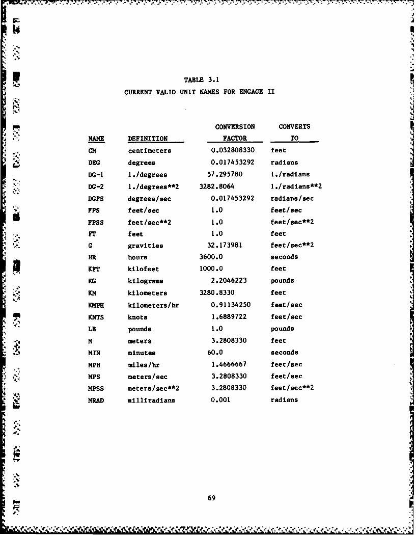
17%(4

CTABLE 3.1

CURRENT VALID UNIT NAMES FOR ENGAGE II

CONVERSION CONVERTS

NAME DEFINITION FACTOR TO

CM centimeters 0.032808330 feet

DEG degrees 0.017453292 radians

DG-1 1./degrees 57.295780 1./radians

DG-2 l./degrees**2 3282.8064 I./radians**2

DGPS degrees/sec 0.017453292 radians/sec

FPS feet/sec 1.0 feet/sec

FPSS feet/sec**2 1.0 feet/sec**2

, ,. FT feet 1.0 feet

G gravities 32.173981 feet/sec**2

HR hours 3600.0 seconds

KFT kilofeet 1000.0 feet

KG kilograms 2.2046223 pounds

* KM kilometers 3280.8330 feet

KMPH kilometers/hr 0.91134250 feet/sec

* KNTS knots 1.6889722 feet/sec

* LB pounds 1.0 pounds

N meters 3.2808330 feet

MIN minutes 60.0 seconds

MPH miles/hr 1.4666667 feet/sec

j * MPS meters/sec 3.2808330 feet/sec

MPSS meters/sec**2 3.2808330 feet/sec**2

MRAD milliradians 0.001 radians

69

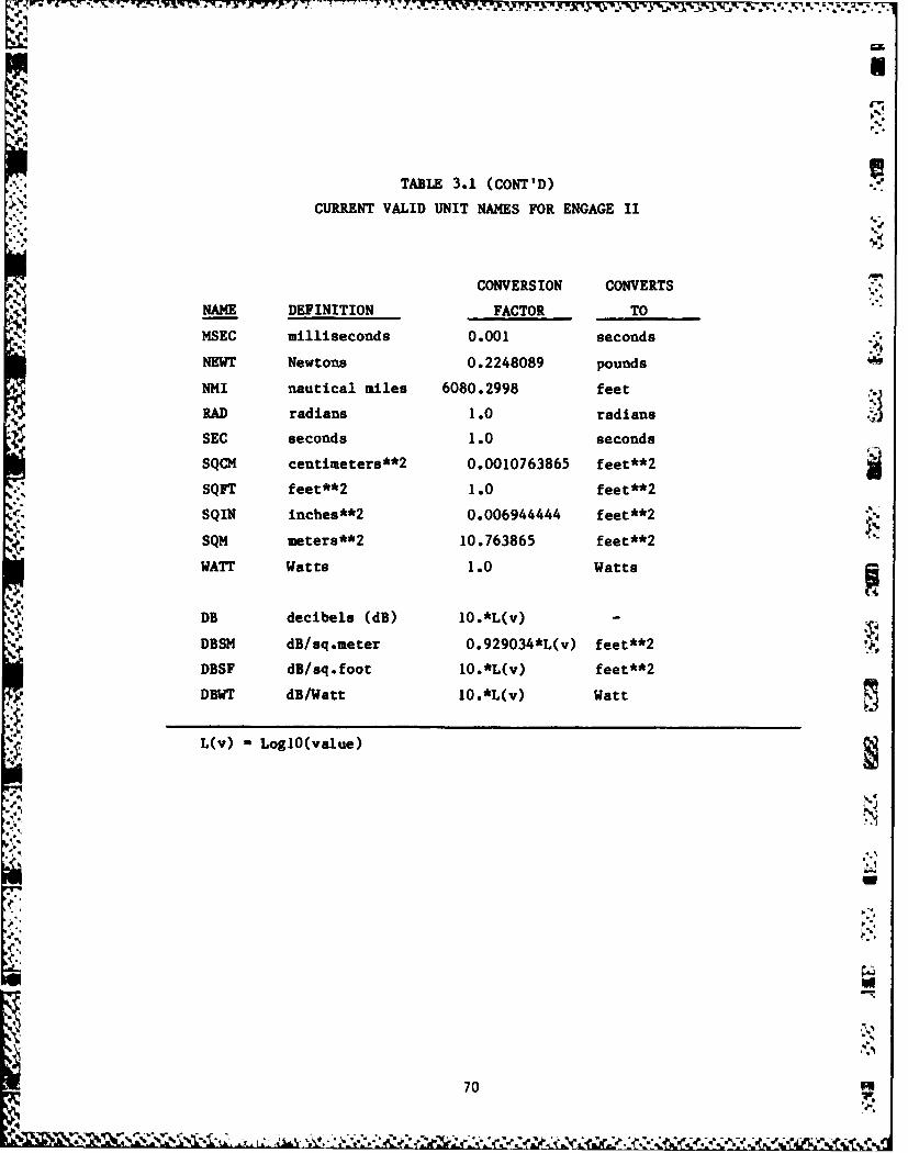
TABLE 3.1 (CONT'D)

CURRENT VALID UNIT NAMES FOR ENGAGE II

CONVERSION CONVERTS

NAME DEFINITION FACTOR TO

MSEC milliseconds 0.001 seconds

NEWT Newtons 0.2248089 pounds

NMI nautical miles 6080.2998 feet

gAD radians 1.0 radians

SEC seconds 1.0 seconds

SQCM centimeters**2 0.0010763865 feet**2

SQFT feet**2 1.0 feet**2

". SQIN inches**2 0.006944444 feet**2

SQM meters**2 10.763865 feet**2

WATT Watts 1.0 Watts

DB decibels (dB) 10.*L(v)-

DBSM dB/sq.meter 0.929034*L(v) feet**2

DBSF dB/sq.foot 10.*L(v) feet**2

DBWT dB/Watt 10.*L(v) Watt

L(v) LoglO(value)

70

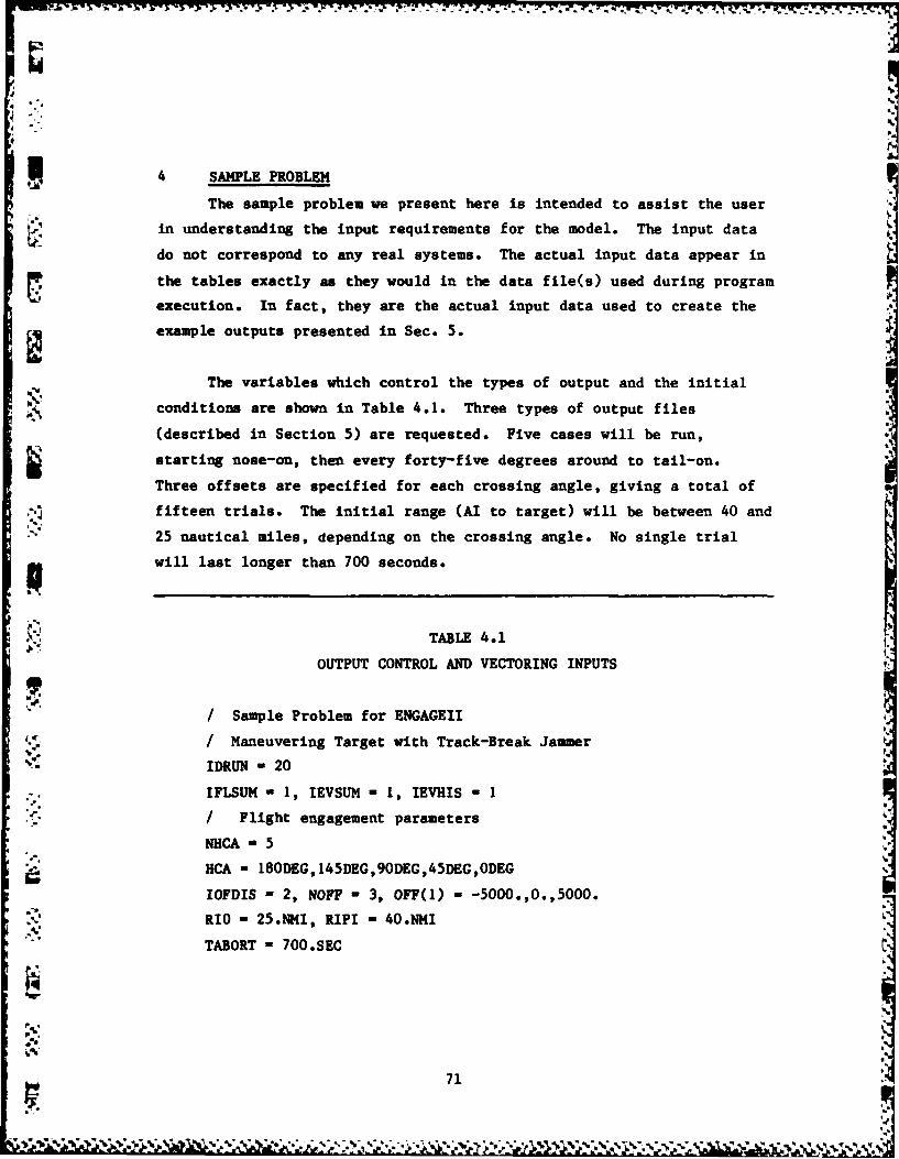
4 SAMPLE PROBLEM

The sample problem we present here is intended to assist the user

in understanding the input requirements for the model. The input data

do not correspond to any real systems. The actual input data appear in

the tables exactly as they would in the data file(s) used during program

execution. In fact, they are the actual input data used to create the

example outputs presented in Sec. 5.

The variables which control the types of output and the initial

conditions are shown in Table 4.1. Three types of output files

(described in Section 5) are requested. Five cases will be run,

starting nose-on, then every forty-five degrees around to tail-on.Three offsets are specified for each crossing angle, giving a total of

:4. fifteen trials. The initial range (A to target) will be between 40 and

25 nautical miles, depending on the crossing angle. No single trial

p will last longer than 700 seconds.

TABLE 4.1

OUTPUT CONTROL AND VECTORING INPUTS

/ Sample Problem for ENGAGEII

/ Maneuvering Target with Track-Break Jammer

IDRUN - 20

IFLSUM - 1, IEVSUM - 1, IEVHIS - 1

/ Flight engagement parameters

NHCA 5

HCA = 180DEG,145DEG,90DEG,45DEG,ODEG

IOFDIS - 2, NOFF - 3, OFF(1) - -5000.,0.,5000.RIO - 25.N1M, RIPI - 40.NMI

TABORT = 700.SEC

71o,,

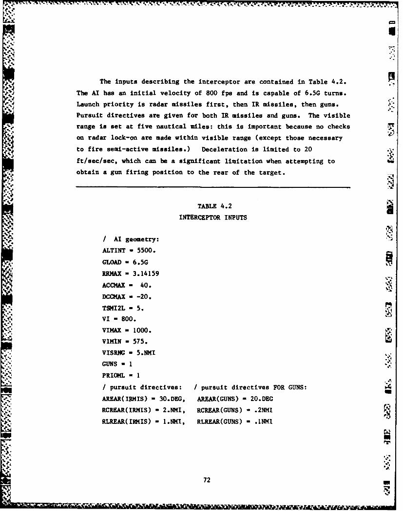
The inputs describing the interceptor are contained in Table 4.2.

The AI has an initial velocity of 800 fps and is capable of 6.5G turns.-,..

Launch priority is radar missiles first, then IR missiles, then guns.

Pursuit directives are given for both IR missiles and guns. The visible

range is set at five nautical miles: this is important because no checks

on radar lock-on are made within visible range (except those necessary

to fire semi-active missiles.) Deceleration is limited to 20

ft/sec/sec, which can be a significant limitation when attempting to

obtain a gun firing position to the rear of the target.

TABLE 4.2

INTERCEPTOR INPUTS

/ AI geometry:

ALTINT - 5500.

.,* GLOAD - 6.5G

* tRRMAX - 3.14159

ACCMAX - 40.

DCCMAX - -20.

TSKI2L - 5.

VI = 800.VIMAX - 1000.

VIMIN - 575.

VISRNG - 5.NMI

GUNS -1

PRIOL 1

/ pursuit directives: / pursuit directives FOR GUNS:

AREAR(IRMIS) - 30.DEG, AREAR(GUNS) - 20.DEG

RCREAR(IRMIS) - 2.NMI, RCREAR(GUNS) - .2NMI

RLREAR(IRMIS) - I.NMI, RLREAR(GUNS) - .LNMI

72

- -

The AI is equipped with two sensors: a radar and a passive

djunct. The performance of these two sensors is described in Table 4.3.

The first two segments of the Table include the timing inputs. The time

steps during acquisition (TSACQ) and track (TSTRK) are not actually

radar parameters, but simulation time steps. The user must choose time

steps based on the fidelity required, realizing that smaller time steps

. will increase the run time. One second has been found to be a good

compromise for subsonic intercepts, As the target or AI velocities are

V increased, TSTRK must be reduced. There is a third time step (TSREAR,

not used in this example) which may be used during the conversion to

rear-hemisphere IR or gun firing positions. High line-of-sight rates

may occur during these phases, and it may be necessary to use time steps

as small as .1 to .2 seconds.

The radar has both high- and medium-PRF modes. The high-PRF mode

performs better in a clutter-free environment (RZERO(AI-HI)), and the

medium-mode is superior in clutter (RI(AI-HED)). The variables

beginning with AVGPWR and ending with ALOSSJ are used for main-lobe

. clutter and jamming calculations (see Appendices A and B). The scope-

limited detection range is 60 nautical miles. The scan pattern is four

elevation bars by +60 degrees in azimuth. Most radars have several

optional settings for RSCOPE, AZSCAN and ELBARS, and a continuous range

for ELCTR. These would be set according to where the controlling agency

advised the pilot to look for the target.'-The AI radar has a track-on-jam option(TOJ-1), but this cannot be

used in this example since the Janming is a track-breaker. Track-on-jam

is considered to be usable only against noise jamming. TJEFF is the

threshold J/S ratio the jamming must exceed in order to break track.

.,'7

• 73,I,

i '- * 5S-

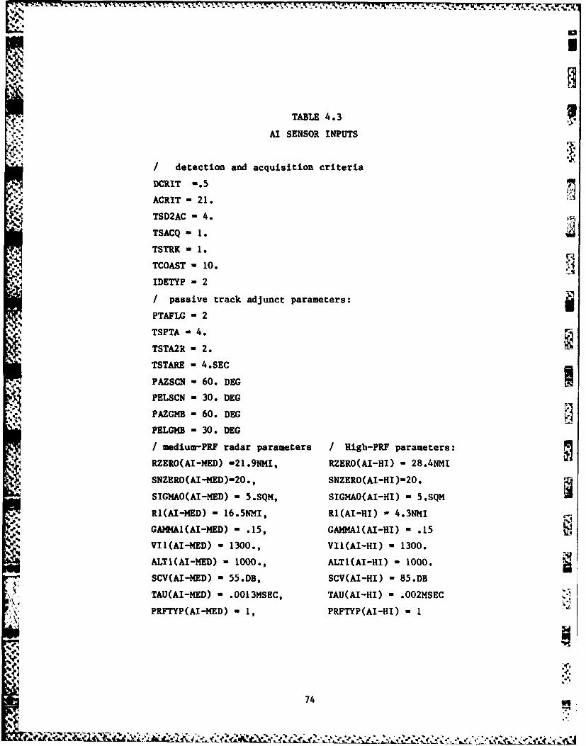
* TABLE 4.3

AI SENSOR INPUTS

/ detection and acquisition criteriaDCRIT -.5

ACRIT - 21.

TSD2AC - 4.'V TSACQ - 1.

TSTRK -1.

TCOAST - 10.

IDETYP - 2

/ passive track adjunct parameters:

PTAFLG - 2

TSPTA -4.

TSTA2R - 2.

TSTARE - 4.SEC

PAZSCN - 60. DEGU

PELSCN - 30.* DEG

PAZGMB - 60. DEG

PELGHB - 30. DEG

/ uediuu-PRF radar parameters /High-PRF parameters:

RZERO(AI-MED) -21.9NMI, RZERO(AI-HI) - 28.4NMI

SNZERO(AI-HD)-20., SNZERO(AI-H)-20.

SIGMA0(AI-IED) - 5.SQM, SIGMAO(AI-HI) - 5.SQM

Rl(AI-MED) - 16.5NMI, R1(AI-HI) - 4.3NHI

GAMMAI(AI-MED) - .15, GAMMA1(AI-HI) - .15

VII(AI-MED) - 1300., VII(AI-HI) - 1300.

ALTI(AI-MED) - 1000., ALT1(AI-HI) - 1000.

SCV(AI-MED) - 55.DB, SCV(AI-HI) - 85.DB

TAU(AI-MED) - .OOI3MSEC, TAU(AI-HI) -. OO2MSEC

PRFTYP(AI-MED) -1, PRFTYP(AI-HI) I

97

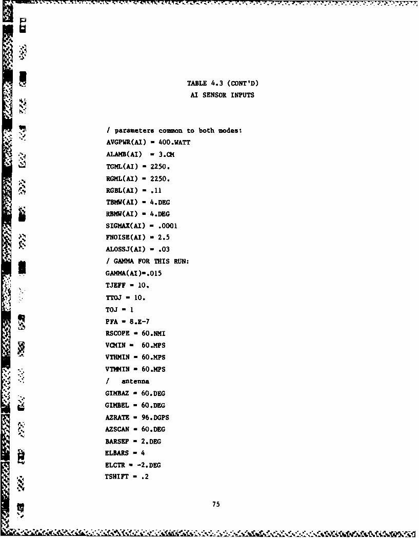
TABLE 4.3 (CONT'D)

AI SENSOR INPUTS

Iparameters common to both modes:

AVGPWR(AI) - 400.WATT

ALAMB(AI) - 3.Q4

TGML(AI) - 2250.

*RGML(AI) - 2250.

RGBL(AI) - .11

TBWAI) - 4.DEG

RBMW(AI) - 4.DEG,

SIGMAX(AI) - .0001

FNOISE(AI) - 2.5

ALOSSJ(AI) - .03

/ GAMMA FOR THIS RUN:I GAIMA(AI )-.015

TJEFF - 10.

TTOJ -10.

TOJ 1

PFA -8.E-7

RSCOPE - 60.NMI

VCHIN - 60 .MPS

VTHMIN - 60.MPS

* VTM*IIN - 60.MPS

* I antennaGIBZ-6.E

GIMBEL - 60.DEG

AZRATE - 96.DGPS

AZSCAN - 60.DEGI:BARSEP - 2.DEG

ELCTR -- 2.DEG

4 TSHIFT - .2

75

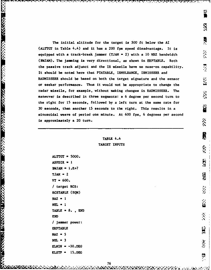
* * * &t. -. 7'.1771b3-7-77 * St.. .7

The initial altitude for the target is 500 ft below the AI

• (ALTTGT in Table 4.4) and it has a 200 fps speed disadvantage. It is

equipped with a track-break jammer (TJAM - 2) with a 10 MHZ bandwidth

(BWJA)o. The jamming is very directional, as shown in ERPTABLE. Both

the passive track adjunct and the IR missile have no nose-on capability.

It should be noted here that PTATABLE, IRMSLRANGE, IRMISSERR and

RADMISSERR should be based on both the target signature and the sensor

or seeker performance. Thus it would not be appropriate to change the

radar missile, for example, without making changes in RADMISSERR. The

maneuver is described in three segments: a 6 degree per second turn to

the right for 15 seconds, followed by a left turn at the same rate for

30 seconds, then another 15 seconds to the right. This results in a

sinusoidal weave of period one minute. At 600 fps, 6 degrees per second

is approximately a 2G turn. CS

TABLE 4.4

TARGET INPUTS

ALTTGT - 5000.

ASPDIR - 1

BWJAM - I.E+7

TJAM - 2

VT - 600.

/ target RCS:

RCSTABLE (SQM)

NAZ -I

NEL= I

TABLE - 8. , END

* END/ jammer power:

ERPTABLE

NAZ - 5

* NEL - 3

ELMIN - -30.DEG

ELSTP - 15.DEG

76i

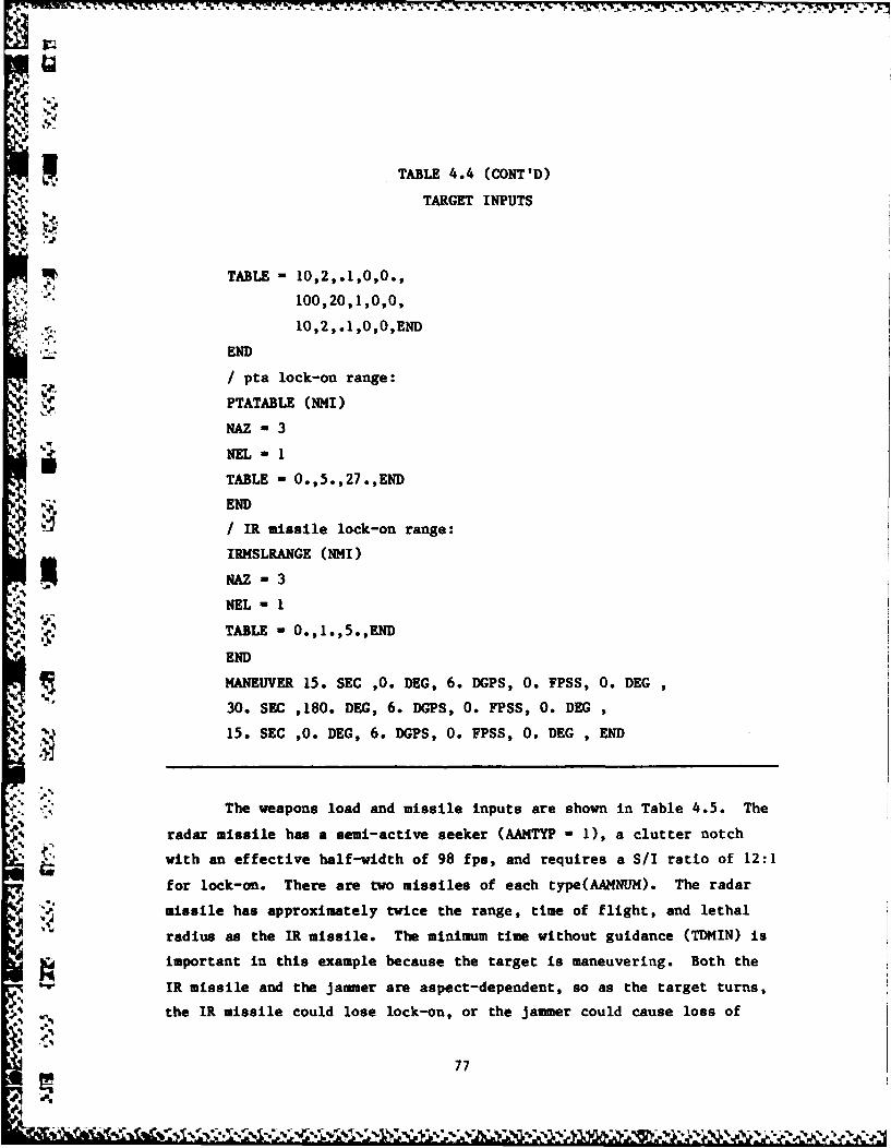
, o

TABLE 4.4 (CONT'D)

TARGET INPUTS

TABLE 1 0,2,.1,0,0.,

100,20,1,0,0,

10,2,.1,0,0,END

END

/ pta lock-on range:

PTATABLE (NMI)

NAZ-3

NEL-I

TABLE - 0.,5.,27.,END

END

/ IR missile lock-on range:

IRMSLRANGE (NMI)

IlAZ - 3

NEL -1

. . ~. TABLE - O.,1.,5.,END

END

MANEUVER 15. SEC ,0. DEG, 6. DGPS, 0. FPSS, 0. DEG

30. SEC ,180. DEG, 6. DGPS, 0. FPSS, 0. DEG ,

'I 15. SEC ,0. DEG, 6. DGPS, 0. FPSS, 0. DEG , END

The weapons load and missile inputs are shown in Table 4.5. The

radar missile has a semi-active seeker (AAMTYP - 1), a clutter notch

with an effective half-width of 98 fps, and requires a S/I ratio of 12:1

for lock-on. There are two missiles of each type(AAMNUM). The radar

missile has approximately twice the range, time of flight, and lethal

radius as the IR missile. The minimum time without guidance (TDMIN) is

important in this example because the target is maneuvering. Both the

IR missile and the jammer are aspect-dependent, so as the target turns,

the IR missile could lose lock-on, or the jammer could cause loss of

77

U. Up i~- . *,' ~ * ~ *** - V ' -- -.. ~ '

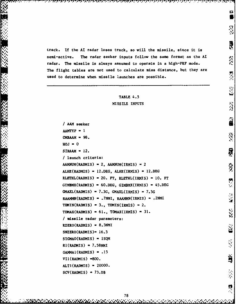
_ 0X

track. If the AI radar loses track, so will the missile, since it is

semi-active. The radar seeker inputs follow the same format as the AI

radar. The missile is always assumed to operate in a high-PRF mode.

The flight tables are not used to calculate miss distance, but they are

used to determine when missile launches are possible.

TABLE 4.5

MISSILE INPUTS

/ AAM seeker

AAMTYP - 1

*CMBAAM - 98.

HOJ 0

SIRAAM - 12.

/ launch criteria:

AAMNUM(RADMIS) - 2, AAMNUM(IRMIS) = 2

ALHE(RADMIS) - 12.DEG, ALHE(IRMIS) = 12.DEG

RLETHL(RADMIS) - 20. FT, RLETHL(IRMIS) - 10. FT

GIMBMX(RADMIS) - 60.DEG, GIMBMX(IRMIS) - 45.DEG

GMAXL(RADMIS) - 7.3G, GMAXL(IRMIS) - 7.3G

RATAN(RADMIS) - .7NMI, RAAMMN(IRMIS) - .2NMITDMIN(RADMIS) - 3., TDMIN(IRMIS) -2.

TDMAX(RADMTS) - 61., TDMAX(IRMIS) 31.

missile radar parameters:

RZERO(RADMIS) - 8.3NMI

SNZERO(RADMIS)- 16.3

SIGMA0(RADMIS) - ISQM

RI(RADMIS) - 7.58NMI

GAIIMAt(RADMIS) - .15VII(RAD4IS) =800.

ALTI(RADMIS) - 20000.

SCV(RADMIS) - 73.DB

78rzt* e: r. .'.

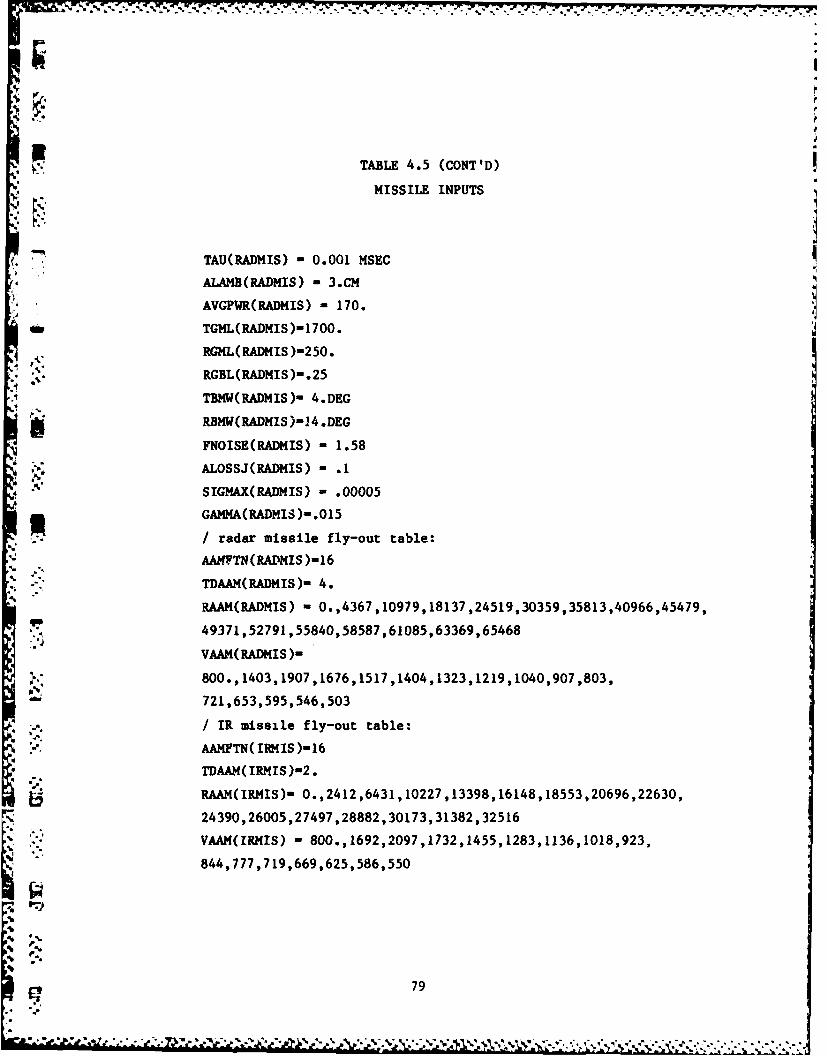
TABLE 4.5 (CONT'D)

MISSILE INPUTS

TAU(RADMIS) - 0.001 MSEC

ALAMB(RADMIS) - 3.CM

AVGPWR(RADMIS) - 170.

TGML(RADMIS)- 1700.

RGML(RADMIS))-250.

• RGBL(RADMIS)-.25

TBMW(RADMIS )- 4.DEG

RBMW(RADMIS )-] 4 .DEG

FNOISE(RADMIS) - 1.58

ALOSSJ(RADMIS) - .1

SIGMAX(RADMIS) - .00005

GAMMA(RADMIS )-.015

/ radar missile fly-out table:

y -AAMFTN(RADMIS)-16

TDAAM(RADMIS)- 4.

RAAM(RADMIS) - 0.,4367,10979,18137,24519,30359,35813,40966,45479,

49371,52791,55840,58587,61085,63369,65468

VMM(RADMIS )-

800.,1403,1907,1676,1517,1404,1323,1219,1040,907,803,

721,653,595,546,503

/ IR missile fly-out table:AAMFTN(IRMIS)-16

TDAAM(IRMIS)-2.

RAAM(IRMIS)- 0.,2412,6431,10227,13398,16148,18553,20696,22630,

24390,26005,27497,28882,30173,31382,32516

VAAM(IRIS) - 800.,1692,2097,1732,1455,1283,1136,1018,923,

844,777,719,669,625,586,550

9,

4.

. . . ..,

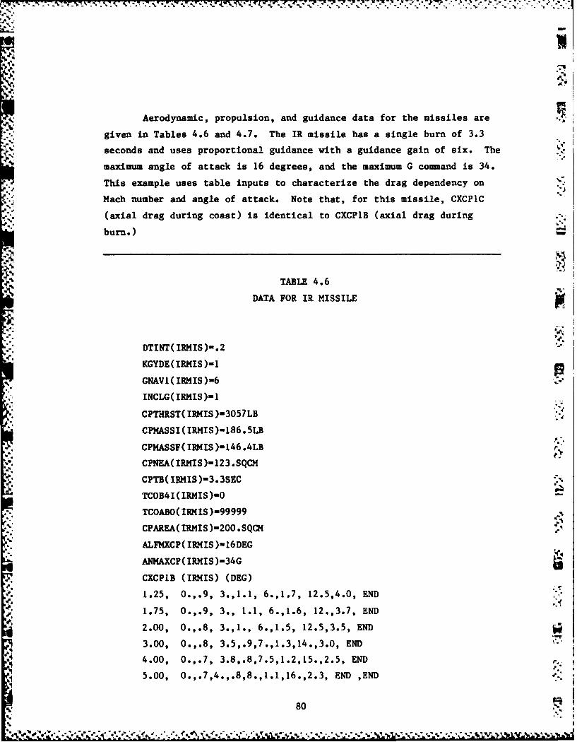
i

Aerodynamic, propulsion, and guidance data for the missiles are

given in Tables 4.6 and 4.7. The IR missile has a single burn of 3.3

seconds and uses proportional guidance with a guidance gain of six. The

maximum angle of attack is 16 degrees, and the maximum G command is 34.

This example uses table inputs to characterize the drag dependency on

Mach number and angle of attack. Note that, for this missile, CXCPIC

(axial drag during coast) is identical to CXCPIB (axial drag during

burn.)

TABLE 4.6

DATA FOR IR MISSILE

DTINT( IRMIS )- .2

KGYDE(IRMIS)-1

GNAVI(IRMIS)-6

INCLG( IRMIS )-1

CPTHRST( IRMIS )-3057LB "-

CPMASSI ( IRMIS )-186 . 5LB

CPMASSF( IRMIS )-146.4LB

CPNEA(IRMIS) 123.SQCM

CPTB(IRMIS)-3.3SEC

TCOB4I(IRMIS)-0

TCOABO( IRMIS)-99999

CPAREA( IRMIS )-200 .SQCM

ALFMXCP( IRMIS )-16DEG

ANMAXCP( IRMIS )-34G

CXCPIB (IRMIS) (DEG)

1.25, 0.,.9, 3.,1.1, 6.,1.7, 12.5,4.0, END

'. 1.75, O.,.9, 3., 1.1, 6.,1.6, 12.,3.7, END

2.00, 0.,.8, 3.,1., 6.,1.5, 12.5,3.5, END

3.00, 0.,.8, 3.5,.9,7.,1.3,14.,3.0, END

4.00, O.,.7, 3.8,.8,7.5,1.2,15.,2.5, END r.

5.00, O.,.7,4.,.8,8.,1.1,16.,2.3, END ,END

80-* .. %

.

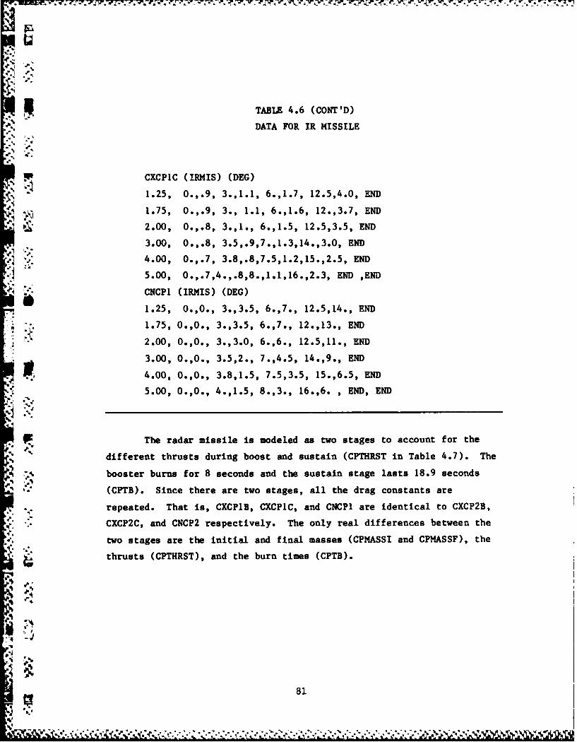
TABLE 4.6 (CONT'D)

DATA FOR IR MISSILE

CXCP1C (IRMIS) (DEG)1.25, 0.,.9, 3.,1.1, 6.,1.7, 12.5,4.0, END

1.75, 0.,.9, 3., 1.1, 6.,1.6, 12.,3.7, END

2.00, 0.,.8, 3.,I., 6.,1.5, 12.5,3.5, END3.00, 0.,.8, 3.5,.9,7.,1.3,14.,3.0, END

4.00, 0.,.7, 3.8,.8,7.5,1.2,15.,2.5, END

5.00, O.,.7,4.,.8,8.,1.1,16.,2.3, END ,END

CNCP1 (IRMIS) (DEG)

1.25, 0.,0., 3.,3.5, 6.,7., 12.5,14., END

. 1.75, 0.,0., 3.,3.5, 6.,7., 12.,13., END

2.00, 0.,0., 3.,3.0, 6.,6., 12.5,11., END

3.00, 0.,0., 3.5,2., 7.,4.5, 14.,9., END

4.00, 0.,0., 3.8,1.5, 7.5,3.5, 15.,6.5, END

5.00, 0.,0., 4.,1.5, 8.,3., 16.,6. , END, END

PC The radar missile is modeled as two stages to account for the

Rb % different thrusts during boost and sustain (CPTHRST in Table 4.7). The

booster burns for 8 seconds and the sustain stage lasts 18.9 seconds

(CPTB). Since there are two stages, all the drag constants are

repeated. That is, CXCP1B, CXCPIC, and CNCP1 are identical to CXCP2B,

CXCP2C, and CNCP2 respectively. The only real differences between the

two stages are the initial and final masses (CPMASSI and CPMASSF), the

thrusts (CPTHRST), and the burn times (CPTB).

81

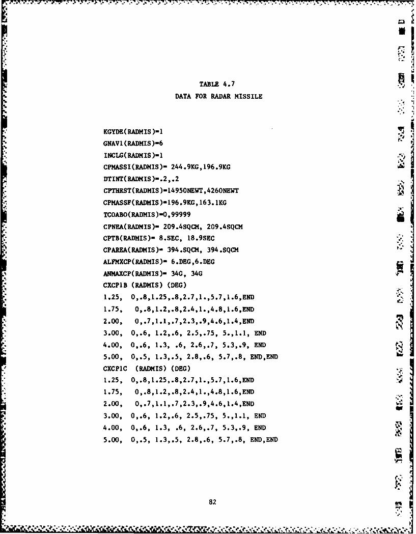
TABLE 4.7

DATA FOR RADAR MISSILE

KGYDE(RADMIS )-1

GNAV1 (RADMIS )-6

INCLG(RADmis )-1CPMASSI(RADMIS)" 244.9KG,196.9KG

DTINT(RADMIS)"'.2,.2 -

CPTHRST(RADNIS )-L495ONEWT,426ONEWT

CPMASSF(RADMIS)-196.9KG,163.IKG

TCOABO(RADMIS )-O ,99999

CPNEA(RADMIS)- 209.4SQCl4, 209.4SQCM

CPTB(RADMIS)- 8.SEC, 18.9SEC

CPAREA(RADMIS)- 394.SQCl4, 394.SQCM I

ALFMXCP(RADMIS)- 6.DEG,6.DEG

ANMAXCP(RADMIS)- 34G, 34G

CXCPlB (RADMIS) (DEG)

41.25, O,.8,1.25,.8,2.7,1.,5.7,1.6,END

1.75, O,.8,1.2,.8,2.4,1.,4.8,1.6,END

2.00, O,.7,1.1,.7,2.3,.9,4.6,1.4,END

3.00, 0,.6, 1.2,.6, 2.5,.75, 5.,1.1, END

4.00, 0,.6, 1.3, .6, 2.6,.7, 5.3,.9, END

5.00, 0,.5, 1.3,.5, 2.8,.6, 5.7,.8, END,END

CXCPIC (RADMIS) (DEG) -

1.25, O,.8,1.25,.8,2.7,1.,5.7,1.6,END

1.75, 0,.8,1.2,.8,2.4,1 .,4.8,1.6,END

2.00, 0,.7, 1.1, .7,2.3,.9,4.6, I.4,END

3.00, 0,.6, 1.2,.6, 2.5,.75, 5.,1.1, END

4.00, 0,.6, 1.3, .6, 2.6,.7, 5.3,.9, END

5.00, 0,.5, 1.3,.5, 2.8,.6, 5.7,.8, END,END

82

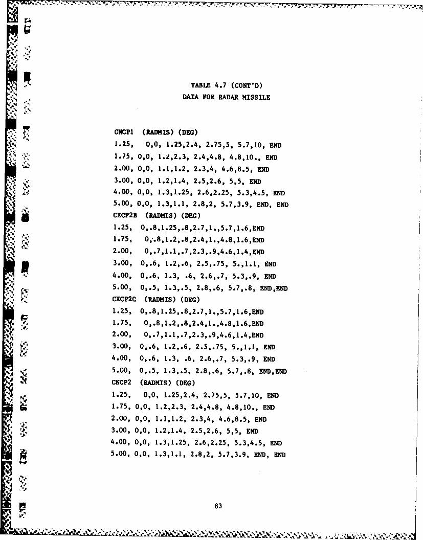
p.,

-A

TABLE 4.7 (CONT'D)DATA FOR RADAR MISSILE

p.

CNCPI (RADMIS) (DEG)

1.25, 0,0, 1.25,2.4, 2.75,5, 5.7,10, END

' " 1.75, 0,0, 1a,2.3, 2.4,4.8, 4.8,10., END

2.00, 0,0, 1.1,1.2, 2.3,4, 4.6,8.5, END

3.00, 0,0, 1.2,1.4, 2.5,2.6, 5,5, END

4.00, 0,0, 1.3,1.25, 2.6,2.25, 5.3,4.5, END

5.00, 0,0, 1.3,1.1, 2.8,2, 5.7,3.9, END, END

CXCP2B (RADMIS) (DEG)

1.25, O,.8,1.25,.8,2.7,1.,5.7,1.6,END

C.'. 1.75, 0,.8 ,1.2,.8,2.4,1.,4.8,1.6,END

" 2.00, O,.7,1.1,.7,2.3,.9,4.6,1.4,END

3.00, 0,.6, 1.2,.6, 2.5,.75, 5.,1.1, END

--- 4.00, 0,.6, 1.3, .6, 2.6,.7, 5.3,.9, END

5.00, 0,.5, 1.3,.5, 2.8,.6, 5.7,.8, END,END

CXCP2C (RADMIS) (DEG)

1.25, 0,.8,1.25,.8,2.7,1.,5.7,1.6,ENDI !..1.75, O,.8,1.2,.8,2.4,1°,4.8,1.6,END

2.00, 0,.7,1.1,.7,2.3,.9,4.6,1.4,ENB

3.00, 0,*6, 1.2,*6, 2*5,*75, 5*,1.1, ENDLe 4.00, 0,.6, 1.3, .6, 2.6,.7, 5.3,.9, END

5.00, 0,.5, 1.3,.5, 2.8,.6, 5.7,.8, END,END

1' CNCP2 (RADMIS) (DEG)

1.25, 0,0, 1.25,2.4, 2.75,5, 5.7,10, END

1.75, 0,0, 1.2,2.3, 2.4,4.8, 4.8,10., END

2.00, 0,0, 1.1,1.2, 2.3,4, 4.6,8.5, END

3.00, 0,0, 1.2,1.4, 2.5,2.6, 5,5, END

4.00, 0,0, 1.3,1.25, 2.6,2.25, 5.3,4.5, END

5.00, 0,0, 1.3,1.1, 2.8,2, 5.7,3.9, END, END

p 83

1A t

AA

5 ENGAGE II OUTPUT

ENGAGE II can generate several different output files, depending

on the options selected by the user. All files have an identical

heading, giving the date, time, and run number of the run; and an input

sunmary page. A sample of the output heading and the input summary are

included as Fig. 5.1 and Fig. 5.2. These samples, and all those

included to illustrete the following output files, have been generated

vith the input file described in Section 4. "

A brief description of each of these output files follows.

'V5.1 EVENT HISTORY FILE

* This file describes the events occurring in each engagement in the

run. There is one engagement per page, identified by the Heading

Crossing Angle and the initial Offset of the engagement. Then each

event Is listed, with the following information:

* The Event name.

* The time of the event.

0 The AI X and Y coordinates at the time of the event.

4~0 The target X and Y coordinates at the time of the event.

. The location of the Al relative to the target, in

4 X, Y, and Z coordinates, at the time of the event.

* Further comments about the event.

The comments referred to in Item 6 vary with the event type. Table 5.1

lists the various comments and briefly describes them.

* This file is generated when the value of user-input IEVHIS is 1.

Figure 5.3 illustrates an example of this output.

84

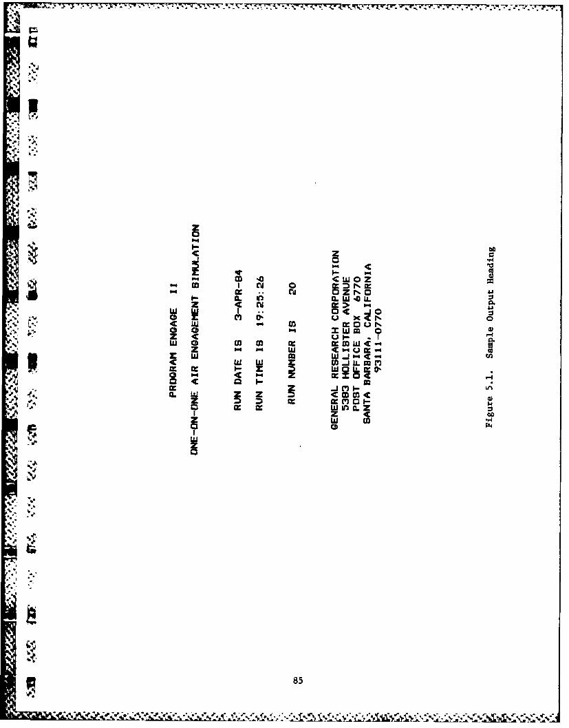
4c

~0

0" c~ o

.4O

I umI'rd0z

O- u -

z P4 0- ru mx Lu I _j " C

cc 0:xW0L=V-0 4c xw 0

z <

w 0

.4P-

44

485

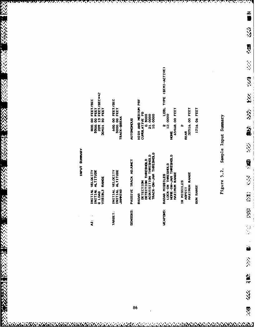
rd..

u U. Cw 4cc>m mILI.

wwww wUj LL LU 1

g 0

04 g ri.

In w Nv

l'4 - *

WWWw CAI0 w

ic ~ W Ill1 -4Ju

Aw w

02

021- W -

z-z -z

02i

* al

0 02 86

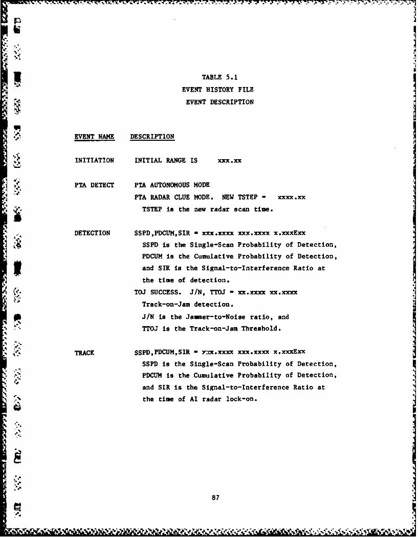
TABLE 5.1

EVENT HISTORY FILE

EVENT DESCRIPTION

EVENT NAME DESCRIPTION

INITIATION INITIAL RANGE IS XXx.xx

I :) PTA DETECT PTA AUTONOMOUS MODEPTA RADAR CLUE MODE. NEW TSTEP - xxxx.xx

TSTEP is the new radar scan time.

DETECTION SSPD,PDCUM,SIR - xxx.xxxx xxx.xxxx x.xxxExx

SSPD is the Single-Scan Probability of Detection,

PDCUM is the Cumulative Probability of Detection,

and SIR is the Signal-to-Interference Ratio at

the time of detection.

TOJ SUCCESS. J/N, TTOJ - xx.xxxx xx.xxxx

Track-on-Jam detection.

J/N is the Jamer-to-Noise ratio, andTTOJ is the Track-on-Jam Threshold.

TRACK SSPD,PDCUM,SIR - 7. xxxx xxx.xxxx x.xxxExx

SSPD is the Single-Scan Probability of Detection,

*PDCUM is the Cumulative Probability of Detection,

and SIR is the Signal-to-Interference Ratio at

the time of AI radar lock-on.

87

O .

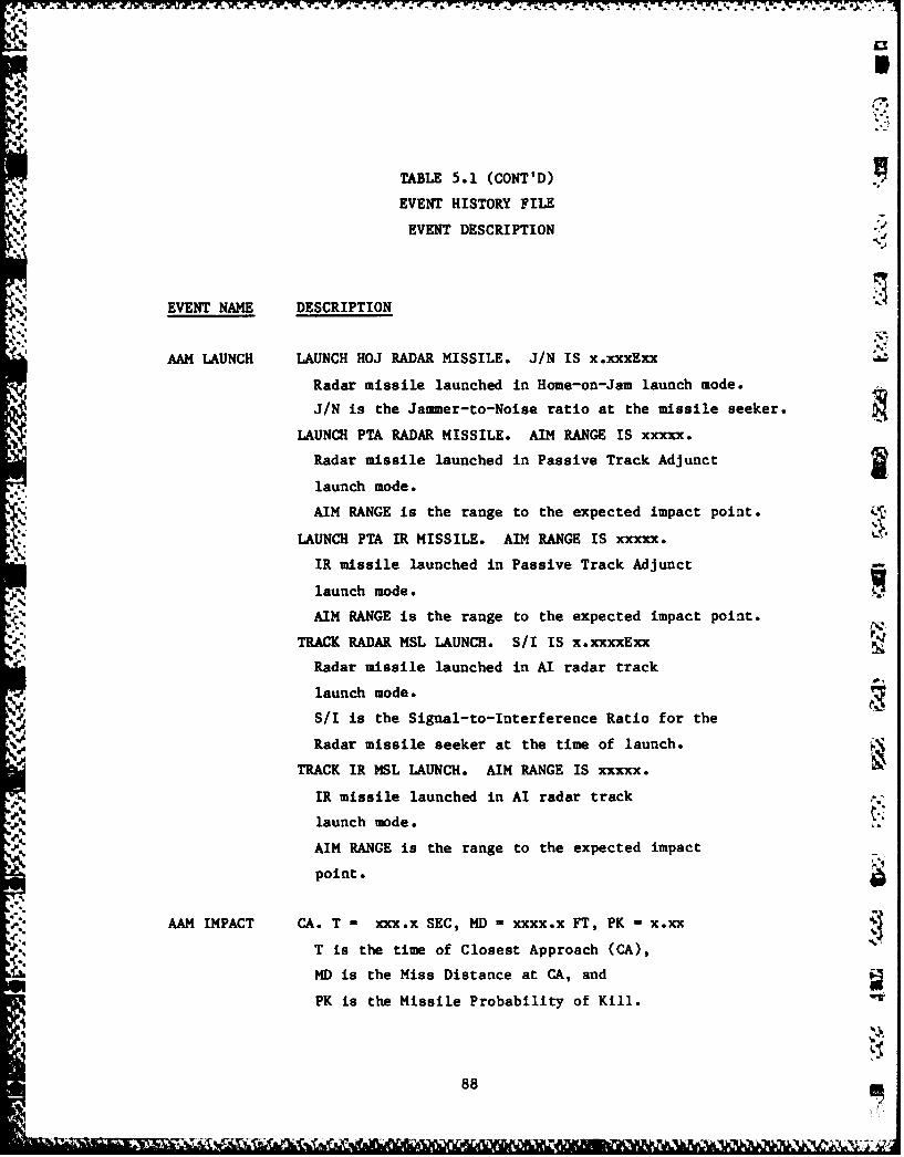
TABLE 5.1 (CONT'D)

EVENT HISTORY FILE

EVENT DESCRIPTION

EVENT NAME DESCRIPTION

AAM LAUNCH LAUNCH HOJ RADAR MISSILE. J/N IS x.xxxExx

Radar missile launched in Home-on-Jam launch mode.

JIN is the Jammer-to-Noise ratio at the missile seeker.

LAUNCH PTA RADAR MISSILE. AIM RANGE IS xxxxx.

Radar missile launched in Passive Track Adjunct

launch mode.

AIM RANGE is the range to the expected impact point.

LAUNCH PTA IR MISSILE. AIM RANGE IS xxxxx.

IR missile launched in Passive Track Adjunct

launch mode.

AIM RANGE is the range to the expected impact point.

TRACK RADAR MSL LAUNCH. S/I IS x.xxxxExx

Radar missile launched in AI radar track

launch mode.

S/I is the Signal-to-Interference Ratio for the

Radar missile seeker at the time of launch.TRACK IR MSL LAUNCH. AIM RANGE IS xxxxx.

IR missile launched in AI radar track

launch mode. a-

AIM RANGE is the range to the expected impact

point.

AAM IMPACT CA. T - xxx.x SEC, MD - xxxx.x FT, PK - x.xx

T is the time of Closest Approach (CA),

MD is the Miss Distance at CA, and

PK is the Missile Probability of Kill. -

88

X l ...... ...

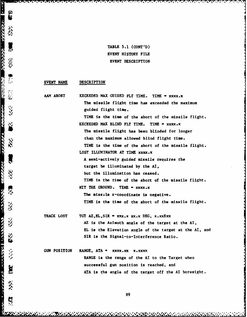
TABLE 5.1 (CONT'D)

EVENT HISTORY FILE

iEVENT DESCRIPTION

EEVENT NAME DESCRIPTION

EVNTNAE DECRPTO

' AAM ABORT EXCEEDED MAX GUIDED FLT TIME. TIME - xxxx.x

The missile flight time has exceeded the maximum

guided flight time.

TIME is the time of the abort of the missile flight.

EXCEEDED MAX BLIND FLT TIME. TIME - xxxx.x

The missile flight has been blinded for longer

than the maximum allowed blind flight time.

4C TIME is the time of the abort of the missile flight.

LOST ILLUMINATOR AT TIME xxxx.x

A semi-actively guided missile requires the

target be illuminated by the AI,but the illumination has ceased.

TIME is the time of the abort of the missile flight.

HIT THE GROUND. TIME - xxxx.x

The missile z-coordinate is negative.

TIME is the time of the abort of the missile flight.

TRACK LOST TGT AZ,EL,SIR - xxx.x xx.x DEG, x.xxExx

AZ is the Azimuth angle of the target at the AI,

* "EL is the Elevation angle of the target at the AI, and

SIR is the Signal-to-Interference Ratio.

GUN POSITION RANGE, ATA - xxxx.xx x.xxxx

RANGE is the range of the AI to the Target when

successful gun position is reached, and

ATA is the angle of the target off the AI boresight.

89

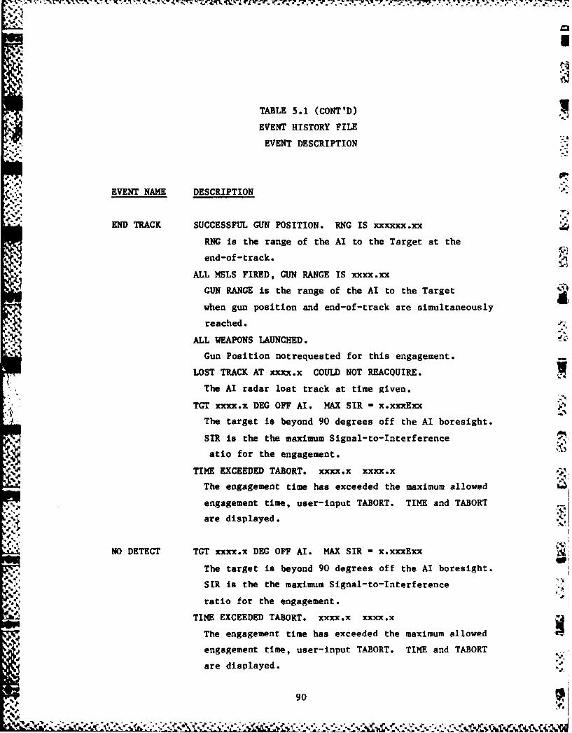
TABLE 5.1 (CONT'D)

EVENT HISTORY FILE

EVENT DESCRIPTION

EVENT NAME DESCRIPTION

END TRACK SUCCESSFUL GUN POSITION. RNG IS xxxxxx.xx

RNG is the range of the AI to the Target at the

end-of-track.

ALL MSLS FIRED, GUN RANGE IS xxxx.xx

GUN RANGE is the range of the AI to the Target

when gun position and end-of-track are simultaneously

reached.

ALL WEAPONS LAUNCHED.

Gun Position notrequested for this engagement.

LOST TRACK AT xxxx.x COULD NOT REACQUIRE.

The AI radar lost track at time given.

, TGT xxxx.x DEG OFF Al. MAX SIR - x.xxxExx

The target is beyond 90 degrees off the AI boresight.

SIR is the the maximum Signal-to-Interference

atio for the engagement.

TIME EXCEEDED TABORT. xxxx.x xxxx.x

The engagement time has exceeded the maximum allowed

engagement time, user-input TABORT. TIME and TABORT

are displayed.

NO DETECT TGT xxxx.x DEG OFF Al. MAX SIR x.xxxExx

-. " The target is beyond 90 degrees off the Al boresight.".,

SIR is the the maximum Signal-to-Interference

ratio for the engagement.

TIME EXCEEDED TABORT. xxxx.x xxxx.x

The engagement time has exceeded the maximum allowed

engagement time, user-input TABORT. TIME and TABORT

are displayed.

90. '

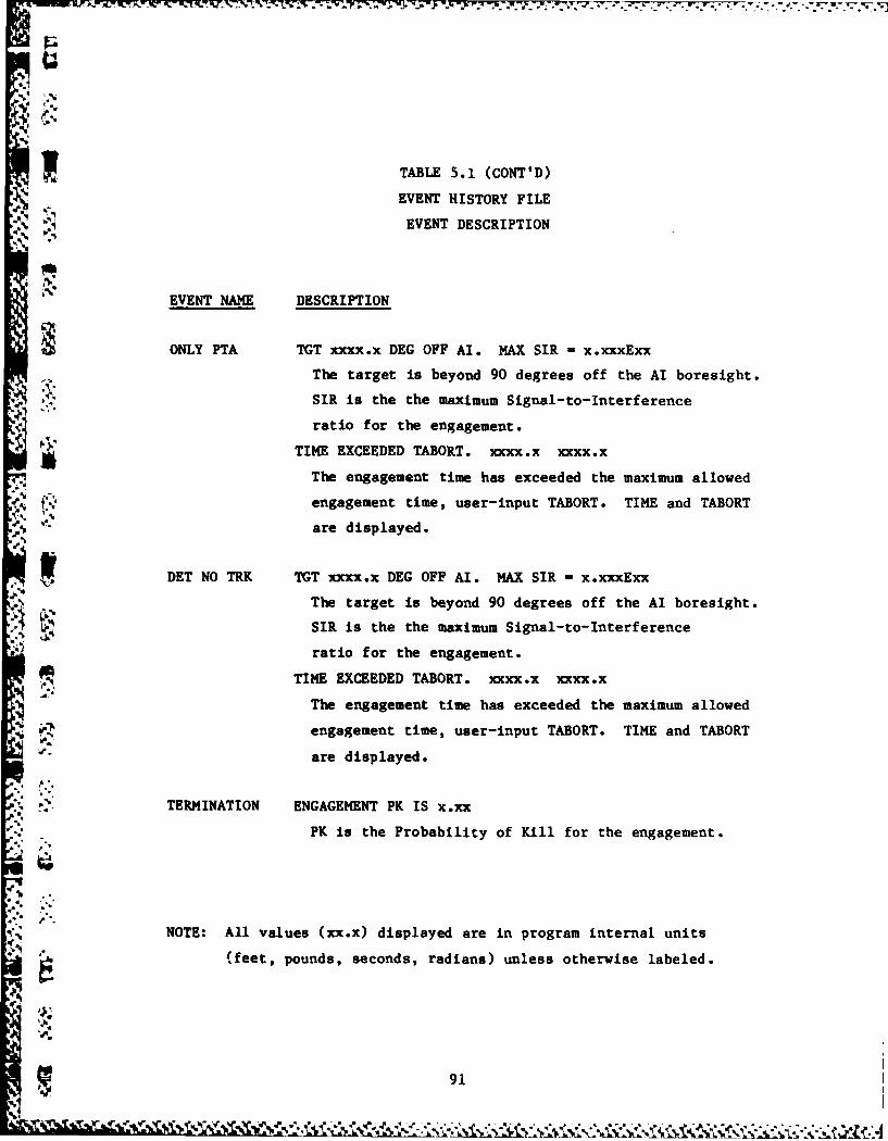
TABLE 5.1 (CONT'D)

EVENT HISTORY FILE

,EVENT DESCRIPTION

EVENT NAME DESCRIPTION

ONLY PTA TGT xxxx.x DEG OFF AI. MAX SIR x.xxxExx

The target is beyond 90 degrees off the AI boresight.

.* SIR is the the maximum Signal-to-Interference

ratio for the engagement.

TIME EXCEEDED TABORT. xxxx.x xxxx.x

The engagement time has exceeded the maximum allowed

f*.' engagement time, user-input TABORT. TIME and TABORT

are displayed.

DET NO TRK TGT xxxx.x DEG OFF AI. MAX SIR - x.xxxExx

The target is beyond 90 degrees off the AI boresight.4 SIR is the the maximum Signal-to-Interference

ratio for the engagement.

TIME EXCEEDED TABORT. xxxx.x xxxx.x

The engagement time has exceeded the maximum allowed

engagement time, user-input TABORT. TIME and TABORT

are displayed.

"; ' TERMINATION ENGAGEMENT PK IS x.xx

PK is the Probability of Kill for the engagement.

NOTE: All values (xx.x) displayed are in program internal units

(feet, pounds, seconds, radians) unless otherwise labeled.

91

I7 M

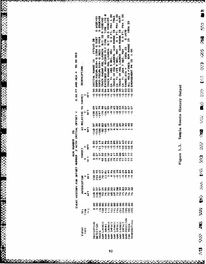
8 ri '0 Snr- 0

% w a 9) t .V .c x 42. V 0

.0 U) CD

) U)2 W W-

-,00 0-MzD ZE .E (

olI 0. , Z-64640-.in 02 z02cc c

0 ~ ~ ~ -Cm ZE.XE Jra~ -D

2M x U - - j CC

m 0 N-O L -C

IL '-0U2I-U40 -)4w

U- 101 w u U l

c I - I-qd0r. u 0C2u0m <2O1-

LL W ..

0

0 &. N. CP I00NmvNN0- v wN&-N' 4

w >

19 N 006o )oo oon

xf

w 0N M-w .0 ,r01n

z ri

.4 04

W ~ ~ ~ -g-. ,M R

U. ~ .OV0-VV - N M> . -4r

CL

LL w~

Q 44Z> at w 0'a 0 - Ma, MN N

z9x 63 0

xi..-

-I.

AD-AU44 119 ENGAGE 11 - SER'S MNANLL(U) GENERAL RESEARCH CORP 212

SANTA BARBARA CA J BALTES ET AL. 31 MAY 84GRC-CR-2 1891 F33615-8i-C-0108

UNCLASSIFIED F/G 5/9 NL

EEEET EE~E

mhI~u1

- .,,

:9U

• **'

Lu,

IV,

. . MICROCOPY RESOLUTION TEST CHART• ,, NATIONAL BUREAU OF STANOAMM -1963-A

;%°..

VP

'mU

-. W .V L4 J4 ~ d ~* V * ~~ k .* ~ . ~ . -. *

5.2 EVENT SUMMARY FILE

This output file (Fig. 5.4) summarizes all occurrences of several

event types for those engagements flown at a single Heading Crossing

Angle (HCA). The top line of the output identifies the HCA. The

selected AI event types are: detection (all types), track, and the

end-of-engagement events. For each event type, the engagement is

identified by index, and the time and relative location of the AI to the

target. A similar summary is generated for the two missile events AAM

~launch and AAM impact. These event summaries are repeated for each HCA

; in the run. The user selects this output by setting the input IEVSUM

to 1.

5.3 FLIGHT SUMMARY FILE

This file contains two short summaries over all engagements in the

run. The file is generated when the input variable IFLSUM is 1. These

summaries are illustrated in Figs. 5.5 and 5.6.

5.3.1 Summary By Engagement

Each engagement is listed on a single line, with the following

information:

e . HCA - Heading Crossing Angle

* OFFSET - Initial Offset distance

0 * RESULTS - a description of the AI detection

*" FAILURE - No detection by AI

PTA DET -- Detection by PTA only

4 RADAR DET -- Detection but not lock-on by AI radar

RADAR TRK - AI radar lock-on achieved.

For Radar Missiles:

" HOJ - Number of radar Missiles Launched in

Home-On-Jam launch mode.

* PTA - Number of radar missiles launched in

~%PTA launch mode.

*~ I.93

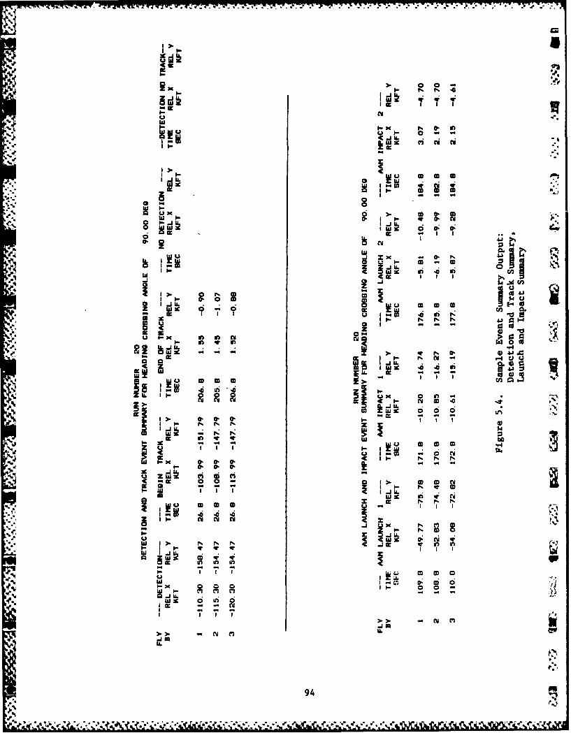
I~.U.

f- A LjU .

w C

WWU UI.- 0 .D.

~*0J WU 00

0 ca

a. 0 0u

I-.JU . . .JIJ. c,w aco a

u 0 -n In rd

In In rd IoVV V4- u7' l4Ew 'w '2 Ni 4) V. I

0 I D Im W In.0 i~

IL I I-.-

U 0-x x0I >

op.0 00 0

I I I 0 00b p otw kx a ai .~I ~ 7 ' 7

c w 0~ 0 CD r

I~ > v

CD

w 39 00

-10 - t

94

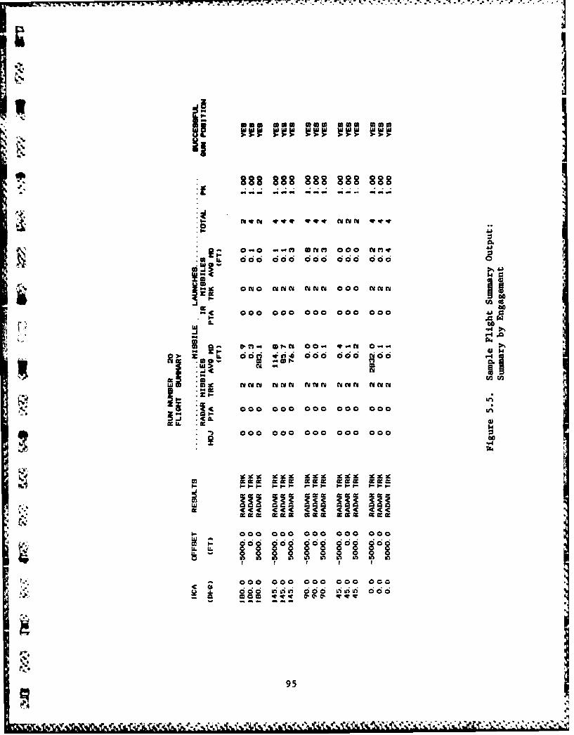
-vwzI T. We Wl. 3 -- -I* 2.J* ? *7-711;

I

** aiE Sn 5 0! nno- n~ -- flflo

00

C 000 000 co coo 000

°°°ooo ooo ooo ooo

C &L 001 0' r-* C' C

95

V.*~ d **J * .* ~* *-' .--. ,.*. - * l

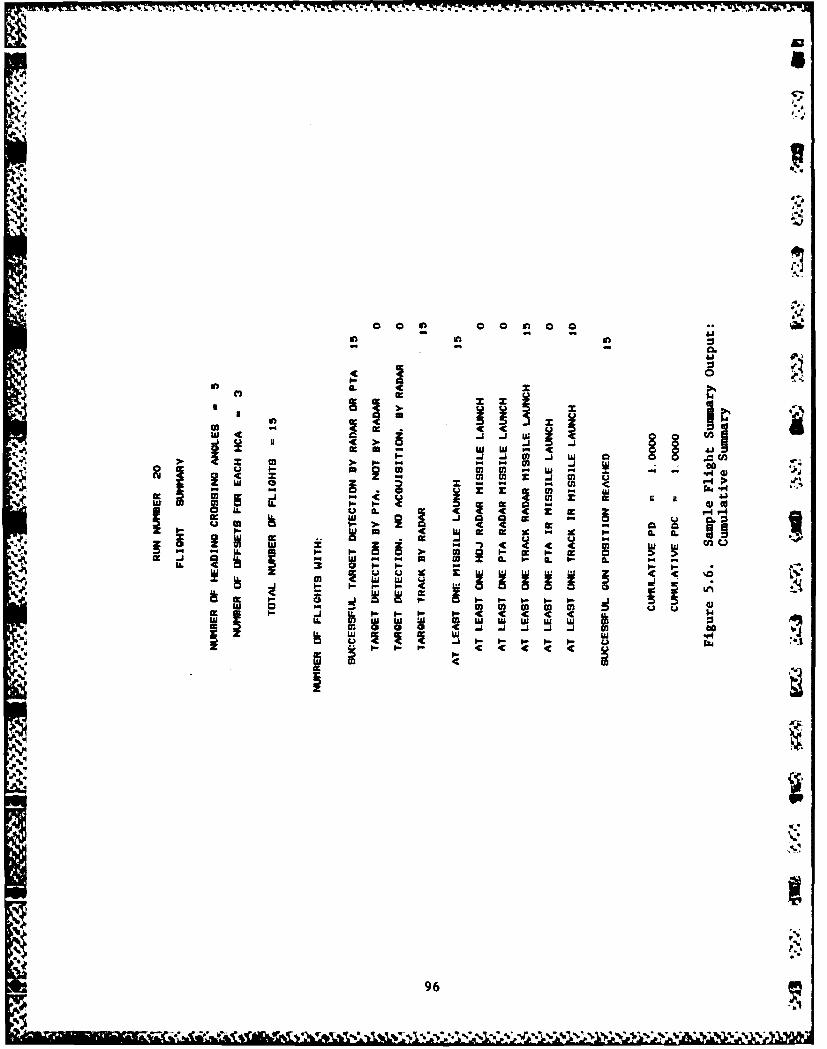
ENSS

00~0 0 0

--C I

> > 6-

j "q

cc -c 11 a

-. cc Ii 4 JcLL u IL C -C -C a _-

w 4 -C 0

fe jw -.- -C -C to

IL -

i igw 0 a m m

a j I- 4c -C -C -C $

LU LL4

w iLU i i0

96

-~I ~ ... . *. .& <b .AL&

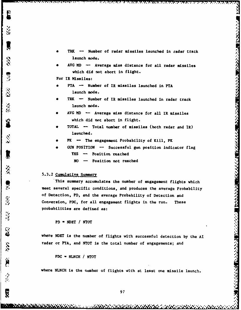
p

* TRK Number of radar missiles launched in cadar track

launch mode.

- 0 AVG MD - Average miss distance for all radar missiles 4.

which did not abort in flight.

For IR Missiles:

* PTA - Number of IR missiles launched in PTA

launch mode.

* TRK - Number of IR missiles launched in radar track

launch mode.

0 AVG MD - Average miss distance for all IR missiles

which did not abort in flight.

STOTAL - Total number of missiles (both radar and IR)

launched.

. PK - The engagement Probability of Kill, PK

* GUN POSITION - Successful gun position indicator flagYES -- Position reached

NO - Position not reached5.

5.3.2 Cumulative SummaryThis summary accumulates the number of engagement flights which

meet several specific conditions, and produces the average Probability

of Detection, PD, and the average Probability of Detection and

Conversion, PDC, for all engagement flights in the run. These

probabilities are defined as:

PD - NDET / NTOT

where NDET is the number of flights with successful detection by the AI

radar or PTA, and NTOT is the total number of engagements; and

PDC - NLNCH / NTOT

where NLNCH is the number of flights with at least one missile launch.

97*03. 0 -0 .i iJ 4 1

.45.4 FLIGHT PLOT FILE

This file contains the state of the AI, target, and each missile

launched in the engagement at each time step in the engagement. The

file can then be used by a post-processor to generate trajectory plots.

The state is an array of 10 elements containing:

* Time of the state

" X Position at this time

* Y Position at this time

" * Z Position at this time

4. * X-Dot (X-component of velocity) at this timeA. • Y-Dot (Y-component of velocity) at this time

0 Z-Dot (Y-component of velocity) at this time

%J 0 X-Double-Dot (X-component of acceleration) at this time

s Y-Double-Dot (Y-component of acceleration) at this time.4./ * Z-Double-Dot (Z-component of acceleration) at this time

The missile is identified by missile type (Radar or IR) and the

number of the missile (of this type).

The input variable IFLPLT is used to activate this output. Figure

5.7 provides a sample of this output.

5.5 DIAGNOSTICS FILE

Diagnostics can be generated by setting an input variable, KOUT.

This output is used for debugging and for tracing logic flow, time step

by time step. The resulting output file can be voluminous; it should be

used only for a single engagement. Some knowledge of the code is

required to decipher it since it references values by internal program

variable names. Each output line contains the routine name, dashes, the

program variable names, and their values. There are several levels of 4.

diagnostics available -- each adding to the last.

ioi7

98 I

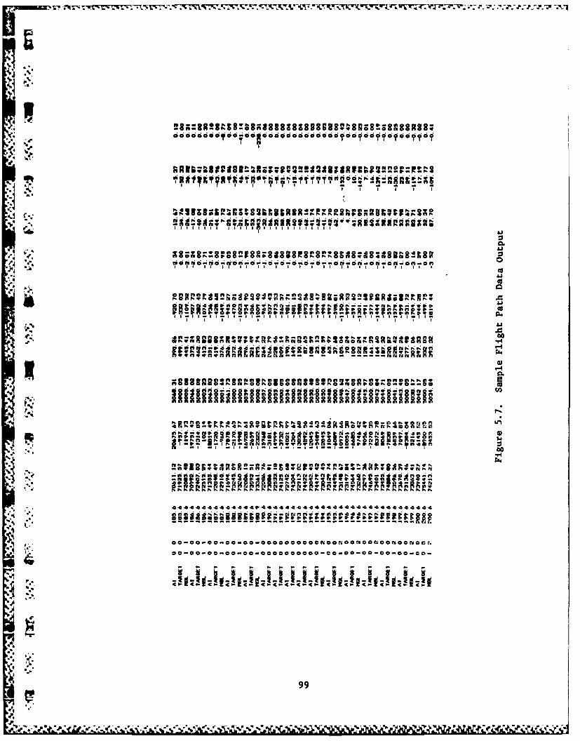
, I I I

t 'iii 4 tliid iii d ll . .. l .D . .I iIt I) I I I I

,w' . . . . . . ..1.1. . ...

i 'Sillllllilllillillill

00 0000--O0 O0 O0000000 O0 O-€Of0lO0 Oft

00 WO I0 f0 0 f0 0 0000000-0f 0-O VI-0N--00 -00--0

F00t-f~ -rg q~0I1N4 v0

6 .6Ws 1040 i l...Hqy In'

o

I'-

.99

KOUT Diagnostics:

0 No diagnostics generated

1 1 Minimal diagnostics at Event occurrences.*

2 Above plus AI and Target states and event failures.

3 Above plus Missile states.

In addition, this output file is used for the hard-copy option

available to the user when running the program. This option copies all

terminal input and output activity to a file. This is especially useful

when the user is working at a terminal screen and would like a printout

of the changes made~ during program execution. The first terminal input

requested by the program sets the hard-copy option. A sample of the

* output generated by this hard-copy option is provided in Fig 5.8.

100

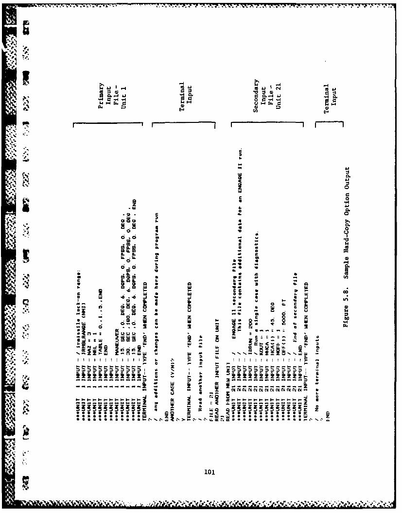
1-4- -~4J',) (P.J' tUjE I

0-4-4 00.-

'0V.

0.4 IL c

C 0

FA~

10 w 101

Vi APPENDIX A

RADAR DETECTION MODELS

Airborne radars can be classified by their ability to distinguish

target return signals from clutter (energy reflected from the ground).

The techniques employed to achieve this utilize the range and velocity

measuring capabilities of radar. Unfortunately, both range and velocity

cannot be measured simultaneously with the same degree of accuracy. To

a radar, time is the measure of range and frequency is the measure of

velocity. Since time and frequency have an inverse relationship, any

improvement In range measurement results in a reduction in the ability

to measure velocity on a single pulse. For this reason, all airborne

radars use information obtained by a long sequence of pulses. The rate

at which these pulses occur is called the PRF (pulse repetition fre-quency). The PRF determines the upper limits on the range and velocity

which can be measured unambiguously:

Unambiguous Range: R = (A--.1)U 2.-PRF

where c = speed of light

Unambiguous Velocity: V = (A.2)

.4'.. where X = wavelength . If the expected target ranges exceed R , ai • Uradar is said to be ambiguous in range, and similarly for velocity. AI

:, radars can then be classified as:

* Low PRF-Unambiguous in range but ambiguous in velocity.

• High PRF-Ambiguous in range, but unambiguous in velocity.

* Medium PRF--Ambiguous in both range and velocity.

PREVIOUS P AGV103 1s BLANKK

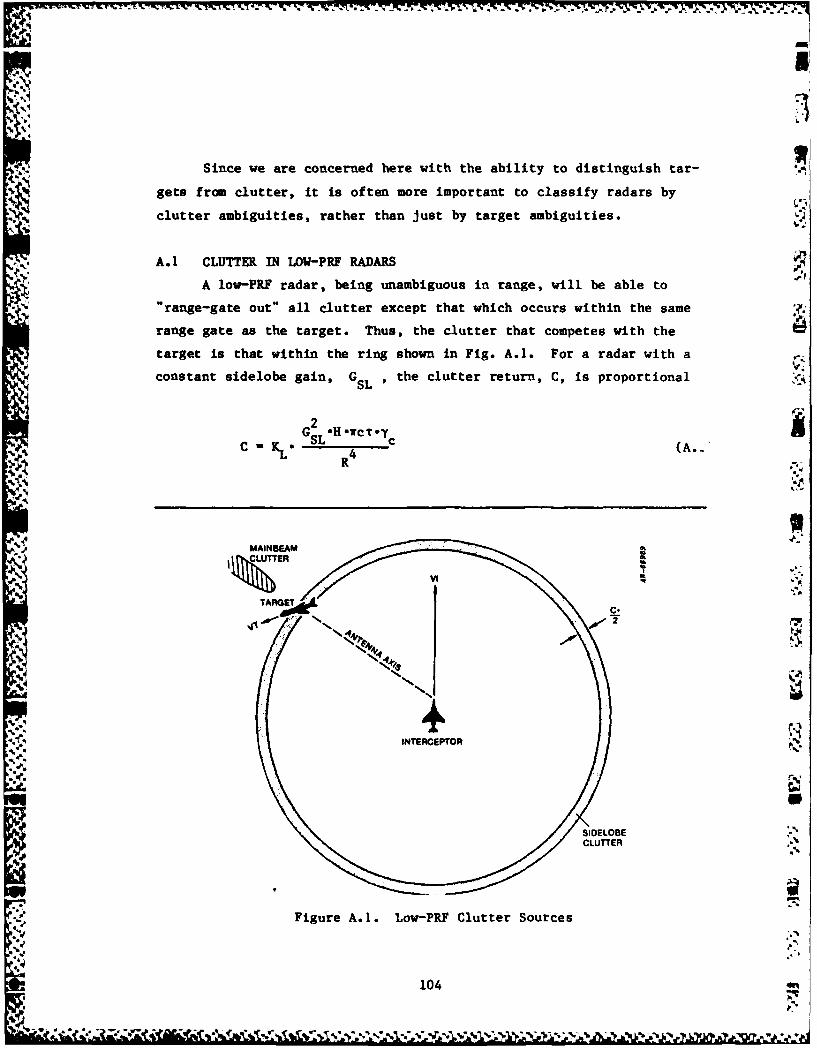
Since we are concerned here with the ability to distinguish tar-

gets from clutter, it is often more important to classify radars by

clutter ambiguities, rather than just by target ambiguities.

A.1 CLUTTER IN LOW-PRF RADARS

A low-PRF radar, being unambiguous in range, will be able to

* "range-gate out" all clutter except that which occurs within the same

range gate as the target. Thus, the clutter that competes with the

target is that within the ring shown in Fig. A.I. For a radar with a

constant sidelobe gain, GSL , the clutter return, C, is proportional

2G2SL .H .ircr*yc

C-K.. R c (A.

R

I

N "-N

Figure A.I. Low-PRF Clutter Sources

104

where Tr - pulsewidth• - clutter backscatter coefficient

H - altitude of radar

KL - constant

R - the range to the target

and the range gate is cT/2.

We're assuming here that the RCS of the clutter behaves as:

cc 'I sin erc

A where 8 is the grazing angle. If the mainbeam touches the ground,

GSL is replaced with GML , and the clutter return becomes enormous.

This accounts for the ineffectiveness of low-PRF radars in "look-down"

situations. If, in addition to range-gating, Doppler filtering is used,

an additional factor appears in Eq. A.1 to account for the fact that

some of the clutter in the ring of Fig. A.1 will not appear at the same

(ambiguous) velocity as the target. Typically, this clutter improvement

factor is --n the order of 2 to 5, and cannot overcome the mainbeam clut-

ter, if present.

A.2 CLUTTER IN HIGH-PRF RADARS

Since high-PRF radars are ambiguous in range, clutter returns from

a large number of range rings (Fig. A.2) will appear at the same time as

the target. However, only that clutter with Doppler return within a

bandwidth (B) of the target's Doppler will compete with the target sig-

nal. The total in-band clutter is the sum of all returns from the areas

(A i) of intersecting range rings and the isodop strip (so called because

it is bounded by curves of constant Doppler return). This is obviously

a very complicated function, but can be approximated by:

C %S~c (A.4)H 2 V

I.

105

Kh .sL-cU U -. ~ ~ " ~ "

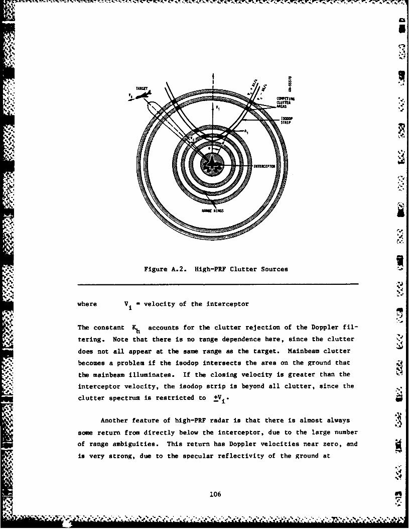
whreV t =CelctyoMtINntreGo

. 4•

rCLUTTER

,

clttr petFmigrestAic2e Hih-E ClttrVou. e

Anotherhre elocit of he inercetr sta thr isa otal ys

soeertg. No thtirey iseno tane denencere,e since thre nluteroes rnoteU apputer aTthesam range has thpetrgvelct.isneam cleranbecomesy ptrobldem if the isodpintersfectv theae on the ground at

t Re

clutterespectrum is restricted tources

soeretr fro decty bow the interceptor, u otelrenme

Thofanamitis acuts frtnhas Dopler ecities nftea zoper and-

iscovey strogle to the spla itrefectivtyae o the ground a

th4,nemilmnts.I h lsn eoit sgetrta h

106repo veoiy heqI- trpi eod l lter ic h

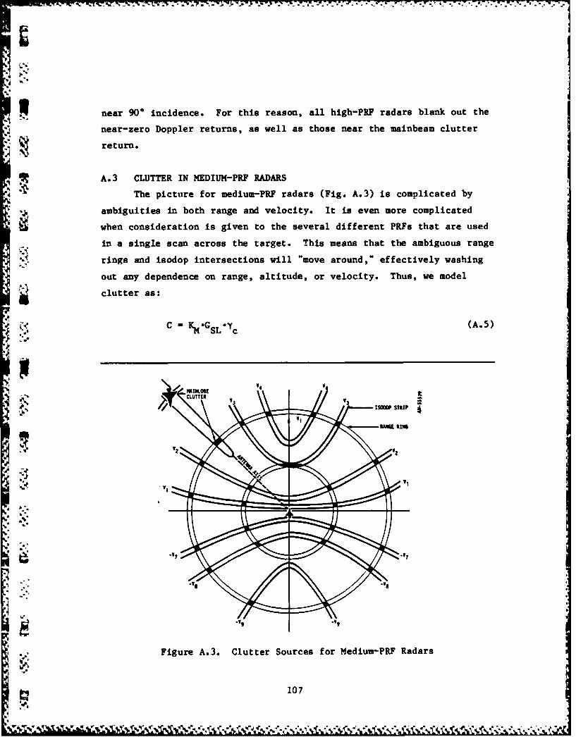
near 90 incidence. For this reason, all high-PR? radars blank out the

near-zero Doppler returns, as well as those near the mainbeam clutter

return.

S. A.3 CLUTTER IN MEDIUM-PRF RADARS

The picture for medium-PRF radars (Fig. A.3) is complicated by

ambiguities in both range and velocity. It is even more complicated

when consideration is given to the several different PRFs that are used

in a single scan across the target. This means that the ambiguous range

rings and isodop intersections will "move around," effectively washing

out any dependence on range, altitude, or velocity. Thus, we model

clutter as:

C KM*GSLOc (A.5)

4ONLB V V

"e" Figure A.3. Clutter Sources for Medium-PR? Radars

107

The constant KM here includes both clutter rejection and the averaging

effect of multiple PRFs.

Just as with the high-PRF radar, if the mainbeam clutter appears

- at the same Doppler velocity as the target, G SL is replaced with

G , and the signal-to-clutter ratio becomes very small. In addition,ML'it is possible for the mainbeam clutter to appear in an ambiguous

Doppler bin that matches the target. This is one of the reasons that

medium-PRF radars use several PRFs; to assure that some PRFs will be

able to resolve all targets except those whose (unambiguous) velocities

are within the mainbeam clutter. It is also possible for medium-PRF

radars to reject mainbeam clutter through range gating. This happens

only if the mainlobe clutter patch is shorter than the unambiguous range

(for example, in a very steep look-down). In practice, the mainlobe

clutter filters are blanked in all range gates, so real radars cannot

take advantage of this possibility.

A.4 SCALING EQUATIONS

We turn our attention now to the equations used in the simulation

and the data required to use them. The most common method used to spec-

ify radar performance is the range at which a specified cumulative

detection probability (usually 0.5 or 0.85) is achieved for a reference

RCS. Cumulative detection probability is given by:

- 1 - 1711 - PDSS(Ri) (A.6)i

where P " single scan probability of detection , and the product isDSS

taken over all scans across the target as range closes.

i "%"

For a Swerling I model of target RCS fluctuation: ".

Harold I. Jacobson, "Simple Formula for Radar Detection Probability onSwerling I Targets," IEEE Transactions on Aerospace and ElectronicSystems, March 1981, p. 304.

108

% . .. .......

PDSS "Pfa 1 s/I (A.7)

where P fa " probability of false alarm

and S/I - signal-to-interference power ratio

Since PCUM depends on how rapidly the range closes, it is not easy to

scale to conditions different from those under which it was derived.

It is more useful to specify a reference triplet of range, signal-

to-noise ratio and RCS (which we'll call R0, (S/N)., and co).

To understand why this is a useful approach, consider the follow-

ing form of the radar range equation:

R4 PTGX T (A.8))3(41) kTsFBN(.S)

The only factor that changes with range and RCS is (S/N) Using our

reference values, we can write:

R 00 (A.9)* 0 IS\

where we have lumped all constants into KO . At any other range and

RCS:

R S 0 a (A. 10)

0 0o1o

109

°q

km i .

So if we know any two values, we can solve for the other. For example:/s. ( FRN 0 .0 n_(A. 11)

If clutter is present, we are interested in determining the

signal-to-interference ratio:

ss'SS

I N + C (A.12)

As we have seen, determining the actual clutter power can be quite com-

plicated, so we once again resort to scaling. Assume we have a range

R1 Nat which our reference target (0 ) gives a S/I ratio equal to

(S/N)0 , but with clutter present. Then,

-) . .C. N (A.13)

N 0 1 N+C I+C/

But S/N at R is given by

R 4

So we can solve for C/N :

* Cin(= - I(A.15)

We require R1 < R , which means the radar cannot perform better

with clutter present than without. We can scale using:

110 .

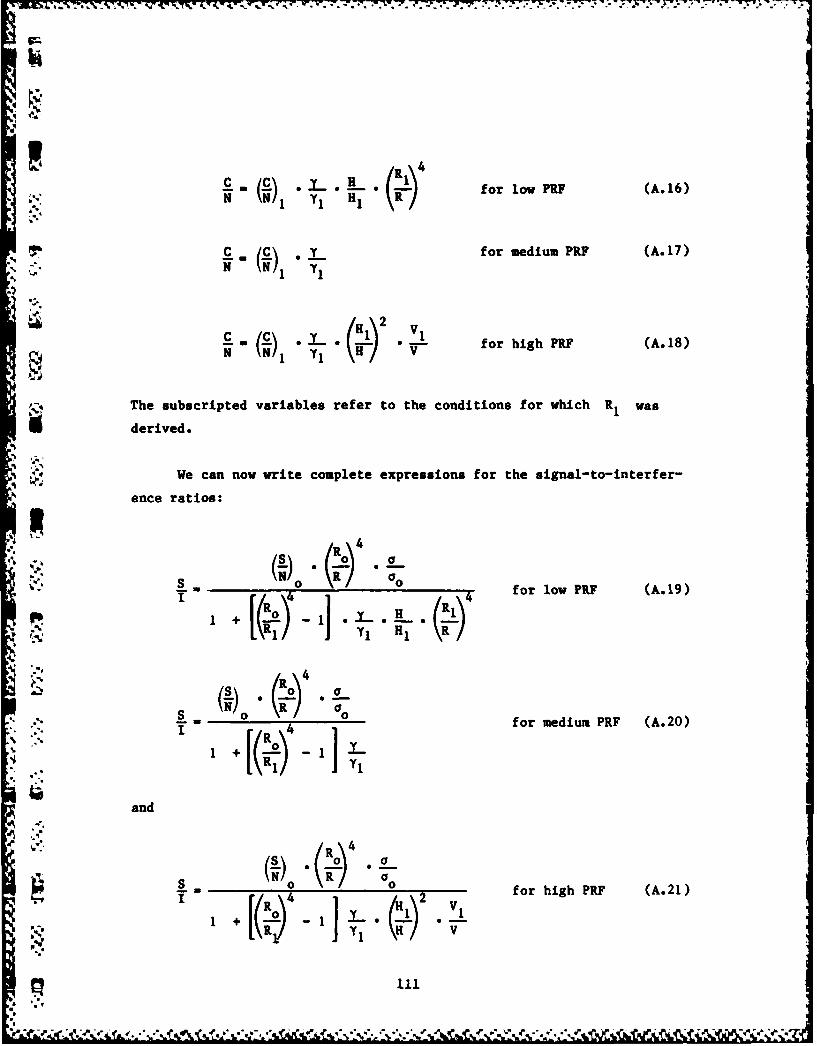
'9.'

N \N I _. a, \ for low PRF (A.16)

lC (C y' for medium PRF (A. 17)

N I Y

N (C) _ - - for high PRF (A.18)

The subscripted variables refer to the conditions for which R, was

derived.

We can now write complete expressions for the signal-to-interfer-

ence ratios:

+ 0 for low PRP (A.19)

I" + \% 1 -0 i _

., 4

0a

S 0 for medium PRF (A.20)

4[#4

I YI

and

So

_ _R _ 0 for high PRF (A.21)

1+

:. - +t -j, 7q

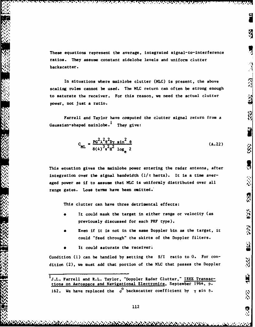
These equations represent the average, integrated signal-to-interference

ratios. They assume constant sidelobe levels and uniform clutter

backscatter.

In situations where mainlobe clutter (MLC) is present, the above

scaling rules cannot be used. The MLC return can often be strong enough

to saturate the receiver. For this reason, we need the actual clutter

power, not just a ratio.

Farrell and Taylor have computed the clutter signal return from a

Gaussian-shaped mainlobe. I They give:

;t MPG 2 )22Dy sin 2 (A.22)8(4)3w2H log e 2

This equation gives the mainlobe power entering the radar antenna, after

integration over the signal bandwidth (1/T hertz). It is a time aver-

aged power as if to assume that MLC is uniformly distributed over all

range gates. Loss terms have been omitted.

• 1 This clutter can have three detrimental effects:

p._ * It could mask the target in either range or velocity (as

previously discussed for each PRF type).

a Even if it is not in the same Doppler bin as the target, it

could "feed through" the skirts of the Doppler filters.

0 It could saturate the receiver. •U

o'.', Condition (1) can be handled by setting the S/I ratio to 0. For con-

dition (2), we must add that portion of the MLC that passes the Doppler

IJ.L. Farrell and R.L. Taylor, "Doppler Radar Clutter," IEEE Transac-tions on Aerospace and Navigational Electronics, September 1964, p.

162. We have replaced the a backscatter coefficient by y sin e.

112

' " 'M " • % *

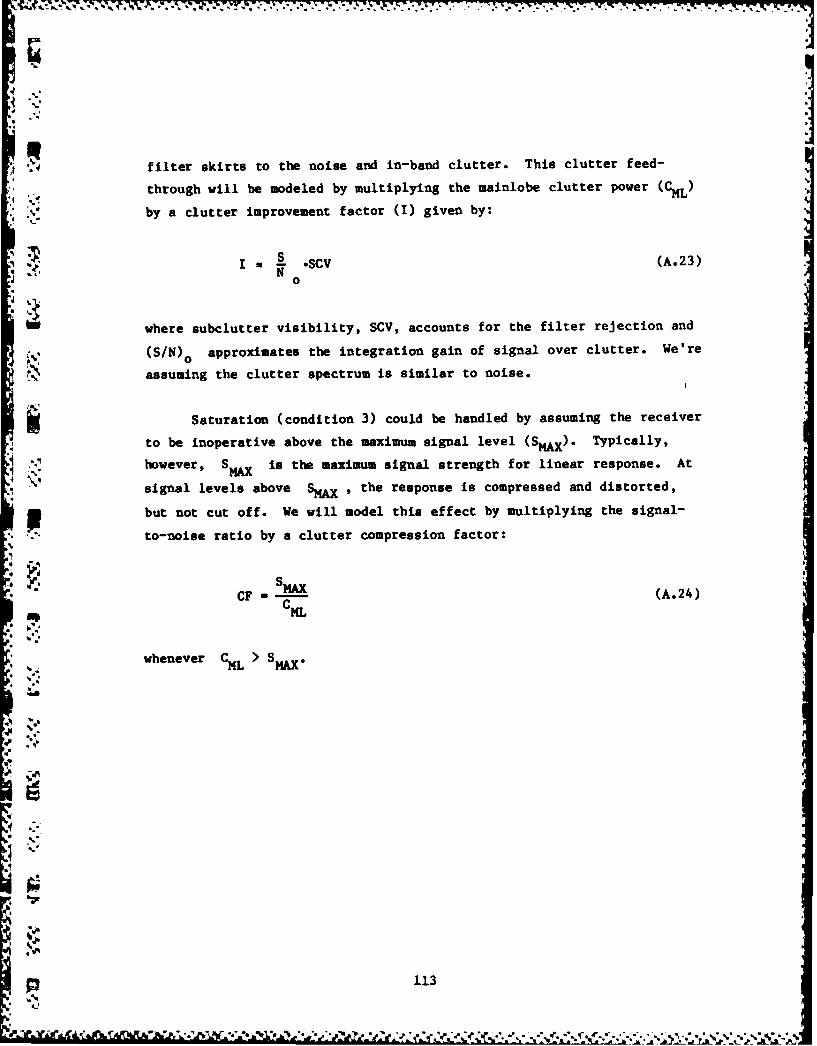
A 'filter skirts to the noise and in-band clutter. This clutter feed-

through will be modeled by multiplying the mainlobe clutter power (CML)

by a clutter improvement factor (M) given by:

0- .SCV (A.23)

Wwhere subclutter visibility, SCV, accounts for the filter rejection and0O

(S/N)o approximates the integration gain of signal over clutter. We're

assuming the clutter spectrum is similar to noise.

ISaturation (condition 3) could be handled by assuming the receiver

to be inoperative above the maximum signal level (SMAX). Typically,

. however, SMAX is the maximum signal strength for linear response. At

signal levels above SMAX , the response is compressed and distorted,

but not cut off. We will model this effect by multiplying the signal-

to-noise ratio by a clutter compression factor:

S ACF, , = - (A.24)

whenever CML > SMA .

,

p 113

-~ .:..

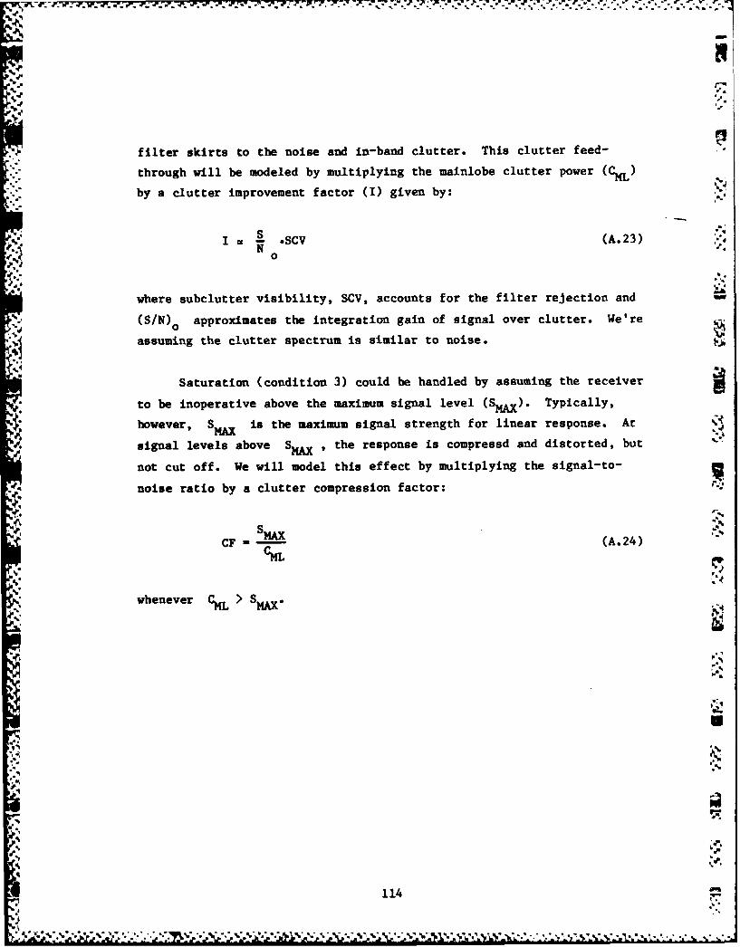
NNI0 filter skirts to the noise and in-band clutter. This clutter feed-

Sathrough will be modeled by multiplying the mainlobe clutter power (CML)

Sby a clutter improvement factor (I) given by: (i

.

MAX4

where subclutter visibility, SCV, accounts for the filter rejection and

(S/N) o approximates the integration gain of signal over clutter. We're

assuming the clutter spectrum is similar to noise.

Saturation (condition 3) could be handled by assuming the receiver

* to be inoperative above the maximum signal level (SM~x). Typically,

however, SMA is the maximum signal strength for linear response. At 9

signal levels above SMAX , the response is compressd and distorted, but

not cut off. We will model this effect by multiplying the signal-to-

noise ratio by a clutter compression factor:

,..

CF - -- (A.24)

CML

whenever CML > SIM

A1,1

•.4.

APPENDIX B

JAMING

Three types of jamming are modeled by ENGAGE II:

a Noise jamming, which is assumed to be continuous in time

(cv).

, Track break jamming, a responsive technique that denies

acquisition.

a Deceptive countermeasures (DEC4), which cause errors in

range or angle measurement.

All three types of Jamming are characterized by the effective radiated

power (ERP) and bandwidth (BWJ). Since ERP includes the jamumer's

antenna gain, it is input as a function of the aspect angles (azimuth

and elevation) of the target. BWJ is assumed to be greater than the AI

? 'radar bandwidth. Since ENGAGE II is a one-on-one model, all jamming is

considered to be in the mainlobe.

The Jammer's effects on the radar receiver are dependent on the

J/N power ratio:

~ yJ -ERP GRX 2BL )I % " BWJ 2 kTsF (B.1)

where GR w radar mainlobe antenna gain

R - range to Jammer

Lj antenna to receiver losses

k - Boltzmann' s constant (1.38 x 10 Joule/*K)

T 8 - effective system temperature

' e 115

~m.4

4r-.

FN =receiver noise figure

X RF wavelength

The term is a lumped loss term, and should include antenna, wave-

guide, and amplifier losses. Any processing gain for the target signal

(such as coherent integration) should also be included in Li . Typi-

cally, Lj is much less than one. T is assumed to be 290*K.

Noise Jamming is assumed to add directly to noise and clutter,

giving a total signal-to-interference ratio of

I N+C+J (B.3)

f9

Signal-to-jamming power is given by:

S " S N (B.4)

|o.

where S/N is computed as described in Appendix A. The S/I ratio is

used to compute the single-scan detection probability:

I + S/7DSS FA (B.5)

And to determine if tracking is possible:

s- > ACRIT (B.6)

where ACRIT is the threshold tracking level.

116

i..' If the AI radar has the ability to track-on-Jam, a second thresh-

old (TTOJ) is used with the J/N ratio:

%

J> TTOJ (B.7)

When this condition occurs, the radar is assumed to track in angles

only, not in range. Note that it is possible for both inequalities of

Eqs. B.6 and B.7 to be satisfied. When this occurs, normal radar track-

ing takes precedence over track-on-jam.

Track break and deceptive jammers must capture the receiver in

order to be effective. This is modeled by setting a "Jammer effect-

iveness ratio," TJEFF . The AI radar is assumed to operate normally as

'4 long as:

< T JEFF (B.8)

-S If the inequality in Eq. B.8 is not satisfied, a track break jam-

mer wil prevent acquisition until burnthrough. No track-on-jam capa-

bility is assumed for this type of jamming.4

DECK is also considered to be effective when J/S > T J In

this case, bias error terms are added to the range, azimuth, and/or ele-

, 0' vation angles to the target. These errors impact the missile launchcalculations and the Al maneuver instructions, which will be discussed

in the next two appendices.

4.

117

,- - , . .' '"

."

' " " - .,.. ,.- , , . - - - - . ,

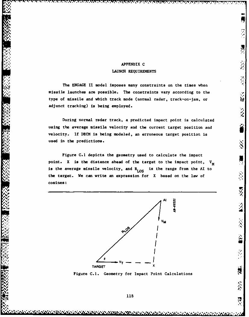
APPENDIX C

LAUNCH REQU IREMENTS

The ENGAGE II model imposes many constraints on the times when

missile launches are possible. The constraints vary according to the

type of missile and which track mode (normal radar, track-on-jam, or

adjunct tracking) is being employed.

During normal radar track, a predicted impact point is calculated

using the average missile velocity and the current target position and

*velocity. If DECH is being modeled, an erroneous target position is

used in the predictions.

Figure C.1 depicts the geometry used to calculate the impact

point. X is the distance ahead of the target to the impact point, V,

is the average missile velocity, and ROS is the range from the Al to

the target. We can write an expression for X based on the law of4°

cosines:

_-... v..*. J. Al

VM

*... I :

TARGET X

Figure C.1. Geometry for Impact Point Calculations

~118

a.%.

Sle

X R

-LOS + (c.1)

where

VM

SVT

The negative root is of no interest (it corresponds to negative

flight time). In most cases, the missile velocity is not constant. For

this reason, a two-step iteration is used to refine the estimate of

average velocity. The first step uses the AI velocity to calculate an

impact point (earliest collision point on target path which AI can

reach). The range from the AI to this point is used to estimate the

average missile speed. This speed is then used to find a second impact

point, which is used to calculate the range to impact and the heading

Verror (angle between the AI velocity vector and the line-of-sight vector

to the impact point).

The following checks are made to determine if a missile launch is

possible:

-" The range to impact must be greater than the input minimum

range and less than the maximum range.? ".'

• The heading error must be less than the input maximum.

" a The velocity at impact must be greater than the target

velocity.

, ,The current AI acceleration must be less than the input max-

imum g-limit.

Additional criteria are imposed depending on the type of missile:

0 IR missiles must be within the aspect dependent lock-on

range.

119A-

W~ - ~ * *.~ .~ V N

Semi-active (LOBL) missiles must have seeker lock-on.

* No additional checks are made for active (LOAL) missiles,

but they must achieve lock-on during flight before an input

time limit prior to impact.

Seeker lock-on for all three types of missiles includes gimbal

limit checks. EF missiles (both active and semi-active) require the

signal- to- interference ratio (see Appendices A and B) to be greater than

* an input threshold.

Only RF missiles can be launched if the AI radar is tracking on

noise jamming. In this mode, no impact predictions are made, since the

radar is presumed to have no range or range rate data. Only three

checks are made:

0 The heading error (which in this case is the angle between

the AI velocity vector and the jam strobe) is less than the

allowed heading error.

0 The current AI acceleration is less than the maximum

allowed.

0 The missile (either active or semi-active RF) has a home-on-

jam capability and the J/N ratio exceeds an input threshold

level.

Since no checks are made on range or velocity, it is quite possible for

missiles to be launched which have no chance of reaching the target.

Missile launches using the passive track adjunct mode are very

similar to normal radar track launches. Since the track adjunct is

assumed to have no Doppler measurement, no prediction is used. Instead,

4 the current target position is used to determine if the target is within

missile reach. Semi-active missile launches are not allowed during

* adjunct tracking since they require radar illumination.

120

P " L%

" " : " " ' " " : "". ..

APPENDIX D

AI MANEUVERS

During the course of any air-to-air engagement, the interceptor

. . may be required to perform several types of maneuvers. Since ENGAGE II

* does not include a reactive target, no "dog-fighting" is modeled. Thus,

the list of required maneuvers can be limited to:

, Direct Pursuit-in which the AI flies directly toward the

target. This maneuver is used during track-on-jam and

adjunct tracking.

a Lead Pursuit-in which the AI flies toward a predicted

impact point ahead of the target. This maneuver is used

during normal radar track.

0 0 Breakaway-in which the AI flies toward an offset position

in order to convert to a stern attack.

. Tail Chase-in which the AI attempts to achieve a position

to launch rear-hemisphere (IR) missiles or to fire guns.4. .. '

All four types of maneuvers are in some way related to the target

S" kposition. Prior to acquiring the target, no maneuvers are allowed.

Maneuver instructions are generated in a two-step process:

a An aimpoint is calculated.

. Heading changes necessary to align the AI velocity vector% with the aimpoint are calculated.

We'll first discuss how the aimpoints are calculated for the four

* -..o maneuvers*

The aimpoint for direct pursuit is Just the current target

position.

121

The aimpoint for lead pursuit is determined as described in

Appendix C for any remaining missiles. If no impact point can be

found-as can happen if the missile velocity is too low-the aimpoint

calculated using the AI velocity is used for maneuvers. The missile

launch priority (an input) is used to select either the IR or RF

aimpoint.

The aimpoint used for breakaway is offset from the target by a

distance equal to the AI's turn diameter, and behind the target by the

1% desired tail chase position. This maneuver is only used when:

• The AI is in front of the target, and

• No missiles with forward hemisphere capability are left

The breakaway continues until a position has been reached from which the

AI can turn to the target's stern. This occurs when:

A m R.cos(O) + V1 sin(A) + RT (D.1)

TR TR

where A angle through which AI must turn

VT = target velocity

.J..: T R AI turn rate (radians/sec)

R -range from AI to target

S-aspect angle from target to AI

r - desired distance behind target

V M Interceptor Velocity

Figure D.1 shows some of the variables in Eq. D.1. The term

A.VT/TR is the distance the target will move while the AI is turning

through the angle A . R cos(e) is the distance the AI is ahead of the

target. V I/T RSin(A) is the distance along the target's velocity

vector the Al will move during the turn.

122

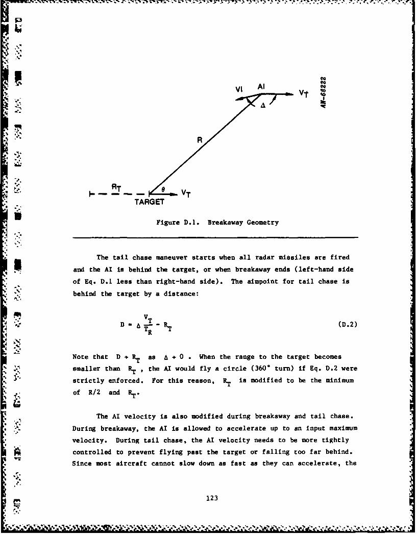
i -,r

TARGET

Figure D.1. Breakaway Geometry

* The tail chase maneuver starts when all radar missiles are fired

Sand the AI is behind the target, or when breakaway ends (left-hand side

of Eq. D.1 less than right-hand side). The aimpoint for tail chase is

*behind the target by a distance:

VT R (D.2)TR

Note that D + * as A +. 0 . When the range to the target becomes

smaller than RT , the AI would fly a circle (3600 turn) if Eq. D.2 were.*,* strictly enforced. For this reason, R.T is modified to be the minimum

of R/2 and T

The AI velocity is also modified during breakaway and tail chase.

During breakaway, the AI is allowed to accelerate up to an input maximum

velocity. During tail chase, the AI velocity needs to be more tightly

controlled to prevent flying past the target or falling too far behind.

Since most aircraft cannot slow down as fast as they can accelerate, the

123

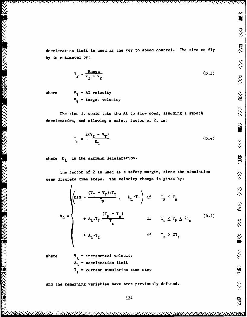
' - ' . .. . '- : , ... *. .'.i .' . * % . . 4.. ,.t., .°J .,. . -.-

deceleration limit is used as the key to speed control. The time to fly

by is estimated by:

Range (D.3)TF =V I - VT

I T

where VI = AI velocity -V

VT =target velocity

The time it would take the AI to slow down, assuming a smooth

deceleration, and allowing a safety factor of 2, is:

T - 2(VI - VT) (D.4)s DL

where DL is the maximum deceleration.

The factor of 2 is used as a safety margin, since the simulation

uses discrete time steps. The velocity change is given by:

MIN T T I DL T if TF < TM TF I).

V A = i (TF - Ts)(D5& AL.T I T if Ts < TF < 2T (D.5)

+AL.TI if TF > 2T sU

where V M incremental velocity

AL - acceleration limit

T M current simulation time step

and the remaining variables have been previously defined.

124

" ,.V. .;' "."'; % - ' "/. ' 4 / '.* -'t -'.* *..* *.o-* . -.- -,.-." . " . " '" '" "-f t . .". f.t "V' ' '

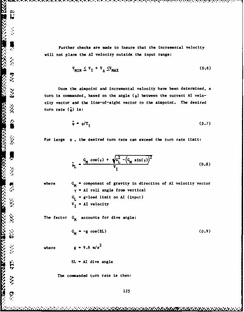
- Further checks are made to insure that the incremental velocity

will not place the AI velocity outside the input range:

VMI N < VI + V <VMA X (D.6)

:I tu n Once the aimpoint and incremental velocity have been determined, a

turn is commanded, based on the angle (*) between the current AI velo-

- city vector and the line-of-sight vector to the aimpoint. The desired

turn rate (,) is:

-*/T I (D.7)

, For large , the desired turn rate can exceed the turn rate limit:

Ghee Cs (: + ((D.8)

where Gt - component of gravity in direction of AI velocity vector

y - AI roll angle from vertical

GL - g-load limit on AI (input)

V . AI velocity

" The factor GM accounts for dive angle:

G - -g cos(EL) (D.9)g 9

U. " where g = 9.8 m/s2

EL AI dive angle

_ The commanded turn rate is then:

125

". 5

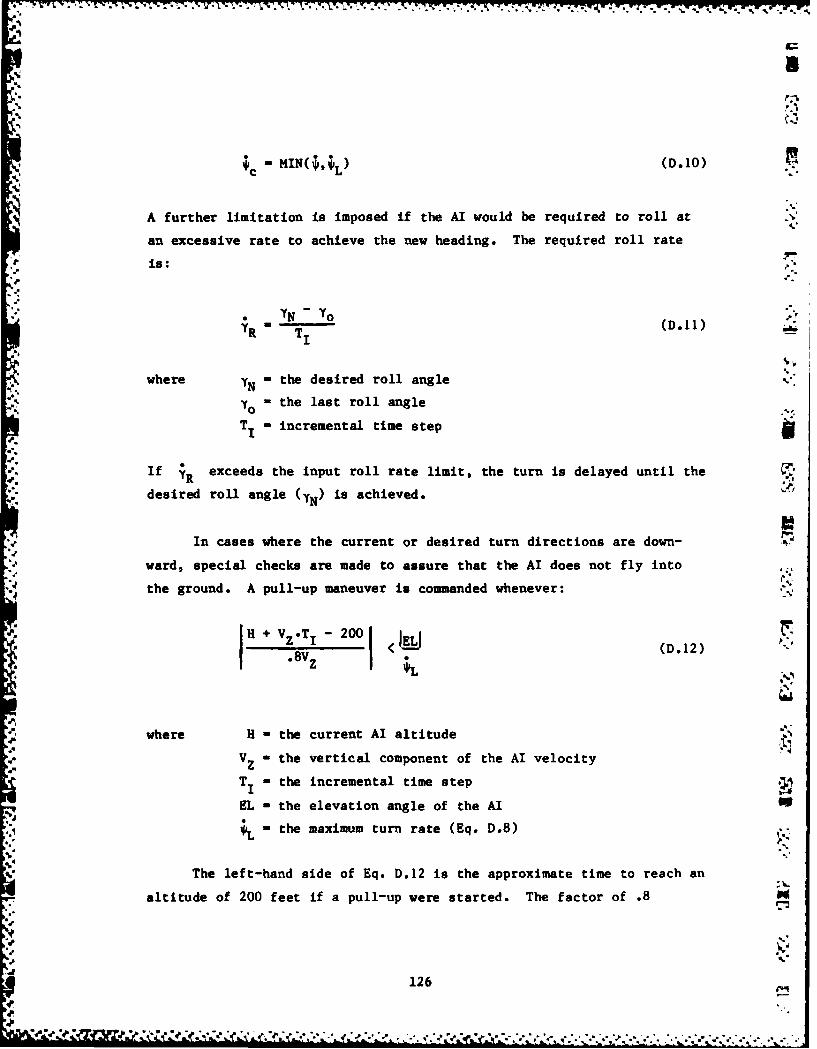
p.

S c MIN(,L) (D.10)

A further limitation is imposed if the AI would be required to roll at

an excessive rate to achieve the new heading. The required roll rate

is:,. _.

iR T I (D.11)

where YN the desired roll angle

Yo the last roll angle

TI incremental time step

If R exceeds the input roll rate limit, the turn is delayed until the

desired roll angle (yN) is achieved.

In cases where the current or desired turn directions are down-

ward, special checks are made to assure that the AI does not fly into

the ground. A pull-up maneuver is commanded whenever: ,

H + VzT 1 - 200 __ (D.12)p

8V (1"*L

where H the current AI altitudeV z the vertical component of the AI velocity

T - the incremental time step

EL -the elevation angle of the AI

- the maximum turn rate (Eq. D.8);.

The left-hand side of Eq. D.12 is the approximate time to reach an

altitude of 200 feet if a pull-up were started. The factor of .8 -

126 5.'

'..

"4 #',,/ /.7r / /;, e",;, .' e' . ,"., ,- ,,,-~ ~ .AA • . .*,*,. .*,* .. ... •. , ,.,- • .. *.* .

accounts for the reduction in vertical velocity as the pull-up is incre-

mented. The term EL/ is the approximate time it would take toN;'

change the elevation angle from EL to zero.

Before each new maneuver is implemented, another check is made to

make sure the new maneuver will allow the Al time to pull up later.

This check uses the same form as Eq. D.12 with V~ replaced vith the

estimate of the vertical velocity after the new maneuver and EL with

an estimate of the new dive angle.

Once the maneuver direction, turn rate, and speed acceleration

have been determined, the AI trajectory is updated using the same

equations of motion as for target maneuvers as described in Appendix G.

.12

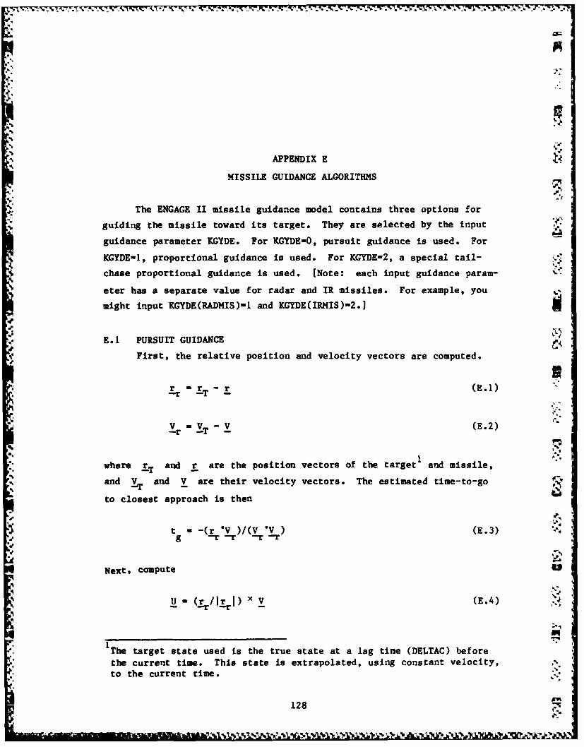
APPENDIX E

MISSILE GUIDANCE ALGORITHMS

The ENGAGE II missile guidance model contains three options for

guiding the missile toward its target. They are selected by the input

guidance parameter KGYDE. For KGYDE=O, pursuit guidance is used. For

KGYDE-1, proportional guidance is used. For KGYDE-2, a special tail-

chase proportional guidance is used. [Note: each input guidance param-

eter has a separate value for radar and IR missiles. For example, you

might input KGYDE(RADMIS)-1 and KGYDE(IRMIS)-2.]

E.1 PURSUIT GUIDANCE

First, the relative position and velocity vectors are computed.

r r =E -r (E.1)

Vr -yT - V (E.2)

"where rT and r are the position vectors of the targetand missile,

and V and V are their velocity vectors. The estimated time-to-go

to closest approach is then

t - -(r .V )/(V *V (E.3)"d g -- -r -r --

Next, compute

U - (r /ir I) x V (E.4)-r -r

The target state used is the true state at a lag time (DELTAC) before

the current time. This state is extrapolated, using constant velocity,

to the current time.

128

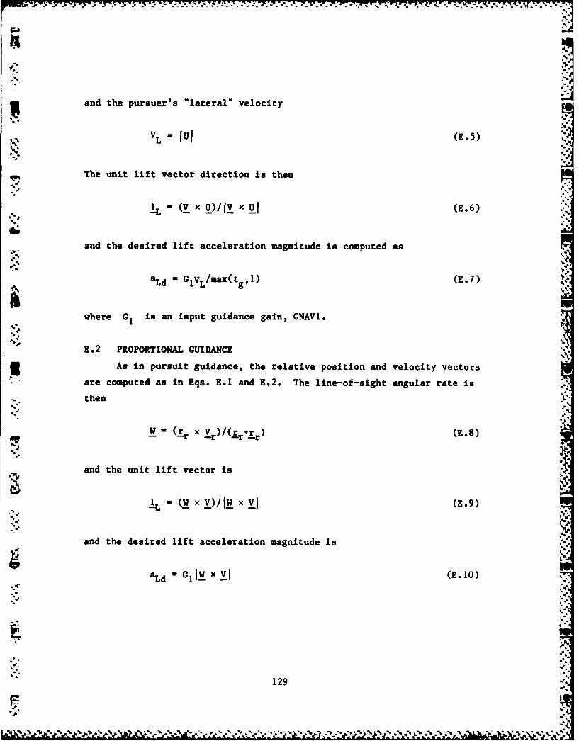
and the pursuer's "lateral" velocity

VL - lul (E.5)

The unit lift vector direction is then-V

.- - (V x u)/Iv x u (E.6)

and the desired lift acceleration magnitude is computed as

aLd - GiVL/max(tgV1) (E.7)

where G1 is an input guidance gain, GNAV1.

E.2 PROPORTIONAL GUIDANCE

3As in pursuit guidance, the relative position and velocity vectors

are computed as in Eqs. E.1 and E.2. The line-of-sight angular rate is

. then

0U - (rr X (Er) (-r) (E.8)

and the unit lift vector is

- (W x V)/i_ xvl (E.9)

.41

and the desired lift acceleration magnitude is

8 Ld = G l ! x V I (E.1O)

" 12

a 129

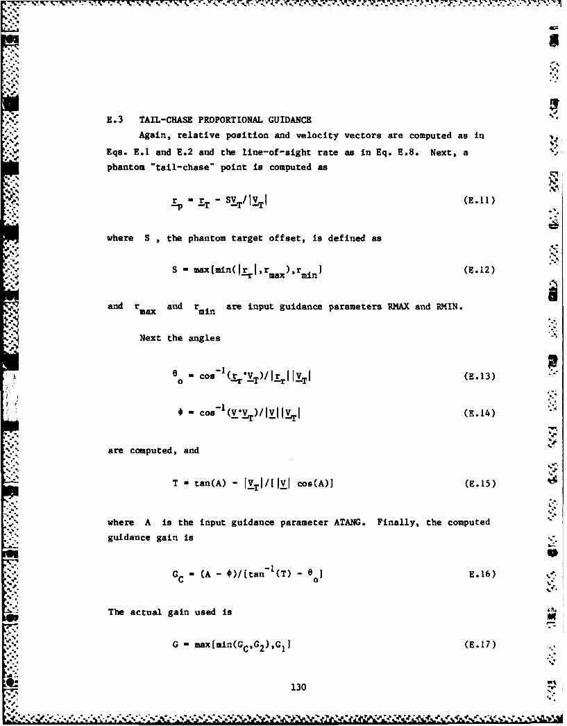
(e.

E . 3 TAIL-CHASE PROPORTIONAL GUIDANCE

Again, relative position and velocity vectors are computed as in

Eqs. E.1 and E.2 and the line-of-sight rate as in Eq. E.8. Next, a

phantom "tail-chase" point is computed as

r p - r - SVT/I VT (E.11)

where S ,the phantom target offset, is defined as

S - max[min( Ir T,r max),rmi n ) (E.12)

and rmax and rmin are input guidance parameters RMAX and RMIN.

Next the angles

80 " cos- 'v3 )/ I-r TI (E.13)

).US-cos -1 (V "vT) 13v I VTI (E.14) "

are computed, and

T- tan(A) -lVTI/[II cos(A)J (E.15)

where A is the input guidance parameter ATANG. Finally, the computed

guidance gain is

GC =(A - )/[tan- (T) - I E.16)

The actual gain used is 'S.

G - max[min(GC,G2 ),G1 ] (E.17)

'2: 130

mp

IF

,N where G and G are the input guidance parameters GNAV1 and GNAV2.1 2

The unit lift vector Is given by Eq. E.9 and the desired lift accelera-

tion magnitude is

aLd - GW x VI (E.18)

Cot.

131"

I 1" ;C.'

!::::1.31.

F-7.

APPENDIX F

MISSILE EQUATIONS OF MOTION

The point-mass model employed in ENGAGE II for the missile's

flight dynamics includes aerodynamic, gravitational, and rocket thrust

forces, a time-varying mass, and provision for up to seven stages. The

model requires the following input parameters for each stage to

physically describe the missile:

* Initial vacuum thrust T (CPTHRST)

. Initial weight Wo (CPMASSI)0 Final weight Wf (CPMASSF)

. Burn time tb (CPTB)

* Nozzle exit area A (CPNEA)e

* Aerodynamic reference area A (CPAREA) .

. Either

Cone angle 9c (CPCONE) and induced axial force coef-

ficient C (CX2CP), to compute the axial forcex2

coefficient C x by functional expression

* Or, alternatively,

A table for powered flight (CXCPKB)1 and, if applic-

able, for coasting flight (CXCPKC), or C as afunction of Mach number M and angle of attack a

IThe letter K in these tables represents the digit 1, 2, ., 7 cor-responding to the stage number.

132

U. Either

Normal force coefficients C (CNICP) and CN

N1 2(CN2CP) to compute the normal force CN as a quadra-

tic expression in a

• Or, alternatively,

A table (CNCPK)1 of CN as a function of M and a

* Coast time before ignition (TCOB4I) and after burnout

(TCOABO)

0 Maximum permissible normal acceleration loading aNmax

(ANMAXCP)

f Maximum angle-of-attack a (ALFMXCP),, max

Each of the foregoing input parameters will have separate tables

for each missile type (RABKIS or IR1I4S).

Figure F.1 shows the aerodynamic and thrust acceleration vectors

used in the model.

The missile's equations of motion are

- v (F.1) f-.

- a v + aLIL + (F.2)

In these equations, r, v , and a are the missile's position, velocity

and acceleration vectors, respectively; 1v and 11L are unit vectors

The letter K in these tables represents the digit 1, 2, ... , 7 cor-responding to the stage number.

133

AAo ALAf "t.. f * 't f ' * *

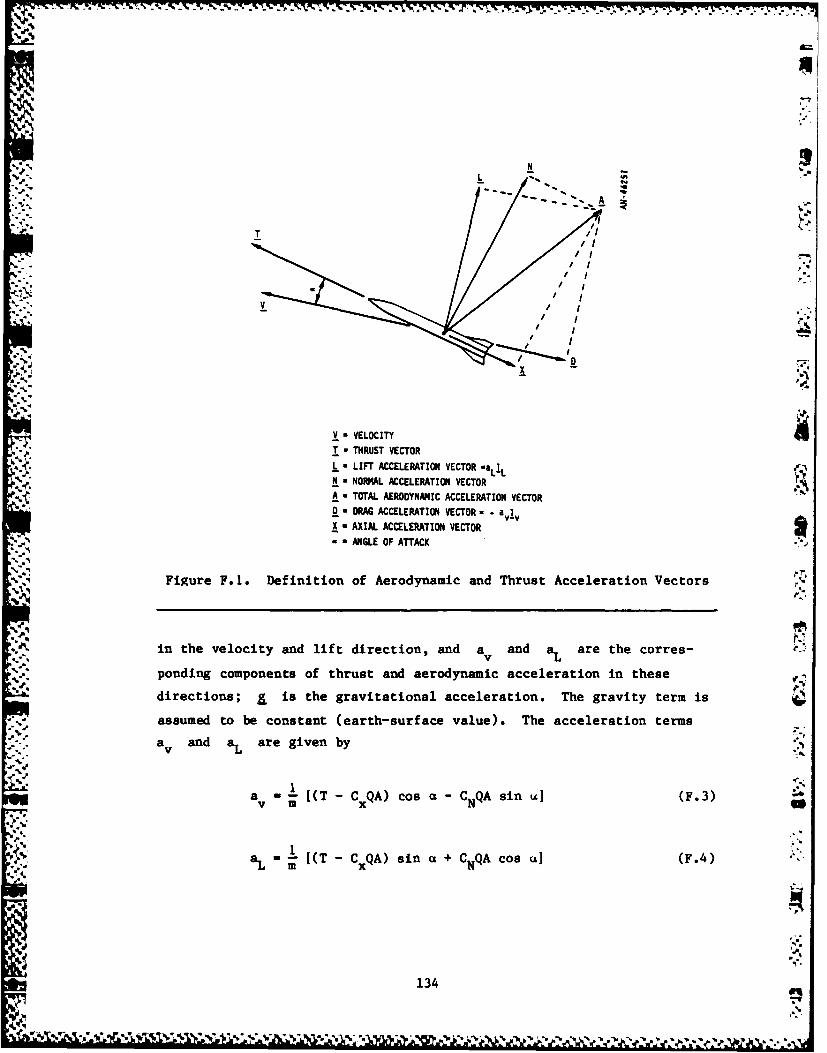
AA

T ,

D /7

I VELOCITYI-THRUST VECTOR

*LIFT ACCELERATION VECTOR aIN * NORMAL ACCELERATION VECTOR

-. TOTAL AERODYNAMIC ACCELERATION VECTOR

- B RAG ACCELERATION VECTOR - - av1vAXIAL ACCELERATION VECTOR

- 9 AN L O.TT C

Figure F.1. Definition of Aerodynamic and Thrust Acceleration Vectors

in the velocity and lift direction, and a v and aL are the corres- e

* ~. ponding components of thrust and aerodynamic acceleration in thesedirections; & is the gravitational acceleration. The gravity term is

assumed to be constant (earth-surface value). The acceleration terms

a and aL are given by

x N

al m - [T -CxQA) sn a + CN QA cs uJ (F.4)

13

A-~ ~~~~~~~_ AL ((CAsnICQcs J(F

where T is the delivered thrust; Cx and CN are the axial and nor-

mal aerodynamic force coefficients; Q , the dynamic pressure, is given

• ,by

2Q -=-- (F.5)

where P is the atmospheric density, computed as a piecewise exponen-

tial function of the missile's altitude; and m is the current mass of

the missile.

Two alternative models for the thrust profile are available in the

M program. The first assumes constant vacuum thrust for the duration of

the stage burn time:

T T0 (F.6)

The second model (selected by input of the initial thrust CPTHRST as a i',

negative value) assumes a decreasing vacuum thrust shaped to yield

constant axial acceleration:

(t-t )/tb

T•- T(f (F.7)vac W/

where ti is the ignition time of the current stage. The delivered

thrust is then obtained from the vacuum thrust by the expression

T -Tva -PA (F.8)vac

where p is the atmospheric pressure corresponding to the missile's

altitude, computed as

4wr

135

• b °

C~ C * ? ~ *

=%=

2p (F.9)

Y

where c is the local velocity of sound, a piecewise linear function of

the missile's altitude, g is the gravitational constant, and y the

gas ratio of specific heats (1.401). During coasting periods, of

course, T - 0.

The missile's mass m is computed according to one of two formu-

las, depending on which form of thrust calculation is being employed.

For the constant thrust model, mass decreases linearly with time:

M = [W - (U0 - wf)("t t) (F.10)

For the variable thrust model,

(t-t I)/t b

M Z%) (F.11)

During coasting, m remains constant at W /g or Wf/g for pre-ignition or post-burnout coasts, respectively.

The aerodynamic coefficients C and CN are generally expressed

as functions of M and a, where the Mach number M is obtained fromthe missile's velocity by the relation p.

M - (F.12)

Either or both of these functions may be input to the prog- n In tabular

form. If not so input, functional expressions will be employed. The

136

ft .

expression for C represents a simplified theoretical model for the

axial force coefficient of a cone:

2 sin 2 e +C a2 M <0.5c x2

2 0.3125 + 1.118 sin

JI2sin 2 0 1. + 1.1 i c 0.4444k__ec + 0.0625 + 1.118 sin c 1. + 2 sin 2 0 -/ 0.5),

L \ s n

C- +C 2 ; 0.5 <M < 1.5

2 /0.3125 + /T ie\ k 22.sin + si+ Cx2 ; > 1.5c 00625 + ;M-1sin M 2

(F.13)

where k - 0 during powered flight, and k - 1 during coasting flight.

The expression for CN is a quadratic in 0:

C- Ca + C 2 a2 (P.14)N =N N (.4

The angle of attack a is taken to be the smallest of the follow-

ing three quantities: (1) commanded angle-of-attack, ac ; (2) limiting

angle of attack, a ; and (3) angle-of-attack, a , yieldingmax Nmax

limiting normal acceleration, aNmax ; as computed by iteratively solv-

ing the implicit equation

I."

a C N (aax (F.15)Nmax m

for a

137

'.1*

r,- ,* -

The commanded angle-of-attack is obtained by iteratively solving

the equation

a OA [CN(M'ac) cos ac - Cx(M,ac) sin ac] (F.16)

for ac . Here, aLA is the desired aerodynamic lift acceleration. It

is computed from the desired total lift acceleration aLd by

aLAaLd-Ig --L (F.17)

where aLd is computed by the guidance algorithm and I is zero if

the input guidance parameter INCLG is zero or negative, and Ig is one

otherwise.

The unit lift vector, IL , is computed by the guidance algorithm.

Equations F.1 and F.2 are numerically integrated using fourth-

order Runge-Kutta integration with a time-step specified by the input

parameter DTINT. Integration is terminated at each dynamic discontinu-

ity (such as staging, burnout, or target-closest-approach) and, if

appropriate, restarted after the discontinuity.

The missile trajectory is integrated in conjunction with the tar-

get trajectory. A stack of up to ten missile state vectors is main-

tained and updated in time whenever the model requires a new state out-

side the time-span of the current stack. For each state vector, i , in

the stack, the quantities

138

"b*-.>

t~ (time)

r(t) (position)

1(ti) (velocity)

A(ti (acceleration)

f(t) 10.z, - 4A2,. + 0.56~ D! A3 I',8

(ti- (-15! + 7Ai2Hi - Av )/f i

h(ti 1 (64! - 3A + 0 .5 6 V )JAi-i i-u 5

are computed and saved. Here

O -r - -Av 0.5Aa

i-i (F.19)

4tt

5% -1. -+1 -i

During program computations, whenever a missile state is required

at an arbitrary time, t , the stack is checked. If t is not vithin

the stack's time-span, another step (nominally I Second) is taken and

the stack updated. This process is repeated as necessary until the time 5

t Is within the stack'. time-span. The state vector at t is then

139

... .. .. ..5 .. ......... 5. .. ..

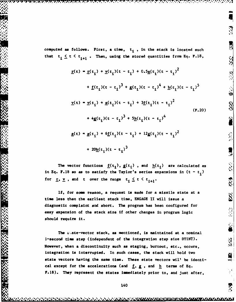
V.

Lr

computed as follows. First, a time, ti, in the stack is located such

that t l (t < t,+. Then, using the stored quantities from Eq. F.18,

- r(t) -r(t 1) + v(t )(t - ti) + 0.5a(t )(t - t )2

'-S.%°

3 45+ fti)(t - t1 ) + !(ti)(t - ti) + h(t )(t - ti) 5

v(t) - v(t1 ) + a(t )(t - t1 ) + 3f(ti)(t - ti)2 (F.20)

+ 41(tI)(t - ti)3 + 5h(tI)(t - tI)4

a(t) - a(ti) + 6f(ti)(t - ti) + 12g(t )(t - t )2

+ 20h(ti)(t - ti) 3

The vector functions f(ti), y(ti ) , and h(ti) are calculated as

in Eq. F.18 so as to satisfy the Taylor's series expansions in (t - tI )

for r, v ,and t over the range ti < t < ti+ 1.

If, for some reason, a request is made for a missile state at a

*. time less than the earliest stack time, ENGAGE II will issue a

diagnostic complaint and abort. The program has been configured for

easy expansion of the stack size if other changes in program logic

should require it.

The E,;.ate-vector stack, as mentioned, is maintained at a nominal

1-second time step (independent of the integration step size DTINT).

However, when a discontinuity such as staging, burnout, etc., occurs,

integration is interrupted. In such cases, the stack will hold two

state vectors having the same time. These state vectors will be identi-

cal except for the accelerations (and f, , and h terms of Eq.

F.18). They represent the states immediately prior to, and just after,

140

Z. 7, 2e N&

777777--

the discontinuity. The first of these two states is never used in the

interpolation scheme of Eq. F.20 since an arbitrary time will not fall

between its time and the second state's time.

OP

gS.

141

I.--•

a.i'

APPENDIX G

TARGET MOTION MODEL

The target aircraft trajectory is described by its initial condi-

tions (position and velocity), a maneuver schedule start time, and an

input schedule of maneuver segments. The initial conditions and maneu-

ver schedule start-time are generated internally by, or input to, the

program. The maneuver schedule for the target is an input array of

parameters for up to 30 segments. For each segment, these parameters

are:

0 Duration of segment

* Maneuver roll direction, *0 Maneuver magnitude (velocity vector turn rate), wv

0 Speed acceleration, av

* Bank angle1

If, during program execution, the total time duration of all seg-

ments is exhausted, the maneuver schedule will repeat from the

beginning.

Maneuver direction is defined as follows: A plane, which we'll

call the "lift plane", is perpendicular to the instantaneous velocity

vector. The unit lift vector, IL , will lie in this plane, and will be

in the direction shown in Fig. G.1, given the roll direction

The lift magnitude, aL , is computed as

aL - w vTI (G.1)

1The bank angle is not used in the present program. It was included for td

possible future use in target geometrical computations.

142

.rl.4 ..I " -i Wi#'{,a -. ?:: . ". ~~ ~ ~ ~ - 5' .' f - $ ,_ ' ' ,.., .., ... ., ' -.; I:-,S ?i,'.. ......? -A ,' 'M.7.6A , w, .-

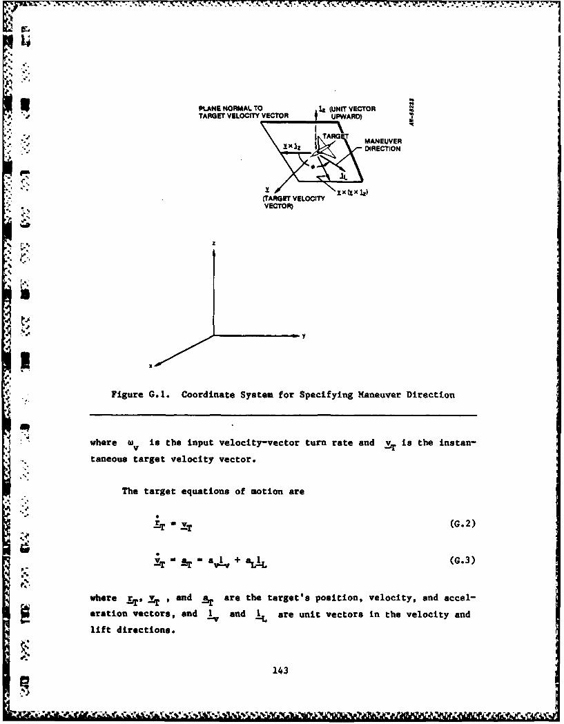
lVu

• S .

PLANE NORMAL TO 1 (UNIT VECTOR

P. TARGET VELOCITY VECTOR UPWARD) #4

. MANEUVERlx.z DIRECTION

IL"v" x(.xlz)(TARGET VELOCITYVECTOR)

z

I:..,v o,

iy

Figure G.I. Coordinate System for Specifying Maneuver Direction

where iv is the input velocity-vector turn rate and is the instan-

taneous target velocity vector.

The target equations of motion are

1T = _XT (G.2)

. - a V I + aLj (G.3)

a,.,

where ET,.xT , and a are the target's position, velocity, and accel-

eration vectors, and I and I are unit vectors in the velocity andlift directions.

143

S ......... - - - - -p~ -. -- - -

. . -7 -

During maneuver segments where w is non-zero, Eqs. G.2 and G.3

are numerically integrated using fourth-order Runge-Kutta integration

with a 1-second time-step. Integration is terminated at the end of each

maneuver segment and restarted with the next segment. For segments

which have wv - 0 (no turning), the numerical integration is bypassed

since the closed-form solutions

r(ti) " r(t) + v(t + O.5a(ti )A2

+ i - i i

V(t ) (t + a(t )A (G.4)

a(ti+i)- a(ti)

where

- - . " .A t t t + t i ( G . 5 )

can be used when the acceleration (if any) is only along the velocity

vector.

The target trajectory is maintained in a stack of up to twenty

state vectors. Whenever the model requires a target state, the current

stack is used unless the time is outside the time-span of the stack. If.-..

outside the time-span, the stack is updated by integration of the tra-

jectory (or re-initialized and re-integrated if, for some reason, the

time is earlier than any in the stack). The quantities saved for each

state vector in the stack are the time, position, velocity, acceler-

ation, and higher-order terms. These are the same as for the missile

state-vector stack described in Appendix F. The state vector for an

arbitrary time within the stack's time-span is computed by an interpola-

tion scheme which is also described in Appendix F.

144

"p"

APPENDIX H

MISSILE FLIGHT TABLE GENERATION

'* An ENGAGE II utility program, AATEST, is provided with ENGAGE II

-, . to help the user generate the input missile flight tables for a specific

scenario. Program AATEST uses the same three-degree-of-freedom flight

model as ENGAGE II, and requires the same missile input data (in the

same format) for guidance, propulsion, aerodynamics, and integration of

missile flight trajectories. (However, ENGAGE II inputs other than

missile data are not permitted by AATEST.) It interactively asks the

user for the scenario inputs desired. The missile is assumed to be

* launched at the same altitude as the target, and in direct tail pursuit.

Missile launch occurs at the center of the local coordinate system.

Both the target and the missile travel along the positive X-axis. The

program outputs the missile state vector (time, position, velocity, and

acceleration), angle-of-attack, and range (to the target) at each time

step requested for the total requested display time. Velocity and range

can be directly extracted from the output of AATEST to use as input for

the ENGAGE II AAM flight table, described below in Sec. 3.3.1. Program

use is briefly described below, and a sample output is provided as Fig.

H.l.

0 AATEST Run Description

AATEST allows the user to copy all file and terminal interactions

to the output file.

DO YOU WANT HARDCOPY OUTPUT (Y/N)

After the user types in "Y" or "N", the program reads the missile input

data, described In Secs. 3.3.4 and 3.3.5., from unit 3. Note that other

145

k-. , 2. 'eV & e 2 % .

A A

CZ.2...z

A..l w 0

a a- =a a9

:0 .2 . .. ; .65 0 . l

aa o2, N A 0 CD '

C; WmI--- . WW -O P. H-U in .. - .. . D. ..

0 00 tU N.f S ... v~ . E-4.~..

U, 4 .ou- qs. . . q C . . .4 .* 4 C - # Vr. . . .4

m0 100 0Cr .A .0 0 00 - -4.5t -W~lf - -00---00--- - -00 0irigo -.-. - --... .4 W ...O . .

E5:-r . .0; -4I (0 - -E"cz. N*... 1 6-0 'CIDU00 00 . w -. 0..Z 0 0 0s

'u-4 .C-c-~--u 5!!- 00 0 0-........0 00 0 66 00-

0 ~ U c - . .. X... . . . .0 .0 0 C~ o .I~ urdONMO C5%88~ 880N8U. N0 880

X" . . .u.. MU-N r'f I ? I I I I I I I I I I I I I I I III I I I I I I I I I I I I I I I I I I I I I I I I I I I I I I I I I I I I

----- ----- ----- ----- ---- ----- ----- ----- ----- ----

ooo~o146

.5.50.550..5.0.5..5..5..50 000.000 000 0005.50 000 0.55.55.5.*0050* *2

V0.005055.....055055505055555.*...05005..05..0..

PL

0 .

N ; *0.mto

)'. l l l l l l l l l l l l

CL.

C iY, cl 0 m ev vi 6 .> io> - N"

.41

0 000s 0 - --0-000---

0

o • . . .... .0. .. . . .

a ooooo6oooooooo

u . . .g . . . . . .

. V- *-Oo- oo0*.oo O~

W 00000000000000000+

0

0. 0. 0 .N.4 .n

I- S n.0 NU-4-ocV;-&

Z" z 0 0''-

147

* IL............................. ... . . ...... • .-..; " -,y+ , ,, . ,o ,.'..+ .. ,, - .' , 8 0..

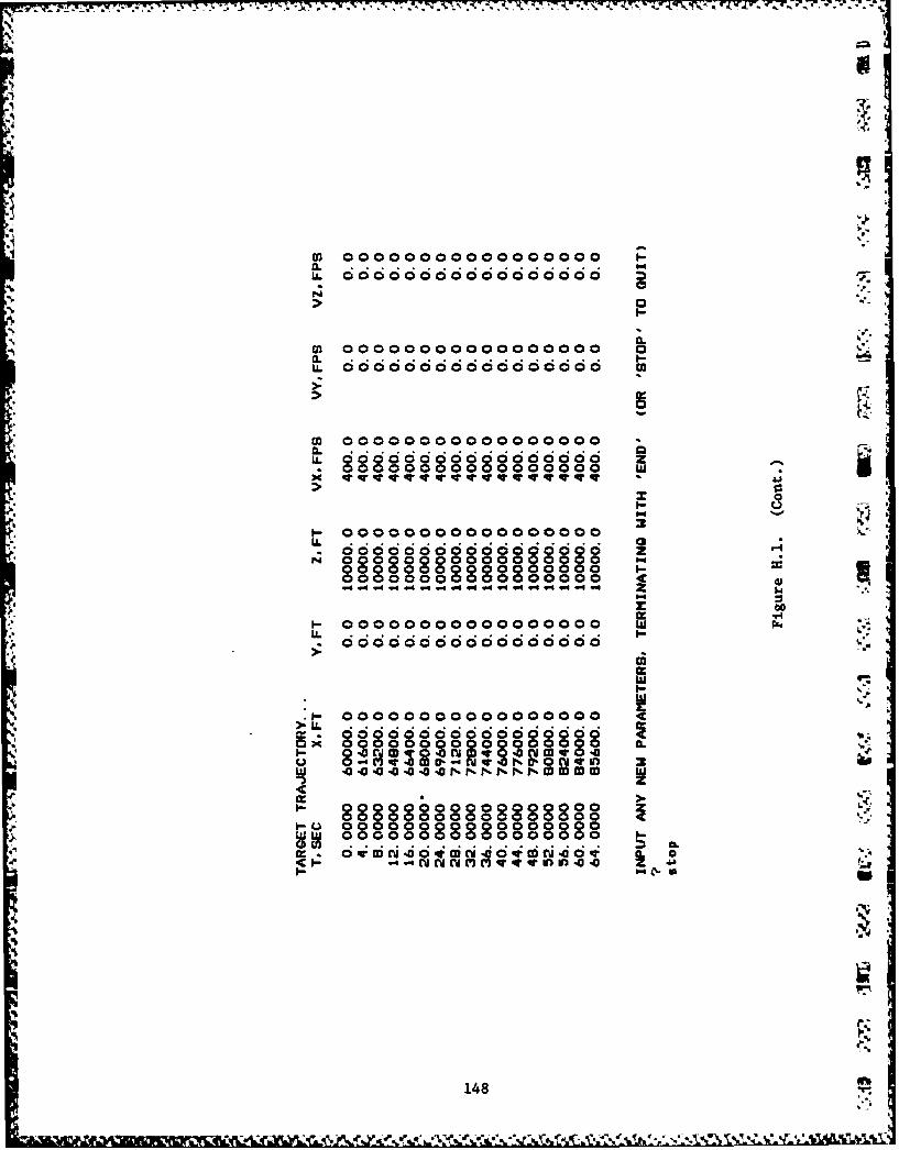
> 0

wi 00000000000000000 ~'S

.S 000 0000000

C00000000000000000 a-LL . .

C00000000000000000 z0. 000 00 00 00 0 00 00 00

L00000000000000000 Zc4. -4 4

E~ 00

t00000000000000000UL . .

100000000000000000 4c0

> 4L.4 .4 .. .4 . .. ... . . 4 .= . 000000Ox 0080001010

'5 mm o ocm 5-u qo

.4 v w~y- Nw N - rd in w

8800000000800000000 f.

* I- QQOu 000 0 5wwC 88888000800808800

m o000v -0 -w im 5.icdjo-o 4T5.-

148

ENGAGE II input data is not allowed. The user is given an opportunity

to add or change any missile data during the run.

INPUT ANY NEW PARAMETERS, TERMINATING WITH -END"

When (OR "STOP" TO QUIT)

Whnthe user has no more modifications for the missile data, he types

in "END", and then he is prompted for the mis~ile launch parameters.

INPUT ALTITUDE (FT)

The input altitude is the same for both the missile at launch and the

target.

INPUT INITIAL MISSILE SPEED, TARG. SPEED (FPS)

The user inputs two velocities, the first the velocity of the missile at

launch, which is the AI velocity, and the second the constant target

velocity.

INPUT INITIAL RANGE TO TARGET (PT)

If a complete flyout table is desired, this range should be large enough

to keep the target ahead of the missile until the total display times is

* expired.

INPUT TIME STEP, TOTAL TIME (SEC)

Total time is the total display time, usually the maximum guided flight

time of the missile. Output is generated for this period of flight

time. The time step should be chosen to provide a reasonable number of

entries for the MAM flight table, which allows a maximum number of 25

entries.

149

4 The output follows, written to the terminal and to the hard copy file,

if so requested. It includes the missile state vector (time, position

vector, velocity vector, and acceleration vector), angle-of -attack, and

range to the target at each time step for the total display time. This

is followed by the target position and velocity vectors at each of the

same time steps.

The user then may run another case.

INPUT ANY NEW PARAMETERS, TERMINATING WITH "END"

(OR "STOP" TO QUIT)

The user types in "STOP" when all cases are complete.

%%..

~*150

* .- a * S F -, ..a - * . - -

4,-

-~ 4 v~ .~ $

,,4 q

4. C

.1* 4~ 4

- lb - 4~ 1'

'ji. ~ 4: ri

4- 4- 4

1. . I?

1 4

1--* A -'C. ~. 4~ &.1& ~

'44 141t~i.

'4 '4>.4'C- 4.

- 1.

A WK

I

'4.

.~

4'

.4.

.4 :4j

4 )

4 I .25

?

p.

I K C) -

it 4r>~*.~ +t~

a,

*'1

.4

-a.- *r~ *' ' .r - S.