AD-AO92 746 NATIONAL RESEARCH COUNCIL OF CANADA OTTAWA (ONTARIO) --ETC F/G 13/6OVERLAND AND AMPHIBIOUS ACV DESIGN DATA RELATING TO PERFORMANCE--ETC(U)APR 79 H S FOWLER

UNCLASSIFIED DMEHE_245

NRC-17423 N

11111 O 116

111111.25 tH~ ff1.

MICROCOPY RESOLUTION TEST CHART

National Research Conseil national( )Council Canada de recherches; Canada

LE YE VOVERLAND AND AMPHIBIOUSACV DESIGN DATA RELATING

TO PERFORMANCE

by 0H. S. Fowler

Division of Mechanical Engineering

OTTAWA

APR IL 1979

RC NO.17423MECHANICAL ENGINEERING.-1511EWU 3REPORT

ME-245

/ OVERLAND AND AMPHIBIOUS A DESIGN DATA RELATING TO PERFORMANCE

D NNEES TECHNIQUES RELATIVES AU RENDEMENT DE /

VCA TERRESTRES ET AMPHIBIES)

] , , A,..o?

by/par ~ ~ ~ VH.S Fowler

14' lee

I

II

I E.H. Dudgeon, Head/ChefEngine Laboratory/ D.C. MacPhailLaboratoire des moteurs Director/Directeur

I(

I

SUMMARY

This handbook of data endeavours to collect and present inpractical form such design data relating to performance as are currentlypublicly available.)

The art is at present in an early stage of its development, andmany of the data given are tentative or incomplete, and are hedged aroundby ill-defined boundary conditions.

We shall attempt to keep up with the ever-shifting frontiers ofignorance by issuing amendments to this handbook as exploration proceeds.

J Finally one must remember that he who lives strictly by the rules,stagnates. Progress is attained only by knowing the rules, and then living3dangerously beyond them. _

r

RESUME

Ce manuel de donn~es tente de faire la compilation et de presentersous une forme pratique des donn~es techniques relatives au rendement devihicules i coussin d'air (VCA), dans la mesure o4 de telles donn~es sontcouramment disponibles pour le public.

Pr~sentement, ce domaine n'en est encoure qu'aux toutes pre-mieres 6tapes de son d6veloppement, et nombreuses sont les donnr6es qui nesont proposes qu'i titre provisoire ou qui sont incompltes et dont lesconditions limites sont plus ou moins bien d6finies.

Nous tenterons de rester i jour malgr6 le recul sans cesse constantdes frontiires de l'inconnu, en publiant des modificatifs au fur et i mesuredes recherches.

Enfin, il y aurait lieu de ne pas oublier que la stagnation est le fruit

de l'observance stricte des r~gles. Le progris n'est possible qu'en tenant

compte des r~gles puis en se risquant ensuite au deli des limites prescrites parces mimes rigles.

00

0 -

r: C)

(ii) °

CONTENTS

Page

SUMMARY ................................................................................................................... (iii)

ILLUSTRATIONS ....................................................................................................... (v)

1.0 AIRSPEED ................................................................................................................... 1

2.0 CENTRIFUGAL FAN LAWS ...................................................................................... 7

3.0 LIFT FORCE AND LIFT AIRFLOW ........................................................................... 9

4.0 THRUST ...................................................................................................................... 12

4.1 Measurement ................................................................................................... 124.2 Calculation of Aerodynamic Thrust ................................................................. 12

5.0 DRAG .......................................................................................................................... 15

5.1 Drag Overwater at 'High' Speed ....................................................................... 15

5.1.1 (A) External Aerodynamic Drag ("Form Drag") ................................ 155.1.2 (B) Lift Air Momentum Drag ............................................................. 155.1.3 (C) Wavemaking Drag .......................................................................... 155.1.4 (D) Spray Momentum Drag ................................................................. 175.1.5 (E) Skirt Friction Drag ........................................................................ 17

5.2 Drag Overwater at 'Low' Speed ........................................................................ 185.3 Drag of Overland ACVs .................................................................................... 24

6.0 ROLL AND PITCH ...................................................................................................... 28

7.0 HEAVE STABILITY .................................................................................................... 30

8.0 A SIMPLE LOW-SPEED ANEMOMETER ..................................................................... 31

9.0 RATE OF FALL OF SPHERICAL PARTICLES .......................................................... 32

10.0 EFFECT OF ALTITUDE AND TEMPERATURE ON PERFORMANCE ..................... 34

10.1 Standard Day, Sea Level ................................................................................... 3410.2 Recalculation for Arctic Sea Level Condition ................................................... 3510.3 Recalculation for Hot-Day at 1067 m Altitude (= 3500 ft. = Calgary) .............. 35

11.0 TERMINOLOGY AND NOTATION ............................................................................ 36

11.1 Terminology Peculiar to ACVs, Primarily Overland or Amphibious ................ 3611.2 Notation ........................................................................................................... 44

12.0 REFERENCES ............................................................................................................. 46

(iv)

CONTENTS (Cont'd)

Page

13.0 SI UNITS AND IMPERIAL EQUIVALENTS ............................................................... 47

14.0 ACKNOWLEDGEMENT .............................................................................................. 49

ILLUSTRATIONS

J Figure Page

1 Suction and Blower Systems ..................................................................................... 1

2 Static and Total Pressure Probes ............................................................................... 3

3 Airspeed vs. Dynamic Pressure (Low Speed) ............................................................. 4

4 High Pressure Cushion-Air Temperature and Escape Velocity ................................... 5

5 Air Temperature, Pressure and Density at Various Altitudes ...................... 6

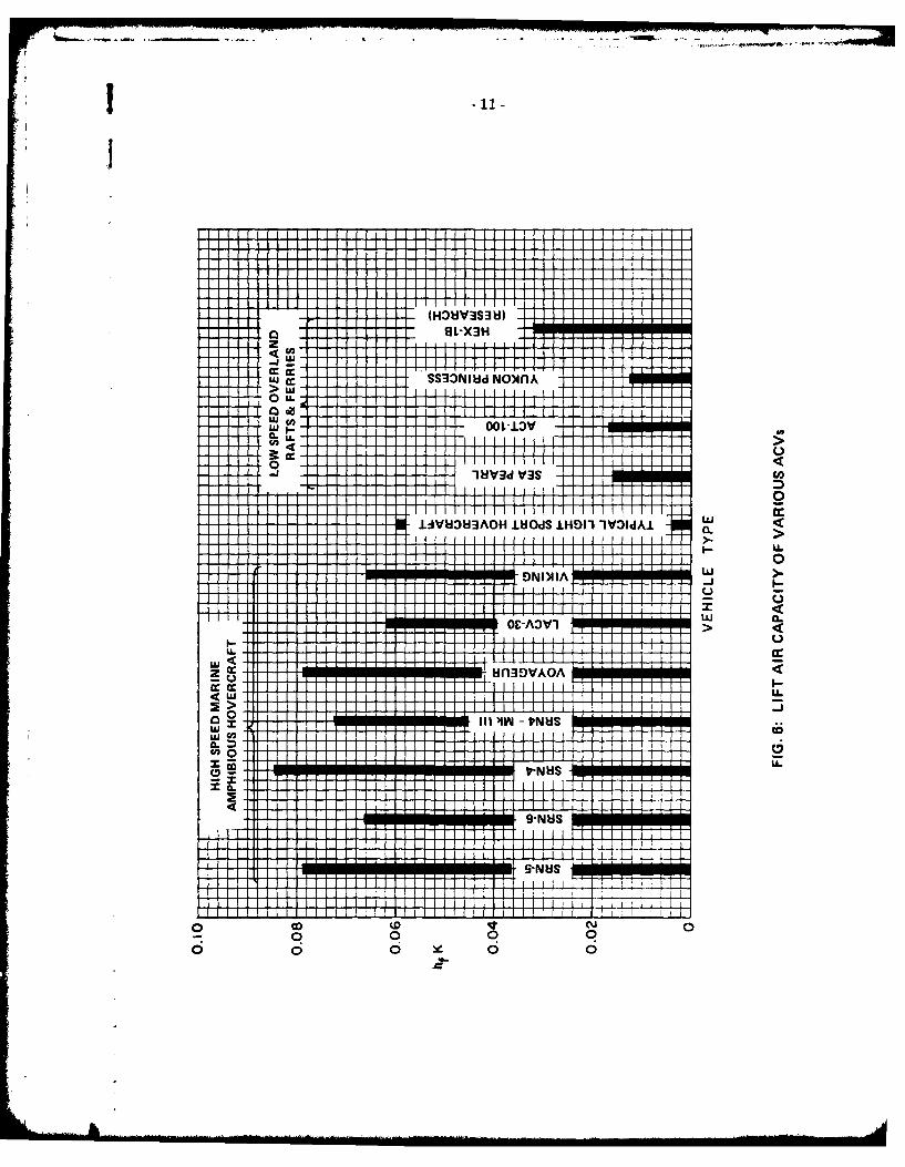
6 Lift Air Capacity of Various ACVs ........................................................................... 11

7 Fan Performance (Thrust/Power/Area) ..................................................................... 14

8 Typical Aerodynamic Drag Coefficients (at Zero Yaw) ............................................. 16

9 O verwater D rag ......................................................................................................... 18

10 Thrust Requirement for Amphibious Hovercraft ...................................................... 19

11 Low-Speed Overwater Drag of HEX-5 ....................................................................... 21

12 Derived Drag Coefficient for HEX-5 ......................................................................... 22

13 Measured Wave Drag of Yawed ACV ........................................................................ 23

14 Variation of Wave Drag With Yaw and Froude No .................................................... 23

15 Efflux Gap Height vs. Skirt Drag Coefficient ............................................................ 25

16 Skirt Drag vs. Speed at Various Efflux Gap Height ................................................... 26

17 Change of Drag With Repeated Passes Through Deep Grass ..................................... 27

18 Roll Stiffness of Typical Skirts ................................................................................. 29

19 V.K.I. Low-Speed Anemometer ................................................................................ 31

" 20 Rate of Fall of Small Spherical Particles in Air .............................. 33

(v)

ILLUSTRATIONS (Cont'd)

Figure Page

21 ACV Co-ordinate System .......................................................................................... 40

22 Features of Segmented (HDL) Skirt System ............................................................. 41

23 Features of Flexible Trunk and Finger (BHC) Skir System ..................................... 42

24 Features of Basic M ulticell (Bertin) Skirt System ..................................................... 43

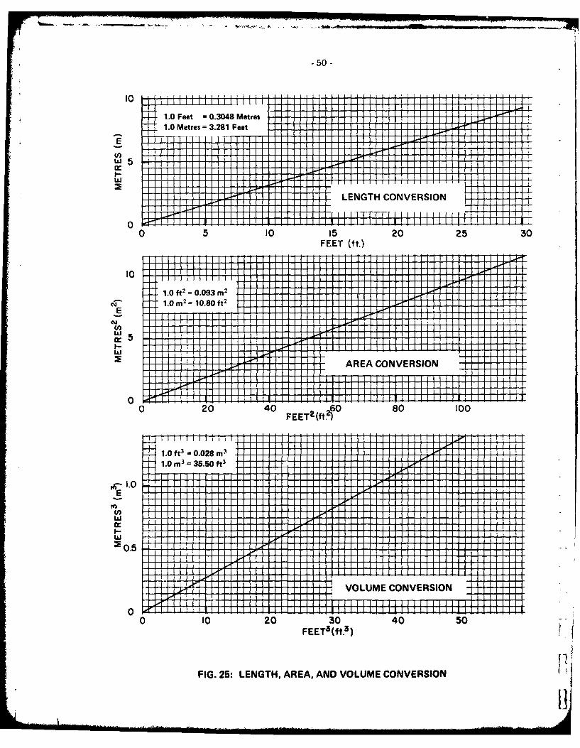
25 Length, Area, and Volume Conversion ..................................................................... 50

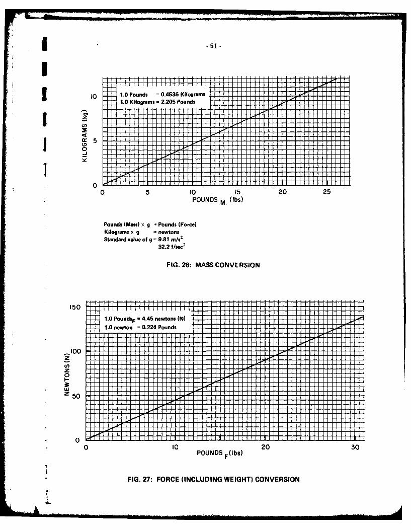
26 M ass Conversion ....................................................................................................... 51

27 Force (Including W eight) Conversion ........................................................................ 51

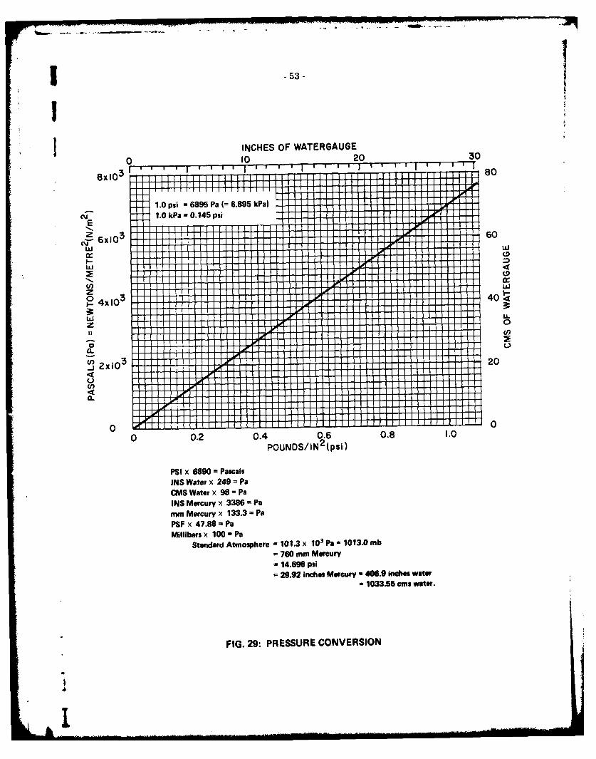
28 Temperature Conversion ........................................................................................... 52 1.29 Pressure Conversion .................................................................................................. 53 -

30 Air Density Values and Conversion .......................................................................... 54

31 Speed Conversion ..................................................................................................... 55- L.

32 Power Conversion ..................................................................................................... 56

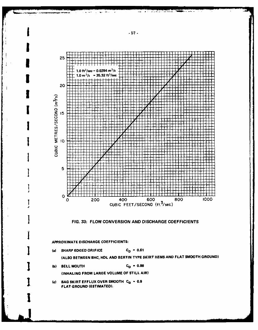
33 Flow Conversion and Discharge Coefficients ............................................................ 57

(-!.

V

(vi)

I OVERLAND AND AMPHIBIOUS ACV DESIGN DATA RELATING TO PERFORMANCE

1.0 AIRSPEED

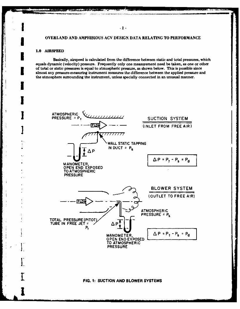
Basically, airspeed is calculated from the difference between static and total pressures, whichequals dynamic (velocity) pressure. Frequently only one measurement need be taken, as one or other

* of total or static pressures is equal to atmospheric pressure, as shown below. This is possible sincealmost any pressure-measuring instrument measures the difference between the applied pressure andthe atmosphere surrounding the instrument, unless specially connected in an unusual manner.i

II ATM OSPHER IC

PRESSURE Pt< SUCTION SYSTEM

-- D (INLET FROM FREE AIR)

WALL STATIC TAPPING- -IN DUCT Ps

APAP et - Ps =PdMANOMETER,OPEN END EXPOSEDTO ATMOSPHERICPRESSURE

_BLOWER SYSTEM

(OUTLET TO FREE AIR)

ATMOSPHERICPRESSURE Ps

TOTAL PRESSURE (PITOT)TUBE IN FREE JET a P, _ __Pt

MANOMETER, A P P "S PdOPEN END EXPOSEDTO ATMOSPHERICPRESSURE

F? FIG. 1: SUCTION AND BLOWER SYSTEMS

I

-2-

where P, = Total Pressure (Pa)

P, = Static Pressure (Pa)

Pd = Dynamic Pressure (Pa)

From Bernouilli's equation, we have the fundamental relationship1 L

Pd pV 2 (2)2i

where p = Air Density (Kg/m 3 )

V = Air Velocity (m/s)

Pd = Dynamic Pressure (Pa)

The above equation may be rearranged to the form:

Pd X tKV - 0.756 (3)

Air Press. (kilopascals)

This calculation may be used up to about 150 m/s. Above this the flow must be assumed to be com-pressible, and calculated by iteration from the formula:

7

Pt 7-1,'Y-1- = (1 +- M 2 (4)

4)2 n

where y = RATIO OF SPECIFIC HEATS (= 1.3984 for air) "

Mn = Mach No.

(where Mach Number is defined as Velocity relative to gas (at local static temperature).Velocity of sound in gas

VAt standard sea level atmospheric conditions, this becomes - (V in m/s).

The function Pt/Ps is usually displayed on compressible flow curves or tables for easy reference.

m

.J -3-

2 DUCTWA LL

lii~...TUBE TOMANOMETER

STATIC PRESSURE WALL TAPPING

* WALL SURFACE MUST BE DEAD SMOOTH AROUNDTRULY FLUSH HOLE, WHOSE AXIS IS NORMAL TOSURFACE. NO RAGS, BURRS, OR COUNTERSINK.

HOLE DIAMETER - I mm. TO 4 mm.

I AT LEAST 3D _I

[ " INSI!DE OF PROBE'

, CHAMFERED THUSTHIS FACE SHARPEDGED & SQUARE

TO AXIS TO

TOTAL PRESSURE (PITOT) PROBE MANOMETER

THE INSIDE CHAMFERED NOSE MAKES THIS PROBEINSENSITIVE TO AIRFLOW DIRECTION UP TO±300

D OUTSIDE DIAMETER = 2 mm. TO 7 mm.

FIG. 2: STATIC AND TOTAL PRESSURE PROBES

IJ

-4.-1

3000 "i. 71 F; u14~~...30200 20

-4:-

*-. LLUL

1000 .. . .. 1_ E_ _ I

-K ---~~- .. .... ...- - - -

-r - ia

~ ' I

I *I

200 i~IIV 1. 275 [P d (Pd in Po)AT STANDARD DENSITY (P 1.23 Ikg/m)

0 20 40 60 80 100AIR SPEED V (m/s)

2 jj-oo

- 0i

LUU

00C-j

w CL

UJI

4LL

LU

0c

I I -

LU C.

0 C

CL Lt0 0 0CID 0 IV(Dd) unSS8d NICn

-6-

rn 100,000

OD 90,000

(D E80, 000 -

a. V)

ww

0 U

o CD o 50,000I I~ +00 200 3000 I4005 0

ALITD\(n

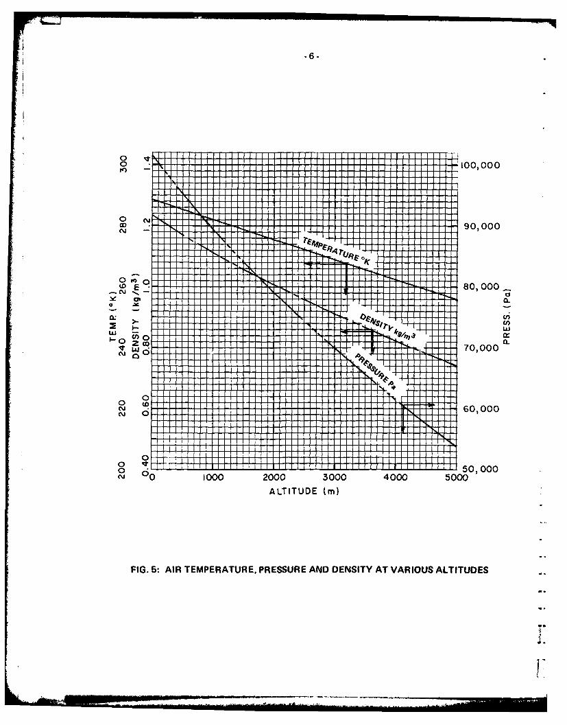
FIG.~~~~~ 5: Ti EPRTRPESR N EST TVROSATTDS-

I I I I N

-7-

a 2.0 CENTRIFUGAL FAN LAWS

Pressure Rise

APt = p(U 2 0)r (5)

[for radial vane blowers]

where APt = Total Pressure Rise (Pa)

p = Air Density (kg/m 3 )

U = Tip Speed of Impeller (m/s)

a = Slip Factor (usually taken as 0.9)

17C = Efficiency (between 0.65 and 0.75)

Note,

RPMU - X 7r X Diam. (Diam. of rotor in metres). (6)60

Or for impellers with swept-back vanes, whose exit direction is at 00 to the tangent to the impellerperiphery:

APt = p(Tip Speed (Tip Speed - Vrcos ° )o0 )a) (7)

where Vr = Calculated radial velocity at impeller exit - (m/s).

This formula gives approximate results only, since 00 and V, are not easily estimated.

Fan Power

The power required to drive the fan (not accounting for drive, transmission, or bearinglosses) is:

Volume Flow X Pressure Rise 1Power = X -in kilowatts (8)1000 77c

If duct losses are to be included in the calculation, a term 7d is used (for duct efficiency), which mayvary from 0.9 for good fan volute delivering low-speed air directly into the cushion to 0.25 for a com-plex duct system.

* Then,

Vol. Flow X APt 1 1

Power = X - X - = power(kw) (9)1000 77c d

The so-called "Fan Laws" which permit predictions of the performance of the same fan atvarious conditions, or of geometrically similar fans, are as follows. These statements should be takenas approximate guides, and demand some experience for successful application.

... .. . . .. .... ............. ... ...Il ..... ..] ......[..... ..

-8.

(a) For the same Impeller and Volute at a Range of Conditions.

Qv1 RPM,-- = RPM2 (1 and 2 are two running conditions) (10)

t2 /RPM\

/RPM, 2 (11)= t2 RPM2Y

HPI 1RPM,\ 3

HP2 \ RPMV/(2

(b) For Geometrically similar Impellers and Volutes (NB Impeller width varies with tip diameter)

D-2- (1 and 2 are similar impellers) (13)At2 \D 2/

Qv_ (Dl\ 3

Q-v2 D (14)

HP1 D\

HP 2 D2 (15)

where Qv = Volume Flow - (m3 /s)

APt = Rise of Total Pressure - (Pa)

HP = Power - (kw)

D = Tip Diameter - (m)

RPM = Revolutions/minute

Centrifugal Force (on a body of weight W(N) moving around a centre at radius R(m) at N (Revs/sec))

CENT. FORCE (newtons) = W R N2 X 4.024 (16)

W V2

or C.F. (N) = W (17)Rg

where V - Tangential speed (m/s)

g - Accel. due to gravity (9.81 m/s 2 )

1 -9-

i 3.0 LIFT FORCE AND LIFT AIRFLOW

The Lift Force being exerted on an ACV at any moment must equal its total weight at thattime (dynamic effects excepted). Clearly also the lift force must equal the product of cushion pressuretimes footprint area. However, although cushion pressure can be measured with good accuracy, thefootprint area of a flexible skirt is very difficult indeed to measure, so (pressure X area) is not anacceptable test method. The only useful method of measuring lift is to weigh the vehicle (including

*fuel, freight, crew, etc. to give total weight).

For a given vehicle total weight, Lift Airflow can vary widely according to terrain, skirt, and* lift blower characteristics, and to the operating point which the driver chooses on the lift airflow/

1 j hoverheight/drag curve. This subject is discussed in detail in References 1, 2, and 3 which should beconsulted.

It should be noted that this discussion relates only to the airflow blown into the cushion andused for lift. This includes leakage between segments, seals, etc., but does not include air "stolen" forengine flow, cooling, and other non-lift uses.

I Following the argument of Reference 2, lift airflow is expressed by equation:

L hfK 2 w

V 0 V (18)VE

where Lift airflow = Q (m3 /s)

Skirt perimeter = L (M)

Efflux gap height = h or hf (M)

Discharge coefficient = CD

Air density of day = p (kg/m 3 )

Total vehicle weight = w (N)

Footprint area = Sc (m2 )

Cushion pressure = PC Pa (gauge)

The discharge coefficient CD is that for flow between a skirt hem and flat ground, (0.61according to standard text books such as Lamb's Hydraulics, sharp-edged orifice data, and NRC tests),hf is the efflux gap height over flat nonporous ground at low speed, while a factor K (or possibly agroup K, K2 etc.) represents the increase of h required due to terrain porosity, uneveness, highspeedoperation, wave pumping, etc. This factor will be discussed later; at present it will simply be includedin the equation and the results presented in Figure 6, given in terms of the factored efflux gap heighthfK.

In the above equation it is clear that the various terms have real physical significance.

The term is related to vehicle planform, or aspect ratio. The term 1 describes the

atmospheric conditions, and is of surprising importance in designing and testing a vehicle for use in the

I

-10-

arctic, or on a hot high-altitude plateau. considers both the cushion pressure and the total weight

hvKof the vehicle, and might be called a "loading" term, while the term - defines the efflux gap in a

non-dimensional manner. VO

The convenience of the above equation to a designer is therefore apparent, since it enableshim to see at a glance the effect of juggling the several variables open to him in meeting a particularrequirement, and at the same time ensures that by using a value of hfK appropriate to the terrain andoperational mode specified he will produce a vehicle with adequate hovering performance by currentlyaccepted standards.

Returning now to reality, it is well known (and clearly demonstrated Fig. 6) that variousclasses of air cushion vehicles operate at considerably different values of lift airflow, expressed here asvalues of hfK.

In the high speed marine "hovercraft", the very high value of hfK is designed partly to reduce

skirt drag and wear by minimizing (within practical limits) skirt/wave contact, and partly to offset theI

The low speed over-water/mud-flat A.C. ferry barge operates at an extremely low hfK sinceit has only small frictional and sealing demands to contend with.

Experiments with the CASPAR vehicles and other scattered clues lead us to believe thatoperation over notably rough ground or porous vegetation at low speed, or high speed operation overflat ground, will require larger values of hfK but still not up into the marine "hovercraft" range. p

I

I

Ii

*j H 1 114-

a Jb

w~~~ <-

0

C-)

U. cU

LE un39VAOA

CA 0 0 1 1110 0o IVN0 H

9--U

.12 -

4.0 THRUST

The thrust exerted on an ACV by its propulsion system can be generated in a number ofways - by aerodynamic means (propellers, fans, or other airjets) or by terrain contacting systems suchas wheels, tracks or underwater screws.

4.1 Measurement

It is simple to measure the static thrust (i.e. the thrust generated while the vehicle is station-ary and pulling at measuring device) but the measurement of thrust while moving is more difficult. Theonly reasonably direct method of measuring moving thrust is to make a series of runs on standardterrain at a series of speeds and engine RPM, and then repeat these runs while towing the ACV, with itsthrust system inoperative, and measuring the tow force required at each speed. Even then, a number ofsources of error (mainly concerned with the drag of the unpowered propulsion unit) make the resultsless than reliable.

Static thrust may be measured directly by the tension in a restraining cable while the ACVhovers over smooth ground forming its own frictionless bearing. As a matter of detail, the anchor (atruck or other heavy vehicle) should be at least two vehicle lengths behind the ACV, to ensure thatthere is no aerodynamic interference, and the cable should be horizontal, with the scale or strain gaugebetween cable and ACV, (not between anchor and cable) to eliminate errors due to cable weight. It isalso necessary to run the experiment twice, facing in opposite directions with the ACV on the samespot so that the average value of thrust will eliminate the effect of any slight wind or slope in theground. If this is impossible, then the slope of the ground must be checked with an accurate level atthe actual place occupied by the ACV. Even a slope of 1 in 100, which is hardly perceptible to theeye, will introduce an error of 1% of the weight of the vehicle, which is a 10% error of the thrustcommonly installed in ACVs.

Static thrust may also be measured, provided the ACV has a lift system completely separatefrom its thrust system, by hovering the vehicle on a slope (which pretensions the cable) and then gen-erating thrust, which will equal the difference of gauge reading between slope only and slope plus .

thrust-on cases.

It is also necessary in all cases to see that the vehicle is trimmed level, as an unequal hovergapor tilted hull can generate thrust from the cushion which will upset the results.

Theoretically, aerodynamic thrust can be measured by measuring the velocity and quantityof air leaving the thrust duct or propeller disc. However, it is so difficult to measure this non-uniformjet and integrate these quantities successfully that this method should not be attemped for thrust !measurement.

4.2 Calculation of Aerodynamic Thrust

This subject has been discussed in detail in Reference 4 which should be consulted.

Briefly, Thrust = Change of momentum of air passing through thruster.

= Mass flow/sec X increase of velocity.

Assuming zero inlet velocity to the thruster

' Thrust - mass flow/sec X exit velocity [Static thrust]

where Thrust - (newtons) = T

Mass flow - (kg/s) = Qm

Exit Vel. - (m/s) = V

* - 13 -

I Converting to Volume Flow,

T = (V X p X A) X V X CD.

T = V2 pA CD of the exit jet. (19)

I where p = Air density (kg/m 3 )

A = Nozzle area (M2 )

CD = Discharge coefficient (varies from 0.95 from a good nozzle or thrust duct to 0.6 for asharp edged flat plate and 0.5 for flow through an unducted propeller disc of area A).

IThis makes it clear that any aerodynamic thrust calculations must account for air density, with itsconsiderable variation from summer to winter, and from sea level operation to work on a high plateau.One should note that even in the Canadian Prairies, at 1000 metres altitude, the air density is down to1.10 kg/m 3 instead of sea level value of 1.23 kg/m 3 , - a change of 10% for the worse!

For a standard aircraft-type propeller or fan the thrust is usually expressed as a Thrust Co-efficient (T,), which accounts for atmospheric conditions:

Thrust = T€ X p X (Revs/sec)2 X (Fan tip diam.) 4 (20)

A very useful set of relationships for ducted fans or open propellers is shown in Figure 7. Itis derived directly from momentum increase through the fan, for the lowspeed or static case. Thederivation is discussed at length in Reference 4.

The relevant quantities are plotted in the following form.

(a) THRUST/POWER - (N/kw) - (Conversion N/kw X 0.168 = lbs/HP)

(b) POWER /FAN DISC AREA - (kw/m 2 ) - (kw/m 2 X 0.125 = HP/ft2)

(c) THRUST/FAN DISC AREA - (N/m 2) - (N/m s X 0.0205 = lbs/ft2)

F.M. is the "Figure of merit", and represents a fan efficiency. An FM = 1.0 implies that thethrust developed is the theoretical maximum under the circumstances.

A Figure of merit of 0.8 is good for a ducted fan with an aerodynamically clean intake,while 0.6 is not surprising in a practical installation. On the same calculation basis, a centrifugal fanblowing air out through a thrust nozzle, as installed on a number of smaller ACVs, is likely to have a

- F.M. of around 0.3 largely owing to bend losses in the blower and volute, and to the small high-speednozzles usually employed in the absence of a large and clumsy diffuser. In these cases the "fan discarea" is of course the propulsion nozzle area.

It is frequently difficult to assess the thrust system, since valid engine power figures are verydifficult to obtain. Those quoted are often attainable only for one or two minute bursts, while thereliable continuous power is far lower.I

I1I

.14 -

r0

LU

LLLU

77)

I AU

0

U-

o' /N C\Md/SflLL

-15-

5.0 DRAG

5.1 The drag of a highspeed over water ACV is fairly well understood, and is made up of fivecomponents, as itemized below, to which must be added the underwater drag of any submerged parts(keels, skegs, rudders, propellers, etc.) if present, as in non-amphibious craft. This latter is calculatedaccording to standard marine practice. The analysis shown below follows the treatment given byTrillo (Ref. 5).

Total Drag = External Aerodynamic Drag (A)

+ Lift Air Momentum Drag (B)

+ Wavemaking Drag (C)

+ Spray Momentum Drag (D)

+ Skirt Friction Drag (in water contact) (E) (21)

5.1.1 (A) External Aerodynamic Drag ("Form Drag")

1DA p V2 A CDA in newtons (22)

2

where p = Air Density - (kg/m 3 )

V = Craft Speed relative to the air - (m/s)

A = Frontal Area at max. section - (m 2 )

CDA = Drag Coefficient (Varies from 0.3 to 0.6, with 0.3 to 0.5 as most likely values. Thevalue for an ACV could easily rise to 0.8 at 900 yaw. (See examples on page 16 -Fig. 8) (See Ref. 6).

5.1.2 (B) Lift Air Momentum Drag(drag of lift air inhaled and accelerated to craft speed)

DM = Qm V in newtons (23)

where Qm = Mass flow of lift air - (kg/s)

V = Craft speed relative to air - (m/s).

5.1.3 (C) Wavemaking Drag

*At low speed the ACV acts as a displacement boat, and raises a large wave system. At acritical speed ("Hump speed", so-called from the hump in the drag curve) the ACV rises above thewater, and planes. The wave system almost vanishes and wave drag is sharply reduced. In order topass the critical speed and perform satisfactorily in the planing mode, the craft needs a thrust equal toroughly 1.5 or 2 times the hump wavemaking drag (as a rough approximation).

Hump Speed = k,/Q (24)

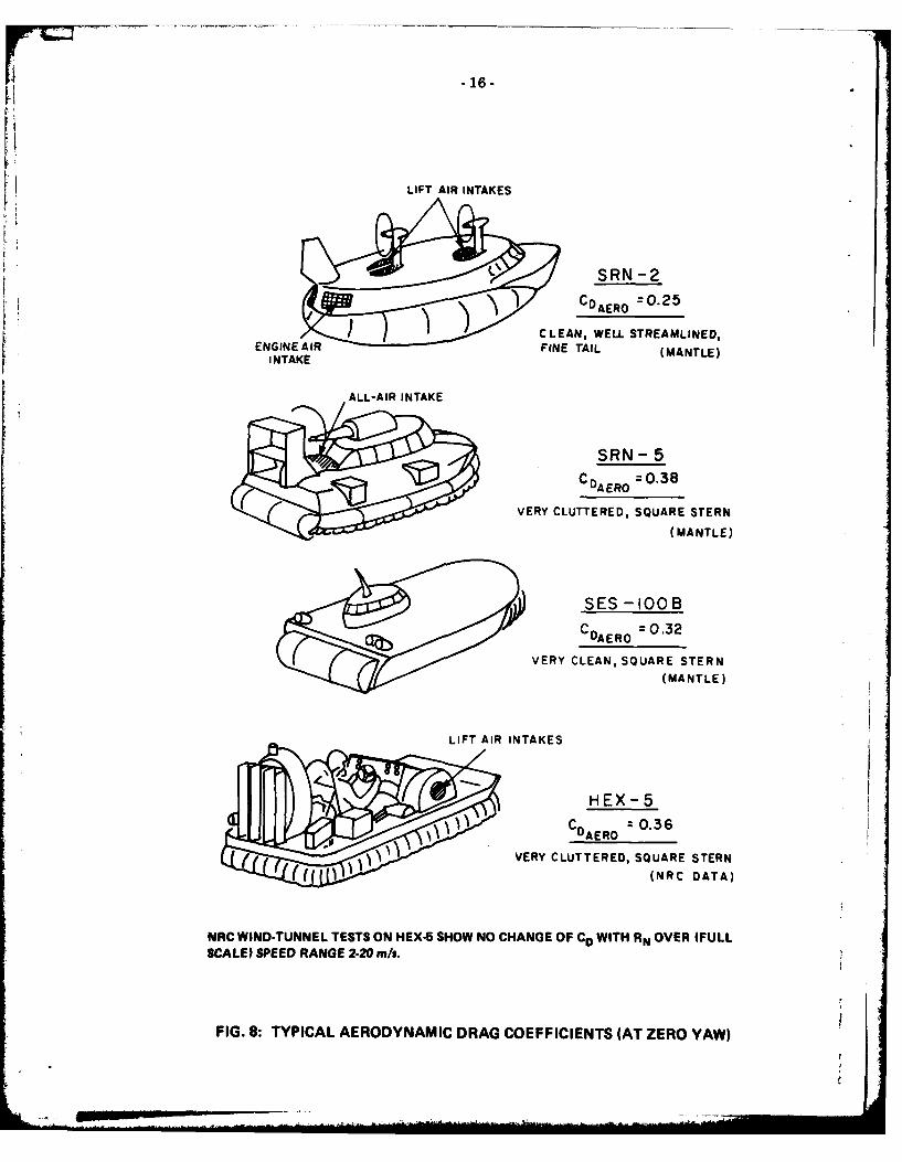
-16-

LIFT AIR INTAKES

SRN -2CDAERO 20.25

CLEAN, WELL STREAMLINED,ENGINE AIR FINE TAIL (MANTLE)

INTAKE

ALL-AIR INTAKE

SRN - 5

C 0DAERO =.38

VERY CLUTTERED, SQUARE STERN

(MANTLE)

SES -100 BCDAERO = 0.32

VERY CLEAN, SQUARE STERN

(MANTLE)

LIFT AIR INTAKES

HEX-5

c = 0.36" CDAERO

VERY CLUTTERED, SQUARE STERN(NRC DATA)

NRC WIND-TUNNEL TESTS ON HEX-5 SHOW NO CHANGE OF CD WITH RN OVER (FULLSCALE) SPEED RANGE 2.20 m/s.

FIG. 8: TYPICAL AERODYNAMIC DRAG COEFFICIENTS (AT ZERO YAW)

-17-

* where Speed = Craft speed relative to water - (m/s)

2 = Cushion length - (m)* k = a constant between 1.4 and 1.8 (theoretically 1.76)

Wavemaking drag at hump speed is known as Hump Drag (DH) and

0.03 X M2

DH X Factor (in newtons) (25)Sc X

where M = Craft Mass - (kg)

j Sc = Cushion footprint area - (M2 )

£ = Cushion footprint length - (m)

I and the Factor depends on the water. Approximate values given by R.G. Wade are:

Smooth deep water = 1

Rough deep water = 2

1 Shallow water = 3

These factors apply to a cushion planform aspect ratio of 2:1.

I5.1.4 (D) Spray Momentum Drag

S This accounts for the acceleration up to craft speed of spray taken on board or thrown up

beneath the skirt, and includes a very empirical constant.

jIt obviously depends also on the sea state

1 6.51,000,000 X SC X PC X X V in newtons (26)

where Sc = Cushion area - (M2 )

PC= Cushion pressure - (Pa)

2 = Cushion footprint length - (m)

h f hovergap - (m)

V = Craft speed relative to water - (m/s)

I 5.1.5 (E) Skirt Friction Drag (Wave contact)

1 DSF = 4.2 X Sc X a X V2 in newtons (27)

I

- 18 -

where Sc = Cushion area - (m2 )

a = Wave height - (m)

V = Craft speed relative to water - (m/s)

This term can be very large.

These drags combine to form the total drag of an overwater ACV. Their relative proportionsin a typical case have been shown diagrammatically in various sources (Ref. 7 etc.) by the figure (Fig. 9).

DRAG IN ROUGH

_ WATER /

/ /

I \ 4

CALM WATERDRAG

Wu0.

FIG. 9: OVERWATER DRAG(After Elsely & Devereux)

The full lines represent a calm-water situation, and a dotted line suggests the additional dragin a rough sea (wave height approximately equal to skirt height).

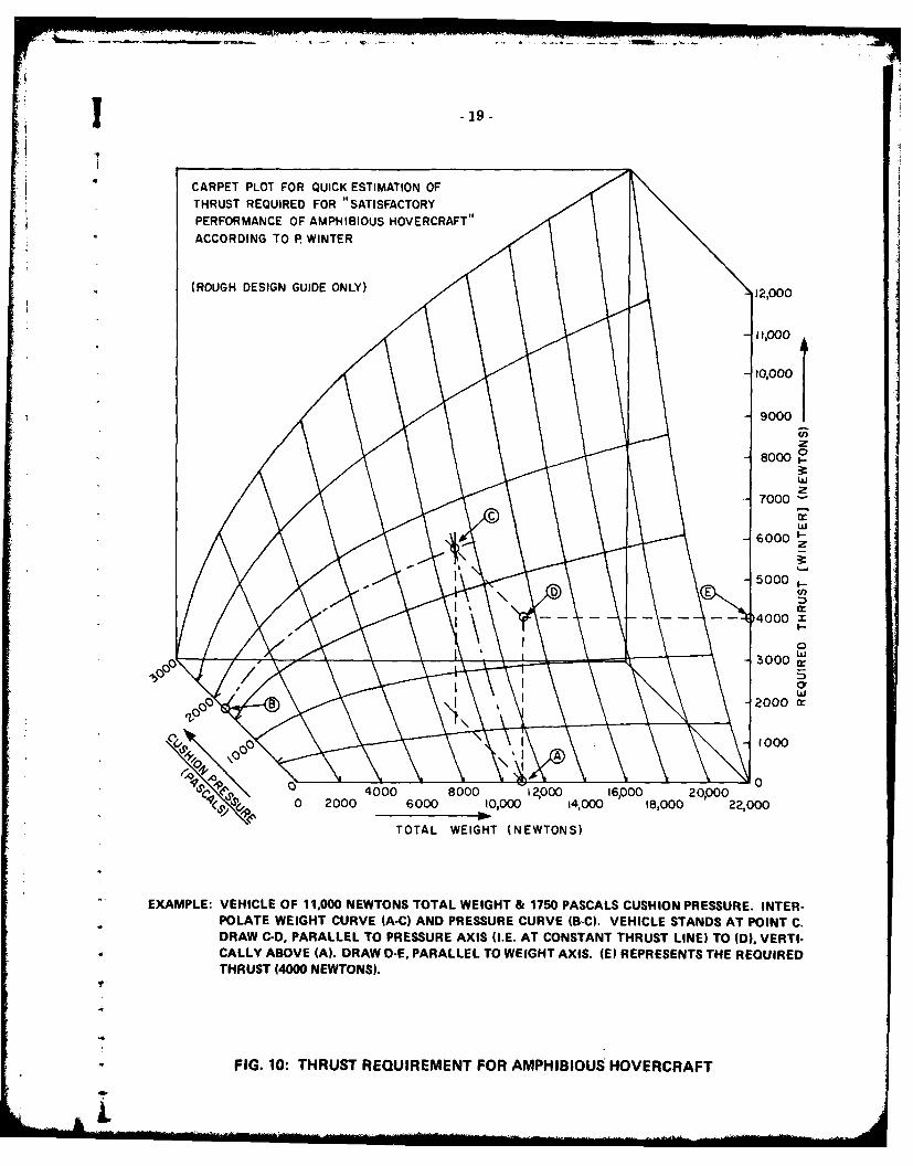
While on this subject, one may quote Winter, who remarks in a report that "for satisfactoryperformance (of a light ACV, of say up to 25,000 N total weight) the installed thrust should be about2.5 times the calm-water hump wavemaking drag". For very approximate estimating purposes, Figure 10sets out this thrust requirement.

5.2 Drag Overwater at 'Low' Speed

It appears that at present there is a great lack of reliable published data for predicting over-water drag of ACVs at low speed. Until better data and methods are available, the following approachis suggested.

-.19 -

CARPET PLOT FOR QUICK ESTIMATION OFTHRUST REQUIRED FOR "SATISFACTORYPERFORMANCE OF AMPHIBIOUS HOVERCRAFT"

ACCORDING TO P WINTER

(ROUGH DESIGN GUIDE ONLY) .2,0

11000

B900

0

- 7000

CW

6000

5- 00000

)4000

~3000

B@ 2000, 2

-"0 , 4000 B000 1, 000 16,000 20,000 0°19 0 1oo o ,~o4,000 22OO ,000

TOTAL WEIGHT (NEWTONS)

EXAMPLE: VEHICLE OF 11,000 NEWTONS TOTAL WEIGHT & 1750 PASCALS CUSHION PRESSURE. INTER-POLATE WEIGHT CURVE (A-C) AND PRESSURE CURVE (B-C). VEHICLE STANDS AT POINT C.DRAW C-D, PARALLEL TO PRESSURE AXIS (I.E. AT CONSTANT THRUST LINE) TO (D). VERTI-CALLY ABOVE (A). DRAW D-E, PARALLEL TO WEIGHT AXIS. (E) REPRESENTS THE REQUIREDTHRUST (4000 NEWTONS).

FIG. 10: THRUST REQUIREMENT FOR AMPHIBIOUS HOVERCRAFT.i

. .............. .. . .... . ..o ., -4--- : : := .. . S

-':

_ -. ' :- -r

-20-

At low speeds the following simplifying assumptions may be made:

(a) In the range up to 0.5 X hump speed, Aerodynamic and Momentum drags are negligible, andcan be accounted for under total drag without serious error.

(b) In this range wavemaking is observed to be small, and wave drag can also be neglected.

(c) To define this range, the standard theoretical value that Hump Speed = 1.76Vcushion length(speed in m/s, length in m) may be used.

In this speed range, the total drag would appear to be substantially the form-drag of a bluffbody towed under water, and defined by the area of skirt below water across the bow of the craft. Thisis clearly equal to the product of (cushion beam X cushion pressure in height of water gauge units).

Form drag is calculated from the standard formula:

D = 1 p V 2 A CD (28)

where D = Drag (newtons)

p = Density (of water = 1000 kg/m 3 )

V = Craft Speed relative to water (m/s)

A = Opposed area (of skirt) = b X P, (m2)

CD = Drag Coefficient (see following argument).

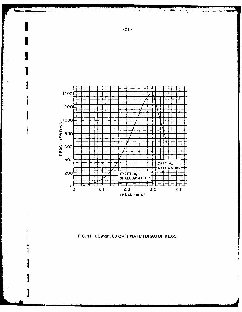
The drag coefficient CD must be found experimentally, and the attached curve (Fig. 11) gives anopportunity to estimate it for vehicle HEX-5.

Using the method stated above, a curve of CD vs. speed derived from the speed vs. drag curveis shown in Figure 12.

The procedure for calculating the drag of any similar vehicle is therefore as follows:

1. Hump speed is calculated, as VH 1.760 -

2. The method may be used up to V = V H 1 /2.

3. Vehicle speeds in m/s are calculated, corresponding to a series of percentages of VH up toVH/2.

4. From Figure 12 the CD values at each of these percentages of VH are read off.

5. Using the CD values appropriate to each speed, the equation D = CD A P V 2 has the seriesof speeds substituted in it, and values of the drag D may be read off. 2

Drag measurements on HEX-5 while carrying a heavy load of ballast have fallen on a curvepredicted from this data, and future experiments on HEX-IB, (geometrically similar but approximatelytwice the size) will be made at the earliest opportunity to further confirm the validity of this appxnach.

-ram-

I -21-

1200 - - - -

z

00

00 -- 0 2.03.04.

SPEE 600s)

40 FIG I1 LO-PE OVRAEARGO E-

IHIo EE AE

20I- ----, - XP ' .V LIL -SHLOIAE

- 22 -

1.3

1I.2'

0.9

C 1081IA -

DO/ 40/ 600/II E C NT G IF III IIVi

F IG 12 DER IIV A COFIIEN FO I

y l I I Iif I Ir0 .9 1 1 ( I I

-23-

4 - x

x -V

W 300

0 I I I

0 15 30 45 60 75 90YAW ANGLE (P) DEGREES

FIG. 13: MEASURED WAVE DRAG OF YAWED ACV

7-

6 -* I U HONA E 0.45 V0.50

5--0..

Li. 0.60W ' -YAW ANGLE (DEGREES)03-

o ' 0.70O.\FRoOE NUMBER

CLIL

> 1.0_~- 1.2--- 1.4

0-

FIG. 14: VARIATION OF WAVE DRAG WITH YAW AND FROUDE NO.

Two curves showing the influence of yawed motion on wave drag.Reproduced from N.P.L. Hovercraft Unit Report No. 7, Feb. 1969."A Review of Hovercraft Research in Britain", by A. Silverleaf.

Now

- 24 -

5.3 The drag of overland ACVs is under intensive study, and is being treated under the sameheadings as that of the overwater craft, but the values of the skirt./terrain component are not yet well-established.

By analogy with Section 6.1 (high speed overwater drag) the drag is composed of:

Total Drag = External Aerodynamic Drag - (A)

+ Lift Air Momentum Drag - (B)(Wavemaking Drag (C) is not present)

+ Spray (Debris) Momentum Drag - (D)

+ Skirt/Terrain Interaction Drag - (E)

+ Slope Drag - (F) (29)

Items (A) and (B) are calculated exactly as in Section 6.1.

Item (D) can usually be neglected.

Item (E) is not yet susceptible to calculation, but some empirical coefficients are being obtained.

This subject is discussed at length in References 1, 2, 3, and 8.

Itis clear that the Skirt/Terrain Interaction Drag is very strongly sensitive to lift airflow andit appears likely that it is sensitive to (speed) 2 . It is also very sensitive to the nature of the terrain,both in porosity and in density of vegetation cover.

The best guidance which can be given at the present time is a few curves for tow coefficientat various lift airflows, from tests on research vehicles HEX-lB, -4 and -5. The lift airflows are given asEfflux Gap Heights while the Interaction Drag is defined as Tow Force/Vehicle Total Weight (given asa percentage). The results are all at low speed (2- m/s) and are specifically for Skirt/Terrain Interaction -,

Drag only, other components having been subtracted before plotting. (Fig. 15).

The effect of speed is plotted separately (Fig. 16). Again the picture is very hazy at present,but at least up to 10 m/s data can be presented with some confidence. Above this speed, testingbecomes more difficult and there is at present some confusion. -

It should be noted that skirt wear appears to increase as (speed) 2 or worse, at any rate overabrasive surfaces such as concrete or gravel road.

In passing through dense vegetation, the drag may be divided into two portions - frictionaldrag which is more or less constant, and "bush-bashing" drag which decreases greatly with successivepasses. A plot showing the decrease of drag due to the reduction of the bush-bashing component overa series of passes is given in Figure 17.

[

I II I II I III ! II I III I I 1 1

1 -25-

---- -- I-Ic t w

1 F00

40 4.Qo a

gooM"C\J to C-

VS C i ~

i.L

* ~ 7 M

-26-

U.zU

X! I I I I I I Ox I I I I -- I I I4

I CL

CLd

:44ULU

I~~a I 4.II

Ui Z,

COD,

44

1 -27-

ILI

50% I II1

40% ;

30% r

DRAGWEIGHT ----

20% ^

10% -- I ,. . . . .

HEX-5 over very long gross 11.2 m)_- hfK =0.0126. Many passes over -•. ..

same trail at 5 minute intervals.

0 I LL /J l l ~ lJ l l 11H I1]

I 2 3 4 5 6 7NO. OF PASSES

FIG. 17: CHANGE OF DRAG WITH REPEATED PASSES THROUGH DEEP GRASS

-28 -

6.0 ROLL AND PITCH

Roll and pitch stability are required for three reasons:

(a) to permit acceptably steady ride across uneven terrain,

(b) to permit some latitude in loading cargo or passengers, and

(c) to permit changes in thrust or drag without causing excessive trim changes.

On the other hand, excessive stiffness in roll, pitch or heave can result in an unacceptablyhard ride over an uneven surface.

It is therefore necessary in the vehicle requirement to specify what CG and thrust changesare to be permitted without exceeding given roll or pitch angles, and then design for a stiffness whichwill satisfy this requirement, without giving a stiffness too great for comfort.

So far, it has been the practice to calculate and measure only the static stiffness, relating thisto stiffness while in motion by experience. It appears likely that 'moving' stiffness is different to staticstiffness.

The calculable stiffness is in the relatively "small-displacement" range, where the skirt isbehaving as an elastic inflated structure. However, at some critical value, this structure buckles andcollapses. This critical point is difficult to predict, and with some types of skirt may occur withoutwarning. Recovery from the collapsed condition may not follow when the disturbing force is removed.

In general, roll and pitch stiffness of a skirt are exactly similar, and if the appropriate length(cushion beam for roll or length for pitch) is used, are calculated in the same way.

Typical curves for three well-known skirt types are shown in Figure 18.

It is important to understand that the skirt is not a pure inflated membrane, but possessessome inherent structural strength due to the actual material. This shows up more strongly, as the scaleof a model is reduced, unless very special thin material is used for a model skirt. Roll tests on modelskirts have been shown to give increasingly optimistic results as the scale is reduced, showing stiffnessup to 50% higher than in the full scale case. The buckling and collapse point is probably also delayedin a model with a stiffer-than-scale skirt.

The whole subject of roll/pitch stability is being studied by Sullivan at UTIAS, and reportsare available from that source.

-29-

8

Ifw r4

w - -- - -d

id

04 - i

C.G.SH-ITr % ROLN MOEN 100 -VEHCL FloxCSHO OA

FI A1:RL TFNS FTPCLSIT

- 30 -

7.0 HEAVE STABILITY

Heave instability is a well known fact, but its analysis is complex, and so far in an early stage.It has been established that the instability can have several different causes, and these are under inten-sive study by Sullivan and Hinchey at UTIAS.

1In practice, the instability varies from a mild tremble of the vehicle to a - - 5 Hertz bounc-

2ing of up to 10 cms amplitude of vehicles of up to 2,000,000 newtons weight. This instability is moreserious over hard flat ground. Rough ground or vegetation often reduces it considerably, whether fromincreased skirt friction and damping or from the effect of a porous wall on the resonating cushioncavity is not yet clear. If the bounce is detected promptly, it can usually be stopped by throttling backthe lift system slightly. Vehicles designed for high cushion pressure appear to be more prone to it, andit may even prevent them ever reaching design point. Various possible remedies are being studied forsuch cases.

It should be added that a similar vertical bounce may be experienced on any vehicle at verylow lift power, just before it rises to hover. This is probably in fact the lift blower surging (perhapswith duct resonance) while no air is escaping under the crumpled skirt, before lift-off establishes ahovergap. This is not a cause for alarm, and is merely a condition which is easily avoided.

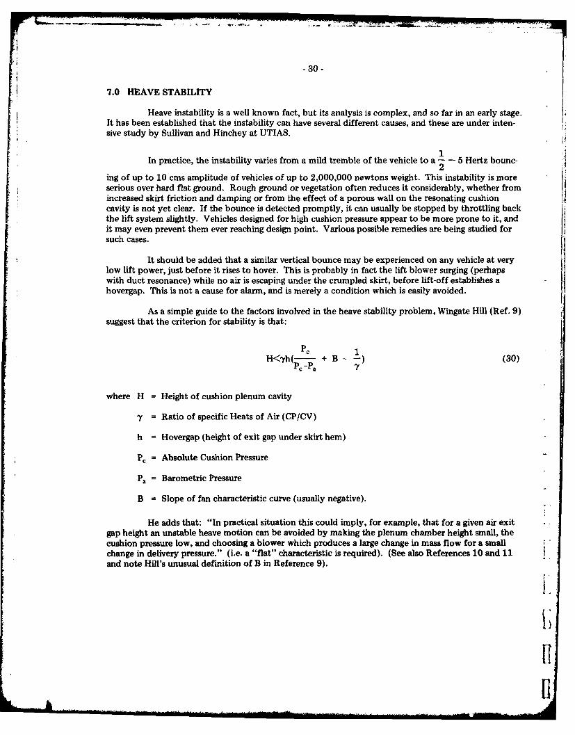
As a simple guide to the factors involved in the heave stability problem, Wingate Hill (Ref. 9)suggest that the criterion for stability is that:

Pc 1H<,yh(- + B-- (30)

PC -P.

where H = Height of cushion plenum cavity

y = Ratio of specific Heats of Air (CP/CV)

h = Hovergap (height of exit gap under skirt hem)

PC = Absolute Cushion Pressure

Pa = Barometric Pressure

B = Slope of fan characteristic curve (usually negative).

He adds that: "In practical situation this could imply, for example, that for a given air exitgap height an unstable heave motion can be avoided by making the plenum chamber height small, thecushion pressure low, and choosing a blower which produces a large change in mass flow for a smallchange in delivery pressure." (i.e. a "flat" characteristic is required). (See also References 10 and 11and note Hill's unusual definition of B in Reference 9).

I

[1

I -31-

S 8.0 A SIMPLE LOW-SPEED ANEMOMETER

A simple anemometer for measuring airspeeds of up to about 15 m/s has been devised andreported by the Von Karman Institute in Brussels, (Ref. 12). It depends on the drag of a sphere, which

S is well known, and on the fact that an ordinary table-tennis ball is a sphere of very closely controlledweight, diameter, and sphericity. Such a ball is hung on about 25 cms of fine flexible thread, and willattain steady equilibrium in a light wind as shown in the attached diagram. It is held well away fromthe observer, in line with a protractor levelled by a spirit level, and the wind-speed may be read off atonce.

80°

600

II I orJ0 0 Ii ~ I / II I o r

Cf I, : i

460

4 VERTI AL

200

000

0, , i ii •

0 1 2 5 4 5 6 7 8 9 0 I: 12 13 14 15rn/s

FIG. 19: V.K.I. LOW-SPEED ANEMOMETER

-32-

9.0 RATE OF FALL OF SPHERICAL PARTICLES

In connection with calculations on dust clouds generated by ACVs, and the inertia-separationof particles in air intakes, it is useful to know the terminal velocity of small particles in air. In clouds,the "downward acceleration" is that due to gravity, while in a centrifugal separator the local centrifugalacceleration should be used. The attached nomogram is drawn for the gravity case, at standard airdensity (2880K, 101.3 kPa), but other cases may be calculated from the formula. The particles areassumed to be spherical. Particles of other forms are likely to fall at lower speeds, with flat thin plate

1particles having a much lower rate of fall, as low as perhaps - the rate of the spherical particle.

3

RATE OF FALL OF SPHERICAL PARTICLES IN AIR

Stokes Law

1 gd2 (Wp - Wa)V = - (31)18 S

V = Velocity of fall cms/sec

g = 981 crns/sec 2

d = Particle diam. cm

Wp = Sp. Gr. particle

Wa = Sp. Gr. air

S = Viscosity of air

181 X 10-6 centipoise

(1 Micron = 0.001 cm)

-v

.1 -33.li

SPECIFIC GRAVITY OF PARTICLES

_-

0 '0?IIIp l a I I ~ I I pI ,iIl l i i.I

NOMOGRAM FOR PARTICLEFALL RATE

AT 2880K AND 101.3 kPa(AFFECTS WA AND S)

RATE OF FALL(CMS/SEC)

0 0 - 0 0 0 -0 0 o0 0

1 Ii I i I lulil I I I I IiiIl I i lill I I ii ,,,l i , liitl I I

PARTICLE DIAMETER(MICRONS)

0 0 0

FIG. 20: RATE OF FALL OF SMALL SPHERICAL PARTICLES IN AIR

*1

-34-

10.0 EFFECT OF ALTITUDE AND TEMPERATURE ON PERFORMANCE

In order to focus attention on the importance of accounting for the atmospheric conditions* of actual operation in design calculations, the performance of an ACV at standard-day sea level condi-

tions, sea level arctic conditions, and at hot-day prairie ground-level altitude has been calculated. Asummary of calculations follows, assuming the same engine and fans in each case.

The vehicle is as follows: Total Weight = 100,000 N (W)Cushion Press. 4000 Pa (Pc)

Cushion Areas 25 m 2 (Sc)

Aspect Ratio = 2:1 (A.R.)V = 7.072 mb = 3.536 mL = 21.216 m

Lift Air Escape CD = 0.61

Lift Airflow = Qm 3 /s (Q)Hoverheight (Standard day) = 0.03 m(h)

Frontal Area = 10.5 m2 (Af)

10.1 Standard Day, Sea Level

p = 1.23 kg/r 3 , t' = 2880 K, Bar = 101.3 kPa.

/P~d X t°K

Lift air exit velocity (from Ve = 0.756Bar

where Pd = Exit dynamic pressure, equal to Pc, in pascals,

to = Atmospheric temp. in OK

Bar = Barometric press., in kilopascals

"Ve = 80.0 m/s

Hence, for 0.03 m hovergap, 21.3 m perimeter, CD = 0.61.

Lift air flow Q = 31.16 m 3 /s

Compressor Power to supply this air, at 70% compressor efficiency and 80% duct efficiency:

Q ApPower - 10cd = 223 kw1000 '?,c ?d

This is assumed to be full power at this condition from the lift engine.

The Total Drag at 20 m/s over smooth deep water, calculated in the standard manner, usingan aerodynamic drag coefficient of 0.36 is

DD Daero + Dmom + Dwave + Dspray + Dskirt

= 1300 N + 460 N + 17000 N + 3100 N + 4200 N 26060 N.

To drive this at 20 m/s would require (at 100% propulsion efficiency)

.35-

U 26000 X 20Power = = 520 kw

* 100

Using a 3 m diam. ducted propeller, of disc area 7.07 m2 , .. Disc loading = Thrust/Area = 3677 N/rm2

at which about 28 N/kw might be expected (from the chart in the section on Thrust).

26000Therefore - = 930 kw would be required at the prop. shaft. This is assumed to be full engine

power from the thrust engine at this condition.

10.2 Recalculation for Arctic Sea Level Condition

t = -40 0 C (= 2330K) Bar = 101.3 kPaHence p = 1.52 kg/m 3

.'. Ve is recalculated (owing to new air density) at 72.5 m/sHowever, Lift Engine Power is proportional to air density, at constant RPM.

Available Lift Power = 275 kwLift Airflow Q (at same efficiency) = 39.0 m3 /s

Therefore Hovergap = 0.0414 mi.e. the hovergap has increased from 3 cms to 4.14 cms.

For a given propeller, thrust is proportional to air density, and engine power will rise in the same ratio288

to drive it, both being considered at constant RPM, so that thrust will rise in the ratio - = 1.236.

Drag, as itemized above will be sensitive to density2 for the aerodynan.i,: drag, density' formomentum drag, and not sensitive for the other components. Since these drags are relatively small,and since the rise of hoverheight will probably reduce skirt drag, the craft speed might bp ,,xpected torise a little.

10.3 Recalculation for Hot-Day at 1067 m Altitude (= 3500 ft. = Calgary)

t" = +35 0 C (= 3080 K) .*. with altitude effect, p = 1.01 kg/m 3

•.Vexit = 89 m/sLift Engine Power = 183 kwand Lift Q = 24.4 m3/sHovergap = 0.021 m

i.e. Hovergap has reduced from 3 cms standard to 2.1 cms.

For a given propeller, the thrust will fall (at const. RPM) to some 0.82 of standard value, and while thedrag will fall slightly, the speed will probably fall off to an appreciable extent.

In a Low Speed Overland Case, where the total drag is believed to be proportional to thehovergap, the drag and engine power will change in opposite senses, so that the Arctic case will showreduced drag and higher power, while the Hot Highlevel case will show increased drag and reducedpower, which will certainly reflect on slope-climbing ability, even with wheel or track propulsion. Itis also likely that there will be a noticeable change in stability of the ACV due to the changes in hover-gap and lift airflow.

- 36 -

11.0 TERMINOLOGY AND NOTATION

11.1 Terminology Peculiar to ACVs, Primarily Overland or Amphibious

Term Definition

apron A sheet of flexible material external to all other skirt compo-nents to suppress spray or dust.

aerodynamic yaw angle Angle in the horizontal plane between the craft C and relativeair direction.

air gap (local) Distance below the local skirt hem and the surface when on itscushion.

bounce An instability in heave which may be involuntary due to aninternal aerodynamic problem, or which may be induced byincreasing lift air supply excessively. Sometimes called tramp-ing.

buzz An involuntary stable oscillation of a bag skirt due to resonance.May be eliminated by adjusting the mass distribution of theskirt material.

anti-bounce web Tensioned skirt membrane connected between upper and lowerbag points to restrain self-sustained vibration, i.e. "bounce".

bag An enclosed inflatable flexible structure supplied with air essen-tially direct from the lift fan. May be used for several purposes.

Peripheral bag - a bag attached to the periphery of the vehicle.May be used as a single skirt component or in conjunction withstern bags (q.v.) to contain and feed the cushion, and also incombination with fingers (q.v.).

Keel bag - a bag dividing the cushion in a fore and aft directionto provide stability in roll.

Stability bag - a bag dividing the cushion in an athwartshipsdirection to provide stability in pitch.

Stern bag - a bag used to seal the cushion at the stern of avehicle; used in conjunction with a peripheral bag. May be usedin combination with cones.

Chip bag - a segment usually at the rear of a craft having an -

additional wall on the cushion side to prevent water scooping.

beam-on Beam-on implies that the craft is travelling sideways, i.e. at a900 angle of yaw to the long axis.

boating Expression used to describe a hovercraft when operating in thewholly displacement condition, i.e. well below hump speed.

centre of pressure Point through which cushion pressure acts vertically to supportvehicle.

J[

I- 37 -

* Term Definition

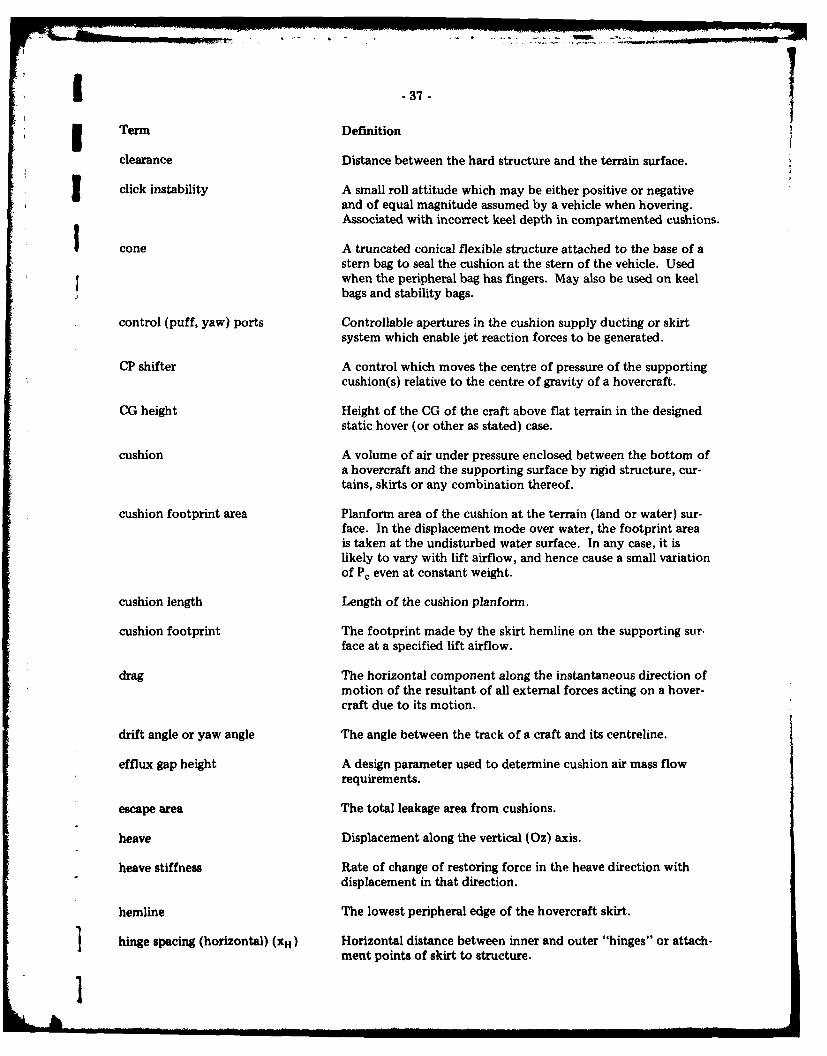
clearance Distance between the hard structure and the terrain surface.

click instability A small roll attitude which may be either positive or negativeand of equal magnitude assumed by a vehicle when hovering.Associated with incorrect keel depth in compartmented cushions.

cone A truncated conical flexible structure attached to the base of astern bag to seal the cushion at the stern of the vehicle. Usedwhen the peripheral bag has fingers. May also be used on keelbags and stability bags.

control (puff, yaw) ports Controllable apertures in the cushion supply ducting or skirtsystem which enable jet reaction forces to be generated.

CP shifter A control which moves the centre of pressure of the supportingcushion(s) relative to the centre of gravity of a hovercraft.

CG height Height of the CG of the craft above flat terrain in the designedstatic hover (or other as stated) case.

cushion A volume of air under pressure enclosed between the bottom ofa hovercraft and the supporting surface by rigid structure, cur-tains, skirts or any combination thereof.

cushion footprint area Planform area of the cushion at the terrain (land or water) sur-face. In the displacement mode over water, the footprint areais taken at the undisturbed water surface. In any case, it islikely to vary with lift airflow, and hence cause a small variationof P, even at constant weight.

cushion length Length of the cushion planform.

cushion footprint The footprint made by the skirt hemline on the supporting sur.face at a specified lift airflow.

drag The horizontal component along the instantaneous direction ofmotion of the resultant of all external forces acting on a hover-craft due to its motion.

drift angle or yaw angle The angle between the track of a craft and its centreline.

efflux gap height A design parameter used to determine cushion air mass flowrequirements.

escape area The total leakage area from cushions.

heave Displacement along the vertical (Oz) axis.

heave stiffness Rate of change of restoring force in the heave direction withdisplacement in that direction.

hemline The lowest peripheral edge of the hovercraft skirt.

hinge spacing (horizontal) (XH) Horizontal distance between inner and outer "hinges" or attach-ment points of skirt to structure.

I

-38-

Term Definition

hinge spacing (vertical) (z H ) Vertical distance between inner and outer "hinges" or attach-ment points of skirt to structure.

hump speed A speed over water at which there is a peak value of the wave-making drag. In general there will be several hump speeds, thehighest being known as the "primary hump speed".

hydrodynamic yaw angle The angle, in the horizontal plane, between the longitudinal axisof a hovercraft and the instantaneous direction of motionrelative to the local water surface.

loop An abbreviated form of bag having large openings over the seg-ments so that there is little pressure difference between the loopand the cushion. A loop may or may not include a sheet ofmaterial inboard of the segment inner attachments. N.B. Thereis no definitive demarcation as to when a bag becomes a loop.

mean bag or loop pressure Mean pressure in bag or loop, relative to atmospheric pressure.

nibbling The action describing the catching of the skirt, usually the bowfingers, on the surface being traversed. Nibbling is one indica-tion of a possible plough-in situation developing.

pitch attitude Instantaneous angle between the surface traversed and the longi-(roll attitude) tudinal (lateral) datum of the craft.

pitch stiffness Rate of change of restoring pitching moment with pitch angle.

plenum Space or air chamber beneath or surrounding a lift fan or fanxs(not to be confused with "cushion").

plough-in A divergent pitching motion involving an increase in drag andnose-down pitch attitude.

propeller fin effect The propeller lateral force (normal to the axis of rotation)which results from a side gust.

puff ports See "control ports".

hoverheight or rise height The distance which a hovercraft rises from flat hard ground tobeing fully cushion-borne.

roll stiffness Rate of change of restoring rolling moment with roll angle.

rough water drag increment The increment in the hydrodynamic drag during operation inrough water over the drag (under otherwise identical conditions)in calm water, taken as a time average.

SKIRT SYSTEMS

Term Definition

bag A skirt system in which cushion containment is effected only bya bag or bags. Generally restricted to small recreational vehicles.

.. . . .. t tt I .. ... ..... .. ... .. .. . .. .... [.

-39-

Term Definition

bag-and-finger A skirt system in which cushion containment is effected by abag or bags with fingers attached. This system is occasionally*referred to as the "BHC system" since it is the commonly usedsystem on BHC-designed vehicles. The cushion contained bythis system generally requires keel and stability bags for stability.The cushion is fed through feed holes from the bags, and fromthe fingers.

Bertin A skirt system employing an array of jupes to supply cushion airand stabilize the vehicle. This jupe is often enclosed within aperipheral skirt. So called due to its origin with the Frenchdesigner Jean Bertin, whose vehicle designs use it exclusively.

loop/segment A skirt system in which the cushion containment is effected bya loop and segments. This system is occasionally referred to asthe "HDL system" since it originated and was developed byHovercraft Development Ltd. (HDL). The cushion is generallya simple plenum with no compartmentation.

peri-cell A peripheral array of small diameter jupes used to contain acushion. Sometimes referred to as peri-jupe.

flexi-cell An array of shallow jupes attached to a horizontal flexible dia-phragm which forms the base of a plenum beneath the vehicle.

feed hole A hole, usually circular, cut in bag or segment to allow flow ofcushion air. May be used in peripheral and stern bags, or insegments. May also be used in keel and stability bags to stabi-lize their inflated shape.

finger A sheet of flexible material attached to the lower surface of aperipheral bag to seal the cushion. Fingers are generally open onthe inboard side, and are fed with air from feed holes in the bag;they are generally closed at the top by the bag.

jupes Truncated conical inflated flexible structures, generally used inmultiplicity to feed air into the cushion of a vehicle using aBertin skirt system.

segment One of a series of sheets of flexible material attached to a loopand the underside of the vehicle to seal the cushion. A segmentis open at the top, fed with air either from the loop or thecushiot plenum, and may be open or closed on the inner face.Feed I oles are sometimes cut in the inner face if this is closed.

segment angle The angle between the outer face of a segment and the surfaceof the ground.

skirt height (HsK) Designed vertical distance from the craft hard structure to fingertip. See Figure 31.

stability skirt (trunk) A skirt used to divide a cushion to increase the pitch or rollstability by preventing or restricting cross flow.

surge Displacement along the longitudinal (Ox) axis.

-40-

Term Definition

sway Displacement along the lateral (0y) axis.

tip flip Turning-under of the lower tip of a segment or finger.

track The direction of the path of the craft over the earth.

trim angle (longitudinal) The pitch or roll angle which results under steady running(lateral) conditions.

tuck-under The action of the skirt being pulled back under the structure as

a result of local drag forces.

(94

CO-ORDINATE SYSTEM

N.B. POSITIVE DIRECTIONS OF MOTION AS FOLLOWS:

TRAVEL - FORWARD - +SURGE - FORWARD - +SWAY - TO STARBOARD (RIGHT) - +HEAVE - DOWNWARD a +ROLL - STARBOARD DOWN - +PITCH - STERN DOWN - +YAW - BOW TO STARBOARD - +

FIG. 21: ACV COORDINATE SYSTEM

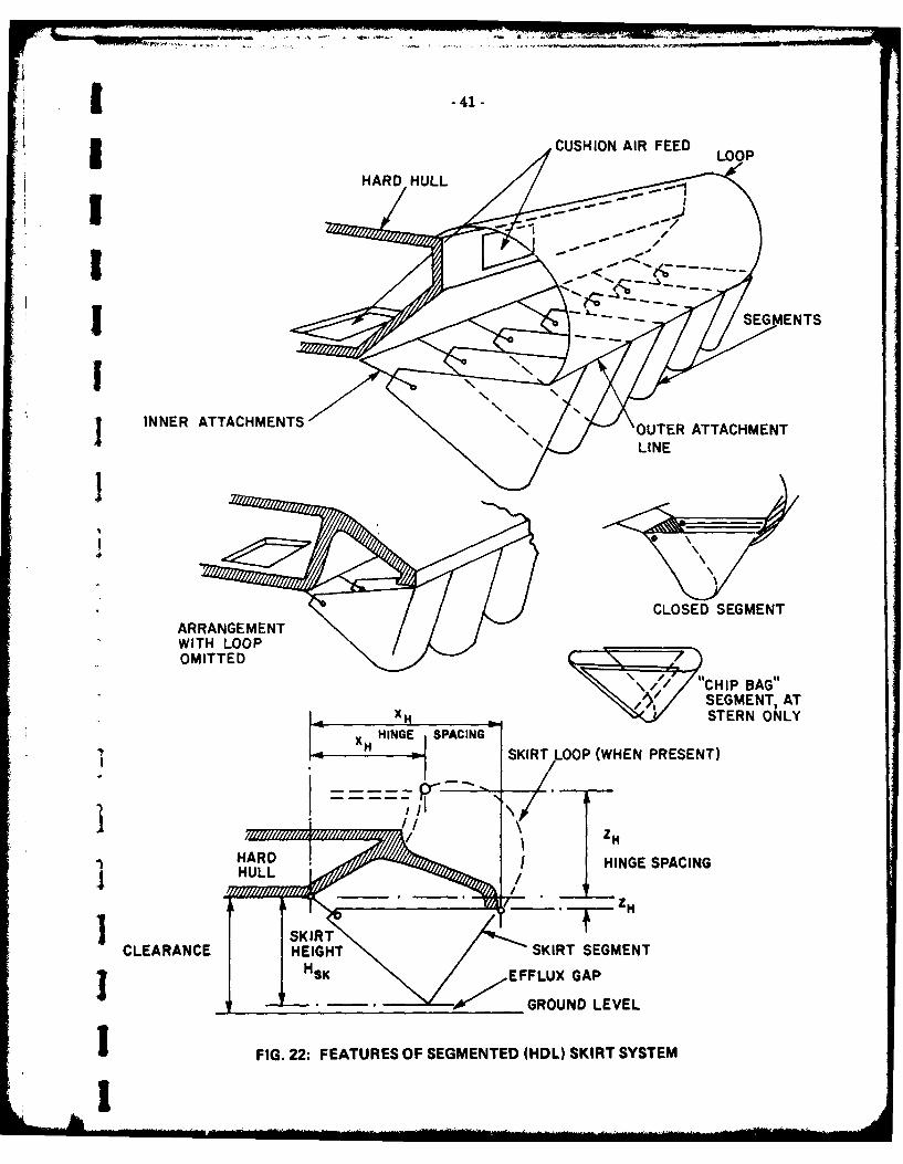
..1 -41-

CUSHION AIR FEED OO

~HARD HULL

Ij

J INNER ATTACHMENTS

LINE

ARNEETCLOSED SEGMENTARRANGEMENTWITH LOOPOMITTED "-7

"CHIP BAG"M SEGMENT,AT

H -STERN ONLYxHINGE ISPACING

SKIRT LOOP (WHEN PRESENT)

iiHHARDI HINGE SPACINGHULL/

SR ZH

CLEARANCE HEIGHT SKIRT SEGMENT1' HSK j EFFL.UX GAP

__ __ __ __ GROUND LEVEL

1 FIG. 22: FEATURES OF SEGMENTED (HDL) SKIRT SYSTEM

: I

-42-

PLENUJM

CHAMBSIER

OUTER SKIRTUOYA~c

'__) 0 OUTER SKIRT0 0 -0 FEED HOLES

CUSHION 0 ANTI- BOUNCEFEED HOLES 4"WES

INNER SKIRT " 0

FINGER FEED HOLES 0AR

FIG. 23: FEATURES OF FLEXIBLE TRUNK AND FINGER (BHC) SKIRT SYSTEM

b.

S/ ,LIFT FAN

AIRTIGHT BULKHEADON (L SEPARATING PORTJ AND STARBOARD LIFTAIR PLENUMS

/ PERIPHERALSKIRT SKIRT

DELECOAIR FEED HOLESA ETO JUPES

--- _ j JUPES

SINGLE CELL ("JUPE")TATTACHMENT DIAM. _I.

SKIRTHIGH

" -FAN DELIVERIES PLENUM

GROUNDIN CUSIO PRESSURE

TAFEED JET PLENUM SKIRTDEFLCTORFEED HOLESDEFLE TOR IPLEI

TOTAL CONEr/ ," CLANGLECOEEL

PERIPHERAL \ PRESSURE

GROUND CUSHION PRESSURE

: TOTAL FOOTPRINT AREA ENCLOSED BY PERIPHERAL SKIRT

IS COMPOSED OF SUM OF CELL FOOTPRINT AREAS PLUS

REMAINING "CUSHION AREA".

FIG. 24: FEATURES OF BASIC MULTICELL (BERTIN) SKIRT SYSTEM

V

:1 -44-

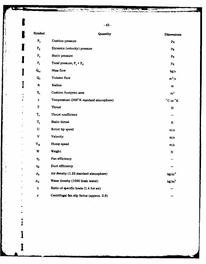
11.2 Notation

Symbol Quantity Dimensions

A Frontal area m2

A e Escape area (=Efflux gap height X cushion perimeter) m2

b Cushion footprint beam m

CD Coefficient of discharge

CD A Aerodynamic drag coefficient

D Diameter m

DA Aerodynamic drag N

DH Wavemaking drag at hump speed N

DM Inhaled-air momentum drag N

DSF Skirt-friction drag N

DST Skirt-terrain interaction drag N

Dsp Spray drag N

Dw Wavemaking drag N

FN Froude number V/V

g Acceleration due to gravity (9.81 m/s 2 ) m/s2

h Efflux gap height ("Hovergap") m

hf Efflux gap height over flat nonporous ground at low speed m

H Hoverheight (Vertical rise of vehicle from rest to hovering position (Approx.equal to skirt height + efflux gap height) m

K Efflux gap height Terrain and Operational factor

L Cushion footprint perimeter, f 2(k+b) m

2 Cushion footprint length m

RC Cushion footprint effective length, = S,/b m

M n Mach number (V/Vsound)

M Mass kg

PA Barometric pressure (101.3 kPa standard) Pa

Pb Bag pressure Pa I.

S- 45-

5 Symbol Quantity Dimensions

PC Cushion pressure Pa

IPd Dynamic (velocity) pressure Pa

PS Static pressure Pa

Pt Total pressure, Ps + Pd Pa

J Qm Mass flow kg/s

Qv Volume flow m3/s

R Radius In

Sc Cushion footprint area m 2

t Temperature (2880 K standard atmosphere) 0 C or OK

" T Thrust N

Tc Thrust coefficient

Ts Static thrust N

U Rotor tip speed m/s

V Velocity m/s

VH Hump speed m/s

W Weight N

17C Fan efficiency

7?d Duct efficiency

Pa Air density (1.23 standard atmosphere) kg/rm3

Pw Water density (1000 fresh water) kg/m 3

7 Ratio of specific heats (1.4 for air)

a Centrifugal fan slip factor (approx. 0.9)

i1I

-46.

12.0 REFERENCES

1. Fowler, H.S. The CASPAR ACV Research Project Report No. 3, On the Drag ofA CVs Overland.NRC Associate Committee on Air Cushion Technology, TechnicalReport No. 1/75. 1975.

2. Fowler, H.S. The CASPAR ACV Research Project Report No. 6, The use of aquantitative description of lift airflow applicable to any ACV.NRC Associate Committee on Air Cushion Technology, TechnicalReport No. 1/78. 1978.

3. Fowler, H.S. The Lift Air Requirements of ACVs over Various Terrain.Proceedings of the Annual Air Cushion Technology Symposium ofthe Canadian Aeronautics and Space Institute (Toronto, October1978).

4. Fowler, H.S. Thrust Systems for Light Air Cushion Vehicles.NRC Associate Committee on Air Cushion Technology, TechnicalReport No. 1/74.

5. Trillo, R.L. Marine Hovercraft Technology.Leonard Hill Books Ltd., London 1971.

6. Mantle, Peter J. A Technical Summary of Air Cushion Craft Development.David W. Taylor Naval Ship Research and Development Centre,Maryland, U.S.A., Report 4727, 1975.

7. Elsley, G.H. Hovercraft Design and Construction.Devereux, A.J. David and Charles Ltd., Newton Abbot, UK, 1968.

8. Fowler, H.S. The CASPAR ACV Research Project Report No. 4, Program 1, TheMulticell Skirt, a Summary.NRC Associate Committee on Air Cushion Technology, TechnicalReport 5/76. 1976.

9. Wingate Hill, R. A Tracklaying Air Cushion Vehicle.Journal of Terramechanics, 1975, Vol. 12, No. 3/4, pp. 201-216.

10. Sweet, L.M. Linearized Models, Stability Criteria, and Experimental VerificationRichardson, H.H. for Plenum A ircushions with Compressor-Duct Interactions.Wormley, D.N. Massachusetts Institute of Technology, Dept. of Engineering, 1974.

11. Hinchey, M.J. Effect of Ducting in the Heave Stability of Plenum Air Cushions.Sullivan, P.A. Journal of Sound and Vibrations (to be published, 1978).

12. Clemens, P.L. An aerodynamic pendulum of standard design and simple con-struction for verification of anemometer calibrations at lowvelocities.Von Karnan Institute Technical Memo, No. 22, May 1971.

. ..... 3

*i -47-

13.0 SI UNITS AND IMPERIAL EQUIVALENTS

In the following pages, the SI units for quantities most often used in ACV technology arestated, and their Imperial equivalents are given to normal engineering standards of accuracy. In mostcases a graph is also given for quick approximate conversion.

Note on the Relation Between Mass, Weight and Force

The common confusion between the terms "Mass" (of an object, measured in kilograms) and"Weight" (the downward force exerted on the same object in the earth's gravitational field, measuredin newtons) has caused engineers trouble ever since Newton invented gravity. These pages, dealingwith an unfamiliar system of units, therefore seem a good place to remark on the relation between theunits of Mass and Force in this system.

The quantity of matter in an object is the measure of the force necessary to give it a stated

acceleration. This quantity of matter in an object, i.e. the mass of the object, is measured in kilogramsin SI units.

The force needed to generate a stated acceleration in the object is measured in newtons in SIunits.

When an object is held in the hand, the downward force exerted by it under the influence ofthe earth's gravitational field, is called its weight, but being a force it must properly be expressed innewtons.

The newton is defined as the force required to give a mass of I kilogram an acceleration of 1metre per second per second. Since the earth's gravitational field produces an acceleration of 9.81 m/s2

at standard seal level conditions, the weight of an object whose mass is I kilogram is equal to 9.81 new-tons.

In ACV calculations the mass of the vehicle and its components must often be specified,when concerned with its acceleration in various directions under various forces. The vehicle totalmass, and component masses, are therefore specified in kilograms.

However, the vertical downward force exerted by the vehicle on its air cushion, commonlyknown as its "weight", being a true force, must be expressed in newtons. The value of this "weight"in newtons will be numerically equal to 9.81 times its mass in kilograms.

It then becomes simple to equate the downward force (weight) of the vehicle in newtons, tothe upward supporting force of the air cushion in units of pressure X area, (newtons/metres2 ) Xmetres2 , which is clearly a force in newtons.

Any other force experienced by the vehicle in a turn or in transient motion is equallyproperly expressed in newtons, provided the mass in kilograms is known, and that the acceleratior canbe specified in m/s2 . The commonly used acceleration stated as so many" ust therefo

pressed as so many times 9.81 m/s2 (e.g. 5g becomes 5 X 9.81 = 49.1 m/s 2 ).

Units of Pressure

The standard SI unit of pressure is the pascal - which equals one newton per square metre,in conformity with the discussion above. However, an optional unit which is more convenient to thepressures used in ACV technology is the water-gauge pressure, stated in cm of water. The equivalenceis approximately 1 cm water = 100 pascals.

Units of Power

Since Work = Force X Distance Moved

Work unit 1 1 newton X 1 metre - 1 watt second 1 1 joule

|I

-48-

WorkAnd since Power = -

Time'

newton metresthe power unit = = watts.

seconds

Or, more conveniently,

newtons X metres =kilowattsseconds X 1000

[in conversion, 0.746 kw 1 Horse Power, or I kw = 1.34 HP.]

I.

1 -49-

14.0 ACKNOWLEDGEMENT

These data have been compiled, and in some cases generated, under the CASPAR program,operated by the National Research Council of Canada, and partially supported by grants from TransportJ Canada, (Transportation Development Centre and ACV Division, Canadian Coast Guard), and from theDefence Research Board. The writer also wishes to acknowledge the generous assistance in compilingthis handbook given by Mr. R. Dyke, Dr. P.A. Sullivan, and Mr. R.G. Wade.

1~

- 50 -

Lu5

I-

0 5 10 15 20 25 30FEET (f t.)

10

1.0 M 2 = 10.80 ft2 III

w

05-- 1111 --- -----

FET (t2)8

AREA CON.0IOIEi l f l

00 0 20 30 0 40 100

FEET (f)i

FIG.... 25:. LEGH.RA.ADVLMECNESO

I ' l l I l I f

-51-

1.0 Pounds =0.4536 Kilograms

100 . Kioras 2.00 Pou20d2

Kilogams g nwton

000z 01 02

PONS,.Os

150

Jil

- 52 -

_40 - I310I I f l

300

300

20

290 00

L0I'AW

0 y

0280 cn

- J I F r e e z e p o i n t o f w a t e r- -- - - -

>

iLJ 00

270

260

250 vII1

-10 0 +10 +20 .30 40 50 60 70 80 90------- FAHRENHEIT

450 460 470 480 490 500 510 520 530 540 5500 RANKINE (ABSOLUTE)J

FIG. 28: TEMPERATURE CONVERSION

-53-

INCHES OF WATERGAUGEO 10 20 3

S1.0 kPa =0. 145 psi -- T wE--

z 3 60N- 6X10

3

-F-

O4x 103 14044 13

w Lz0

a_ L)

4 2 03 20

.40..

O 0.2 0.4 0.6 0.8 1.0

INS Water x 249 =Pa

C~MS Water X 98 =Pa

INS Mercury x 3386 Pamm Mercury x 133.3 PaPSF x 47.88 -PaMillibars x 100 = Pa

Standard Atmosphere 101.3 x 103 PSa 1013.0 mb=760 mm Mercury=14.696 psi29.92 inches Mercury - 406.9 inches water

- 1033.55 ems water.

FIG. 29: PRESSURE CONVERSION

-54.

1.6

E Air density, Sea level, Standard day~I4288 0K 1013 mlb ---

w-L -l

w

0-j

0.80.06 0.07 POUNDS/FT 3 0.08

FIG. 30: AIR DENSITY VALUES AND CONVERSION

AIR DENSITY AT STANDARD SEA LEVEL ATMOSPHERE [2880K, 1013 mb]

= 1.230 kg/rn 3 = 0.07652 lbs/ft3 -0.00238 slugs/ft3

AIR DENSITY AT OTHER TEMPERATURE AND PRESSURE t0K and P mb

- 1.230 x 28 x -

t 1013

-0.350 - X kg/rn3.t T'

1 -55-

----------4I

II t I

F II I

II'L

4 + ---- L

10

0007-

0 1 L0

l T- 12x 1eon - Fio ats 1 1111 jII

FIG.32: OWERCONVRSIO

-TTT I -II I I I Loo

-j I I I I I I L i.

--0 in 1. 1 - 1 7

1 -57-

I25 I

1

II I I I !LL

-1.0 ft3/sec = 0.0284 m 3/sI

S"I1.0 m /s= 35.32 ft3/secz III

20

E I

Z 150

w

5

APPROXIMATE DISCHARGE COE FF ICIENTS:

1(a) SHARP EDGED ORIFICE Co = 0.61(ALSO BETWEEN BHC. HDL AND BERTIN TYPE SKIRT HEMS AND FLAT SMOOTH GROUND)

3(b) BELL MOUTH Cc) - 0.98

(INHALING FROM LARGE VOLUME OF STILL AIR)

(c) BAG SKIRT EFFLUX OVER SMOOTH CD -09

FLAT GROUND (ESTIMATED).

II

0 z 0

~ eq

zz'-C Eo* ; 9 -'*

~ 'w .0 lc

od >*0z Cz 0

0 C- 0 .0C. ~ ~ C

~C ~ .~ 1wC

0 Dr *z' 0E P

~ ~! ~ ~2cW ~~~1

All. 9r