Ad Hoc Networks 9 (2011) 341–354

Contents lists available at ScienceDirect

Ad Hoc Networks

journal homepage: www.elsevier .com/locate /adhoc

G-STAR: Geometric STAteless Routing for 3-D wireless sensor networks

Min-Te Sun a,*, Kazuya Sakai b, Benjamin R. Hamilton c, Wei-Shinn Ku b, Xiaoli Ma c

a Department of CSIE, National Central University, Taoyuan 320, Taiwan, ROCb Department of CSSE, Auburn University, Auburn, AL 36849, United Statesc School of ECE, Georgia Institute of Technology, Atlanta, GA 30332, United States

a r t i c l e i n f o

Article history:Received 15 February 2010Received in revised form 20 July 2010Accepted 27 July 2010Available online 10 August 2010

Keywords:Geometric routingWireless sensor networks3-Dimensional networks

1570-8705/$ - see front matter � 2010 Elsevier B.Vdoi:10.1016/j.adhoc.2010.07.013

* Corresponding author. Tel.: +886 3 422 7151; faE-mail address: msun@csie.ncu.edu.tw (M.-T. Su

a b s t r a c t

3-D aerial and underwater sensor networks have found various applications in natural hab-itat monitoring, weather/earthquake forecast, terrorist intrusion detection, and homelandsecurity. The resource-constrained and dynamic nature of such networks has made thestateless routing protocol with only local information a preferable choice. However, mostof the existing routing protocols require sensor nodes to either proactively maintain thestate information or flood the network from time to time. The existing stateless geometricrouting protocols either fail to work in 3-D environments or have tendency to producelengthy paths. In this paper, we propose a novel routing protocol, namely Geometric STAte-less Routing (G-STAR) for 3-D networks. The main idea of G-STAR is to distributively build alocation-based tree and find a path dynamically. G-STAR not only generalizes the notion ofgeographic routing from two modes to one mode, but also guarantees packet delivery evenwhen the location information of some nodes is either inaccurate or simply unavailableregardless of the uses of virtual coordinates. In addition, we develop a light-weight pathpruning algorithm, namely Branch Pruning (BP), that can be combined with G-STAR toenhance the routing performance with very little overhead. The extensive simulationresults by ns-2 have shown that the proposed routing protocols perform significantly bet-ter than the existing 3-D geometric routing protocols in terms of delivery rate with com-petitive hop stretch. We conclude that the proposed protocols serve as a strongcandidate for future high-dimensional sensor networks.

� 2010 Elsevier B.V. All rights reserved.

1. Introduction

3-D wireless sensor networks (WSNs), such as under-water acoustic sensor networks [1] and aerial networks[2], are a special type of wireless networks, which has vastapplications in natural habitat monitoring, weather/earth-quake forecast, terrorist intrusion detection, and homelandsecurity [3]. The resource-constrained and dynamic natureof such networks, such as nodes have limited memory andinaccurate local information, has made the design of 3-Drouting protocols complicated. Compared with the tradi-tional proactive [4] and reactive [5] routing protocols, geo-metric routing [6–9] is more suitable as it only uses the

. All rights reserved.

x: +886 3 422 2681.n).

local location information to deliver packets with low com-munication and storage overheads. In most geometricrouting protocols, there is no need for nodes to maintainglobal state information nor flood the network in searchof a path to the destination.

In general, for many existing geometric routing algo-rithms to function correctly, three assumptions are re-quired. First, the location information at each node needsto be accurate. Second, the link model is assumed to bethe unit disk model for 2-D networks or unit ball modelfor 3-D networks, i.e., nodes within a predefined transmis-sion radius can always exchange packets with each other.Last, the network topology needs to be on a 2-D plane. Inpractice, it is difficult to obtain accurate location informa-tion at each node regardless of what localization algorithmis used. The protocols that assume the unit disk model or

342 M.-T. Sun et al. / Ad Hoc Networks 9 (2011) 341–354

unit ball model can result in very poor performance in real-ity [10]. In addition, nodes in many WSNs are deployedover 3-D space such as aerial networks and underwaterwireless sensor networks. As a result, these assumptionsrender most of the existing geometric routing protocolsunusable for 3-D WSNs.

To do away with the aforementioned assumptions, anumber of effort have been made. The geometric routingprotocols proposed in [11,9,12,13] are able to relax someof these assumptions, but they either produce lengthypath, introduce heavy communication overhead, or requireeach node to proactively maintain routing information. Onthe other hand, routing with virtual coordinates [14,15]has been proposed for the locationless networks. In[14,15], nodes in the network set up their virtual coordi-nate by using centroid transformation. 3RuleGeo protocol[16] routes a packet by traversing unvisited nodes basedon the constructed virtual coordinate by using PathRecording [17]. VRR [18] and VCP [19] use a distributedhash table (DHT) to create an overlay network topologyin ad hoc networks. In such a virtual topology, greedy strat-egy always works, and so packets are forwarded to thenode closest to the destination in the virtual topology.Although these protocols work in the network where loca-tion information is not available or inaccurate, additionaloverhead is required to set up virtual coordinates or anoverlay network topology.

In this paper, we propose a novel geometric routingprotocol, namely Geometric STAteless Routing (G-STAR).The main idea of G-STAR is to distributively build a loca-tion-based tree and find a path dynamically. G-STAR hasthe following preferred properties:

� G-STAR is stateless: Unlike GDSTR [9], the prioritizedDFS [20,21], and GHG [13], no state information is pro-actively maintained at each node in G-STAR.� G-STAR runs in one mode: In most of the geometric

routing protocols, there are more than one mode, suchas the greedy mode and the detouring mode, when apacket is routed toward its destination. Using onlynext-hop selection criterion, there is no need for G-STAR to switch between modes or perform networktopology planarization.� G-STAR guarantees packet delivery even when the loca-

tion information at some nodes is inaccurate or missing.Unlike [14–19], G-STAR does not rely on the availabilityof virtual coordinate.� G-STAR can be combined with the Branch Pruning algo-

rithm (BP), a light-weight algorithm which effectivelyremoves the loops in the path with small overhead.� G-STAR is compatible with the concept of virtual coor-

dinates. When the location information is unavailable,G-STAR can route the traffic using virtual coordinatesto further improve the performance.

The extensive simulation results validate that the pro-posed G-STAR routing algorithm significantly outperformsthe existing 3-D geometric routing protocols, such as GRG[12], GHG [13], GDSTR [9], and 3RuleGeo [16].

The rest of the paper is structured as follows. Section 2surveys the related work of geometric routing. Geometric

STateless Routing protocol as well as the Branch Pruningalgorithm are illustrated in Section 3 and the experimentalresults are presented in Section 4. Finally, Section 5 con-cludes the paper.

2. Related work

The traditional wireless ad-hoc routing protocols areclassified into proactive and reactive protocols. In proac-tive protocols, such as DSDV [4], each node periodically ex-changes routing information to maintain a routing table. Inreactive protocols, such as DSR [5], a node floods the entirenetwork to discover a path to its destination whenever ithas a packet to send. While the traditional protocols areable to handle 3-D routing, they result in poor performancein large scale WSNs due to their communication and stor-age overheads.

For large-scale WSNs, geometric routing protocols[7,22,23,8] are known to be light-weight and efficient. Ingeneral, these geometric routing protocols can determinewhere to forward a packet without maintaining a routingtable or flooding the network as long as each node in thenetwork knows the location of itself and its neighbors,and the source knows and encodes the destination locationin the packet. These geometric routing protocols com-monly consist of the greedy forwarding and detouringmodes. In greedy forwarding mode, a node forwards apacket successively to the neighbor closest to the destina-tion. When no closer neighbor to the destination is found,i.e., the local minimum is reached, the packet enters thedetouring mode. Different geometric routing protocol han-dles the detouring forwarding differently. Depending onthe dimension of each node’s location, these geometricrouting protocols are categorize into 2-D, 3-D, and no loca-tion information as follows.

2.1. 2-D geometric routing

GPSR [7] and the face routing family, e.g., AFR [22],GOAFR [23], and GOAFR+ [8] are the most popular 2-D geo-metric routing protocols. The detouring strategy in thiscategory recovers a packet by forwarding it on the planargraph with certain rules to avoid repeated loops. For a gi-ven network topology, several distributed algorithms, suchas GG [24] and RNG [25], are available to planarize a net-work topology. In these algorithms, each node autono-mously eliminates some edges to its neighbors from theconsideration of the detouring routing based on the local-ized information so that the resulting graph does not con-tain cross edges. For example, in the detouring mode ofGPSR, a packet is forwarded successively on closer facesof the planar graph until it reaches the destination or anode closer to the destination than the previous local min-imum, where the packet is switched back to the greedy for-warding mode.

The geometric routing protocols [7,22,23,8] guaranteepacket delivery under the assumptions that all nodes inthe network have accurate location information, the linkmodel is the unit disk, and the network topology is on a2-D plane. However, these assumptions are not available

M.-T. Sun et al. / Ad Hoc Networks 9 (2011) 341–354 343

in real sensor network scenarios. When some of theseassumptions are not satisfied, these protocols either failto deliver the packet or lead to poor routing performance[10].

2.2. 3-D geometric routing

The stateless geometric routing in 3-D networks ismore challenging and difficult than in 2-D networks.There are several works to do away with the aforemen-tioned expensive assumptions. A practical planarizationtechnique, CLDP [10], is proposed to make 2-D geometricrouting work with imprecise location information andgeneral link model. In CLDP, each node periodicallyprobes its neighbor to eliminate cross edges. CLDP is ableto accommodate arbitrary graph and can be applied toGPSR and the face routing family. The geometric routingusing GPSR with CLDP will work on 3-D topologies, butthe performance can drastically decreases on higherdimensional topologies. In addition, CLDP incurs toomuch communication overhead as shown in [9]. In [11],each node is assigned a virtual coordinate in hyperbolicplane and the greedy forwarding is performed with re-spect to these virtual coordinates. However, the evalua-tion of the virtual coordinate is not localized and has tobe updated whenever the topology changes. In GDSTR[9], a spanning tree is constructed for the entire networkand each node makes use of the convex hull of its chil-dren in the tree for routing. There are several drawbacksin GDSTR. First, GDSTR requires multi-dimensional convexhull calculations which would demand significant pro-cessing resources. Second, each node needs to maintaina convex hull for each children, and it introduces highstorage overhead in proportion to the scale of the net-work. Third, if location information is inaccurate, a defec-tive spanning tree will be constructed and routing mayfail. Finally, the spanning tree needs to be reconstructedshould the network topology change, and the overheadto reconstruct the spanning tree is extremely high. Theseprotocols are considered too expensive for 3-D WSNs, asthey commonly incur high control overheads.

In [12], a randomized geometric routing, called GRG, isproposed which consists of the greedy forwarding andrandom walk modes. When a packet reaches the localminimum, the packet is randomly forwarded within thebounded region until it recovers from the local minimum.If the packet is not recovered within a certain number ofhops, the bounded region is extended and the randomwalk is repeated. While GRG is stateless and could be ap-plied to an arbitrary graph, the random walk forwardingcan lead to a long path. In [13], GHG is proposed whichconsists of the greedy forwarding and depth-first search(DFS) modes. In detouring mode of GHG, a packet is for-warded by the prioritized DFS [20,21] along a subgraph,called a hull graph. To obtain the hull graph, it employsPUDT [26] which captures the empty 3-D network sub-spaces to eliminate intersecting triangles and edges fromthe consideration of the DFS. To record visited nodes,each node keeps a routing table by marking visitedneighbors for each destination. Even though GHG is veryeffective in an ideal environment, it does not work well

in reality as PUDT assumes the link model of the unit ballgraph. In addition, as each node has to maintain a routingtable in the prioritized DFS, GHG incurs high storageoverhead.

Although there are several routing 3-D geometric rout-ing protocols, such as DBR [27], DSDR [28], and HH-VBF[29], they are primarily designed for underwater commu-nications. Since our focus in this paper is geometric routingin general 3-D WSNs, we omit special physical constraintsof acoustic communications from our consideration.

2.3. Routing without location information

The aforementioned geometric routing protocol re-quire location information. However, in the real sensornetworks, sensor nodes often do not have their locationinformation or the location information is inaccurate.To handle such environments, routing with virtual coor-dinates are proposed in [14–16]. Since nodes are as-sumed not to have their location information, they firstset up their virtual coordinate. Then, geometric routingis applied based on virtual coordinates instead of reallocation. Rao’s protocol [14] consists of two phase. Inthe first phase, nodes are in perimeter are identified. Inthe second phase, non-perimeter nodes iteratively up-date their virtual coordinate by centroid transformation.In [15], centroid transformation is enhanced by eliminat-ing the first phase of Rao’s protocol. To fully take advan-tage of virtual coordinates, 3RuleGeo geometric routingprotocol is proposed in [16]. Similar to the traditionalgeometric routing, 3RuleGeo protocol consists of thegreedy and perimeter modes. In its perimeter mode,the sequence of already traversed nodes is used to selectthe next hop, which can be achieved by Path Recording[17].

Alternative approach is to construct an overlay networkwith a distributed hash table (DHT), which provide a lookup service in distributed file systems and peer to peer net-works. In [18], VRR is proposed to form a virtual ring toconnect nodes by increasing node identifer across the net-works. Then, a node forwards a packet to the node closestto the destination in ID space. The problem of VRR is thatneighbors in the virtual ring may not be direct neighborsin the real network. The virtual cord protocol (VCP) is pro-posed in [19], in which the adjacent nodes in the virtualcoordinate system are direct vicinity in the real networktopology. Hence, VCP reduces the communication over-head and is more scalable. While routing on virtual coordi-nate can deliver packets in the networks where locationinformation is not available, nodes are required to con-struct virtual coordinates or an overlay network beforerouting can take place.

3. Geometric stateless routing

In this section, we introduce our stateless geometricrouting protocol, namely Geometric STAteless Routing(G-STAR), its properties, implementation considerations,as well as a post optimization technique, called BranchPruning (BP).

344 M.-T. Sun et al. / Ad Hoc Networks 9 (2011) 341–354

3.1. Design goals and network setup

Due to the nature of 3-D WSNs [1,2], an ideal 3-D geo-metric routing protocol must achieve the following designgoals.

� It should allow a node holding a packet to determinethe next hop locally and distributively.� It should be memory-efficient.� It should not assume the model of unit ball graph (cor-

responding to the unit disk graph in 2-D).� It should work even if location information is inaccurate

or missing.

The notations used in the following discussion are listedin Table 1.

To ensure the proposed protocol functions properly,there are three required conditions of the network: (i)the link needs to be bi-directional so that a packet can tra-verse back as needed, (ii) source and destination are con-nected, and (iii) the network topology remains staticduring the routing process. Whether or not a link is bi-directional can be verified by its two endpoints by utilizinga link-layer protocol similar to the three-way handshakescheme in TCP [30]. As for the source-destination connec-tivity condition, since any pair of nodes can be selectedas source and destination, this implicitly requires thatthe network to be connected. The connectivity of a sensornetwork can be verified at the time of network deploymentor be checked by one of localized topology control algo-rithms [31–33], regardless of the network dimension. Thelast condition is commonly assumed by most of the routingprotocols. In fact, no routing protocol can guarantee packetdelivery if the network topology changes fast during therouting process. In summary, these conditions can be ful-filled easily in real-world applications.

3.2. Protocol description

In G-STAR, a node always routes a packet to the neigh-bor closest to the destination as long as no loop is created.To avoid loops, a packet in G-STAR is required to record thepartial network topology it has already exploited. Whilethere are known data structures to store the informationof the graph for the partial network topology, such as theadjacency matrix and the adjacency lists [34], they requireadditional storage space and complicated operations forupdates. In practice, we have found that storing merely alist of a subset of nodes which a packet has traversed is en-ough to effectively find a short route. This list is referred to

Table 1Notations.

Symbol Definition

N(i) The open neighbor set of node iLi The location of node ip The packet pp.src The source node of packet pp.dest The destination node of packet pp.Ld The destination location of packet pp.list The partial explored-node list of packet p

as the partial explored-node list. By examining the partialexplored-node list of a packet and the locations of neigh-bors, a node is able to determine where to forward thepacket. When a packet is first generated, the partial ex-plored-node list is initialized to be empty. When a nodeeither generates or receives a packet, it first appends itselfto the partial explored-node list and checks if it appears onthe list more than once. If a node appears on the list twice,the nodes in between two entries are one of the branchesthe packet has just visited. There is no need to keep bothentries in the list, so the earlier duplicated entry is keptand the new entry is removed. In other words, a node doesnot append itself to the list if it is already in the list. Bydoing so, a node records where the packet originally camefrom in the partial explored-node list as the last neighborahead of it in the list, which is called parent. At this mo-ment, if the node still has neighbors not in the partial ex-plored-node list, it forwards the packet to the one closestto the destination among them. Otherwise, the node willjust forward the packet back to its parent. The pseudo codeof G-STAR is given in Algorithm 1.

Algorithm 1. G-STAR(Ns,Nd,Ld)

1: /* Node i is the source node */2: if (i = Ns)then3: p.src Ns

4: p.dest Nd

5: p.Ld Ld

6: p.list /7: end if8: /* Node i is the destination node */9: if (i = p.dest)then10: a packet reaches the destination.11: end if12: /* Node i processes the packet p */13: if ($j 2 N(i), j is not in p.list)then14: adds i into p.list.15: forwards p to j closest to the destination.16: else17: if (i = p.src)then18: declares no route to the destination.19: end if20: forwards the parent node of i.21: end if

3.3. Example of G-STAR

In Fig. 1, a 3-D example is provided to illustrate how G-STAR routes a packet. In the figure, the source and destina-tion are S and D, respectively. The neighborhood relation-ship of the network is denoted by the dotted lines.According to the G-STAR algorithm, S appends itself tothe list (hSi) and forwards it to N1 since N1 is closer to Dthan N2. N1 again appends itself to the list (hS,N1i) and thenforwards it to N3 as N3 is closer to D than N2. N3 appendsitself to the list (hS,N1,N3i) and forwards the packet to N4,the neighbor closest to D. N4 is a dead-end, so it appendsitself to the list (hS,N1,N3,N4i) and sends it back to N3,

Fig. 1. G-STAR routes a packet from S to D.

M.-T. Sun et al. / Ad Hoc Networks 9 (2011) 341–354 345

which it originally received the packet from. Note that N4

can identify N3 is its parent, as the last neighbor ahead ofN4 in the list is N3. N3 appends itself to the list and findsthat there is a duplicated entry of N3 on the list, so it re-moves the new entry from the list (hS,N1,N3,N4i) and for-wards the packet to N5, the last neighbor not on the list.N5 is also a dead-end, so it appends itself to the list(hS,N1,N3,N4,N5i) and forwards the packet back to N3. Atthis moment, all of N3’s neighbors have been visited andon the list, so it forwards the packet to N1, the last neighborahead of N3 in the list. Similarly, after N1 receives the pack-et, it forwards the packet to N2, which is the only neighborof N1 not on the list, without appending itself to the list.Consequently, N2, N6, N7, N9, N12, and N13 will appendthemselves to the list as the packet travels through thembefore the packet eventually reaches D.

3.4. Properties of G-STAR

G-STAR has several unique and useful properties. Beforewe start introducing the properties, we define some usefulterms.

Definition 1. [Connected component] A component of thegraph that is completely connected, i.e., for every pair ofnodes in the component there is at least one sequence ofedges that form a path from one node to the other.

Definition 2. [Degree] The degree of a vertex is defined asthe number of incident edges on a given vertex. In a net-work, this is equivalent to the number of neighbors whicha node has.

Property 1. [DFS] The path established by G-STAR forms adepth-first search (DFS) tree on an undirected graph wherelinks are visited in increasing order of the correspondingnode’s distance to the destination.

Proof 1. The DFS algorithm recursively traverses a graph. Ateach node, the node is marked as visited and a DFS is com-pleted for each of the unvisited neighbors in turn – when asubgraph rooted in a given neighbor has been completelytraversed, the search begins at the next unvisited neighbor[35]. Under the G-STAR protocol path finding obeys similar

rules. As in the DFS, at each node the packet is forwardedto the unvisited neighbor with the shortest distance to thedestination. When there are no unvisited neighbors thepacket will backtrack. The parent node that G-STAR back-tracks to is the same node that the depth-first search returnsto. Thus the path G-STAR follows in the network directlymaps to the path formed by DFS of the network. h

Property 2. [Overhead] The transmission overhead (the sizeof partial explored-node list) is upper bounded by O(n) wheren is the number of nodes in the network.

Proof 2. A node ID, say i, is added into the partial explored-node list p.list of a packet p, when it has been visited. Whenthe packet traverses node i the second time, it finds a dupli-cated entry of i, so the new entry i is removed. Hence, thereis no duplicate entry in the partial explored-node list. Thetransmission overhead is upper bounded by O(n). h

Property 3. [Edge crossing] When routing using the G-STARprotocol, a packet will only cross an edge at most twice.

Proof 3. In the G-STAR algorithm, a packet is forwardedfrom a parent to an unvisited node. After this node is visitedit is marked visited. Thus, the parent will not forward thepacket again to this node. The packet will explore the sub-trees rooted at the children of this node. If the destination isnot part of the subtree, the current node will eventually for-ward the packet to the parent. Since this node is markedvisited, no other node will forward the packet to the currentnode. This implies that this node will never receive thepacket again, and thus the link between the parent andthe current node is only crossed twice. This is true for allnodes in the tree. Since the path searched forms a tree,the only edges in the network used are those from parentsto their children. Thus this is true for all links used. h

Note that this property shows that there is no repeatedloop in the path. It also demonstrates that when the G-STAR protocol is adopted, the number of hops (includingthe return hops) necessary to explore any given subtreethat does not contain the destination is equal to twicethe number of nodes in the subtree.

Property 4. [Reception guarantee]If there is at least oneroute from the source to the destination the G-STAR algorithmwill find one.

Proof 4. From Property 1, G-STAR performs DFS of the net-work and only stops when it reaches the destination. Thusif G-STAR completes the DFS, the destination does notbelong in the connected component of the networkexplored by the packet. Since the connected componentof the network by definition contains all of the verticesreachable from any node in that component [35], there isno route to the destination. h

Property 5. [Termination] When there is no route to the des-tination, G-STAR will visit each node in the connected compo-nent containing the source at least once. All nodes except thesource will be visited no more than their degree. The sourcemay be visited degree + 1 times.

346 M.-T. Sun et al. / Ad Hoc Networks 9 (2011) 341–354

Proof 5. If the destination is not part of the connectedcomponent containing the source, G-STAR will perform adepth-first search of this component. From [35], a depth-first search visits every node in the connected component.This search only visits a node from its parent and each ofits children. A node can have at most degree � 1 childrenand 1 parent or degree children and no parent. All nodesexcept the source have a parent. A node will only receivea packet once from its parent and each child. The sourcewill generate the packet and visit itself. So the source canbe visited at most degree + 1 times and all other nodescan be visited degree times. h

Property 6. [Undirected graph] The G-STAR protocol workson any undirected graph.

Proof 6. From Property 1, G-STAR travels along the samepath as a DFS on an undirected graph. Since DFS will visiteach node on the connected component containing thesource, G-STAR will deliver the packet to the destinationif it is contained in the connected component, or returnto the source. h

This means that G-STAR functions on networks withsignificant location estimation errors or even when thenetwork topology is independent of geography (such asBernoulli graphs [36]).

3.5. Extension to multi-dimensional networks

Property 6 also implies that G-STAR algorithm can benaturally extended to operate on multi-dimensional net-works. The key for this extension is two-fold: (i) the intro-duction of an N-D node ID; and (ii) a definition of themetric used to determine the ‘‘better” neighbor. With thesetwo definitions, an N-D network is mapped to a space witha measure. Define an ID for N-D node ni as:

�di ¼ ½d1i d2

i � � �dNi �

T; ð1Þ

where dni represents the node characteristic on the nth do-

main, and T denotes the transpose of the vector. dni can be

coordinate on the nth axis or generally a value to quantifythe node’s character on this domain. The forwarding andtree-search metric used to determine the ‘‘closest” neigh-bor to the destination is a scalar function Mð�di;

�djÞ. Oneexample of such a function is the Euclidean distance

Mð �di;�djÞ ¼ jj�di � �djjj22; ð2Þ

where geographic location is an example. Another exampleof the metric is the Hamming distance

Mð �di;�djÞ ¼ j g : �di– �dj

� �j; ð3Þ

where j � j denotes the cardinality of the set. This metric canbe applied to some networks with binary ID like Internetwith IP address. Different metrics can be defined for differ-ent networks.

With this definition of the N-D node ID and distancemetric, G-STAR can be applied to N-D networks. This sug-gests that G-STAR can be applied to networks where the‘‘position” is either replaced or augmented by an applica-

tion-dependent vector ID. Such an augmented positioncould be used to allow networks with incompatible physi-cal layers to be merged into a single routing domain. Thiscan also be used as a model for social networks where eachattribute can be considered as a dimension.

3.6. Branch pruning

In [37], a post optimization technique, namely PathPruning (PP), is introduced that can be applied to improvethe performance of geometric routing protocols. We havefound that the similar technique works even better withG-STAR. The basic idea of PP is that a node listens to thewireless radio channel after it transmits a packet. If aftera short period of time the node finds that the same packetis transmitted by one of its neighbors different from theone it previously forwarded the packet to, it identifies thisneighbor as the next hop for the destination of the packetand forwards the subsequent packets for the same destina-tion directly to this neighbor. PP helps identify the short-cuts that are not utilized by the non-flooding detouringstrategies in the existing geometric routing.

Although PP keeps next hop entries at a subset of nodeson the path, this information is passively acquired by lis-tening to the wireless channel. There is no communicationcost to maintain the next hop entry. In addition, the stateinformation is kept only for active connections. If a nodewith a next hop entry for a destination does not receivesubsequent packets for the destination, the next hop entrywill time out and be deleted. With the help of PP, the rout-ing performance of geometric routing protocols improvesdramatically at critical network densities.

To further minimize the overhead of path pruning, wepropose a light-weight path pruning, namely Branch Prun-ing (BP) that goes with G-STAR. In BP, if a node forwards apacket to a neighbor different from its greedy choice, itkeeps a next hop entry for the destination of that packet.When a packet comes back from one neighbor and gets for-warded to another one, the next hop entry is updatedaccordingly. If a node receives subsequent packets for adestination and it has a next hop entry for the destination,it forwards the packets directly to the one indicated in thenext hop entry. Otherwise, it forwards subsequent packetsto its greedy choice. The pseudo code of the BP algorithm isprovided in Algorithm 2. As an example, in Fig. 1, when N1

first forwards a packet destined for D to N3, N1 will not re-cord the next hop entry for D as N3 is the greedy choice fordestination D. However, when N1 later forwards the packetto N2, N1 will keep a next hop entry hD,N2i and N1 will thenforward the subsequent packets for D directly to N2.

Since there is no planarization process involved in G-STAR, all edges, including different types of shortcuts, willbe considered for packet routing. In addition, BP helps G-STAR to identify and remove loops. As a result, althoughG-STAR with BP does not require a node to passively listento neighbor’s transmissions in search of the same packet ittransmitted earlier nor a sensor node to keep the informa-tion of every packet it transmits, it shows excellent routingperformance. The only type of shortcuts G-STAR with BPfails to identify is those that lead the packet away fromthe destination, such as the link between N6 and N9 in

M.-T. Sun et al. / Ad Hoc Networks 9 (2011) 341–354 347

Fig. 1. In the original path pruning algorithm, N6 will over-hear the transmission of the same packet from N9, andtherefore N6 is able to identify a shortcut to N9. However,we have found that such shortcuts appear rather infre-quently in our performance studies.

Algorithm 2. BP(Ns,Nd,Ld)

1: /* Node i receives the first packet p of a flow. */2: if (i 2 p.list)then3: if ($j 2 N(i), j is not in p.list)4: Set next node as j closest to the destination.5: end if6: end if7: /* Node i sends subsequent packets of a flow. */8: if (i has a routing entry for p.dest)then9: Forward p to the next node.10: else11: Forward p by the greedy choice.12: end if

3.7. Implementation considerations

There are a few considerations and optimizations on G-STAR that may be beneficial in actual implementation.

3.7.1. Inaccurate location informationBasically, G-STAR is a prioritized DFS that gives the visit

(i.e., packet forwarding) priority to the neighbor closer tothe destination. Hence, it goes without saying that a packetwill definitely reach the destination as long as the networktopology remains stable during the time of routing processand source and destination are connected, regardless howaccurate the location information at each node is.

3.7.2. Partial location informationIn case if some nodes in the network do not have the

location information at all, the order of exploration amongneighbors can be assigned so that the priority is given tothose that lead the packet closer to the destination, thento those without the location information, and finally tothose that lead the packet away from the destination.

3.7.3. No location informationWhen no node has location information, G-STAR is still

able to route the packet, but the performance may be low.In such a case, one of the virtual coordinate protocols, suchas centroid coordinates [15], can be used to obtain the vir-tual coordinate for each node. Subsequently, G-STAR canbe applied to route the traffic by means of virtual coordi-nates with a much better performance.

3.7.4. MobilityG-STAR is also robust to mobility. GHG uses PUDT to ob-

tain a hull graph by exchanging beacon within two-hopneighbors. Thus, the subgraph is vulnerable to small topol-ogy changes. On the other hand, G-STAR only relies on onedynamic list, p.list. Since the partial explored-node list is

only valid for the lifetime of the packet, G-STAR is rela-tively robust to topology changes. This leads to the follow-ing property:

Property 7. [Mobility]As long as the connectivity of anyedge in the tree does not change during the lifetime of apacket, G-STAR will still perform identically to the static case.

Proof 7. Since a packet in G-STAR visits nodes in the net-work in the order of the DFS, if the connectivity of edgesin the DFS tree does not change the route should beidentical. h

3.8. Wireless fading environments

Wireless links experience path loss, multipath effects(reflection, diffraction, shadowing), and Doppler shiftsdue to mobility. Each of the multipath components is char-acterized by an attenuation, a phase shift, and a time-de-lay. The time-varying impulse response of the physicallink can be expressed as:

cchðt; sÞ ¼X

mamðtÞejhmðtÞdðs� smðtÞÞ; ð4Þ

where d(�) denotes Dirac’s delta function; and index m de-notes the m-th path arriving with a delay sm(t), amplitudeam(t), and phase hm(t).

The model in Eq. (4) is general enough to cover differenttypes of wireless links. Here for simplicity, we present thewell-known Rayleigh fading channel to test our protocol.Suppose the wireless link hm(k) between nodes nm andnm+1 in the kth time-slot is modeled with three effects[38]: the shadowing effect fm, the attenuation due to thedistance between these two nodes dm and the small-scalerandom fading effect gm(k) as:

hmðkÞ ¼ f12mgmðkÞd

�a2

m ; ð5Þ

where dm is the distance between nm and nm+1 and a is thepower loss exponent with a value between 2 (free space)and 4. The shadowing component fm is assumed having alog-normal distribution [38] whose pdf can be describedas:

ffðxÞ ¼1

xrf

ffiffiffiffiffiffiffi2pp e�ðln x�lfÞ

2=2r2f ; ð6Þ

with lf and r2f being the mean and the variance of lnx. The

large-scale shadowing effect fm and the attenuation termd�

a2

m do not change during the time period of interest andtherefore they do not depend on k. For small-scale fading,we assume that all paths are non-line-of-sight (NLOS)and gm(k)’s are complex Gaussian distributed with zeromean and unit variance. Within one time-slot, the linkdoes not change. For different time-slots, i.e., different k,gm(k)’s are independent.

Note that when fading channel model is employed, theneighbors of a node can no longer be defined as nodeswithin a certain transmission range. In the actual imple-mentation, if the signal power received by a node is higher

348 M.-T. Sun et al. / Ad Hoc Networks 9 (2011) 341–354

than a pre-defined threshold, we consider the node aneighbor of the signal transmitter.

Greedy routing tends to choose a longer link for eachhop. In a realistic channel as described in Eq. (5), this hasbeen shown to produce large packet error rates [39]. In[39,40], modifications of the greedy forwarding metricwere proposed to reduce the error rates associated withthese wireless links. Unfortunately no solution has yetbeen found to improve the error rate associated with thedetouring mode of protocols such as GPSR and GOAFR.Since G-STAR does not use a detouring mode, it is betterable to take advantage of the reduced error rates.

The links are generated based on the model in Eq. (5).Because of the link uncertainty, apparently choosing thedistance as routing metric is not an efficient way. If di isthe distance between the node i and destination, here wechoose the metric as D/hm(k), where D = dnext node � dcurrent

node. That is, the neighbor with the smallest D/hm(k) amongthese unvisited is chosen as the next hop.

4. Performance evaluation

To evaluate the performance of the proposed G-STARand G-STAR with BP protocols, we compared our protocolswith other four well-known 3-D routing protocols, GRG[12], GHG [13], GPSR with CLDP [10], GDSTR [9], and3RuleGeo [16] on top of centroid virtual coordinates [15],by ns-2 [41]. Note that CLDP can not planarize the graphin 3-D, and thus we project the network topology into 2-D to calculate a subgraph. In this section, the simulationconfigurations, metrics, and results of different routingprotocols are presented.

4.1. Simulation configurations and metrics

In our simulations, the network topology is randomlygenerated by placing nodes in a 500 � 500 � 500 m3 cube.The effective transmissions in free space propagation mod-el and fading channel model are set to be 100 m. IEEE802.11 [42] is used as the MAC layer protocol. The totalnumber of nodes ranges from 100 to 350, which corre-sponds to network density ranging from 3.27 to 11.72neighbors per node. For a given network density, 100 real-izations of network topology are generated. For each real-ization, a pair of source and destination, which areconnected through the network, are randomly selected.Five flows are simultaneously created and each sourcenode generates a constant bit-rate (CBR) traffic flow to itsdestination. Each CBR flow sends five consecutive packetsof 100 bytes at the transmission rate of 2 Mbps. The in-ter-arrival time of packets is set to be 0.25 s.

Four kinds of simulation scenarios are conducted, (i) allnodes have accurate location information, (ii) locationinformation of some nodes contains errors, (iii) somenodes do not possess any location information at all, and(iv) the wireless fading model is applied. In scenario (ii),the degree of error ranges from 0% to 100% with respectto the transmission range. In scenario (iii), the percentageof nodes which do not hold location information at allranges from 0% to 50%. In scenario (iv), the Rayleigh fading

channel model in Section 3.8 is used. The receiving powerthreshold, which is used to determine if a node is a neigh-bor in the fading channel model, is set to be 4.22e � 9. Weconsider the value of signal-to-noise ratio (SNR), whichrepresents the ratio of the transmitted power and the noiseat the receiver, to be 5dB and 20dB. Note that the results of3RuleGeo on top of virtual coordinates are included only inscenario (ii) and (iii) as it makes no sense to use virtualcoordinates when the location information is accurate.

To evaluate the proposed routing protocols, differentmetrics including delivery rate, end-to-end delay, hopstretch, communication overhead, and storage overheadare utilized. Their definitions are provided as follows.

1. Delivery rate – The delivery rate is defined as the ratioof the total number of received packets and the totalnumber of generated packets. In wireless fading model,some bits in a packet may not be correctly received.Hence, in scenario (iv), the delivery rate is defined asthe ratio of the number of bits delivered at the destina-tion without error and the number of generated bits atthe source. Note that here we are simply trying to quan-tify the performance of different routing protocols.Since in the actual implementation of wireless net-works bits are transmitted in packets with certain errorcorrection code (e.g., FEC [30]), some bit errors may berecovered. Hence, the actual delivery rate in the pres-ence of channel fading should be slightly higher.

2. End-to-end delay – The end-to-end delay is defined asthe duration from the time a packet is generated tothe time the packet is received by its destination. Notethat only packets reach their destinations areconsidered.

3. Hop stretch – The hop stretch, as defined in [23], is cal-culated by the number of hops obtained by geometricrouting protocols divided by the hop number of theshortest path obtained by Dijkstra’s algorithm [34].

4. Communication overhead – For G-STAR, the extra infor-mation (i.e., source node ID, destination node ID, loca-tion of the destination, and partial explored-node list)stored in the packet header is considered as its commu-nication overhead. The size of the partial explored-nodelist increases by 4 bytes (to store the ID of the node cur-rently holding the packet) for each hop. For GHG, inaddition to source node ID, destination ID, and locationof the destination, it needs to include packet mode(greedy or detouring) and location that a packet entersdetouring mode. GRG further includes the informationof the bounded region used in the random walk mode.For CLDP, in addition to the extra information in thepacket header, probes to planarize the graph is consid-ered as communication overhead. Likewise, GDSTRintroduces communication overhead in its convex hulltree construction.

5. Storage overhead – G-STAR, GRG and CLDP do notemploy any routing table and hence no storage over-head is introduced. For G-STAR with BP, a node needsto keep the destination node ID and the next node IDin case a shortcut exists. In the detouring mode ofGHG, nodes keep routing table including destinationnode ID, parent node ID, and visited node IDs. These

0

0.2

0.4

0.6

0.8

1

1 1.5 2 2.5 3 3.5 4 4.5 5 0

0.2

0.4

0.6

0.8

1

CD

F

Hop Stretch

GRGGHG

CLDPGDSTRG-STAR

G-STAR w/BP

Fig. 3. The cumulative distribution.

0

20

40

60

80

100

5 6 7 8 9 10 11 12

Del

iver

y R

ate

(%)

GRGGHG

CLDPGDSTR

G-STARG-STAR w/BP

M.-T. Sun et al. / Ad Hoc Networks 9 (2011) 341–354 349

are considered as storage overhead. In GDSTR, thenodes with children in the tree need to maintain convexhull information for each child and the visited childrenin the routing process.

4.2. Simulation results of different protocols

In this subsection, we provide the simulation results incase all nodes have accurate location information.

Fig. 2 shows the hop stretch and greedy success ratewith respect to the network density. When the greedy suc-cess rate is low, a packet is more likely to enter the detour-ing mode. As shown in Fig. 2, GDSTR generally results inshorter hop stretch than the other protocols. Note thatGDSTR requires the calculation of a hull tree for the entirenetwork before a packet can be transmitted. Although G-STAR and G-STAR with BP have higher hop stretch thanthat of GDSTR, the differences are not significant. GRGand CLDP incur much longer hop stretch. The reason whythe hop stretch of CLDP is not stable is that CLDP doesnot guarantee packet delivery in 3-D and thus a packetmay fall in an infinite loop.

Fig. 3 illustrates the cumulative distribution of the hopstretch with respect to the number of hops. As can beenseen in the figure, G-STAR, G-STAR with BP, and GDSTRcan route a packet within 3 hops in most cases. This im-plies that G-STAR and G-STAR with BP have better routingperformance than GHG, GRG, and CLDP in most cases.

Fig. 4 presents the delivery rate with respect to the net-work density. G-STAR and G-STAR with BP always achieve100% delivery rate, while GRG, GHG, CLDP, and GDSTRhave lower delivery rate especially at the critical networkdensity. CLDP does not guarantee packet delivery in 3-Dnetworks. On the other hand, GDSTR floods the entire net-work to create a hull tree, which may lead to packet colli-sions. This suggests that our G-STAR and G-STAR with BPprotocols are highly scalable.

Fig. 5 demonstrates the end-to-end delay with respectto the network density. GDSTR results in shorter delaycompared with the other protocols when the network den-sity is low. While the hop stretch of G-STAR with BP is aslow as that of GHG, the delay of G-STAR with BP is longerthan that of GHG. This is because BP obtains a shorter route

1

1.5

2

2.5

3

3.5

4

4.5

5

5 6 7 8 9 10 11 12 0.3

0.4

0.5

0.6

0.7

0.8

0.9

1

Ave

rage

Hop

Str

etch

Gre

edy

Suce

ss R

ate

Network Density

Greedy Success RateGRGGHG

CLDPGDSTRG-STAR

G-STAR w/BP

Fig. 2. The hop stretch with accurate location information.

only after the first packet reaches its destination. AlthoughGDSTR achieves the shortest delay, its low delivery rate, asillustrated in Fig. 4, is not acceptable.

Fig. 6 depicts the average communication overhead perdelivered packet with respect to the network density. Notethat CLDP introduces much higher communication over-head than the other five protocols by a large margin, andthus for ease of presentation of the other five protocolswe omit the result of CLDP in this figure. In Fig. 6, GDSTRhas the highest communication overhead, as it requiresthe construction of the routing table. Although GDSTR re-sults in the lowest hop stretch, it introduces high commu-nication overhead, which is not acceptable in resource-

Network Density

Fig. 4. The delivery rate (%) with accurate location information.

0

0.2

0.4

0.6

0.8

1

1.2

1.4

5 6 7 8 9 10 11 12

Del

ay (

seco

nds)

Network Density

GRGGHG

CLDPGDSTRG-STAR

G-STAR w/BP

Fig. 5. The end-to-end delay (seconds).

350 M.-T. Sun et al. / Ad Hoc Networks 9 (2011) 341–354

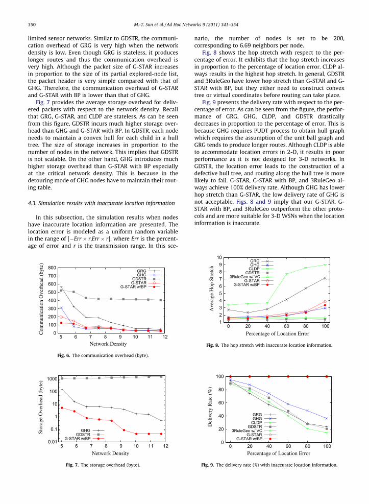
limited sensor networks. Similar to GDSTR, the communi-cation overhead of GRG is very high when the networkdensity is low. Even though GRG is stateless, it produceslonger routes and thus the communication overhead isvery high. Although the packet size of G-STAR increasesin proportion to the size of its partial explored-node list,the packet header is very simple compared with that ofGHG. Therefore, the communication overhead of G-STARand G-STAR with BP is lower than that of GHG.

Fig. 7 provides the average storage overhead for deliv-ered packets with respect to the network density. Recallthat GRG, G-STAR, and CLDP are stateless. As can be seenfrom this figure, GDSTR incurs much higher storage over-head than GHG and G-STAR with BP. In GDSTR, each nodeneeds to maintain a convex hull for each child in a hulltree. The size of storage increases in proportion to thenumber of nodes in the network. This implies that GDSTRis not scalable. On the other hand, GHG introduces muchhigher storage overhead than G-STAR with BP especiallyat the critical network density. This is because in thedetouring mode of GHG nodes have to maintain their rout-ing table.

4.3. Simulation results with inaccurate location information

In this subsection, the simulation results when nodeshave inaccurate location information are presented. Thelocation error is modeled as a uniform random variablein the range of [�Err � r,Err � r], where Err is the percent-age of error and r is the transmission range. In this sce-

0

100

200

300

400

500

600

700

800

5 6 7 8 9 10 11 12

Com

mun

icat

ion

Ove

rhea

d (b

yte)

Network Density

GRGGHG

GDSTRG-STAR

G-STAR w/BP

Fig. 6. The communication overhead (byte).

0.01

0.1

1

10

100

1000

5 6 7 8 9 10 11 12

Stor

age

Ove

rhea

d (b

yte)

Network Density

GHGGDSTR

G-STAR w/BP

Fig. 7. The storage overhead (byte).

nario, the number of nodes is set to be 200,corresponding to 6.69 neighbors per node.

Fig. 8 shows the hop stretch with respect to the per-centage of error. It exhibits that the hop stretch increasesin proportion to the percentage of location error. CLDP al-ways results in the highest hop stretch. In general, GDSTRand 3RuleGeo have lower hop stretch than G-STAR and G-STAR with BP, but they either need to construct convextree or virtual coordinates before routing can take place.

Fig. 9 presents the delivery rate with respect to the per-centage of error. As can be seen from the figure, the perfor-mance of GRG, GHG, CLDP, and GDSTR drasticallydecreases in proportion to the percentage of error. This isbecause GHG requires PUDT process to obtain hull graphwhich requires the assumption of the unit ball graph andGRG tends to produce longer routes. Although CLDP is ableto accommodate location errors in 2-D, it results in poorperformance as it is not designed for 3-D networks. InGDSTR, the location error leads to the construction of adefective hull tree, and routing along the hull tree is morelikely to fail. G-STAR, G-STAR with BP, and 3RuleGeo al-ways achieve 100% delivery rate. Although GHG has lowerhop stretch than G-STAR, the low delivery rate of GHG isnot acceptable. Figs. 8 and 9 imply that our G-STAR, G-STAR with BP, and 3RuleGeo outperform the other proto-cols and are more suitable for 3-D WSNs when the locationinformation is inaccurate.

1 2 3 4 5 6 7 8 9

10

0 20 40 60 80 100

Ave

rage

Hop

Str

etch

Percentage of Location Error

GRGGHG

CLDPGDSTR

3RuleGeo w/ VCG-STAR

G-STAR w/BP

Fig. 8. The hop stretch with inaccurate location information.

0

20

40

60

80

100

0 20 40 60 80 100

Del

iver

y R

ate

(%)

Percentage of Location Error

GRGGHG

CLDPGDSTR

3RuleGeo w/ VCG-STAR

G-STAR w/BP

Fig. 9. The delivery rate (%) with inaccurate location information.

1

1.5

2

2.5

3

0 10 20 30 40 50

Ave

rage

Hop

Str

etch

% of Nodes w/o Location Information

G-STARG-STAR w/BP

3RuleGeo

Fig. 12. The hop strecth with partial location information (10 iterations ofcentroid transformation).

M.-T. Sun et al. / Ad Hoc Networks 9 (2011) 341–354 351

4.4. Simulation results with partial location information

In this subsection, we demonstrate the simulation re-sults when some nodes in the network do not possessany location information. The percentage of nodes withoutlocation information ranges from 0% to 50%. In this sce-nario, the number of nodes is set to be 200, correspondingto 6.69 neighbors per node. The routing of GRG is nearlyrandom when some nodes do not have location informa-tion. In addition, PUDT in GHG, the right hand rule usedin CLDP to remove cross edges, and the construction of ahull tree in GDSTR all assume that nodes have locationinformation. The only protocols that work in locationlessnetwork are our two G-STAR variations and 3RuleGeo withvirtual coordinates. Therefore, in this scenario we compareonly the performance of G-STAR, G-STAR with BP, and3RuleGeo. For fair comparison, all three protocols makeuse of virtual coordinates, which are computed by centroidtransformation [15].

Figs. 10–12 demonstrate the hop stretch with respect tothe percentage of nodes without location information for 0,1, and 10 iterations of centroid transformation. As shownin the figure, the hop stretch increases when more numberof nodes do not hold location information. In addition,higher number of iterations of centroid transformationleads to smaller hop stretch. Among the tree protocols,we can see that BP is very effective in reducing the hop

1 2 3 4 5 6 7 8 9

10

0 10 20 30 40 50

Ave

rage

Hop

Str

etch

% of Nodes w/o Location Information

G-STARG-STAR w/BP

3RuleGeo

Fig. 10. The hop stretch with partial location information (0 iteration ofcentroid transformation).

1

2

3

4

5

6

0 10 20 30 40 50

Ave

rage

Hop

Str

etch

% of Nodes w/o Location Information

G-STARG-STAR w/BP

3RuleGeo

Fig. 11. The hop stretch with partial location information (1 iteration ofcentroid transformation).

stretch in case location information of some nodes is notavailable.

Figs. 13–15 show that the communication overheadwith respect to the percentage of nodes without locationinformation for 0, 1, and 10 iterations of centroid transfor-mation. As can be seen, the communication overhead de-creases as the number of iteration increases. Comparedwith 3RuleGeo, G-STAR incursless communication over-head. This is because that G-STAR does not record the same

0

10000

20000

30000

40000

50000

0 10 20 30 40 50

Com

mun

icat

ion

Ove

rhea

d (b

yte)

% of Nodes w/o Location Information

G-STARG-STAR w/BP

3RuleGeo

Fig. 13. The communication overhead with information (0 iteration ofcentroid transformation).

0

2000

4000

6000

8000

10000

12000

14000

0 10 20 30 40 50

Com

mun

icat

ion

Ove

rhea

d (b

yte)

% of Nodes w/o Location Information

G-STARG-STAR w/BP

3RuleGeo

Fig. 14. The communication overhead with partial location information(1 iteration of centroid transformation).

0

2000

4000

6000

8000

10000

12000

14000

0 10 20 30 40 50

Com

mun

icat

ion

Ove

rhea

d (b

yte)

% of Nodes w/o Location Information

G-STARG-STAR w/BP

3RuleGeo

Fig. 15. The communication overhead with partial location information(10 iterations of centroid transformation).

0

20

40

60

80

100

5 6 7 8 9 10 11 12

Del

iver

y R

ate

(%)

Network Density

GRGGHG

CLDPGDSTRG-STAR

G-STAR w/BP

Fig. 16. The delivery rate (%) (SNR is 5 dB).

0

20

40

60

80

100

5 6 7 8 9 10 11 12

Del

iver

y R

ate

(%)

Network Density

GRGGHG

CLDPGDSTRG-STAR

G-STAR w/BP

Fig. 17. The delivery rate (%) (SNR is 20 dB).

352 M.-T. Sun et al. / Ad Hoc Networks 9 (2011) 341–354

node ID in the partial explored-node list. G-STAR wit BP re-quires the smallest amount of communication overheadamong three protocols.

4.4.1. Simulation results in wireless fading modelIn this subsection, we show the simulation results when

the Rayleigh fading channel model is applied. Figs. 16 and17 illustrate the delivery rate with respect to the networkdensity with the SNR being set to 5dB and 20dB, respec-tively. Generally, the lower value of SNR, the more a losswireless link experiences. As shown in the figures, all pro-tocols result in higher delivery rate when SNR is set to

20dB. G-STAR and G-STAR with BP achieve higher deliveryrate than the other protocols regardless of the dB value.This is because our metric considers the effect of wirelessfading and avoids links with higher error rate. In addition,unlike other protocols, G-STAR and G-STAR with BP do nothave the detouring mode. This means that our protocolscan always take the effect of wireless fading intoconsideration.

5. Conclusion

Routing in 3-D wireless sensor networks (WSNs) ischallenging due to their resource constraints and dynamicnature. While the stateless property of existing geometricrouting protocols is attractive, they are not appropriatefor 3-D WSNs because of their tendency to incur highercommunication and storage overheads as well as theirquick performance degradation when the location infor-mation of some nodes is inaccurate or missing. In this pa-per, we propose a stateless geometric routing protocol for3-D wireless sensor networks, namely Geometric STAtelessRouting (G-STAR). Our routing protocol builds a location-based tree on-the-fly and finds a short path when travers-ing the tree. G-STAR is robust in the sense that it functionswell even when the location information is inaccurate ornot available for some nodes in the network. To further re-duce the path length, we propose a light-weight algorithm,namely Branch Pruning, to effectively optimize the pathobtained from the proposed G-STAR routing protocol. Theextensive simulation results have validated that the pro-posed routing algorithms achieve much higher deliveryrate and competitive hop stretch compared with existing3-D routing protocols, including GRG, GHG, CLDP, GDSTR,and 3RuleGeo.

References

[1] E.M. Sozer, M. Stojanovic, J.G. Proakis, Underwater acousticnetworks, IEEE Journal of Oceanic Engineering 25 (1)2000 72–83.

[2] V.R. Syrotiuk, C.J. Colbourn, Routing in mobile aerial networks, in:Proceedings of WiOpt, 2003, pp. 293–301.

[3] I.F. Akyildiz, W. Su, Y. Sankarasubramaniam, E. Cayirci, Wirelesssensor networks: a survey, Computer Networks 382002 393–422.

[4] C.E. Perkins, P. Bhagwat, Highly dynamic destination-sequenceddistance-vector routing (DSDV) for mobile computers, in:Proceedings of the ACM International Conference onCommunications Architectures, Protocols and Appliations(SIGCOMM), 1994, pp. 234–244.

[5] D.B. Johnson, Routing in ad hoc networks of mobile hosts, in:Proceedings of IEEE Internatinal Workshop on Mobile ComputingSystems and Applications, 1994, pp. 158–163.

[6] P. Bose, P. Morin, I. Stojmenovic, J. Urrutia, Routing with guaranteeddelivery in ad hoc wireless networks, in: Proceedings of the 3rdInternational Workshop on Discrete Algorithms and Methods forMobile Computing and Communications (DIAL-M), 1999, pp. 48–55.

[7] B. Karp, H.T. Kung, GPSR: greedy perimeter stateless routing forwireless networks, in: Proceedings of the ACM InternationalConference on Mobile Computing and Networking (MOBICOM),2000, pp. 243–254.

[8] F. Kuhn, R. Wattenhofer, Y. Zhang, A. Zollinger, Geometric ad-hocrouting: of theory and practice, in: Proceedings of the 22nd AnnualSymposium on Principles of Distributed Computing (PODC), 2003.

[9] B. Leong, B. Liskov, R. Morris, Geographic routing withoutplanarization, in: Proceedings of the 3rd Conference on NetworkedSystems Design and Implementation (NSDI), 2006, pp. 25–25.

[10] Y.-J. Kim, R. Govindan, B. Karp, S. Shenker, Geographic routing madepractical, in: Proceedings of the USENIX Symposium on NetworkedSystems Design and Implementation (NSDI), 2005, pp. 217–230.

M.-T. Sun et al. / Ad Hoc Networks 9 (2011) 341–354 353

[11] R. Kleinberg, Geographic routing using hyperbolic space, in:Proceedings of the IEEE International Conference on ComputerCommunications (INFOCOM), 2007, pp. 1902–1909.

[12] R. Flury, R. Wattenhofer, Randomized 3D geographic routing, in:Proceedings of the IEEE International Conference on ComputerCommunications (INFOCOM), 2008, pp. 834–842.

[13] C. Liu, J. Wu, Efficient geometric routing in three dimensional ad hocnetworks, in: Proceedings of the IEEE International Conference onComputer Communications (INFOCOM), Mini Conference, 2009.

[14] A. Rao, S. Ratnasamy, C. Papadimitriou, S. Shenker, I. Stoica,Geographic routing without location information, in: Proceedingsof the 9th Annual International Conference on Mobile Computingand Networking (MOBICOM), 2003, pp. 96–108.

[15] T. Watteyne, I. Augé-Blum, M. Dohler, S. Ubéda, D. Barthel, Centroidvirtual coordinates – a novel near-shortest path routing paradigm,Computer Network 53 (10) (2009) 1697–1711.

[16] T. Watteyne, D. Simplot-Ryl, I. Auge-Blum, M. Dohler, On usingvirtual coordinates for routing in the context of wireless sensornetworks, in: Proceeding of the International Symposium onPersonal, Indoor and Mobile Radio Communications (PIMRC), 2007.

[17] T. Watteyne, I. Auge-Blum, M. Dohler, D. Barthel, Geographicforwarding in wireless sensor networks with loose position-awareness, in: Proceeding of the International Symposium onPersonal, Indoor and Mobile Radio Communications (PIMRC), 2007.

[18] M. Caesar, M. Castro, E.B. Nightingale, Virtual ring routing: networkrouting inspired by DHTs, in: Proceedings of the ACM InternationalConference on Communications Architectures, Protocols andApplications (SIGCOMM), 2006, pp. 351–362.

[19] A. Awad, C. Sommer, R. German, F. Dressler, Virtual cord protocol(vcp): a flexible dht-like routing service for sensor networks, in:Proceedings of the IEEE International Conference on Mobile Ad-hocand Sensor Systems (MASS 2008), 2008, pp. 133–142.

[20] I. Stojmenovic, M. Russell, B. Vukojevic, Depth first search andlocation based localized routing and QoS routing in wirelessnetworks, in: Proceedings of the International Conference onParallel Processing (ICPP), 2000, p. 173.

[21] I. Stojmenovic, M. Russell, B. Vukojevic, Depth first search andlocation based localized routing and QoS routing in wirelessnetworks in: Proceedings of the International Conference onParallel Processing (ICPP), 2002, pp. 149–165.

[22] F. Kuhn, R. Wattenhofer, A. Zollinger, Asymptotically optimalgeometric mobile ad-hoc routing, in: Proceedings of the 6thInternational Workshop on Discrete Algorithms and Methods forMobile Computing and Communications (DIALM), 2002.

[23] F. Kuhn, R. Wattenhofer, A. Zollinger, Worst-case optimal andaverage-case efficient geometric ad-hoc routing, in: Proceedings ofthe ACM International Symposium on Mobile Ad Hoc Networkingand Computing (MobiHoc), 2003, pp. 267–278.

[24] K. Garbriel, R. Sokal, A new statistical approach to geographicvariation analysis, Systematic Zoology 18 (1969) 259–278.

[25] G. Toussaint, The relative neighborhood graph of a finite planarset,Pattern Recognition 12 (4) (1980) 261–268.

[26] X.-Y. Li, G. Calinescu, P.-J. Wan, Y. Wang, Localized delaunay triangu-lation with application in ad hoc wireless networks, IEEETransactions on Parallel Distributed Systems 14 (10) (2003) 1035–1047.

[27] H. Yan, Z.J. Shi, J.-H. Cui, DBR: depth-based routing for underwatersensor networks, in: Proceedings of the IFIP Networking, 2008, pp.1–13.

[28] D. Pompili, T. Melodia, I.F. Akyildiz, Routing algorithms for delay-insensitive and delay-sensitive applications in underwater sensornetworks, in: Proceedings of the ACM/IEEE International Conferenceon Mobile Computing and Networking (MOBICOM), 2006.

[29] N. Nicolaou, A. See, P. Xie, J.-H. Cui, D. Maggiorini, Improving therobustness of location-based routing for underwater sensornetworks in: Proceedings of the IEEE OCEANS, 2007, pp. 18–21.

[30] J.F. Kurose, K.W. Ross, Computer Networking: A Top-DownApproach, fifth ed.2009, Addison-Wesley Publishing Company, 2009.

[31] R. Ramanathan, R. Hain, Topology control of multihop wirelessnetworks using transmit power adjustment, in: Proceedings of theIEEE 23rd International Conference on Computer Communication(INFOCOM), 2000, pp. 404–413.

[32] M. Bahramgiri, M. Hajiaghayi, V.S. Mirrokni, Fault-tolerant and 3-dimensional distributed topology control algorithms in wirelessmulti-hop networks, Wireless Networks 12 (2) (2006) 179–188.

[33] A. Ghosh, Y. Wang, B. Krishnamachari, M. Hsieh, Efficient distributedtopology control in 3-dimensional wireless networks, in:Proceedings of the IEEE 4th International Conference on Sensor,Mesh and Ad Hoc Communications and Networks (SECON), vol. 12,2007, pp. 91–100.

[34] T.H. Cormen, C.E. Leiserson, R.L. Rivest, C. Stein, Introduction toAlgorithms, second ed.2001, The MIT Press, 2001.

[35] S. Even, Graph Algorithms1979, Computer Science Press, 1979.[36] B. Bollobas, Random Graphs1985, Academic Press, 1985.[37] X. Ma, M.-T. Sun, X. Liu, G. Zhao, An efficient path pruning algorithm

for geographical routing in wireless networks, IEEE Transactions onVehicular Technology 57 (4) (2008) 2474–2488.

[38] T.S. Rappaport, Wireless Communications: Principles and Practice,second ed.2001, Princeton-Hall, 2001.

[39] K. Seada, M. Zuniga, A. Helmy, B. Krishnamachari, Energy-efficientforwarding strategies for geographic routing in lossy wireless sensornetworks, in: Proceedings of the 2nd International Conference onEmbedded Networked Sensor Systems (SenSys), 2004, pp. 108–121.

[40] B.R. Hamilton, X. Ma, Noncooperative routing with cooperativediversity, in: Proceedings of the IEEE International Conference onCommunications (ICC), 2007, pp. 4237–4242.

[41] The Network Simulator (ns-2), <http://www.isi.edu/nsnam/ns/>.[42] IEEE 802.11b Standard, <http://standards.ieee.org/getieee802/

download/802.11b-1999.pdf>.

Min-Te Sun received his B.S. degree inMathematics from National Taiwan Univer-sity in 1991, the M.S. degree in ComputerScience from Indiana University in 1995, andthe Ph.D. degree in Computer and InformationScience from the Ohio State University in2002. Since 2008, he has been with Depart-ment of Computer Science and InformationEngineering at National Central University,Taiwan. His research interests include dis-tributed algorithm design and wireless net-work protocol development.

Kazuya Sakai received his B.S. and M.S.degree from Kansai University, Osaka, Japan,in 2004 and 2007, both in Electronics Engi-neering. Since 2008, he has been a graduatestudent of Department of Computer Scienceand Software Engineering at Auburn Univer-sity. His research interests are in the area ofwireless networks and mobile computing,including distributed algorithms, routingprotocols, secure.

Benjamin Russell Hamilton received theB.S.E.E degree from Auburn University in 2005and the M.S.E.E degree from Georgia Instituteof Technology in 2007. Since 2007, he hasbeen pursuing the Ph.D. degree in ElectricalEngineering at Georgia Institute of Technol-ogy. He performed research on routing in ad-hoc and wireless sensor networks from 2006to 2009. He has interned at General DynamicsC4 Systems, where he conducted research onpeak-average power ratio and pilot design forOFDM systems. In 2009, he was awarded the

Georgia Tech Research Institute Shackleford Fellowship, and is currentlyresearching location estimation and tracking in ad-hoc networks.

354 M.-T. Sun et al. / Ad Hoc Networks 9 (2011) 341–354

Wei-Shinn Ku received the Ph.D. degree inComputer Science from the University ofSouthern California (USC) in 2007. He alsoobtained M.S. degrees in both Computer Sci-ence and Electrical Engineering from USC in2003 and 2006, respectively. He is a graduateof National Taiwan Normal University. He isnow an assistant professor with the Depart-ment of Computer Science and SoftwareEngineering at Auburn University. Hisresearch interests include spatial and tempo-ral data management, mobile data manage-

ment, geographic information systems, and security and privacy.

Xiaoli Ma received the B.S. degree in Auto-matic Control from Tsinghua University, Bei-jing, China in 1998, the M.S. degree inElectrical Engineering from the University ofVirginia in 2000, and the Ph.D. degree inElectrical Engineering from the University ofMinnesota in 2003. After receiving her Ph.D.,she joined the Department of Electrical andComputer Engineering at Auburn University,where she was an assistant professor untilDecember 2005. Since January 2006, she hasbeen an assistant professor with the School of

Electrical and Computer Engineering at Georgia Tech. Her researchfocuses on signal processing for communications and networking,

including transceiver designs for wireless time- and frequency-selectivechannels, channel estimation and equalization, carrier frequency syn-chronization for OFDM systems, acoustic echo cancellation, networkperformance analysis, and cooperative designs for wireless networks.Ma is a member of the Signal Processing Theory and Methods (SPTM) andSignal Processing for Communications and Networking (SPCOM) Tech-nical Committees of the IEEE Signal Processing Society. She was awardedthe Lockheed Martin Aeronautics Company Dean’s Award for TeachingExcellence by College of Engineering at Georgia Tech in 2009.