VOLUME I PERFORMANCE FLIGHT TEST PHASE

CHAPTER 9 ENERGY

^

>£>*

AUGUST 1991 USAF TEST PILOT SCHOOL

EDWARDS AFB, CA

I Approved for public rate-erne; ! Distribution Uni;: r<cA

19970116 079

Table of Contents

9.1 INTRODUCTION 9.1 9.1.1 AIRCRAFT PERFORMANCE MODELS 9.1 9.1.2 NEED FOR NONSTEADY STATE MODELS 9.1

9.2 STEADY STATE CLIMBS AND DESCENTS 9.2 9.2.1 FORCES ACTING ON AN AIRCRAFT IN FLIGHT 9.2 9.2.2 ANGLE OF CLIMB PERFORMANCE 9.5 9.2.3 RATE OF CLIMB PERFORMANCE 9.9 9.2.4 TIME TO CLIMB DETERMINATION 9.14 9.2.5 GLIDING PERFORMANCE 9.16 9.2.6 POLAR DIAGRAMS 9.18

9.3 BASIC ENERGY STATE CONCEPTS 9.22 9.3.1 ASSUMPTIONS 9.22 9.3.2 ENERGY DEFINITIONS 9.23 9.3.3 SPECD7IC ENERGY 9.24 9.3.4 SPECD7IC EXCESS POWER 9.24

9.4 THEORETICAL BASIS FOR ENERGY OPTIMIZATIONS 9.25

9.5 GRAPHICAL TOOLS FOR ENERGY APPROXIMATION 9.25 9.5.1 SPECD7IC ENERGY OVERLAY 9.26 9.5.2 SPECmC EXCESS POWER PLOTS 9.28

9.6 TIME OPTIMAL CLIMBS 9.36 9.6.1 GRAPHICAL APPROXIMATIONS TO RUTOWSKI

CONDITIONS 9.36 9.6.2 MINIMUM TIME TO ENERGY LEVEL PROFILES 9.37 9.6.3 SUBSONIC TO SUPERSONIC TRANSITIONS 9.38

9.7 FUEL OPTIMAL CLIMBS 9.40 9.7.1 FUEL EFFICIENCY 9.41 9.7.2 COMPARISON OF FUEL OPTIMAL AND TIME OPTIMAL

PATHS 9.43

9.8 MANEUVERABILITY 9.44

9.9 INSTANTANEOUS MANEUVERABILITY 9.44 9.9.1 LIFT BOUNDARY LIMITATION 9.45 9.9.2 STRUCTURAL LIMITATION 9.46 9.9.3 qLIMTTATION 9.46 9.9.4 PILOT LIMITATIONS 9.46

9.10 THRUST LIMITATIONS/SUSTAINED MANEUVERABILITY 9.47 9.10.1 SUSTAINED TURN PERFORMANCE 9.47

9.10.2 FORCES IN ATURN 9.47

9.11 VERTICAL TURNS 9-52

9.12 OBLIQUE PLANE MANEUVERING 9.53

9.13 TURNING PERFORMANCE CHARTS 9.55

9.14 THRUST LIMITED VERSUS LIFT LIMITED TURNS 9.62

9.15 SUSTAINED TURN PERFORMANCE FROM LEVEL ACCELERATION 9-63

9.16 DYNAMIC PERFORMANCE TESTING 9.71 9.16.1 INTRODUCTION • 9.71 9.16.2 MEASUREMENT TECHNIQUES 9.75 9 16.3 CORRECTION AND TRANSFORMATIONS 9.77 9.16.4 CONCLUSION 9.80

9 17 DATA COLLECTION FOR ENERGY METHODS 9.80 9 17.1 INTERNAL MEASUREMENT TECHNIQUES 9.80

9.17.1.1 PRESSURE METHODS 9.80 9.17.1.2 ACCELERATION MEASUREMENTS 9.80

9.17.2 EXTERNAL MEASUREMENT METHODS 9.81 9.17.2.1 RADAR TRACKING 9.81 9.17.2.2 OPTICAL TRACKING (OT) 9.81 9.17.2.3 LASER TRACKING (LT) 9.81

9.17.3 MODERN METHODS 9.81 9.17.4 RELATIVE MERITS 9.82

9.18 CLIMB AND DESCENT TESTS 9.82 9.18.1 SAWTOOTH CLIMB TEST 9.83 9.18.2 LEVEL FLIGHT ACCELERATION TEST 9.84

9.18.2.1 METHOD 9.85 9.18.2.2 PREFLIGHT PREPARATION 9.85 9.18.2.3 USES 9.86 9.18.2.4 LIMITATIONS 9.86

9183 CHECK CLIMB TEST FOR JET AHtCRAFT 9.86 9.18.3.1 PREFLIGHT PREPARATION 9.87 9.18.3.2 FLIGHT TECHNIQUES 9.87

9 184 RECD?ROCATING ENGINE CHECK CLIMB TEST 9.89 9.18.4 TURBOPROP ENGINE CHECK CLIMB TEST 9.89

9.19 TURNING PERFORMANCE TESTS 9.89 9 19.1 STABILIZED TURN METHOD 9.89

9.19.1.1 STABLE g METHOD 9.90 9 19.1.2 CONSTANT AD3SPEED METHOD 9.90

9.19.1.2.1 TIMED TURN TECHNIQUE 9.91

ii

9.20 DYNAMIC PERFORMANCE METHODS 9.91 9.20.1 PUSH OVER - PULL UP (POPU) 9-91 9.20.2 WIND UP TURN (WUT) 9.92 9.20.3 SPLIT-S (SS) 9.92

9.21 SAMPLE DATA CARDS 9.92

9.22 SUMMARY 9.94

in

9.1 INTRODUCTION To evaluate modern aircraft and aircraft systems requires an understanding of how

aerodynamic performance can be optimized. Performance specifications today go well beyond

point design specifications and depend heavily on optimization to fit specific tactical

requirements whether the vehicle is designed as an interceptor, an air superiority fighter, a strategic airlifter, a strategic bomber, or for any other operational role. The goal is to demand a performance efficiency covering the entire flight envelope that will meet the operational need with the best overall combination of armament, engine, and airframe. The

F-14 and F-15 were the first generation of fighter aircraft to be designed and evaluated

within this approach. Newer fighter designs like the F-16, the F-18, the Tornado, and the

Mirage 2000 have been conceived with full cognizance of the need for optimized performance.

9.1.1 AIRCRAFT PERFORMANCE MODELS The almost universally accepted mathematical model for aircraft performance is a point-mass model; that is, we need only consider the forces acting on the center of gravity of the airplane. But even this simple set of governing equations can be manipulated under a wide range of

assumptions. Bryson, Desai, and Hoffman (10.1:481ff) have conveniently catalogued several

of these approximations from an optimal control perspective. For our convenience, we will lump these models into three categories:

1. Steady state approximation 2. Energy state approximation 3. Higher order optimal control approximations

In this chapter, we will consider all three of these models. However, due to the complexity of higher order optimal control approximations we will limit ourselves to a conceptual approach.

9.1.2 NEED FOR NONSTEADY STATE MODELS The classical approach to aircraft performance problems is a "static" or steady state one. For this approximation, either true airspeed or altitude (or both) must be held constant. Therefore, the model is inadequate for analyzing climb profiles, for example, of supersonic aircraft. Both true airspeed and altitude change rapidly for such airplanes. Obviously, the steady state approximation cannot cope satisfactorily with vehicles like the Space Shuttle Orbiter which never achieves steady state flight.

9.1

9.2 STEADY STATE CLIMBS AND DESCENTS Climbs and descents at constant true airspeed (dV/dt. 0) are a subset of problems associated with performance optimization. They could be called "static" performance problems and, as

such, are useful as first order tools of analysis. For our purposes, they also serve as an

introduction to the energy state approximation.

9.21 FORCES ACTING ON AN AIRCRAFT IN FLIGHT The forces acting on an aircraft in flight are conveniently resolved perpendicular and parallel

to the direction of flight, as shown in Figure 9.1.

FIGURE 9.1 FORCES ACTING ON AN AIRCRAFT IN FLIGHT (ZERO

BANK ANGLE)

Perpendicular to the flight path

L - Wcos Y * F« sin <a * a** * ma*

Where a is the angle of attack, c^ is the thrust angle of incidence or the angular difference between the thrust line and tixe fuselage reference line (FRL), and a, is the acceleration

perpendicular to the flight path.

9.2

Parallel to the flight path f

F.cos (a + (Xj.) - D - W sin y « ma X

With the following relatively minor simplifying assumptions

a « 0, ar - 0, ax - 0,

that is angle of attack is small and the engines are closely aligned with the fuselage reference

line

dV and recalling ax = —_

these equations take on simpler, more recognizable forms.

L - W cos Y " °

(9.1)

Fn - D - W sin Y - ~g£

(9.2)

For purposes of yrpwnwfag how to maximize y (since we are analyzing climb performance), true airspeed is held constant. At a constant true airspeed, dV/dt = 0. With this restriction,

Equation 9.2 becomes

F„ - D = W sin Y

which gives a useful expression for gamma

9.3

y = sin" w (9.3)

Where " ~ is specific excess thrust, "specific" because we are examining the excess W

thrust at that specific weight By maximising specific thrust, we will maximize the climb

angle, y.

Now, multiplying by V on both sides gives

V sin y = ^} But V sin y is simply the rate of climb or rate of descent, as Figure 9.2 illustrates.

FIGURE 9.2 RATE OF CLIMB

(9.4)

9.4

This expression clearly shows that if net thrust is greater than drag, dh/dt is positive; that is F > D produces a climb. Conversely, Fn < D produces a descent and dh/dt is negative.

Gliding flight is he special case when Fn = 0. This simple expression also allows the careful student to deduce the effects of altitude, weight, wind, and velocity on angle of chmb

performance and rate of climb performance.

9.2.2 ANGLE OF CLIMB PERFORMANCE As Equation 9.3 clearly shows, the flight path (or climb) angle y depends on specific excess

thrust: (F -D)/W. As an aircraft with an air breathing powerplant climbs, the propulsive thrust decreases as altitude increases. Drag remains essentially constant. Thus, there is an

absolute ceiling where Fn = D and y = 0. In other words, increasing altitude decreases

specific excess thrust and the climb angle.

The effect of increasing weight on angle of climb is also obvious from Equation 9.3.

Increasing weight directly reduces the climb angle because of the reciprocal relationship.

A steady wind actually has no effect on the angle of climb of an aircraft within a moving air mass However, the prime reason for optimizing angle of climb (or descent) is to gam

obstacle clearance during either the takeoff or landing phases of flight. The maximum climb angle must give the most altitude gained for horizontal distance covered. Winds do affect

this horizontal distance and give apparent changes in y as depicted in Figure 9.3. Not surprisingly, the obvious point is to always land and takeoff into a headwind if obstacle

clearance is a concern.

FIGURE 9.3 WIND EFFECT ON CLIMB ANGLE

9.5

Thrust curves show that excess thrust, Fn - D is a function of airspeed. Figure 9.4 illustrates this point for the T-38. Whatever the type of propulsion - jet, turboprop, or reciprocating engine - the aircraft must be flown at the velocity where ""»^"^ «"»"« thrust occurs to

achieve the maximum climb angle.

Typically, the net thrust available from a pure turbojet varies little with airspeed at a given altitude. The J-85 operated at military thrust in the T-38, as shown in Figure 9.4a illustrates this characteristic well For a turbofan, that is sometimes true. Figure 9.4b shows the F100- 220 at military thrust in the F-15C. Therefore, a jet aircraft, lacking any form of thrust augmentation, usually climbs at the velocity for minimum drag (or minimum thrust required) to achieve the maximum angle of climb. This classical result leads to the sometimes

overemphasized notion that y^ occurs at YLT^-

8 1 1 WT 10,000 LBS STANDARD DAY

l-CLEAN —

100 200 300 400 500 600

TRUE AIRSPEED (KTS)

FIGURE 9.4a T-38 THRUST AND DRAG

9.6

P -ISC

SPLtD -POWtR MRP

CONK ICUKH1 ION '4 i Bin-n i 4 i nm .«« r lou fw «;<?u nit 1 roHT P0HI.K

KTRS „ im *uti JMt 414* «IIU Mit) »l*U

«LT -0. GlEVtl -- 1 .00

*

- u

"~o. ■ <n

to OOo

Thrust Available ...

45000/—Tl

tUOOOf^ll o cr £° Oo

o

3JOOO#-4II

z o o

= N~ ■¥ .00 0.^0 0.«0 0.R0 O.aU 1 Ü0 1

nHCH NUMH1.R <ro

FIGURE 9.4b F-15C THRUST AND DRAG

This generalization is based on too many assumptions to be absolutely accurate. Any variation in thrust available with airspeed obviously affects the optimum velocity for maximum climb angle. Careful examination of Figure 9.4 reveals that in the T-38 any true airspeed between 240 and 270 knots results in approximately the same specific excess thrust, hence about the same y. Any large variation in thrust available with airspeed, as is illustrated in the maximum afterburner curve for the T-38, clearly destroys the idea that yBSI

always occurs Vj^p

9.7

The point is that precise determination of maximum angle of climb performance depends on specific excess thrust, which in turn requires knowledge of both airframe drag characteristics and propulsive system characteristics. The rule of thumb that a jet aircraft should climb at VT,n for obstacle clearance can be grossly in error for thrust augmentation, turboprops, or JgtaTdnnfk Figure 9.4a presents the T-38 afterburner thrust curve. Notice the characteristic shape of this curve. Depending on engine design, the maximum excess thrust in afterburner may occur at a point higher than V^ or minimum drag. In the case of a turboprop aircraft, the thrust tends to decrease with an increase in velocity as shown m

Figure 9.5, a comparison of turboprop and turbojet thrust with speed. If a drag curve were superimposed on this figure, it could be seen that the maximum value of excess thrust nught

occur at a speed less than V^^. Again, this would depend on the exact shape of the

turboprop thrust curve.

FIGURE 9.5 THRUST VARIATIONS WITH SPEED

Finally, a propeller driven aircraft must account for propeller efficiencies and has its own

9.8

peculiar thrust available curve. Figure 9.6 shows a typical piston aircraft thrust and drag

curve. Note the location of maximum excess thrust.

FIGURE 9.6 PISTON AIRCRAFT THRUST/DRAG CURVES

But, whether specific excess thrust is measured directly or calculated from independent estimates of thrust, drag, and weight, this parameter determines angle of climb performance.

9.2.3 RATE OF CLIMB PERFORMANCE Referring again to Equation 9.4, rate of climb, dh/dt, depends upon specific excess power. The terminology is analogous to specific excess thrust, which was defined as the difference between net thrust available and drag (or thrust required) at a specific weight. Excess power is similarly defined as the difference between the power available to do work in a unit of time

and the work done by drag per unit of time.

9.9

F V s power available

DV m power dissipated by drag {or power required)

dh (F„ - P) V m FnV- DV _ PA~Pr

St " w w w

(9.5)

Figure 9.7 shows typical P. and Pr curves for a turbojet, turboprop, and piston engined aircraft. Note the shape of the Pr curve. It is formed by multiplying true airspeed (V) by the drag value at that speed. Similarly, the P. curve was derived by multiplying V by the thrust at that speed. For the military power turbojet, the thrust was generalized to be flat across the airspeed spectrum. This is known as a "flat rated" engine. As the airspeed scale is linear, the result is a straight line originating at the origin, where V = 0. The slope of the curve is directly proportional to the magnitude of thrust. For the turboprop and piston aircraft, thrust was not constant with speed. Therefore, the slope of the curve for P. changes

as the aircraft's true airspeed changes.

9.10

Reqd

Power

Power

Power

Available

Available

FIGURE 9.7 P. AND Pr CURVES (VARIOUS POWERPLANTS)

9.11

Altitude has an effect on rate of climb similar to its effect upon angle of climb. Rate of climb at the absolute ceiling goes to zero because Fn = D and, obviously, excess power is nil. In military specifications, there are two other performance ceilings defined by rate of climb performance. The service ceiling and combat ceiling are respectively the altitudes where 100 ff min and 500 ft/min rates of climb can be maintained.

Weight affects rate of climb directly and in the same manner as it does climb angle. Increasing weight with no change in excess power reduces rate of climb.

Wind affects rate of climb negligibly unless gradient and direction changes are large within

the air mass.

True airspeed strongly affects rate of climb performance since thrust and drag are functions of velocity themselves, and further specific excess power explicitly depends upon true airspeed according to Equation 9.4. Figure 9.8 illustrates the typical power available and power required for a turbojet and propeller aircraft. The propeller driven aircraft obtains maximum rate of climb at a true airspeed close to the velocity for maximum L J). For jet aircraft, maximum rate of climb occurs at some higher true airspeed. Figure 9.9 compares the power required and power available (both at military and maximum power) for the T-38. This chart is based on Figure 9.4a. Based upon your knowledge of how P, curves are derived, it should be obvious why the maximum (afterburner) power curve is shaped the way it is and what effect that may have on the true airspeed for maximum excess power.

9.12

cc tu

o 0.

1 1 I PROPAND JET

-AT SAME WEIGHT. A 7 ?0> <?

/- /

/ / 5

/ A

/MAX /!

/' 4

R/<

' R; JE '

c / r

LX /

> /

^

^ 1 1 TRUE AIRSPEED

FIGURE 9.8 TYPICAL RATE OF CLIMB PERFORMANCE

9.13

DC W «S o Q. ÜJ W EC o Z

WT 10,000 LBS STANDARD DAY 1

f

CLE AN 1 1 8

/ / r Si

/ f / 'I 6

1 f ■/

/

/ / 4

/ / 1 4

//

t

/ z '"7 /

/

/

200 400 600

TRUE AIRSPEED (FPS)

FIGURE 9.9 T-38 RATE OF CLIMB PERFORMANCE

9.2.4 TIME TO CLIMB DETERMINATION The climb performance parameter of most interest to the operational pilot is usually time required to climb to a given altitude. Rates of climb discussed so far are instantaneous values. At each altitude, there is one velocity which yields maximum rate of climb. That value of maximum rate of climb pertains only to that discrete altitude. Continuous variations

9.14

in rate of climb suggest a summation through integration (see Figure 9.10)

dt " OT ""els -i " fW

or

} * -1- J dh dh/dt

(9.6)

However, dh/dt is usually not available as an analytical function of altitude; hence, Equation

9.6 can rarely be integrated, except with graphical or numerical techniques.

FIGURE 9.10 TIME TO CLIMB

9.15

9.2.5 GLIDING PERFORMANCE Gliding flight (Fn = 0) offers a simple application of Equations 9.3 and 9.4. This special case also leads to results that further illuminate the usefulness and importance of the velocity for

maximum L/D. Attacking the angle of descent (negative angle of climb) problem first, the

ratio of the horizontal distance covered to altitude lost defines y. As can be seen from Figure

9.11.

or

L - N cos y

D « W sin Y

Z. = cot Y

(9.7)

FIGURE 9.11 FORCES ACTING IN A GLIDE

9.16

Equation 9.7 expresses the fact that when | y | is a minimum, | cot y | is a maximum.

In other words, when L/D is maximum, the maximum horizontal distance is achieved for a given altitude loss. The trigonometric relations show that the ratio of horizontal distance traveled to vertical distance (or horizontal velocity to vertical velocity for a constant true airspeed descent) is equal to L/D. Hence, L/D^ gives the "best" glide ratio and is frequently

called the glide ratio.

To minimize the rate of descent in a glide, Equation 9.4 is specialized with Fn = 0.

dh _ _DV

(9.8)

Once again, dh/dt is a function of "power" dissipated and is not a simple function of drag. If one assumes a parabolic drag polar, it can be shown that the velocity for minimum rate of descent is about 25% less than the true airspeed for niinimum glide angle. This result (which will be demonstrated in homework and class discussion) means that the pilot who tries to stretch his glide by minimizing sink rate is actually reducing the horizontal distance

covered (range) for a given loss in altitude.

Two identical sailplanes operating at different gross weights will have identical glide ratios, since they will have the same L/D ratio. Figure 9.12 illustrates two sets of equilibrium

conditions. Note that Lj > Lx to support

9.17

FIGURE 9.12 EFFECT OF WEIGHT ON GLIDE RATIO

the increased weight. But to obtain L/D»«, the pilot holds the same angle of attack. Thus,

to TTHP"i*flin the force equilibrium, he must increase speed to increase Lj to Lj. As the heavier

sailplane flies faster, it also generates more drag. Hence, the heavier aircraft flies faster, arriving sooner and descending faster, but covers the same distance. This principle is the driving influence behind jettisonable water ballast for competition sailplanes, when one of

the goals is to cover a given closed course distance in TrriniTrmm time.

9.2.6 POLAR DIAGRAMS Polar riiflgrf»™»» are graphical means of summarizing aircraft steady state performance. Three

conditions are assumed for any one diagram. 1. Aircraft weight is constant

2. Altitude is constant 3. Throttle setting is constant

A change in any one of these constants calls for a new diagram to describe the new steady state. Figure 9.13 is a typical polar diagram for military thrust in a jet aircraft.

9.18

> >

o o _l tu > -I < o

cc UJ >

MAXIMUM RATE OF CLIMB

MAXIMUM LEVEL FLIGHT SPEED

INCREASING a

TERMINAL VELOCITY

FIGURE 9.13 MILITARY THRUST POLAR DIAGRÄM

This plot represent all the combinations of vertical and horizontal velocities that the airplane can attain in unaccelerated flight at a given altitude, throttle setting, and weight.

Point 1, for example, represents the maximum attainable level flight speed with these conditions. Point 2 represents a steady state climb at the flight path angle (y2) indicated. A line drawn from the origin to any point on the diagram represents vectoriallv the true airspeed for that flight condition. The angle of climb for any steady state pair of velocity components is the angle between the true "airspeed vector" and the horizontal velocity component (x-axis). Point 3, the im»"'"""' value for rate of climb, obviously provides a lower climb angle *hp™ Point 4. The fact that Vmax is greater than V„ is driven home, if one

R/C notes the magnitudes of the true airspeed vectors for Points 3 and 4. It is graphically clear

9.19

from a diagram like this, one can obtain ymlix and the VY by simply drawing a line from the origin tangent to the curve. Point 5 depicts the stalling speed- This example represents an aircraft that is capable of climbing at military thrust when it stalls. Point 6 represents the vertical velocity the airplane could attain if it were diving with y = 90° at military thrust. This speed, termed the terminal velocity, is often of academic interest only because many aircraft would break up before it could be attained. This point highlights the fact that polar diagrams show only aerodynamic (thrust and drag) information; structural limitations, control limitations, and other non-aerodynamic constraints are not usually noted. Finally, the polar diagram can also have angle of attack annotations. At Point 5, the angle of attack is a.; at Point 4, a is that for best angle of climb; and at Point 6, a is the angle of attack for

zero lift. Hence, a increases as one travels in a counterclockwise direction around the polar.

Since weight, altitude, and power setting are constant, a family of curves is necessary to describe the effect of these variables. However, since each of these variables affects performance in a similar way, qualitatively any one of these changes can be represented by shifting the curve itself up or down. The power-off polar diagram, Figure 9. 14, shows the differences in airspeed for (1) Tni™™™™ glide angle, (2) minimum rate of descent, and (3) 7»iniTn»TTi speed. The fallacy of trying to "stretch the glide" by flying slower is graphically

portrayed, since y,,^ occurs at Point 1, where the true airspeed vector is tangent to the polar.

MIL THRUST

H

PARTIAL THRUST OR ABSOLUTE CEILING OR HIGH GROSS WEIGHT

POWER OFF OR OVERWEIGHT

FIGURE 9.14 FAMILY OF POLAR DIAGRAMS

9.20

For glider aircraft, the airspeed at Point 1 is often referred to as the maximum L/D airspeed, as it will result in the greatest distance traveled for a given altitude above the ground. Point 2 is known as the minimum sink airspeed. Flying this speed will result in the greatest time aloft for given altitude to lose. What is the result of slowing from maximum LflD speed to minimum sink airspeed as it pertains to descent angle, 7? From the polar diagram, it is easy to see that y increases. Conceptually, it is difficult to imagine how decreasing the rate of descent increases the descent angle. The answer is in how the aircraft drag curve transforms

when changed to a Pr curve. Figure 9.15 demonstrates.

FIGURE 9.15 D AND Pr CURVE COMPARISON

9.21

Notice the relationship between the two curves. The velocity for minimum drag will be the

point at which y will be a minimum value, as

Y ■ sin"1]-lE|, assuming Fn ■ 0

However, note that at this velocity the value for Pr is higher than the minimum Pr value.

From the expression

Vv » Z£Tf assuming FB - 0

notice that Vv is a minimum where Pr (or -DV) is a minimum.

Hence, in order to ininimize the rate of descent the aircraft must be flown at the minimum Pr velocity. But, in going back up to the drag curve it can be seen that the drag for the nunimum Pr velocity has increased in comparison to the drag value at maximum L/D

(minimum drag). Therefore, the glide angle (y) will increase.

In summary, polar diagrams are handy for visualizing some of the basic concepts of steady state climb and descent performance. Important parameters, like ym„, Vw Vma^c, are graphically portrayed However, because of the constraints used in their construction and the consequent necessity to examine families of curves, polar diagrams are little used by operators. Soaring buffs do use them in constructing "speed-to-fly" charts that specify optimum transit speeds between thermal activity. Apart from such uses where the variables are limited by the nature of the vehicle, polar diagrams are largely useful only as a teaching

tool.

9.3 BASIC ENERGY STATE CONCEPTS A more general approach to aircraft performance was formulated by Rutowski in the early l^ffs. His analysis is based on "the balance that must exist between the potential and kinetic energy exchange of the aircraft, the energy dissipated against the drag, and the energy derived from the fuel" (9.2:187). The definitions and explanations which follow are based on and generally parallel Rutowski's original development, though portions have been

altered to clarify and amplify the concepts.

9.3.1 ASSUMPTIONS

9.22

There are usually four basic assumptions made for elementary energy state analyses:

1. Configuration is fixed 2. Weight is constant 3. Load factor is constant

4. Thrust lever is fixed The underlying reason for each of these assumptions is to reduce the complexity of the

mathematical problem. In fact, as we will see, these assumptions allow us to define an

energy state with only two variables—altitude and true airspeed. However, these

assumptions can be relaxed for specific purposes. Weight and load factor may be changed. In general, tf"« will be considered outside the scope of this course. Interest in these changes

should be directed toward Rutowski's paper.

In addition to these four basic assumptions, we will be rather cavalier in this introductory course with the interchange between different forms of energy. As a first order approximation, we will assume that airspeed and altitude can be exchanged instantaneously

with no energy dissipation. Such processes are of course, idealized ones and would exceed angle of attack and load factor limitations if you attempted such maneuvers. But to add such constraints complicates the energy state approximation and obscures too many concepts for

our purposes.

9.3.2 ENERGY DEFINITIONS The total energy of an aircraft is comprised of kinetic energy in the form of airspeed and

potential energy in the form of altitude.

E = PE ■+• KE

W V2

(9.9)

An aircraft in a climb is increasing potential energy either by the expenditure of chemical energy (by the powerplant) or by decreasing kinetic energy (trading airspeed for altitude).

Descents are also a change in potential energy which may or may not be accompanied by a change in kinetic energy. Constant true airspeed descents, for example, involve a decrease in potential energy (and therefore total energy) due to the work done by drag forces.

9.23

9.3.3 SPECIFIC ENERGY In analyzing climbs and accelerations for aircraft having different weights at the same altitude-airspeed combinations, energy per pound of aircraft weight or "specific energy" is more convenient than total energy. Equation 9.9 can be rearranged and E, defined as specific

energy.

*.. * -1. + *L * W IZg

(9.10)

Occasionally, E, is called "energy height" since it has units of length only. Physically, this

terminology suggest that "energy height" is the altitude the aircraft would attain if all its

kinetic energy could be converted with no loss to potential energy. Alternatively, if all the altitude were converted to kinetic energy, the corresponding true airspeed is the maximum

speed attainable with a given specific energy level

9.3.4 SPECIFIC EXCESS POWER Perhaps the most important parameter in the energy methodology is obtained by differentiating Equation 9.10 with respect to time.

dEM dh + V dv "dT ~dt ~g~3E

(9.11)

It is not necessary to assume db/dt and dV/dt are zero as was done for steady state performance analysis. However, from Equation 9.2

F„ - D - W sxn V = —_ " ' gat

Dividing through by W/V and transposing

(J?\, - D) V dV " ' v - V sin Y + _1 -Zl

But V sin Y = db/dt, therefore:

9.24

~3F w (9.12)

The term on the right side of Equation 9.12 is excess thrust multiplied by velocity and normalized for weight. Since thrust lames velocity is power, dE/dt may be defined as specific excess power. We will define a new symbol for this term, P.:

dB P s * * -ar

P, characterizes the engine-airframe capability to change energy levels at a given airspeed, altitude, and power setting.

9.4 THEORETICAL BASIS FOR ENERGY OPTIMIZATIONS Having defined terms and introduced the energy approach by reviewing steady state performance considerations, a theoretical foundation for applying energy techniques must be laid. The idea of applying powerful mathematical tools like the calculus of variations to aircraft performance was suggested by Graham (9.2:190) in Rutowski's original paper. Theoreticians are still adding to our store of knowledge in applying these tools. The calculus of variations is the branch of mathematics that provides the theoretic foundation for the graphical tools that will be used for energy approximations. In essence, it provides a means by which to determine a function, over a definite integral, that results in a maxima or minima. A true understanding of the calculus of variations would require more time than is available for this course. A firm understanding is not required to master the energy approximation.

9.5 GRAPHICAL TOOLS FOR ENERGY APPROXIMATION Solutions to even the basic calculus of variations problem are best left to optimal control specialists. However, a number of simple graphical approximations and tools provide useful information to designers and operational tacticians. Since the most reliable raw data to construct these graphical tools come from flight tests, it is imperative that the test pilot and test engineer/navigator have a working knowledge of them.

9.25

9.5.1 SPECIFIC ENERGY OVERLAY Having specified h and V as dependent variables, it is customary to utilize standard linearly scaled rectangular coordinates to depict energy states in terms of these two variables. However, since the energy approximation requires consideration of events that take place at levels of constant energy, a constant E. grid is commonly overlaid on the h, V axes. Figure

9.16 shows such an overlay.

FIGURE 9.16 SPECIFIC ENERGY OVERLAY

As Equation 9.10 suggest, these lines of constant E. are parabolic segments, with the altitude intercept (Point A) representing a body having only potential energy (V = 0). Point B, on the

other hand, represents a body having only kinetic energy (h = 0).

One of the limitations (or perhaps fallacies) of the energy approach is also apparent from Figure 9.16. Note that time (the independent variable) does not appear on the specific energy grid. In his original formulation, Rutowski assumed that an exchange of potential energy for kinetic along a constant energy path could be made instantaneously. Anyone who has ever

9.26

tried to trade airspeed for altitude recognizes this approximation as rather crude; such maneuvers quickly exceed the assumptions of small a and negligible normal acceleration. Much of the work done to build on Rutowski's concept has been aimed at optimal solutions relaxing this impracticality (9.4:93 and 9.5:315). This simplification means that an aircraft could ideally zoom or dive between points C and D or any other points along a constant E,

contour in zero time.

801

o X

S 40 Q D I-

1 — N V -v^ N, X

_ N. s \ —-^ V ^ w N^ N \ \

N \ \

^ \ \ * N . \ N \ 1 M \ \ 1 1.0

MACH

2.0

\ \

^ \ \ \ \ \

- N N

^ \ \ \ ^ ^ \ N ^ \ N ^

\ \ \ \ \ ,

40 80

29 (1,000 FT)

FIGURE 9.17 ALTERNATIVE SPECIFIC ENERGY OVERLAYS

In addition to the basic representation of E. on h, V diagrams, there are several alternative ways to display the same information. Two such alternatives are shown in Figure 9.17. The h, M plot is a common substitution of dependent variables (M for V) for supersonic aircraft in operationally oriented literature. Notice the "knee" in the E grid lines when they are plotted on the h, M axes. It will be left as an exercise for the reader to show why this

discontinuity in slope arises.

Sometimes, plotting specific potential energy versus specific kinetic energy (V^g) is useful in graphically obtaining the points of tangency (a procedure to be elaborated upon later). The form of the overlay should be suited to the user's purpose; in any case, the information is

9.27

essentially the same. These overlays of constant E, allow one to choose paths of constant E,

or paths of known change in E,.

9.5.2 SPECIFIC EXCESS POWER PLOTS The specific excess power plot is the basic graphical tool used to display total performance capability of an aircraft with the energy approach. In order to understand the significance of this plot, and how changes in certain variables affect it, a brief discussion on how to produce the plot is required. The simplest approach is to begin with an introduction into one

of the flight test techniques, the level acceleration.

The level acceleration is but one of the techniques by which P. values may be obtained. In theory, the pilot performs an acceleration of the aircraft at a fixed power setting (usually military or *w»fannm power), 1 g, and constant tapeline altitude. That is, altitude remains

constant. Hence, from Equation 9.11.

dE, _ dh + V dV ' * "3t" ~ ~3E g~3£

with altitude constant, _. = 0. So,

p = vdv e' -g~dt

Now, referring back to Figure 9.7, notice that there are two points where Pr = PA. And

equation 9.12 told us:

dt W

but

s = P. dt a

9.28

and

FaV-DV _ Pa-Px

W w

so

p s _5—£

(9.13)

At these two points, where PP = P„ P. = 0. At each velocity between these points, P. > Pr so P. is positive and therefore the aircraft will accelerate. Outside these velocities P. is negative

and therefore the aircraft will be unable to accelerate.

Consequently, if the aircraft is accelerated from a velocity just faster than the slow speed Pa

= Pr point it will eventually increase airspeed out to the high speed P. = Pr point and stabilize. A plot of true airspeed as a function of time is produced. Figure 9.18 depicts a

hypothetical data plot.

FIGURE 9.18 LEVEL ACCEL V vs t

9.29

From this plot, P, can be computed for the interval between Vx and V2 using the equation

p - X&L e~ ffdt

since the tapeline height was held constant. The values of AV and At, depicted on the plot,

will be used as the estimate for -~ . The average velocity (V«_), defined as at

1 2 , will be the actual data point of interest. Therefore, the P. value computed will 2

apply at that point and can be computed by substituting values into the equation. From a qualitative stand point, knowing Equation 9.12, it can be seen that the slope of the curve in Figure 9.18 represents the relative magnitude of excess thrust. This understanding is left

to the reader.

As the value for P. was determined for this point, so it is determined for other time intervals.

As the airspeed stabilizes at maximum velocity, ^¥ goes to zero. Hence, P, goes to zero. at

At the low speed end, ~- is low in value so P, is very low. Plotting P. versus V for each at

data point gives Figure 9.19

9.30

FIGURE 9.19 P, PLOT

For each level acceleration at a series of altitudes, a similar plot is produced. The result is a family of P. plots for the various altitudes. Starting with the P. = 0 points, the airspeed and altitude for each is plotted on a specific energy overlay. The result is a locus of points, at various altitudes and airspeeds, where P, = 0. Fairing a curve through these points produces the P. = 0 contour. The same is then accomplished for P, = 100,200,300,... points. The result is typically a shown in Figure 9.20.

9.31

F-16C

SPECIFIC EXCESS POWER (FT/SEC

^Too o.«o O". 80 l. 20 1.60 tlflCH NUnBER

2. CO

CONFIGURATION:

50Z INTERNAL FUEL 2 flIn-9 nflxinun fi/B POWER

<\] GLEVEL-1.00 N WEIGHT=21737.

z.«o

FIGURE 9.20 F-16C lg SPECIFIC EXCESS POWER

The P. contour has special significance. For points outside this dividing line, the aircraft has negative specific excess power. Hence, the P. = 0 contour represents the locus of states for which FB = D, since the difference of these two variables is the only term in Equation 9.12 that can force P. to 0 with the aircraft in flight. At any point along the P. = 0 contour, the aircraft has no capability to increase its specific energy, so long as throttle setting, load factor, weight, or configuration of not change. It will, therefore, stabilize in steady state level flight on a P. = 0 contour (state A in Figure 9.20, for example). Values of P. inside this contour are positive, and if the aircraft were at state B, it could either climb, accelerate, or

9.32

both at the same energy state. This aircraft could, for example, climb to an altitude of about 47,000 feet while reducing its kinetic energy to give M = 0.8. In fact, the pilot could zoom all the way to state C (if he did not stall) with the same energy level However, he would have a negative P. at C and could not stabilize there. Point D also represents the subsonic maximum h stabilized point. If there is a slight reduction in speed and the pilot increases angle of attack in an attempt to maintain altitude, the aircraft will lose specific energy and stabilize at some lower altitude point on the P. = 0 curve. This portion of the P. = 0 curve is akin to the classical "back side" of the power curve. This process can occur repetitively until the aircraft reaches stall speed. Of course, this chain of events can be broken if the pilot reduces angle of attack (and thus, drag) and exchanges potential energy for kinetic energy. In other words, P. contours, and the P. = 0 contour in particular, are direct measures

of an aircraft's capacity for climb, acceleration, and stabilized flight.

It must be emphasized that each P. contour plot is valid for only one configuration, one load factor, one weight, and one power setting. They are also valid for one set of atmospheric conditions, usually standard day. Increasing drag, increasing load factor, or reducing thrust all have the effect of shrinking the P. = 0 contour as shown in Figure 9.21. Notice that this shrinking is not a proportional shrinkage; the P. = 0 contours also change shape (distort) as

these factors change.

FIGURE 9.21 EFFECT OF INCREASING DRAG, FACTOR, OR REDUCING THRUST

INCREASING LOAD

9.33

Figure 9.22 graphically portrays the changes in the P. = 0 envelope for the F-5E as load factor increases. Notice that the 3g and 5g envelopes characteristically shrink and distort in comparison to the lg P. = 0 envelope. As expected, applying load factor is a very expedient way to decrease energy rapidly. Though the contours are not shown in Figure 9.22, an energy decay of over 2,000 ft/sec is achievable with the aircraft under load at 42,000 feet and M = 1.2 in the F-5E. Clearly, this energy state is well within the F-5E's lg P. =0 envelope.

To round out this introduction to P, plots, note that the maximum energy level attainable is about 96,500 feet, state F in Figure 9.20. Theoretically, this point is the state from which an ideal zoom to maximum altitude or an ideal dive to maximum speed should begin. However, the aircraft simply cannot reach the energy level represented by point G in Figure 9.20. But there are other factors which may further constrain aircraft performance. The P, = 0 contour recognizes no aircraft limitations - aerodynamic, structural, or controllability; it considers only what the engine/airframe combination is capable of producing in terms of potential and kinetic energy. Figure 9.23 illustrates how dynamic pressure loads, inlet temperature limits, fuel control performance, external store considerations, loss of control, and other factors can modify the usable P, envelope.

9.34

-60

F-5E MAX POWER 50% FUEL, 2XAIM-9B

Ps - 0 FOR 1 -g LIFT LIMITS

FIGURE 9.22 EFFECT OF LOAD FACTOR ON P. CONTOURS

9.35

Ui o 3 H 5 <

P„ = 0

2.0

FIGURE 9.23 POSSIBLE AIRCRAFT LIMITS

9.6 TIME OPTIMAL CLIMBS

9.6.1 GRAPHICAL APPROXIMATIONS TO RUTOWSKI CONDITIONS Having now laid the theoretical groundwork (which is too complex, as usual) and developed the graphical tools, (that are usable), one can now marry the two to obtain optimized performance. Rutowski proposed a very easy to use graphical means of obtaining climb schedules from P. plots (9.2:190,191). He reasoned that one obtains maximum unaccelerated

rate of climb under the mathematical conditions expressed by

3*. = 0

to. - o

9.36

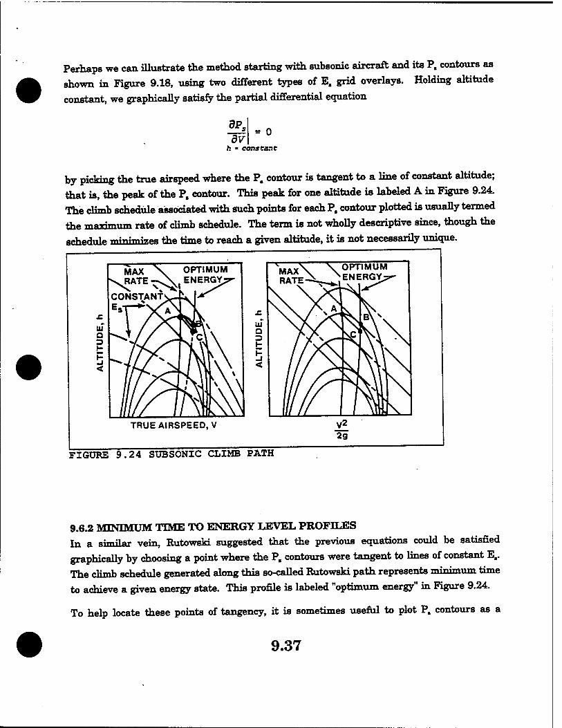
Perhaps we can illustrate the method starting with subsonic aircraft and its P. contours as shown in Figure 9.18, using two different types of E. grid overlays. Holding altitude

constant, we graphically satisfy the partial differential equation

3V -° h ■ constant

by picking the true airspeed where the P. contour is tangent to a line of constant altitude; that is, the peak of the P. contour. This peak for one altitude is labeled A in Figure 9.24. The climb schedule associated with such points for each P. contour plotted is usually termed the maximum rate of climb schedule. The term is not wholly descriptive since, though the

schedule minimizes the time to reach a given altitude, it is not necessarily unique.

OPTIMUM ENERGY;

OPTIMUM ENERGY: ^MAx\\

RATE-^

TRUE AIRSPEED, V

FIGURE 9.24 SUBSONIC CLIMB PATH

9.6.2 MINIMUM TIME TO ENERGY LEVEL PROFILES In a similar vein, Rutowski suggested that the previous equations could be satisfied graphically by choosing a point where the P. contours were tangent to lines of constant E.. The "litnh schedule generated along this so-called Rutowski path represents TniniTniim time to achieve a given energy state. This profile is labeled "optimum energy" in Figure 9.24.

To help locate these points of tangency, it is sometimes useful to plot P. contours as a

9.37

function of specific potential energy (h) and specific kinetic energy (V*/2g). Depending on the shape of the redefined P. contours, the points of tangency may be easier to choose with these

straight line E. contours. Of course, it is then necessary to compute the climb schedule

(obtaining V from V^g), rather than reading it directly.

9.6.3 SUBSONIC TO SUPERSONIC TRANSITIONS No matter what kind of plot is used, Rutowski suggested climbing along the optimum energy

path to C, which would put the aircraft at a specific energy level equal to that at A. However, the aircraft's potential energy would be lower with kinetic energy making up the

difference. Upon reaching C (in less time than that required to follow the maximum rate of

climb path to A), Rutowski assumed the aircraft would transition in zero time with no loss

in energy along an ideal zoom to A. It becomes immediately obvious why these transitions

are of such interest to Rutowski's successors in performance optimization; the potential gains

predicted by the energy approximation can be completely negated by the real process of exchanging kinetic and potential energies. In fact, for subsonic aircraft, the difference in the

two climb paths is usually within measurement error for flight test purposes.

However, for a supersonic aircraft, the energy approximation becomes much more

meaningful Figure 9.25 illustrates a typical climb schedule for a supersonic aircraft. The

path essentially consists of four segments to reach energy state E in minimum time. Segment AB represents a constant altitude acceleration from V= 0 to climb speed at state B. The subsonic climb segment follows a path similar to the one illustrated in Figure 9.24 approximately to the tropopause (state C). As a rule of thumb, this subsonic climb is usually a nearly constant Mach schedule. An ideal pushover or dive is then carried out at constant

E. from C to D. Finally, the supersonic climb segment from state D to KE is normally very close to a constant calibrated airspeed climb. Notice that this path is an idealized Rutowski

path except for the takeoff and acceleration to climb speed and the ideal (zero time) dive between states C and D. Segments BC and DE fit Rutowski's conditions by passing through

points on P. contours that are tangent to lines of constant E„.

9.38

MACH

FIGURE 9.25 SUPERSONIC CURVE PATH

Of course, there is a question of when and how to transition from the subsonic segment to the supersonic segment. The P. contours near M = 1 are poorly defined, and there is not complete agreement on when to start the pushover. Most analysts suggest flying toward the most expeditious path toward the highest P. contour available without decreasing E.. Such an assumption implies that one should climb subsonically until intercepting on E. level tangent to two P. contours of equal value - one in a subsonic region and the other in the supersonic region. Path CD in Figure 9.25 illustrate a typical transition following this reasoning. However, Figure 9.26 (9.6:17) illustrates rather well how difficult the choice of transition paths becomes when P. contours become irregular in the transonic region. The ideal climb path for the F-104G resulted in a time to 35,000 feet and M = 2.0 of about 194 seconds. This time compares to a time of 251 seconds for a subsonic climb at maximum rate to 35,000 feet followed by a level acceleration to M = 2.0 at constant altitude (9.6:18), a gain

of 23% in time to intercept.

However, before the rosy glow gets too bright, how about the story with real transitions as

9.39

opposed to ideal zooms and dives? Figure 9.26 shows a more realistic climb path with the "corners rounded off* -meaning that abrupt discontinuities in angle of attack and attitude were avoided in the actual climb. For one supersonic airplane, the ideal minimum time path to h = 65,000 feet and M = 1 took 277 seconds with zero time for dives and zooms. Using a more complete mathematical model, Bryson and Desai estimated 40 seconds for the dive and 60 seconds for the zoom for a total time of 377 seconds to the desired energy state. However, by treating V, h, q, and W as variables and controlling them with angle of attack, the same aircraft was estimated to require 322 seconds to reach h = 65,000 feetandM» 1 (9.1:483).

F-104G 1-fl SPECIFIC EXCESS POWER COMBAT WEIGHT - 18037 LBS CLEAN - MAX POWER - NO MANEUVER FLAP

FIGURE 9.26 F-104G MINIMUM TIME TO ENERGY LEVEL CLIMB PATH

9.7 FUEL OPTIMAL CLIMBS The energy approximation can be used to treat a number of performance optimizations other

9.40

than TwmiimiTTi time to climb. For example, if it is desired to expend minimum fuel to achieve a given energy level, the mathematical formulation of this optimization proposed by

Rutowski (9.2:192) is identical to the minimum time problem with appropriate variable changes. The objective is to increase total mechanical energy while conserving internal

energy (fuel) for future use.

9.7.1 FUEL EFFICIENCY To achieve the stated goal ("expend minimum fuel to achieve a given energy level"), we must define a measure of fuel efficiency that can be quantified. These words suggest looking at how much total energy is added to our mechanical system (the aircraft) per pound of fuel

burned. In symbols, our measure of merit is

Where Awf is the weight of fuel burned. In the limit

lim A£, = LEJL t = öEjdt = P, At-0 Awf Aw^/Afc dw£/dt w£

Usually, fuel flow rate can be treated as a function of h and V. The integral to be maximized

in this case is

W % * (9.14)

Since

dEB = Ps dt

and

dW = -vff dt

9.41

then

*=£ - -Et dw wf

(9.15)

the integral to be maximized can be written as

NT.

P, E= f -1* dW

(9.16)

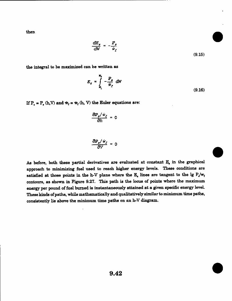
If P, = P, (h,V) and wf = wf (h, V) the Euler equations are:

dh

As before, both these partial derivatives are evaluated at constant E, in the graphical approach to minimising fuel used to reach higher energy levels. These conditions are satisfied at those points in the h-V plane where the E, lines are tangent to the lg P/wf

contours, as shown in Figure 9.27. This path is the locus of points where the maximum energy per pound of fuel burned is instantaneously attained at a given specific energy level. These kinds of paths, while mathematically and qualitatively similar to minimum time paths, consistently He above the minimum time paths on an h-V diagram.

9.42

MACH

FIGURE 9.27 MINIMUM FUEL TO ENERGY LEVEL CLIMB PATH

9.7.2 COMPARISON OF FUEL OPTIMAL AND TIME OPTIMAL PATHS Figure 9.25 illustrates a path similar in appearance to the time optimal paths of Figures 9.25 and 9.26. How do they compare for the same airplane? Figure 9.28 (9.7:118,124) answers

this question specifically for a clean F-105D at maximum power and is representative of the general case. Typically, as these data show, the fuel optimal path lies above but roughly parallels the time optimal path. Note that to reach the desired state (h = 45,000 feet and M

= 1.85) requires an ideal climb, an ideal dive, and an ideal zoom in the time optimal case. Hence, for this example at least, the fuel optimal path is closer to achievable reality than the

time optimal path.

9.43

60 -

" 40 x H U.

Ui Q

MINIMUM FUEL (VARIABLE FUEL WEIGHT) MINIMUM TIME (50% FUEL)

F-105D

MAXPWRVg CLEAN EMPTY WEIGHT

20,029 LBS 50% FUEL

5,040 LBS

0.6 MACH

FIGURE 9.28 COMPARISON OF TIME OPTIMAL AND FUEL OPTIMAL PATHS

9.8 MANEUVERABILITY Though we have defined and discussed maneuver energy, maneuverability in the sense of threenümensional trajectories has not been discussed. (Remember, maneuver energy is a measure of efficiency-fuel efficiency to be precise.) Now we need to re-examine the optimization problem with a view to extending the problem to include turning maneuvers. Indeed, several authors have used names like "extended energy management" (9.5:314) or "energy turns" (9.8:575). What we must do first is describe turning maneuvers and acknowledge at least two different types of maneuverability-both of which are related to

turning maneuvers.

9.9 INSTANTANEOUS MANEUVERABILITY Instantaneous maneuver capability is defined with use of the V-n diagram. A typical V-n

diagram is shown in Figure 9.29.

9.44

A-LIFT BOUNDARY B-STRUCTURAL LIMIT

er O H U < u. o < o

,,,,//*////////. C-q LIMIT

7777777777777777777//- B

CALIBRATED AIRSPEED, Ve

FIGURE 9.29 V-n DIAGRAM

Although a V-n diagram is published for most aircraft, the information contained in it does

not include the aircraft thrust capability which is necessary to determine sustained

maneuverability. Large multiengine cargo and trainer type aircraft are more concerned wxth

instantaneous capability.

The aircraft limitations shown on the V-n diagram are:

1. The lift boundary limitation

2. The structural limitation

3. The q limitation

9.9.1 LEFT BOUNDARY UMTTATION The lift limitation on turning performance refers to that portion of the flight envelope a which the aircraft is limited in angle of attack because of aerodynamic stall, pitch up, some form of a limits, or other factors, this is depicted by Curves A in Figure 9.29, the upper curve being in Ü» positive g environment and the lower curve for values of negative g. Every pomt along the lift boundary curve, the position of which is a function of gross weight, altitude, and

aircraft configuration, represents a condition of C^ or angle of attack limit. It is important to note that for each configuration, C^ occurs at a particular o^, independent of load

factor, i.e., an aircraft stalls at the same angle of attack and C\ in accelerated flight, n > 1,

as it does in unaccelerated flight, n = 1.

This area of operation is investigated through a test called the "lift boundary" investigation. Since this is primarily a problem in aircraft controllability, it is investigated in the Flying

9.45

Qualities portion of the course.

All aircraft can be flown to the lift boundary limitation in level flight in the low speed portion of the flight envelope. By combined diving and turning maneuvers, this limitation may be

explored through a large portion of the airspeed range.

9.9.2 STRUCTURAL LIMITATION Structural limitation is normally due to the aircraft limit load factor, which is defined as the

load factor where permanent structural deformation may take place or to the ultimate load

factor, which is defined as the load factor where structural failure may occur. Normally, the

ultimate load factor is equal to approximately 1.5 times the limit load factor and is a property

of the materials from which the aircraft is constructed. Limit load factors are indicated by

Curves B in Figure 9.29.

It will become evident that all aircraft, regardless of design or weight, will achieve the same

rate and radius of turn when maintaining the same velocity and load factor. Thus, when the

limit load factor is reached in flight, test can be discontinued, and the rate and radius of turn can be calculated for that portion of the airspeed range in which limit load factor can be

maintained.

Even among high performance aircraft, there is only a small portion of the flight envelope in which limit load factor can be maintained in level flight, although it can be achieved in

maneuvers such as dives and pullouts through a much larger portion of the envelope.

9.9.3 q LIMITATION q limitation is simply the TnaTrinrnm dynamic pressure the aircraft can withstand or the

ma-rim»™ flight velocity. The q limitation is shown by Curve C in Figure 9.29.

9.9.4 PILOT LIMITATIONS Another limitation which must be considered is the physiological limitations of the human

pilot. Although physiological limits have nothing to do with the V-n diagram directly, g limits on the human body have nothing to do with the V-n diagram directly, g limits on the

human body can be thought of in the same terms as g limits upon the aircraft.

If the pilot can withstand greater g-loads than the aircraft, he must always be aware not to exceed the aircraft limitations. If the aircraft can withstand greater g-loads than the pilot,

the pilot must always be alert to the possibility of gray-out or black-out when pushing the aircraft to the boundaries of the flight envelope. Naturally, this physical limitation will vary

with the individual pilot.

9.46

9.10 THRUST LIMITATIONS/SUSTAINED MANEUVERABILITY The thrust limitation on turning performance is the primary area of investigation in the

performance phase of flight testing. In stabilized level flight, thrust and drag considerations

will be the limiting factors through a large portion of the flight envelope. For combat flying,

this is the limitation on sustained turning ability without loss of energy (P, - 0). For aircraft

which are not expected to engage in combat, this phase of testing is of much less importance

and is generally omitted.

9.10.1 SUSTAINED TURN PERFORMANCE Sustained turn performance is very useful in establishing a fighter type aircraft's capability

for air-to-air combat. Once determined, this information can be used to compare an aircraft to possible adversaries. Unlike the V-n diagram, sustained turning performance analysis

includes the thrust capability of the aircraft. This performance is defined at the point where thrust equals drag in a level turn at a specified power setting (usually MIL or MAX power). We see then that aircraft sustained turning performance may be lift limited, structurally limited, or thrust limited depending on the aerodynamic design, structural strength or thrust

capability.

9.10.2 FORCES IN A TURN In a stabilized level turn, it can be seen from Figure 9.30 that the lift must be significantly

increased over that required for level flight.

9.47

FIGURE 9.30 FORCES IN A TURN

The greater the bank angle, the greater the increase in lift required. Naturally, an increase in lift produces an increase in induced drag. The increase in induced drag requires an increase in thrust to maintain the aircraft in a constant airspeed, constant altitude turn. The vertical component of lift is still required to offset the aircraft weight, and the horizontal component of lift is the force which is offset by the centrifugal force in the turn. The aircraft

experiences a centripetal acceleration toward the center of the turn.

To analyze mathematically the forces acting on the aircraft in Figure 9.30, we will consider an aircraft of weight (W) in a stabilized level turn of radius (R) with bank angle (*).

Since airspeed is constant, thrust equals drag, and forces in the X-Z plane are balanced. The

aircraft centripetal acceleration is given by V/R.

Summation of the vertical forces yields

T.FX = -L cos <|> + W = 0

9.48

L COS <f> = W

(9.17)

from which

L = 1 W cos 4>

But L

Therefore,

n = cos <t>

(9.18)

n is often referred to as the "cockpit g" as this is the load factor that the pilot sees in the cockpit. Note that n is dependent on the bank and is independent of aircraft type or configuration.

Summation of the horizontal forces yields

TFy ■ may

L sin 4> = may

but the centripetal acceleration is

9.49

Therefore

L sin ♦ = —-=■ 9 R

From the trigonometric identity cos2 <)> + sin2 + ■ 1, we can say that

L2 = (L cos <j>)2 + (L sin 4>)

using

L = nW ox L2 = nz W*

L cos $ = W or {L cos 4>)2 = W2

Lsin«.|-| or <*.!»♦>•-(*-£)'

and substituting

dividing through by W2 yields

9.50

(9.19)

(9.20)

n7 = 1 + W or

*»-!■+ V-

S2*2

from which

RZ= V gr'U2 - l)

and

j- ** gy/n2 - 1

(9.21)

which is the radius of turn and is seen to be a function of velocity and load factor. Minimum turn radius will be a function of the sustained g capability of the aircraft and the velocity.

Of note is the term -fif. which is know as "radial g" (n,). In the specific case of the level

turn, the radial g acts entirely in the horizontal plane. Recall that oo, the turn rate, is given

by a = V/R.

Substitution of Equation 9.21 into this relationship yields

(0 = ; V2/&Jn2 - 1

or

9.51

oas gyF^T

(9.22)

Equation 9.22 tells us that turn rate is also a function of load factor and velocity.

Solving Equation 9.22 for n yields

-^

a + 1

(9.23)

Equation 9.23 is a very important relationship used in turn flight testing because turn rate

can be measured directly.

9.11 VERTICAL TURNS It can be shown (left as an exercise) that for a vertical turn (zero bank angle) that the rate

and radius of the turn are:

v (9.24)

V2

g (n - cos 9) (9.25)

Where © is the angle measured from the upward vertical to the lift vector. As Equations 9.22, 9.23, 9.24, and 9.25 explicitly show, both turn rate and turn radius are related to normal acceleration. Thus, normal acceleration can be taken as a measure of merit for

turning performance.

For the practicing tactician, who really sees aircraft load factor on the g-meter, this measure of maneuverability also depends on orientation with respect to the earth's gravitational pull as shown in Figure 9.26. In other words, the acceleration of gravity can be used to "tighten up" (decrease the instantaneous radius and increase the rate of a turn) by maneuvering in the vertical plane. By comparing equation 9.25 with 9.21, we can come up with an equivalent

9.52

expression for radial g (n,).

n. = n - cos 0

(9.26)

The significance of these equations is in the fact that whatever the lift vector of the aircraft is below the horizon, the value of cos 6 is negative. Hence, the radial g (n,) is greater than the cockpit g (n). Of course, Equation 9.24 and 9.25 assume that the radial g act* along the vertical plane (i.e., single plane maneuvers). Figure 9.31 depicts the radial acceleration of

an aircraft executing a constant 4 g (cockpit) loop.

Poi-v* nr 0

A H 5

2*f 1*0*

C H «tf

» » <r

FIGURE 9.31. MANEUVER

ILLUSTRATION OF RADIAL G FOR A VERTICAL

9.12 OBLIQUE PLANE MANEUVERING

In dynamic performance testing, a topic that will be covered later in this course, a maneuver often performed is the wind-up turn or WUT. This maneuver results in combined plane turn with a continuously changing bank angle. As such, it would be beneficial to have an

9.53

expression for n, to apply to the basic form for turn radius ( R = v where x is an

gix)

expression for n,) in the case of the oblique turn.

Consider an aircraft in the turn shown in Figure 9.32.

FIGURE 9.32. OBLIQUE TURN SITUATION

Using the law of cosines we find:

n2 _ n2 + g2 _ 2ng cos 4>

since g=l

nz = \Jnz + 1 - 2n cos

(9.27)

Plugging this value into the equation form for turn rate and radius, we get

9.54

_ gj {n2 + 1 - 2n cos <|>) v

V2

(9.28)

g\/{n2 +1 - 2n cos <f>) (9.29)

Note that in the case of the level turn, this equation still applies as the term 2n cos<{> approaches a value of z. That is, at low values of <)>, very little n will be needed to maintain level flight. As $ (and hence cos <j>) increases, the value of n will have to increase to sustain

level flight. Hence, the expression for n, reduces to Jnz _ ] .

So, what is the significance of this to the individual accomplishing performance testing? First, aircraft turn performance will be evaluated using level turns and then expressed as a function of radial g (n,). Second, as test techniques such as the wind-up turn are discussed in dynamic performance testing, it will become apparent that bank angle ($) and pitch angle (0) will have an effect upon, and therefore need to be accounted for, in the determination of aircraft acceleration. Finally, as you progress into the Flying Qualities phase and examine maneuvering flight, the understanding of radial g will help you to understand the different values of stick force per g received by using the various flight test techniques.

9.13 TURNING PERFORMANCE CHARTS Combining the relationships for turn rate and turn radius yields a chart such as Figure 9.33. As true airspeed (V), gravity (g) and cockpit load factor (n) are the only variables needed to determine oo and R, this chart is independent of aircraft type. If, in fact, the chart was © as a function of V, it would be good for all altitudes. But, due to the use of Mach as the independent variable the chart becomes good for only one altitude.

9.55

10,000 FT

MACH FIGURE 9.33. TURN RATE - TURN RADIUS RELATIONSHIPS

Overlaying a P. = 0 curve for a particular aircraft onto Figure 9.33 makes the chart aircraft specific and will yield three Mach numbers of interest as illustrated in Figure 9.34.

9.56

EIGOKS 9.34. TORN RATE/MDIÖS P. OVEBIAI

The point where *e P. = 0 curve is tangent to a cenatant load factor hue (Pen* a ur F*ure 9.34iyielda tie Mach for »axtann suatained g for W configuration. The F-"*> P = 0 curve (Point b in Figure 9.34) yield» the Mach for maünrnm turn «to, and the pomt where the P = 0 curve is tangent to a value of conetant turn radius (Pomt c m Figure 9.34)

9.57

is the Mach for minimum turn radius. For most cases

*4_ > M«» > M, ̂

in

Although in „me aircraft, at certain altitude», the Mach value for magnum «. rate and „stained g may occur together. An example of this «ee la ahown in Figure 9.35.

By evaluating P. value, and overlaying them on the tun. rate-radiu. chart, a graph of! tie 4 in Figure 9.35 (for the F-15C) ia priced to define an aircr.fi?. a^amed turn capthmtieTah. method, hy which thi» graph «produced will be preaented later m the

course.

"F-15C

TURN RRTE VS MACH

KCRS

CONFIGURATION:

50* INTERNAL FUEL 4 B'lt-7 ♦ e Sin-9 wuimm n/B POME*

RLT =10000. WEIGHT=40095. 01 =23.80

Tj.00 O.'O 0.80 1-2° MACH NUMBER

40

llGURE 9.35. F-15C TURN RATE VERSUS MACH AT 10,000 FT

9.58

From this example, the following points concerning sustained turns can be noted:

1- Mn^ occurs between 0.87 and 0.96 Mach (maximum sustained load factor equals

7.33 g) 2. M_ occurs at 0.87 Mach (maximum sustained turn rate equals 13.0 deg/sec).

HMUC

3. Mr, occurs at 0.34 Mach (minimum sustained turn radius of 2200 feet). "min

In addition, the turn rate-radius versus Mach plot shows the maneuver or "corner" point. It is denned as the wmi«mm speed at which the maximum aircraft load factor (n) can be achieved. On the V-n diagram (Figure 9.29) it is located at the intersection of the lift boundary (line A) and structural limit boundary (line B). In Figure 9.35, it occurs at the intersection of the max lift line and the maximum load factor line. In this case, the corner point is at 0.55 Mach, pulling 7.33g and achieving approximately 23 deg/sec turn rate. Notice that this equates to a P. value of less than -2000 ft/sec. To the pilot this means a loss of Mach at constant altitude pr a loss of altitude at constant Mach to hold 7.33g. Hence this is often noted as the mayiirmm instantaneous turn capability of the aircraft and the term "quietest, tightest turn" is used in the fighter community to describe the aircraft performance

at that point.

By «"^mining the P, = 0 plot in Figure 9.35, it can be seen that for each level of load factor there are two Mach values where the aircraft can stabilize. This may be better visualized

by analyzing Figure 9.36, which shows that by increasing -^ for a given, the speed at

which these stable points occur come closer together. And, at some point, there is a load factor that can be sustained at only one speed.

9.59

Fn (MIL)

SÄ OR © IF^= CONSTANT

rMIN

CALIBRATED AIRSPEED, Vc

FIGURE 9.36. FACTORS AFFECTING TURNING PERFORMANCE

Figure 9.36 implies that a graph of load factor as a function of Mach for a sustained turn, p _ o (Fa m D), would look like the upper plot of Figure 9.37. Once load factor is known, to

and R can be calculated. Typical results are also presented at Figure 9.37.

9.60

tu

cc z cc D

0) 3 5 < CC z cc

MAX

MAX

He- CONST W-CONST

F„« CONST

FIGURE 9.37. SUSTAINED TURN PERFORMANCE RESULTS

Thus, turn rate, turn radius, and radial acceleration are very important parameters, along with P., in comparing relative performance of maneuvering aircraft. Such comparison, derivedfrom the energy approximation, are of extreme interest to designers, operators, and

test personnel.

9.61

9.14 THRUST LIMITED VERSUS LIFT LIMITED

TURNS An additional concept to be discussed in turn performance is that of limited turns. There are

two types of limited turns...thrust limited and lift limited.

The thrust limited turn is one in which the aircraft thrust is insuffident to maintam Return

up to the lift limit of the wing. The lift limited turn is one in which the thrust capabüxty to sustamaturnexceedsttecapabmtyoftiiewingtogeneratelift. Thebestway to show tins

is with a V-n diagram. Although a V-n diagram does not, by the strictest definition, show the sustained turn capability of an aircraft we can superimpose a P. = 0 curve to demonstiate

the difference between thrusted lift limited turns. Figure 9.38 shows two P. curves plotted. Note that P. = 0 plot A extends to the left of the lift limit boundary. In essence, tins shows that A at a given load factor, would be accelerating as the aircraft stalled. Whereas the P. = 0 plot of B indicates that at the same load factor the aircraft would be a negative P. = 0

////////////////, _.

77777777777777777777/-

CALIBRATED AIRSPEED, Vc

FIGURE 9.38. LIFT VS THRUST LIMITED TURNS

when it reached the stell. In other words, the thrust limits our sustained turn capabikty in situationB.andliftlimiteoutsusteinedturncapabüityincaseA. To determine the hmxting

factor of the aircraft, you must examine which parameter, at a given airspeed, xs reached first (stall or P = 0) at a set load factor. If, at 300 K3AS and 10,000 feet pressure altitude, you attempt to make a stabilized airspeed military power level turn and at 3 g you find you are

9.62

holding your airspeed then this is a thrust limited turn. If, with the same initial condition, you find that the airspeed is increasing and you reach an accelerated stall condition at 5 g

before you can stabilize the airspeed, then this is a lift limited turn.

9.15 SUSTAINED TURN PERFORMANCE FROM LEVEL ACCELERATION The final topic on turn performance is the completion of sustained turn capability from a level acceleration. To provide a basis for the underlying principle, well start with a little

review of aerodynamics.

For a sustained turn, thrust equals drag. Thrust is normally fixed at either military or

maximum power, but does vary according to the relationship

■S - f (M. N/y/B

Where Fn = Thrust

8 ss Pressure Ratio p

M =Mach

-^ = Normalized RPM ye

e T - a

««i

The drag increase in a sustained turn is strictly induced drag due to the increase in lift

required to sustain level flight. Therefore, we can write

AD - ADp + AZ?i

but

9.63

and

also

or

where

For a given weight

Therefore

Recalling that

AZ?p- 0

&DX = AC« qS

AC = (AC^)2

LcDi = *{A c£f

JC« 2

n AJ2 ©

AL . An . A^£ w tf

ACL- A^r

9.64

and that

or

But q can be written

Therefore

A^ = ACDi qS

AC. = K (AC,)8

A«%.-*W

Ant^2 An . jc ii^I "gs im2

An -K" (Any)2

g = 1481 d M2

An = * 1 / AflWA* *D* 1481 5 6 I M )

or

9.65

An .^i (AnW\2

where

K Ki - 1481 S

Dividing both sides of this equation by 8 yields

-r" ^ -TO") (9.30)

From Equation 9.30, we can see the relationship of n, W, and M on induced drag. More importantly, it gives us the basis for determining sustained turn performance.

The determination of turning performance through a level acceleration test first requires

calculation of energy height from the relationship

V2

2g

Differentiating E, with respect to time yields

■ dEs _ dH ^ V dv E* dt dt g dt

which you recall is the definition of specific excess power, P..

Since the level acceleration is performed at a constant altitude

M = o dt

9.66

The aircraft is accelerating. Therefore,

but

from Equation 10.11. Therefore,

F = — a ■" g *

g v

or

F*c ~ ~y Es

Computers are normally utilized to determine E,. However, if a computerized data reduction system is not available, E. can be determined graphically. E. and V can be plotted as functions of time for the duration of the level acceleration test run as shown in Figure 9.39.

9.67

FIGURE 3.39. GRAPHICAL DETERMINATION OF E.

For each At, the slope of the curve AE/At or E. can be determined. Similarly, AV/At = V

a,. Excess thrust for a given velocity is then readily determined from

WE* - constant Vt = constant

and can be normalized be dividing the pressure ratio, 8.

Since the test must be performed at several altitudes, FJ* must be plotted as a function of

Mach for each altitude as shown in Figure 9.40.

9.68

FIGURE 9.40. NORMALIZED EXCESS THRUST VS MACH

From figure 9.40 and Equation 9.30, FJ5 can be plotted as a function of (nW/5M)2 at a given

Mach and at n = 1 as shown in Figure 9.41.

9.69

M, H,

M, H» PROJECTION TOWARDS

P.-O

^4r =+" [buj

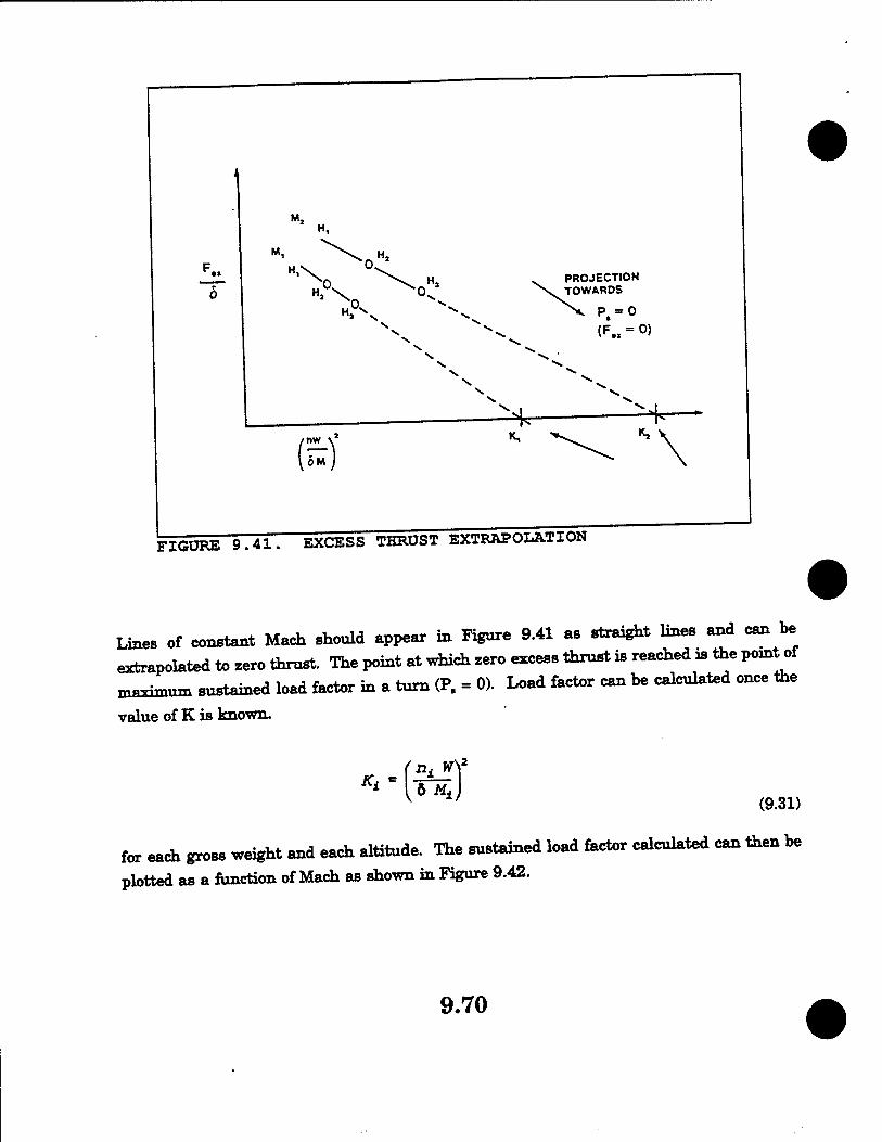
FIGURE 9.41. EXCESS THRUST EXTRAPOLATION

Lines of constant Mach should appear in Figure 9.41 as straight lines and can be extrapolated to zero thrust. The point at which zero excess thrust is reached is the pent of

maximum sustained load factor in a turn (P. = 0). Load factor can be calculated once the

value of K is known.

K< - 6 HA (9.31)

for each gross weight and each altitude. The sustained load factor calculated can then be

plotted as a function of Mach as shown in Figure 9.42.

9.70

FIGURE 9.42. SUSTAINED g VS MACH

Turn rate (to) and turn radius (R) can be obtained from Equations 9.21 and 9.22.

Two limitations of the level acceleration method are: 1. The thrust component due to angle of attack is not accounted for. 2. Engine lag characteristics during acceleration are unaccounted for.

The net result of these limitations is that the values for sustained load factor will be slightly

lower using the level acceleration method than the stabilized turn method.

9.16 DYNAMIC PERFORMANCE TESTING

9.16.1 INTRODUCTION

The most current form of performance testing available today is dynamic performance testing. The ability to determine an accurate installed engine thrust deck for an aircraft by using either the Pressure Area Method or Mass Flow Method provides for direct calculation of lift

and drag at a given Mach number.

9.71

For the Flight Test Engineer, assessing aircraft performance, the output desired from the test generated CJCj, plot, similar to the one shown in Figure 9.43. Once this plot has been is a

produced, then (assuming that the thrust deck is accurate) cruise, turn and acceleration

MK:-!S5A \SSSC S/K.S5-312S . : i-S-t-O« V&Xl . .

. I e.?e no! ; -. i J6SM FT! :

1 •>-

. CO-- <3?

■<&

cS^C

; ■ i ^J.4^-i_...--L..,.^,:.

-;; T"3Tn

_. Co ; —i-Ä!—i— ;-35»i : i ■•

l/'.4>jViai»ta* '• wi« *U. i ':

* T?^t

f <SV'A£ // •::: iBgASPOUi.J ! : •: - r ' r'-"T-. ■" .

FIGURE 9.43. KC-135 Cj./Cp PLOT AT 0.7 8 MACH

performance can be accurately modeled. In past years, the construction of an accurate thrust

deck was the limiting factor in performance testing. As a result, performance data was collected using methods devoid of the requirement to accurately measure installed thrust. However, today installed thrust can be modeled very accurately. In fact, on the X-29 project they were able to obtain real-time thrust values to within 3-5% using 8 different telemetered

pressure measurements.

So to understand dynamic performance testing in concept and practice we will work backwards from the desired results to the aircraft parked on the ramp. To begin with,

consider the aircraft shown in Figure 9.44.

9.72

FIGURE 9.44. KC-135 FORCE DIAGRAM

Summing forces perpendicular to the fight path (a^-wind axis):

T.FZ = maz = N W = L + Fg sin (a + ot)

L - qSCL

[NT W - F- sin (a + oe)3 C - —Ü" '* as

(9.32)

and summing parallel to the flight path:

9.73

HFX = max = NXW = Fg cos (a + at) - F9t - D

D = gSCD

■F»t = ^x«m + Fspi.llag* + Fnorzlm

F„ = F_ cos (a + ot) - F, •t

F.„ = JV, W - FB - qSCn

qS (9.33)

Where: Fg = gross thrust Ot = thrust inclination angle

-q = dynamic pressure

S = wing area F.* = excess thrust F^n = engine ram drag F.PÜ1V, = engine spillage drag Faoai. = engine afterbody drag Fn = net thrust (gross thrust corrected for engine related drag, along the

X-axis)

9-74

From Equations 9.32 and 9.33 we now have expressions for C,, and Cj,. Assuming a non-

active wing, S will be know and constant. The value of q can be calculated and W

should vary with fuel bum, but will also be measurable. Values for a can be obtained and a, is easy to measure. Again, we assume a good thrust model so F, is known. Although a form of drag, Frt is something that can be evaluated. This leaves the values of N^ and NXw

as unknowns.

9.16.2 MEASUREMENT TECHNIQUES

How can these be measured? There are 3 methods: eg (or body axis) accelerometers, flight

path accelerometers (FPA) and inertial navigation systems (INS). Figure 9.45 graphically demonstrates each method. With the eg accelerometer, the accelerometers are strapped down to the body axis and sense accelerations along the longitudinal axis, perpendicular to the longitudinal axis, and along the lateral axis of the body. The flight path accelerometer places

the accelerometers on a gimbaled platform at the end of a nose boom attachment. Accelerations are then measured relative to the flight path Finally, inertial navigation systems may be used to gather the accelerometers. The INS is strapped down and velocity

measurements are taken in the inertial reference frame.

9.75

FIGURE 9.45. MEASUREMENT TECHNIQUES

In general, each of these methods of measurement will generate the values of N^ and N^ required to calculate the coefficients, Cp and C^. However, the various transformations and corrections required will depend upon the type of data collection device. Consider that, in dynamic performance testing, the aircraft will fly a non-stable flight profile. One such profile is the push-over pull-up, or POPU. The profile looks as shown in Figure 9.46.

9.76

**ck - k.

LO&&IU&

FIGURE 9.46. POPU MANEUVER

As you can see, the aircraft undergoes a sweeping of a and, consequently, a variation of pitch

rate (q). When the maneuver is flown it is done so such that the rate of change of a is not

excessive but sufficiently large enough to allow the maneuver to be accomplished while ^^„iT^e- constant Mach. Because this is a dynamic maneuver, some corrections will have

to be made.

9.16.3 CORRECTION AND TRANSFORMATIONS

Consider the example of the KC-135 Winglet Test Program, which accomplished dynamic performance test using FPAs. Some of the corrections required included:

PITCH RATE CORRECTIONS TO a: Because the aircraft is pitching, an error in the value

of a will occur (increase for nose-down pitching, decrease for nose-up pitching). This error

will manifest itself not only when establishing the a for the independent variable of the plot/computation, but also in the reading for Nx and N. obtained for the false a (the FPA is

misaligned).

ACCELEROMETER RATE CORRECTIONS: Placing the accelerometers at the end of a nose

boom will result in the measurement of not only the accelerations of aircraft, but also the

accelerations due to the rotation of the aircraft about the eg. This rotation causes the

introduction of centrifugal acceleration parallel to the aircraft body axis.

9.77

LOCAL FLOW CORRECTIONS Local flow corrections are simply corrections to both a and accelerations due to "upwash."

It is left to the reader to determine methods of accomplishing this.

BOOM BENDING As the FPA is mounted at the end of a boom, under load the boom will be subject to bending and hence, the accelerometer values will be in error. This bending will require the

application of corrections.

If working with an INS, a transformation will be required to change the inertia velocities in the inertial reference frame into* accelerations referred to the wind axis. These transformations tend to be quite complex in appearance, but can be quite easily solved with

computer assets available at the AFFTC.

In order to complete the process of presenting dynamic performance using the KC-135 example, let us assume that the aircraft was fitted with eg accelerometers. Since the accelerometers are placed on board the aircraft along the body axis, a transformation must

be used to convert the values of N^ and N^ to N^ and N^.

The transformation used would be:

Nx = cosß {Nxcosa - i^sina) + fl^sinß

N = -sinß (Nx cosa - Nr sina) + Ny cosß

(9.34)

(9.35)

N = N, sine + Nz cose

(9.36) Notice that in equation 9.34 and 9.35 there is a factor for sideslip angle (ß). In the case of the POPU, if the maneuver is flown perfectly the value of sideslip should be zero. This simplifies the equations to a consideration of N, and N, alone. Now that the eg accelerometers values are corrected, we have all the data required to compute Q, and C„. Therefore, for each value of a evaluated, there will be a corresponding (^ and, hence, Cj,

value that may be plotted against each other at a specific Mach and altitude.

The obvious limitation with the POPU maneuver is that you are limited in the amount of a that may be swept during the profile. Why is that so? In order to maintain the constant

9.78

Mach value required by this test, an aircraft would be extremely limited in the amount of nose-down and nose-up pitch altitude it could obtain. Therefore, transport aircraft typically achieve no greater than N, = 1.5 and fighter aircraft top out around N, = 2.0 (although the F-15 CTF conducted POPU profiles up to Nz = 5.0). The equally obvious advantage of the POPU is the ability to sweep to values of NM < 1, thus, obtaining C^ for the C^ = 0 state (Cj) ). In order to obtain values for N, nearing the limiting g of the aircraft, which in aircraft likePthe F-16, Mirage 2000. and F-18 is up to 9g, a different flight profile must be used. For these data point values the Wind-Up Turn (WUT) a Split-S (SS) maneuver is used. Each of these maneuvers will be discussed later in this chapter, but for a physical interpretation of this type of test, let us examine the aircraft accomplishing a WUT. The aircraft we will use will be the F-4 and F-16. The WUT is a descending, constant throttle, constant Mach turn of increasing Nr Suppose that both aircraft are flying 0.8 IMN at 20,000 ft pressure altitude. A comparison of each aircraft CJCD curve might show something similar to that of Figure

9.47.

FIGURE 9.47 C^/Cu COMPARISON

This is intuitively apparent as the F-4 design has quite a bit more drag than the F-16. Thus, if both aircraft begin a WUT with the same on set rate (given same aircraft weight) the F-4 will experience a much higher value for CD- From the standpoint of the outside observer, the F-4 would have a greater nose low altitude in order to hold the constant Mach profile. The engineer gathering data would observe that although both aircraft were reading the same value for N , the F-4 would have a value for N^ significantly higher than that of the F-16.

9.79

9.16.4 CONCLUSION In conclusion, the obvious significance of dynamic performance testing is the ability to

accumulate vast amounts of performance data from one maneuver. Rather than accomplish

a large series level accelerations, stabilized cruise points or constant airspeed/constant g

turns, a smaller number of POFUs, WUTs or SSs may be flown. Use of these techniques may

reduce hours of flight test required by up to 50%. In practice, a number of the "older" tests will be required to validate the performance model established by the results of the dynamic performance tests. However, this number will be small It is not important that you know

all the transformations that have been presented. Rather, as it is the predominant

performance test method used today, you should have an idea ofthe process involved.

9.17 DATA COLLECTION FOR ENERGY METHODS

9.17.1 INTERNAL MEASUREMENT TECHNIQUES One of the strengths of the energy methods is the variety of means available for data

collection. Pitot-static data, if accurately calibrated and correlated with time, can give the basic information. Of course, for real time profile management displays or feedback

information for automatic flight path control, one must have corrected air data as well as acceleration sensors of considerable precision and sensitivity. Evaluation of such systems

requires careful planning on the part of the flight test engineer, with careful note taken of the range, precision, and dynamic response of the required flight test instrumentation.

9.17.1.1 PRESSURE METHODS Sometimes called airspeed/altitude (A/A) methods, the collection (and correction) of pitot-

static data has been rather completely discussed, since these data are available in one form

or another on any military aircraft and since they have been collected and used form the very beginning of flight, pressure data must be considered one of the most readily available sources of data. The required aircraft system for data collection, however, is not always

suitable as flight test quality data. Sensitive instruments and panel vibrators, for example, are often needed to provide usable airspeed/altitude information. Further, some form of

numerical differentiation, which is an inherently inaccurate process, must be carried out to

get accelerations and rates of climb or descent But for a rough estimate of an aircraft's

energy capabilities the production instrumentation will suffice.

9J7.1.2 ACCELERATION MEASUREMENTS There are at least two very accurate devices for measuring performance on board the aircraft. Changes in energy states are readily available from the eg accelerometer flight path

accelerometer (FPA) and/or inertial navigation systems (INS). Both have been and are being

9.80

used extensively since 1973 to collect energy data. Both techniques are very accurate and quite reliable, but subject to some of the errors discussed in 9.16.2. Nearly all of the INS systems used are production systems, not installed as flight test instruments. The alignment

calibrations are done by INS manufacturers to meet the rigid navigation specifications. Both

these techniques measure accelerations and rates directly, and numerical integrations produce position (potential energy) data instead of numerically differentiating to arrive at

rates and accelerations. The INS is considered the most accurate internal method, followed

by the FPA and eg accelerometers.

9.17.2 EXTERNAL MEASUREMENT METHODS So far only internal methods of measurement have been discussed. There are methods

available for determining aircraft performance wing ground-based systems. These systems,

collectively, are called Time Space Position Information or TSPI. There are a number of ways to directly measure position in space, and they can be used to obtain energy state and energy

rate.

9.17.2.1 RADAR TRACKING Radar tracking (RT) is a very common method, and it has been in use for a number of years. While it requires a moderate amount of data reduction including transformations for both

rates and positions as well as wind corrections, it is a relatively cheap and not very accurate technique. Errors in radar measurement are typically up to 25.0 feet in position, 2.0 ft/sec in velocity and 2.0 ft/sea, in acceleration. Compounding these drawbacks is the relatively low

availability of flight test quality radar data except on highly instrumented ranges.

9.17.2.2 OPTICAL TRACKING (OT) OT is also a means of obtaining usable position information. No on board transponders or computing devices are necessary. It is less available than radar and is located only at a few sites. Such devices are limited by weather conditions and are generally used for shorter

ranges. It is fairly accurate, better than radar, but not comparable to laser devices. Optical tracking is commonly referred to as Cine tracking. Accuracies are up to 3.0 feet in position,

0.5 ft/sec is velocity and 0.5 ft/seca in acceleration.

9.17.2.3 LASER TRACKING <LT) The pure LT has been around for quite some time. Although not extensively used in the USAF, other services and nations use this type of tracking system. The accuracy of LT systems is close to that of Cine, approximately 1.0 ft in range, 0.5 ft/sec in velocity and 0.5

ft/sec2 in acceleration.

9.17.3 MODERN METHODS

9.81

Two new methods have begun to appear in the test community. The first is the use of Global Positioning System (GPS) units. The GPS incorporates a receiver and a network of transmitting satellites. Through triangulation, an accurate position of the aircraft may be

derived. The major advantage of this type of system is that it allows a test to be conducted anywhere in which the receiver can pick up a sufficient number of satellites. Thus, the aircraft is no longer tied to a range in order to achieve accurate results. Three types of GPS

are available:

1. GPS-NS (Navigation Solution): This method uses only the on-board GPS navigation solution to obtain position, velocity and acceleration. No smoothing technique is used on the output from the receiver. With this system, accuracy is limited to no less than 12.0 feet in

position, 0.3 ft/sec in velocity and 0.3 ft/sec2 in acceleration.

2. GPS-TE (Trajectory Estimation): This method uses the raw position and velocity measurements as input to the trajectory estimation rates. The net result is an overall increase in the accuracy of the solution With this type of system, the accuracy is limited to no less than 9.0 feet in position, 0.3 ft/sec in velocity and 0.3 ft/sec2 in acceleration.

3. GPS-BET (Best Estimate of Trajectory): This method is similar to GPS-TE except that it combines GPS measurements with all the other sources for positioning available. The net result is enhanced accuracy up to 3.0 feet in position, 0.2 ft/sec in velocity and 0.2 ft/sec2 in

acceleration.

Another method is the use of Lasers for ranging in conjunction with a contrast tracker. This gives two methods by which to position an aircraft and therefore increases the accuracy of the output. This type of system is being used by the US Navy.

9.17.4 RELATIVE MERITS From the preceding discussion, it should be clear that no single means of taking energy data is superior for all aircraft and all time. The choice of measurement is one of the many engineering judgments based on the intended use of the data, the available equipment on the test article, the cost of the instrumentation, the need for reliability, availability, and the time

and money available for data processing.

9.18 CLIMB AND DESCENT TESTS The tests that are associated with the determination of the climb performance of an aircraft will now be explained. The climb performance is determined from an airspeed schedule, and the first order of business is to determine that schedule. Lower performance aircraft can use the sawtooth climb method for climb speed determination. The level acceleration method is

9.82

more suitable for high performance aircraft.

Once the climb speed schedule has been determined, the actual climb performance of the

aircraft is obtained by running check climbs to altitude. In general, the same procedure is

used for both reciprocating engine and jet aircraft. The factor which complicates climb performance determination is the fact that all data must be corrected to standard day conditions. Test day performance is easily obtained but has no meaning if used to compare two aircraft flown on two different days. It is therefore necessary that sufficient data be

recorded and proper techniques employed to reduce the results to standard day conditions.

The most important factor is nonstandard temperature, from a performance standpoint.

Other corrections such as those for nonstandard weight, vertical wind gradient effects, and

climb path acceleration are normally of lesser importance.

Since large lag errors occur in the measurement of the free air temperature, the temperature as obtained from a weather station may be satisfactory and is sometimes more accurate than that obtained from the aircraft instrument when insufficient time has been allowed for

stabilization.

9.18.1 SAWTOOTH CLIMB TEST The sawtooth climb test is one method of obtaining the airspeed schedule for maximum rate

of climb. Its name is derived from the barograph trace resulting from a series of short,

timed climbs through the same pressure altitude band (as shown in Figure 9.48).

FIGURE 9.48 SAWTOOTH CLIMB

This test provides little or no useful information on climb performance. It merely establishes

9.83

the best airspeed at which to climb.

Essentially, this test employs a trial and error method. A series of timed climbs is made at

different speeds from a point below the test altitude to a point above it. Speeds are chosen to bracket the expected best climb speed of the aircraft.

Climbs are performed at the same power setting and aircraft configuration as will be used

in the check climb. The -altitude increment should be chosen such that the aircraft will

traverse it in about one minute. Smaller time increments will introduce excessive scatter in

the data.

The aircraft is first trimmed in the climb configuration while still well below the nominal

altitude. Power is applied and final trim adjustments are made before reaching the lower

limit of the altitude band being measured.

The exact time of entering and leaving the altitude band is recorded by stopwatch or

instrumentation system.

Upon emerging from the altitude increment, data are recorded, and a 180° descending turn

is initialized to bring the aircraft below the altitude band for another run. As many points

as possible should be flown at each altitude. In addition, a full power unaccelerated minitnnm speed point and a maximum speed point should be obtained at the test altitude in order to complete the curve. These latter two points should be flown at the beginning of the

test so that weight corrections will be minimized.

An effort should be made to confine the flights to the bounds of a limited geographical area since the primary concern is the shape of the curve obtained rather than the magnitude. If

the aircraft remains in this area, the effects of lifting and atmospheric conditions should be minimized. For each altitude, a standard data card should be prepared with the aim

indicated airspeed (aim V,) included for each point. Provision should be made for recording in flight actual V„ W, time, fuel counts, and either outside air temperature or time of day.

On the back of the data card, a running plot of observed time to climb versus Vt should be

kept, and before leaving the test altitude, it should be examined for points that might need

repeating.

9.18.2 LEVEL FLIGHT ACCELERATION TEST With the advent of high performance aircraft, the performance envelope has greatly

expanded, and additional areas of investigation have become important. Higher wing

9.84

loadings require higher wing speeds, and the acceleration from brake release to climb speed assumes greater importance. Supersonic capabilities result in a wide differential between best climb speed and maximum level flight speed, and the level acceleration performance at altitude becomes important. For most supersonic aircraft, a supersonic climb speed schedule

is of interest in addition to the familiar subsonic schedule.

The level flight acceleration test serves two purposes. It makes available acceleration time

and fuel consumption data in level flight, and it may be used for determining climb speed

schedules both subsonically and supersonically.

9.18.2.1 METHOD Level flight accelerations from near minimum to near maximum airspeeds ar normally flown at a variety of altitudes. As in the sawtooth climb test, power settings and aircraft

configurations are those which will later be used in the check climb, since a number of simultaneous readings are required and since data points are only a few seconds apart,

recording should be mechanical, usually by Data Acquisition System (DAS). However, m aircraft unequipped with such a system or during qualitative evaluations, data may be taken

manually using a tape recorder or data cards.

Values of indicated airspeed and time are the primary parameters. Fuel flow and free air temperature data are recorded, and indicated altitude is included so that errors caused by

climb or descent may be corrected.

9.18.2.2 PREFLIGHT PREPARATION A mission card should be drawn up, and entries should be recorded in order that correlation

between runs, power settings, time of day, etc., may be facilitated. Required entries include:

1. RUN NUMBER 2. ALTITUDE 3. POWER SETTING (MH OR MAX)

4. RPM 5. TIME OF DAY.(TOD) 6. COUNTER NUMBER (START AND FINISH)

7. FUEL (START AND FINISH)

Any other desired parameters not included on the DAS may be recorded as necessary.

The level acceleration will be flown level at a constant tapeline altitude, that is level in

reference to a datum altitude based upon a 29.92 in Hg pressure setting. In order to minimize errors it is necessary to fly this constant altitude. However, as the aircraft

9.85

approaches transonic flight pitot-static errors are encountered that result in erroneous displays. Therefore, the pilot should make himself familiar with altitude position error corrections of the aircraft so that he can plan for a slight indicated rate of climb or descent

which will result in a nearly level flight path.

Q 1 ft 9 ^ TT^JF^J

The'level flight acceleration is the method used to obtain climb schedules for high

performance aircraft chiefly because:

1 It is relatively easy to obtain good data at values of P. where climb rates would be

too high for accurate sawtooth climbs. In fact, the data accuracy improves at higher values

of P..

2. Flying time required is much less than for the sawtooth climb. Usually one-half

the time or less will cover the same speed and altitude range.

3. Wind gradient errors are smaller.

4. Acceleration data is obtained in conjunction with climb speed data.

5. Supersonic climb speed schedules can be found by this method.

9.18.2.4 LIMITATIONS 1 At low climb rates, the peaks of the curves are poorly defined. Thxs limits the

usefulness of the method for low performance aircraft and for any aircraft as it approaches

its service ceiling.

2 Data reduction processes are tedious if a hand reduction method is used.

Computer data reduction programs reduce the time considerably, although loading the raw

data can still be tedious.

3. Unless some form of mechanical recording device is available, data cannot be

collected rapidly and accurately enough to be of value.

4 Because scatter is always fairly high, a single level acceleration is not reliable.

From two to ten or more runs at any altitude are required to properly define the curve.

918.3 CHECK CLIMB TEST FOR JET AIRCRAFT The check climb test is flown to evaluate the standard day climb performance of an aircraft

in a specific configuration. The three main areas of investigation are:

1. TIME TO CLIMB

9.86

2. DISTANCE TRAVELED

3. FUEL USED

In addition, data may be obtained on various engine parameters such as engine speed,

exhaust gas temperature, engine pressure ratio, gross thrust, etc. These are useful to the

analyst but are secondary to the three main parameters. The general method is to climb the

aircraft to just below the maximum ceiling while mamtaining precisely a predetermined climb schedule. This schedule may be a best climb schedule as obtained by flight test, a schedule recommended by the manufacturer, or some other schedule for which climb performance is of interest. Care should be taken to specify on each climb performance chart the schedule

flown.

Data should be recorded at approximately equal increments of altitude and should include

time, speed, fuel used, temperature, and any other desired parameters. For most jet aircraft, a mechanical recording means will be necessary to obtain simultaneous reading of the many

parameters of interest.

9.18.3.1 PREFLIGHT PREPARATION The data card serves a double purpose; it provides the pilot with a list of aim speeds for each altitude and is used to record pertinent data facts. The first portion of the data card is used to record fuel used to start and taxi, and fuel and time required to accelerate from brake

release to climb schedule.

Aim speeds should be adjusted for instrument error and position error of both the airspeed

indicator and altimeter. If the anticipated rate of climb is low, airspeeds would be presented

every 1,000 or 2,000 feet with speeds to 1/2 knot. If the rate of climb is high, every 5,000 feet is sufficient with speeds to the nearest knot. It may be advisable to decrease the interval to

every 2,500 feet or 2,000 feet as the rate of climb decreases with altitude.

Perhaps the most difficult step in obtaining good check climb data is finding an area of satisfactory meteorological conditions. An area of smooth air, light winds, and stable temperature gradients from ground level to the aircraft's maximum ceiling is desirable. A survey balloon should be sent up before the flight for wind and temperature data and an area

chosen where the climb can be performed at 90° to the average wind direction.

Since aircraft gross weight and fuel density are extremely important, arrangements should be made, if possible, to weigh the aircraft fully fueled immediately prior to takeoff. In any case, fuel samples from the tanks should be taken to obtain fuel temperature and density.

9.18.3.2 FLIGHT TECHNIQUES

9.87

Data on fuel used and time for taxi, takeoff, and acceleration to climb schedule should be taken whenever conditions permit. Upon reaching climb speed, it is usually advisable to

discontinue recording data and start afresh with the check climb entry.

Two basic methods for entering a check climb are available. In either case, the first sfc- is to establish the aircraft in level flight as low as possible, consistent with safety, and on the climb heading. If a DAS is being used to record data, it should be on and running before entering the climb. If the instrumentation system is a type that cannot be run continuously such as a photopanel, take readings every 500 feet (every 1,000 feet is adequate for training

purposes).

If the rate of climb is high, the best entry is usually achieved by first stabilizing in level flight

with partial power at some speed below the scheduled climb speed. The aircraft should be trimmed for hands-off flight. When all preparations are complete and the data recorder is

running, power should be applied, and as the climb speed is approached, the aircraft should be rotated to intercept and maintain the climb schedule. If rotation is begun too early, the aircraft may climb several thousand feet before intercepting the desired schedule. On the other hand, if rotation is begun too late, the rate of rotation will be rapid, and it will be

difficult to avoid overshooting the desired pitch altitude.

If the rate of climb is fairly low, a better entry can sometimes be achieved by stabilizing on the aim speed 1,000 feet below entry altitude. When preparations are complete and the aircraft is trimmed, the power should be advanced smoothly, and the aircraft should be simultaneously rotated to maintain airspeed. As the desired power setting is reached, the rotation should be stopped, at which time the aircraft will be approximately established on

the climb schedule.

During the climb, the aircraft should be constantly trimmed for hands-off flight. The climb schedule should be maintained to within one-half knot where possible, taking care to keep a steady bleed rate. A rapid crosscheck between external horizon and the airspeed indicator is required. If the pitch attitude is very steep, it may be necessary to substitute the aircraft

attitude indicator for the external horizon during initial portions of the climb.

During climbs, wind gradient effects will appear as sudden airspeed changes. If these affect the climb speed schedule, corrective action is to make a small, but immediate, attitude correction. If the aircraft odes not respond at once, another correction action should be applied. The pilot should also be prepared to take instant corrective action as the wind gradient effect dies away, resulting in a climb speed error in the opposite direction.

9.88

At high altitudes, the problem of maintaining a precise speed schedule becomes difficult. A slight rate of change of indicated airspeed implies a much larger rate of change of kinetic energy. Therefore, any undesirable trend is difficult to stop with relatively ineffective

aerodynamic controls. The best way to cope with this problem is to avoid it by a rapid

crosscheck, precise control, and constant attention to trim. If corrections do become

necessary, care should be taken to avoid reversing the motion of the airspeed indicator

because of the resulting hysteresis problem.

Upon completion of the climb, data recording should be shut off to conserve tape, and

pertinent items such as time of day recorded.

9.18.4 RECIPROCATING ENGINE CHECK CLIMB TEST The primary purposes of the check climb test for reciprocating engine powered aircraft are

identical with those of the jet check climb. Minor items on which data are obtained at each

altitude include available manifold pressure and brake horsepower.

Preflight preparation and in-flight techniques parallel closely those described in the jet check climb. An additional complication at lower altitude arises from the necessity of maintaining a predetermined manifold pressure with the throttle. A satisfactory method is to set the manifold pressure to approximately 0.5 inches Hg above the desired, then readjust every

1,000 feet until critical altitude is reached.

If hand recording is to be used, data should be recorded every 1,000 feet, if possible. The

same precautions used to obtain fuel consumption and gross weight data for jet aircraft would

be observed.

9.18.4 TURBOPROP ENGINE CHECK CLIMB TEST The check climb test for turboprop aircraft is also identical to the jet check climb. In this instance, engine torque and equivalent shaft horsepower (ESHP) are obtained. In order to

accurately accomplish the test, the engine controls will have to be managed to ensure that

optimum climb power is maintained.

9.19 TURNING PERFORMANCE TESTS Turning performance of an aircraft can be obtained by the stabilized turn method and by the

level acceleration method.

9.19.1 STABILIZED TURN METHOD The stabilized turn test is usually performed at several different altitudes with a series of

turns flown at each altitude. If airspeed and altitude are constant during the maneuver, the

9.89

P. = 0. The stabilized turn test is good for hand-held data acquisition and is usually performed to spot check values that have been determined from dynamic performance models

or the level acceleration test Three techniques are used to obtained the stabilized turn data,

as illustrated in Figure 9.49.

TIMED TURN

*- FRONT SIDE

STABLE g

CALIBRATED AIRSPEED, V.

FIGURE 9.49 STABILIZED TURN TEST METHOD

The general method of performing the stabilized turning performance test is to fly the test

aircraft in a level turn at either MIL, MAX or (for larger aircraft) the maximum rated continuous power at constant airspeed, altitude, and load factor. The aircraft instrumentation accuracy, data reduction capability, and the test aircraft itself will determine

the most important parameter for the test pilot to maintain constant. If the aircraft load factor can be measured accurately, then this is the parameter that should be held constant.

9.19.1.1 STABLE g METHOD The stable g method is flown by holding an aim load factor and allowing the airspeed to

stabilized. Once the airspeed has stabilized for a minimum of ten seconds, the load factor

(N) and velocity should be recorded. The stable g method is used on the front side of the turn performance curve. The aircraft, is accelerated out to VM and then the aircraft g is

increased incrementally taking date at each g level established. As the aircraft is on the front side, each increase in g will result in a new, and reduced, stable airspeed. At some g level the airspeed will no longer stabilize and will continue to decrease. At this point the aircraft will transition to the backside and the backside technique (Constant Airspeed Method) will be used. Knowing n and V allows computation of rate of turn (©) and radius

of turn (R).

9.19.1.2 CONSTANT AIRSPEED METHOD The constant airspeed method is flown by holding an aim airspeed and recording the

9.90

resulting load factor. Normally, conditions (g level and airspeed) need only be held constant for approximately ten seconds. The constant airspeed method is typically used on the back side of the turn performance curve, but may be used on the front side. As with the stable g method, the airspeed and corresponding load factor to hold that airspeed are the data of interest. Typically, the constant airspeed method is started at some airspeed greater than

the lg backside stable point airspeed and incrementally increased to the point where any

increase in airspeed results in a drop of g to hold a stable condition. This indicates that the

aircraft has transitioned to the front side.

9.19.1.2.1 TIMED TURN TECHNIQUE. The timed turn technique is essentially a variation of the constant airspeed method. It is

normally used at low airspeeds and for g levels (N,) < 2. It is also used if either there is no available measurement device for g or if only a coarse on inaccurate method of measuring

load factor is available. For a timed turn maneuver, the power is set and the aircraft is established in a bank angle and the airspeed allowed to stabilize, or the velocity is held constant using bank angle. The turn is maintained through 360° (2JC radius) and the time to accomplish the turn is recorded. From this, the rate of turn can be calculated using the

equation

•-Ü (9.37)

Since e> is known at that airspeed, n and R can be calculated.

9.20 DYNAMIC PERFORMANCE METHODS The three dynamic performance methods all have the same desire to determine the CjJCjy

curve of the aircraft. Along that vane, some of requirements are the same. Normally, the thrust is set to tnpjwtafa the desired Mach number and remains constant throughout the maneuver. The maneuver are typically accomplished in a very short period of time,from 3

to 8 seconds (depending on desired a to be obtained. The onset rate is between 0.25 and 0.50g per second for the POPU and approximately 1.0g per second on the WUT and SS.

9.20.1 PUSH OVER - PULL UP (POPU) This is also referred to as the roller coaster maneuver. It consists of a push over from lg level flight to some target unload g (N.) on a. The aircraft is then loaded up, again observing

the onset rate maximums, to achieve peak N, or a. This is followed by an unload back to the lg condition. This maneuver typically takes no more than 1,000 feet of altitude and results

9.91

in Mach deviation less than 0.01. In large aircraft, the load factor is normally kept to less

than 1.5g. On fighter aircraft the target load factor can be much higher. This is the only test which will allow the determination of the lower values (unloaded state) of a. As the principle

data needed is a, N, and N„ hand held data collection is not an option.

9.20.2 WIND UP TURN (WUT) The wind up turn is accomplished by gradually rolling from a lg level condition to obtain

maximum desired N, or a. Bank angle and g are slowly blended to maintain constant Mach

values ±0.02. The onset rate is limited, so nose low pitch attitude must be closely monitored

to prevent the Mach from running away. The altitude lost accomplishing data collection is

approximately 2,000 feet, but up to 10,000 feet may be needed from the onset of the

maneuver to complete recovery.

9.20.3 SPLTT-S(SS) The Split-S is accomplished by rolling the aircraft inverted from lg level flight and pulling

the aircraft down wind. The primary advantage of the SS maneuver is that it is easier to maintain Mach when trying to obtain high values of a or g. The Mach deviation for the

desired value is usually kept within 0.02. Data is collected through the first 70° of pull

(which takes less than 8 seconds). Depending on the level of a or g desired, this may dictate

a higher onset rate for g. Typical altitude lost during the SS is 2,000 feet through the data

collection portion and 10,000 feet overall (from start to recovery).

9.21 SAMPLE DATA CARDS The type of data card layout used is dictated by both the type of test being accomplished and

the mode of data acquisition. If the primary mode of acquiring data is by means of a data

acquisition system (DAS), then the cards will emphasize DAS times and event numbers.

Figure 9.50 presents a sample data card for a check climb utilizing DAS.

9.92

RUNWAY TEMPERATURE.

PRESSURE ALTITUDE- WIND.

TAXI AND TAKEOFF

OAT* POINT TIME FUEL COUNTS DAS TIME

ENGINE START

BRAKE RELEASE

INTERCEPTING CLIMB SCHEDULE

CHECK CLIMB

H, V| EVENT NO. TIME OF OAT OTHER DESIRED ITEM

4000 3T0

«000 MS

eooo 3&4

loooo MT

ETC. ETC.

FIGURE 9.50 SAMPLE DAS CARD

When hand held data is considered, the cards must be laid out to ensure sufficient space to record all important data values. Sample headings for all types of tests discussed in this text are presented at Figure 9.51. It is important to note fuel weight at the start and stop of each test.

9.93

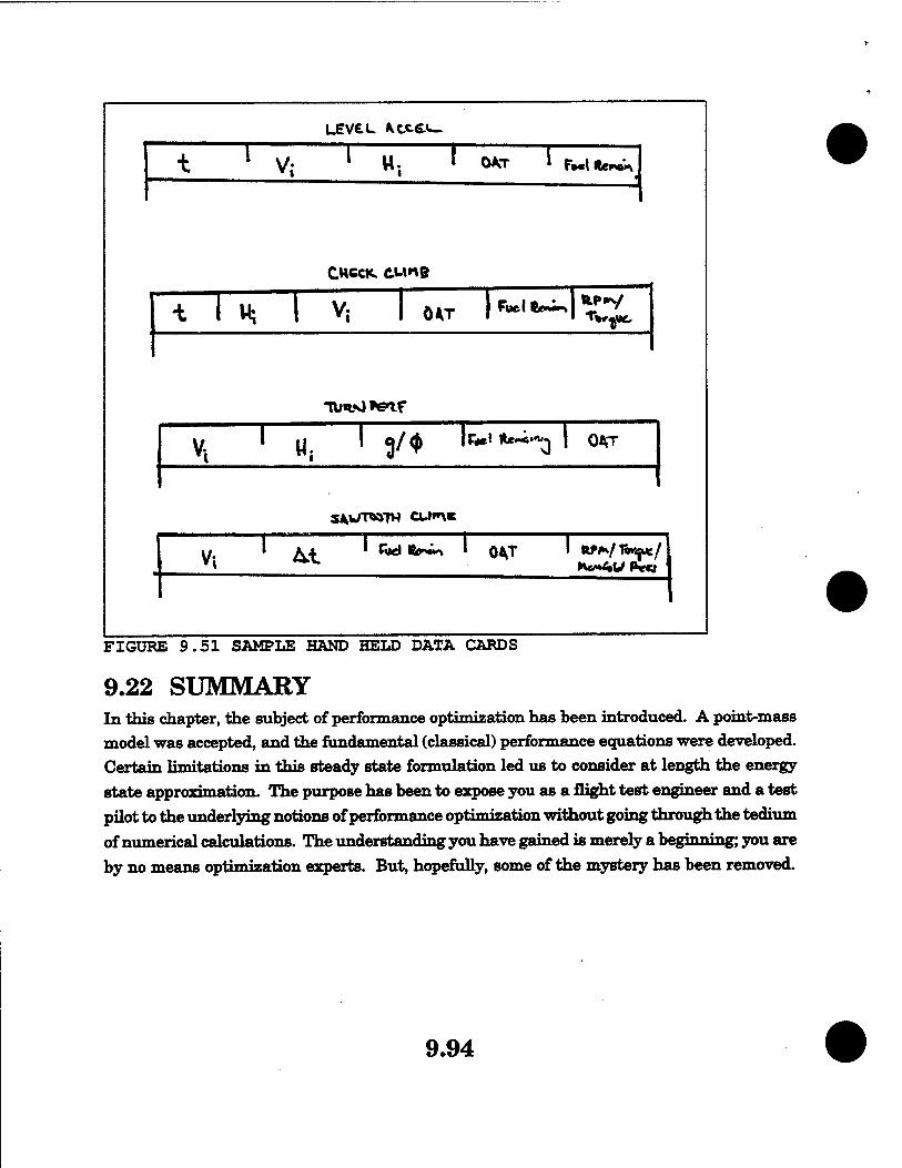
LEVEL KC.C6.I—

t 1 V; ' Hj ' **»• ' Fi.l««wJ

CHccn cun&

* 1 H 1 V, | OKT l*-'«~H^£.

*nm«0*ear

v, 1 u ' 3/$ l***1 ^"O 1 0*T

S^k/TOTW CU»»\«

Vi

FIGÜF \E 9.51 SAMPLE HAND HELD DATA CARDS

9.22 SUMMARY In this chapter, the subject of performance optimization has been introduced. A point-mass model was accepted, and the fundamental (classical) performance equations were developed. Certain limitations in this steady state formulation led us to consider at length the energy state approximation. The purpose has been to expose you as a flight test engineer and a test pilot to the underlying notions of performance optimization without going through the tedium of numerical calculations. The understanding you have gained is merely a beginning; you are by no means optimization experts. But, hopefully, some of the mystery has been removed.

9.94

BIBLIOGRAPHY

91 Bryson, A.E., Jr., Desai, MIL, and Hoffman, W.C., "Energy-State Approbation in Performance Optimization of Supersonic Aircraft," Journal of Aircraft, Vol. 6, No. 6, November-December 1969, pp. 481-488.

9 2 Rutowski, E.S., "Energy Approach to the General Aircraft Performance Problem," Journal of the Aeronautical Sciences, Vol. 21, No. 3, March 1954, pp. 187-195.

9 3 Kelley H.J., and Edelbaum, T.N., "Energy Climbs, Energy Turns, and Asymptotic Expansion," Journal of Aircraft, Vol. 7, No. 1, January-February 1970, pp. 93-95.

9 4 Calise, AJ., "Extended Energy Management Methods for Flight Performance Optimi- zation," AIAA Journal, VoL 15, No. 3, March 1977, pp. 314-321.

9 5 Reaves, G.L., "The Energy Maneuverability Concept and Reconimended Air Combat Tatics for the F-104," The SURE Project, Lecture 6. Lockheed Report CA/ME 2383, July 1967.

9 6 Chase, W.V., "Energy Maneuverability, USAF and USN Aircraft in Clean Configur- ation," APGC-TR-66-4, Vol. H (Part A), Air Force Armament Laboratory, Eghn AFB, FL, December 1966, (SECRET).

9.7 Kelley, H.J., and Lefton, L., "Supersonic Aircraft Energy Turns," Automatica, VoL 8, 1972, pp. 575-580.

9.8 Weir, T.J., "Fundamentals of Air Combat Maneuvering," *-R TWTITIUMII Digest. Vol. 2, No. 5, May 1975, pp. 3-6.

9 9 Olson, W., and Michalik, G., Lt, USAF, "Dynamic Performance Testing on a KC-135/' Presented at 5th Annual Dynamic Performance Workshop, Dryden Flight Research Center, CA, 11-12 May 1982.

9.10 Huckebone, Thomas C, Capt, USAF, and Walker, HenryC L£ Major USAF, p^m^ Evaluation of the X-2QA Research Aircraft. AFFTC-TR-87-51, AFFTC, Edwards AFB, CA March 1988.

9.95