adapting granular materials through artificial evolution · pdf fileresults for simple sphere...

1

Adapting granular materials through artificial evolution

Marc Z. Miskin and Heinrich M. Jaeger

James Franck Institute and Department of Physics, The University of Chicago, Chicago, IL 60637

I. Supplementary Discussion 3-Sphere fitness landscapes for varying friction forces In our simulations, friction is modeled as a linear spring applying load tangentially to the contact between two spheres. The spring constant (kfric) is calibrated to match results for simple sphere packings (set to kcal as detailed in Supplementary Methods). In simulations, we are, however, able to reduce this spring constant in a series of steps to see what kind of a role material parameters play in determining a fitness landscape. For instance, if the spring constant is ramped down to zero from the calibrated value, the landscapes below result.

Fig. S1: Dependence of the 3-sphere fitness landscape on interparticle friction, parameterized by a tangential spring constant, kfric. To best match physical experiments kfric=kcal; this trace corresponds to the data shown in Fig. 1c.

0.4 0.8 1.2 1.60

20

40

60

80

θ (rads)

E you

ng (M

Pa)

Experimental Resultskfric=kcalkfric=kcal/4kfric=kcal/20kfric= 0

SUPPLEMENTARY INFORMATIONDOI: 10.1038/NMAT3543

NATURE MATERIALS | www.nature.com/naturematerials 1

© 2013 Macmillan Publishers Limited. All rights reserved.

http://www.nature.com/doifinder/10.1038/nmat3543

2

As the frictional force vanishes, the fitness landscape transforms from a rugged, complex landscape with definable extrema to being essentially constant within the noise. It is interesting to note that for every setting of the friction coefficient, rods remain the softest particle. These results demonstrate that material parameters play a crucial role in ensuring simulations produce physical results as well as defining what is meant by “optimized.” Deconstruction Proof for Blueprint Rules Blueprint rules can represent any object to the prescribed accuracy of the building blocks. To show this, we demonstrate that any configuration of building blocks can be mapped to at least one blueprint, and thus a blueprint for that object exists. Suppose that we are given a particular configuration of building blocks. We can establish a coordinate system by taking an arbitrary block in the object and designating it as our origin and picking an arbitrary vector in space that we designate as our reference vector. We systematically deconstruct the object by finding the block which is furthest from the origin and removing it. When we remove this block, we also write down the rotations needed to point the reference vector at the site. Last, if two objects are equidistant, simply pick one arbitrarily and then proceed as usual. We continue this process until only the origin remains. It is obvious that these conditions can always be satisfied: there will always be at least one object furthest from the origin, and there will always be a way to point the reference vector at this object. The final list of rotations written down during the deconstruction is, of course, the blueprint in reverse order. By simply traveling along these same vectors and placing spheres instead of removing them the original object could be built back up. Therefore a blueprint can always be constructed for a given object. The crucial ingredient to this process is in specifying that the built spheres are always placed as far as possible from the origin. Using this rule is what makes the list of vectors generated through deconstructing the object the same as the blueprint in reverse order. The rule expresses the notion that, since the order of construction is significant, construction has to proceed in a way that does not prematurely close the building space. As an example, consider building a ring of spheres. The deconstruction is simple to do: pick a sphere at random and designate it as the origin. Then, each sphere is removed according to its distance from the origin, beginning with the sphere diametrically opposed. The list of angles for the removed spheres is the ring blueprint in reverse order. Note that the final sphere closing the ring appears last in the blueprint. If instead of a ring, a disk-like shape were to be produced, all that is required is to change the build order so that this final pair of angles appears instead as the first (following the initial sphere at the

2 NATURE MATERIALS | www.nature.com/naturematerials

SUPPLEMENTARY INFORMATION DOI: 10.1038/NMAT3543



3

origin). Yet if the build rule were, for instance, to place the spheres as close as possible to the origin, the center would always be filled and a ring would be impossible to make. In other words, the "closest placement" build rule prematurely closes the build space, excluding the ring as a build-able object. Transforming the most compact shapes to the stiffest The figure below indicates the motif that allows for constructing the shape that produces the stiffest packing for a given number n of spheres.

Fig. S2: Removing one sphere from the most compact shape for n+1 spheres (left column) produces shapes of n spheres (center) almost identical to those located independently by our algorithm (right column). It is, however, unknown which sphere should be removed to generate the stiffest packing.

Evolutionary Algorithm and Benchmark Tests of Blueprint Rules To test and refine our algorithm, we used it to evolve shapes with known geometric properties. Specifically, we wanted to be sure that our algorithm was able to build different





4

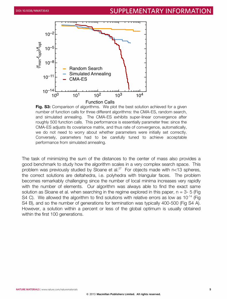
topologies and identify families of shapes. These features also needed to scale well with the number of elements involved in the search problem. In this work, we used evolution strategies (ES) as our primary optimizer due to their emphasis on direct manipulation of real-valued parameters through mutation. Specifically, we chose to use the Covariance Matrix Adaptation Evolution Strategy or CMA-ES developed by Hansen et al.,19 modified to use rank-µ update only. Like most evolution strategies, this algorithm attempts to improve the quality of solutions by examining random perturbations around a given mean solution. The CMA-ES draws these guesses using a multivariate Gaussian distribution. The key feature of this algorithm is that it uses information from prior iterations of the search to deterministically update the mean and covariance matrix. Specifically, the mean of the distribution is updated so that the likelihood of drawing a previously found good candidate is maximized whereas the covariance matrix is updated so as to increase the probability of a successful step. One modification to the fitness metric was included to improve the overall performance of the algorithm. It arises from the fact that the search domain is periodic. Consequently, there are an infinite number of degenerate solutions to a given optimization problem spread out over all of search space. In order to prevent searches from wasting function calls exploring this degeneracy, we included a small multiplicative factor to the fitness values. It rescales the fitness value to increase quadratically if the maximum absolute value of an angle in a blueprint is over π. In that way, the search space is softly bounded and prevented from investigating redundant angles. In comparing our algorithm to other optimization techniques, we found that the CMA-ES outperformed alternatives by requiring significantly fewer function calls to identify a solution. For instance, consider figure S3 which compares the performance of the CMA-ES to simulated annealing and random search. Here, all three algorithms are being used to construct tetrahedrons by minimizing the sum of the distances to the center of mass for 4 spheres. We plot the relative difference between the best solution found and the global optimum against the number of iterations required. We find that early on, after about 500 function calls, the CMA-ES begins to dramatically outperform simulated annealing. Since each generation typically uses about 8 function calls, this corresponds to just over 50 generations.





5

Fig. S3: Comparison of algorithms. We plot the best solution achieved for a given number of function calls for three different algorithms: the CMA-ES, random search, and simulated annealing. The CMA-ES exhibits super-linear convergence after roughly 500 function calls. This performance is essentially parameter free: since the CMA-ES adjusts its covariance matrix, and thus rate of convergence, automatically, we do not need to worry about whether parameters were initially set correctly. Conversely, parameters had to be carefully tuned to achieve acceptable performance from simulated annealing.

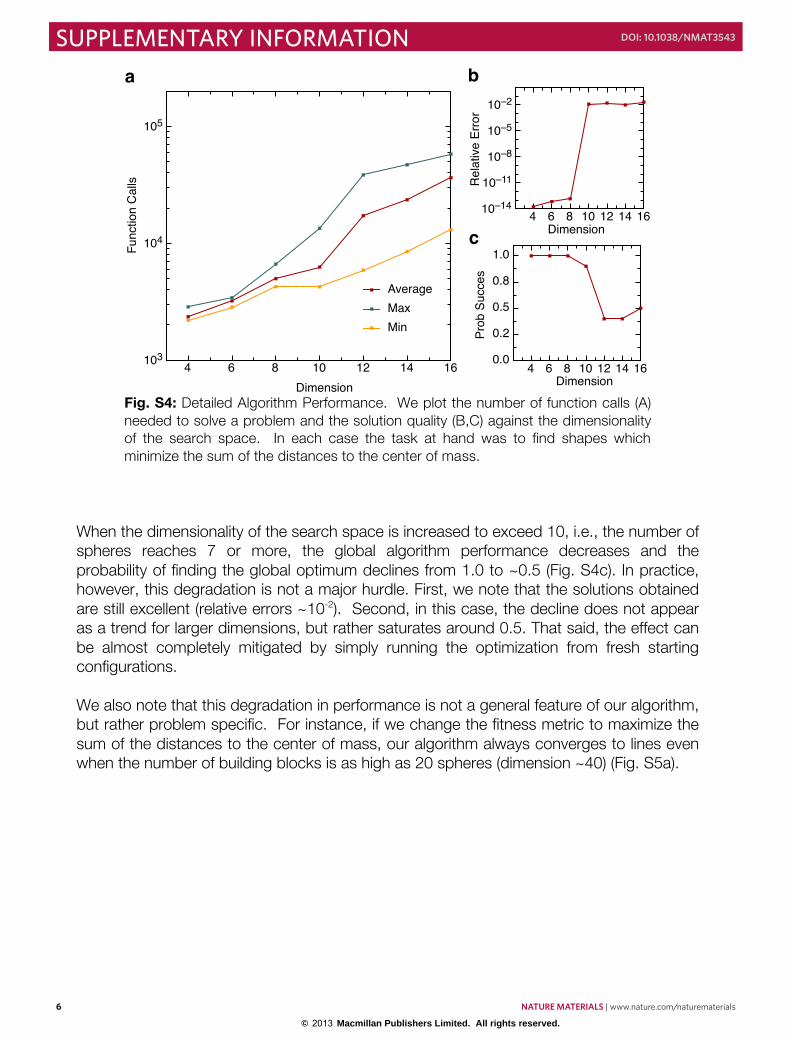
The task of minimizing the sum of the distances to the center of mass also provides a good benchmark to study how the algorithm scales in a very complex search space. This problem was previously studied by Sloane et al.27 For objects made with n<13 spheres, the correct solutions are deltahedra, i.e. polyhedra with triangular faces. The problem becomes remarkably challenging since the number of local minima increases very rapidly with the number of elements. Our algorithm was always able to find the exact same solution as Sloane et al. when searching in the regime explored in this paper, n = 3- 5 (Fig S4 C). We allowed the algorithm to find solutions with relative errors as low as 10-14 (Fig S4 B), and so the number of generations for termination was typically 400-500 (Fig S4 A). However, a solution within a percent or less of the global optimum is usually obtained within the first 100 generations.

100 101 102 103 10410–14

10–11

10–8

10–5

10–2

Function Calls

(f min

-f opt

)/fop

t

Random SearchSimulated AnnealingCMA-ES





6

Fig. S4: Detailed Algorithm Performance. We plot the number of function calls (A) needed to solve a problem and the solution quality (B,C) against the dimensionality of the search space. In each case the task at hand was to find shapes which minimize the sum of the distances to the center of mass.

When the dimensionality of the search space is increased to exceed 10, i.e., the number of spheres reaches 7 or more, the global algorithm performance decreases and the probability of finding the global optimum declines from 1.0 to ~0.5 (Fig. S4c). In practice, however, this degradation is not a major hurdle. First, we note that the solutions obtained are still excellent (relative errors ~10-2). Second, in this case, the decline does not appear as a trend for larger dimensions, but rather saturates around 0.5. That said, the effect can be almost completely mitigated by simply running the optimization from fresh starting configurations. We also note that this degradation in performance is not a general feature of our algorithm, but rather problem specific. For instance, if we change the fitness metric to maximize the sum of the distances to the center of mass, our algorithm always converges to lines even when the number of building blocks is as high as 20 spheres (dimension ~40) (Fig. S5a).

4 6 8 10 12 14 16103

104

105

Dimension

Func

tion

Cal

ls

AverageMaxMin

Dimension

Rel

ativ

e Er

ror

4 6 8 10 12 14 1610–14

10–11

10–8

10–5

10–2

4 6 8 10 12 14 160.0

0.2

0.5

0.8

1.0

Dimension

Prob

Suc

ces

a b

c





7

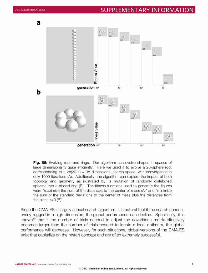
Fig. S5: Evolving rods and rings. Our algorithm can evolve shapes in spaces of large dimensionality quite efficiently. Here we used it to evolve a 20-sphere rod, corresponding to a 2x(20-1) = 38 dimensional search space, with convergence in only 1000 iterations (A). Additionally, the algorithm can explore the impact of both topology and geometry as illustrated by its mutation of randomly distributed spheres into a closed ring (B). The fitness functions used to generate the figures were "maximize the sum of the distances to the center of mass (A)" and "minimize the sum of the standard deviations to the center of mass plus the distances from the plane z=0 (B)".

Since the CMA-ES is largely a local search algorithm, it is natural that if the search space is overly rugged in a high dimension, the global performance can decline. Specifically, it is known19 that if the number of trials needed to adjust the covariance matrix effectively becomes larger than the number of trials needed to locate a local optimum, the global performance will decrease. However, for such situations, global versions of the CMA-ES exist that capitalize on the restart concept and are often extremely successful.





8

For the purpose of the present paper, which aims to provide proof of principle to the power of evolutionary computation applied to granular design, we felt that such refinements were not critical. In particular, our primary limitation did not come from the evolutionary algorithm, but rather from our ability to complete rapid, accurate molecular dynamics (MD) simulations with the computer resources at hand. This issue arises from the complexities of calculating slight relative movements among multi-sphere, bonded compound particles inside a dense, jammed 3D packing. We performed all simulations with a desktop, 16-processor MacPro. Using this basic computer, a complete optimization, which encompass roughly 600 calculations of the stress-strain curve for packings of 2,000 compound particles at each trial, could be completed on practical timescales (roughly 3-7 days) when n<8. Finally, to be sure our algorithm can explore different topologies, we used the code to construct rings from 5 spheres. Again, the code is able to adapt a jumbled mess to a ring in roughly 1000 generations (Fig S5b). Ultimately, compact polyhedra, lines and rings are all equally accessible in our chosen building representation and can be discovered easily by our chosen algorithm. Testing a suboptimal shape To strengthen the claim that our simulations faithfully reproduce the physical fitness landscape, we decided to print one suboptimal shape discovered during the n=4 softest optimization. This shape was discovered shortly before the algorithm began to converge on linear molecules, and thus it is roughly linear but with a slight bend. As noted in the main text, this shape was predicted by the simulation to have a modulus of 46MPa. Experimental packings of 3D-printed copies of such particles were measured to have a modulus of 47 ±1 MPa, in excellent agreement. In the plot below we show the stress strain curves for experimental packings of the stiffest, the softest and the suboptimal particle shape. Clearly the data for the suboptimal shape has a slope, near zero strain, that lies in between the slopes for the two optimal packings. We plot in the inset a comparison between the experimental stress strain curve and the simulated one. Again, the agreement in the region actually considered by our optimizations (i.e. near zero strain) is quite good.





9

Fig. S6: Experimental results for a particle deemed suboptimal by our algorithm (light blue) compared to the experimental results for the stiffest (red) and softest (blue) packing particles. The particles are sketched in the boxes to the right of the main panel. Inset: For the suboptimal shape, comparison of stress strain curves from simulation (dark blue line) and experiment (light blue) near zero strain.

II. Supplementary Methods Calibrating the Simulations and Triaxial Testing Procedure An essential component to our methodology lies in matching the fitness landscape from actual, physical experiments to the surrogate landscape generated by simulations. To achieve this, we established a methodology for generating reproducible triaxial test results, replicated it as closely as possible in the simulation procedure, and calibrated simulation parameters to measured physical parameters. In soil mechanics, its well known that the measured mechanical response of a granular material depends strongly on the loading history and initial state. The intuitive explanation





10

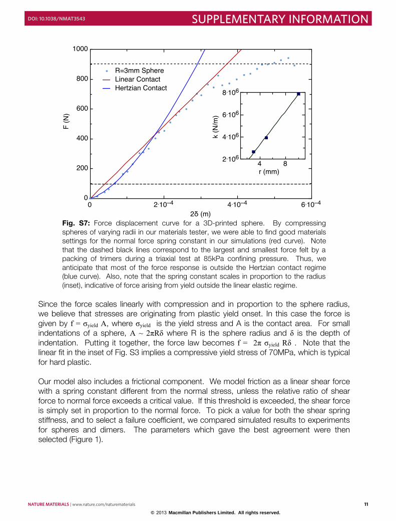
is that a sample of sand packed loosely will behave differently than a sample which had been compacted prior to compression. To establish a reproducible initial state we adopted the following loading and pre-compression procedure for all of our triaxial tests. First, the sample is poured into a latex membrane 50mm in diameter, 130mm tall, 6mm thick, capped on one end. The large aspect ratio is chosen here to decrease the relevance of friction with the end caps. Next, the sample is sealed on the top, and tapped. We lightly tap ~50 times, invert the sample, and then tap 50 more times. The sample is then loaded into an Instron materials tester. The tester holds both the top and bottom caps fixed in place, measuring the force needed to do so. We then pull a vacuum (typically 85kPa) inside the sample to generate confining stress. The top plate is used to compress the sample until the stress on the top plate matches the confining stress. We check to make sure the measured stress is stable for at least 5 seconds, and then begin the compression test. If the stress is seen to fluctuate over this time, we decompress the sample slightly and then press back down until the stresses on all axes are matched again. During compression, samples are compressed at a rate of 10mm/min to strains near 4%. Since the deformation is relatively small, both stress and strain are calculated using the engineering conventions: we divide the measured force/displacement by the initial sample area/length to find the stress/strain values. On the computer we simulate this procedure as closely as possible, using the Pfc3D molecular dynamics software package from Itasca. Isotropic random packings are generated via the radius expansion method. The packings are confined by cylindrical walls. To impose a specific stress state the walls of the cylinder are expanded and contracted, until the desired stress state is reached and stable. The compression test then begins at the same rate as in the experiments. During the test, the top and bottom plates are forced to reach specific values, whereas the cylindrical confining wall is allow to expand or contract such that the packing is always maintained in a quasi-static state. In our experiments using 3D-printed particles, we found that the force can be well approximated as linear in our operating regime, and that the effective spring constant scaled in proportion to the sphere radius. Thus, normal forces between the spheres were modeled as linear contacts. The value for the normal force spring constant was selected by 3D-printed spheres of different radii, compressing them until failure, and measuring force vs displacement (Figure S7). These spheres as well as all other particles used in the experiments discussed in this paper were fabricated with an Objet 350 3D-printer using Vero White or Vero Black UV-curable polymer.





11

Fig. S7: Force displacement curve for a 3D-printed sphere. By compressing spheres of varying radii in our materials tester, we were able to find good materials settings for the normal force spring constant in our simulations (red curve). Note that the dashed black lines correspond to the largest and smallest force felt by a packing of trimers during a triaxial test at 85kPa confining pressure. Thus, we anticipate that most of the force response is outside the Hertzian contact regime (blue curve). Also, note that the spring constant scales in proportion to the radius (inset), indicative of force arising from yield outside the linear elastic regime.

Since the force scales linearly with compression and in proportion to the sphere radius, we believe that stresses are originating from plastic yield onset. In this case the force is given by f = σyield A, where σyield is the yield stress and A is the contact area. For small indentations of a sphere, A ~ 2πRδ where R is the sphere radius and δ is the depth of indentation. Putting it together, the force law becomes f = 2π σyield Rδ . Note that the linear fit in the inset of Fig. S3 implies a compressive yield stress of 70MPa, which is typical for hard plastic. Our model also includes a frictional component. We model friction as a linear shear force with a spring constant different from the normal stress, unless the relative ratio of shear force to normal force exceeds a critical value. If this threshold is exceeded, the shear force is simply set in proportion to the normal force. To pick a value for both the shear spring stiffness, and to select a failure coefficient, we compared simulated results to experiments for spheres and dimers. The parameters which gave the best agreement were then selected (Figure 1).

0 2.10–4 4.10–4 6.10–40

200

400

600

800

1000

2δ (m)

F (N

)R=3mm SphereLinear ContactHertzian Contact

4 82.106

4.106

6.106

8.106

r (mm)

k (N

/m)





12

This procedure works well for two reasons. First, the order of magnitude for the shear spring constant has been set already by selecting the normal spring constant from experimental data. Because of this, the range of parameters for calibration has been dramatically reduced. Second, the shear stiffness value, by definition, plays little to no role in the final yield state. Instead the critical state is largely determined by the friction coefficient. Thus the parameters are effectively orthogonal, allowing the adjustment of one independent of the other. Finally, we note that the agreement between experiment and simulation will degrade if the strain is large. In this case, the change in area of the sample becomes significant and two sources of error arise. First, the use of engineering stress becomes inappropriate, leading to a systematic overestimate in measured stress values. Second, since the simulations constrain the confining wall to remain cylindrical, inhomogeneous deformations of the boundary will result in discrepancy. We ignored these effects in our work since we operate in the low strain regime; however, future studies, in particular those interested in optimizing failure stress, will have to account for these problems explicitly.

Material Parameter Calibrated Value

compressive modulus 70 MPa

density 1,200 kg/m3

normal to shear stiffness 5

friction coefficient 0.25





adapting granular materials through artificial evolution · pdf fileresults for simple sphere...

Documents