Adaptive Aggregation of Markov Chains:Quantitative Analysis of Chemical Reaction Networks ?

Alessandro Abate1, Lubos Brim2, Milan Ceska1,2, and Marta Kwiatkowska1

1 Department of Computer Science, University of Oxford, UK2 Faculty of Informatics, Masaryk University, Czech Republic

Abstract. Quantitative analysis of Markov models typically proceeds throughnumerical methods or simulation-based evaluation. Since the state space of themodels can often be large, exact or approximate state aggregation methods (suchas lumping or bisimulation reduction) have been proposed to improve the scala-bility of the numerical schemes. However, none of the existing numerical tech-niques provides general, explicit bounds on the approximation error, a problemparticularly relevant when the level of accuracy affects the soundness of verifica-tion results. We propose a novel numerical approach that combines the strengthsof aggregation techniques (state-space reduction) with those of simulation-basedapproaches (automatic updates that adapt to the process dynamics). The key ad-vantage of our scheme is that it provides rigorous precision guarantees underdifferent measures. The new approach, which can be used in conjunction withtime uniformisation techniques, is evaluated on two models of chemical reac-tion networks, a signalling pathway and a prokaryotic gene expression network:it demonstrates marked improvement in accuracy without performance degrada-tion, particularly when compared to known state-space truncation techniques.

1 Introduction

Markov models are widely used in many areas of science and engineering in orderto evaluate the probability of certain events of interest. Quantitative analysis of time-bounded properties of Markov models typically proceeds through numerical analysis,via solution of equations yielding the probability of the system residing in a givenstate at a given time, or via simulation-based exploration of its execution paths. Forcontinuous-time Markov chains (CTMCs), a commonly employed method is uniformi-sation (also known as Jensen’s method), which is based on the discretisation of theoriginal CTMC and on the numerical computation of transient probabilities (that is,probability distributions over time). This can be combined with graph-theoretic tech-niques for probabilistic model checking against temporal logic properties [4].

There are many situations where highly accurate probability estimates are neces-sary, for example for reliability analysis in safety-critical systems or for predictivemodelling in scientific experiments, but this is difficult to achieve in practice because

? This work has been partially supported by the ERC Advanced Grant VERIWARE, the CzechMinistry of Education, Youth, and Sport project No. CZ.1.07/2.3.00/30.0009 (M. Ceska), theCzech Grant Agency grant No. GA15-11089S (L. Brim), the John Fell Oxford University Press(OUP) Research Fund, and by the European Commission IAPP project AMBI 324432.

of the state-space explosion problem. Imprecise values are known to lead to lack ofrobustness, in the sense that the satisfaction of temporal logic formulae can be affectedby small changes to the formula bound or the probability distribution of the model.Simulation-based analysis does not suffer from this problem and additionally allowsdynamic adaptation of the sampling procedure, as e.g. in importance sampling, to thecurrent values of the transient probability distribution. However, this analysis providesonly weak precision guarantees in the form of confidence intervals. In order to enablethe handling of larger state spaces, two types of techniques have been introduced: stateaggregation and state-space truncation. State aggregation techniques build a reducedstate space using lumping [6] or bisimulation quotient [21], and have been proposedboth in exact [21] and approximate form [10], with the latter deemed more robust thanthan the exact ones [11]. State-space truncation methods, e.g. fast adaptive uniformisa-tion (FAU) [9,23], on the other hand, only consider the states whose probability mass isnot negligible, while clustering states where the probability is less than a given thresh-old and computing the total probability lost. Unfortunately, though these methods allowthe user to specify a desired precision, none provide explicit and general error boundsthat can be used to quantify the accuracy of the numerical computation: more precisely,these truncation methods provide a lower bound on the probability distributions in time,and the total probability lost can be used to derive a (rather conservative) upper boundon the (point-wise) approximation error as the sum of the lower bound and of the totalprobability lost.

Key contributions We propose a novel adaptive aggregation method for Markov chainsthat allows us to control its approximation error based on explicitly derived error bounds.The method can be combined with numerical techniques such as uniformisation [9,23],typically employed in quantitative verification of Markov chains. The method worksover a finite time interval by clustering the state space of a Markov chain sequentiallyin time, where the quality of the current aggregation is quantified by a number of met-rics. These metrics, in conjunction with user-specified precision requirements, drive theprocess by automatically and adaptively reclustering its state space depending on theexplicit error bounds. In contrast to related simulation-based approaches in the litera-ture [13,31] that employ the current probability distribution of the aggregated model toselectively cluster the regions of the state space containing negligible probability mass,our novel use of the derived error bounds allows far greater accuracy and flexibility asit accounts also for the past history of the probability mass within specific clusters.

To the best of our knowledge, despite recent attempts [10, 11] the development anduse of explicit bounds on the error associated with a clustering procedure is new for thesimulation and analysis of Markov chains. The versatility of the method is further en-hanced by employing a variety of different metrics to assess the approximation quality.More specifically, we use the following to control the error: (1) the probability distribu-tions in time (namely, the point-wise difference between concrete and abstract distribu-tions), (2) the time-wise likelihood of events (L1 norm and total variation distance), aswell as (3) the probability of satisfying a temporal logic specification.

We implement our method in conjunction with uniformisation for the computationof probability distributions of the process in time, as well as time-bounded probabili-ties (a key procedure for probabilistic model checking against temporal logic specifi-

cations), and evaluate it on two case studies of chemical reaction networks. Comparedto fast adaptive uniformisation as implemented in PRISM [9], currently the best per-forming technique in this setting, we demonstrate that our method yields a markedimprovement in numerical precision without degrading its performance.

Related work (Bio-)chemical reaction networks can be naturally analysed using dis-crete stochastic models. Since the discrete state space of these models can be largeor even infinite, a number of numerical approaches have been proposed to alleviatethe associated state-space explosion problem. For biochemical models with large pop-ulations of chemical components, fluid (mean-field) approximation techniques can beapplied [5] and extended to approximate higher-order moments [12]: these determin-istic approximations lead to a set of ordinary differential equations. In [16], a hybridmethod is proposed that captures the dynamics using a discrete stochastic descriptionin the case of small populations and a moment-based deterministic description for largepopulations. An alternative approach assumes that the transient probabilities can becompactly approximated based on quasi product forms [3]. All the mentioned methodsdo not provide explicit accuracy bounds of approximation.

A widely studied model reduction method for Markov models is state aggrega-tion based on lumping [6] or (bi-)simulation equivalence [4], with the latter notion inits exact [21] or approximate [10] form. In particular, approximate notions of equiva-lence have led to new abstraction/refinement techniques for the numerical verificationof Markov models over finite [11] as well as uncountably-infinite state spaces [1,2,26].Related to these techniques, [27] presents an algorithm to approximate probability dis-tributions of a Markov process forward in time, which serves as an inspiration for ouradaptive scheme. From the perspective of simulations, adaptive aggregations are dis-cussed in [13] but no precision error is given: our work differs by developing an adaptiveaggregation scheme, where a formal error analysis steers the adaptation.

An alternative method to deal with large/infinite state spaces is truncation, wherea lower bound on the transient probability distribution of the concrete model is com-puted, and the total probability mass that is lost due to this truncation is quantified.Such methods include finite state projections [24], sliding window abstractions [18],or fast adaptive uniformisation (FAU) [9, 23]. Apart from truncating the state space byneglecting states with insignificant probability mass, FAU dynamically adapts the uni-formisation rate, thus significantly reducing the number of uniformisation steps [30].The efficiency of the truncation techniques depends on the distribution of the signifi-cant part of the probability mass over the states, and may result in poor accuracy if thismass is spread out over a large number of states, or whenever the selected window ofstates does not align with a property of interest.

Summarising, whilst a number of methods have been devised to study or to simulatecomplex biochemical models, in most cases a rigorous error analysis is missing [13,22,31], or the error analysis cannot be effectively used to obtain accurate bounds on theprobability distribution or on the likelihood of events of interest [17].

Structure of this article Section 2 introduces the sequential aggregation approach toapproximate the transient probability distribution (that is, the distribution over time) ofdiscrete-time Markov chains, and quantifies bounds on the introduced error according

to three different metrics. Section 3 applies the aggregation method for temporal logicverification of Markov chains. In Section 4, we implement adaptive aggregation forcontinuous-time Markov chain models of chemical reaction networks, in conjunctionwith known techniques such as uniformisation and threshold truncation. Finally, Section5 discusses experimental results.

2 Computation of the transient probability distribution

We first work with discrete-time labelled Markov chains (LMC), and in Section 4 weshow how to apply the obtained results to (labelled) continuous-time Markov chains.Formally, an LMC is defined as a triple (S , P, L), where

– S = {s1, . . . , sn} is the finite state space of size n;– P : S × S → [0, 1] is the transition probability matrix, which is such that ∀ j ∈ S :∑n

i=1 P ji =∑n

i=1 P( j, i) = 1;– L : S → 2Σ is a labelling function, where Σ is a finite alphabet built from a set of

atomic propositions.

Whenever clear from the context, we refer to the model simply as (S , P). The model isinitialised via distribution π0 : S → [0, 1],

∑s∈S π0(s) = 1, and its transient probability

distribution at time step k ≥ 0 is

πk+1(s) =∑s′∈S

πk(s′)P(s′, s), (1)

or more concisely as πk+1 = πkP (where the πk’s are row vectors). We are interested inproviding a compact representation and an efficient computation of the vectors πk.

Sequential aggregations of the Markov chain

Consider the finite time interval of interest [0, 1, . . . ,N]. Divide this interval into a givennumber (q) of sub-intervals, namely select N1,N2, . . . ,Nq :

∑qi=1 Ni = N, and consider

the evolution of the model within the corresponding l-th interval [∑l−1

i=0 Ni,∑l

i=0 Ni], forl = 1, . . . q, and where we have set N0 = 0.

We assume that a specific state-space aggregation is given, for each of the q sub-intervals of time. Later, in Section 4, we show how such aggregations can be obtainedadaptively, based on a number of measures (such as the current value of the aggregatedtransient probability distribution, or the accrued aggregation error in time). In partic-ular, at the l-th step (where l = 1, . . . , q), the state space is partitioned (clustered) asS = ∪

mli=1S l

i (consider that the cardinality index ml has been reasonably selected so thatml << n), and denote the abstract (aggregated) state space simply as S l and its ele-ments (the abstract states) with φi, i = 1, . . . ,ml. Introduce abstraction and refinementmaps as αl : S → S l and Al : S l → 2S , respectively – the first takes concrete pointsinto abstract ones, whereas the latter relates abstract states to concrete partitioning sets.For any pair of indices i, j = 1, . . . ,ml, define the abstract transition matrix as

Pl(φ j, φi) �1

| Al(φi) |

∑s∈Al(φi)

∑s′∈Al(φ j)

P(s′, s).

The intuition behind the aggregated matrix Pl is that it encompasses the average in-coming probability from clusters S j to S i. The shape of this matrix is justified by thestructure of the update equation in (1). Given the aggregated Markov chain, we shallwork, for all s ∈ S l, with the following recursions:

πlk+1(s) =

∑s′∈S 1

πlk(s′)Pl(s′, s).

The smaller, aggregated model (S l, Pl) serves as basis for an approximate computationof the transient probability in time: we now calculate an explicit upper bound on the ap-proximation error. In order to quantify this error, we define a function ε l : [1, . . . ,ml]2 →

[0, 1], as follows:

ε l( j, i) � maxs∈S l

i

∣∣∣∣∣∣∣ | Sli |

| S lj |

P(S j, s) − Pl(φ j, φi)

∣∣∣∣∣∣∣ . (2)

Intuitively, this quantity accounts for the difference between the average incoming prob-ability between a pair ( j, i) of partitioning sets, and the worst-case (rescaled) point-wiseincoming probability between those two sets. Introduce the terms ε l( j) :=

∑mli=1 ε

l( j, i).Finally, define, for all s ∈ S , πl

k(s) = πlk(αl(s))/ | Al(αl(s)) | as a (normalised)

piecewise constant approximation of the abstract functions πlk. Functions πl

k, being de-fined over the concrete state space S , will be employed for comparison with the originaldistribution functions πk. Specifically, for the initial interval [N0,N1] (with l = 1), ap-proximate the initial distribution π0 by π1

0 as: ∀s ∈ S 1, π10(s) =

∑s′∈A1(s) π0(s′). Similarly,

we have that ∀s ∈ S , π10(s) = π1

0(α1(s))/ | A1(α1(s)) |.

Remark 1. Exact and approximate probabilistic bisimulations [10, 21] build a quotientor a cover of the state space of the original model based on matching or approximatingthe “outgoing probability” from concrete states – for example, exact probabilistic bisim-ulation compares, for state pairs (s1, s2) within a partition, the “outgoing” probabilitiesP(s1, B) and P(s2, B) over partitions B. On the other hand, in (2) we approximate the“incoming probability”, as motivated by the approximation of the recursions in (1). ut

Explicit error bounds for the quality of the sequential aggregations

Let us consider the aggregated model (S 1, P1) (for l = 1) and, given the aggregated vec-tor π1

0, the time-wise updates π1k+1 = π1

k P1, k = N0, . . . ,N1−1. Introduce the interpolatedvectors π1

k+1(s), s ∈ S , defined as π1k+1(s) = π1

k+1(α1(s))/ | A1(α1(s)) |. We are inter-ested in a bound on the point-wise error defined over the concrete state space, namely∀s ∈ S , k = N0, . . . ,N1,

∣∣∣πk(s) − π1k(s)

∣∣∣, or equivalently a bound for∣∣∣∣πk(s) − π1

k (α1(s))|A1(α1(s))|

∣∣∣∣.Such a point-wise bound directly allows for expressing a global error for the infinitynorm of the difference between the two distribution vectors, namely∥∥∥πk − π

1k

∥∥∥∞

= maxs∈S

∣∣∣πk(s) − π1k(s)

∣∣∣ .Beyond the first aggregation (l = 1), the next statement explicitly characterises such abound over the entire sequence of q re-aggregations and the time interval [0, 1, . . . ,N].

Proposition 1. Consider a sequential q-step aggregation strategy, characterised bytimes Nl :

∑ql=1 Nl = N, partitions S = ∪

mli=1S l

i, and matrices Pl. We obtain∣∣∣πN(s) − πqN(s)

∣∣∣ ≤ c(s)N∣∣∣π0(s) − π1

0(s)∣∣∣

+

q∑l=1

c(s)N−∑l

i=0 Ni

1| Al(αl(s)) |

ml∑j=1

ε l( j, αl(s))Nl−1∑k=0

πl∑l−1i=0 Ni+k

( j) + γll−1(s)

,where we have set c(s) = P(S , s), and where γl

l−1(s) =

∣∣∣∣∣πl−1∑l−1i=0 Ni

(s) − πl∑l−1i=0 Ni

(s)∣∣∣∣∣ for

l = 1, . . . , q, with γ10(s) = 0, ∀s ∈ S .

Remark 2. A few comments on the structure of the error bounds are in order. Theoverall error is composed of two main contributions, one depending on the error ac-crued within single aggregation steps, and the other (γl

l−1(s)) depending on the q re-aggregations (that is, an update from the current partition to the next).

The first term of the first contribution further depends on the point-wise error in

the distributions initialised at each aggregation, namely,∣∣∣∣∣π∑l

i=0 Ni(s) − πl∑l

i=0 Ni(s)

∣∣∣∣∣: this

quantity, discounted by the Nl-th power of the factor c(s) (accounting for contractive orexpansive dynamics), builds up recursively to yield the global (over the q aggregationsteps) quantity c(s)N

∣∣∣π0(s) − π10(s)

∣∣∣. The second term of the first contribution, on theother hand, accounts for the error due to the approximation of the transition probabilitymatrix (terms ε l), averaged over the accrued running distribution functions (factors πl).

The intuition on factor c(s) is the following: if the model is “contractive” (in acertain probabilistic sense) towards a point s, the factor c(s) is likely to be greater thanone; on the other hand, if the distribution in time is “dispersed,” then it is likely thatc(s) < 1 over a large subset of the state space. The quantity c(s) = P(S , s) might bedecreased if we work on a subset of S : this might happen with a discrete-time chainobtained from a corresponding continuous-time model via FAU [9, 23], or through theinteraction of the factor c(s), s ∈ S , with atomic propositions defined specifically oversubsets of the state space S . ut

Corollary 1. Consider the same setup as in Proposition 1. A bound for the quantity∥∥∥πN − πqN

∥∥∥∞

can be obtained from that in Proposition 1 by straightforward adaptationand setting c = maxs∈S c(s), and γl

l−1 = maxs∈S γll−1(s), l = 1, . . . , q.

In addition to point-wise errors, we seek a bound for the following global error,∥∥∥πk − π1k

∥∥∥1 =

∑s∈S

∣∣∣πk(s) − π1k(s)

∣∣∣ , ∀k = 0, . . . ,N1,

and its further extension to successive aggregations and time steps k = N1 + 1, . . . ,N.This L1-norm measure is related to the “total variation distance” over events in theσ-algebra 2S at each time step k. This measure is commonly used in related litera-ture [8, 29], and refers to differences in probability of events defined over sets in Sat a specific point in time k. The corresponding error bound is explicitly quantified asfollows.

Proposition 2. Consider a q-step sequential aggregation strategy characterised by thetimes Nl :

∑ql=1 Nl = N, partitions S = ∪

mli=1S l

i, and matrices Pl. We obtain

∥∥∥πN − πqN

∥∥∥1 ≤

∥∥∥π0 − π10

∥∥∥1 +

q∑l=1

ml∑j=1

ε l( j)Nl−1∑k=0

πl∑l−1i=0 Ni+k

( j) + Γll−1

,where for l = 1, . . . , q, Γl

l−1 =

∥∥∥∥∥πl−1∑l−1i=0 Ni− πl∑l−1

i=0 Ni

∥∥∥∥∥1, and where we have set Γ1

0 = 0.

3 Aggregations for model checking of time-bounded specifications

In Section 2, we have introduced a sequential aggregation procedure to approximatethe computation of the transient probability distribution of a Markov chain. The derivedbounds allow for a comparison of aggregated and concrete models either point-wise,or according to a global measure of the differences in the probability of events overthe state space, at a specific point in time. We now show how to employ the aggrega-tion method for quantitative verification against probabilistic temporal logics such asPCTL. We focus on a bounded variant of the probabilistic safety (invariance) property,which corresponds to time-bounded invariance for continuous-time Markov chains (tobe studied in Section 4).

Consider the LMP (S , P, L). We focus on properties expressed over the atomicpropositions AP, namely the set of finite strings over the labels 2AP, and on how toapproximately compute the likelihood associated to such strings. In particular, considera step-bounded safety formula [4], namely P=?

(G≤NΦ

), where N ∈ N, and Φ ∈ 2Σ ,

Sat(Φ) ⊆ S 3. This specification expresses the likelihood that a trajectory, initialised ac-cording to a distribution (say, π0) over the state space S , resides within set Φ over thetime interval [0, 1, . . . ,N]. The specification of interest can be characterised as follows:for any s ∈ S , k = 0, 1, . . . ,N − 1,

V0(s) = 1Φ(s)π0(s), Vk+1(s) = 1Φ(s)∑s′∈S

Vk(s′)P(s′, s),

so that P=?

(G≤NΦ

)=

∑s∈S VN(s). It is well known that the computed quantity depends

on the choice of the initial distribution π0 (which can in particular be a point mass for adistinguished initial state). As should be clear from the recursion above (use of indicatorfunctions 1Φ), it is sufficient to restrict the recursive updates to within the set of pointslabelled by Φ.

As before, consider the global finite interval [0, 1, . . . ,N], and divide it via intervalsof duration N1,N2, . . . ,Nq :

∑qi=1 Ni = N. Specifically, for the initial interval [N0,N1]

(corresponding to index q = 1), partition set Φ as Φ = ∪m1i=1Φ

1i – notice that the partition

does not cross the boundaries of the setΦ. Thus S 1 = Φ1∪{a1} = {1, . . . ,m1, a1}, wherea1 is associated with the complement set S \ Φ. Introduce abstraction and refinement

3 For the sake of simplicity, we shall often loosely identify the set Sat(Φ) with label Φ.

maps as α1 : S → S 1 and A1 : S 1 → 2S , the abstract transition matrix P1, and functionε1 : [1, . . . ,m1]2 → [0, 1] as

ε1( j, i) � maxs∈Φ1

i

∣∣∣∣∣∣∣ | Φ1i |

| Φ1j |

P(Φ1j , s) − P1(φ j, φi)

∣∣∣∣∣∣∣ .Further, approximate π0 as: ∀s ∈ S 1, π1

0(s) =∑

s′∈A1(s) π0(s′). Introduce, ∀s ∈ S 1, costfunctions Vi via the following recursions:

V10 (s) = 1Φ1 (s)π1

0(s), V1k+1(s) = 1Φ1 (s)

∑s′∈S 1

V1k (s′)P1(s′, s),

and, ∀s ∈ S , V1k (s) = V1

k (α1(s))/|A1(α1(s))|, as a (normalised) piecewise constantapproximation of the abstract functions V1

k , and in particular initialised as π10(s) =

π10(α1(s))/|A1(α1(s))|. We shall derive explicit bounds on the computation of the error:∣∣∣∣∣∣∣∑s∈Φ VN1 (s) −

∑s∈Φ

V1N1

(s)

∣∣∣∣∣∣∣ =

∣∣∣∣∣∣∣m1∑i=1

∑s∈Φi

(VN1 (s) − V1

N1(s)

)∣∣∣∣∣∣∣ ,and extend them over successive aggregation and time steps k = N1 + 1, . . . ,N. Noticethat, in this instance, we are comparing two scalars, comprising the likelihoods associ-ated with the specification of interest computed over the concrete and abstract models,respectively. More precisely, in general we have:∣∣∣∣∣∣∣∑s∈Φi

VN1 (s) −∑s∈Φi

V1N1

(s)

∣∣∣∣∣∣∣=∣∣∣∣∣∣∣∑s∈Φi

VN1 (s) −∑s∈Φi

V1N1

(α1(s))

|A1(α1(s))|

∣∣∣∣∣∣∣=∣∣∣∣∣∣∣∑s∈Φi

VN1 (s) − V1N1

(i)

∣∣∣∣∣∣∣ .Proposition 3. Consider a q-step sequential aggregation strategy characterised by cor-responding times Nl :

∑ql=1 Nl = N, partitions Φ = ∪

mli=1Φ

li, and matrices Pl. We obtain:∣∣∣∣∣∣∣∑s∈Φ VN(s) −

∑s∈Φ

VqN(s)

∣∣∣∣∣∣∣ ≤q∑

l=1

ml∑i=1

ε l(i)Nl−1∑k=0

V l∑l−1i=0 Ni+k

(i).

Remark 3. We give some intuition regarding the structure of the bounds. The quantitydepends on a summation over q aggregation steps. It expresses the accrual of the errorincurred over the outgoing probability from the i-th partition (term ε l(i)), averaged overthe history of the cost function over that partition. Note the symmetry between the shapeof the bound and the recursive definition of the quantities of interest. ut

4 Quantitative analysis of chemical reaction networks

A chemical reaction network describes a biochemical system containing M chemicalspecies participating in a number of chemical reactions. The state of a model of thesystem at time t ∈ R+ is the vector X(t) = (X1(t), X2(t), . . . , XM(t)), where Xi denotesthe number of molecules of the i-th species [15]. Whenever a single reaction occurs

the state changes based on the stoichiometry of the corresponding reaction. We use Sto denote the set of (discrete) states. Further, for s ∈ S , πt(s) denotes the probabilityP(X(t) = s). Assuming finite volume and temperature, the model can be interpretedas a continuous-time Markov chain (CTMC) C = (S ,R), where the rate matrix R(s, s′)gives the rate of a transition from states s to s′, and π0 specifies the initial distributionover S . The time evolution of the model is governed by the Chemical Master Equation(CME) [15], namely d

dtπt = πt ·Q, where Q is the infinitesimal generator matrix, definedas Q(s, s′) = R(s, s′) if s , s′, and as 1 −

∑s′′,s R(s, s′′) otherwise. The exact solution

of the CME is in general intractable, which has led to a number of possible numericalapproximations [25]. We employ uniformisation [30], which in many cases outperformsother methods and also provides an arbitrary, user-defined approximation precision.

Uniformisation is based on a time-discretisation of the CTMC. The distribution πt

is obtained as a sum (over index i) of terms giving the probability that i discrete re-action steps occur up to time t: this is a Poisson random variable γi,λ·t = e−λ·t · (λ·t)i

i! ,where the time delay is exponentially distributed with rate λ. More formally, πt =∑∞

i=0 γi,λ·t · π0 · Qi ≈∑N

i=0 γi,λ·t · π0 · Qi, where Q is the uniformised infinitesimal gen-erator matrix defined using terms R(s,s′)

λ, and where the uniformisation constant λ is

equal to the maximal exit rate∑

s′′,s R(s, s′′). Although the sum is in general infinite,for a given precision an upper bound N can be estimated using techniques in [14], whichalso allow for efficient computation of the Poisson probabilities γi,λ·t.

For complex models with very large or possibly infinite state spaces, the abovenumerical approximations are computationally infeasible, and are typically combinedwith (dynamical) state-space truncation methods, such as finite state projection [24],sliding window abstraction [18], or fast adaptive uniformisation [9,23] (FAU). The keyidea of these truncation methods is to restrict the analysis of the model to a subset ofstates containing significant probability mass. One can easily compute the probabilitylost at each uniformisation step and thus obtain the total probability lost by truncation.As such, these truncation methods provide a lower bound on the quantities πt, and thequantified probability lost can be used to derive a (rather conservative) upper bound onthe approximation error: the sum of the lower bound and the probability lost gives anupper bound for the point-wise error. Moreover, a (pessimistic) bound on the L1-normover a general subset of the state space is obtained by multiplying the probability lostby the number of states in the concrete subset.

Adaptive aggregation for CTMC models of chemical reaction networks

The aggregation methods in the previous sections can be directly applied to uniformisedCTMCs, such as those arising from chemical reaction networks. We now discuss howthe aggregation unfolds sequentially in time and how the derived error bounds can beused for the aggregation method in this setting.

Recall from eq. (2) that the derivation of the error bounds for the aggregation proce-dure requires a finite state space: for infinite-state CTMCs, the aggregation method canbe combined with state-space truncation (alongside time uniformisation), in order toaccelerate computations in cases where the set of significant states is still too large. Onthe other hand, for finite-state CTMC models, adaptive aggregations can be regardedas an orthogonal strategy to truncation, and can be directly applied in conjunction with

time uniformisation. In order to compare the precision and reduction capability of ourmethod to that of FAU, we thus assume that the population of each species is bounded,which ensures fairness of experimental evaluation.

Algorithm 1 Adaptive aggregation scheme for computation of transient probabilityRequire: Finite CTMC C = (S ,R), initial distribution π0, time t, and bound θ on L1-norm errorEnsure: globalError ≤ θ1: (P,N)← uniformise (C, t) ; l← 12:

(S l, Pl, πl

0, εl)← initAggregation (S , P, π0)

3: for (k ← 0; k ≤ N, k ← k + 1) do . perform N uniformisation steps4: (globalError, AccumErrors)← computeErrors

(πl

k, εl, k

)5: πl

k+1(s) =∑

s′∈S 1 π1k(s′)Pl(s′, s) . update the probability distribution

6: if checkAggregation(ε l, πl

k+1, AccumErrors, θ)

= false then7: (S l+1, Pl+1, πl+1

k+1, εl+1)← Recluster

(S l, Pl, πl

k+1, εl, AccumErrors

)8: AccumErrors← 0; l← l + 1

The key ingredient of the proposed aggregation method is a partitioning strategythat controls and adapts the clustering of the state space over the given finite time in-terval. Algorithm 1 summarises the scheme for transient probability calculation (theadaptive aggregation for an invariant property as in Section 3 unfolds similarly). Theprocedure starts with a given partition S 1 of the state space S (obtained by the proce-dure initAggregation on line 2). It dynamically (and automatically) updates the currentpartition when needed, thus providing new abstract state spaces S l over the l-th timeinterval [

∑l−1i=0 Ni,

∑li=0 Ni], where l = 2, . . . , q and q << N. The update of the current

l-th clustering is performed after Nl steps, that is, whenever the error accrual exceedsa threshold ensuring the user-defined precision θ (function checkAggregation on line6). At the same time, the aggregation strategy aims to minimise the average size of theabstract state space, defined as avg =

∑ql=0 Nl · |S l|/N. We consider two adaptive strate-

gies, one time-local and the other history-dependent, both of which are driven by theshape of the derived error bounds – in particular, the history-dependent strategy exactlyemploys the calculated error bounds. Both strategies are parametrised by thresholds,which ensure the required overall precision θ and account for the size of the concretestate space as well as the number of uniformisation steps N.

The history-dependent strategy is based on the available history contributing tothe shape of the derived errors: for the l-th aggregation step and the given i-th clus-ter of the current partition, it tracks the sum of the errors accumulated in the interval[∑l−1

i=0 Ni,∑l−1

i=0 Ni + k] for k = 1, . . . ,Nl, according to the explicit bounds derived in Sec-tion 2 (line 4 of Algorithm 1). At each step k, the obtained value (averaged over k steps)reflects the (averaged) error accrual for each cluster (array AccumErrors) and is usedto drive the partitioning procedure.

The function checkAggregation determines (using AccumErrors) if the currentclustering meets the desired threshold, or if a refinement is desirable: during re-cluster-ing, a locally coarser abstraction may as well be suggested by merging clusters. Thefunction Recluster provides the new clustering based on the error bounds, which arefunctions of AccumErrors, of the local contributions ε l, and of the (history of the) dis-tribution πl

k (or of the cost V lk in the case of safety verification). In contrast to the adap-

tive method presented in [13] and based exclusively on local heuristics, our strategyclosely reflects the shape of the derived, history-dependent error bounds. Note that theaggregation strategy applied to chemical reaction networks aligns well with the knownstructure of the underlying CTMCs. In particular, the state-space clustering employsthe spatial locality of the distribution of transitions in the M-dimensional space [13,31](M is the number of chemical species), usually leading to relatively uniform probabilitymass over adjacent states and thus to strategies that cluster neighbouring states.

A simpler re-clustering strategy (denoted in the experiments as local) employs ateach uniformisation step k only the product of the local error ε l with the probabilitydistribution πl

k (or with the cost function V lk). In other words, a local re-clustering is

performed if the local error depending on ε lπlk (respectively, on ε lV l

k) is above a giventhreshold. This intuitive scheme is similar to the local heuristic employed in [13].

We will show that the history-based strategy is more flexible with respect to therequired precision and aggregation size. Our experiments confirm that, while based onerror bounds that over-estimate the actual empirical error incurred in the aggregation,the history-based strategy tends to outperform the more intuitive and easier local strat-egy, with respect to key performance metrics affecting the practical use of the adaptiveaggregation. This shows that the computed errors not only serve as a means to certifythe accuracy of approximation, but can also be used to effectively drive the aggrega-tion procedure. In particular, the metrics we are interested in are: (1) the value of avgrepresenting the state-space reduction; (2) the accuracy of the empirical results of theabstract model; (3) the total number of re-clusterings; and (4) the actual value of theerror bounds (compared to the empirical errors).

The number of re-clusterings (denoted by q) is crucial for the performance of theoverall scheme, since each re-clustering requires O(|S | + |P|) steps, which is similar toperforming a few uniformisation steps for the concrete model. As such, the number ofre-clusterings should be significantly smaller than the total number of uniformisationsteps. Therefore, in our experiments we use thresholds that favour fewer re-clusteringsover coarser abstractions. Finally, note that the adaptive aggregation scheme can becombined with the adaptive uniformisation step as well as with dynamic state-spacetruncation [9, 23, 30], which updates the uniformisation constant λ for different timeintervals, thus decreasing the number of overall uniformisation steps N.

Illustrative example We resort to a two-dimensional discrete Lotka-Volterra “predator-prey” model [15] to illustrate the history-dependent aggregation strategy. The maximalpopulation of each species is bounded by 2000, thus the concrete model has 4M states.The initial population is set to 200 predators and 400 preys.

Figure 1 displays the outcome of the adaptive procedure (top row) at three distincttime steps and (bottom row) the current probability distribution of the concrete model.For ease of visualisation, the top plots display for each point of the concrete model thesize of its corresponding cluster, where we have limited the maximal size to 100 states.Note the close correspondence between the error bounds and the computed empiricalerrors, and the limited number of re-clusterings needed (one in about 200 uniformisationsteps). Observe that the single-state clusters (red colour in the plots) tend to collectwhere the current probability distribution peaks. The figure also illustrates a memoryeffect due to the history-dependent error bounds employed by the aggregation.

1

100

50C

lust

er

size

112K

t=0.05 (5K unif. steps) t=0.1 (10K unif. steps) t=0.2 (20K unif. steps)

Prob

abili

ty m

ass

1E-5

0

1E-20

Prey

(0,0)

218K 350K

(2K,2K)

Pre

dato

r

Number of states:Epirical L1 norm:

Re-clusterings:Formal bounds: 5.94E-6

3.27E-71.41E-71.18E-5

6.82E-72.24E-5

27 56 81

Fig. 1. Transient analysis of the Lotka-Volterra model using history-based adaptive aggregation.

5 Experimental evaluation on two case studies

We have developed a prototype implementation of the adaptive aggregation for thequantitative analysis of chemical reaction networks modelled in PRISM [20]. We haveevaluated the scheme on two case studies in comparison with FAU [9] as implementedin the explicit engine of PRISM. In order to ensure comparability between the twoschemes, which employ different data structures, rather than measuring execution timewe have focused on assessing performance based on measures that are independentof implementation, and specifically focused on the metrics (1)-(4) introduced in Sec-tion 4 (model reduction, empirical accuracy, number of re-clusterings, and formal errorbounds). For the same reason, we have not incorporated heuristics such as varying themaximal cluster size, optimally selecting error thresholds, or use of advanced clusteringmethods, which can be employed to further optimise the adaptive scheme.

We run all experiments on a MackBook AirTM

with 1.8GHz Intel Core i5 and 4 GB1600 MHz RAM. As expected, for comparable state space reductions (value avg), FAUcan be faster but in the same order of magnitude as our prototype, due to the overhead ofclustering and adaptive uniformisation not being fully integrated in our implementation.

Recall that FAU eliminates states with incoming probability lower than a definedthreshold, and as such leads to an under-approximation of the concrete probability dis-tribution with no tailored error bounds: all we can say is that, point-wise, the concretetransient probability distribution resides between this under-approximation and a valueobtained by adding the total probability lost, and similarly for the invariance likelihood.

Two-component signalling pathway [7] has analysed the robustness of the outputsignal of an input-output signal response mechanisms introduced in [28]. It is a two-component signalling pathway including the histidine kinase H, the response regula-tor R, and their phosphorylated forms (Hp and Rp). In order to ensure a feasible analy-sis, [7] has limited the state space by bounding the total populations over the intervals25 ≤ H + Hp ≤ 35 and 25 ≤ R + Rp ≤ 35 (dimensionless quantities). Since thistruncation has a significant impact on the distribution of variable Rp (representing theoutput signal), in this work we consider less conservative (but computationally more

expensive) bounds and employ the adaptive aggregation scheme, which allows for areduction in the size of the model while quantifying the precision of approximation bymeans of the derived error bounds.

We first evaluate the adaptive aggregation scheme over the verification of an in-variant property with associated small likelihood: in this scenario dynamic truncationtechniques such as FAU provide insufficient approximation precision. We compute theprobability that the population of Rp stays below the level 15 for t = 5 seconds (arelevant time window due to the fast-scale phosphorylation). The results for the new,less restrictive population bounds [5, 55] are reported in Figure 2. We present empiricalsatisfaction probabilities (“Empirical”) and their formal bounds (“Bound”) computedusing Proposition 3 for the adaptive aggregation scheme, and lower bounds and proba-bility lost for the FAU algorithm. For both schemes we report the obtained state-spacesize avg. We can observe a clear relationship between the state-space reduction and theprecision of the analysis. For adaptive aggregations, the parametrisation of each strat-egy is denoted by an index (1, 2, 3) representing the thresholds affecting the precision.Note that the parameterization for the history-based aggregation, in contrast to the lo-cal strategy, allows us to obtain the user-defined precision (e.g. in this experiment forthe history-dependent strategy index 1 denotes a restriction of the bounds to 5E-11,whereas 2 to 5E-12, and 3 to 5E-14), since the aggregation employs exactly the errors.The results also demonstrate that the history-based strategy significantly outperformsthe local strategy in all four key performance metrics.

Adaptive aggregationStrategy avg Empirical Bound Re-clust.Local 1 62K 9.55E-12 2.34E-8 65Local 2 93K 6.32E-13 4.43E-10 81Local 3 115K 4.54E-14 2.39E-11 97

History 1 54K 5.08E-16 4.68E-11 37History 2 66K 4.71E-16 4.60E-12 19History 3 90K 2.20E-16 4.26E-14 20

Fast adaptive uniformisationThreshold avg Lower Prob. lost

1E-10 15K 0.0 2.68E-51E-12 25K 0.0 1.98E-61E-15 44K 0.0 1.20E-61E-20 91K 0.0 1.00E-61E-25 160K 2.12E-17 1.80E-61E-30 242K 2.15E-17 1.94E-6

Fig. 2. Statistics for the invariant property. Population bounds [5,55]: 1.2M states (less than thosein Fig. 3 due to the property of interest), 16489 steps. The satisfaction probability of the propertyfor the concrete model is equal to 2.15E-17.

Since the invariant property is associated with a small probability, we require ac-curate error bounds. The data in Figure 2 shows that, for upper bounds of the adaptivescheme that are at least 5 orders of magnitude better compared to those from FAU, theadaptive aggregation method provides more than a twenty-fold reduction with respectto the size of the concrete model, and about a three-fold improvement with respectto the compression obtained via FAU. The results also demonstrate that different pa-rameterisations of the aggregation strategy allow us to control the bounds, and via thebounds also to improve the empirical results (which confirms the usefulness of the de-rived bounds). However, decreasing the truncation threshold of FAU only improves thelower bounds (from 0.0 to 2.15E-17), but the probability lost is not considerably im-proved (it is even slightly worse for the very small thresholds, probably due to roundingerrors). Notice that, whilst the global errors are still much more conservative, FAU pro-

Population

[25, 35]

[5, 55]

Adaptive aggregationStrategy avg Empirical Bound Re-clust.History 1 70K 1.83E-4 2.56E-2 16History 2 88K 2.69E-6 2.95E-4 17History 1 453K 2.54E-4 4.73E-2 16History 2 515K 4.16E-6 5.31E-4 24

Fast adaptive uniformisationThreshold avg Prob. lost

1E-10 72K 1.26E-31E-14 105K 1.98E-61E-10 132K 1.65E-31E-18 493K 1.96E-6

Fig. 3. Statistics for the L1 norm of the error. Population bounds [25,35]: 116K states, 6924 uni-formisation steps. Population bounds [5,55]: 2.5M states, 16489 uniformisation steps.

Pop.

[25, 35]

[5, 55]

Adaptive aggregationStrategy avg Empirical Bound Re-clust.Hist. 1 71K 2.92E-8 4.89E-4 18Hist. 2 86K 5.80E-10 3.83E-6 8Hist. 1 354K 2.79E-6 1.75E-3 13Hist. 2 430K 1.10E-8 1.67E-5 19

Fast adaptive uniformisationThreshold avg Empirical Bound

1E-12 93K 1.77E-9 2.18E-11E-14 105K 2.04E-11 2.77E-21E-16 388K 7.12E-13 6.02E-11E-20 597K 2.68E-14 5.71E-1

Fig. 4. Statistics for the L1 norm of the error computed over a set, characterised by the populationof at least one species that is equal to 0. Population bounds [25,35]: 116K states, 6924 uniformi-sation steps - the set has 14K states and the probability distribution within the set at time t = 5 isequal to 1.31E-8. Population bounds [5,55]: 2.5M states, 16489 uniformisation steps - the set has307K states and the probability distribution within the set at time t = 5 is equal to 1.36E-8.

vides better state-space reduction when a lower bound around 2.15E-17 (which is veryclose to the true probability) is required for the adaptive scheme.

Next, we employ this example to compare the computation of the L1 norm of theprobability distribution at time t = 5 seconds. The table in Fig. 3 depicts the results forthe L1 norm over the whole state space, whereas the table in Fig. 4 depicts the resultsfor the L1 norm over a certain subset of interest. The formal bounds for the adaptivescheme (column “Empirical” in Fig. 3) have been computed using Proposition 2, whilstthe corresponding bounds for Fig. 4 (middle part) have been obtained as the sum of thepoint-wise errors, defined in Proposition 1, over the subset of interest. The upper part ofthe tables corresponds to the population bounds [25, 35] (as in [7]), whereas the lowerpart to the less restrictive bounds [5, 55]. Compared to the local strategy, the history-based aggregation again provides better performance, namely it requires significantly(up to ten-times) smaller numbers of re-clusterings (“Re-clust.”): we thus present theresults only for the history-dependent strategy. We ensure the comparability of the twooutcomes by empirically selecting the threshold for FAU to obtain a truncated modelof size (avg) similar to that resulting from our technique. Note that, in the case of theL1 norm over the state space, the probability lost reported by FAU provides the safebound on the L1 norm and is equal to the empirical error between the concrete andtruncated probability distributions. However, in the case of the L1 norm over a generalsubset of the state space the probability lost has to be multiplied by the cardinality ofthe subset to obtain the correct formal bounds. Such bounds are reported in Fig. 4 (rightpart) as “Bound,” whereas the empirical error between the distribution over the subsetis depicted as “Empirical”.

Summarising Fig. 3 and Fig. 4, when requiring a tight bound for the smaller statespace (population [25, 35]), either approach does not lead to more than a two-fold reduc-

tion in the size of the space. This suggests a limit on the possible state-space reductionresulting from the model dynamics. However, for the larger model (population [5, 55]),up to a seven-fold reduction can be obtained using adaptive aggregation. We can seethat FAU outperforms the adaptive aggregation scheme in the case of the L1 norm errorover the whole state space (where it leads to a nineteen-fold reduction) but, in contrastto our approach, is not able to provide useful bounds for a general L1 norm (especiallyfor the larger model).

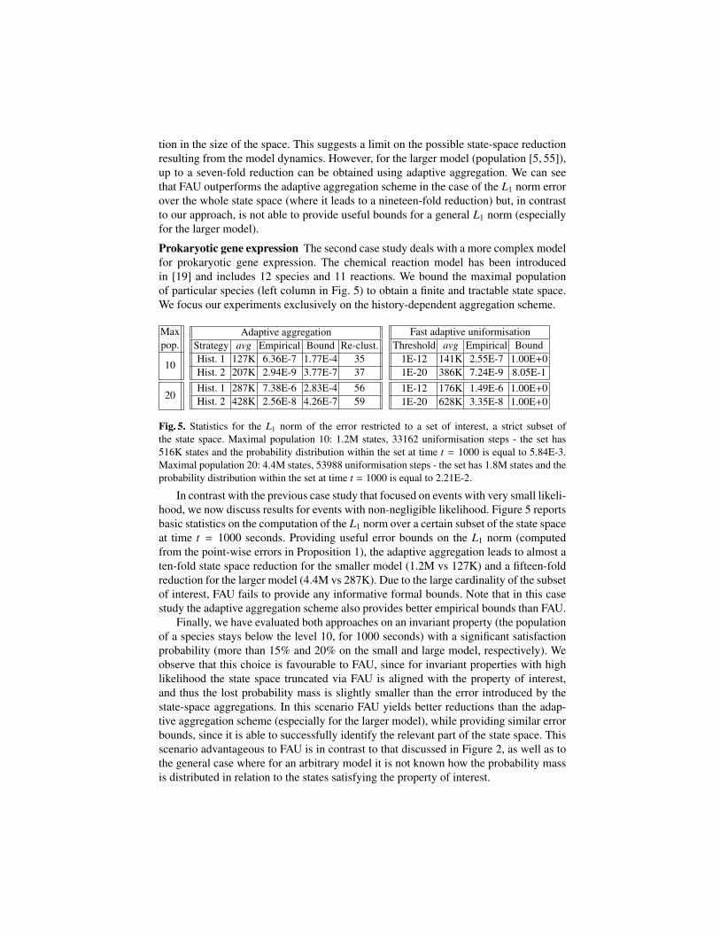
Prokaryotic gene expression The second case study deals with a more complex modelfor prokaryotic gene expression. The chemical reaction model has been introducedin [19] and includes 12 species and 11 reactions. We bound the maximal populationof particular species (left column in Fig. 5) to obtain a finite and tractable state space.We focus our experiments exclusively on the history-dependent aggregation scheme.

Maxpop.

10

20

Adaptive aggregationStrategy avg Empirical Bound Re-clust.Hist. 1 127K 6.36E-7 1.77E-4 35Hist. 2 207K 2.94E-9 3.77E-7 37Hist. 1 287K 7.38E-6 2.83E-4 56Hist. 2 428K 2.56E-8 4.26E-7 59

Fast adaptive uniformisationThreshold avg Empirical Bound

1E-12 141K 2.55E-7 1.00E+01E-20 386K 7.24E-9 8.05E-11E-12 176K 1.49E-6 1.00E+01E-20 628K 3.35E-8 1.00E+0

Fig. 5. Statistics for the L1 norm of the error restricted to a set of interest, a strict subset ofthe state space. Maximal population 10: 1.2M states, 33162 uniformisation steps - the set has516K states and the probability distribution within the set at time t = 1000 is equal to 5.84E-3.Maximal population 20: 4.4M states, 53988 uniformisation steps - the set has 1.8M states and theprobability distribution within the set at time t = 1000 is equal to 2.21E-2.

In contrast with the previous case study that focused on events with very small likeli-hood, we now discuss results for events with non-negligible likelihood. Figure 5 reportsbasic statistics on the computation of the L1 norm over a certain subset of the state spaceat time t = 1000 seconds. Providing useful error bounds on the L1 norm (computedfrom the point-wise errors in Proposition 1), the adaptive aggregation leads to almost aten-fold state space reduction for the smaller model (1.2M vs 127K) and a fifteen-foldreduction for the larger model (4.4M vs 287K). Due to the large cardinality of the subsetof interest, FAU fails to provide any informative formal bounds. Note that in this casestudy the adaptive aggregation scheme also provides better empirical bounds than FAU.

Finally, we have evaluated both approaches on an invariant property (the populationof a species stays below the level 10, for 1000 seconds) with a significant satisfactionprobability (more than 15% and 20% on the small and large model, respectively). Weobserve that this choice is favourable to FAU, since for invariant properties with highlikelihood the state space truncated via FAU is aligned with the property of interest,and thus the lost probability mass is slightly smaller than the error introduced by thestate-space aggregations. In this scenario FAU yields better reductions than the adap-tive aggregation scheme (especially for the larger model), while providing similar errorbounds, since it is able to successfully identify the relevant part of the state space. Thisscenario advantageous to FAU is in contrast to that discussed in Figure 2, as well as tothe general case where for an arbitrary model it is not known how the probability massis distributed in relation to the states satisfying the property of interest.

6 Conclusions

We have proposed a novel adaptive aggregation algorithm for approximating the prob-ability of an event in a Markov chain with rigorous precision guarantees. Our approachprovides error bounds that are in general orders of magnitude more accurate comparedto those from fast adaptive uniformisation, and significantly decreases the size of mod-els without performance degradation. This has allowed us to efficiently analyse largerand more complex models. Future work will include effective combinations of the adap-tive aggregation with robustness analysis and parameter synthesis. We also plan to ap-ply our approach to the verification and performance analysis of complex safety-criticalcomputer systems, where precision guarantees play a key role.

References

1. A. Abate, J.-P. Katoen, J. Lygeros, and M. Prandini. Approximate model checking of stochas-tic hybrid systems. European Journal of Control, 16:624–641, 2010.

2. A. Abate, M. Kwiatkowska, G. Norman, and D. Parker. Probabilistic model checking oflabelled Markov processes via finite approximate bisimulations. In Horizons of the Mind. ATribute to Prakash Panangaden, volume 8464 of LNCS, pages 40–58. Springer, 2014.

3. A. Angius, A. Horvath, and V. Wolf. Quasi product form approximation for Markov mod-els of reaction networks. In Transactions on Computational Systems Biology (TCSB) XIV,volume 7625 of LNCS, pages 26–52. Springer, 2012.

4. C. Baier and J.-P. Katoen. Principles of model checking. The MIT Press, 2008.5. L. Bortolussi and J. Hillston. Fluid model checking. In Concurrency Theory (CONCUR),

volume 7454 of LNCS, pages 333–347. Springer, 2012.6. P. Buchholz. Exact performance equivalence: An equivalence relation for stochastic au-

tomata. Theor. Comput. Sci., 215(1-2):263–287, 1999.7. M. Ceska, D. Safranek, S. Drazan, and L. Brim. Robustness analysis of stochastic biochem-

ical systems. PloS one, 9(4):e94553, 2014.8. T. Chen and S. Kiefer. On the total variation distance of labelled Markov chains. In Computer

Science Logic (CSL) and Logic in Computer Science (LICS), 2014.9. F. Dannenberg, E. M. Hahn, and M. Kwiatkowska. Computing cumulative rewards using fast

adaptive uniformisation. ACM Transactions on Modeling and Computer Simulation, SpecialIssue on Computational Methods in Systems Biology (CMSB), 2014. To appear.

10. J. Desharnais, F. Laviolette, and M. Tracol. Approximate analysis of probabilistic processes:logic, simulation and games. In Quantitative Evaluation of SysTems (QEST), pages 264–273,2008.

11. A. D’Innocenzo, A. Abate, and J.-P. Katoen. Robust PCTL model checking. In HybridSystems: Computation and Control (HSCC), pages 275–285. ACM, 2012.

12. S. Engblom. Computing the moments of high dimensional solutions of the master equation.Applied Mathematics and Computation, 180(2):498 – 515, 2006.

13. L. Ferm and P. Lotstedt. Adaptive solution of the master equation in low dimensions. AppliedNumerical Mathematics, 59(1):187–204, 2009.

14. B. L. Fox and P. W. Glynn. Computing Poisson Probabilities. Communications of the ACM,31(4):440–445, 1988.

15. D. T. Gillespie. Exact Stochastic Simulation of Coupled Chemical Reactions. Journal ofPhysical Chemistry, 81(25):2340–2381, 1977.

16. J. Hasenauer, V. Wolf, A. Kazeroonian, and F. Theis. Method of conditional moments (mcm)for the chemical master equation. Journal of Mathematical Biology, pages 1–49, 2013.

17. M. Hegland, C. Burden, L. Santoso, S. MacNamara, and H. Booth. A solver for the stochasticmaster equation applied to gene regulatory networks. Journal of computational and appliedmathematics, 205(2):708–724, 2007.

18. T. A. Henzinger, M. Mateescu, and V. Wolf. Sliding Window Abstraction for Infinite MarkovChains. In Computer Aided Verification (CAV), volume 5643 of LNCS, pages 337–352.Springer, 2009.

19. A. M. Kierzek, J. Zaim, and P. Zielenkiewicz. The effect of transcription and translationinitiation frequencies on the stochastic fluctuations in prokaryotic gene expression. Journalof Biological Chemistry, 276(11):8165–8172, 2001.

20. M. Kwiatkowska, G. Norman, and D. Parker. PRISM 4.0: Verification of Probabilistic Real-time Systems. In Computer Aided Verification (CAV), volume 6806 of LNCS, pages 585–591.Springer, 2011.

21. K. G. Larsen and A. Skou. Bisimulation through probabilistic testing. Information andComputation, 94(1):1 – 28, 1991.

22. C. Madsen, C. Myers, N. Roehner, C. Winstead, and Z. Zhang. Utilizing stochastic modelchecking to analyze genetic circuits. In Computational Intelligence in Bioinformatics andComputational Biology (CIBCB), pages 379–386. IEEE Computer Society, 2012.

23. M. Mateescu, V. Wolf, F. Didier, and T. A. Henzinger. Fast Adaptive Uniformization of theChemical Master Equation. IET Systems Biology, 4(6):441–452, 2010.

24. B. Munsky and M. Khammash. The finite state projection algorithm for the solution of thechemical master equation. The Journal of chemical physics, 124:044104, 2006.

25. R. Sidje and W. Stewart. A numerical study of large sparse matrix exponentials arising inMarkov chains. Computational statistics & data analysis, 29(3):345–368, 1999.

26. S. E. Z. Soudjani and A. Abate. Adaptive and sequential gridding procedures for the abstrac-tion and verification of stochastic processes. SIAM Journal on Applied Dynamical Systems,12(2):921–956, 2013.

27. S. E. Z. Soudjani and A. Abate. Precise approximations of the probability distribution of aMarkov process in time: an application to probabilistic invariance. In Tools and Algorithmsfor the Construction and Analysis of Systems (TACAS), pages 547–561. Springer, 2014.

28. R. Steuer, S. Waldherr, V. Sourjik, and M. Kollmann. Robust signal processing in livingcells. PLoS computational biology, 7(11):e1002218, 2011.

29. I. Tkachev and A. Abate. On approximation metrics for linear temporal model-checking ofstochastic systems. In Hybrid Systems: Computation and Control (HSCC), pages 193–202.ACM, 2014.

30. A. P. van Moorsel and W. H. Sanders. Adaptive uniformization. Stochastic Models,10(3):619–647, 1994.

31. J. Zhang, L. T. Watson, and Y. Cao. Adaptive aggregation method for the chemical masterequation. International Journal of Computational Biology and Drug Design, 2(2):134–148,2009.