adaptive beamforming for array signal processing in aeroacoustic · pdf file ·...
TRANSCRIPT

Adaptive beamforming for array signal processingin aeroacoustic measurements
Xun Huanga)
State Key Laboratory of Turbulence and Complex Systems, Department of Aeronautics and Astronautics,Peking University, Beijing, 100871, China
Long Bai and Igor VinogradovDepartment of Mechanics and Aerospace Engineering, Peking University, Beijing, 100871, China
Edward PeersDepartment of Aeronautics and Astronautics, Peking University, Beijing, 100871, China
(Received 15 June 2011; revised 4 January 2012; accepted 9 January 2012)
Phased microphone arrays have become an important tool in the localization of noise sources for
aeroacoustic applications. In most practical aerospace cases the conventional beamforming
algorithm of the delay-and-sum type has been adopted. Conventional beamforming cannot take
advantage of knowledge of the noise field, and thus has poorer resolution in the presence of noise
and interference. Adaptive beamforming has been used for more than three decades to address these
issues and has already achieved various degrees of success in areas of communication and sonar. In
this work an adaptive beamforming algorithm designed specifically for aeroacoustic applications is
discussed and applied to practical experimental data. It shows that the adaptive beamforming
method could save significant amounts of post-processing time for a deconvolution method. For
example, the adaptive beamforming method is able to reduce the DAMAS computation time by at
least 60% for the practical case considered in this work. Therefore, adaptive beamforming can be
considered as a promising signal processing method for aeroacoustic measurements.VC 2012 Acoustical Society of America. [DOI: 10.1121/1.3682041]
PACS number(s): 43.60.Fg, 43.60.Jn, 43.28.Ra [DKW] Pages: 2152–2161
I. INTRODUCTION
Beamforming techniques with microphone arrays1–3 are
increasingly being used in the aerospace industry4,5 to local-
ize the distribution of airframe noise to allow the develop-
ment of efficient noise control strategies.6 Airframe noise is
particularly evident during landing when the engines operate
at a low power setting7 and the high lift devices and landing
gear are deployed. Generally, airframe noise is produced by
a fluid–structure interaction of aerodynamic surfaces and the
surrounding turbulent flow.8 Scaled models of airframe com-
ponents, which include high lift devices, landing gear, wheel
wells, and sharp trailing edges, have recently been tested in
wind tunnels and anechoic chambers to investigate aeroa-
coustic related flow mechanisms and localize noise source
distributions using acoustic imaging techniques.9
Beamforming is a technique that uses a sensor array to
visualize the location of a signal of interest.10 Various appli-
cations can be found in radar, sonar, communications, and
medical imaging. Aeroacoustic measurements are, to some
extent, challenging for beamforming because of the poor sig-
nal-to-noise ratio and multipath effects in a traditional aero-
dynamic testing facility.5 To address these issues, a test
facility has to be modified specifically to reduce background
noise and to mitigate wall reflections.11,12 Particular atten-
tion has also been paid to array design in order to reduce the
detrimental effect of the background noise. More design
details can be found in Refs. 4, 13, and 14. On the other
hand, although numerous beamforming methods have been
proposed in the last three decades, the conventional beam-
forming method10 with the delay-and-sum approach and its
variants3,13,15 are still the dominant technique used for aeroa-
coustic measurements.
From the perspective of signal processing, an acoustic
imaging process can be regarded as a convolution between
the array frequency responses and acoustic sources of interest.
The frequency response of the conventional beamforming
method has a wide main lobe and high side lobe peaks, which
masks the signal of interest through convolution, leading to
the well-known limited resolution problem. To address this
issue, several different deconvolution algorithms16–21 have
recently been proposed to post-process conventional beam-
forming results in order to restore the signals of interest.
Nowadays the conventional beamformer with the delay-
and-sum approach is rarely used in sonar, radar, and commu-
nication applications, for which the method was initially
developed. An alternative method, adaptive beamforming, or
the so-called Capon beamforming, has a much better resolu-
tion and interference rejection capability22 and has been
adopted as a de facto method in array signal processing. It is
natural to expect that an adaptive beamformer could be help-
ful to pinpoint aeroacoustic noise sources more accurately
and better minimize the convolution effects,5 which, in turn,
could produce array outputs of higher quality saving the
computational efforts of the aforementioned deconvolution
a)Author to whom correspondence should be addressed. Electronic mail:
2152 J. Acoust. Soc. Am. 131 (3), March 2012 0001-4966/2012/131(3)/2152/10/$30.00 VC 2012 Acoustical Society of America
Au
tho
r's
com
plim
enta
ry c
op
y

methods. However, adaptive beamforming is quite sensitive
to any perturbations and its performance can quickly deterio-
rate below an acceptable level, preventing the direct applica-
tion of present adaptive beamforming methods for
aeroacoustic measurements.
It is generally assumed that errors in array measure-
ments are mainly from steering vectors,23 which are deter-
mined by the relative distances between a signal of interest
and the array microphones. More often than not, a steering
vector deviates from the expected one. Installation of a
microphone array on a vibrating testing facility wall is par-
tially responsible for this problem. Any mismatch in steer-
ing vector leads to significant computational error due to
the sensitive nature of adaptive beamforming. The steering
vector can therefore be regarded within a predefined uncer-
tainty ellipsoid and a robust beamformer24 can be conse-
quently designed to maintain an acceptable accuracy
within the complete uncertainty ellipsoid25 (see references
therein for more details of the approach). Diagonal loading
is the other popular approach to improve the robustness of
an adaptive beamformer. This method has been adopted in
the current work for its simplicity of implementation. The
same approach has already been used in previous aeroa-
coustic measurements.5,26 It can be seen that the perform-
ance of diagonal loading depends on a suitable choice of
loading parameter. An iterative procedure has been
adopted in this work to straightforwardly find an appropri-
ate value of the loading parameter in practical aeroacoustic
tests.
In previous work,5,26 adaptive beamforming for aeroa-
coustics has only been applied for numerical benchmark
cases or idealized cases with speakers as experimental noise
sources. To the best of our knowledge, there is no literature
dealing with development and/or application of adaptive
beamforming for practical aeroacoustic setups. Because the
only way to validate an algorithm is to apply it for practical
applications, the main contribution of this work fills the gap,
using an adaptive beamforming for one of the landing gear
components. First, the adaptive beamforming algorithm
developed specifically for aeroacoustics is proposed in
Sec. II. The experimental setup of the aeroacoustic test is
summarized in Sec. III and the related acoustic imaging
results are reviewed in Sec. IV. Advantages and shortcom-
ings of adaptive beamforming for aeroacoustics are dis-
cussed in Sec. V.
II. FORMULATIONS
A. Sound field model
The notations that generally appear in the literature5,23
are adopted in the following. Given a microphone array with
M microphones, the output x(t) denotes time domain meas-
urements of microphones, x 2 <M�1 and t denotes time. For
a single signal of interest s tð Þ 2 <1 in a free sound propaga-
tion space, using Green’s function for the wave equation in a
free space, we can have
x tð Þ ¼ 1
4prs t� sð Þ; s ¼ r
C; (1)
where C is the speed of sound, r 2 <M�1 are the distances
between the signal of interest s and microphones, and s is
the related sound propagation time delay between s and the
microphones. For most aeroacoustic applications, beam-
forming is generally conducted in the frequency domain.18
The frequency domain version of Eq. (1) is
XðjxÞ ¼ 1
4prSðjxÞe�jxs ¼ a0 r; jxð ÞSðjxÞ; (2)
where j ¼ffiffiffiffiffiffiffi�1p
, a0 is the steering vector, x is angular fre-
quency, (jx) and (r, jx) can be omitted for brevity, X and Sare counterparts in the frequency domain, and we can simply
write Eq. (2) as X¼ a0S.The situation becomes more complex for a practical
case, for which the array output vector can be represented as
X ¼ a0Sþ Iþ N; (3)
where I is the interference from coherent signals and/or
reflections and N denotes the collective error from facility
background noise and sensor noise. It is worthwhile to note
that the signal of interest (S), interference (I), and noise (N)
are of zero-mean signal waveforms, and S and N are gener-
ally assumed statistically independent for simplicity.
Let RX, RIN, and RS denote the M�M theoretical covar-
iance matrix (also known as the cross spectrum matrix or
cross-spectral density matrix) of the array output vector and
interference-plus-noise covariance and signal of interest co-
variance matrices, respectively; and then we have
Rx ¼ E XX�f g; (4)
RIN ¼ E Iþ Nð Þ Iþ Nð Þ�f g; (5)
RS ¼ E a2a0a�0� �
¼ RX � RIN ; if E X Iþ Nð Þ�¼ 0f g;(6)
where (�)* stands for conjugate transpose, E{�} denotes the
statistical expectation, and r2 ¼ Ef Sj j2g is the variance of S.In practical aeroacoustic measurements, N denotes back-
ground noise that can be measured separately without the
presence of any test model, which is a practice generally
adopted in aeroacoustic experiments.4,9,17,18 The measure-
ments of X can be conducted thereafter with the placement
of a test model within the test section. The statistics of the
signal of interest r2 can be subsequently estimated and a
suitable beamforming method with a narrow main lobe and
small side lobes can reduce interference from unknown I.
The assumption of E {X(IþN)*¼ 0} suggests that no corre-
lation between the signal of interest and the interference plus
the facility background noise. The assumption is normally
valid in most aeroacoustic experiments and therefore has
been widely adopted.17,18 For the correlated case, a so-called
observer-based beamforming method has been proposed in
the literature13,27,28 to address the issue.
In practical applications, the covariance matrix R is
approximated by sample covariance matrices, which are con-
structed based on array samples X and N. We can have
J. Acoust. Soc. Am., Vol. 131, No. 3, March 2012 Huang et al.: Adaptive beamforming for aeroacoustics 2153
Au
tho
r's
com
plim
enta
ry c
op
y
RX �1
K
XK
k¼1
XX�; (7)
where the caret denotes approximations and K is the number
of sampling blocks which is preferably a large number (e.g.,
100 was empirically chosen in experiments), compared to
the period of signal of interest, for statistical confidence. In
addition, RIN has to be approximated in the following form
as the interference I is largely unknown:
RIN �1
K
XK
k¼1
NN�: (8)
And finally the approximation for RS is
RS � RX � RIN: (9)
B. Conventional beamforming
A narrowband beamformer output for each frequency
bin of interest can be written as
Y ¼W�X; (10)
where Y is the beamformer output and W 2 CM�1 is the
beamformer weight vector. For the conventional beam-
former of delay-and-sum type, the beamformer weight vec-
tor is obtained by minimizing the approximation error10
minw
W�W subject to W�a0 ¼ 1: (11)
It is easy to see that the solution is Wopt ¼ a0a�0� ��1
a0 yield-
ing the following estimation of r2:
r2 ¼W�optRSWopt ¼ a�0 a0a�0
� ��1RS a0a�0� ��1
a0; (12)
where RS can be approximated with Eq. (9) in experiments
and a0 can be obtained with array geometry and experimen-
tal setup details.
C. Adaptive beamforming
The fundamental idea behind Capon beamforming is to
obtain Wopt through maximizing the signal-to-interference-
plus ratio (SINR),
SINR ¼ W�RSW
W�RINW; (13)
and maintaining distortionless response toward the direction
of the signal of interest.23,29 In other words, the expected
effect of the noise and interferences should be minimized,
thus leading to the following linearly constrained quadratic
problem:30
minW
W�RINW subject to W�a0 ¼ 1; (14)
The solution can be obtained with a Lagrange multiplier,10
i.e., Wopt ¼ aR�1IN a0, where a is a constant that equals
a�0R�1IN a0
� ��1. In practical aeroacoustic applications the co-
variance matrix RIN is unavailable and has to be approxi-
mated by the sampling covariance matrix RX. We can have
r2 ¼ W�optRSWopt; (15)
where Wopt ¼ R�1
x a0=a�0R�1
x a0 and RS can be obtained using
Eq. (9). It is worthwhile to mention that Eq. (15) is different
from the classical form of adaptive beamforming,
r2 ¼ W�optRSWopt; (16)
where Wopt is the same as that in Eq. (15), whose solutions
contain both background noise and the desired signal.
Hence, Eq. (16) is not adopted in this work. In addition, the
covariance matrix of the desired signal RX and the noise RIN
can be approximated using Eqs. (8) and (9), respectively.
One could also propose another alternative adaptive beam-
forming algorithm as shown in
r2 ¼ W�optRSWopt; (17)
where Wopt ¼ R�1
IN a0=a�0R�1
IN a0. In this work we found that
this algorithm fails to generate satisfactory results for practi-
cal data. The potential reason could be mismatches in back-
ground noise covariance matrices. That is, RIN in Eq. (17) is
obtained without the presence of any test model. The instal-
lation of a test model, however, could alter the background
noise covariance matrix. As a result, Eq. (15) is adopted in
this paper for adaptive beamforming implementation.
It is worthwhile to emphasize that the method [Eq. (14)]
was originally proposed for rank-one signal (point source)
cases. However, the number of discrete noise sources distrib-
uted in a practical aeroacoustic case could be larger than the
number of array microphones. As a result, RX could have a
full rank. The direct application of Eq. (15) [the solution of
Eq. (14)] for acoustic imaging could lead to questionable
results. Hence, specific modifications of RX have to be con-
ducted, the details of which can be found in Sec. IV.
D. Robust adaptive beamforming
The main objective of this paper is to investigate the
performance of adaptive beamforming in practical aeroa-
coustic applications. In previous work we have already dem-
onstrated that conventional beamforming with a delay-and-
sum approach is independent of sample data and has been
successfully applied for various aeroacoustic cases.13,31,32 In
contrast, the adaptive beamforming method is well known
for its great sensitivity to any mismatches, perturbations, and
data errors. A systematic solution has been proposed to
improve the robustness of adaptive beamforming with
respect to any mismatches in steering vectors.23,25 In this
work the array is placed outside of the free stream and
should have little mismatch in steering vector (detailed setup
is given in the next section). It is therefore assumed that the
main computational error of an adaptive beamformer should
2154 J. Acoust. Soc. Am., Vol. 131, No. 3, March 2012 Huang et al.: Adaptive beamforming for aeroacoustics
Au
tho
r's
com
plim
enta
ry c
op
y
come from the ill-conditioning of sample matrices. Regulari-
zation methods can be used to mitigate the ill-conditioning
by adding a suitable constant to diagonal elements of sample
matrices. This is the so-called diagonal loading technique,
which is one of the most popular approaches for robust
adaptive beamforming. The regularized problem can be
described by
minW
W�RINWþ �W�W subject to W�a0 ¼ 1; (18)
where the diagonal loading factor � imposes a penalty to
avoid an inappropriately large array vector W. The diagonal
loaded version of Eq. (15) is
r2 ¼ W�optRSWopt; (19)
where Wopt ¼ RX þ �IM
� ��1a0=a�0 RX þ �IM
� ��1a0 and IM is
the M�M identity matrix. It is easy to see that the diagonal
loading ensures the invertibility of the loaded matrix
RX þ �IM regardless of weather RX is ill-conditioned.
The choice of the diagonal loading factor � is somewhat
ad hoc. Empirical criteria for � with respect to the so-called
white noise gain parameter has been given previously.16 The
latter parameter depends on physical insights. For simplicity,
an iterative procedure is used in this work to tune �, which is
set to k max [eig(RX)], eig (�) denotes the eigenvalues of a
matrix. The diagonal loading parameter k can be iteratively
chosen between 0.01 and 0.5. A smaller k normally produces
an image with better resolution, but the computation can fail
due to numerical instability. The computational failure is
determined by comparing the maximal sound pressure val-
ues. Once the difference between the classical beamforming
result and the adaptive beamforming result exceeds a thresh-
old (empirically set to 3 dB), the adaptive beamforming
computation fails. The value of k is thus improper and has to
be enlarged. On the other hand, a larger k generates a result
similar to that of a conventional beamformer. This finding is
understandable as a big k leads to a heavy penalty � in the
optimization in Eq. (19) that therefore approaches Eq. (11).
For the following practical case we found that the value
of k can be quickly determined within a couple of iterations.
The diagonal loading approach is hence used in the rest of
this paper for its simplicity of implementation. In summary
the beamforming algorithm for a narrowband frequency
range is conducted as follows:
Step 1: Compute sample covariance matrices RX and RS,
and compute eigenvalues of RX.
Step 2: Given an observed plane, which has N gridpoints,
construct steering vector a0 for each gridpoint.
Step 3: Calculate the diagonal loading factor � with an initial
guess of k¼ 0.01. �¼ k max [eig(RX)].
Step 4: Repeat the adaptive beamforming equation
[Eq. (19)] at each of N gridpoints to produce the acoustic
image.
Step 5: Qualitative check. The whole computation is com-
pleted if the quality is satisfactory and no numerical insta-
bility appears. Otherwise double the value of k and repeat
steps 3–5.
E. Deconvolution approach
Various deconvolution algorithms(16–21) have been
proposed to post-process beamforming results. The deconvo-
lution approach for the mapping of acoustic sources
(DAMAS)17 was adopted in this work. For convenience of
readers, the fundamental idea behind DAMAS is briefly
introduced in the following.
The DAMAS approach resolves an inverse problem,
Z¼AS, where Z 2 CN�1 are the N estimations of each grid-
point, using Eq. (12) or Eq. (19), respectively; S 2 CN�1 rep-
resents sound sources at each gridpoint and A 2 CN�N is
formed by the steering vectors, relating Z to S. The acoustic
images shown in this work have 121� 121 gridpoints and
N¼ 14 641. It is thus extremely difficult to calculate the
inverse of A. An iterative scheme has been proposed17 to
estimate S from Z, instead of the direct calculation of the
inverse of A. As a result, the resolution of acoustic images
could be extensively improved. For brevity, details of the
algorithms are omitted. The interested reader should refer to
the literature.17
III. EXPERIMENTAL APPARATUS
To test the performance, the above adaptive signal proc-
essing algorithm is applied for a practical aeroacoustic case.
The experiments have been conducted in an anechoic chamber
facility (9.15 m� 9.15 m� 7.32 m) at ISVR, University of
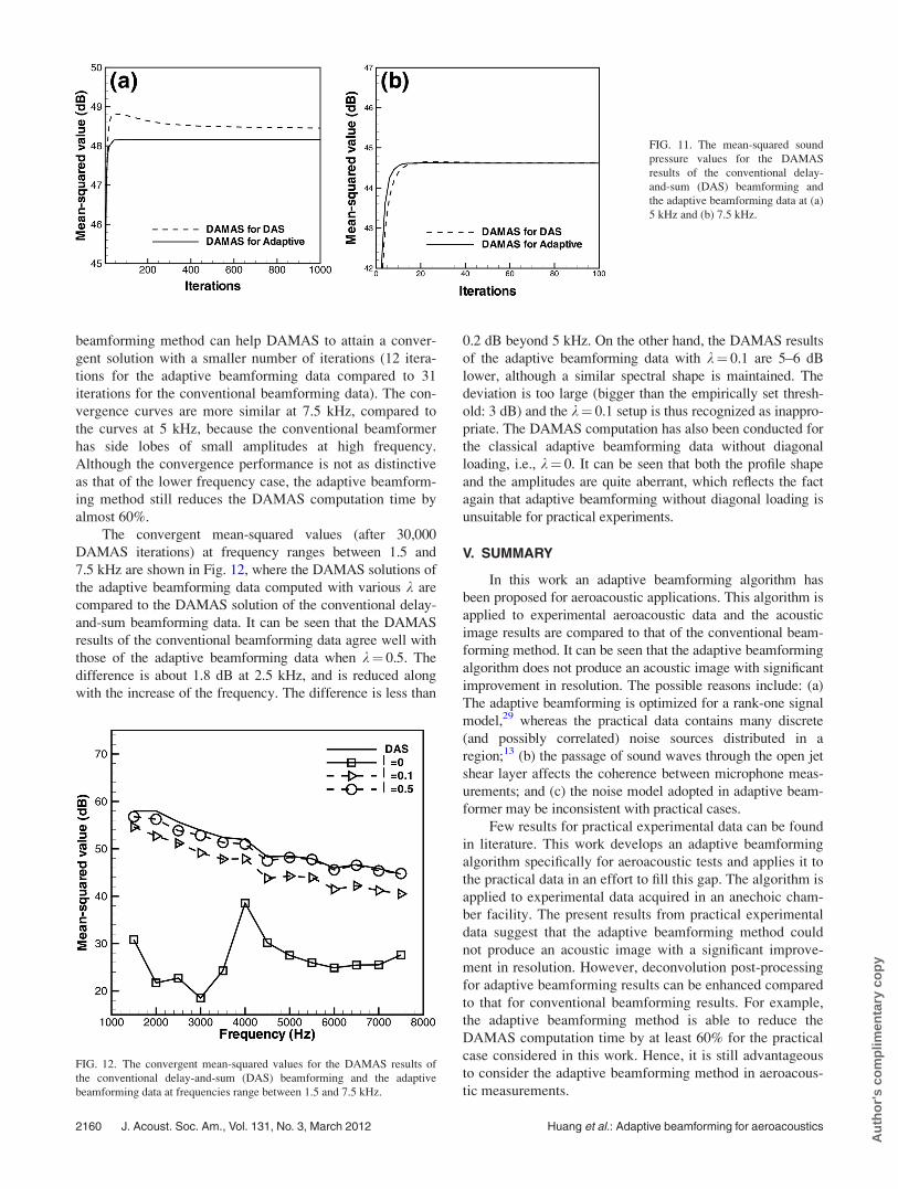
Southampton. Figure 1 shows the complete setup. A nozzle
(500 mm � 350 mm) connecting to a plenum chamber can
produce a jet flow of U1¼ 30 m/s. An array with 56 electret
microphones (Panasonic WM-60A) is placed on the ground.
The sensitivity of each microphone is �45 6 5 dBV/Pa. The
frequency response (amplitude and phase) of each microphone
is calibrated to a B&K 4189 microphone in order to reduce in-
herent amplitude and phase differences between array micro-
phones. An airframe model representing a part of a landing
gear was placed right above the microphone array. The coordi-
nates shown in Fig. 1 are used throughout the rest of the paper.
The coordinate origin is at the center of the link structure of
the triangle shape. The center of the array is aligned with the
origin, and the distance from the origin is 0.7 m.
Figure 2 shows a photograph of the experimental setup
in the test section. Two endplates are used to hold the bluff
FIG. 1. (Color online) The illustration of the setup of experiment units (not
to scale).
J. Acoust. Soc. Am., Vol. 131, No. 3, March 2012 Huang et al.: Adaptive beamforming for aeroacoustics 2155
Au
tho
r's
com
plim
enta
ry c
op
y

body model and maintain two-dimensional free stream flow
in the open test section. A pitot tube is placed in front of the
model to measure the free stream speed. The array is under-
neath the model. The shear layer correction based on Snell’s
law9 is used in the beamforming signal processing as the
array is placed outside of the testing flow. Measurements
have also been conducted for a separate scenario without the
presence of the model to approximate the facility back-
ground noise.
The size of the complete array is 1 m� 1 m. The effec-
tive diameter is 0.64 m, within which microphones are
deployed. The layout of microphones was designed for the
particular purpose of reducing spatial aliasing.9 The accu-
racy of the microphone locations is within 1 mm. In addition,
the array was placed outside of testing flow and firmly fas-
tened to the ground to prevent any flow induced vibration,
reducing the chance of any potential mismatch in the steer-
ing vectors of the array.
An NI PXI-1033 chassis with four 24 bit PXI-4496
cards has been used to simultaneously sample 56 channels of
microphones at 44 000 samples/s. Each data acquisition is
operated through a band pass filter to remove the direct cur-
rent part and to avoid high frequency aliasing. The data
stream is cut into consecutive blocks, and each block con-
tains 4096 samples for the discrete Fourier transform (DFT).
The DFT amplitudes of each microphone are calibrated to a
sound source of 96 dB at 1 kHz, and the decibel values are
referenced to 2� 10�5Pa.
IV. RESULTS AND DISCUSSION
A literature review shows that most previous work is
focused on numerical examples. However, an application of
an algorithm to experimental data is required to determine
its applicability. In this work a practical aeroacoustic case
involving a bluff body model is considered.
Figure 3 shows nondimensionalized acoustic image
results at f¼ 5 kHz. The two horizontal lines in Fig. 3 repre-
sent the two endplates that help to maintain a better quality
of test flow. The rest of the sketch illustrates the bluff body
model. Two triangle-shaped bodies represent the compo-
nents installed on the cylinder model, which are intentionally
removed in Figs. 3(b)–3(d) to clearly show acoustic images.
The whole bluff body is an idealized model of the main ele-
ments of an aircraft landing gear. The free stream direction
FIG. 2. (Color online) Overall system working in an anechoic chamber.
FIG. 3. (Color online) Acoustic
image for the practical aeroacoustic
case with a bluff body model, (a) the
adaptive beamforming method [with
Eq. (19) at k¼ 0], (b) the adaptive
beamforming method [with Eq. (19)
at k¼ 0.1], (c) the adaptive beam-
forming method [with Eq. (19) at
k¼ 0.5], and (d) the conventional
beamforming method [with Eq.
(12)], respectively. f¼ 5 kHz and
U1¼ 30 m/s.
2156 J. Acoust. Soc. Am., Vol. 131, No. 3, March 2012 Huang et al.: Adaptive beamforming for aeroacoustics
Au
tho
r's
com
plim
enta
ry c
op
y

of the open jet is from the left to the right. All experiments
have been conducted at U1¼ 30 6 0.5 m/s. The correspond-
ing Reynolds number with respect to the cylinder diameter is
in the order of 105. The dominant flow-induced noise sources
are located at the links [A–C in Fig. 3(b)]. More details
related to the test model and related flow-induced noise
mechanisms can be found in Ref. 31, whereas the attention
of this paper is focused on the array signal processing
method.
Figure 3(a) is the acoustic image obtained with Eq. (19)
but without diagonal loading (k and � equal 0). This figure
contains chaotic acoustic imaging patterns with much lower
sound pressure (see the upcoming Fig. 12), which suggests
that the adaptive beamforming method without diagonal load-
ing fails to identify dominant noise sources for practical aeroa-
coustic data. Any discrepancy in experimental measurements,
such as multipath propagation, background noise or interfer-
ence from coherent signals, and the mismatching of steering
vectors, can lead to failure of adaptive beamformers.
Diagonal loading is used to address the issue, although
the determination of a suitable diagonal loading parameter
remains an open problem. For the case considered in this
work, k¼ 0.1 and k¼ 0.5 have been tested and results are
shown in Figs. 3(b) and 3(c), respectively. Both figures show
that the background noise from the open jet has been
rejected. Compared to the conventional beamforming results
shown in Fig. 3(d), the positions and amplitudes of the domi-
nant noise sources at the middle locations of the model agree
well. Dynamic ranges of both adaptive beamforming and
conventional beamforming results are quite similar, whereas
the resolution has been improved. In addition, the resolution
of Fig. 3(b) with k¼ 0.1 is somewhat better than that of Fig.
3(c) with k¼ 0.5. In contrast the resolution of the conven-
tional beamforming results is relatively low and some cha-
otic patterns can be found in Fig. 3(d), which are caused by
the relatively high side lobes of the conventional beamform-
ing method. It is worthwhile to point out that weights can be
optimized (such as applying a window technique) to lower
the side lobes. However, the width of the main lobe will be
increased and the resolution will thus be sacrificed.
The adaptive beamforming method fails to improve re-
solution extensively for this practical case. This outcome
answers the question frequently raised by signal processing
experts: Why is adaptive beamforming so rarely used in
aeroacoustic measurements? However, for its distinctive
side lobe suppression capability, the adaptive beamforming
method can generate images with less spurious patterns,
which could save huge amounts of post-processing time for
a deconvolution method. DAMAS17 has been conducted for
the case to demonstrate the idea.
Figure 4 shows DAMAS results after 1000 iterations,
which are initially post-processed on the conventional beam-
forming result [Fig. 3(d)] and the adaptive beamforming result
[Fig. 3(b)], respectively. The noise sources in Fig. 4(a) fail to
form a distinctive pattern and therefore show less physical
insight. In contrast, the individual noise sources in Fig. 4(b)
are clearly distributed along the triangle parts (excluded for
clarity). This finding supports the above-mentioned statement
regarding the adaptive beamforming method.
All beamforming methods introduced in this work were
developed in MATLAB and computed on a desktop with an
Intel i7 CPU (920 @ 2.67 GHz) and 8 GB memory. The
code spent 110 s for the DAMAS method to finish 1000 iter-
ations. It took an additional 30 000 iterations for Fig. 4(a) to
achieve a pattern similar to that of Fig. 4(b). Hence, the
adaptive beamforming method can help DAMAS quickly
approach a reasonable source distribution. As a result, it is
advantageous to consider adaptive beamforming in aeroa-
coustics. It is also worthwhile to point out that the conven-
tional beamforming required 0.98 s to perform the
calculation, whereas the adaptive beamforming required 1 s
for the same case. These data are given here just for the read-
ers’ information as no particular optimization has been con-
ducted for our code.
Acoustic images at various frequencies are shown in
Figs. 5–8 to further illustrate the performance of beamform-
ing methods. Figures 5(a) and 5(b) present acoustic image
results at f¼ 2.5 kHz using the conventional beamforming
method and the adaptive beamforming method, respectively.
The adaptive beamforming method is unable to realize a re-
solution advantage. However, again, DAMAS post-
processing results can reveal the superior quality of the
adaptive beamforming. Figure 6 shows the related results of
1000 DAMAS iterations. It can be seen that the DAMAS
results for the conventional beamforming indicate a source
distribution along the trailing triangle parts, whereas the
DAMAS results for the adaptive beamforming identify the
main noise sources at the links [A–C in Fig. 3(b)].
Figures 7(a) and 7(b) are acoustic images at f¼ 7.5 kHz
by conventional beamforming and adaptive beamforming,
FIG. 4. (Color online) The DAMAS
post-processing outcomes (1000
iterations) of the results of (a) con-
ventional beamforming and (b)
adaptive beamforming (k¼ 0.5) in
Fig. 3, where f¼ 5 kHz.
J. Acoust. Soc. Am., Vol. 131, No. 3, March 2012 Huang et al.: Adaptive beamforming for aeroacoustics 2157
Au
tho
r's
com
plim
enta
ry c
op
y

FIG. 5. (Color online) Acoustic
image results of the practical aeroa-
coustic case, (a) the conventional
beamforming method [with Eq.
(12)] and (b) the adaptive beam-
forming method [with Eq. (19)] with
diagonal loading at k¼ 0.5, where
f¼ 2.5 kHz.
FIG. 6. (Color online) The DAMAS
post-processing outcomes (1000 iter-
ations) of the results of (a) conven-
tional beamforming and (b) adaptive
beamforming (k¼ 0.5) in Fig. 5,
where f¼ 2.5 kHz.
FIG. 7. (Color online) Acoustic
image results of the practical aeroa-
coustic case, (a) the conventional
beamforming method [with Eq.
(12)] and (b) the adaptive beam-
forming method [with Eq. (19)] with
diagonal loading at k¼ 0.5, where
f¼ 7.5 kHz.
FIG. 8. (Color online) The DAMAS
post-processing outcomes (1000
iterations) of the results of (a) con-
ventional beamforming and (b)
adaptive beamforming (k¼ 0.5) in
Fig. 7, where f¼ 7.5 kHz.
2158 J. Acoust. Soc. Am., Vol. 131, No. 3, March 2012 Huang et al.: Adaptive beamforming for aeroacoustics
Au
tho
r's
com
plim
enta
ry c
op
y

respectively. It can be seen that the acoustic image results at
this higher frequency include some chaotic patterns, which
are mainly caused by array sidelobes that are typically higher
at higher frequencies for a given array design. The potential
loss of sensitivity during the passage of the acoustic waves
through the open jet shear layer could be the other cause. A
high frequency sound suffers loss more than the low fre-
quency sound, as the former’s wavelength is more compara-
ble to the characteristic width of the shear layer. Figure 8
shows the post-processing results of 1000 DAMAS itera-
tions. It can be seen that adaptive beamforming helps to pro-
duce a DAMAS result with more distinctive noise
distributions. It is also worthwhile to mention that a similar
improvement is expected for other post-processing methods,
such as CLEAN.18 All results in Figs. 9–12 are shown in a nor-
malized form. A calibration can be conducted to achieve
absolute sound levels, which are shown in Fig. 9.
To quantitatively show the performance of different
beamforming methods, sound pressure squared-mean values
of the grid points within an integration region are summed
up. Similar operations can be found in the literature.17 The
integration region is represented by a dashed rectangle in
Fig. 10, which covers the dominant noise sources and is
deliberately kept away from the two endplates, where the
turbulent boundary flow affects acoustic measurements.
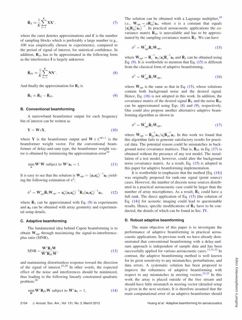
The total amount of the mean-squared values within the
integration region is shown in Fig. 11. For the 5 kHz beam-
forming results [Fig. 11(a)], it can be seen that the total noise
converges rapidly for the adaptive beamforming data. The
total noise is within 1 dB after 10 DAMAS iterations and
within 0.01 dB after 100 iterations. In contrast, the total
noise converges much slower in the case of the conventional
beamforming data. The total noise converges within 1 dB af-
ter 15 iterations. However, after 300 iterations, the conver-
gence speed slows down to less than 0.01 dB per 100
iterations. Convergence is still not achieved after 10 000 iter-
ations (which is not shown here for brevity). Similar findings
have been reported for low frequency cases in literature.17
These two results suggest that the adaptive beamforming
method used here can extensively reduce the required post-
processing effort for DAMAS.
It has also been found that DAMAS results converge
more quickly for high frequency cases.17 The same experi-
ments have been conducted for the 7.5 kHz case and the
results are shown in Fig. 11(b). Once again, the adaptive
FIG. 9. (Color online) The DAMAS
post-processing outcomes (10 000
iterations, k¼ 0.5), where (a,b) f¼5 kHz and (c,d) f¼ 7.5 kHz; (a) and
(c) are DAMAS results for the con-
ventional beamforming solutions; (b)
and (d) are DAMAS results for the
adaptive beamforming solutions.
FIG. 10. (Color online) The mean-squared sound pressure values are
summed within the dashed rectangular integration region.
J. Acoust. Soc. Am., Vol. 131, No. 3, March 2012 Huang et al.: Adaptive beamforming for aeroacoustics 2159
Au
tho
r's
com
plim
enta
ry c
op
y
beamforming method can help DAMAS to attain a conver-
gent solution with a smaller number of iterations (12 itera-
tions for the adaptive beamforming data compared to 31
iterations for the conventional beamforming data). The con-
vergence curves are more similar at 7.5 kHz, compared to
the curves at 5 kHz, because the conventional beamformer
has side lobes of small amplitudes at high frequency.
Although the convergence performance is not as distinctive
as that of the lower frequency case, the adaptive beamform-
ing method still reduces the DAMAS computation time by
almost 60%.
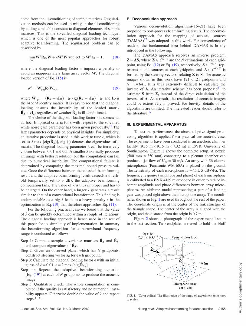
The convergent mean-squared values (after 30,000
DAMAS iterations) at frequency ranges between 1.5 and
7.5 kHz are shown in Fig. 12, where the DAMAS solutions of
the adaptive beamforming data computed with various k are
compared to the DAMAS solution of the conventional delay-
and-sum beamforming data. It can be seen that the DAMAS
results of the conventional beamforming data agree well with
those of the adaptive beamforming data when k¼ 0.5. The
difference is about 1.8 dB at 2.5 kHz, and is reduced along
with the increase of the frequency. The difference is less than
0.2 dB beyond 5 kHz. On the other hand, the DAMAS results
of the adaptive beamforming data with k¼ 0.1 are 5–6 dB
lower, although a similar spectral shape is maintained. The
deviation is too large (bigger than the empirically set thresh-
old: 3 dB) and the k¼ 0.1 setup is thus recognized as inappro-
priate. The DAMAS computation has also been conducted for
the classical adaptive beamforming data without diagonal
loading, i.e., k¼ 0. It can be seen that both the profile shape
and the amplitudes are quite aberrant, which reflects the fact
again that adaptive beamforming without diagonal loading is
unsuitable for practical experiments.
V. SUMMARY
In this work an adaptive beamforming algorithm has
been proposed for aeroacoustic applications. This algorithm is
applied to experimental aeroacoustic data and the acoustic
image results are compared to that of the conventional beam-
forming method. It can be seen that the adaptive beamforming
algorithm does not produce an acoustic image with significant
improvement in resolution. The possible reasons include: (a)
The adaptive beamforming is optimized for a rank-one signal
model,29 whereas the practical data contains many discrete
(and possibly correlated) noise sources distributed in a
region;13 (b) the passage of sound waves through the open jet
shear layer affects the coherence between microphone meas-
urements; and (c) the noise model adopted in adaptive beam-
former may be inconsistent with practical cases.
Few results for practical experimental data can be found
in literature. This work develops an adaptive beamforming
algorithm specifically for aeroacoustic tests and applies it to
the practical data in an effort to fill this gap. The algorithm is
applied to experimental data acquired in an anechoic cham-
ber facility. The present results from practical experimental
data suggest that the adaptive beamforming method could
not produce an acoustic image with a significant improve-
ment in resolution. However, deconvolution post-processing
for adaptive beamforming results can be enhanced compared
to that for conventional beamforming results. For example,
the adaptive beamforming method is able to reduce the
DAMAS computation time by at least 60% for the practical
case considered in this work. Hence, it is still advantageous
to consider the adaptive beamforming method in aeroacous-
tic measurements.
FIG. 11. The mean-squared sound
pressure values for the DAMAS
results of the conventional delay-
and-sum (DAS) beamforming and
the adaptive beamforming data at (a)
5 kHz and (b) 7.5 kHz.
FIG. 12. The convergent mean-squared values for the DAMAS results of
the conventional delay-and-sum (DAS) beamforming and the adaptive
beamforming data at frequencies range between 1.5 and 7.5 kHz.
2160 J. Acoust. Soc. Am., Vol. 131, No. 3, March 2012 Huang et al.: Adaptive beamforming for aeroacoustics
Au
tho
r's
com
plim
enta
ry c
op
y
ACKNOWLEDGMENTS
The majority of this research was supported by the
National Science Foundation grant of China (Grant Nos.
11172007, 11050110109, and 11110072). The experiments
were conducted at ISVR, University of Southampton. We
acknowledge Professor Xin Zhang for his support in the
experiments.
1D. R. Morgan and T. M. Smith, “Coherence effects on the detection
performance of quadratic array processors, with applications to large-
array matched-field beamforming,” J. Acoust. Soc. Am. 87, 737–747
(1990).2D. E. Dudgeon, “Fundamentals of digital array processing,” Proc. IEEE
65, 898–904 (1977).3Y. Liu, A. R. Quayle, A. P. Dowling, and P. Sijtsma, “Beamforming cor-
rection for dipole measurement using two-dimensional microphone
arrays,” J. Acoust. Soc. Am. 124, 182–191 (2008).4H. C. Shin, W. R. Graham, P. Sijtsma, C. Andreou, and A. C. Faszer,
“Implementation of a Phased Microphone array in a closed-section wind
tunnel,” AIAA J. 45, 2897–2909 (2007).5R. A. Gramann and J. W. Mocio, “Aeroacoustic measurements in wind
tunnels using adaptive beamforming methods,” J. Acoust. Soc. Am. 97,
3694–3701 (1995).6X. Huang, S. Chan, X. Zhang, and S. Gabriel, “Variable structure model
for flow-induced tonal noise control with plasma actuators,” AIAA J. 46,
241–250 (2008).7X. X. Chen, X. Huang, and X. Zhang, “Sound radiation from a bypass
duct with bifurcations,” AIAA J. 47, 429–436 (2009).8M. J. Lighthill, “On sound generated aerodynamically. I. General theory,”
Proc. R. Soc. London Ser. A 221, 564–587 (1952).9P. T. Soderman and C. S. Allen, “Microphone measurements in and out of
stream,” in Aeroacoustic Measurements, edited by T. J. E. Mueller
(Springer, New York, 2002), Chap. 1, pp. 26–41.10B. D. Van Veen and K. M. Buckley, “Beamforming: A versatile approach
to spatial filtering,” IEEE ASSP Mag. 5, 4–24 (1988).11M. C. Remillieux, E. D. Crede, H. E. Camargo, R. A. Burdisso, W. J.
Devenport, M. Rasnick, P. V. Seeters, and A. Chou, “Calibration and dem-
onstration of the new Virginia Tech anechoic wind tunnel,” 14th AIAA/
CEAS Aeroacoustics Conference and 29th AIAA Aeroacoustics Confer-
ence, Vancouver, May 2008, AIAA Paper No. 2008-2911.12E. Sarradj, C. Fritzsche, T. Geyer, and J. Giesler, “Acoustic and aerody-
namic design and characterization of a small-scale aeroacoustic wind
tunnel,” Appl. Acoust. 70, 1073–1080 (2009).13X. Huang, “Real-time algorithm for acoustic imaging with a microphone
array,” J. Acoust. Soc. Am. 125, EL190–EL195 (2009).
14X. Huang, I. Vinogradov, L. Bai, and J. C Ji, “Observer for phased micro-
phone array signal processing with nonlinear output,” AIAA J. 48,
2702–2705 (2010).15L. Bai and X. Huang, “Observer-based beamforming algorithm for acous-
tic array signal processing,” J. Acoust. Soc. Am 130, 3803–3811 (2011).16Y. W. Wang, J. Li, P. Stoica, M. Sheplak, and T. Nishida, “Wideband
RELAX and wideband CLEAN for aeroacoustic imaging,” J. Acoust. Soc.
Am. 115, 757–767 (2004).17T. F. Brooks and W. M. Humphrey, “A deconvolution approach for the
mapping of acoustic sources (DAMAS) determined from phased micro-
phone arrays,” J. Sound Vib. 294, 858–879 (2006).18P. Sijtsma, “CLEAN based on spatial source coherence,” Int. J. Aeroa-
coust. 6, 357–374 (2007).19T. Yardibi, J. Li, P. Stoica, and L. N. Cattafesta, “Sparsity constrained
deconvolution approaches for acoustic source mapping,” J. Acoust. Soc.
Am. 123, 2631–2642 (2008).20P. A. Ravetta, R. A. Burdisso, and W. F. Ng, “Noise source localization
and optimization of phased-array results,” AIAA J. 47, 2520–2533 (2009).21T. Yardibi, J. Li, P. Stoica, N. S. Zawodny, and L. N. Cattafesta III, “A co-
variance fitting approach for correlated acoustic source mapping,” J.
Acoust. Soc. Am. 127, 2920–2931 (2010).22O. L. Frost, “An algorithm for linearly constrained adaptive array proc-
essing,” Proc. IEEE 60, 926–935 (1972).23P. Stoica, Z. S. Wang, and J. Li, “Robust Capon beamforming,” IEEE Sig-
nal Proc. Lett. 10, 172–175 (2003).24H. Cox, R. M. Zeskind, and M. M. Owen, “Robust adaptive beamforming,”
IEEE Trans. Acoust. Speech. Sig. Proc. ASSP-35, 1365–1376 (1987).25Z. S. Wang, J. Li, P. Stoica, T. Nishida, and M. Sheplak, “Constant-beam-
width and constant -powerwidth wideband robust Capon beamformers for
acoustic imaging,” J. Acoust. Soc. Am. 116, 1621–1631 (2004).26Y. T. Cho and M. J. Roan, “Adaptive near-field beamforming techniques
for sound source imaging,” J. Acoust. Soc. Am. 125, 944–957 (2009).27L. Bai and X. Huang, “Observer-Based Method in Acoustic Array Signal
Processing,” 16th AIAA/CEAS Aeroacoustics Conference and 31stAIAA Aeroacoustics Conference, Stockholm, May 2010, AIAA Paper No.
2010-3813.28X. Huang, “Real-time location of coherent sound sources by the observer-
based array algorithm” Meas. Sci. Technol. 22, 065501 (2011).29S. Shahbazpanahi, A. B. Gershman, Z. Q. Luo, and K. M. Wong, “Robust
adaptive beamforming for general-rank signal models,” IEEE Trans. Sig-
nal Process. 51, 2257–2269 (2003).30R. G. Lorenz and S. P. Boyd, “Robust minimum variance beamforming,”
IEEE Trans. Signal Process. 53, 1684–1696 (2005).31X. Huang, X. Zhang, and Y. Li, “Broadband flow-induced sound control
using plasma actuators,” J. Sound Vib. 329, 2477–2489 (2010).32X. Huang and X. Zhang, “The Fourier pseudospectral time-domain
method for some computational aeroacoustics problems,” Int. J. Aeroa-
coust. 5, 279–294 (2006).
J. Acoust. Soc. Am., Vol. 131, No. 3, March 2012 Huang et al.: Adaptive beamforming for aeroacoustics 2161
Au
tho
r's
com
plim
enta
ry c
op
y