adaptive behavior division of labor in a swarm of...

Division of Labor in aSwarm of AutonomousUnderwater Robots byImproved PartitioningSocial Inhibition

Adaptive BehaviorXX(X):1–??c©The Author(s) 2015Reprints and permission:sagepub.co.uk/journalsPermissions.navDOI: 10.1177/ToBeAssignedwww.sagepub.com/

Payam Zahadat1 and Thomas Schmickl1

AbstractIn this paper, a distributed algorithm for adaptive task allocation and adaptablepartitioning of a swarm into different work-groups is proposed and used in a swarmof underwater robots. The algorithm is based on local interactions of agents andis inspired by honeybee age-polyethism. It is adaptive to changes in the swarm size(workforce) and relative demands (workload) for different tasks and it limits thenumber of switchings of agents between different tasks enabling specialization ofagents. The preliminary version of the algorithm was introduced in the past. Here afully decentralized version of the algorithm is proposed that improves the previousversion by removing the need to global information. The algorithm is successfullyimplemented in swarms of physically-embodied underwater robots while the swarmsize and the demands for the tasks change over the course of the experiments.

Keywordsswarm intelligence, swarm robotics, adaptive division of labor, bio-inspiredalgorithm, social inhibition, distributed partitioning

Introduction

Social insects are promising inspiration sources in the field of swarm intelligenceand collective robotics due to their high capability of self-regulation and self-organization. Their swarms are very adaptive to changes in the environmental

1University of Graz, Austria

Corresponding author:Payam Zahadat Universitatsplatz 2, 8010 Graz, Austria

Email: [email protected]

Prepared using sagej.cls [Version: 2015/06/09 v1.01]

2 Adaptive Behavior XX(X)

and internal conditions enabling the swarm to survive dramatic changes andharsh conditions. One of the interesting and prominent characteristics of socialinsects is their capability of performing adaptive division of labor and efficientassignment of tasks to different members of the swarm. For example, colonies ofhoneybee (Seeley, 1982; Huang & Robinson, 1992), wasps (Torres, Montagna,Raizer, & Antonialli-Junior, 2012), termites (Crosland, Ren, & Traniello, 2010)and ants (Holldobler & Wilson, 2008; Julian & Cahan, 1999) maintain plasticityin the structure of their colonies. That means, the colonies can adapt in anacceptable time to sudden changes in the internal status; e.g., losing manymembers who were taking care of a particular task, or environmental conditions;e.g., changes in the availability of food. Apart from the high adaptability andquick response of the colonies to such changes, the single members of thecolony do not need to switch between different tasks very often. Hence, suchinsect societies reduce the costs of task switching and allow for specialization inparticular tasks.

In swarm robotics, where several relatively simple robots are expected to self-coordinate their tasks distributively, such social insect colonies are inspirationalfor many researchers (Sahin, 2005; Navarro & Matıa, 2013). For example,in (Jones & Mataric, 2003; White & Helferty, 2005; Yang, Zhou, & Tian,2009), a model called response-threshold reinforcement (Bonabeau, Sobkowski,Theraulaz, & Deneubourg, 1997; Theraulaz, Bonabeau, & Deneubourg, 1998) isinspired from wasps and applied in a robotic swarm. In (Schmickl, Moslinger, &Crailsheim, 2007) a trophallaxis-inspired strategy inspired by food exchangeof honeybees and ants is applied to a swarm of robots in simulation. In(Gross, Nouyan, Bonani, Mondada, & Dorigo, 2008) and (Labella, Dorigo, &Deneubourg, 2006), models of ants-foraging behavior maintain division of laborin a group of robots to perform an object retrieval task. Adaptive division oflabor in object retrieval has been also used as a case study in (Ferrante, Turgut,Duez-Guzmn, Dorigo, & Wenseleers, 2015) where evolutionary computationfinds solutions with or without task specialization depending to environmentalfeatures.

Several algorithmic models have been proposed in order to explain themechanisms regulating task allocation and division of labor in social insects.For example, foraging-for-work (Tofts, 1993), response-threshold reinforcement(Bonabeau et al., 1997; Theraulaz et al., 1998), and common-stomach models(Karsai & Schmickl, 2011) (see (Beshers & Fewell, 2001) for a detailed reviewof such models). A subset of the proposed models are based on a conceptcalled social inhibition (Huang & Robinson, 1992, 1999). In the social inhibitionmodels, presence of workers in a task leads to inhibitory effects in the behavioraldevelopment of other workers.

Here we propose a distributed algorithm called Partitioning SocialInhibition (PSI) inspired from social inhibition in age-polyethism of honeybees.A preliminary version of the algorithm was proposed previously (Zahadat,Crailsheim, & Schmickl, 2013; Zahadat, Hahshold, Thenius, Crailsheim, &Schmickl, 2015). Here we keep the simple logic of the preliminary version andreduce the shortcomings and extend the algorithm to a more distributed version.

Prepared using sagej.cls

3

The PSI algorithm maintains division of labor and allocation of tasks to differentmembers of a swarm. It is adaptive to changes in the swarm size and relativedemands for different tasks. In addition, the number of switchings of agentsbetween different tasks are limited enabling specialization of the members intheir tasks.

In the following sections, first we briefly describe the mechanism of socialinhibition in honeybees. Then the proposed algorithm is described. Thesimulation results of the algorithm are then presented in the next section forswarms of large size taking care of several tasks and the results of the simulationwith different swarm sizes and communication ranges are presented. Then, theresults from the implementation of the algorithm in a swarm of physical AUV(Autonomous Underwater Vehicle) robots is presented in order to show theapplicability of the algorithm in real embodied system. The results indicate agood adaptability of the swarm to changes in the number of available robotsand relative demands in presence of real-world noise, along with a low numberof switchings between the tasks ∗.

Social Inhibition in honeybees

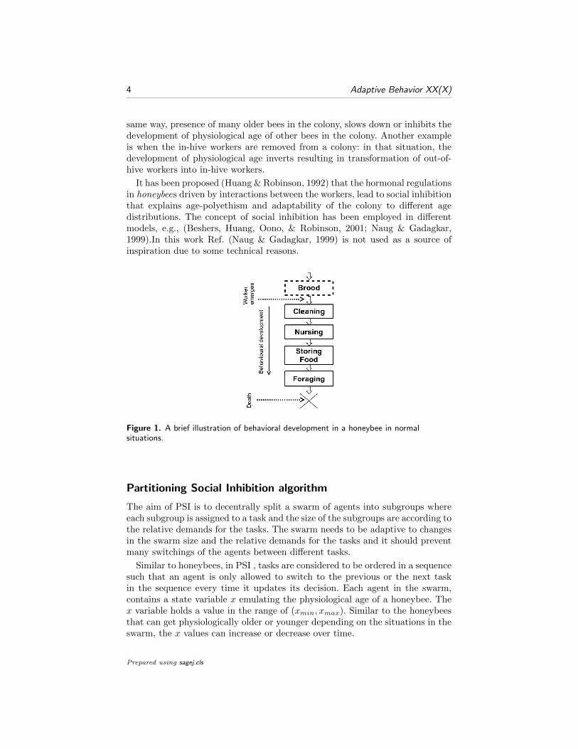
A worker honeybee goes through a behavioral development during its life-timetaking different tasks in different stages of its life. In a normal situation, ayoung worker honeybee starts with inside-hive tasks such as cleaning the comb.Then it grows older and undertakes tasks like nursing of the brood and storingfood. In some point in its life when the worker is old enough, it develops toan out-of-hive worker who performs foraging for nectar and pollen (Wilson,1971; Robinson, 1992; Johnson, 2010). Fig. 1 shows a brief illustration of thebehavioral development of a worker honeybee.

According to the task the worker undertakes, a number of morphological andphysiological changes occur in its body (Free & Spencer-Booth, 1959; Wilson,1971; N. Hrassnigg, 2005). This mechanism of behavioral development is calledage-polyethism (or temporal polyethism). In a normal situation, the tasks thatthe bee performs, and in turn, its so called physiological age, is correlated tothe chronological age of the bee (K. Crailsheim & Stabentheiner, 1996; Toth,Kantarovich, Meisel, & Robinson, 2005; Winston, 1987; Beshers, Robinson, &Mittenthal, 1999). This correlation can be violated though: The behavioraldevelopment can be delayed, accelerated, or even reversed in response to changesin the internal or environmental conditions of the colony. The adaptability ofthe colony to changes in the age-distribution and balance of the demands fordifferent tasks (Huang & Robinson, 1996) is a result of the adaptability in thebehavioral development. In a colony of mostly young honeybees, the age inwhich a bee starts foraging (which is a typical out-of-hive task) is lower than ina normal colony indicating acceleration in the behavioral development. In the

∗a short video that briefly describes the basic idea of the algorithm and experiments:https://youtu.be/ C7fFRSAW E



same way, presence of many older bees in the colony, slows down or inhibits thedevelopment of physiological age of other bees in the colony. Another exampleis when the in-hive workers are removed from a colony: in that situation, thedevelopment of physiological age inverts resulting in transformation of out-of-hive workers into in-hive workers.

It has been proposed (Huang & Robinson, 1992) that the hormonal regulationsin honeybees driven by interactions between the workers, lead to social inhibitionthat explains age-polyethism and adaptability of the colony to different agedistributions. The concept of social inhibition has been employed in differentmodels, e.g., (Beshers, Huang, Oono, & Robinson, 2001; Naug & Gadagkar,1999).In this work Ref. (Naug & Gadagkar, 1999) is not used as a source ofinspiration due to some technical reasons.

Figure 1. A brief illustration of behavioral development in a honeybee in normalsituations.

Partitioning Social Inhibition algorithm

The aim of PSI is to decentrally split a swarm of agents into subgroups whereeach subgroup is assigned to a task and the size of the subgroups are according tothe relative demands for the tasks. The swarm needs to be adaptive to changesin the swarm size and the relative demands for the tasks and it should preventmany switchings of the agents between different tasks.

Similar to honeybees, in PSI , tasks are considered to be ordered in a sequencesuch that an agent is only allowed to switch to the previous or the next taskin the sequence every time it updates its decision. Each agent in the swarm,contains a state variable x emulating the physiological age of a honeybee. Thex variable holds a value in the range of (xmin, xmax). Similar to the honeybeesthat can get physiologically older or younger depending on the situations in theswarm, the x values can increase or decrease over time.


5

The main idea of the algorithm is to dynamically distribute the x values ofthe swarm members over the fixed range of (xmin, xmax) via local interactionsand let the agents to choose their tasks based on their x values.

The (xmin, xmax) range is split into a number of segments, each of whichare associated with one of the tasks in the task sequence. An agent choosesa particular task if the value of its state variable (x) falls into the range ofthe segment associated with that task. Figure 2 represents an example swarmdivided into four task groups based on the state variables of its agents.

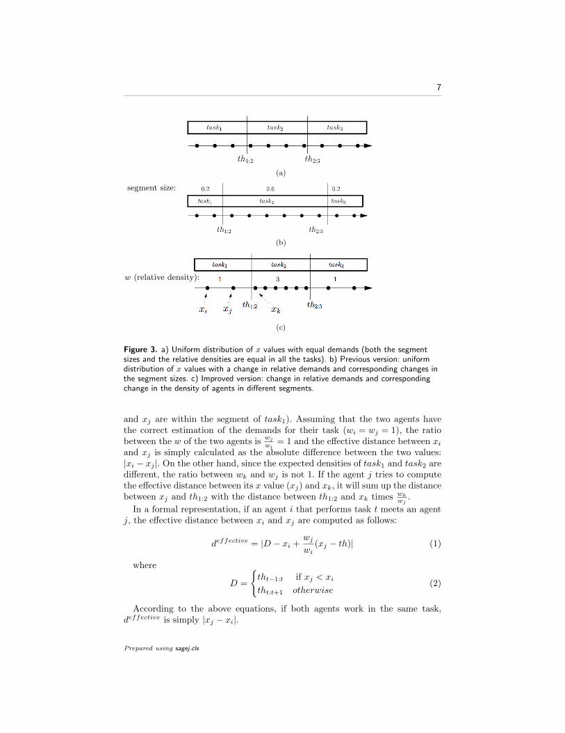
The distribution of the state variables over the range is uniform only if thedemands for all the tasks are equal. Otherwise, the density of the distributionis higher in the segments with higher associated task demands and lower inthe segments with lower associated task demands. Figure. 3(c) represents anexample of the distribution where there are different demands for the tasks.

In order to implement the idea of the algorithm, a set of thresholds are definedthat split the range (xmin, xmax) into the task segments. An agent chooses itstask based on its x value and the defined thresholds (see Fig. 2).

Figure 2. An example of uniform distribution of x values over the range of(xmin, xmax). Three threshold values (th1:2, th2:3, th3:4) split the range into foursegments associated with four different tasks. In this example, there is equal demand forall the tasks and the eight agents are divided into four groups of two agents each.

The thresholds are augmented with a lower and an upper margins. Thatmeans, an agent in taski switches to taski+1 if its x value exceeds thi:i+1 + lu.The agent switches to taski−1, if its x value becomes lower than thi−1:i − lb.The lower and upper margins prevent the agents from instant back and forthswitches between two consecutive tasks due to noise.

The aim is to divide the swarm into the task groups such that the numberof agents in different groups correlate with the demands for different tasks.In the preliminary version of the algorithm (Zahadat et al., 2013), this goalwas achieved by maintaining a uniform distribution of the x values in theswarm and using segments of different sizes, where the size of the segmentswere proportional to the demands for the tasks (See Fig. 3(b) for an example).The problem with that solution is that every change in the demand of a taskrequires changing of all the threshold values in the agents’ memories all over theswarm. This global information about the new values of the thresholds deviatesfrom the desire for distributiveness and was the main limitation of the previousalgorithm.

In the improved version of the algorithm, the problem is solved by keepingthe thresholds - and consequently the size of segments - fixed (e.g. to



equal segments), and instead, maintaining different densities in the segmentsproportional to the relative demands for the tasks (See Fig. 3(c)). In order todo that, each agent keeps a value w correlated to relative demand of its task.This value basically represents the expected relative density of agents in thattask. The w values are initially set by the user based on their initial assumptionsabout the relative demands for the tasks (e.g., set all to 1 for equal demands).The values can be changed by the agents according to their perception of thetask demands (for example, deviation from the assumed demands due to changesin the demands). The w values are used (along with other variables) to let theagents tune their x values (more details in the next subsection).

Fig. 3 shows an example comparing the previous and the improved versionsof the algorithm. In Fig. 3(a), the agents are distributed uniformly and thethresholds are set to split the range into equal segments due to equal demandfor the different tasks (both versions behave the same way in this case). Fig. 3(b)and Fig. 3(c) depict the results of a change in the relative demands of the tasks inthe previous version of the algorithm and the proposed version correspondingly.In Fig. 3(b), the distribution of the agents stays uniform after the change inthe demands from equal demands to higher demand for the task2. In that case,all the agents are globally informed to update their thresholds to new valuesaccording to the new demands for the tasks. Fig. 3(c) depicts the new versionof the algorithm where the thresholds stay constant but the changes in thedemands are reflected in the w of the agents in each task and lead to the changein the relative density of agents. In this case, for example, the relative demandfor task2 is three times as much as task1 (and task3) resulting in three times asmuch density in task2 as the density of agents in task1 (and task3).

By using the improved version of the algorithm, not only the adaptabilityto the changes in the swarm size (workforce) is maintained as in the previousversion, but also the local perception of the demands are automatically reflectedin the swarm by locally changing the w of the tasks within the agents and thereis no need for global information for updating the thresholds.

In the following, the implementation of the algorithm in the level of agents isdescribed.

PSI algorithm in the agent level

Since the agents have no global access to the status of the swarm, the x valuesof the agents change via local interactions with other agents over time. Inaddition to x and w, every agent needs to keep its own estimations of theeffective distances between its x value and the closest lower and higher x valuesof the other agents. The estimated effective distances, namely dlower and dhigher,change over time and during interactions with other agents and let the agentsto dynamically update their x values and consequently their choice of tasks.

When an agent meets another one, it receives the x and w of the other agent.The effective distance between the x values of the two agents is the distancebetween the two values while the ratio between the w of the two agents is takeninto account. For example, in Fig. 3(c), agents i and j are in the same task (xi


7

(a)

segment size:

(b)

w (relative density):

(c)

Figure 3. a) Uniform distribution of x values with equal demands (both the segmentsizes and the relative densities are equal in all the tasks). b) Previous version: uniformdistribution of x values with a change in relative demands and corresponding changes inthe segment sizes. c) Improved version: change in relative demands and correspondingchange in the density of agents in different segments.

and xj are within the segment of task1). Assuming that the two agents havethe correct estimation of the demands for their task (wi = wj = 1), the ratiobetween the w of the two agents is

wj

wi= 1 and the effective distance between xi

and xj is simply calculated as the absolute difference between the two values:|xi − xj |. On the other hand, since the expected densities of task1 and task2 aredifferent, the ratio between wk and wj is not 1. If the agent j tries to computethe effective distance between its x value (xj) and xk, it will sum up the distancebetween xj and th1:2 with the distance between th1:2 and xk times wk

wj.

In a formal representation, if an agent i that performs task t meets an agentj, the effective distance between xi and xj are computed as follows:

deffective = |D − xi +wj

wi(xj − th)| (1)

where

D =

{tht−1:t if xj < xi

tht:t+1 otherwise(2)

According to the above equations, if both agents work in the same task,deffective is simply |xj − xi|.



The estimated effective distances between xi and the closest lower and higherx values of the other agents (namely dlower

i and dhigheri ) get updated over timeand during interactions with other agents.

If an agent i meets an agent j, dloweri and dhigheri are updated based on their

current values and the effective distances between xi and xj ,as follows:

dloweri =

{deffective if xj < xi and deffective < dlower

i

dloweri otherwise

(3)

dhigheri =

{deffective if xi < xj and deffective < dhigheri

dhigheri otherwise(4)

Additionally, dloweri and dhigheri slowly increase in every step in order to be

adaptable to changes in x values of other agents as well as changes in theenvironmental conditions, i.e., changes in the workforce or task demands:

dloweri = dlower

i + ϕ

dhigheri = dhigheri + ϕ(5)

where ϕ is a small value in terms of segments sizes.

Fig. 4 depicts an example update of dlower and dhigher after receiving datafrom another agent.

Every agent tends to keep its x value equally distanced from the closest higherand lower x values of the others. Therefore, with every update of the dlower anddhigher, the x value is also updated, as follows:

x =

x+ δ if dlower < dhigher

x− δ if dlower > dhigher

x±X otherwise

(6)

where δ is step-size which is a constant parameter with a small value in termsof the size of task segments. In the current implementation X ∼ δ × U(0, 1).

After every update of x, an agent considers switching to the previous or thenext tasks in the task sequence. For an agent in taskt, new task is chosen asfollows:

new task =

taskt+1 if x > tht:t+1 + lu

taskt−1 if x < tht−1:t − lbtaskt otherwise

(7)

where tht−1:t and tht:t+1 represent the threshold values between taskt−1 andtaskt, and taskt and taskt+1 respectively. lu and lb are the upper and lowermargins for the thresholds.


9

(a) An agent receives data from another agent.

(b) The dhigher gets updated according to the

value received from the other agent.

(c) The dhigher and dlower slowly increase inevery step.

Figure 4. An example of dlower and dhigher getting updated via interaction with anotheragent. For clarity of the example, the two agents in (a) are assumed to work in the sametask (therefore the effective distance between the two x values is simply the absolutedifference between them).

Summarizing the PSI algorithm The following actions are performed by anyagent i that receives information from another agent j:

1. update dlower and dhigher using Eq. 5.2. update x using Eq. 6.3. update dlower and dhigher using Eq. 3 and Eq. 4.4. update the assigned task using Eq. 7.

A heuristic used for updating delta-window (ϕ) In the robotic experimentsreported in this paper, we applied the following heuristic to regulate ϕ based onthe periods between the interactions for every agent. The value of ϕ is updatedfor an agent every time it receives information from another agents, as follows:

ϕ = ϕbase/(T + 1)

T = (1− α)× T + α ∗ Tlast(8)

where α = 0.1, and Tlast is the time (number of time-steps) since the lastinteraction occurred. ϕbase is a constant parameter.



Experimenting in simulation

The proposed algorithm is preliminarily tested in an agent-based spatialsimulation without embodiment.

First, two sets of experiments are performed in order to investigate theadaptability of the swarm to changes in the total number of available agentsand the demands for different tasks. Then, several experiments with differentswarm sizes and communication ranges are performed in order to give a betterunderstanding of the performance of the algorithm in different setups.

The agents are located in a column with different horizontal layers associatedwith different tasks (similar to the robotic experiment in Fig.9) and they have alimited range of communication. The agents randomly drift around in their tasklayers with the average speed of 2cm/sec while every 7 times-steps considers asone second.

All the agents start with an identical initial x value belonging to task1.The range of x values is split into five equal segments by setting up thethresholds (th1:2 to th4:5) accordingly. In every time-step, each agent is allowedto communicate with a randomly chosen agent in its communication range. Inall the following experiments, we assume that the agents can precisely estimatethe relative demands for the tasks they perform.

All the experiments are repeated for 25 independent runs. The experimentalsettings of the algorithm are represented in Table 1.

The performance of the swarms are measured in the experiments by usingtwo metrics: number of errors and number of switchings. The number of errorsrepresent the difference between the required and actual number of agents inevery task for all the tasks in total. The number of switchings is the number ofunintended changes in the choice for the tasks counted over the whole swarm ina fixed period of time.

Table 1. Parameter settings of the algorithm for simulation and robot experiments

simulation robotxmin 0 0xmax 1024 214 − 1noise on x 0 0.5δ 1 70ϕbase 0.3 210lu, lb 3 140thresholds equal segments equal segmentsinitial x 2 thr1:2 − 20initial dlower x− xmin − 1 x− xmin − 10initial dhigher xmax − x− 1 xmax − x− 10

Adaptivity to changes in workforce

In the first set of experiments, the swarm is expected to take care of five taskslocated in five different layers. The size of each layer is 40× 40cm2 and the


11

distance between the layers is 35cm. The communication range is 50cm. Eachrun, continues for 70,000 time-steps.

In this set of experiments, there are equal demands for all the five tasks andthe demands stay constant during the runs. The number of available agents is30 in the beginning. The number of agents is then suddenly changed at twopoints of time during the runtime and the swarm is supposed to react to thechanges by rearranging the agents in the tasks according to the new conditions.

The agents start in task1 with initially identical x values which they regulategradually via interactions with other agents. After some time, the x values areequally distributed in the swarm leading to the equal number of robots in eachtask due to the equal segmentation of the range by the task thresholds.

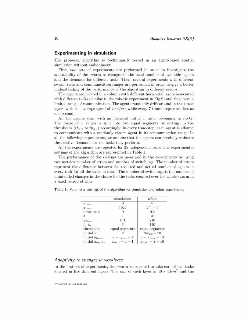
Fig. 5(a) represents the number of agents in each task (median from25 independent runs) and Fig. 5(b) represents the total number of agentspositioning in a wrong task according to the desired number of agents in thetasks.

In time-step 20,000, all the agents working in task3 and task4 are removedfrom the swarm. The swarm reacts to this deviation from uniformity of thedistribution of x values, by shifting the x values of the remaining agents andends up to a new equal number of agents (three agents) in each task.

In time-step 40,000, 12 agents are added to the swarm in task3. For that, theinitial x value of the new agents are set to the average of the two thresholdsseparating task3 from its neighboring tasks (th2:3 and th3:4). The swarm reactsto this change by regulating the x values for the new situation and after a while,six agents are assigned to each task.

Adaptivity to changes in demands

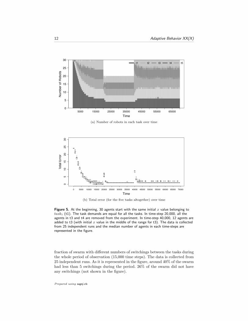
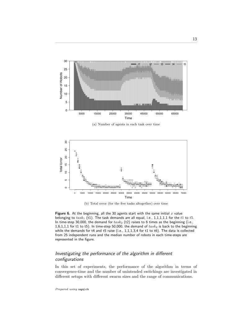
The adaptability of the swarm to the changes in the demands is investigatedin this experiments. The swarm size is 30 and the number of tasks and spatialconfigurations are the same as in the previous section. The demands are equalfor the five tasks in the beginning until time-step 30, 000. The agents start intask1 and after a while they equally distribute in the five tasks.

Fig. 6(a) represents the number of agents in each task during the simulationperiod (median from 25 independent runs). At time-step 30, 000, the demandschange such that the demand for task2 suddenly raises to 6 times as much asthe starting demand. The new relative demands are considered as 1,6,1,1,1 fortask1 to task5 accordingly. At time-step 50, 000, the relative demands changeabruptly again to 1,1,1,3,4 for task1 to task5 accordingly. Fig. 6(b) representsthe total number of agents performing a wrong task.

Number of switchings between tasks

The number of unintended switchings (switching to a wrong task) are countedin the period between 15,000 and 30,000 time-steps with the same settingsas the previous experiment (Fig. 6). The period is chosen since there is noexternal disturbance on the system in this period meaning that in an optimalcase there should be no switchings between the layers. Fig. 7 represents the



Time

Num

ber

of R

obots

0

5

10

15

20

25

30

5000 15000 25000 35000 45000 55000 65000

t1 t2 t3 t4 t5

(a) Number of robots in each task over time

Time

Tota

l E

rror

0 5000 10000 15000 20000 25000 30000 35000 40000 45000 50000 55000 60000 65000 70000

05

10

15

20

25

30

(b) Total error (for the five tasks altogether) over time

Figure 5. At the beginning, 30 agents start with the same initial x value belonging totask1 (t1). The task demands are equal for all the tasks. In time-step 20,000, all theagents in t3 and t4 are removed from the experiment. In time-step 40,000, 12 agents areadded to t3 (with initial x value in the middle of the range for t3). The data is collectedfrom 25 independent runs and the median number of agents in each time-steps arerepresented in the figure.

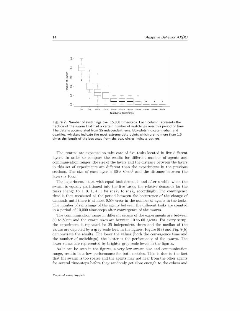
fraction of swarm with different numbers of switchings between the tasks duringthe whole period of observation (15,000 time steps). The data is collected from25 independent runs. As it is represented in the figure, around 40% of the swarmhad less than 5 switchings during the period. 26% of the swarm did not haveany switchings (not shown in the figure).


13

Time

Num

ber

of R

obots

0

5

10

15

20

25

30

5000 15000 25000 35000 45000 55000 65000

t1 t2 t3 t4 t5

(a) Number of agents in each task over time

Time

Tota

l E

rror

0 5000 10000 15000 20000 25000 30000 35000 40000 45000 50000 55000 60000 65000 70000

05

10

15

20

25

30

(b) Total error (for the five tasks altogether) over time

Figure 6. At the beginning, all the 30 agents start with the same initial x valuebelonging to task1 (t1). The task demands are all equal, i.e., 1,1,1,1,1 for the t1 to t5.In time-step 30,000, the demand for task2 (t2) raises to 6 times as the beginning (i.e.,1,6,1,1,1 for t1 to t5). In time-step 50,000, the demand of task2 is back to the beginningwhile the demands for t4 and t5 raise (i.e., 1,1,1,3,4 for t1 to t6). The data is collectedfrom 25 independent runs and the median number of robots in each time-steps arerepresented in the figure.

Investigating the performance of the algorithm in differentconfigurations

In this set of experiments, the performance of the algorithm in terms ofconvergence-time and the number of unintended switchings are investigated indifferent setups with different swarm sizes and the range of communications.



Number of Switchings

Fra

ction o

f S

warm

0−4 5−9 10−14 15−19 20−24 25−29 30−34 35−39 40−44 45−49 50−54

0.0

0.1

0.2

0.3

0.4

0.5

Figure 7. Number of switchings over 15,000 time-steps. Each column represents thefraction of the swarm that had a certain number of switchings over this period of time.The data is accumulated from 25 independent runs. Box-plots indicate median andquartiles, whiskers indicate the most extreme data points which are no more than 1.5times the length of the box away from the box, circles indicate outliers.

The swarms are expected to take care of five tasks located in five differentlayers. In order to compare the results for different number of agents andcommunication ranges, the size of the layers and the distance between the layersin this set of experiments are different than the experiments in the previoussections. The size of each layer is 80× 80cm2 and the distance between thelayers is 10cm.

The experiments start with equal task demands and after a while when theswarm is equally partitioned into the five tasks, the relative demands for thetasks change to 1, 3, 1, 4, 1 for task1 to task5 accordingly. The convergencetime is then measured as the period between the occurrence of the change ofdemands until there is at most 0.5% error in the number of agents in the tasks.The number of switchings of the agents between the different tasks are countedin a period of 10,000 time-steps after convergence of the swarm.

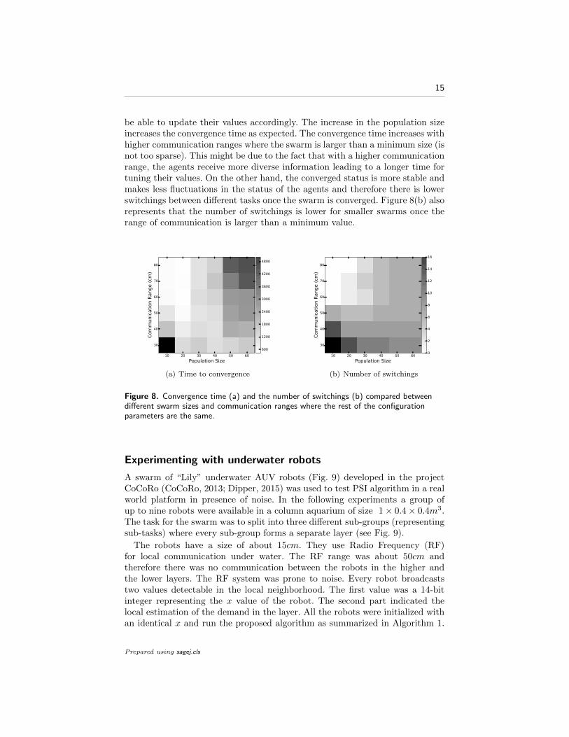
The communication range in different setups of the experiments are between30 to 80cm and the swarm sizes are between 10 to 60 agents. For every setup,the experiment is repeated for 25 independent times and the median of thevalues are depicted by a grey scale level in the figures. Figure 8(a) and Fig. 8(b)demonstrate the results. The lower the values (both the convergence time andthe number of switchings), the better is the performance of the swarm. Thelower values are represented by brighter grey scale levels in the figures.

As it can be seen in the figures, a very low swarm size and communicationrange, results in a low performance for both metrics. This is due to the factthat the swarm is too sparse and the agents may not hear from the other agentsfor several time-steps before they randomly get close enough to the others and


15

be able to update their values accordingly. The increase in the population sizeincreases the convergence time as expected. The convergence time increases withhigher communication ranges where the swarm is larger than a minimum size (isnot too sparse). This might be due to the fact that with a higher communicationrange, the agents receive more diverse information leading to a longer time fortuning their values. On the other hand, the converged status is more stable andmakes less fluctuations in the status of the agents and therefore there is lowerswitchings between different tasks once the swarm is converged. Figure 8(b) alsorepresents that the number of switchings is lower for smaller swarms once therange of communication is larger than a minimum value.

10 20 30 40 50 60

Population Size

80

70

60

50

40

30

Communication Range (cm

)

600

1200

1800

2400

3000

3600

4200

4800

(a) Time to convergence

10 20 30 40 50 60

Population Size

80

70

60

50

40

30

Communication Range (cm

)

0

2

4

6

8

10

12

14

16

(b) Number of switchings

Figure 8. Convergence time (a) and the number of switchings (b) compared betweendifferent swarm sizes and communication ranges where the rest of the configurationparameters are the same.

Experimenting with underwater robots

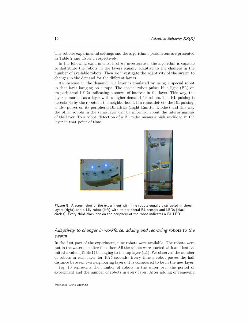
A swarm of “Lily” underwater AUV robots (Fig. 9) developed in the projectCoCoRo (CoCoRo, 2013; Dipper, 2015) was used to test PSI algorithm in a realworld platform in presence of noise. In the following experiments a group ofup to nine robots were available in a column aquarium of size 1× 0.4× 0.4m3.The task for the swarm was to split into three different sub-groups (representingsub-tasks) where every sub-group forms a separate layer (see Fig. 9).

The robots have a size of about 15cm. They use Radio Frequency (RF)for local communication under water. The RF range was about 50cm andtherefore there was no communication between the robots in the higher andthe lower layers. The RF system was prone to noise. Every robot broadcaststwo values detectable in the local neighborhood. The first value was a 14-bitinteger representing the x value of the robot. The second part indicated thelocal estimation of the demand in the layer. All the robots were initialized withan identical x and run the proposed algorithm as summarized in Algorithm 1.



The robotic experimental settings and the algorithmic parameters are presentedin Table 2 and Table 1 respectively.

In the following experiments, first we investigate if the algorithm is capableto distribute the robots in the layers equally adaptive to the changes in thenumber of available robots. Then we investigate the adaptivity of the swarm tochanges in the demand for the different layers.

An increase in the demand in a layer is emulated by using a special robotin that layer hanging on a rope. The special robot pulses blue light (BL) onits peripheral LEDs indicating a source of interest in the layer. This way, thelayer is marked as a layer with a higher demand for robots. The BL pulsing isdetectable by the robots in the neighborhood. If a robot detects the BL pulsing,it also pulses on its peripheral BL LEDs (Light Emitter Diodes) and this waythe other robots in the same layer can be informed about the interestingnessof the layer. To a robot, detection of a BL pulse means a high workload in thelayer in that point of time.

Figure 9. A screen-shot of the experiment with nine robots equally distributed in threelayers (right) and a Lily robot (left) with its peripheral BL sensors and LEDs (blackcircles). Every third black dot on the periphery of the robot indicates a BL LED.

Adaptivity to changes in workforce: adding and removing robots to theswarm

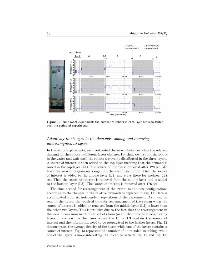
In the first part of the experiment, nine robots were available. The robots wereput in the water one after the other. All the robots were started with an identicalinitial x value (Table 1) belonging to the top layer (L1). We observed the numberof robots in each layer for 1025 seconds. Every time a robot passes the halfdistance between two neighboring layers, it is considered to be in the new layer.

Fig. 10 represents the number of robots in the water over the period ofexperiment and the number of robots in every layer. After adding or removing


17

Algorithm 1 robots’ operational loop

while true doif data available from other robots ∗ then

update dlower and dhigher by Eq. 3 and 4end ifupdate x value by Eq. 6increase dlower and dhigher by Eq. 5broadcast data (x, w)choose a layer based on x value by Eq. 7if new layer is different than the current layer then

change the target depth to the new layerend ifif detect the high demand signal then

set the w to a high valueemit BL pulse (high demand signal)

elseset the w to a low value

end ifend while∗at most, one set of data can be accepted in every cycle due to limitations in therobot’s operation.

a robot, the swarm rearranges to a new configuration close to the status wherethe number of robots in all layers are equal. In the beginning, the robots areadded to the swarm one after the other until six robots are in the water. Theswarm forms a three-layers configuration with two robots in each layer. Weleave the swarm for 270sec during which no switching of the robots betweenthe layers occur. After this period, three more robots are added to the swarmresulting in switching of some of the robots to new layers such that there isthree robots in each layer. In the period between the first appearance of the newconfiguration and before making a new change in the swarm size (at 690sec),three unintended switchings (switching to a wrong layer) occurs. In second 690,all the three robots in the top layer (L1) are removed from the water almostat the same time. The swarm then rearranges such that each layer keeps tworobots. This configuration stays until a new change in the swarm size is enforcedby the experimenter. In second 950, the two robots in the top layer (L1) andone robot from the middle layer (L2) are removed. The three remaining robotsrelocate such that every layer contains a single robots. Table 3 represents theaverage density of robots in every layer over the experiment period and thenumber of unintended switchings between the layers.



Figure 10. Nine robot experiment: the number of robots in each layer are representedover the period of experiment.

Adaptivity to changes in the demands: adding and removinginterestingness to layers

In this set of experiments, we investigated the swarm behavior when the relativedemand for the robots in different layers changes. For that, we first put six robotsin the water and wait until the robots are evenly distributed in the three layers.A source of interest is then added to the top layer meaning that the demand israised in the top layer (L1). The source of interest is removed after 128 sec. Weleave the swarm to again rearrange into the even distribution. Then the sourceof interest is added to the middle layer (L2) and stays there for another 128sec. Then the source of interest is removed from the middle layer and is addedto the bottom layer (L3). The source of interest is removed after 176 sec.

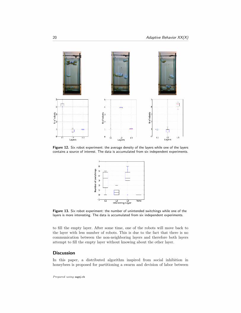
The time needed for rearrangement of the swarm to the new configurationsaccording to the changes in the relative demands is depicted in Fig. 11. Data isaccumulated from six independent repetitions of the experiment. As it can beseen in the figure, the required time for rearrangement of the swarm when thesource of interest is added or removed from the middle layer (L2) is lower thanthe other two layers. This is intuitive due to the fact that the rearrangement inthis case means movement of the robots from (or to) the immediate neighboringlayers in contrast to the cases where the L1 or L3 contain the source ofinterest and the information need to be propagated to the farther layers. Fig. 12demonstrates the average density of the layers while one of the layers contains asource of interest. Fig. 13 represents the number of unintended switchings whileone of the layers is more interesting. As it can be seen in Fig. 12 and Fig. 13,


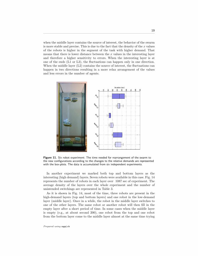
19

when the middle layer contains the source of interest, the behavior of the swarmis more stable and precise. This is due to the fact that the density of the x valuesof the robots is higher in the segment of the task with higher demand. Thatmeans that there is lower distance between the x values in the interesting layerand therefore a higher sensitivity to errors. When the interesting layer is atone of the ends (L1 or L3), the fluctuations can happen only in one direction.When the middle layer (L2) contains the source of interest, the fluctuations canhappen in two directions resulting in a more relax arrangement of the valuesand less errors in the number of agents.

Figure 11. Six robot experiment: The time needed for rearrangement of the swarm tothe new configurations according to the changes to the relative demands are representedwith the box-plots. The data is accumulated from six independent experiments.

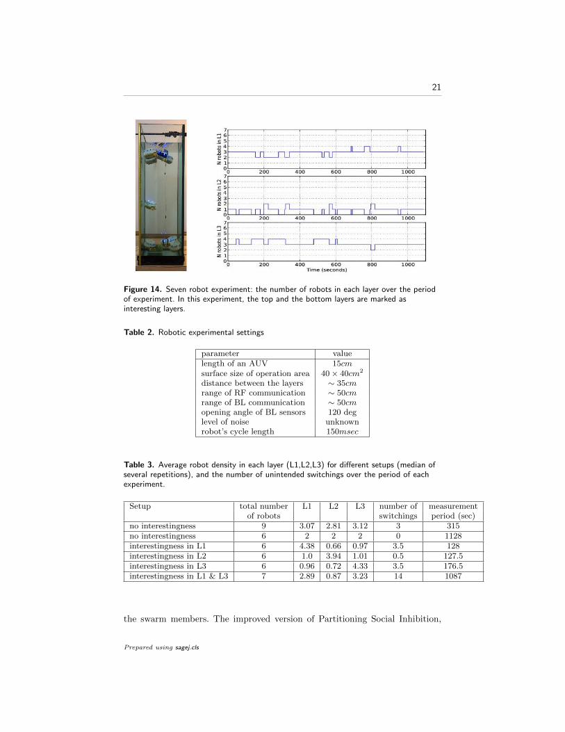
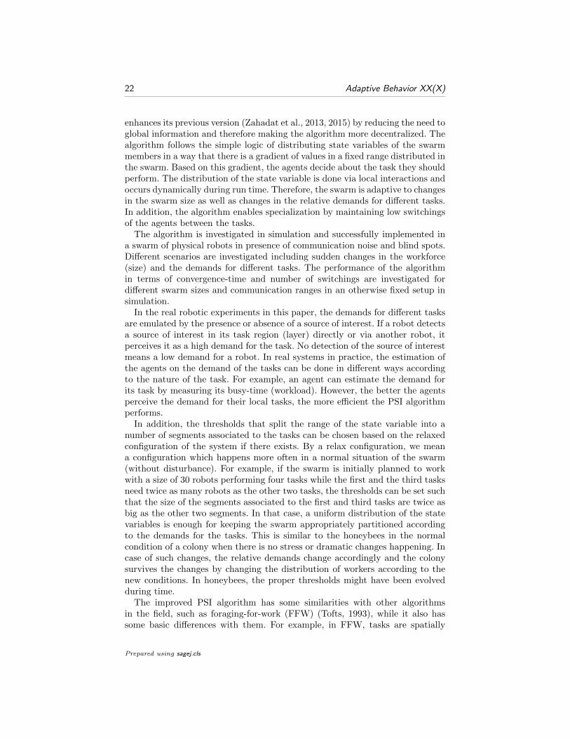
In another experiment we marked both top and bottom layers as theinteresting (high demand) layers. Seven robots were available in this case. Fig. 14represents the number of robots in each layer over 1087 sec of experiment. Theaverage density of the layers over the whole experiment and the number ofunintended switchings are represented in Table 3.

As it is shown in Fig. 14, most of the time, three robots are present in thehigh-demand layers (top and bottom layers) and one robot in the low-demandlayer (middle layer). Once in a while, the robot in the middle layer switches toone of the other layers. The same robot or another robot will then fill in theempty layer after a short period of time. In some cases when the middle layeris empty (e.g., at about second 200), one robot from the top and one robotfrom the bottom layer come to the middle layer almost at the same time trying



Figure 12. Six robot experiment: the average density of the layers while one of the layerscontains a source of interest. The data is accumulated from six independent experiments.

Figure 13. Six robot experiment: the number of unintended switchings while one of thelayers is more interesting. The data is accumulated from six independent experiments.

to fill the empty layer. After some time, one of the robots will move back tothe layer with less number of robots. This is due to the fact that there is nocommunication between the non-neighboring layers and therefore both layersattempt to fill the empty layer without knowing about the other layer.

Discussion

In this paper, a distributed algorithm inspired from social inhibition inhoneybees is proposed for partitioning a swarm and devision of labor between


21

Figure 14. Seven robot experiment: the number of robots in each layer over the periodof experiment. In this experiment, the top and the bottom layers are marked asinteresting layers.

Table 2. Robotic experimental settings

parameter valuelength of an AUV 15cmsurface size of operation area 40× 40cm2

distance between the layers ∼ 35cmrange of RF communication ∼ 50cmrange of BL communication ∼ 50cmopening angle of BL sensors 120 deglevel of noise unknownrobot’s cycle length 150msec

Table 3. Average robot density in each layer (L1,L2,L3) for different setups (median ofseveral repetitions), and the number of unintended switchings over the period of eachexperiment.

Setup total number L1 L2 L3 number of measurementof robots switchings period (sec)

no interestingness 9 3.07 2.81 3.12 3 315no interestingness 6 2 2 2 0 1128interestingness in L1 6 4.38 0.66 0.97 3.5 128interestingness in L2 6 1.0 3.94 1.01 0.5 127.5interestingness in L3 6 0.96 0.72 4.33 3.5 176.5interestingness in L1 & L3 7 2.89 0.87 3.23 14 1087

the swarm members. The improved version of Partitioning Social Inhibition,



enhances its previous version (Zahadat et al., 2013, 2015) by reducing the need toglobal information and therefore making the algorithm more decentralized. Thealgorithm follows the simple logic of distributing state variables of the swarmmembers in a way that there is a gradient of values in a fixed range distributed inthe swarm. Based on this gradient, the agents decide about the task they shouldperform. The distribution of the state variable is done via local interactions andoccurs dynamically during run time. Therefore, the swarm is adaptive to changesin the swarm size as well as changes in the relative demands for different tasks.In addition, the algorithm enables specialization by maintaining low switchingsof the agents between the tasks.

The algorithm is investigated in simulation and successfully implemented ina swarm of physical robots in presence of communication noise and blind spots.Different scenarios are investigated including sudden changes in the workforce(size) and the demands for different tasks. The performance of the algorithmin terms of convergence-time and number of switchings are investigated fordifferent swarm sizes and communication ranges in an otherwise fixed setup insimulation.

In the real robotic experiments in this paper, the demands for different tasksare emulated by the presence or absence of a source of interest. If a robot detectsa source of interest in its task region (layer) directly or via another robot, itperceives it as a high demand for the task. No detection of the source of interestmeans a low demand for a robot. In real systems in practice, the estimation ofthe agents on the demand of the tasks can be done in different ways accordingto the nature of the task. For example, an agent can estimate the demand forits task by measuring its busy-time (workload). However, the better the agentsperceive the demand for their local tasks, the more efficient the PSI algorithmperforms.

In addition, the thresholds that split the range of the state variable into anumber of segments associated to the tasks can be chosen based on the relaxedconfiguration of the system if there exists. By a relax configuration, we meana configuration which happens more often in a normal situation of the swarm(without disturbance). For example, if the swarm is initially planned to workwith a size of 30 robots performing four tasks while the first and the third tasksneed twice as many robots as the other two tasks, the thresholds can be set suchthat the size of the segments associated to the first and third tasks are twice asbig as the other two segments. In that case, a uniform distribution of the statevariables is enough for keeping the swarm appropriately partitioned accordingto the demands for the tasks. This is similar to the honeybees in the normalcondition of a colony when there is no stress or dramatic changes happening. Incase of such changes, the relative demands change accordingly and the colonysurvives the changes by changing the distribution of workers according to thenew conditions. In honeybees, the proper thresholds might have been evolvedduring time.

The improved PSI algorithm has some similarities with other algorithmsin the field, such as foraging-for-work (FFW) (Tofts, 1993), while it also hassome basic differences with them. For example, in FFW, tasks are spatially


23

arranged in a sequence and agents wander around and seek a task to perform.The spatial presence and physical movement of the agents in the task areaslead to the distribution of the agents relative to the task demands. In PSI,instead of physical spatial positioning of the agents, the physiological age (x)of the agents is virtually distributed relative to the task demands and leads tophysical distribution of the agents in different areas. From a biological pointof view, FFW does not consider physiological differences between bees to drivethem to perform different tasks. On the contrary, in PSI, a physiological age (x)is defined for the agents in an analogy to the physiological and morphologicalcharacteristics of the agents. There are also other methods such as stochasticpolicies as discussed in (Berman, Halasz, Hsieh, & Kumar, 2009). That methoddoes not assume sequential ordering of the tasks. Instead, it uses a directedgraph that defines interconnection topology of possible switchings between thetasks. Unlike PSI that aims for low task switchings, the stochastic policy methodworks based on persistent transitions between tasks while the transition ratesare computed according to the demand for different tasks. The low switchingrate of PSI, leads to lower time and energy costs in the swarm and enables theagents to specialize in their tasks.

In the future, we will study the behavior of the algorithm in more practicalphysical scenarios where the robots actually fullfil some real works.

Acknowledgements This work is supported by: EU-ICT project ‘CoCoRo’,no. 270382; EU-H2020 project ‘subCULTron’, no. 640967;

References

Berman, S., Halasz, A., Hsieh, M. A., & Kumar, V. (2009). Optimizedstochastic policies for task allocation in swarms of robots. Robotics, IEEETransactions on, 25 (4), 927–937.

Beshers, S., & Fewell, J. (2001). Models of division of labor in social insects.Annu. Rev. Entomol , 46 , 413-440.

Beshers, S., Huang, Z., Oono, Y., & Robinson, G. (2001). Social inhibitionand the regulation of temporal polyethism in honey bees. Journal ofTheoretical Biology , 213 (3), 461-479.

Beshers, S., Robinson, G., & Mittenthal, J. (1999). Response thresholds anddivision of labor in social insects. In C. Detrain, J. Deneubourg, &J. Pasteels (Eds.), Information processing in social insects (p. 115-139).Basel: Birkhauser.

Bonabeau, E., Sobkowski, A., Theraulaz, G., & Deneubourg, J.-L. (1997).Adaptive task allocation inspired by a model of division of labor in socialinsects. In Biocomputing and emergent computation: Proceedings of bcec97(pp. 36–45). World Scientific Press.

CoCoRo. (2013). Project website. (http://cocoro.uni-graz.at)Crosland, M. W. J., Ren, S. X., & Traniello, J. F. A. (2010). Division of

labour among workers in the termite, reticulitermes fukienensis (isoptera:Rhinotermitidae). Ethology , 104 , 57-67.



Dipper, T. (2015). Einsatz von elektrischen Feldern zur Lokalisierungvon autonomen Unterwasserschwarmrobotern (Unpublished doctoraldissertation). University of Stuttgart. (in: BV-Forschungsberichte)

Ferrante, E., Turgut, A. E., Duez-Guzmn, E. A., Dorigo, M., & Wenseleers, T.(2015). Evolution of self-organized task specialization in robot swarms.PLoS Computational Biology , 11 (8), e1004273.

Free, J. B., & Spencer-Booth, Y. (1959). The longevity of worker honeybees.Proceedings of the Royal Entomological Society of London. Series A,General Entomology , 34 (10-12), 141-150. doi: 10.1111/j.1365-3032.1959.tb00230.x

Gross, R., Nouyan, S., Bonani, M., Mondada, F., & Dorigo, M. (2008). Divisionof labour in self-organised groups. In Sab (p. 426-436). Berlin, Heidelberg:Springer Berlin Heidelberg.

Holldobler, B., & Wilson, E. (2008). The superorganism: The beauty, elegance,and strangeness of insect societies. New York: W. W. Norton andCompany.

Huang, Z.-Y., & Robinson, G. (1999). Social control of division of labor inhoney bee colonies. In C. Detrain, J. Deneubourg, & J. Pasteels (Eds.),Information processing in social insects (p. 165-186). Basel: Birkhauser.

Huang, Z. Y., & Robinson, G. E. (1992). Honeybee colony integration: worker-worker interactions mediate hormonally regulated plasticity in division oflabor. Proc Natl Acad Sci U S A, 89 (24), 11726-9.

Huang, Z. Y., & Robinson, G. E. (1996). Regulation of honey bee division oflabor by colony age demography. Behavioral Ecology and Sociobiology ,39 (3), 147-158.

Johnson, B. (2010, January). Division of labor in honeybees: form, function,and proximate mechanisms. Behavioral Ecology and Sociobiology , 64 (3),305–316.

Jones, C., & Mataric, M. J. (2003). Adaptive division of labor in large-scaleminimalist multi-robot systems. In Ieee/rsj international conference onintelligent robots and systems (iros) (p. 1969-1974). Las Vegas, Nevada:IEEE.

Julian, G. E., & Cahan, S. (1999). Undertaking specialization in the desertleaf-cutter ant acromyrmex versicolor. Anim Behav , 58 (2), 437-442.

Karsai, I., & Schmickl, T. (2011). Regulation of task partitioning by a ”commonstomach”: a model of nest construction in social wasps. BehavioralEcology , 22 , 819-830. doi: 10.1093/beheco/arr060

K. Crailsheim, N. H., & Stabentheiner, A. (1996). Diurnal behaviouraldifferences in forager and nurse honey bees (apis mellifera carnica pollm).Apidologie, 27 (4), 235-244. doi: 10.1051/apido:19960406

Labella, T. H., Dorigo, M., & Deneubourg, J.-L. (2006, September). Divisionof labor in a group of robots inspired by ants’ foraging behavior. ACMTrans. Auton. Adapt. Syst., 1 (1), 4–25.

Naug, D., & Gadagkar, R. (1999). Flexible division of labor mediated by socialinteractions in an insect colony a simulation model. Journal of TheoreticalBiology , 197 , 123-133.


25

Navarro, I., & Matıa, F. (2013). An introduction to swarm robotics. ISRNRobotics, 2013 , 608164.

N. Hrassnigg, K. C. (2005). Differences in drone and worker physiology inhoneybees (apis mellifera). Apidologie, 36 (2), 255 - 277. doi: 10.1051/apido:2005015

Robinson, G. E. (1992). Regulation of division of labor in insect societies. AnnuRev Entomol , 37 , 637-65.

Sahin, E. (2005). Swarm robotics: From sources of inspiration to domains ofapplication. In Lecture notes in computer science (Vol. 3342, p. 10-20).Berlin, Germany: Springer-Verlag.

Schmickl, T., Moslinger, C., & Crailsheim, K. (2007). Collective perceptionin a robot swarm. In E. Sahin, W. M. Spears, & A. F. T. Winfield(Eds.), Swarm robotics - second sab 2006 international workshop (Vol.4433). Heidelberg/Berlin, Germany: Springer-Verlag.

Seeley, T. D. (1982). Adaptive significance of the age polyethism schedule inhoneybee colonies. Behavioral Ecology and Sociobiology , 11 , 287-293.

Theraulaz, G., Bonabeau, E., & Deneubourg, J.-L. (1998). Response thresholdreinforcement and division of labour in insect societies. Proceedings of theRoyal Society of London B: Biological Sciences, 265 (1393), 327- 332.

Tofts, C. (1993). Algorithms for task allocation in ants. Bull. Math. Biol., 55 ,891-918.

Torres, V., Montagna, T., Raizer, J., & Antonialli-Junior, W. (2012). Division oflabor in colonies of the eusocial wasp, mischocyttarus consimilis. Journalof insect science, 12 , 21. doi: 10.1673/031.012.2101

Toth, A. L., Kantarovich, S., Meisel, A. F., & Robinson, G. E. (2005).Nutritional status influences socially regulated foraging ontogeny in honeybees. The Journal of experimental biology , 208 , 4641-4649.

White, T., & Helferty, J. (2005). Emergent Team Formation: Applying Divisionof Labour Principles to Robot Soccer. Engineering Self-OrganisingSystems, 180–194.

Wilson, E. O. (1971). The insect societies. Cambridge, MA: Belknap Press ofHarvard University Press.

Winston, M. (1987). The biology of the honey bee. Cambridge, MA: HarvardUniversity Press.

Yang, Y., Zhou, C., & Tian, Y. (2009). Swarm robots task allocation based onresponse threshold model. In G. S. Gupta & S. C. Mukhopadhyay (Eds.),Icara (p. 171-176). Wellington: IEEE.

Zahadat, P., Crailsheim, K., & Schmickl, T. (2013). Social inhibition managesdivision of labour in artificial swarm systems. In P. Lio, O. Miglino,G. Nicosia, S. Nolfi, & M. Pavone (Eds.), 12th european conference onartificial life (ecal 2013) (p. 609-616). MIT Press. doi: http://dx.doi.org/10.7551/978-0-262-31709-2-ch087

Zahadat, P., Hahshold, S., Thenius, R., Crailsheim, K., & Schmickl, T.(2015). From honeybees to robots and back: Division of labor basedon partitioning social inhibition. Bioinspiration & Biomimetics, 10 (6),066005. doi: 10.1088/1748-3190/10/6/066005


adaptive behavior division of labor in a swarm of...

Documents