adaptive filtering algorithms for noise … filtering algorithms for noise cancellation ... the...
TRANSCRIPT

Faculdade de Engenharia da Universidade do Porto
ADAPTIVE FILTERING ALGORITHMS FOR NOISE CANCELLATION
Rafael Merredin Alves Falcão
Dissertação realizada no âmbito do Mestrado Integrado em Engenharia Electrotécnica e de Computadores
Major Automação
Orientador: Rodrigo Caiado de Lamare (Doutor) Coorientador: Rui Esteves Araújo (Doutor)
Julho de 2012

© Rafael Merredin Alves Falcão, 2012

i
Abstract
The purpose of this thesis is to study the adaptive filters theory for the noise cancellation
problem. Firstly the paper presents the theory behind the adaptive filters. Secondly it
describes three most commonly adaptive filters which were also used in computer
experiments, the LMS, NLMS and RLS algorithms. Furthermore, the study explains some of the
applications of adaptive filters, the system identification and prediction problems. It also
describes some computer experiments conducted by the author within a general problem,
providing its solution by using the LMS, NLMS and the RLS algorithms and comparing the
results. Moreover, the work focuses on one of the classes of application of the adaptive
filters: the active noise cancellation problem, presenting a general problem, the three
different algorithm solutions and a comparison between them. The study continues giving a
simulation of a specific problem of noise cancellation in speech signal, using Simulink
platform in two different environments. The first one uses a white Gaussian as the noise
signal and the second uses a colored noise signal. To solve this problem, both LMS and RLS
algorithms were used and results of their applications are being presented in further part of
this work. The investigation ends with choosing the best solution to this specific problem and
discussing possibilities for future research.

ii

iii
Resumo
Este trabalho foi elaborado com o intuito de estudar a teoria dos filtros adaptativos
aplicados ao problema de cancelamento de ruído. Primeiramente o trabalho revê a teoria dos
filtros adaptativos. Em seguida, descrevem-se três algoritmos muito utilizados: LMS (least-
mean square), NLMS (normalized least-mean square) e RLS (recursive least square). Mais
adiante, esse estudo explica algumas das aplicações dos filtros adaptativos, a identificação de
sistemas e a predição, incluindo alguns experimentos computacionais desenvolvidos pelo
autor para alguns problemas genéricos dessas aplicações. Foram fornecidas soluções usando
os algoritmos LMS, NLMS e RLS e foram comparados os resultados. O estudo perseguiu com o
enfoque em uma das classes de aplicação dos filtros adaptativos: o cancelamento de
interferência. Foi apresentado um problema genérico e três diferentes algoritmos para
solucionar esse problema, tendo sido comparados os respectivos resultados. A pesquisa
continua apresentando simulações de um problema mais específico, o cancelamento de ruído
em um sinal de áudio, usando o programa Simulink em dois ambientes distintos. O primeiro
usa um ruído branco Gaussiano como sinal de ruído e o segundo usa um sinal de ruído
colorido. Para resolver esse problema, foram usados os algoritmos LMS e RLS e os resultados
dessas simulações foram apresentados e discutidos. A dissertação termina escolhendo a
melhor solução verificada para o problema específico e propondo pesquisas futuras.

iv

v
Acknowledgements
I would like to present my great appreciations to my supervisors, to the professor
Rui Araújo that gave me the opportunity to do this project, to the professor Rodrigo de
Lamare, for his wide support in all the phases of this research, since its origin and also
to the professor David Halliday for his cooperation in this work.
I would also like to thank to my family, for their unconditional support, especially to
my mother for supporting me during the most difficult moments of this journey and for
giving me the strength necessary to keep going.
Finally, I would like to thank to god for this grace granted and to my friends that
also gave me an important help during this period of time.

vi

vii
Contents
List of Figures .................................................................................................. ix
List of Tables ................................................................................................. xiii
Nomenclature .................................................................................................. xv
1. Introduction ..............................................................................................1
1.1. Adaptive Filters ..................................................................................1
1.2. Active Noise Cancelling .....................................................................2
1.3. Motivation ...........................................................................................2
1.4. Thesis web page .................................................................................3
1.5. Approach and Thesis Outline ............................................................4
2. Review of Adaptive Filtering .................................................................5
2.1. Digital Filters ......................................................................................5
2.1.1. Introduction to Digital Filters ....................................................5
2.1.2. Finite Impulse Response Filter...................................................5
2.1.3. Infinite Impulse Response Filter ................................................7
2.1.4. Wiener Filter ................................................................................7
2.1.5. Summary ..................................................................................... 10
2.2. Applications of Adaptive Filters ..................................................... 10
2.2.1. General Applications ................................................................. 10
2.2.2. Active Noise Canceller .............................................................. 13
2.2.3. Current Development of the ANC ............................................ 13
2.3. Adaptive Filtering Algorithms ......................................................... 15
2.3.1. Steepest Descent ....................................................................... 15
2.3.2. Least-Mean-Square Algorithm .................................................. 18
2.3.3. Normalised Least-Mean-Square Algorithm ............................. 20
2.3.4. Recursive Least-Squares Algorithm ......................................... 22
2.3.5. Summary ..................................................................................... 24
3. Computer experiments with Adaptive Filters .................................. 25
3.1. System Identification ....................................................................... 25
3.1.1. The problem ............................................................................... 25
3.1.2. The LMS Solution ....................................................................... 26
3.1.3. The NLMS Solution ..................................................................... 28
3.1.4. The RLS Solution ........................................................................ 30

viii CONTENTS
3.1.5. Comparisons of Results ............................................................ 32
3.2. Linear Prediction ............................................................................. 35
3.2.1. The problem .............................................................................. 35
3.2.2. The LMS Solution ...................................................................... 36
3.2.3. The NLMS Solution .................................................................... 38
3.2.4. The RLS Solution ....................................................................... 40
3.2.5. Comparisons of results ............................................................. 42
4. General ANC computer experiments ................................................. 47
4.1. The Problem .................................................................................... 47
4.2. The LMS solution .............................................................................. 49
4.3. The NLMS solution ........................................................................... 52
4.4. The RLS solution .............................................................................. 55
4.5. Results comparison .......................................................................... 58
5. Computer simulation with ANC........................................................... 61
5.1. The program ..................................................................................... 61
5.2. Simulation using the LMS algorithm .............................................. 62
5.2.1. Input signal corrupted by a white Gaussian noise ................ 62
5.2.2. Input signal corrupted by a colored noise ............................. 65
5.3. Simulation using the RLS algorithm ............................................... 67
5.3.1. Input signal corrupted by a white Gaussian noise ................ 67
5.3.2. Input signal corrupted by colored noise ................................ 69
6. Conclusion and Future work ............................................................... 73
References ...................................................................................................... 75
APRENDIX I – System identification problem ............................................ i
LMS algorithm ................................................................................................. i
NLMS algorithm ............................................................................................. iii
RLS algorithm ................................................................................................ iv
APRENDIX II – Prediction problem ........................................................... vii
LMS algorithm .............................................................................................. vii
NLMS algorithm ............................................................................................. ix
RLS algorithm ................................................................................................ xi
APRENDIX III – Interference cancellation problem ............................... xv
LMS algorithm .............................................................................................. xv
NLMS algorithm .......................................................................................... xvii
RLS algorithm .............................................................................................. xix

ix
List of Figures
Figure 1.1 - Active Noise Canceller ...................................................................... 2
Figure 1.2 - Website ........................................................................................ 3
Figure 2.1 - Real-time digital filter with analogue input and output.............................. 5
Figure 2.2 - FIR transversal filter ........................................................................ 6
Figure 2.3 - FIR lattice filter .............................................................................. 6
Figure 2.4 - IIF lattice filter............................................................................... 7
Figure 2.5 – General Adaptive Filter..................................................................... 8
Figure 2.6 - FIR Filter ...................................................................................... 9
Figure 2.7 - System Identification ......................................................................11
Figure 2.8 - Inverse Modelling ...........................................................................11
Figure 2.9 - Prediction ....................................................................................12
Figure 2.10 - Interference Cancelling ..................................................................12
Figure 2.11 - Active Noise Canceller ...................................................................13
Figure 2.12 - ANC GMC - Copyright of General Motors [14] ........................................14
Figure 2.13 - Quiet Comfort 15 from Bose – Copyright of Bose [22] ..............................14
Figure 2.14 - Transversal Filter..........................................................................15
Figure 3.1 – System Identification ......................................................................26
Figure 3.2 – Desired signal, filter output and error of the LMS algorithm for the system identification given problem ......................................................................27
Figure 3.3 - Mean-squared-error of the LMS algorithm..............................................28
Figure 3.4 - Desired signal, filter output and error of the LMS algorithm for the system identification given problem ......................................................................29
Figure 3.5 - Mean-squared-error of the NLMS algorithm ............................................30

x LIST OF FIGURES
Figure 3.6 - Desired signal, filter output and error of the LMS algorithm for the system identification given problem ...................................................................... 31
Figure 3.7 - Mean-squared-error of the RLS algorithm .............................................. 32
Figure 3.8 - Comparison between the algorithms cost function................................... 33
Figure 3.9 - Comparison between the error signals of the algorithms until a few hundred iterations ............................................................................................. 34
Figure 3.10 - Comparison between the error signal of the algorithms after a thousand iterations ............................................................................................. 35
Figure 3.11 - Adaptive filter for linear prediction ................................................... 36
Figure 3.12 - Desired signal, filter output and error of the LMS algorithm for the prediction given problem .......................................................................... 37
Figure 3.13 - Mean-squared-error of the LMS algorithm ............................................ 38
Figure 3.14 - Desired signal, filter output and error of the NLMS algorithm for the system identification given problem ...................................................................... 39
Figure 3.15 - Mean-squared-error of the NLMS algorithm .......................................... 40
Figure 3.16 - Desired signal, filter output and error of the RLS algorithm for the system identification given problem ...................................................................... 41
Figure 3.17 – Least-squares of the RLS algorithm .................................................... 42
Figure 3.18 - Comparison between the algorithms cost function ................................. 43
Figure 3.19 - Comparison between the error predictions of the three algorithms in a few thousand iterations ................................................................................. 44
Figure 3.20 - Comparison between the error predictions of the three algorithms after a few hundred thousand iterations ................................................................. 45
Figure 4.1 – The active noise canceller problem ..................................................... 48
Figure 4.2 - Results of application of the LMS algorithm to the given problem ................ 50
Figure 4.3 - Zoom of results shown in figure 4.2 ..................................................... 51
Figure 4.4 - Mean-squared-error of the ANC using the LMS algorithm ........................... 52
Figure 4.5 Results of application of the NLMS algorithm to the given problem ................ 53
Figure 4.6 - Zoom of results shown in figure 4.5 ..................................................... 54
Figure 4.7 - Mean-squared-error of the ANC using the NLMS algorithm .......................... 55
Figure 4.8 - Results of application of the RLS algorithm to the given problem ................ 56
Figure 4.9 - Zoom of results shown in figure 4.8 ..................................................... 57
Figure 4.10 - Least-squares error of the ANC using the RLS algorithm ........................... 58
Figure 4.11 - Comparison between the algorithms cost function ................................. 59

xi
Figure 5.1 - Proposed problem for the active noise canceller .....................................61
Figure 5.2 - LMS active noise canceller using a white Gaussian noise ............................63
Figure 5.3 - Relevant signals and algorithm‟s convergence ........................................64
Figure 5.4 - Relevant signal and squared error after 10 seconds..................................65
Figure 5.5 - LMS active noise canceller using colored noise.......................................65
Figure 5.6 - Relevant signals and algorithm convergence ..........................................66
Figure 5.7 - Relevant signal and squared error after the algorithm has converged ...........67
Figure 5.8 - RLS active noise canceller using a white Gaussian noise ............................68
Figure 5.9 - Relevant signals and algorithm‟s convergence ........................................68
Figure 5.10 - Relevant signal and squared error a few seconds after the convergence .......69
Figure 5.11 - RLS active noise canceller using colored noise ......................................70
Figure 5.12 - Relevant signals and algorithm convergence .........................................70
Figure 5.13 - Relevant signal and squared error after the algorithm has converged ..........71
Figure 6.1 - ANC prototype scheme ....................................................................74
Figure 6.2 - Theoretical result of the noise cancellation ...........................................74

xii LIST OF FIGURES

xiii
List of Tables
Table 2.1 - Summary LMS Algorithm ....................................................................19
Table 2.2 - Computer complexity of the LMS algorithm ............................................20
Table 2.3 - Summary of the NLMS algorithm ..........................................................21
Table 2.4 - Computer complexity of the NLMS algorithm ..........................................21
Table 2.5 - Summary of the RLS algorithm ............................................................23
Table 2.6 - Computer complexity of the RLS algorithm ............................................24

xiv LIST OF TABLES

xv
Nomenclature
AF Adaptive Filters
ANC Active (Adaptive) Noise Canceller (Cancellation or Cancelling)
DF Digital Filters
DSP Digital Signal Processing
FIR Finite Impulse Response
IC Interference Cancelling
IIR Infinite Impulse Response
LMS Least-Mean-Squared
MSE Mean-Squared Error
NC Noise Cancelling
NLMS Normalized Least-Mean-Squared
RLS Recursive Least-Squares
SD Steepest Descent
WLS Weighted Least-Squares


1
1. Introduction
The objective of this study is to understanding the adaptive filter (AF) theory. This work
will show the theory behind the adaptive filters and it will give examples of some
applications. The idea of the study is that after consolidating the knowledge of this high level
control technique (the adaptive filters) the researcher will have a huge range of application
in most diverse areas. There will be presented possible algorithm‟s solutions and their
performance results for some applications. Moreover, the work focuses on one class of
application which is the main goal of the research. It is the interference cancelling (IC) also
known as noise cancelling (NC).
This chapter begins with a succinct overview of adaptive filters. Furthermore, it
introduces the final objective of the research: the adaptive noise cancellation (ANC) problem.
It also presents the web page built in order to maintain the records of this research. The
chapter concludes giving the structure of the thesis, in the „Approach and Thesis Outline‟
section. The material presented below can be found, for example, in [2].
1.1. Adaptive Filters
As their own name suggests, adaptive filters are filters with the ability of adaptation to an
unknown environment. This family of filters has been widely applied because of its versatility
(capable of operating in an unknown system) and low cost (hardware cost of implementation,
compared with the non-adaptive filters, acting in the same system).
The ability of operating in an unknown environment added to the capability of tracking
time variations of input statistics makes the adaptive filter a powerful device for signal-
processing and control applications [1]. Indeed, adaptive filters can be used in numerous
applications and they have been successfully utilized over the years.
As it was before mentioned, the applications of adaptive filters are numerous. For that
reason, applications are separated in four basic classes: identification, inverse modelling,
prediction and interference cancelling. These classes will be detailed in the next chapter.
All the applications above mentioned, have a common characteristic: an input signal is
received for the adaptive filter and compared with a desired response, generating an error.
That error is then used to modify the adjustable coefficients of the filter, generally called
weight, in order to minimize the error and, in some optimal sense, to make that error being
optimized, in some cases tending to zero, and in another tending to a desired signal.

2 INTRODUCTION
1.2. Active Noise Cancelling
The active noise cancelling (ANC), also called adaptive noise cancelling or active noise
canceller belongs to the interference cancelling class. The aim of this algorithm, as the aim
of any adaptive filter, is to minimise the noise interference or, in an optimum situation,
cancel that perturbation [1-2, 4-5]. The approach adopted in the ANC algorithm, is to try to
imitate the original signal s(n).
In this study, the final objective is to use an ANC algorithm to cancel speech noise
interference, but this algorithm can be employed to deal with any other type of corrupted
signal, as it will be presented in the section 4. A scheme of the ANC can be viewed in figure
1.1, depicted below.
Figure 1.1 - Active Noise Canceller
In the ACN, as explained before, the aim is to minimise the noise interference1 that
corrupts the original input signal. In the figure above, the desired signal d(n) is composed by
an unknown signal, that we call s(n) corrupted for an additional noise n2(n), generated for the
interference. The adaptive filter is then installed in a place that the only input is the
interference signal n1(n). The signals n1(n) and n2(n) are correlated. The output of the filter
y(n) is compared with the desired signal d(n), generating an error e(n). That error, which is
the system output, is used to adjust the variable weights of the adaptive filter in order to
minimise the noise interference. In an optimal situation, the output of the system e(n) is
composed by the signal s(n), free of the noise interference n2(n).
1.3. Motivation
When working with signal processing, this signal is susceptible to the noise interference
that can arise from a wide variety of sources. With the high level of technology development
nowadays, the real-time processes became more and more necessary and popular. Those
types of processes are the most vulnerable to the action of noise interference. The noise is
the most important environmental factor, which determines the reliability of the system
operation in practice.
1 We consider in this study, the addictive white Gaussian noise as the interference noise

3
Taking into consideration the factors referred before, added to the fact that most real-
time processes are unknown or are not worthy being identified, in the last case, mainly
because of money matters. A filter device to work in that situation would be very expansive
to implement (hardware cost and software complexity). In that circumstances the adaptive
filters were developed.
Adaptive filters had experienced a very fast growth over the years, partly because of their
low cost of hardware and relatively low implementation complexity, and partly because of
their characteristic of working in an unknown environment and a very good tracking property,
being capable of detecting time variations of the system variables.
The acoustic noise, which is the subject of study in this project, has disadvantages since
corruption of a system working. It causes physics and psychic problems in humans which are
susceptible to the noise action.
The active noise canceller was invented to cancel or, at least, reduce the noise action.
Such device has a very important function in everyday life, preventing diseases in humans and
disturbances in processes. For reasons such as reduction of expenses, achievement of comfort
and many others, the ANC has been subject of research all around the world over the years
[6-11, 26-39].
1.4. Thesis web page
For keeping a good record of this research, a thesis web page has been developed. This
page is presented in figure 1.2. The home page is composed by the researcher and the theme
in the up bottom, followed by the menu containing the sub-pages and a brief abstract of the
research, containing an illustration of the problem, an introduction, the aims and the strategy
used in this work.
Figure 1.2 - Website

4 INTRODUCTION
In the „Plan‟ sub-page, it can be found the Gantt chart used for the tasks schedule. That
Gantt chart is a good tool for helping the researcher with his time management. The
performed tasks are presented in the „Weekly Tasks‟ page. This page contains all the tasks
performed during each week. There will be provided weekly reports which confirm the
information presented in this page. The „MT – File Management‟ page is used to maintain a
record of all the relevant documents produced in this research, such as all the reports,
algorithm codes, and thesis versions. In the „Bibliography/Tools‟ page, it can be found in a
fast way, all the references used to perform this research and all the software use. Finally, in
the „Team/Contact‟ page, it is presented the information about all the members of this
investigation and the author‟s contact.
1.5. Approach and Thesis Outline
This work is focussed on a practical development of an active noise canceller to cancel
noise in speech. In order to achieve the understanding of the proposed solution, it will be
presented some examples of applications of adaptive filters in the other classes of
application. The approach chosen in this work, is to start with the AF theory and the most
common algorithms, then give examples of these algorithms being used in computer
experiments in the diverse areas, and finish with the main theme, the ANC and a practical
application, simulation and implication for future research. The strategy is then distributed in
the way shown below.
In chapter 2, a review of filters and adaptive filters is given, and some applications are
presented along with current development of active noise control.
In chapter 3, there are presented some computer experiments for the following adaptive
filter applications: system identification and prediction. There are given the algorithm‟s
equations and the results of the experiments obtained by using three different algorithms
(LMS, NLMS and RLS) are being shown and compared.
Chapter 4 presents computer experiments for a general active noise cancellation
problem. This part of the work also presents and compares the results of the experiments
using the LMS, NLMS and RLS algorithms.
Chapter 5 describes a simulation of the ANC problem using Simulink platform. There are
presented the results of the simulation using the LMS and RLS algorithms and white Gaussian
and colored noise.
Chapter 6, contains the conclusions of this study and implications for future research.
The next chapter, starts by giving an overview of the digital filter theory, which is
necessary before we introduce the adaptive filter theory.

5
2. Review of Adaptive Filtering
2.1. Digital Filters
The present section has the purpose of describing the digital filters (DF) and their types.
Moreover, it gives an overview of the approaches needed in this research.
2.1.1. Introduction to Digital Filters
A filter is a device which changes the original signal‟s wave-shape, amplitude-frequency
and/or phase-frequency characteristics to achieve desired objectives [12]. Those objectives
are commonly concerned with improving the quality of the signal, reducing/removing the
noise, for example, or to extract some relevant information or even to split signals previously
combined.
Because of the digital filter‟s characteristic and the fact that the digital devices are
increasing the possibility of applications of the digital algorithms, the digital filters have very
important roles in digital signal processing (DSP).
In figure 2.1 is depicted a simplified block diagram of a digital filter application.
Figure 2.1 - Real-time digital filter with analogue input and output
where ADC is the analogue-to-digital converter and DAC is the digital-to-analogue converter.
2.1.2. Finite Impulse Response Filter
The finite impulse response (FIR) filter, as its own name suggests, has a finite impulse
response. This filter is characterized by the following equations:

6 REVIEW OF ADAPTIVE FILTERING
( ) ∑ ( ) ( )
( 2.1 )
( ) ∑ ( )
( 2.2 )
where h(k),k=0,1,…,N-1, are the impulse response coefficients of the filter, H(z) is the
transfer function of the filter and N is the number of filter coefficients, called length. The
equation (2.1) is the FIR filter difference equation. It describes the filter in its nonrecursive
form: the output y(n), do not depend on the past values of the output y(n). When
implemented in this nonrecursive form, the filters are always stable. The equation (2.2) is the
transfer function of the filter. This equation allows the analysis of the filter.
FIR filters can have a linear phase response and they are very simple to implement.
The FIR filter realization used is this study is: Transversal (direct) and Lattice. They both
are described in figures 2.2 and 2.3, respectively.
Figure 2.2 - FIR transversal filter
Figure 2.3 - FIR lattice filter

7
2.1.3. Infinite Impulse Response Filter
In contrast to the FIR filter, the infinite impulse response (IIR) filter, as its own name
suggests has infinite impulse response. The IIR equations are:
( ) ∑ ( ) ( ) ∑ ( ) ∑ ( )
( 2.3 )
where h(k) is the impulse response (theoretically infinite), ak and bk are the coefficients of
the filter, and x(n) and y(n) are the input and output to the filter respectively. The IIR‟s
transfer function is given by:
( )
∑
∑
( 2.4 )
In equation (2.4) the output sample, y(n), depends on past outputs samples, y(n-k), as
well as resent and past inputs samples, x(n-k), that is known as the IIR filter‟s feedback. The
strength of the IIR filters comes from that feedback procedure, but the disadvantage of it is
that the IIR filter becomes unstable or poor in performance if it is not well designed.
The IIR filter realization dealt in this study is the Lattice one. That design is illustrated in
Figure 2.4, depicted below.
Figure 2.4 - IIF lattice filter
2.1.4. Wiener Filter
In order to understand the Wiener filter, we will use several concepts, pictures and
equations that can be found in Diniz [4].

8 REVIEW OF ADAPTIVE FILTERING
Figure 2.5 – General Adaptive Filter
The figure 2.5 depicts a general adaptive filtering problem, having a system connected to
an adaptive filter. The objective is that the AF reaches the value of the desired response
d(n), for that, the desired response is compared with the filter output y(n), generating an
error e(n).
The objective function most used in adaptive filtering is the mean-squared error (MSE),
described as follows:
, ( )- ( ) , ( )- , ( ) ( ) ( ) ( )- ( 2.5 )
where ( ) is the cost function and E[ * ] represents the expectation of *.
In many applications, the input signal is resulted by the delayed version of the same
signal. In those cases, the output of the system can be found by applying a FIR filter to the
input signal.
The figure 2.6 illustrates the adaptive FIR filter. The output signal y(n), can be
represented as:
( ) ∑* ( ) ( )+ ( ) ( )
( 2.6 )
where x(n) =[x(n) x(n-1) … x(n-N)]T is the system input vector and w(n)=[w0(n) w1(n) … wN(n)]T
is the tap-weight vector.
Substituting the value of y(n) in equation (2.6) into equation (2.5), we have that:
, ( )- ( ) , ( ) ( ) ( ) ( ) ( ) ( ) ( ) ( )- , ( )- , ( ) ( ) ( )- , ( ) ( ) ( ) ( )-
( 2.7 )

9
Figure 2.6 - FIR Filter
The MSE function, for the FIR filter, having fixed coefficients, can be rewritten as:
, ( )- ( ) , ( )- ( ) , ( ) ( )- ( ) , ( ) ( )- ( ) ( 2.8 )
if we define the N x 1 cross-correlation vector between d(n) and x(n) as:
, ( ) ( )- , -
( 2.9 )
and a N x N autocorrelation matrix R as:
, ( ) ( )-
[
]
( 2.10 )
From that equation, it can be noted that the minimum squared error, that is the MSE
subject function, can be found by manipulating the tap-weight w(n), supposing that the
vector p and the matrix R are known.

10 REVIEW OF ADAPTIVE FILTERING
The gradient vector of the MSE function related to the filter tap-weight coefficients, is
found differentiating the MSE equation with respect to the coefficients w(n), as shown below.
[
]
( 2.11 )
Equating the gradient vector to zero and taking R as a nonsingular matrix, the optimal
values for the tap-weight coefficients w that minimises the object function, we get the
Wiener solution, described as:
( 2.12 )
If we substitute the equation (2.12) into the equation (2.8), we can calculate the
minimum value of the objective function provided by the Wiener solution, given by:
, ( )-
, ( )- ( 2.13 )
2.1.5. Summary
In this section, it was given an overview of the digital filter theory. This introduction was
necessary before explaining the adaptive filter theory, because the adaptive filter, as its own
name suggests is a kind of digital filter.
The next section presents the adaptive filters‟ applications, showing the general
applications, followed by the ANC problem, which is the aim of this research. The section
ends with the presentation of some technologies that uses the ANC algorithms.
2.2. Applications of Adaptive Filters
In order to give to the reader a general idea of the range of applications of the AF,
general applications will be presented in this section. Moreover, the active noise cancelling
problem will be introduced as well as the current development in this area.
2.2.1. General Applications
Because of the adaptive filters versatility, their applications were divided into four
classes. Those four basic classes of applications of adaptive filters are listed below:

11
Figure 2.7 - System Identification
1. Identification or Modelling: figure 2.7 depicts the identification problem. In
that application, the adaptive filter receives the same input x(n) as the
system. The output of the adaptive filter y(n) is then compared with the
desired response and output of the system d(n) generating an error. That
error e(n) is used to adjust the weight w(n) in order to minimise the error,
identifying the system.
Figure 2.8 - Inverse Modelling
2. Inverse Modelling: depicted in figure 2.8, the inverse modelling, also known
as deconvolution, has the aim of discovering and tracking the inverse transfer
function of the system. This application consists of receiving one input x(n)
for the system with its output u(n) connected to the adaptive filter. Then the
comparison is made between the filter output y(n) and the desired response
d(n) that consists of the delayed version of the input x(n). The error e(n),
result of that comparison is then used to adjust the filter weights.

12 REVIEW OF ADAPTIVE FILTERING
Figure 2.9 - Prediction
3. Prediction: the figure 2.9 describes the logic of the predictor adaptive filter.
Having the aim to give the best prediction of a random signal, the adaptive
predictor filter relies on applying the past values of the random signal x(n),
obtained by applying a delay to that signal provided to the adaptive filter
input and comparing its output y(n), with the desired response d(n), that is
nothing but, the actual random signal x(n). When the filter output is used to
adjust the filter weights, the adaptive filter is called a predictor filter; when
the result of the comparison between y(n) and d(n), called e(n), is used to
adjust the weights of the filter, it operates as a prediction error filter.
Figure 2.10 - Interference Cancelling
4. Interference Cancelling: the interference cancelling problem, which will be
used in the application chosen for this study, noise cancelling, is depicted in
the figure 2.10. The idea in this case is following: a desired response d(n),
which is nothing but, a primary noisy signal (corrupted by a noise
n2(n)),primary signal = s(n) + n2(n). It is compared with the output of the
adaptive filter y(n), that has as input a reference signal n1(n) which is the
noise source that creates the noise which corrupts the primary signal (noise
n2(n)). The system output e(n) in this case, is the difference between the
filter output y(n) and the desired response d(n). In an optimum situation, this
e(n) will be equal to the original signal without the interference (s(n)).

13
2.2.2. Active Noise Canceller
The scheme of the active noise canceller can be seen in figure 2.11, conveniently copied
from the section 1.2, in order to give a better visualisation of the active noise problem.
Figure 2.11 - Active Noise Canceller
The interference signal is a noise that is captured for the reference sensor and applied in
the system as a reference signal. The desired signal is detected by the primary sensor. This
signal is corrupted for the same noise signal. The adaptive filter generates an initial response,
which is compared to the desired signal. That operation generates an error, which is used as
the filter feedback, adjusting the filter weight and the system response. In an optimal sense,
the response is composed for the originally desired signal.
Different approaches can be used in order to compute the best active noise canceler
algorithm to a desired application [26-39], with different responses for a variety of
algorithms. It means that every algorithm has its advantages and disadvantages, depending on
the application.
2.2.3. Current Development of the ANC
In the last few years, the adaptive or active noise canceller has been widely applied in
the industry. The aims could be to increase user comfort, eliminating inconvenient noise to
improve the fuel economy of a vehicle.
The last application is the case of the GMC Terrain active noise cancellation. That system
is depicted in the figure 2.12. General Motors explains that in the Terrain's „Eco‟ mode, the
torque converter clutch engages at lower engine speeds to save fuel [3]. This situation has
the disadvantage of creating an internal noise. That problem is solved by the active noise
canceller system, which captures the noise with the ANC microphones for posterior
cancellation using the car front speakers.

14 REVIEW OF ADAPTIVE FILTERING
Figure 2.12 - ANC GMC - Copyright of General Motors [14]
The other applications intend to reduce the noise interference of specific sources in order
to improve the comfort of the customers. This is the case of the headphones QuietComfort®
15, from the brand Bose, shown in figure 2.13. The headphone is supposed to cancel the
surrounding noise interference and deliver the pure sound of the music device.
Figure 2.13 - Quiet Comfort 15 from Bose – Copyright of Bose [22]
There were presented so far some common applications of adaptive filters, followed by a
presentation of the main aim of this research, the ANC problem, and examples of technology
which uses an ANC algorithm.
The next section presents some of the most used AF algorithms and the computational
complexity cost of each of them.

15
2.3. Adaptive Filtering Algorithms
In this section it will be presented some of the many existing adaptive filtering
algorithms. In order to achieve the understanding of the algorithms, it will be shown a table
with a possible summary to each algorithm.
2.3.1. Steepest Descent
The steepest descent (SD) is a recursive and deterministic feedback system algorithm. It
means firstly that starting from some initial value for the tap-weight vector it improves with
the increased number of iterations [1]. Secondly, a deterministic feedback system has the
characteristic of finding the minimum point in the ensemble-averaged error-surface without
knowing that surface.
Figure 2.14 - Transversal Filter
Taking into consideration the transversal filter in the figure 2.14 depicted above and
having the filter‟s input x(n), its desired output d(n), the filter tap weights w0, w1, ..., wN-1 as
real-valued sequences, the filter input and the tap-weight vector, are defined by:
, - ( 2.14 )
and

16 REVIEW OF ADAPTIVE FILTERING
( ) , ( ) ( ) ( )- ( 2.15 )
The filter output is:
( ) ( ) ( 2.16 )
From the equations present in the subsection 2.1.4, we have that:
( ) , ( )- , ( )- ( ) , ( ) ( )- , ( ) ( )- ( 2.17 )
where ( ) is the performance function (MSE), E[ * ] is the expectation of *, e(n)=d(n)-y(n) is
the estimation error of the Wiener filter, R=E[x(n) xT(n)] is the auto-correlation matrix of the
filter inputs, p(n) =E[x(n) d(n)] is the cross-correlation vector between the filter input and
the desired output.
The single global minimum of the ( ) is given by
( 2.18 )
where wo is the optimum tap-weight vector.
The steepest descent algorithm follows the procedure below, in order to find its optimum
solution.
1. Initialize the algorithm within an initial guess of the parameters whose should be
optimized in order to compute the minimum MSE.
2. Find the actual gradient function with respect to the parameters.
3. Update the parameters by stepping in the opposite direction of the gradient vector
previously found.
4. Repeat the steps 2 and 3 until the variation in the parameters is no more significant.
In order to implement the procedure described above, it will be necessary to recall the
following equation from subsection 2.1.4:
[
]
( 2.19 )
where is the gradient vector.
Following the logic of the procedure, we compute the w(n) as being:
( ) ( ) ( 2.20 )
where µ is the positive scalar step-size parameter and is the gradient vector at the point
w=w(n).
Substituting equation (2.19) into (2.20), we have:

17
( ) ( ) , ( )- ( ) , ( ) - ( 2.21 )
In order to prove that the recursive update w(n) converges towards wo, we need to
rearrange the equation (2.21) as the following:
( ) , - ( ) ( 2.22 )
where I is the N x N identity matrix.
Substituting p from equation 2.18 into equation 2.22 and subtracting wo from both sides
of the equation, we find that:
( ) , - ( ) , -, ( ) - ( 2.23 )
Defining a vector v(n), which is a vector of the difference between the tap-weight w(n)
and the optimum tap-weight wo, as:
( ) ( ) ( 2.24 )
and substituting in equation 2.23, we find:
( ) , - ( ) ( 2.25 )
In order to compute the recursive scalar equations, we use the fact that:
( 2.26 )
where is the diagonal matrix that contains the eigenvalues λ0, λ1 ,..., λN-1 of R and the
columns of the matrix Q, contains the orthonormal eigenvectors. Substituting the equation
(2.26) into the equation (2.25), we found that:
( ) , - ( ) , - ( ) ( 2.27 )
Defining a new support variable as follows:
( ) ( ) ( 2.28 )
and rearranging the equation (2.27), we have:
( ) , - ( ) ( 2.29 )
Having in mind the interval i=0,1,..., N-1, the equivalent recursive scalar equations are
given by:
( ) ( )
( ) ( )
( ) ( 2.30 )
From the equation (2.24), it is detected that the w(n) converges to wo, only if ( ) is a
vector of zeros. This fact added to the fact that from equation (2.30) the step-size parameter
µ must be selected so that:
| | ( 2.31 )
It implies that:

18 REVIEW OF ADAPTIVE FILTERING
( 2.32 )
or
( 2.33 )
and finally, the condition necessary to guarantee the convergence of the steepest-descent
algorithm is that the step-size parameter µ is:
( 2.34 )
where is the maximum of the eigenvalues .
2.3.2. Least-Mean-Square Algorithm
The least-mean-square (LMS) algorithm belongs to the family of the linear stochastic
gradient algorithms. It serves at least two purposes. First, it avoids the need to know the
exact signal statistics (e.g., covariance and cross-covariance), which are nevertheless rarely
available in practice. Second, these methods possess a tracking mechanism that enables them
to track variations in the signal statistics [5].
Its simplicity and operational stability are important features of the LMS algorithm, which
does not require measurement of the pertinent correlation functions or a matrix inversion. It
makes the LMS algorithm the standard linear adaptive algorithms in terms of applicability [1].
The LMS algorithm is composed by two basic processes:
1. A filtering process, which consists of the computation of a transversal filter
output produced by the tap inputs, and later on, compare that output with a
desired response, generating an error estimation
2. An adaptive process, which consists of an automatic adjustment of the tap
weights using the estimate error
The cost function of this algorithm is the mean-squared error, given by:
( ) | ( )| ( 2.35 )
where J is the cost function, | | is the Euclidean norm and e(n) is the error between the
desired response and the filter output.
The estimation error is as follows:
( ) ( ) ( ) ( 2.36 )

19
were d(n) is the desired response and y(n) is the filter output,
The filter output is computed using the equation below:
( ) ( ) ( ) ( 2.37 )
where x(n) is the vector composed by the input x(n) and having the same size as the tap-
weight vector w(n).
Taking into consideration the Wiener filter equations, we find that:
( ) ( ) ( ) ( ) [ ( ) ( ) ( )] ( 2.38 )
for n = 0, 1, 2, …, where is the estimation of the gradient vector of the objective function,
is the estimate of the cross-correlation vector between the desired response and the input
signal, is the correlation matrix of the input signal and µ is the step-size parameters which
decides the speed of convergence to the minimum error. The size of the constant µ decides
the convergence speed of the algorithm. A small value of the step-size increases the
convergence time while a large value increases the excess mean-square error (EMSE) [16].The
µ parameter must satisfy the following requisites:
( 2.39 )
where the tap-input power is given by
∑ ,| ( )| -
( 2.40 )
The result of the estimate gradient is given by
( ) ( ) ( ) ( ) ( ) ( ) ( ), ( ) ( ) ( )- ( ) ( )
( 2.41 )
Updating the equation (2.38), we have:
( ) ( ) ( ) ( ) ( 2.42 )
The summary of the LMS algorithm and the computational complexity cost are described
in the tables 2.1 and 2.2, respectively.
Table 2.1 - Summary LMS algorithm
Inputs: Tap-weight vector w(n), Input vector x(n), and desired output d(n)
Outputs: Filter output y(n), Tap-weight vector update w(n+1)
Parameters:
M = number of taps µ = step-size parameter

20 REVIEW OF ADAPTIVE FILTERING
Where tap-input power = ∑ ,| ( )| -
Initialization: Having prior knowledge, use it to compute the w(0), otherwise set w(0) = 0
Step 1: Filtering:
( ) ( ) ( )
Step 2: Error Estimation:
( ) ( ) ( ) Step 3: Tap-weight vector adaptation:
( ) ( ) ( ) ( )
Table 2.2 - Computer complexity of the LMS algorithm
Step Equations * + or - /
Initialization: w(0) = 0 - - -
for n=1, 2, 3, … - - -
1 ( ) ( ) ( ) L L – 1 -
2 ( ) ( ) ( ) - 1 -
3 ( ) ( ) ( ) ( ) L + 2 L -
Total 2L + 2 2L -
2.3.3. Normalised Least-Mean-Square Algorithm
In the LMS algorithm studied in the last section, the tap-weight input has a correction
( ) ( ) which is directly proportional to the size of x(n).
When the size of the x(n) is large, the LMS algorithm experiences a gradient noise
amplification problem. In order to solve this problem, the normalized least-mean-square
(NLMS) algorithm was developed.
The increase of the input x(n) makes very difficult (if not impossible) to choose a µ that
guarantees the algorithm‟s stability. Therefore, the NLMS has variable step-size parameter
given by:
|| ( )|| ( 2.43 )

21
where δ is a small constant, is the step size parameter of the NLMS and || * || is
the Euclidean norm.
The tap-weight w(n) is now presented as:
( ) ( ) ( ) ( ) ( )
|| ( )|| ( ) ( ) ( 2.44 )
In table 2.3, it is presented a summary of the NLMS algorithm.
Table 2.3 - Summary of the NLMS algorithm
Inputs: Tap-weight vector w(n), Input vector x(n), and desired output d(n)
Outputs: Filter output y(n), Tap-weight vector update w(n+1)
Parameters:
M = number of taps δ = small constant = step-size parameter of the NLMS algorithm
Initialization: Having prior knowledge, use it to compute the w(0), otherwise set w(0) = 0
Step 1: Filtering:
( ) ( ) ( )
Step 2: Error Estimation:
( ) ( ) ( ) Step 3: Tap-weight vector adaptation:
( ) ( )
|| ( )|| ( ) ( )
The table 2.4 depicts the computational complexity cost of the NLMS algorithm.
Table 2.4 - Computer complexity of the NLMS algorithm
Step Equations * + or - /
Initialization: w(0) = 0 - - -
for n=1, 2, 3, … - - -
1 ( ) ( ) ( ) L L - 1 -
2 ( ) ( ) ( ) - 1 -
22 REVIEW OF ADAPTIVE FILTERING
3 ( ) ( )
|| ( )|| ( ) ( ) 2L + 2 2L 1
Total 3L + 2 3L 1
2.3.4. Recursive Least-Squares Algorithm
Contrary to the LMS algorithm, whose aim is to reduce the mean square error, the
recursive least-squares algorithm‟s (RLS) objective is to find, recursively, the filter
coefficients that minimize the least square cost function. The RLS algorithm has as an
advantage a fast convergence, but on the other hand, it has the problem of a high
computational complexity.
The cost function of this algorithm is the weighted least-squares (WLS), given by:
( ) ∑
( ) ( 2.45 )
where is called “forgetting factor”, which gives exponentially less weight to older
error samples and e(n) is the error, defined by the difference between the desired response
d(n) and the output y(n) produced by a transversal filter whose tap inputs at time n is equal
x(n),x(n-1),…,x(n-M+1). The e(n) is defined by:
( ) ( ) ( ) ( ) ( ) ( ) ( 2.46 )
where x(n) is the tap-input vector, defined by:
( ) , ( ) ( ) ( )- ( 2.47 )
w(n) is the tap-weight vector, defined by:
( ) , ( ) ( ) ( )- ( 2.48 )
The minimum value of the cost function J(n), reached when the tap-weights have they
optimum value is defined by the normal equations written in matrix form:
( ) ( ) ( ) ( 2.49 )
The M-by-M correlation matrix Φ(n), is defined by:
( ) ∑ ( ) ( )
( 2.50 )
The M-by-1 cross-correlation vector z(n) between the tap inputs of the transversal filters
and the desired response is defined by:
( ) ∑ ( ) ( )
( 2.51 )

23
where * denotes de complex conjugation.
To compute the RLS we need to apply the matrix inversion Lemma. After applying this
method, we have:
( )
( ) ( ) ( ) ( ) ( 2.52 )
where ( ) is the inverse correlation matrix, λ-1 is the inverse forgetting factor and k(n) is
the gain.
The M-by-1 gain vector k(n) is defined by:
( )
( ) ( )
( ) ( ) ( )
( 2.53 )
The tap-weight vector w(n) is then calculated using the following expression:
( ) ( ) ( ) ( ) ( 2.54 )
where the * represents the complex conjugation.
In order to achieve the implementation of a RLS algorithm, a summary is presented in
table 2.5, shown below.
Table 2.5 - Summary of the RLS algorithm
Inputs: Tap-weight vector, ( ), Input vector, x(n), desired
output, d(n), and the correlation matrix ( )
Outputs: Filter output, ( ), tap-weight vector update, ( ), and the
update of the correlation matrix ( )
Parameters:
M = number of taps λ = forgetting factor δ = Small positive constant Where,
Initialization:
Having prior knowledge, use it to compute the w(0) and the
( ), otherwise set w(0) = 0 and ( )
Where δ is a small positive constant mentioned before and I is an identity matrix
Step 1: Computing the gain vector:
( )
( ) ( )
( ) ( ) ( )
Step 2: Filtering:
( ) ( ) ( ) Step 3: Error Estimation:
( ) ( ) ( )

24 REVIEW OF ADAPTIVE FILTERING
Step 4: Tap-weight vector adaptation:
( ) ( ) ( ) ( )
Step 5: ( ) update:
( )
( ) ( ) ( ) ( )
The computational complexity cost for implementing the RLS algorithm is shown in table
2.6, presented below.
Table 2.6 - Computer complexity of the RLS algorithm
Step Equations * + or - /
Initialization: w(0) = 0 and ( ) - - -
for n=1, 2, 3, … - - -
1 ( )
( ) ( )
( ) ( ) ( )
2L2 + L 2L2 – 2L +
1 1
2 ( ) ( ) ( ) L L – 1 -
3 ( ) ( ) ( ) - 1 -
4 ( ) ( ) ( ) ( ) L L -
5
( ) ( )
( ) ( ) ( )
L2 + L 2L – 1 1
Total 3L2 + 4L 2L2 + 2L 1
2.3.5. Summary
This section has presented some of the most commonly used adaptive filter algorithms
and its equations. Moreover, it was presented a summary of those algorithms that can be used
for implementing the AF in a real problem. It was also given to the reader, the computational
complexity cost of the application of those algorithms. It was shown in order to help the
reader when choosing between those algorithms.
The next chapter presents some general computer experiments using the AF algorithms
presented in this section. It is also given the result of each algorithm applied for these
experiments and a comparison between those results.

25
3. Computer experiments with Adaptive Filters
This section presents computer experiments for different applications of the adaptive
filters. It begins with a purpose of using the adaptive filters in those applications, followed by
an algorithm and its result. Chapter 4 explains the active noise canceller and considers the
results obtained by applying the algorithm.
3.1. System Identification
System identification is the experimental approach to the modelling of a process or plant
(Goodwin and Payne, 1977; Ljung and Soderstrom, 1983; Ljung, 1987; Soderstrom and Stoica,
1988; Astrom and Wittenmark, 1990; Haykin,1996). The adaptive system identification is an
important tool that is widely used in the fields of communications, control systems and signal
processing [13]. The characteristic of good tracking of time variations is a powerful
instrument to the identification of unknown time-varying systems. That characteristic has
made the Adaptive filters one of the most popular methods in the system identification
problem.
3.1.1. The problem
The system identification problem is illustrated in Figure 3.1. This figure has been
conveniently copied from Subsection 2.2.1. In this problem, we have an input signal x(n)
common to both the system and the adaptive filter. The filter generates a response y(n)
which is compared with the system output d(n) also known as the desired response. The
desired response d(n) for the system identification scenario, has added to its value, a noise
signal n(n). This comparison generates the error e(n) which is used to recalibrate the tap-
weights w(n) of the filter.
For this simulation, the following information is available:
A random system wo to be identified, with dimensions (7,1);

26 COMPUTER EXPERIMENTS WITH ADAPTIVE FILTERS
The desired response d(n) is accompanied with a white Gaussian noise n(n), with
zero mean and variance equal to 0.01, which could be generated by external
interference or even by the transmission means;
Figure 3.1 – System Identification
For system identification problem, the error signal e(n) should converge to the value of the noise n(n) added to the system output.
3.1.2. The LMS Solution
The least-mean-square algorithm is an example of an algorithm which can be successfully
employed in the identification problem [13, 15-18]. The LMS is led by the mean-squared error
cost function. This cost function is calculated by the equation described below.
( ) | ( )| ( 3.1 )
Using the summary presented in subsection 2.3.2 and doing the alterations needed in
order to solve the system identification problem, we obtain the following new equation:
( ) ( ) ( ) ( 3.2 )
where d(n) is the desired response of the filter. wo is a vector which represents the system to
be identified. In this particular case, with dimensions (7,1). x(n) is a vector composed by the
input x(n) with same dimensions as the vector wo and n(n) is the noise.
The step-size parameter µ was chosen to be 0.02.
The figure 3.2 shows the result of the adaptive system identification using the LMS
algorithm.

27
L = 7, SNR = 40dB, µ = 0.02
Figure 3.2 – Desired signal, filter output and error of the LMS algorithm for the given system identification‟s problem
This picture shows the value of the desired response d(n), the filter output y(n) and the
estimation error e(n) varying according to the number of iterations. From the plot the track
characteristics of the adaptive filter can be verified. It starts trying to identify the system,
and after about 130 iterations over time, the error starts with a large disturbance until the
filter reaches a good tracking of the system and the error starts to be near to its optimum
value (zero).
The mean-squared error of the algorithm can be seen in the figure 3.3. The cost function
of the LMS algorithm has as aim to minimize the MSE. From this figure it can be detected that
after about 150 iterations of the filter, the MSE converges to the noise variance 0.01 or – 40
dB.

28 COMPUTER EXPERIMENTS WITH ADAPTIVE FILTERS
L = 7, SNR = 40dB, µ = 0.02
Figure 3.3 - Mean-squared error of the LMS algorithm
3.1.3. The NLMS Solution
The normalized least-mean-square algorithm is normally applied when the size of the
input x(n) is too large. The implementation of this algorithm to the same problem has
resulted in a faster convergence, keeping the advantages of the LMS solution. The equations
below are an adaptation of the equations found in subsection 2.3.3. Here it has been
modified in order to reach the system identification problem, which is the actual aim. The
new equations are presented below.
( ) ( ) ( ) ( 3.3 )
where d(n) is the desired response, wo is the vector which represents the system to be
identified, having dimensions (7,1). x(n) is the input vector, composed by the x(n) inputs and
having the same dimensions as wo and n(n) is the noise.
After some experiments, the constant δ and µ was chosen to be 0.9 and 0.25,
respectively.
The results of application of the NLMS algorithm, explained before, to solve the system
identification problem are described in the figures 3.4 and 3.5. Figure 3.4 shows the desired
signal d(n) been tracked by the adaptive filter‟s output y(n), and the resultant error of
difference between the signals e(n).

29
L = 7, SNR = 40dB, δ = 0.9, µ = 0.25
Figure 3.4 - Desired signal, filter output and the error of the LMS algorithm for the system identification given problem
From the figure 3.4 it can be seen that approximately 80-100 iterations are necessary, so
that the algorithm reaches a prediction error near to its optimum value, bringing the error
near to zero.
Figure 3.5 depicts the evolution of the mean-squared error by the number of the
iterations. It can be noticed that after approximately the same number of iterations (100
iterations), the MSE converges to the noise variance, 0.01 or – 40dB.

30 COMPUTER EXPERIMENTS WITH ADAPTIVE FILTERS
L = 7, SNR = 40dB, δ = 0.9, µ = 0.25
Figure 3.5 - Mean-squared-error of the NLMS algorithm
3.1.4. The RLS Solution
The recursive least-square algorithm is a very popular adaptive filter algorithm and
therefore it is successfully used for system identification [15, 17-18, 20-21]. Leaded by the
cost function of the least-squares, this algorithm presents a fast convergence with a good
stability. The cost function of the RLS algorithm is described as follows:
( ) ∑
( ) ( 3.4 )
where is the “forgetting factor”, a constant value that serves to give exponentially
less weight to older error samples and e(n) is the estimation error.
Using the equations presented in Table 2.5, and performing the alterations necessary to
achieve the result aiming the system identification problem, we get the following new
equations:
( ) ( ) ( ) ( 3.5 )
31
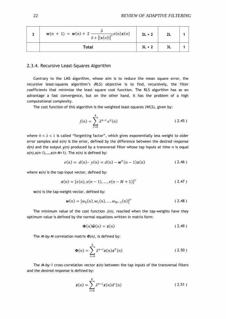
where d(n) is the desired response; wo is the vector which represents the system, having
dimension (7,1) in this example; x(n) is the input vector, composed by the input x(n) and
having dimension identical to wo; e(n) is the error and y(n) is the filter‟s output.
The figure 3.6 shows the result of applying a RLS algorithm to the system identification
problem. The RLS was initialized with ( ) . The result of simulations pointed
as the best value for this constant which is multiplied to the Identity matrix I. The forgetting
factor λ was set to be 0.9.
L = 7, SNR = 40dB, λ = 0.9
Figure 3.6 - Desired signal, filter output and the error of the RLS algorithm for the given system identification‟s problem
Analysing the figure 3.6, by looking to the red line, which represents the error, it can be
observed that the RLS algorithm reaches a tracking behaviour near to its optimum, after
approximately 50 iterations of the program, within the error tending to zero.
The figure 3.7 depicts the behaviour of the RLS‟s cost function, the weighted least-
squares. After 50 or 60 iterations, the least-squares become close to the value of the variance
of the noise, which is 0.01 or – 40dB.

32 COMPUTER EXPERIMENTS WITH ADAPTIVE FILTERS
L = 7, SNR = 40dB, λ = 0.9
Figure 3.7 – Weighted least-squares of the RLS algorithm
3.1.5. Comparisons of Results
In real-time applications, it is very important to analyse all the important details before
we choose an adaptive algorithm. A small difference could result in elevated cost of
implementation, or in a weak system, which is not stable in all variable changes, or even the
solution is impossible to be implemented. The choice between using one algorithm instead of
another, to the system identification problem, depends mainly on the following factors:
Rate of Convergence: number of iterations required by the algorithm, to converge to
a value close to the optimum Wiener solution in the mean-square sense. If the
algorithm has a fast rate of convergence, it means that the algorithm adapts rapidly
to a stationary unknown environment.
Computational cost: when we talk about computational cost, it includes
implementation cost, amount necessary to implement the algorithm in a computer
and the number of arithmetic operations. The order of the operations is also
important as well as the memory allocation, which is the space necessary to store the
data and the program.
Tracking: capacity of the algorithm to track statistical variations in a stationary
unknown environment.

33
In this particular application, those three factors have has been analysed. The tracking
factor has been analysed in two stages, one after a few hundred of iterations and the other
after a few thousand iterations.
The tables 2.2, 2.4 and 2.6, presented in the subsections 2.3.1, 2.3.2 and 2.3.3
respectively, show the computational cost of each algorithm. By analysing those tables, we
can detect that the RLS algorithm has a maximum complexity of L2 against L to the LMS and
NLMS. It means that the RLS algorithm requires a higher processing power than the other two.
It implies higher cost of hardware.
The figure 3.8 shows a comparison between the rates of convergence of the three
proposed algorithms. Investigating the results shown in figure 3.8, it can be detect that the
rate of convergence of the RLS algorithm is faster than the other two. Indeed, it can be twice
faster than the NLMS and three times faster than the LMS algorithm.
L = 7, SNR = 40dB, µ = 0.02(LMS), δ = 0.9, µ = 0.25(NLMS), λ = 0.9
Figure 3.8 - Comparison between the algorithms cost function
The next analysis is about the value of the prediction error e(n). The figure 3.9 depicts a
comparison between the error of the three algorithms during the consecutives iterations of
the algorithms. By examining the result, it can be noticed that the RLS algorithm has an error
close enough to its optimum Wiener solution in a small number of iterations, about 50
iterations. The RLS presents another good characteristic, which is why it converges to the
optimum value of the error prediction, stabilizing nearby this value without big variations
since the 50th iteration and during all the period shown in the illustration. The LMS error

34 COMPUTER EXPERIMENTS WITH ADAPTIVE FILTERS
prediction starts to converge about 80 iterations, but the disturbance is too big until about
110 iterations, when it starts to show some stability, but still having small disturbances during
all the period shown. The NLMS algorithm shows a better response than the LMS, but still
slower than the RLS algorithm.
L = 7, SNR = 40dB, µ = 0.02(LMS), δ = 0.9, µ = 0.25(NLMS), λ = 0.9
Figure 3.9 - Comparison between the error signals of the algorithms until a few hundred iterations
Exploring Figure 3.9, it can be said that if you want a faster convergence when you are
identifying a system, the RLS is the best possible solution, but it is not the only reason why it
should be studied. Figure 3.10 shows a comparison between the errors from the three
algorithms, after more than a thousand iterations. It can be noticed that the error variations
start to be bigger for the RLS than for the LMS algorithm. It is the opposite of what was
happening after a few hundred iterations. It is reasonable because the LMS based algorithms
are model independent, when the RLS algorithm is model dependent. It means that unless the
standard RLS algorithm matches with the underlying model of the environment in which it
operates, we would expect a degradation of the performance of the RLS algorithm, due to
the mismatch [18]. This problem explains why the LMS based algorithms exhibits a better
tracking behaviour.

35
L = 7, SNR = 40dB, µ = 0.02(LMS), δ = 0.9, µ = 0.25(NLMS), λ = 0.9
Figure 3.10 - Comparison between the error signals of the algorithms after a thousand iterations
3.2. Linear Prediction
In the linear prediction problem [40-45], the aim is to predict the value of an unknown
signal without having any prior knowledge. The linear prediction can be used to predict
measurement error of noise sensors, trajectory of objects in video image and many other
applications. This section presents a solution for a given problem of prediction, using the
adaptive filter algorithms covered in this study.
3.2.1. The problem
Figure 3.11 depicts an adaptive filter for the prediction problem. As it can be observed,
the scheme consists of a random signal, represented by a sinusoid. The filter‟s desired
response x(n), a delayed version of the random signal u(n) is the adaptive filter‟s input, the
filter generates an output y(n) which is one of the outputs, the error e(n) is a result of the
difference between the desired response d(n) added to the white Gaussian noise n(n) with
zero mean and variance 0.01 and the filter output y(n) (e(n)=d(n)+n(n)–y(n)). The error e(n) is
the second system output.

36 COMPUTER EXPERIMENTS WITH ADAPTIVE FILTERS
Figure 3.11 - Adaptive filter for linear prediction
3.2.2. The LMS Solution
In order to apply the LMS to the prediction problem, some alterations in the summary
presented in Section 2.3 will be introduced. After doing the necessary changes, we get the
following equations:
( ) ( ) ( 3.6 )
( ) ( ) ( ) ( 3.7 )
( ) ( ) ( ) ( ) ( 3.8 )
( ) ( ) ( ) ( ) ( 3.9 )
where x(n) is the random input signal; u(n) is the delayed version of x(n); d(n) is the desired
adaptive filter‟s response; w(n) is the tap-weight vector with variable length (chosen to be 7
in this program); u’(n) is the vector composed by the delayed version u(n) of the input signal;
y(n) is the filter‟s output; the prediction error e(n) is given by the desired response d(n) plus
the noise n(n) minus the filter output y(n) and µ is the step-size parameter.
The figure 3.12 illustrate the desired response d(n) (blue line) being tracked for the filter
output y(n) (green line) and the error e(n) (red line), resultant of this comparison. It can be
noticed that the algorithm presents a small error, near to its optimum value, about 2000
iterations after the initialization. The step-size µ was chosen to be equal to 0.01 after tests
analysing the mean-squared error.

37
L = 7, SNR = 40dB, µ = 0.01
Figure 3.12 - Desired signal, filter output and error of the LMS algorithm for the prediction given problem

38 COMPUTER EXPERIMENTS WITH ADAPTIVE FILTERS
L = 7, SNR = 40dB, µ = 0.01
Figure 3.13 - Mean-squared-error of the LMS algorithm
The figure 3.13 depicts the mean-squared error of the algorithm. By studying this figure,
it can be detected that the algorithm converges after about the 2000th iteration, converging
to the variance of the noise n(n) 0.01 or – 40dB.
3.2.3. The NLMS Solution
For applying the NLMS algorithm to the given prediction problem, the equations displayed
in the table 2.3 will be adapted from the summary of the NLMS algorithm. Performing the
necessary modification, we end with the following equations:
( ) ( ) ( 3.10 )
( ) ( ) ( ) ( 3.11 )
( ) ( ) ( ) ( ) ( 3.12 )
|| ( )|| ( 3.13 )
( ) ( ) ( ) ( ) ( )
|| ( )|| ( ) ( ) ( 3.14 )

39
where x(n) is the random input signal; u(n) is the delayed version of x(n); d(n) is the desired
adaptive filter‟s response; w(n) is the tap-weight vector with variable length (chosen to be 7
in this program); u’(n) is the vector composed by the delayed version u(n) of the input signal;
y(n) is the filter‟s output; the prediction error e(n) is given by the desired response d(n) plus
the noise n(n) minus the filter output y(n); µ is the LMS step-size parameter; is the NLMS
step-size parameter and δ is a small positive constant.
The figure 3.14, presented below, illustrate the results obtained after the application of
the NLMS algorithm to the given prediction problem. It can be verified that after about 300
iterations, the algorithm presents a reasonable error, having its value tending to the optimum
solution (in some sense). The step-size and the constant δ was chosen to be equal to 0.1
and 0.3 respectively, after tests analysing the mean-squared error.
L = 7, SNR = 40dB, δ = 0.3, = 0.1
Figure 3.14 - Desired signal, filter output and error of the NLMS algorithm for the system identification given problem
The NLMS cost function, the mean-squared error, is depicted in figure 3.15. The objective
of this cost function is to reduce the error until it tends to the optimum solution. It can be
understood, after the analysis of this figure, that the error starts converging after about 250,
300 iterations, with the MSE reaching a value near to 0.01 or – 40dB, which is the same value
of the noise variance.

40 COMPUTER EXPERIMENTS WITH ADAPTIVE FILTERS
L = 7, SNR = 40dB, δ = 0.3, = 0.1
Figure 3.15 - Mean-squared-error of the NLMS algorithm
3.2.4. The RLS Solution
The computation of the RLS solution for the given prediction problem is done using the
summary present in table 2.5. Some alterations will be needed in order to fit this algorithm
to the given problem. The results of the alterations in the RLS equations are:
( ) ( ) ( 3.15 )
( )
( ) ( )
( ) ( ) ( )
( 3.16 )
( ) ( ) ( ) ( 3.17 )
( ) ( ) ( ) ( ) ( 3.18 )
( ) ( ) ( ) ( ) ( 3.19 )
( )
( ) ( ) ( ) ( ) ( 3.20 )

41
where x(n) is the random input signal; u(n) is the delayed version of x(n); d(n) is the desired
adaptive filter‟s response; k(n) is the gain vector; λ is the forgetting factor; w(n) is the tap-
weight vector with variable length (chosen to be 7 in this program); u’(n) is the vector
composed by the delayed version u(n) of the input signal; y(n) is the filter‟s output; the
prediction error e(n) is given by the desired response d(n) plus the noise n(n) minus the filter
output y(n); A* is the complex conjugate of A and is the cross-correlation matrix. The
forgetting factor was chosen to be equal to 1 after tests analysing the algorithm‟s cost
function.
L = 7, SNR = 40dB, λ = 1
Figure 3.16 - Desired signal, filter output and error of the RLS algorithm for the system identification given problem
The figure 3.16 shows the output filter predicting the desired signal, it can be observed
that after about 30-50 iterations the algorithm starts to present an error near to its optimum
value.
The cost function, least-squares, is depicted in figure 3.17. Analysing that picture, it can
be noticed that after the same number of iterations, about 30-50, the error converges to the
– 40dB, the value of the noise variance 0.01. After the conversion, the algorithm does not
suffer important variations, having good predicting behaviour.

42 COMPUTER EXPERIMENTS WITH ADAPTIVE FILTERS
L = 7, SNR = 40dB, λ = 1
Figure 3.17 – Least-squares of the RLS algorithm
3.2.5. Comparisons of results
The analysis of the three algorithms will be performed according to the factors presented
in Subsection 3.1.5, which are: the rate of convergence, the computational cost and the
tracking characteristics. The computational cost is a fixed factor where the RLS algorithm has
the disadvantage of having a higher computational cost, because of its necessary calculation.
A comparison between the algorithms cost function until 2500 iterations is shown in figure
3.18. It can be easily noticed that the LMS algorithm has a very slow rate of convergence
comparing to the other two algorithms. Indeed, the rate of convergence of the LMS algorithm
was noted to be 8 times smaller than the NLMS algorithm and 40 times smaller than the rate
of convergence of the RLS algorithm. The last one presents the fastest rate of convergence,
which makes it ideal for application were a fast convergence is necessary.

43
L = 7, SNR = 40dB, µ = 0.01(LMS), δ = 0.3, = 0.1(NLMS), λ = 1
Figure 3.18 - Comparison between the algorithms cost function
Figure 3.19 illustrates a comparison of the prediction error between the three algorithms.
The prediction error is inversely proportional to the tracking capability in this case. It
confirms that the RLS algorithm has the best tracking characteristic, maintaining a small error
after its conversion in a period of time smaller than the two others. The figure 3.20 depicts
the same problem, but after 25000 iterations, in order to verify the tracking behaviour of the
algorithms in stationary state. The analysis of this figure implies that there is no big
difference between the tracking behaviour of the algorithms, with only a small advantage of
the LMS algorithm above the other two.
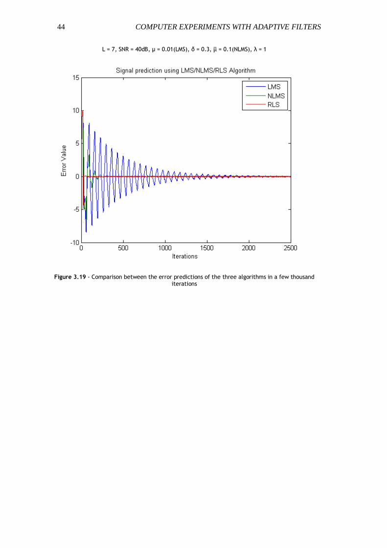
44 COMPUTER EXPERIMENTS WITH ADAPTIVE FILTERS
L = 7, SNR = 40dB, µ = 0.01(LMS), δ = 0.3, = 0.1(NLMS), λ = 1
Figure 3.19 - Comparison between the error predictions of the three algorithms in a few thousand iterations

45
L = 7, SNR = 40dB, µ = 0.01(LMS), δ = 0.3, = 0.1(NLMS), λ = 1
Figure 3.20 - Comparison between the error predictions of the three algorithms after a few hundred thousand iterations
Analysing the results presented in this section it can be assumed that the RLS algorithm,
even having a higher computational cost, presents a faster response for prediction
applications in real time, maintaining a good tracking ability.
The next chapter presents computer experiments for the ANC problem. It presents
solutions using the three (LMS, NLMS, RLS) discussed algorithms and their results. There will
be also presented a comparison between the results and the relevant characteristics of each
algorithm solution.

46 COMPUTER EXPERIMENTS WITH ADAPTIVE FILTERS

47
4. General ANC computer experiments
After consolidating the understanding of the adaptive filter theory during the last sections
and presenting possible solutions for some applications of the AF, now it is the time to work
on a solution for the chosen application, which is the adaptive noise cancellation problem [6-
11, 26-39].
In Section 4.1, a generic problem of noise interference will be explained. Moreover,
solutions for the three adaptive algorithms discussed previously in this work will be
presented.
After the theory presented about the ANC and the simulations for a generic noise
interference problem, it will be given, in the chapter 5, a solution in Simulink environment
for a more specific problem, which will be the Active Noise Canceller for Speech
interference.
Here it is presented a generic problem of noise interference and solutions provided by
using the three algorithms used in this work: LMS, NLMS and RLS. Moreover, a comparison
between them is presented, in order to give the reader a sufficient knowledge to choose the
best solution between them, depending on the application.
4.1. The Problem
For the purpose of testing the theory of active noise cancellers presented along this
thesis, a generic problem and a viable solution are being discussed. Firstly it is necessary to
understand the difference between the interference cancelling and the three other classes.
The figure 4.1 helps to understand the ANC‟s logic. In the other applications presented in
this work, the algorithm always had access to the desired response. The desired response was
later on corrupted for a noise and the filter needed to identify and imitate the desired
response in the best possible fit (in some sense).
For the ANC case, this desired response comes already corrupted for a noise. It makes the
problem impossible to be solved using the logic shown until now.

48 GENERAL ANC COMPUTER EXPERIMENTS
Figure 4.1 – The active noise canceller problem
Analysing the figure 4.1, it can be seen that the noise n2(n) which corrupts the desired signal s(n) is represented by the same initial characters as the input signal n1(n) . This noise is conveniently represented as shown, to make easier to understand that the noise n1(n) and n2(n) have some similarities. Indeed, the noise n1(n) is the noise source and the noise n2(n) is a secondary noise which is correlated with n1(n). Both of noises are also uncorrelated with the signal s(n), which implies in the following conditions:
( ) ( ) ( ) ( 4.1 )
, ( ) ( )- ( 4.2 )
, ( ) ( )- ( 4.3 )
, ( ) ( )- ( ) ( 4.4 )
where d(n) is the desired signal, E[ * ] is the expectation and p(n) is an unknown correlation
between n1(n) and n2(n).
Those necessary conditions can be obtained, for example, if it is installed a sensor
sensor1 in a place where only the noise source n1(n) is detected by the sensor. The sensor
sensor2 will detect the desired signal d(n), and the noise n2(n) could be correlated with n1(n)
because of the delay between them, for example, or by applying a filter.
The error signal e(n), which is also the system output should contain the original
signal s(n) in an optimum sense.
The aim of this algorithm is to make the output y(n), which is equal to the filter‟s
tap-weight transposed ( ) times x’(n) (vector formed by the reference noise
signal n1(n) having the same size as w(n)), or ( ) ( ) ( ), be equal to the
noise n2(n) ( ( ) ( )). Having this equivalence, it is easy to deduce that the error
is equal to the desired signal s(n) ( ( ) ( ) ( ) ( ) ( ) ( ) ( )).
To guarantee that n1(n) and n2(n) are correlated, it was created a noise v(n)
uncorrelated with the desired signal having variance 0.8. This signal was filtered in
order to create the both n1(n) and n2(n) noise signals.

49
4.2. The LMS solution
Here is presented a LMS solution for the presented noise cancellation [28-29, 31-33, 35-
39] problem. Keeping in mind the figure 4.1, the summary presented in table 2.1 for the LMS
and doing the necessary alterations to reach the interference cancelling problem, we found
that:
( ) ( ) ( ) ( 4.5 )
( ) ( ) ( 4.6 )
( ) ( ) ( ) ( 4.7 )
( ) ( ) ( ) ( 4.8 )
( ) ( ) ( ) ( ) ( 4.9 )
where x(n) is a signal composed by the original signal s(n) added to the noise signal n1(n); d(n)
is the desired system output; y(n) is the ANC‟s output; w(n)is the tap-weight vector; x’(n) is
the vector formed by the reference noise signal n1(n) having the same size like w(n); e(n) is
the error signal and µ is the step-size parameter.
The figure 4.2 and 4.3 depicts the results obtained by applying the LMS algorithm for the
given problem, containing the input signal s(n), the desired signal x(n)=s(n) + n2(n) and the
error signal, which should be equal to the input signal s(n). The step-size parameter was
chosen to be equal to 0.0002 and the adaptive filter has length 5. It can be seen in blue, the
signal s(n), the input signal. In green color it is presented the input signal after the noise
corruption s(n) + n2(n), and in red, the error signal e(n).

50 GENERAL ANC COMPUTER EXPERIMENTS
L = 5, µ = 0.0002
Figure 4.2 - Results of application of the LMS algorithm to the given problem
Analysing those figures, specially Figure 4.3 (zoom of part of the figure 4.2), it can be
seen that the LMS algorithm has not a very good performance, having the error signal e(n)
tending to the original signal s(n), free of the noise interference n1(n).

51
L = 5, µ = 0.0002
Figure 4.3 - Zoom of results shown in figure 4.2

52 GENERAL ANC COMPUTER EXPERIMENTS
L = 5, µ = 0.0002
Figure 4.4 - Mean-squared error of the ANC using the LMS algorithm
Figure 4.4 shows the mean-squared error for the LMS algorithm applied to the ANC
problem. This error is not the error signal e(n) but the difference between this signal and the
input signal s(n). As it can be detected, even until 30000 iterations, the algorithm does not
present a convergence. In practice, it means that the algorithm should have a good quantity
of iterations (a few seconds) until the error reaches a value near to its optimum in the mean-
square sense.
4.3. The NLMS solution
The goal now is to apply the NLMS algorithm to the presented noise cancellation problem
[33-34, 36]. In order to do that, some manipulations will be made in the equations presented
in the NLMS summary in table 2.3 to solve the interference cancelling problem. Doing the
necessary modification, we will end with the following equations:
( ) ( ) ( ) ( 4.10 )
( ) ( ) ( 4.11 )

53
( ) ( ) ( ) ( 4.12 )
( ) ( ) ( ) ( 4.13 )
( ) ( ) ( ) ( ) ( 4.14 )
|| ( )|| ( 4.15 )
where x(n) is a signal composed by the original signal s(n) added to the noise signal n2(n); d(n)
is the desired system output; y(n) is the ANC‟s output; w(n)is the tap-weight vector; x’(n) is
the vector formed by the reference noise signal n1(n) having the same size like w(n); e(n) is
the error signal and µ is the LMS step-size parameter which is replaced by a new value,
containing the NLMS step-size parameter , a small positive constant δ and having || * ||
representing the Euclidean norm of *.
The application of the algorithm described above, having the small positive constant δ
equal to 3.2 and the NLMS step-size parameter equal to 0.005, has resulted in the
following:
L = 5, δ = 3.2, µ = 0.005
Figure 4.5 - Results of application of the NLMS algorithm to the given problem

54 GENERAL ANC COMPUTER EXPERIMENTS
L = 5, δ = 3.2, µ = 0.005
Figure 4.6 - Zoom of results shown in figure 4.5
Figures 4.5 and 4.6 depict the results of the application of the ANC using the NLMS
algorithm. The input signal s(n), represented by the blue color is corrupted by the noise signal
n1(n) resulting in the corrupted signal x(n)=s(n)+n2(n), represented by the green color. The
error signal e(n), which is supposed to imitate the input signal s(n) is represented by the red
color.
By analysing the figures above, especially the figure 4.6, it can be noticed that the
algorithm has a good response, cancelling the additional white noise which was corrupting the
original signal.
The figure 4.7, depicts the MSE of the difference between the error signal e(n) and the
input signal s(n). It can be observed that the algorithm presents a conversion after about
10000 iterations. After this time, the algorithm presents some variance but the conversion is
not compromised.

55
L = 5, δ = 3.2, µ = 0.005
Figure 4.7 - Mean-squared error of the ANC using the NLMS algorithm
4.4. The RLS solution
In this section, it will be presented an ANC for noise cancelling [27, 30, 34]. Observing the
figure 4.1, necessary alterations can be made in the summary for the RLS algorithm presented
in subsection 2.3.4 in order to reach the ANC problem presented in Section 4.1. Doing the
needed alterations, the resultant RLS algorithm for noise cancellation can be written as:
( ) ( ) ( ) ( 4.16 )
( ) ( ) ( 4.17 )
( )
( ) ( )
( ) ( ) ( )
( 4.18 )
( ) ( ) ( ) ( 4.19 )
( ) ( ) ( ) ( 4.20 )
( ) ( ) ( ) ( ) ( 4.21 )

56 GENERAL ANC COMPUTER EXPERIMENTS
( )
( ) ( ) ( ) ( ) ( 4.22 )
where x(n) is a signal composed by the original signal s(n) added to the noise signal n2(n); d(n)
is the desired system output; k(n) is the gain vector; λ is the forgetting factor; w(n)is the tap-
weight vector; x’(n) is the vector formed by the reference noise signal n1(n) having the same
size like w(n); y(n) is the ANC‟s output; e(n) is the error signal; A* is the complex conjugate
of A and is the cross-correlation matrix.
The algorithm is initialized with λ equal to 1 and the cross-correlation matrix ( )
, having δ equal to 20 and I been an identity matrix with the same size as .
Figures 4.8 and 4.9 depict the results of the application of the RLS algorithm explained
before in the noise cancelling problem. It can be noted that the algorithm has a good
performance while working as an ANC. The blue line represents the original input signal s(n),
the green line represents the same signal after the noise corruption x(n)=s(n)+n2(n) and the
red line represents the error signal, which should be, and indeed it is, close to the original
input signal s(n).
L = 5, λ = 1
Figure 4.8 - Results of application of the RLS algorithm to the given problem
57
L = 5, λ = 1
Figure 4.9 - Zoom of results shown in figure 4.8
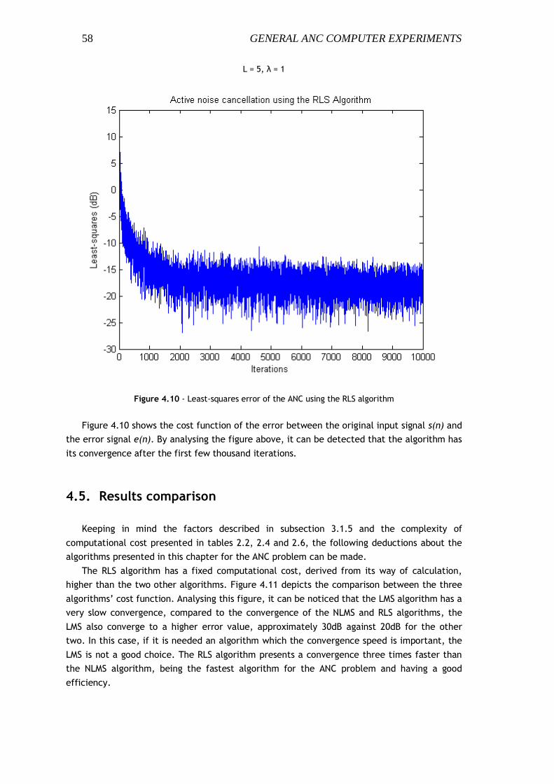
58 GENERAL ANC COMPUTER EXPERIMENTS
L = 5, λ = 1
Figure 4.10 - Least-squares error of the ANC using the RLS algorithm
Figure 4.10 shows the cost function of the error between the original input signal s(n) and
the error signal e(n). By analysing the figure above, it can be detected that the algorithm has
its convergence after the first few thousand iterations.
4.5. Results comparison
Keeping in mind the factors described in subsection 3.1.5 and the complexity of
computational cost presented in tables 2.2, 2.4 and 2.6, the following deductions about the
algorithms presented in this chapter for the ANC problem can be made.
The RLS algorithm has a fixed computational cost, derived from its way of calculation,
higher than the two other algorithms. Figure 4.11 depicts the comparison between the three
algorithms‟ cost function. Analysing this figure, it can be noticed that the LMS algorithm has a
very slow convergence, compared to the convergence of the NLMS and RLS algorithms, the
LMS also converge to a higher error value, approximately 30dB against 20dB for the other
two. In this case, if it is needed an algorithm which the convergence speed is important, the
LMS is not a good choice. The RLS algorithm presents a convergence three times faster than
the NLMS algorithm, being the fastest algorithm for the ANC problem and having a good
efficiency.

59
L = 5, µ = 0.0002(LMS), δ = 0.9, µ = 0.0083(NLMS), λ = 1
Figure 4.11 - Comparison between the algorithms cost function
The next chapter presents computer simulations of the ANC problem using Matlab
Simulink platform. Those simulations intend to show the algorithm working in a most practical
application. The components used in those simulations can be replaced by a physical
component without big changes in the results.

60 GENERAL ANC COMPUTER EXPERIMENTS

61
5. Computer simulation with ANC
This section presents examples of the active noise canceller being used in different
situations. The first subsection presents a solution using the LMS algorithm, in the second
section the RLS algorithm will be used for the same situations.
5.1. The program
In order to present the performance of the program in both ideally theoretical and a
practical environment, the program will be used for cancel a white Gaussian noise and a
colored noise. The figure 4.12 illustrates the proposed problem for the ANC using both
algorithms. Moreover, this image is detailed using the legend presented below.
Figure 5.1 - Proposed problem for the active noise canceller
1 – Input signal s(n), represented by an .avi file containing a speech within sampling
frequency 22050 Hz. This signal is the 1st input of the scope.
2 – Source noise signal n1(n). White Gaussian with zero mean and variance equals to 0.1
(20dB) used as filter input.
3 – Direct-form FIR Lowpass filter from the 10th order. Used to create a second noise
n2(n), correlated with the source noise n1(n).

62 COMPUTER SIMULATION WITH ANC
4 – Sum. Used to add the Input signal s(n) to the noise signal n2(n) generation the desired
signal d(n)=s(n)+n2(n). The desired signal d(n) is the 2nd input of the scope.
5 – Constant. It stores the value of the constant µ for the LMS algorithm or constant λ for
the RLS algorithm.
6 – On-off switch. It turns on or of the adapt port of the filter. The adapt port is
responsible for turn on/off the tap-weight filter w(n) adaptation.
7 – Adaptive filter. LMS or RLS adaptive filter blocks containing all necessary inputs and
outputs.
8 – Squared error. The sum is responsible for calculate de error between the input signal
s(n) and the error signal e(n). This resultant signal is then squared using the product block.
This signal is the 4th input of the scope.
9 – Terminator. It is used to terminate unconnected output port.
10 – Scope. It is necessary to present all the inputs in real-time in a graphic window.
11 – To audio device. It transfer the error signal e(n), output of the adaptive filter, to the
speakers device.
For the case of the colored noise, the Noise block is replaced by the input audio device
and the signal n1(n) is going to be a random signal received throughout the microphone.
For computational reasons, after tests, the length of the LMS algorithms was chosen to be
32 and the length of the RLS algorithms is equal to 12.
5.2. Simulation using the LMS algorithm
This section presents the simulations and results of the LMS algorithm for the case of the
white Gaussian noise and the colored noise corruption the input signal.
5.2.1. Input signal corrupted by a white Gaussian noise
The active noise canceller program, using the LMS solution for a signal corrupted by a
white Gaussian noise is illustrated in figure 4.13. For this simulation, the filter length was
chosen to be equal to 32.

63
Figure 5.2 - LMS active noise canceller using a white Gaussian noise
The filter has length 32 and the noise has variance 0.1. The step-size parameter µ was
chosen to be 0.0008. This value was selected after tests and analysing the similarity between
the input signal and the error signal.
The figure 5.3 presents the signals: Original signal s(n) – input signal without noise; Signal
+ Noise – input signal s(n) added to the noise n2(n), used as the desired response d(n); Error
signal e(n) – Signal resultant of the subtraction of the desired response d(n) by the filter
output y(n); Squared error – difference between the original input signal s(n) and the filter‟s
error signal e(n). Studying this figure, it can be observed that the algorithm takes about 1
second to present an acceptable conversion characteristic, having the squared error tending
to zero.

64 COMPUTER SIMULATION WITH ANC
Figure 5.3 - Relevant signals and algorithm‟s convergence
Figure 5.4 illustrates the behaviour of the algorithm after 10 seconds of work. After this
time, the algorithm presents an error near to its optimum value, with average error from the
order of 2x10⁻⁴, without having big variations.

65
Figure 5.4 - Relevant signal and squared error after 10 seconds
5.2.2. Input signal corrupted by a colored noise
The filter length was chosen to be 32. The input signal is now corrupted by a colored
noise. This colored noise is random and detected by the microphone input. The figure 5.5
illustrates the LMS program using a colored noise to corrupt the input signal.
Figure 5.5 - LMS active noise canceller using colored noise

66 COMPUTER SIMULATION WITH ANC
Figure 5.6 - Relevant signals and algorithm convergence
In the figure 5.6 are presented the following signals: Original signal s(n) – input signal
without noise; Signal + Noise – input signal s(n) added to the noise n2(n), used as the desired
response d(n); Error signal e(n) – Signal resultant of the subtraction of the desired response
d(n) by the filter output y(n); Squared error – difference between the original input signal s(n)
and the filter‟s error signal e(n). Analysing this figure, it can be noticed that the algorithm
takes about 0.3 second to present an acceptable conversion characteristic, having the
squared error tending to zero. In the case of the colored noise, the convergence time is not a
fix value and it will vary depending on the power of the interference at that time.
The figure 5.7 depicts the algorithm behaviour after its convergence. The analysis of the
figure 5.7 can deduce that the algorithm has a bigger squared error (having values from the
order of 0.02 to the colored noise against 2x10⁻⁴ for the white noise) when dealing with a
colored noise than when it was dealing with a white Gaussian noise. Indeed, the error is even
possible to be heard because of its high value. It happens because every time that the noise
present a suddenly variation, the algorithm needs to work as in the beginning to converge
again, and for the case of the LMS algorithm it usually takes some time.

67
Figure 5.7 - Relevant signal and squared error after the algorithm has converged
5.3. Simulation using the RLS algorithm
This section presents the application of a RLS program to the ANC problem, having both
white Gaussian noise and colored noise as interference to the original signal. For this
simulation, the filter length was chosen to be equal to 12.
5.3.1. Input signal corrupted by a white Gaussian noise
The figure 5.8 contains the ANC program built to work with a signal being corrupted by a
white Gaussian noise. The filter has length 12 and the noise has variance 0.1. The forgetting-
factor λ was chosen to be equal to 1, after hearing tests.

68 COMPUTER SIMULATION WITH ANC
Figure 5.8 - RLS active noise canceller using a white Gaussian noise
Figure 5.9 depicts the following relevant signals: Original signal s(n) – input signal without
noise; Signal + Noise – input signal s(n) added to the noise n2(n), used as the desired response
d(n); Error signal e(n) – Signal resultant of the subtraction of the desired response d(n) by the
filter output y(n); Squared error – difference between the original input signal s(n) and the
filter‟s error signal e(n). This figure is a good method to show the algorithm convergence. It
can be seen that between the seconds 3.42 and 3.43 the algorithm is turned on and it
converges. The convergence takes a little time, less than 0.01 seconds.
Figure 5.9 - Relevant signals and algorithm‟s convergence

69
Figure 5.10 presents the algorithm behaviour of the algorithm a few seconds after its
convergence. It can be noticed that the algorithm presents a very good performance, with the
squared error having values near to 1x10⁵ and small variation in the squared error.
Figure 5.10 - Relevant signal and squared error a few seconds after the convergence
5.3.2. Input signal corrupted by colored noise
The ANC using the RLS algorithm for cancelling a colored noise is illustrated in figure 5.11.
The filter length is equal to 12. The forgetting factor λ had the best response in the realized
tests.

70 COMPUTER SIMULATION WITH ANC
Figure 5.11 - RLS active noise canceller using colored noise
Figure 5.12 depicts the following signals: Original signal s(n) – input signal without noise;
Signal + Noise – input signal s(n) added to the noise n2(n), used as the desired response d(n);
Error signal e(n) – Signal resultant of the subtraction of the desired response d(n) by the filter
output y(n); Squared error – difference between the original input signal s(n) and the filter‟s
error signal e(n). As it can be seen in this figure, the rate of convergence is so high, that we
cannot see de error convergence curve. This algorithm has indeed a rate of convergence of
the order of 1000 iterations. The sampling frequency of the audio file is 22050Hz witch gives
us a convergence in about 0.22 seconds.
Figure 5.12 - Relevant signals and algorithm convergence

71
Figure 5.13 presents the signal values after the algorithm‟s convergence. It can be seen
that the algorithm maintains its efficiency even with the noise sudden variations.
Figure 5.13 - Relevant signal and squared error after the algorithm has converged

72 COMPUTER SIMULATION WITH ANC

73
6. Conclusion and Future work
The study presented in this work describes the adaptive filter theory and presents
solutions for the four basic classes of applications. It goes deeper in the active noise
cancellation problem, presenting solutions with the three most popular algorithms for a
general ANC problem. Furthermore, it focuses on a specific situation, which is the
interference cancelling in speech signal. It explores a typical noise cancelling problem in
speech signal situation in Simulink platform, having both white Gaussian and colored noise as
interference source. The simulation is being performed for both a LMS algorithm and a RLS
algorithm.
The study proves that the RLS algorithm is more robust than the LMS algorithm,
having a smaller error and a faster convergence for the case of the white Gaussian noise
interference. For the colored noise interference problem, the RLS has presented a part from
the previous advantages, a powerful stability, being capable of keeping its cancellation
quality even with non-white variation in the noise source. It is the opposite to the LMS
algorithm, which has proved its inefficiency in such environment, having big variations in the
noise cancellation error when the colored noise presented a strong signal. Those error
variations are big enough to be listened in the error output signal.
The RLS algorithm has a bigger complexity and computational cost, but depending on the
quality required for the ANC device, it is the best solution to be adopted.
The proposed continuation of this work is to build a prototype of the ANC using the RLS
algorithm. The program would be converted to C programming language or any other
programming language compatible with the controller. The prototype will be composed of a
first microphone (microphone 1) positioned in a place that captures only the noise signal; a
second microphone (microphone 2) which captures the corrupted signal and a speaker to
propagate an inverse noise signal in order to cancel the noise interference. The prototype and
expected theoretical result are presented in the figures 6.1 and 6.2, respectively.

74 CONCLUSION AND FUTURE WORK
Figure 6.1 - ANC prototype scheme
Figure 6.2 - Theoretical result of the noise cancellation

75
References
[1] Haykin, S., “Adaptive filter theory”, 3rd Edition, Prentice Hall, 1996
[2] B. Farhang-Boroujeny, “Adaptive Filters: Theory and Applications”, Wiley, 1998
[3] Gale, Z., “GMC Terrain Crossover uses Noise Cancelling Tech to Quiet Cabin, Help
Efficiency”, Truck Trend Magazine, February 25, 2011
[4] Diniz, P. S. R., “Adaptive Filtering – Algorithams and Practical Implementation”,
Thrird Edition, Kluwer Academic Publishers, 2008
[5] Sayed, A.H., “Fundamentals of Adaptive Filtering”, John Wiley & Sons, New Jersey,
2003
[6] Górriz, J.M.; Ramírez, J.; Cruces-Alvarez, S.; Puntonet, C.G.; Lang, E.W.; Erdogmus,
D., “A Novel LMS Algorithm Applied to Adaptive Noise Cancellation”, IEEE Signal
Processing Letters, VOL. 16, NO. 1, January 2009
[7] Tienan, L.; Limo, W.; Baochang, X.; Aihua, X.; Hang, Z., “Adaptive Noise Canceler
and Its Applications for Systems with Time-variant Correlative Noise”, IEEE
Proceedings of the 4° World Congress on Intelligent Control and Automation, June 10-
14, 2002, Shanghai, P.R.China
[8] Shin, D.C.; Nikias, C.L., “Adaptive noise canceler for narrowband/wideband
interferences using higher-order statistics”, IEEE International conference on
Acoustics, Speech, and Signal Processing, 1993
[9] Widrow, B.; Glover Jr., J.R.; McCool, J.M.; Kaunitz, J.; Williams, C.S.; Hearn, R.H.;
Zeidler, J.R.; Dong Jr., E.; Goodlin, R.C., “Adaptive Noise Cancelling: Principles and
Applications”, Proceedings of the IEEE, Vol. 63, no. 12, December 1975
[10] Pota, H.R.; Kelkar, A.G., “Analysis of Perfect Noise Cancelling Controllers”,
Proceedings of the IEEE, International Conference on Control Applications,
Anchorage, Alaska, USA 9 September 25-27,2000

76 REFERENCES
[11] Gu, Y.H.; Bokhoven, W.M.G.V., “Frequency Bin Nonlinear LMS Adaptive Noise
Canceler and Its Application to CO-channel Speech Noise Reduction”, IEEE Circuits
and Systems International Symposium, 1991
[12] Ifeachor, E.C.; Jervis, B.W., “Digital Signal Processing – A Practical Approach”,
Addison-Wesley, 1993
[13] Guan, X.; Chen, X.; Wu, G., "QX-LMS Adaptive FIR Filters For System Identification,"
2nd International Congress on Image and Signal Processing, 2009. CISP '09, vol., no.,
pp.1-5, 17-19 Oct. 2009
[14] General Motors, 2011. “Popular GMC Terrain aims for greater segment territory in
2011”. 17 May 2012, <http://media.gm.com/media/us/en/gmc/veh
icles/terrain/2011.brand_gmc.html >
[15] Chang, S.L.; Ogunfunmi, T., "LMS/LMF and RLS Volterra system identification based
on nonlinear Wiener model," Proceedings of the IEEE, International Symposium on
Circuits and Systems, 1998. ISCAS '98, vol.5, no., pp.206-209 vol.5, 31 May-3 Jun 1998
[16] Wahab, M.A.; Uzzaman, M.A.; Hai, M.S.; Haque, M.A.; Hasan, M.K.; , "Least-squares
optimal variable step-size LMS for nonblind system identification with noise,"
International Conference on Electrical and Computer Engineering, 2008, ICECE 2008,
vol., no., pp.428-433, 20-22 Dec. 2008
[17] Eweda, E., "Comparison of RLS, LMS, and sign algorithms for tracking randomly time-
varying channels," IEEE Transactions on Signal Processing, vol.42, no.11, pp.2937-
2944, Nov 1994
[18] Haykin, S.; Sayed, A.H.; Zeidler, J.; Yee, P.; Wei, P., "Tracking of linear time-variant
systems," IEEE Conference Record on Military Communications Conference, 1995.
MILCOM '95, , vol.2, no., pp.602-606 vol.2, 7 Nov 1995
[19] Widrow, B.; Lehr, M.; Beaufays, F.; Wan, E.; Bilello, M.; “Adaptive Signal Processing”,
Stanford University Department of Electrical Engineering, 1993
[20] Eleftheriou, E.; Falconer, D., "Tracking properties and steady-state performance of
RLS adaptive filter algorithms," IEEE Transactions on Acoustics, Speech and Signal
Processing, vol.34, no.5, pp. 1097- 1110, Oct 1986
[21] Benveniste, A., "Design of monostep and multistep adaptive algorithms for the
tracking of time varying systems," The 23rd IEEE Conference on Decision and Control,
1984, vol.23, no., pp.353-358, Dec. 1984
[22] Bose, 2012. “QuietComfort® 15 Acoustic Noise Cancelling® headphones”. 22 May
2012, <http://www.bose.co.uk/GB/en/home-and-personal-audio/headphones-and-
headsets/acoustic-noise-cancelling-headphones/quietcomfort-15-headphones/>

77
[23] Wallace, R.B.; Goubran, R.A., "Improved tracking adaptive noise canceler for
nonstationary environments," IEEE Transactions on Signal Processing, vol.40, no.3,
pp.700-703, Mar 1992
[24] Feng, Z.; Shi, X.; Huang, H., "An improved adaptive noise cancelling method,"
Canadian Conference on Electrical and Computer Engineering, 1993, vol., no., pp.47-
50 vol.1, 14-17 Sep 1993
[25] Kolinova, M.; Prochazka, A.; Mudrova, M., "Adaptive FIR filter use for signal noise
cancelling," Proceedings of the IEEE, Signal Processing Society Workshop on Neural
Networks for Signal Processing VIII, 1998, vol., no., pp.496-505, 31 Aug-2 Sep 1998
[26] Tokhi, M.O.; Leitch, R.R., "Design and implementation of self-tuning active noise
control systems," IEEE Proceedings on Control Theory and Applications, vol.138, no.5,
pp.421-430, Sep 1991
[27] Bouchard, M.; Quednau, S., "Multichannel recursive-least-square algorithms and fast-
transversal-filter algorithms for active noise control and sound reproduction systems,"
IEEE Transactions on Speech and Audio Processing, vol.8, no.5, pp.606-618, Sep 2000
[28] Miyagi, S.; Sakai, H., "Performance comparison between the filtered-error LMS and
the filtered-X LMS algorithms [ANC]," The 2001 IEEE International Symposium on
Circuits and Systems, 2001, ISCAS 2001, vol.2, no., pp.661-664 vol. 2, 6-9 May 2001
[29] Kajikawa, Y.; Nomura, Y., "Frequency domain active noise control system using
optimal step-size parameters," IEEE International Conference on Acoustics, Speech,
and Signal Processing, 2001, ICASSP '01, vol.5, no., pp.3217-3220 vol.5, 2001
[30] Gnitecki, J.; Moussavi, Z.; Pasterkamp, H., "Recursive least squares adaptive noise
cancellation filtering for heart sound reduction in lung sounds recordings,"
Proceedings of the 25th Annual International Conference of the IEEE on Engineering in
Medicine and Biology Society, 2003, vol.3, no., pp. 2416- 2419 Vol.3, 17-21 Sept. 2003
[31] Das, D.P.; Panda, G.; Nayak, D.K., "Development of Frequency Domain Block Filtered-
s LMS (FBFSLMS) Algorithm for Active Noise Control System," IEEE International
Conference on Acoustics, Speech and Signal Processing, 2006, ICASSP 2006
Proceedings, vol.5, no., pp.V, 14-19 May 2006
[32] Albu, F.; Bouchard, M.; Zakharov, Y., "Pseudo-Affine Projection Algorithms for
Multichannel Active Noise Control," IEEE Transactions on Audio, Speech, and Language
Processing, vol.15, no.3, pp.1044-1052, March 2007
[33] Park, J.H.; Kim,J.; Lee, J.K.; Kim, S.W.; Lee, C.W., "Performance analysis of adaptive
noise canceller in real-time automobile environments," Thirty-Ninth Southeastern
Symposium on System Theory, 2007. SSST '07, vol., no., pp.169-172, 4-6 March 2007

78 REFERENCES
[34] Milani, A.A.; Panahi, I.M.S.; Briggs, R., "Performance Analysis of Sub-Band nLMS, APA
and RLS in fMRI ANC with a Non-Minimum Phase Secondary Path," IEEE International
Conference on Acoustics, Speech and Signal Processing, 2007, ICASSP 2007, vol.2, no.,
pp.II-353-II-356, 15-20 April 2007
[35] Das, D.P.; Panda, G.; Kuo, S.M., "New block filtered-X LMS algorithms for active noise
control systems," Signal Processing, IET , vol.1, no.2, pp.73-81, June 2007
[36] Ryu, B.S.; Lee, J.K.; Kim, J.; Lee, C.W., "The Performance of an adaptive noise
canceller with DSP processor," 40th Southeastern Symposium on System Theory, 2008,
SSST 2008, vol., no., pp.42-45, 16-18 March 2008
[37] Mahmoodzadeh, A.; Abutalebi, H.R.; Agahi, H., "Speech enhancement using a Kalman-
based normalized LMS algorithm," International Symposium on Telecommunications,
2008, IST 2008, vol., no., pp.555-558, 27-28 Aug. 2008
[38] Jaber, M.A.; Massicotte, D., "A robust Dual Predictive Line Acoustic Noise Cancellers,"
16th International Conference on Digital Signal Processing, 2009, vol., no., pp.1-6, 5-7
July 2009
[39] Bai, L.; Yin, Q., "A modified NLMS algorithm for adaptive noise cancellation," IEEE
International Conference on Acoustics Speech and Signal Processing, 2010, ICASSP,
vol., no., pp.3726-3729, 14-19 March 2010
[40] Manikandan, S.; Ebenezer, D., "A New Prediction Based Adaptive Median Filter for
Restoration of Degraded Audio Signals," International Conference on Signal
Processing, Communications and Networking, 2008, ICSCN '08, vol., no., pp.203-207,
4-6 Jan. 2008
[41] Nair, B.B.; Mohandas, V.P.; Sakthivel, N.R.; Nagendran, S.; Nareash, A.; Nishanth, R.;
Ramkumar, S.; Manoj Kumar, D., "Application of hybrid adaptive filters for stock
market prediction," International Conference on Communication and Computational
Intelligence, 2010, INCOCCI, vol., no., pp.443-447, 27-29 Dec. 2010
[42] Tate, C.N.; Goodyear, C.C., "Note on the convergence of linear predictive filters,
adapted using the LMS algorithm," IEEE Proceedings on Electronic Circuits and
Systems, 1983, vol.130, no.2, pp.61-64, April 1983
[43] Huang, H.; Rahardja, S.; Lin, X.; Yu, R.; Franti, P., "Cascaded RLS-LMS Prediction in
MPEG-4 Lossless Audio Coding," IEEE International Conference on Acoustics, Speech
and Signal Processing, 2006, ICASSP 2006 Proceedings, vol.5, no., pp.V, 14-19 May
2006

79
[44] Huang, D. Y.; Su, X. R., "A performance bound for a cascade LMS predictor," IEEE
International Symposium on Circuits and Systems, 2005, ISCAS 2005, vol., no., pp.
3135- 3138 Vol. 4, 23-26 May 2005
[45] Seo, B.S.; Jang, J.; Lee, S.J.; Lee, C.W., "LMS-type self-adaptive algorithms for
predictive decision feedback equalizer," IEEE Global Telecommunications Conference,
1997, GLOBECOM '97, vol.1, no., pp.67-71 vol.1, 3-8 Nov 1997
[46] Goodwin, G. C.; Payne R. L., "Dynamic System Identification: Experiment Design and
Data Analysis", Academic Press, New York, 1997.
[47] Ljung, L.; Soderstrom, T., "Theory and Practice of Recursive Identification", MIT
Press, Cambridge, Mass, 1983.
[48] Ljung, L., "System Identification: Theory for the User". Prentice Hall, Englewood
Cliffs, N.J., 1987

80 REFERENCES

i
APRENDIX I – System identification problem
LMS algorithm
% System identification - LMS algorithm
% R - number of repetitions
% I - iterations
% sigmax - standard deviation of the input signal x
% Wo - plant/system to be identified
% sigman - standard deviation of the noise n
% mi - step-size parameter
% M - misadjustment
% ind - sample index
% MSE - Mean-squared error
% MSEmin - Minimum Mean-squared error
% D - Auxiliar vector to the desired response
% E - Auxiliar vector to the error
% Y - Auxiliar vector to the filter output
clear all
close all
R = 10;
I = 500;
% parameters
sigmax = 1;
sigman = 0.01;
mi = 0.02;
MSE=zeros(I,1);
MSEmin=zeros(I,1);
Y=zeros(I,1);
D=zeros(I,1);
E=zeros(I,1);
Wo = randn(7,1);
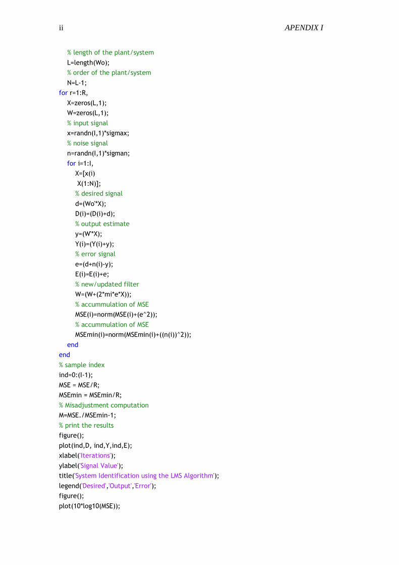
ii APENDIX I
% length of the plant/system
L=length(Wo);
% order of the plant/system
N=L-1;
for r=1:R,
X=zeros(L,1);
W=zeros(L,1);
% input signal
x=randn(I,1)*sigmax;
% noise signal
n=randn(I,1)*sigman;
for i=1:I,
X=[x(i)
X(1:N)];
% desired signal
d=(Wo'*X);
D(i)=(D(i)+d);
% output estimate
y=(W'*X);
Y(i)=(Y(i)+y);
% error signal
e=(d+n(i)-y);
E(i)=E(i)+e;
% new/updated filter
W=(W+(2*mi*e*X));
% accummulation of MSE
MSE(i)=norm(MSE(i)+(e^2));
% accummulation of MSE
MSEmin(i)=norm(MSEmin(i)+((n(i))^2));
end
end
% sample index
ind=0:(I-1);
MSE = MSE/R;
MSEmin = MSEmin/R;
% Misadjustment computation
M=MSE./MSEmin-1;
% print the results
figure();
plot(ind,D, ind,Y,ind,E);
xlabel('Iterations');
ylabel('Signal Value');
title('System Identification using the LMS Algorithm');
legend('Desired','Output','Error');
figure();
plot(10*log10(MSE));

iii
ylabel('Mean-Squared Error (dB)');
xlabel('Iterations');
title('System Identification using the LMS Algorithm');
NLMS algorithm
% System identification - NLMS algorithm
% R - number of repetitions
% I - iterations
% sigmax - standard deviation of the input signal x
% Wo - plant/system to be identified
% sigman - standard deviation of the noise n
% mi - step-size parameter
% M - misadjustment
% ind - sample index
% MSE - Mean-squared error
% MSEmin - Minimum Mean-squared error
% D - Auxiliar vector to the desired response
% E - Auxiliar vector to the error
% Y - Auxiliar vector to the filter output
clear all
close all
% number of iteractions
R = 10;
% number of iteractions
I = 500;
% parameters
sigmax = 1;
sigman = 0.01;
mi = 0.25;
MSE=zeros(I,1);
MSEmin=zeros(I,1);
Y=zeros(I,1);
D=zeros(I,1);
E=zeros(I,1);
Wo = randn(7,1);
% length of the plant/system
L=length(Wo);
% order of the plant/system
N=L-1;
for r=1:R,
X=zeros(L,1);
W=zeros(L,1);
% input signal

iv APENDIX I
x=randn(I,1)*sigmax;
% noise signal
n=randn(I,1)*sigman;
for i=1:I,
X=[x(i)
X(1:N)];
% desired signal
d=(Wo'*X);
D(i)=D(i)+d;
% output estimate
y=(W'*X);
Y(i)=Y(i)+y;
% error signal
e=(d+n(i)-y);
E(i)=E(i)+e;
% new/updated filter
W=(W+(2*(mi/(0.9+(norm(X)^2)))*conj(e)*X));
% accummulation of MSE
MSE(i)=norm(MSE(i)+(e^2));
% accummulation of MSE
MSEmin(i)=norm(MSEmin(i)+((n(i))^2));
end
end
% sample index
ind=0:(I-1);
MSE = MSE/R;
MSEmin = MSEmin/R;
% Misadjustment computation
M=MSE./MSEmin-1;
% print the results
figure();
plot(ind,D, ind,Y,ind,E);
xlabel('Iterations');
ylabel('Signal Value');
title('System Identification using the NLMS Algorithm');
legend('Desired','Output','Error');
figure();
plot(10*log10(MSE));
ylabel('Mean-Squared Error (dB)');
xlabel('Iterations');
title('System Identification using the NLMS Algorithm');
RLS algorithm
%%% System identification - RLS algorithm

v
% R - number of repetitions
% I - iterations
% sigmax - standard deviation of the input signal
% Wo - plant/system to be identified
% sigman - standard deviation of the noise
% ind - sample index
% W - Tap-weight of RLS algorithm
% K - gain
% lambda - Fortgetting factor 1 < lambda < 0
% LS - Weighted least-squares of the rls
% CC - Cross-correlation matrix
% delta - small positive constant
% D - Auxiliar vector to the desired response
% E - Auxiliar vector to the error
% Y - Auxiliar vector to the filter output
clear all
close all
R = 10;
I = 500;
% parameters
sigmax = 1;
sigman = 0.01;
Wo = randn(7,1);
% length of the plant/system
L=length(Wo);
% order of the plant/system
N=L-1;
%%% RLS parameters
lambda = 0.9;
delta = 0.4;
LS=zeros(I,1);
D=zeros(I,1);
Y=zeros(I,1);
E=zeros(I,1);
for r=1:R,
U=zeros(L,1);
% input
u=randn(I,1)*sigmax;
% noise
n=randn(I,1)*0.01;
%%%Initial Conditions RLS
W=zeros(L,1);
CC=((1/delta)*eye(L,L));
for i=1:I,
U=[u(i)

vi APENDIX I
U(1:N)];
% desired signal
d=(Wo'*U);
D(i)=D(i)+d;
%Step 1: Calculation the gain G
k=(((1/lambda)*CC*U)/(1+((1/lambda)*U'*CC*U)));
%Step 2: Filtering
%output estimate for the rls
y=(W'*U);
Y(i)=Y(i)+y;
%Step 3: Error estimation
%error of the rls
e=(d+n(i)-y);
E(i)=E(i)+e;
%Step 4: Tap-weight vector adaptation
W=W+k*conj(e);
%Step 5: Correlation Update
%calculating the CC of the rls algorithm
CC =(((1/(lambda))*CC)-((1/lambda)*k*U'*CC));
% accummulation of LS
LS(i)=(LS(i)+(lambda*e^2));
end
end
% sample index
ind=0:(I-1);
LS = LS/R;
% print the results
figure();
plot(ind,D, ind,Y,ind,E);
xlabel('Iterations');
ylabel('Signal Value');
title('System Identification using the RLS Algorithm');
legend('Desired','Output','Error');
figure();
plot(10*log10(LS));
ylabel('Least-squares (dB)');
xlabel('Iterations');
title('System Identification using the RLS Algorithm');

vii
APRENDIX II – Prediction problem
LMS algorithm
% Prediction - LMS algorithm
% R - number of repetitions
% I - iterations
% sigmax - standard deviation of the input signal
% Wo - plant/system to be identified
% sigman - standard deviation of the noise
% mi - step size
% M - misadjustment
% ind - sample index
% MSE - Mean-squared error
% MSEmin - Minimum Mean-squared error
% D - Auxiliar vector to the desired response
% E - Auxiliar vector to the error
% Y - Auxiliar vector to the filter output
clear all
close all
R = 10;
I = 5000;
% parameters
sigmax = 1;
sigman = 0.01;
mi = 0.01;
MSE=zeros(I,1);
Y=zeros(I,1);
D=zeros(I,1);
E=zeros(I,1);
MSEmin=zeros(I,1);
Wo = randn(7,1);
% length of the plant/system
L=length(Wo);

viii APENDIX II
% order of the plant/system
N=L-1;
for r=1:R,
X=zeros(L,1);
W=zeros(L,1);
% input
n = (1:I)';
x = sin(0.0295*pi*n);
% delayed version of the input
delay=zeros(20,1);
xd=[delay
x(1:(I-20))];
% noise
n=randn(I,1)*sigman;
%awgn(n,);
for i=1:I,
X=[xd(i)
X(1:N)];
% desired signal
d=x(i);
D(i)=(D(i)+d);
% output estimate
y=(W'*X);
Y(i)=(Y(i)+y);
% error signal
e=(d+n(i)-y);
E(i)=E(i)+e;
% new/updated filter
W=(W+(2*mi*e*X));
% accummulation of MSE
MSE(i)=norm(MSE(i)+(e^2));
% accummulation of MSE
MSEmin(i)=norm(MSEmin(i)+((n(i))^2));
end
end
% sample index
ind=0:(I-1);
MSE = MSE/R;
MSEmin = MSEmin/R;
% Misadjustment computation
M=MSE./MSEmin-1;
% print the results
figure();
plot(ind,D, ind,Y,ind,E);
xlabel('Iterations');
ylabel('Signal Value');
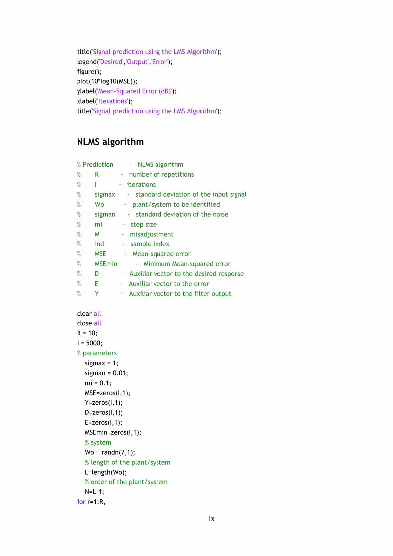
ix
title('Signal prediction using the LMS Algorithm');
legend('Desired','Output','Error');
figure();
plot(10*log10(MSE));
ylabel('Mean-Squared Error (dB)');
xlabel('Iterations');
title('Signal prediction using the LMS Algorithm');
NLMS algorithm
% Prediction - NLMS algorithm
% R - number of repetitions
% I - iterations
% sigmax - standard deviation of the input signal
% Wo - plant/system to be identified
% sigman - standard deviation of the noise
% mi - step size
% M - misadjustment
% ind - sample index
% MSE - Mean-squared error
% MSEmin - Minimum Mean-squared error
% D - Auxiliar vector to the desired response
% E - Auxiliar vector to the error
% Y - Auxiliar vector to the filter output
clear all
close all
R = 10;
I = 5000;
% parameters
sigmax = 1;
sigman = 0.01;
mi = 0.1;
MSE=zeros(I,1);
Y=zeros(I,1);
D=zeros(I,1);
E=zeros(I,1);
MSEmin=zeros(I,1);
% system
Wo = randn(7,1);
% length of the plant/system
L=length(Wo);
% order of the plant/system
N=L-1;
for r=1:R,

x APENDIX II
X=zeros(L,1);
W=zeros(L,1);
% input
n = (1:I)';
x = sin(0.0295*pi*n);
% delayed version of the input
delay=zeros(20,1);
xd=[delay
x(1:(I-20))];
% noise
n=randn(I,1)*sigman;
for i=1:I,
X=[xd(i)
X(1:N)];
% desired signal
d=x(i);
D(i)=(D(i)+d);
% output estimate
S=(Wo*x(i));
y=(W'*X);
Y(i)=(Y(i)+y);
% error signal
e=(d+n(i)-y);
E(i)=E(i)+e;
% new/updated filter
W=(W+(2*(mi/(0.3+(norm(X)^2)))*conj(e)*X));
% accummulation of MSE
MSE(i)=norm(MSE(i)+(e^2));
% accummulation of MSE
MSEmin(i)=norm(MSEmin(i)+((n(i))^2));
end
end
% sample index
ind=0:(I-1);
n = (0:I-1)';
MSE = MSE/R;
MSEmin = MSEmin/R;
M=MSE./MSEmin-1;
% print the results
figure();
plot(n(1:500),[D(1:500), Y(1:500),E(1:500)]);
xlabel('Iterations');
ylabel('Signal Value');
title('Signal prediction using the NLMS Algorithm');
legend('Desired','Output','Error');
figure();

xi
plot(10*log10(MSE));
ylabel('Mean-Squared Error (dB)');
xlabel('Iterations');
title('Signal prediction using the NLMS Algorithm');
RLS algorithm
%%% Prediction - RLS algorithm
% R - number of repetitions
% I - iterations
% sigmax - standard deviation of the input signal
% Wo - plant/system to be identified
% sigman - standard deviation of the noise
% ind - sample index
% W - Tap-weight of RLS algorithm
% K - gain
% lambda - Fortgetting factor 1 < lambda < 0
% LS - Weighted least-squares of the rls
% CC - Cross-correlation matrix
% delta - small positive constant
% D - Auxiliar vector to the desired response
% E - Auxiliar vector to the error
% Y - Auxiliar vector to the filter output
clear all
close all
R = 10;
I = 1000;
% parameters
sigmax = 1;
sigman = 0.01;
mi = 0.02;
lambda = 1;
delta = 0.01;
LS=zeros(I,1);
Y=zeros(I,1);
D=zeros(I,1);
E=zeros(I,1);
MSEmin=zeros(I,1);
Wo = randn(7,1);
% length of the plant/system
L=length(Wo);
% order of the plant/system
N=L-1;
for r=1:R,

xii APENDIX II
X=zeros(L,1);
W=zeros(L,1);
% input
n = (1:I)';
x = sin(0.0295*pi*n);
% delayed version of the input
delay=zeros(20,1);
xd=[delay
x(1:(I-20))];
% noise
n=randn(I,1)*sigman;
%Cross-correlation matrix fi
CC=((1/delta)*eye(L,L));
for i=1:I,
X=[xd(i)
X(1:N)];
% desired signal
d=x(i);
D(i)=(D(i)+d);
%Step 1: Calculation the gain G
k=(((1/lambda)*CC*X)/(1+((1/lambda)*X'*CC*X)));
%Step 2: Filtering
%output estimate for the rls
y=(W'*X);
Y(i)=(Y(i)+y);
%Step 3: Error estimation
%error of the rls
e=((d-n(i))-y);
E(i)=E(i)+e;
%Step 4: Tap-weight vector adaptation
W=W+k*conj(e);
%Step 5: Correlation Update
%calculating the CC of the rls algorithm
CC =(((1/(lambda))*CC)-((1/lambda)*k*X'*CC));
% accummulation of LS
LS(i)=(LS(i)+(lambda*e^2));
end
end
% sample index
ind=0:(I-1);
n = (0:I-1)';
LS = LS/R;
MSEmin = MSEmin/R;
M=LS./MSEmin-1;
% print the results
figure();

xiii
plot(n(1:500),[D(1:500), Y(1:500),E(1:500)]);
xlabel('Iterations');
ylabel('Signal Value');
title('Signal prediction using the RLS Algorithm');
legend('Desired','Output','Error');
figure();
plot(10*log10(LS));
ylabel('Mean-Squared Error (dB)');
xlabel('Iterations');
title('Signal prediction using the RLS Algorithm');

xiv APENDIX II

xv
APRENDIX III – Interference cancellation problem
LMS algorithm
% ANC - LMS algorithm
% R - number of repetitions
% I - iterations
% sigmax - standard deviation of the input signal x
% Wo - plant/system to be identified
% sigman - standard deviation of the noise n
% mi - step-size parameter
% M - misadjustment
% ind - sample index
% MSE - Mean-squared error
% MSEmin - Minimum Mean-squared error
% K - Auxiliar vector to store the error btween the
% orignal signal and the error signal.
% E - Auxiliar vector to the error
clear all;
close all;
R=10;
I=50000;
%Length of the adaptive filter
L=5;
N=L-1;
mi= 0.0002;
MSE=zeros(I,1);
E=zeros(I,1);
K=zeros(I,1);
for r=1:R
%input signal
n = (1:I)';

xvi APENDIX III
s = sin(0.075*pi*n);
%noise source signal
v = 0.8*randn(I,1);
%noise signal 1
ar = [1,1/2];
v1 = filter(1,ar,v);
%input signal + noise 1
x = s + v1;
%noise signal 2
ma = [1, -0.8, 0.4 , -0.2];
v2 = filter(ma,1,v);
%create the signals
%tap-weight and input vector
W=zeros(L,1);
U=zeros(L,1);
for i=1:I
U=[v2(i)
U(1:N)];
% desired signal
d=x(i);
% output estimate
y=(W'*U);
% error signal
e=(d-y);
E(i)=E(i)+e;
K(i)=(s(i)-e);
% new/updated filter
W=(W+(2*mi*e*U));
% accummulation of MSE
MSE(i)=norm(MSE(i)+ (K(i)^2));
% accummulation of MSE
end
end
E=E/R;
MSE=MSE/R;
ind=0:(I-1);
% print the results
figure()
plot(n(9900:10000), [s(9900:10000), x(9900:10000), E(9900:10000)]);
legend('Input signal s(n)', 'signal + noise x(n)','Error = clean signal s(n)');
xlabel('Iterations');
ylabel('Signal Value');
title('Active noise cancellation using the LMS Algorithm');
figure()
plot(10*log10(MSE));
ylabel('Mean-Squared Error (dB)');

xvii
xlabel('Iterations');
title('Active noise cancellation using the LMS Algorithm');
NLMS algorithm
% ANC - NLMS algorithm
% R - number of repetitions
% I - iterations
% sigmax - standard deviation of the input signal x
% Wo - plant/system to be identified
% sigman - standard deviation of the noise n
% mi - step-size parameter
% M - misadjustment
% ind - sample index
% MSE - Mean-squared error
% MSEmin - Minimum Mean-squared error
% K - Auxiliar vector to store the error btween the
% orignal signal and the error signal.
% E - Auxiliar vector to the error
clear all;
close all;
R=10;
I=10000;
%Length of the adaptive filter
L=5;
N=L-1;
mi= 0.005;
MSE=zeros(I,1);
E=zeros(I,1);
K=zeros(I,1);
for r=1:R
%input signal
n = (1:I)';
s = sin(0.075*pi*n);
%noise source signal
v = 0.8*randn(I,1);
%noise signal 1
ar = [1,1/2];
v1 = filter(1,ar,v);
%input signal + noise 1
x = s + v1;
%noise signal 2
ma = [1, -0.8, 0.4 , -0.2];
v2 = filter(ma,1,v);

xviii APENDIX
III
%create the signals
%tap-weight and input vector
W=zeros(L,1);
U=zeros(L,1);
for i=1:I
U=[v2(i)
U(1:N)];
% desired signal
d=x(i);
% output estimate
y=(W'*U);
% error signal
e=(d-y);
E(i)=E(i)+e;
K(i)=(s(i)-e);
% new/updated filter
W=(W+(2*(mi/(3.2+(norm(U)^2)))*conj(e)*U));
% accummulation of MSE
MSE(i)=norm(MSE(i)+(K(i)^2));
% accummulation of MSE
end
end
E=E/R;
MSE=MSE/R;
ind=0:(I-1);
figure()
plot(n(9900:end), [s(9900:end), x(9900:end), E(9900:end)]);
legend('Input signal s(n)', 'signal + noise x(n)','Error = clean signal s(n)');
xlabel('Iterations');
ylabel('Signal Value');
title('Active noise cancellation using the NLMS Algorithm');
% print the results
figure()
plot(10*log10(MSE));
ylabel('Mean-Squared Error (dB)');
xlabel('Iterations');
title('Active noise cancellation using the NLMS Algorithm');
figure()
plot(n(10:10000), [s(10:10000), E(10:10000), K(10:10000)]);
legend('Input signal s(n)', 'signal + noise x(n)','Error = clean signal s(n)');
xlabel('Iterations');
ylabel('Signal Value');
title('Active noise cancellation using the LMS Algorithm');

xix
RLS algorithm
%%% ANC - RLS algorithm
% R - number of repetitions
% I - iterations
% sigmax - standard deviation of the input signal
% Wo - plant/system to be identified
% sigman - standard deviation of the noise
% ind - sample index
% W - Tap-weight of RLS algorithm
% K - gain
% lambda - Fortgetting factor 1 < lambda < 0
% LS - Weighted least-squares of the rls
% CC - Cross-correlation matrix
% delta - small positive constant
% K - Auxiliar vector to store the error btween the
% orignal signal and the error signal.
% E - Auxiliar vector to the error
clear all;
close all;
R=10;
I=10000;
%Length of the adaptive filter
L=5;
N=L-1;
lambda = 1;
delta = 20;
LS=zeros(I,1);
E=zeros(I,1);
K=zeros(I,1);
for r=1:R
%input signal
n = (1:I)';
s = sin(0.075*pi*n);
%noise source signal
v = 0.8*randn(I,1);
%noise signal 1
ar = [1,1/2];
v1 = filter(1,ar,v);
%input signal + noise 1
x = s + v1;
%noise signal 2
ma = [1, -0.8, 0.4 , -0.2];
v2 = filter(ma,1,v);

xx APENDIX III
%create the signals
%tap-weight and input vector
W=zeros(L,1);
U=zeros(L,1);
%Cross-correlation matrix fi
CC=((1/delta)*eye(L,L));
for i=1:I
U=[v2(i)
U(1:N)];
% desired signal
d=x(i);
%Step 1: Calculation the gain G
k=(((1/lambda)*CC*U)/(1+((1/lambda)*U'*CC*U)));
%Step 2: Filtering
%output estimate for the rls
y=(W'*U);
%Step 3: Error estimation
%error of the rls
e=(d-y);
E(i)=E(i)+e;
K(i)=(s(i)-e);
%Step 4: Tap-weight vector adaptation
W=W+k*conj(e);
%Step 5: Correlation Update
%calculating the CC of the rls algorithm
CC =(((1/(lambda))*CC)-((1/lambda)*k*U'*CC));
% accummulation of LS
LS(i)=(LS(i)+(lambda*K(i)^2));
end
end
E=E/R;
LS=LS/R;
ind=0:(I-1);
% print the results
figure()
plot(n(9900:end), [s(9900:end), x(9900:end), E(9900:end)]);
legend('Input signal s(n)', 'signal + noise x(n)','Error = clean signal s(n)');
xlabel('Iterations');
ylabel('Signal Value');
title('Active noise cancellation using the RLS Algorithm');
figure()
plot(10*log10(LS));
ylabel('Least-squares (dB)');
xlabel('Iterations');
title('Active noise cancellation using the RLS Algorithm');