adaptive finite element methods - …chenlong/226/ch4afem.pdf · adaptive finite element methods 3...

ADAPTIVE FINITE ELEMENT METHODS

LONG CHEN

Adaptive methods are now widely used in the scientific computation to achieve betteraccuracy with minimum degree of freedom. In this chapter, we shall briefly survey re-cent progress on the convergence analysis of adaptive finite element methods (AFEMs)for second order elliptic partial differential equations and refer to Nochetto, Siebert andVeeser [14] for a detailed introduction to the theory of adaptive finite element methods.

1. INTRODUCTION TO MESH ADAPTATION

We start with a simple motivation in 1D for the use of adaptive procedures. GivenΩ = (0, 1), a grid TN = xiNi=0 of Ω

0 = x0 < x1 < · · ·xi < · · · < xN = 1

and a continuous function u : Ω → R, we consider the problem of approximating u by apiecewise constant function uN over TN . We measure the error in the maximum norm.

Suppose that u is Lipschitz in [0, 1]. Consider the approximation

uN (x) := u(xi−1), for all xi−1 ≤ x < xi.

If the grid is quasi-uniform in the sense that hi = xi− xi−1 ≤ C/N for i = 1, · · ·N , thenit is easy to show that

(1) ‖u− uN‖∞ ≤ CN−1‖u′‖∞We can achieve the same convergent rate N−1 with less smoothness of the function.

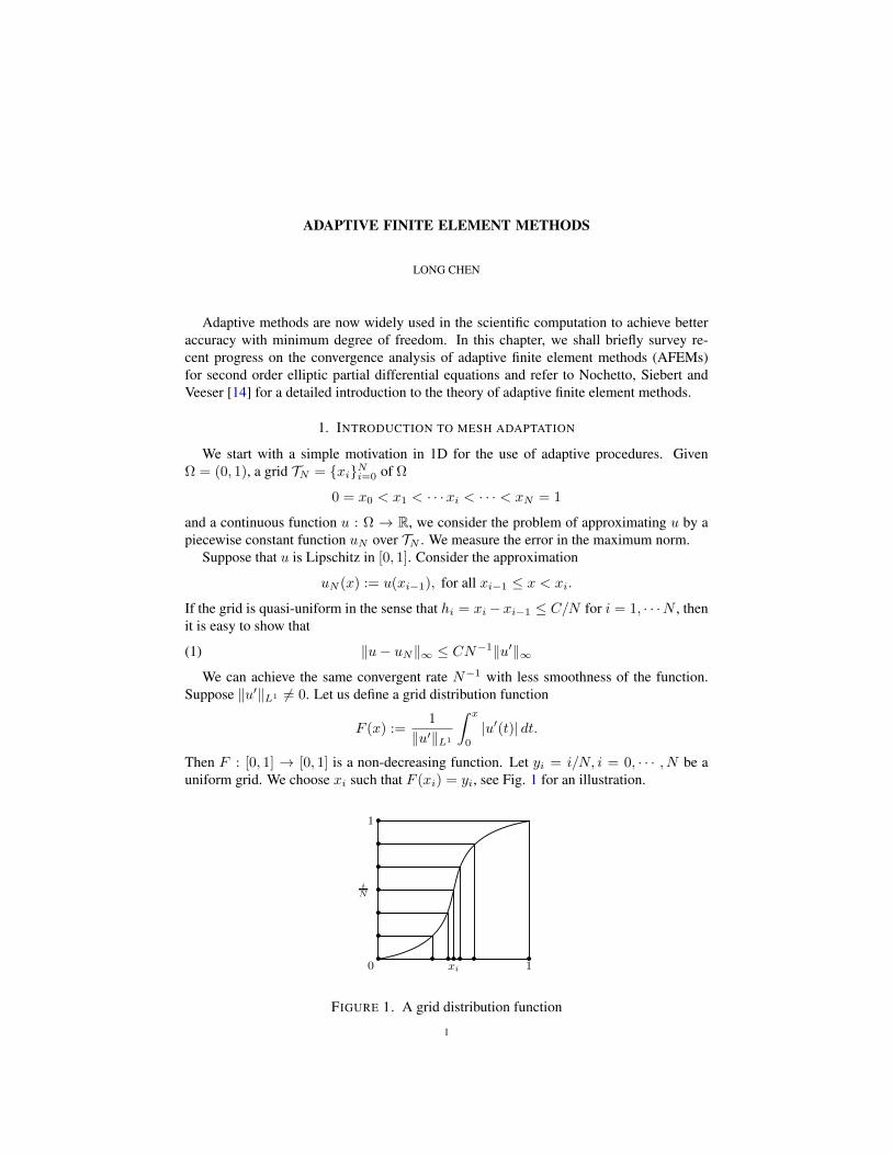
Suppose ‖u′‖L1 6= 0. Let us define a grid distribution function

F (x) :=1

‖u′‖L1

∫ x

0

|u′(t)| dt.

Then F : [0, 1] → [0, 1] is a non-decreasing function. Let yi = i/N, i = 0, · · · , N be auniform grid. We choose xi such that F (xi) = yi, see Fig. 1 for an illustration.

0

1

1

iN

xi

Figure 1: Grid distribution function

1

FIGURE 1. A grid distribution function

1

2 LONG CHEN

Then

(2)∫ xi

xi−1

|u′(t)| dt = F (yi)− F (yi−1) = N−1,

and

|u(x)− u(xi−1)| ≤∫ xi

xi−1

|u′(t)| dt ≤ N−1‖u′‖L1 ,

which leads to the estimate

(3) ‖u− uN‖∞ ≤ CN−1‖u′‖L1 .

We use the following example to illustrate the advantage of (3) over (1). Let us considerthe function u(x) = xr with r ∈ (0, 1). Then u′ /∈ L∞(Ω) but u′ ∈ L1(Ω). Thereforewe cannot obtain optimal convergent rate on quasi-uniform grids while we could on thecorrectly adapted grid. For this simple example, one can easily compute when

xi =

(i

N

)1/r

, for all 0 ≤ i ≤ N,

estimate (3) will hold on the grid TN = xiNi=0 which has higher density of grid pointsnear the singularity of u.

In (2), we choose a grid such that a upper bound of the error is equidistributed. This isinstrumental for adaptive finite element methods on solving PDEs.

A possible MATLAB code is given below.

1 function x = equidistribution(M,x)

2 h = diff(x);

3 F = [0; cumsum(h.*M)];

4 F = F/F(end);

5 y = (0:1/(length(x)-1):1)’;

6 x = interp1(F,x,y);

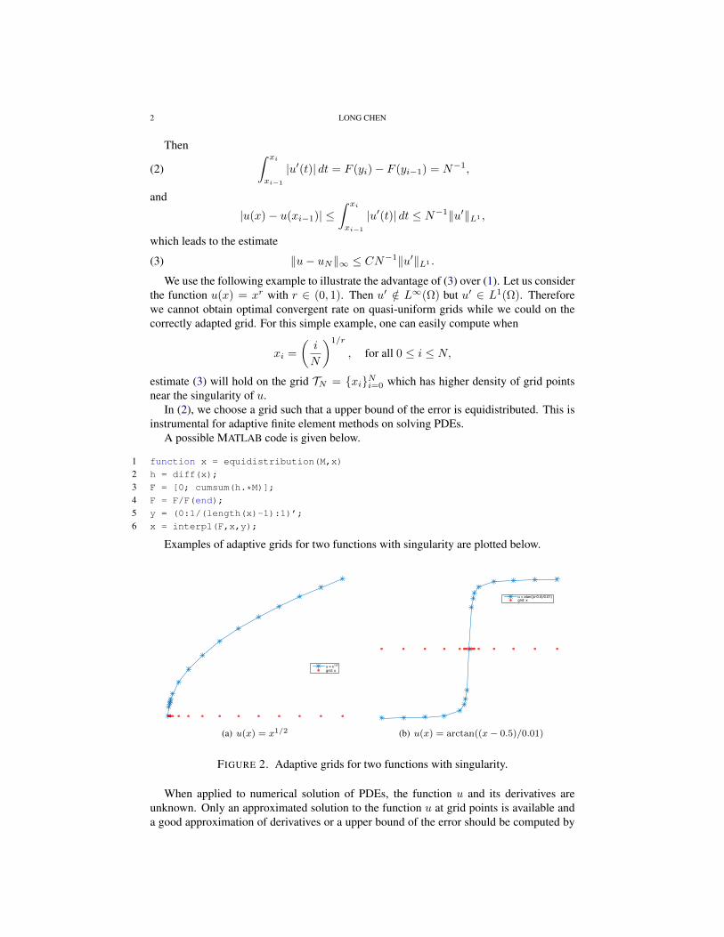
Examples of adaptive grids for two functions with singularity are plotted below.

u = x1/2

grid: x

(a) u(x) = x1/2

u = atan((x-0.5)/0.01)grid: x

(b) u(x) = arctan((x− 0.5)/0.01)

FIGURE 2. Adaptive grids for two functions with singularity.

When applied to numerical solution of PDEs, the function u and its derivatives areunknown. Only an approximated solution to the function u at grid points is available anda good approximation of derivatives or a upper bound of the error should be computed by

ADAPTIVE FINITE ELEMENT METHODS 3

a post-processing procedure. Another difficulty is the mesh requirement in two and higherdimensions. The mesh refinement, coarsening, or movement is much more complicated inhigher dimensions.

Exercise 1.1. We consider the piecewise linear approximation of a second differentiablefunction in this exercise.

(1) When |f | is monotone decreasing, for a positive integer k, prove

1

(k − 1)!

∫ xi+1

xi

|f(x)|(x− xi)k−1 dx ≤ 1

k!

(∫ xi+1

xi

|f(x)|1/k dx

)k.

(2) Let uI be the nodal interpolation of u on a grid, i.e., uI is piecewise linear anduI(xi) = u(xi) for all i. Prove that if |u′′(x)| is monotone decreasing in (xi−1, xi),then for x ∈ (xi−1, xi)

|(u− uI)(x)| ≤(∫ xi

xi−1

|u′′(s)|1/2 ds

)2

.

Hint: Apply the inequality in part (1) to the expansion of u − uI in terms of thebarycentric coordinates; see Exercises in Chapter: Introduction to Finite ElementMethods.

(3) Give the condition on the grid distribution and the function such that the followingestimate holds and prove your result.

‖u− uI‖∞ ≤ C‖u′′‖1/2N−2.

2. SINGULARITY AND EQUDISTRIBUTION

In this section we first present several examples to show that the solution of ellipticequation could have singularity when the domain is concave or the coefficient is discon-tinuous. We then present a theoretical analysis of equidistribution which leads to optimalorder of convergence.

2.1. Lack of Regularity. In FEM, we have obtained a first order convergence of the linearfinite element approximation to the Poisson equation

(4) −∆u = f in Ω, u = 0 on ∂Ω,

provided the solution u ∈ H2(Ω). When the boundary of the domain is smooth or con-vex and Lipschitz continuous, then ∆−1(L2(Ω)) ⊂ H2(Ω). The requirements of Ω isnecessary as shown by the following example.

Consider the domain Ω ⊂ R2 which is defined in a polar coordinate as Ω = (r, θ) :0 < r < 1 and 0 < θ < π

β for 1/2 < β <∞. Obviously if β ≥ 1 then Ω is convex, whileif 1/2 < β < 1 then Ω violates the condition of the regularity theory. Set v = rβ sin(βθ)as the imaginary part of the analytic function zβ , i.e., v = Img(zβ) . According to theproperties of analytic function, we know ∆v = 0. With this fact, it is easy to verify thatu = (1− r2)v is the solution of the equation (4) with f = 4(1 + β)v ∈ L2(Ω).

Now we check the regularity of u. The only possible singularity is at the origin. Whenr is near 0, the second derivative Dαu ∼ rβ−2 for any |α| = 2. Considering the integral∫

Ω

|Dαu|2 dxdy .∫ 1

0

|Dαu|2r dr =

∫ 1

0

r2(β−2)+1 dr.

Therefore u ∈ H2(Ω) if and only if 2(β−2) + 1 > −1, i.e., β > 1. Namely the domain Ωis convex. When β is fixed, by the same calculation, we see u ∈ Hs(Ω) for any s < 1 +β.

4 LONG CHEN

If we look for the smoothness in W 2,p(Ω) instead of H2(Ω), similar calculation revealsthat β > 2(1 − 1

p ). For this example, we conclude u belongs to Hs for 1 ≤ s < 3/2 andW 2,p(Ω) for 1 ≤ p < 4/3.

In general, for a polygonal domain Ω with boundary ∂Ω consisting of a finite numberof straight line segments meeting at vertices vj of interior angles αj , j = 1, · · · ,M , let usintroduce a the polar coordinates (r, θ) at the vertex vj so that the interior of the wedge isgiven by 0 < θ < αj and set βj = π/αj , then near vj the solution u behaves like

u(r, θ) = kjrβj | ln r|mj sin(βjθ) + w,

where kj is a constant called the stress intensity factors, mj = 0 unless βj = 2, 3, · · · ,and w ∈ H2(Ω) is a smooth function. Globally it is easy to see that for any ε > 0, u ∈H1+minj βj−ε(Ω). In particular, u ∈ H3/2−ε(Ω) but u /∈ H2(Ω) for concave polygonaldomains.

For a general elliptic equation

(5) − div(A∇u) = f in Ω,

the lack of regularity could also come from the discontinunity of the coefficients of A. Seethe example designed by Kellogg [10] with discontinuous diffusion coefficients in the endof this subsection.

When u ∈ H1+ε(Ω) with ε ∈ [0, 1], in view of the approximation theory, we cannotexpect the finite element approximation rate ‖u − uT ‖1,Ω better than hε if we insist onquasi-uniform grids. To improve the convergence rate for small ε, the element size shouldbe adapted to the behavior of the solution. The element size in areas of the domain wherethe solution is smooth can stay bounded well away from zero, and thus the maximal ele-ment size h of a triangulation T is not a good measure of the approximation rate. For thisreason, N = #T the number of elements is used, which is also proportional to the numberof degree of freedom. Note that N = O(h−d) for quasi-uniform grids.

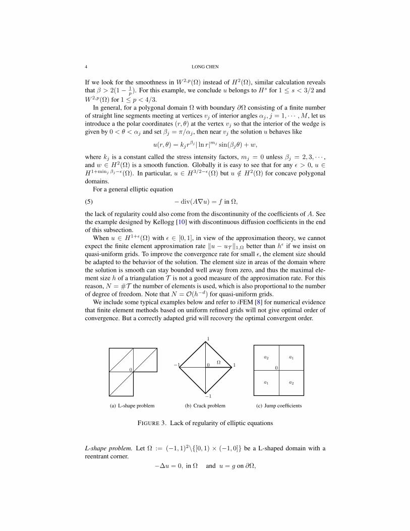
We include some typical examples below and refer to iFEM [8] for numerical evidencethat finite element methods based on uniform refined grids will not give optimal order ofconvergence. But a correctly adapted grid will recovery the optimal convergent order.

Outline Introduction Solve Refine/Coarsen

Lack of Regularity

However the regularity result does not hold in general.

Example (L-shaped Domain Problem)

Let ! := (!1, 1)2\[0, 1)"(!1, 0] and thesolution u satisfies !"u = 0, u|!! = uD .We choose uD such that the exact solution

u(r , !) = r23 sin(

2

3!).

0

FIGURE 1. Patches are similar

1

It is easy to see u # Hs for s < 5/3. In views of the approximationtheory, we cannot expect approximation rate (in H1 norm) betterthan h2/3 if we insist on the quasi-uniform grids.

(a) L-shape problem


Lack of Regularity


Example (Crack Problem)

Let ! = |x | + |y | < 1\0 ! x !1, y = 0 and the solution u satisfies""u = 1, u|!! = uD . We choose uD suchthat the exact solution is

u(r , !) = r12 sin

!

2" 1

4r2.

!0 1!1

1

!1

1

It is easy to see u # Hs for s < 3/2. In views of the approximationtheory, we cannot expect approximation rate (in H1 norm) betterthan h1/2 if we insist on the quasi-uniform grids.

(b) Crack problem


Lack of Regularity


Example (Discontinuous Coe!cients Problem)

Let ! := (!1, 1)2 and consider the equa-tion !" · (A(x)"u) = 0, u|!! = uD , whereA is piecewise constant: in the first andthird quadrants, A = a1I ; in the second andfourth quadrants, A = a2I . The ratio a2/a1

could be very big.

0

a1

a1 a2

a2

FIGURE 1. Patches are similar

1

We can choose parameters such that u # H1+" with 0 < ! $ 1.Again the approximation rate will deteriorate to h" if we still usquasi-uniform grids.

(c) Jump coefficients

FIGURE 3. Lack of regularity of elliptic equations

L-shape problem. Let Ω := (−1, 1)2\[0, 1) × (−1, 0] be a L-shaped domain with areentrant corner.

−∆u = 0, in Ω and u = g on ∂Ω,


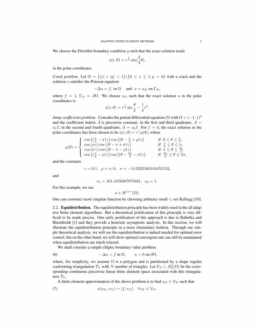
We choose the Dirichlet boundary condition g such that the exact solution reads

u(r, θ) = r23 sin(

2

3θ),

in the polar coordinates.

Crack problem. Let Ω = |x| + |y| < 1\0 ≤ x ≤ 1, y = 0 with a crack and thesolution u satisfies the Poisson equation

−∆u = f, in Ω and u = uD on ΓD,

where f = 1, ΓD = ∂Ω. We choose uD such that the exact solution u in the polarcoordinates is

u(r, θ) = r12 sin

θ

2− 1

4r2.

Jump coefficients problem. Consider the partial differential equation (5) with Ω = (−1, 1)2

and the coefficient matrix A is piecewise constant: in the first and third quadrants, A =a1I; in the second and fourth quadrants, A = a2I . For f = 0, the exact solution in thepolar coordinates has been chosen to be u(r, θ) = rγµ(θ), where

µ(θ) =

cos((π2 − σ)γ

)cos((θ − π

2 + ρ)γ)

if 0 ≤ θ ≤ π2 ,

cos (ργ) cos ((θ − π + σ)γ) if π2 ≤ θ ≤ π,

cos (σγ) cos ((θ − π − ρ)γ) if π ≤ θ ≤ 3π2 ,

cos((π2 − ρ)γ

)cos((θ − 3π

2 − σ)γ)

if 3π2 ≤ θ ≤ 2π,

and the constants

γ = 0.1, ρ = π/4, σ = −14.9225565104455152,

anda1 = 161.4476387975881, a2 = 1.

For this example, we seeu ∈ H1+γ(Ω).

One can construct more singular function by choosing arbitrary small γ; see Kellogg [10].

2.2. Equidistribution. The equidistribution principle has been widely used in the all adap-tive finite element algorithms. But a theoretical justification of this principle is very dif-ficult to be made precise. One early justification of this approach is due to Babuska andRheinboldt [1] and they provide a heuristic asymptotic analysis. In this section, we willillustrate the equidistribution principle in a more elementary fashion. Through our sim-ple theoretical analysis, we will see the equidistribution is indeed needed for optimal errorcontrol, but on the other hand, we will show optimal convergent rate can still be maintainedwhen equidistribution are much relaxed.

We shall consider a simple elliptic boundary value problem

(6) −∆u = f in Ω, u = 0 on ∂Ω,

where, for simplicity, we assume Ω is a polygon and is partitioned by a shape regularconforming triangulation TN with N number of triangles. Let VN ⊂ H1

0 (Ω) be the corre-sponding continuous piecewise linear finite element space associated with this triangula-tion TN .

A finite element approximation of the above problem is to find uN ∈ VN such that

(7) a(uN , vN ) = (f, vN ) ∀vN ∈ VN ,

6 LONG CHEN

where

a(u, v) =

∫Ω

∇u · ∇v dx, and (f, v) =

∫Ω

fv dx.

For this problem, it is well known that for a fixed finite element space VN(8) |u− uN |1,Ω = inf

vN∈VN|u− vN |1,Ω.

We then present a H1 error estimate for linear triangular element interpolation in twodimensions. We note that in two dimensions, the following two embeddings are both valid:

(9) W 2,1(Ω) ⊂W 1,2(Ω) ≡ H1(Ω) and W 2,1(Ω) ⊂ C(Ω).

Given u ∈ W 2,1(Ω), let uI be the linear nodal value interpolant of u on TN . For anytriangle τ ∈ TN , thanks to (9) and the assumption that τ is shape-regular, we have

|u− uI |1,τ . |u|2,1,τ .As a result,

|u− uI |21,Ω .∑τ∈TN

|u|22,1,τ .

To minimize the error, we can try to minimize the right hand side. By Cauchy-Schwarzinequality,

|u|2,1,Ω =∑τ∈TN

|u|2,1,τ ≤ (∑τ∈TN

1)1/2(∑τ∈TN

|u|22,1,τ )1/2 = N1/2(∑τ∈TN

|u|22,1,τ )1/2.

Thus, we have the following lower bound:

(10) (∑τ∈TN

|u|22,1,τ )1/2 ≥ N−1/2|u|2,1,Ω.

The equality holds if and only if

(11) |u|2,1,τ =1

N|u|2,1,Ω.

The condition (11) is hard to be satisfied in general. But we can considerably relax thiscondition to ensure the lower bound estimate (10) is still achieved asymptotically. Therelaxed condition is as follows:

(12) |u|2,1,τ ≤ κτ,N |u|2,1,Ωand

(13)∑τ∈TN

κ2τ,N ≤ c1N−1.

When the above two inequalities hold, we have

|u− uI |1,Ω . N−1/2|u|2,1,Ω.In summary, we have the following theorem.

Theorem 2.1. If TN is a triangulation with at most N triangles and satisfying (12) and(13), then

(14) |u− uN |1 ≤ |u− uI |1,Ω . N−1/2|u|2,1,Ω.


In the above analysis, we see how equidistribution principle plays an important role inachieving asymptotically optimal accuracy for adaptive grids. We would like to furtherelaborate that, in the current setting, equidistribution is indeed a sufficient condition foroptimal error, but by no means this has to be a necessary condition. Namely the equidis-tribution principle can be severely violated but asymptoticly optimal error estimates canstill be maintained. For example, the following mild violation of this principle is certainlyacceptable:

(15) |u|2,1,τ ≤c

N|u|2,1,Ω.

In fact, this condition can be more significantly violated on a finitely many elements τ

(16) |u|2,1,τ ≤c√N|u|2,1,Ω.

It is easy to see if a bounded number of elements satisfy (16) and the rest satisfy (15), theestimate (13) is satisfied and hence the optimal error estimate (14) is still valid.

As we can see that the condition (16) is a very serious violation of equidistributionprinciple, nevertheless, as long as such violations do not occur on too many elements,asymptotically optimal error estimates are still valid. This simple observation is importantfrom both theoretical and practical points of view. The marking strategy proposed by [9]may also be interpreted in this way in its relationship with equidistribution principle.

As it turns out, rigorously speaking, we need a slightly stronger assumption on u(namely smoother than W 2,1(Ω)), for example, u ∈ W 2,p(Ω) 1 for some p > 1. Thisassumption is true for most practical domains; see the discussion in the previous subsec-tion. More precisely, for any p > 1, any N , we have a constructive algorithm [3] to find ashape-regular triangulation TN with O(N) elements such that

|u|2,1,τ ≤ c0N−1|u|2,p,Ω.As a result, since |u− uT |1,Ω ≤ |u− uI |1,Ω, we have the following error estimate

(17) |u− uT |1,Ω . N−1/2|u|2,p,Ω.which is asymptotically best possible for an isotropic triangulation with O(N) elements.Recent works have shown that the estimate (17) can be practically realized [6, 7, 13, 18]by using appropriate a posteriori error estimates below.

3. NEWEST VERTEX BISECTION

In this section we shall give a brief introduction of the newest vertex bisection. We referto [12, 19, 6] for detailed description of the newest vertex bisection refinement procedureand especially [6] for the control of the number of elements added by the completionprocess.

We first recall two important properties of triangulations. A triangulation Th (also in-dicated by mesh or grid) of Ω ⊂ R2 is a decomposition of Ω into a set of triangles. It iscalled conforming if the intersection of any two triangles τ and τ ′ in Th either consists ofa common vertex xi, edge E or empty. An edge of a triangle is called non-conforming ifthere is a vertex in the interior of that edge and that interior vertex is called hanging node.See Fig. 3 (b) for an example of non-conforming triangles and hanging nodes. We wouldlike to keep the conformity of the triangulations.

1it actually suffices if M(∇2u) ∈ L1(Ω), where M(f) is the Hardy-Littlewood maximal function of f

8 LONG CHEN

A triangulation Th is shape regular if

(18) maxτ∈Th

diam(τ)2

|τ | ≤ σ

where diam(τ) is the diameter of τ and |τ | is the area of τ . A sequence of triangulationTk, k = 0, 1, · · · is called uniform shape regular if σ in (18) is independent with k.

The shape regularity of triangulations assures that angles of the triangulation remainsbounded away from 0 and π which is important to control the interpolation error in H1

norm and the condition number of the stiffness matrix. We also want to keep this propertyof the triangulations.

After we marked a set of triangles to be refined, we need to carefully design the rulefor dividing the marked triangles such that the refined mesh is still conforming and shaperegular. Such refinement rules include red and green refinement [4], longest edge bisection[16, 15] and newest vertex bisection [17]. We shall restrict ourself to the newest vertexbisection method since it will produce nested finite element spaces and relatively easier togeneralize to high dimensions.

Given an initial shape regular triangulation T0 of Ω, we assign to each τ ∈ T0 exactlyone vertex called the newest vertex. The opposite edge of the newest vertex is calledrefinement edge. One such initial labeling is to use the longest edge of each triangle (witha tie breaking scheme for edges of equal length). The rule of the newest vertex bisectionincludes:

(1) a triangle is divided to two new children triangles by connecting the newest vertexto the midpoint of the refinement edge;

(2) the new vertex created at a midpoint of a refinement edge is assigned to be thenewest vertex of the children.

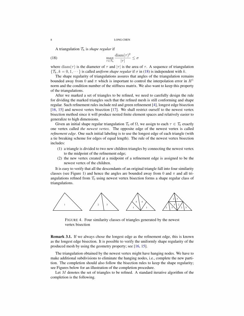
It is easy to verify that all the descendants of an original triangle fall into four similarityclasses (see Figure 1) and hence the angles are bounded away from 0 and π and all tri-angulations refined from T0 using newest vertex bisection forms a shape regular class oftriangulations.

CHAPTER 1. CONVERGENCEOF ADAPTIVE FINITE ELEMENTMETHODS 10

Figure 1.1: Edges in bold case are bases

1 2 3

1 1

4 4

2 3 2 3

3 2

2 3

Figure 1.2: Four similarity classes of triangles generated by the newest vertex bisection

1.2 Preliminaries

In this section we shall present some preliminaries needed for the convergence analysis of the

adaptive finite element methods. We first discuss the newest vertex bisection which is the rule

we used to divide the triangles. We then present a quasi-interpolation operator which is crucial

to prove the upper bound of residual type a posteriori error estimator.

Newest vertex bisection

In this subsection we give a brief introduction of the newest vertex bisection and mainly concern

the number of elements added by the completion process. We refer to [31, 42] and [11] for

detailed description of the newest vertex bisection refinement procedure.

Given an initial shape regular triangulation T0 of !, it is possible to assign to each ! ! T0

exactly one vertex called peak or the newest vertex. The opposite edge of the peak is called base.

The rule of the newest vertex bisection includes: 1) a triangle is divided to two new children

triangles by connecting the peak to the midpoint of the base; 2) the new vertex created at a

midpoint of a base is assigned to be the peak of the children. Sewell [39] showed that all the

decendants of an original triangle fall into four similarity classes (see Figure 1.2) and hence the

angles are bounded away from 0 and ".

To generate a triangulation Tk+1 from previous one Tk, we first mark some of the triangles of

Tk according to some marking strategy and subdivide the marked triangles using newest vertex

bisection to get T !k+1. The new partition T !

k+1 might have hanging nodes. We make additional

subdivisions to eliminate the hanging nodes i.e. complete the new partition. The completion is

made by dividing triangles using the designated peaks and base points. Tk+1 will be defined as

FIGURE 4. Four similarity classes of triangles generated by the newestvertex bisection

Remark 3.1. If we always chose the longest edge as the refinement edge, this is knownas the longest edge bisection. It is possible to verify the uniformly shape regularity of theproduced mesh by using the geometry property; see [16, 15].

The triangulation obtained by the newest vertex might have hanging nodes. We have tomake additional subdivisions to eliminate the hanging nodes, i.e., complete the new parti-tion. The completion should also follow the bisection rules to keep the shape regularity;see Figures below for an illustration of the completion procedure.

Let M denotes the set of triangles to be refined. A standard iterative algorithm of thecompletion is the following.


(a) Bisect a triangle (b) Completion

FIGURE 1. Newest vertex bisection

(a) Bisect a triangle

0 1 2 3 4

0

1

2

(b) Completion


1

(a) An initial triangulation




0 1 2 3 4

0

1

2

(b) Completion


1

(b) Refine two triangles producing anon-conforming edge




0 1 2 3 4

0

1

2

(b) Completion


1

(c) Refine one triangle to obtain a con-forming triangulation

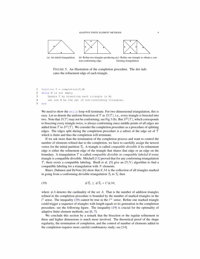
FIGURE 5. An illustration of the completion procedure. The dot indi-cates the refinement edge of each triangle.

1 function T = completion(T,M)

2 while M is not empty

3 Update T by bisecting each triangle in M;

4 Let now M be the set of non-conforming triangles.

5 end

We need to show the while loop will terminate. For two dimensional triangulation, this iseasy. Let us denote the uniform bisection of T as D(T ), i.e., every triangle is bisected intotwo. Note thatD(T ) may not be conforming; see Fig 3 (b). ButD2(T ), which correspondsto bisecting every triangle twice, is always conforming since middle points of all edges areadded from T toD2(T ). We consider the completion procedure as a procedure of splittingedges. The edges split during the completion procedure is a subset of the edge set of Twhich is finite and thus the completion will terminate.

If we ask more than the termination of the completion process and want to control thenumber of elements refined due to the completion, we have to carefully assign the newestvertex for the initial partition T0. A triangle is called compatible divisible if its refinementedge is either the refinement edge of the triangle that shares that edge or an edge on theboundary. A triangulation T is called compatible divisible or compatible labeled if everytriangle is compatible divisible. Mitchell [11] proved that for any conforming triangulationT , there exists a compatible labeling. Biedl et al. [5] give an O(N) algorithm to find acompatible labeling for a triangulation with N elements.

Binev, Dahmen and DeVore [6] show that ifM is the collection of all triangles markedin going from a conforming divisible triangulation T0 to Tk then

(19) #Tk ≤ #T0 + C#M,

where #A denotes the cardinality of the set A. That is the number of addition trianglesrefined in the completion procedure is bounded by the number of marked triangles in thel1 sense. The inequality (19) cannot be true in the l∞ sense. Refine one marked trianglecould trigger a sequence of triangles with length equals to its generation in the completionprocedure; see the following figure. The inequality (19) is crucial for the optimality ofadaptive finite element methods; see [6, 7].

We conclude this section by a remark that the bisection or the regular refinement inthree and higher dimensions is much more involved. The theoretical proof of the shaperegularity, the termination of completion, and the control of number of elements added inthe completion requires more careful combinatory study; see [14].

10 LONG CHEN

4. RESIDUAL TYPE A POSTERIOR ERROR ESTIMATE

In this section we consider the linear finite element approximation of the Poisson

(20) −∆u = f in Ω, u = 0 on ∂Ω,

and shall derive a residual type a posterior error estimate of the error |u − uT |1,Ω. Othertypes of a posterior error estimator include: recovery type; solving local problem; solvinga dual problem; superconvergence result.

4.1. A local and stable quasi-interpolation. To define a function in the linear finite el-ement space VT , we only need to assigned the value at interior vertices. For a vertexxi ∈ N (T ), recall that Ωi consists of all simplexes sharing this vertex and for an elementΩτ = ∪xi∈τΩi. Instead of using nodal values of the object function, we can use its integralover Ωi.

For an interior vertex xi, we define a constant function on Ωi byAiu = |Ωi|−1∫

Ωiu(x)dx.

To incorporate the boundary condition, when xi ∈ ∂Ω, we defineAiu = 0. We then definethe averaged interpolation ΠT : L1 7→ VT by

ΠT u =∑

xi∈N (T )

Ai(u)ϕi.

Lemma 4.1. For u ∈ H1(Ωτ ), we have the error estimate

‖u−ΠT u‖0,τ . hτ |u|1,Ωτ .

Proof. For interior vertices, we use average type Poincare inequality, to obtain

(21) ‖u−Aiu‖0,Ωi ≤ Chτ |u|1,Ωi ,and for boundary vertices, we use Poincare-Friedriches since then u|∂Ωi∩∂Ω = 0 and theRd−1 Lebesgue measure of the set ∂Ωi ∩ ∂Ω is non-zero. The constant C in the equality(21) can be chosen as one independent with Ωi since the mesh is shape regular. Then weuse the partition of unity

∑d+1i=1 ϕi = 1 restricted to one element τ to write∫

τ

|u−ΠT u|2 =

∫τ

∣∣∣ d+1∑i=1

(u−Aiu)ϕi

∣∣∣2 dx .d+1∑i=1

∫Ωi

|u−Aiu|2 dx

. hτ

d+1∑i=1

∫Ωi

|∇u|2 dx . Ch2τ

∫Ωτ

|∇u|2 dx.

We now prove that ΠT is stable in H1 norm. Let us introduce another average oper-ator Aτ : the L2 projection to the piecewise constant function spaces on Th: (Aτu)|τ =|τ |−1

∫τu(x)dx.

Lemma 4.2. For u ∈ H1(Ωτ ), we have the stability

|ΠT u|1,τ . |u|1,Ωτ .

Proof. Using Poincare inequality it is easy to see

‖u−Aτu‖0,τ . hτ |u|1,τ .


We use the inverse inequality and first order approximation property of Aτ and ΠT toobtain

|ΠT u|1,τ = |ΠT u−Aτu|1,τ ≤ h−1τ ‖ΠT u−Aτu‖0,τ

≤ h−1τ

(‖u−ΠT u‖0,τ + ‖u−Aτu‖0,τ

). |u|1,Ωτ .

Theorem 4.3. For u ∈ H1(Ω), the quasi-interpolant ΠT u satisfies(∑τ∈T‖h−1(u−ΠT u)‖20,τ + ‖∇(u−ΠT u)‖20,τ

)1/2

. |u|1,Ω.

4.2. Upper bound. The equidistribution principle suggested us to equidistribute the quan-tity |u|2,1,τ . It is, however, not computable since u is unknown. One may want to approx-imate it by |uT |2,1,τ . For linear finite element function uT , we have |uT |2,1,τ = 0 andthus no information of |u|2,1,τ will be obtained in this way. More rigorously, the derivativeof the piecewise constant vector function ∇uT will be delta distributions on edges withmagnitude as the jump of ∇uT across the edge. On the other hand, ∆u ∈ L2(Ω) implies∇u ∈ H(div; Ω), i.e.,∇u ·ne is continuous at an edge e where ne is a unit norm vector ofe. For the finite element approximation uT ∈ VT , it is easy to see ∇uT · ne is not contin-uous (although the tangential derivative∇uT · te is). The discontinuity of norm derivativeacross edges can be used to measure the error∇u−∇uT .

More precisely, let ET denote the set of all interior edges, for each interior edge e ∈ ET ,we fix a unit norm vector ne. Let τ1 and τ2 be two triangles sharing the edge e. The jumpof flux across e is defined as

[∇uT · ne] = ∇uT · ne|τ1 −∇uT · ne|τ2 .

We define h as a piecewise constant function on T , that is for each element τ ∈ T ,

(22) h|τ = hτ = |τ |1/2.

We also define a piecewise constant function on ET as

(23) h|e = he := (hτ1 + hτ2)/2,

where e = τ1 ∩ τ2 is the common edge of two triangles. We provide a posterior errorestimate for the Poisson equation with homogenous Dirichlet boundary condition belowand refer to [19] for general elliptic equations and mixed boundary conditions.

Theorem 4.4. For a given triangulation T , let uT be the linear finite element approxi-mation of the solution u of the Poisson equation. Then there exists a constant C1 > 0depending only on the shape regularity of T such that

(24) |u− uT |1 ≤ C1

(∑τ∈T‖hf‖20,τ +

∑e∈ET

‖h1/2[∇uT · ne]‖20,e)1/2

.

12 LONG CHEN

Proof. For any w ∈ H10 (Ω) and any wT ∈ VT , we have

a(u− uT , w)

= a(u− uT , w − wT )

=∑τ∈T

∫τ

∇(u− uT ) · ∇(w − wT ) dx

=∑τ∈T

∫τ

−∆(u− uT )(w − wT ) dx +∑τ∈T

∫∂τ

∇(u− uT ) · n(w − wT ) dS

=∑τ∈T

∫τ

f(w − wT ) dx +∑e∈Eh

∫e

[∇uT · ne](w − wT ) dS

≤∑τ∈T‖hf‖0,τ‖h−1(w − wT )‖0,τ +

∑e∈Eh

‖h1/2[∇uT · ne]‖0,e‖h−1/2(w − wT )‖0,e

.

(∑τ∈T‖hf‖20,τ +

∑e∈ET

‖h−1/2[∇uT · ne]‖20,e

)1/2

(∑τ∈T‖h−1(w − wT )‖20,τ + ‖∇(w − wT )‖20,τ

)1/2

.

In the last step, we have used the trace theorem with the scaling argument to get

‖w − wT ‖0,e . h−1/2τ ‖w − wT ‖0,τ + h1/2

τ ‖∇(w − wT )‖0,τ .Now chose wT = ΠT w by the quasi-interpolation operator introduced in Theorem 4.3, wehave

(25)

(∑τ∈T‖h−1(w − wT )‖20,τ + ‖∇(w − wT )‖20,τ

)1/2

. |w|1,Ω.

Then we end with

|u− uT |1 = supw∈H1

0 (Ω)

a(u− uT , w)

|w|1.(∑τ∈T‖hf‖20,τ +

∑e∈ET

‖h1/2[∇uT · ne]‖20,e)1/2

.

To guide the local refinement, we need to have an element-wise (or edge-wise) errorindicator. For any τ ∈ T and any vT ∈ VT , we define

(26) η(vT , τ) =(‖hf‖20,τ +

∑e∈∂τ

‖h1/2[∇vT · ne]‖20,e)1/2

.

For a subsetMT ⊆ T , we define

η(vT ,MT ) =[∑

τ

η2(vT , τ)]1/2

.

With these notation, the upper bound (24) can be simply written as

(27) |u− uT |1,Ω ≤ C1η(uT , T ).

Remark 4.5. The local version of the upper bound (27)

|u− uT |1,τ ≤ C1η(uT , τ)

does not hold in general.


4.3. Lower bound. We shall derive a lower bound of the error estimator η through thefollowing exercises. The technique is developed by Verfurth [19] and known as bubblefunctions. Let u be the solution of Poisson equation −∆u = f with homogeneous Dirich-let boundary condition and uT be the linear finite element approximation of u based on ashape regular and conforming triangulation T .

Exercise 4.6. (1) For a triangle τ , we denote Vτ = fτ ∈ L2(τ) | fτ = constantequipped with L2 inner product. Let λi(x), i = 1, 2, 3 be the barycenter coordi-nates of x ∈ τ , and let bτ = λ1λ2λ3 be the bubble function on τ . We defineBτfτ = fτ bτ .

Prove that Bτ : Vτ 7→ V = H10 (Ω) is bounded in L2 and H1 norm:

‖Bτfτ‖0,τ = C‖fτ‖0,τ , and ‖∇(Bτfτ )‖0,τ . h−1τ ‖fτ‖0,τ .

(2) Using (1) to prove that

‖hfτ‖0,τ . |u− uT |1,τ + ‖h(f − fτ )‖0,τ .

(3) For an interior edge e, we define Ve = ge ∈ L2(E) | ge = constant. Suppose ehas end points xi, and xj , we define be = λiλj andBe : Ve 7→ V byBege = gebe.

Let ωe denote two triangles sharing e. Prove that(a) ‖ge‖0,e = C‖Bege‖0,e,(b) ‖Bege‖0,ωe . h1/2

e ‖ge‖0,e and,

(c) ‖∇(Bege)‖0,ωe . h−1/2e ‖ge‖0,e.

(4) Using (3) to prove that

‖h1/2[∇uT · ne]‖0,e . ‖hf‖0,ωe + |u− uT |1,ωe .

(5) Using (1) and (4) to prove the lower bound of the error estimator. There exists aconstant C2 depending only on the shape regularity of the triangulation such thatfor any piecewise constant approximation fτ of f ∈ L2,

C2η2(uT , T ) ≤ |u− uT |21,Ω +

∑τ∈Th

‖h(f − fτ )‖2τ .

5. CONVERGENCE

Standard adaptive finite element methods (AFEM) based on the local mesh refinementcan be written as loops of the form

(28) SOLVE → ESTIMATE→ MARK → REFINE.

Starting from an initial triangulation T0, to get Tk+1 from Tk we first solve the equation toget uk based on Tk (the indices of second order like uTk will be contracted as uk). The erroris estimated using uk and Tk and used to mark a set of of triangles in Tk. Marked trianglesand possible more neighboring triangles are refined in such a way that the triangulation isstill shape regular and conforming.

14 LONG CHEN

5.1. Algorithm. The step SOLVE is discussed in Chapter: Iterative method, where effi-cient iterative methods including multigrid and conjugate gradient methods is studied indetail. Here we assume that the solutions of the finite dimensional problems can be solvedto any accuracy efficiently.

The a posteriori error estimators are an essential part of the ESTIMATE step. We havegiven one in the previous section and will discuss more in the next section.

The a posteriori error estimator is split into local error indicators and they are thenemployed to make local modifications by dividing the elements whose error indicator islarge and possibly coarsening the elements whose error indicator is small. The way wemark these triangles influences the efficiency of the adaptive algorithm. The traditionalmaximum marking strategy proposed in the pioneering work of Babuska and Vogelius [2]is to mark triangles τ∗ such that

η(uT , τ∗) ≥ θmax

τ∈Tη(uT , τ), for some θ ∈ (0, 1).

Such marking strategy is designed to evenly equi-distribute the error. Based our relaxationof the equidistribution principal, we may leave some exceptional elements and focus onthe overall amounts of the error. This leads to the bulk criterion firstly proposed by Dorfler[9] in order to prove the convergence of the local refinement strategy. With such strategy,one defines the marking setMT ⊂ T such that

(29) η2(uT ,MT ) ≥ θ η2(uT , T ), for some θ ∈ (0, 1).

We shall use Dorfler marking strategy in the proof.After choosing a set of marked elements, we need to carefully design the rule for divid-

ing the marked triangles such that the mesh obtained by this dividing rule is still conform-ing and shape regular. Such refinement rules include red and green refinement [4], longestrefinement [16, 15], and newest vertex bisection [17, 12]. In addition we also would liketo control the number of elements added to ensure the optimality of the refinement. To thisend we shall use the newest vertex bisection discussed in the previous section.

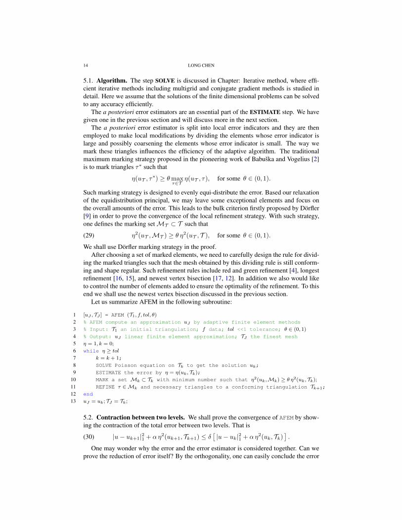
Let us summarize AFEM in the following subroutine:

1 [uJ , TJ ] = AFEM (T1, f, tol, θ)2 % AFEM compute an approximation uJ by adaptive finite element methods

3 % Input: T1 an initial triangulation; f data; tol <<1 tolerance; θ ∈ (0, 1)

4 % Output: uJ linear finite element approximation; TJ the finest mesh

5 η = 1, k = 0;

6 while η ≥ tol7 k = k + 1;

8 SOLVE Poisson equation on Tk to get the solution uk;

9 ESTIMATE the error by η = η(uk, Tk);

10 MARK a set Mk ⊂ Tk with minimum number such that η2(uk,Mk) ≥ θ η2(uk, Tk);

11 REFINE τ ∈Mk and necessary triangles to a conforming triangulation Tk+1;

12 end

13 uJ = uk; TJ = Tk;

5.2. Contraction between two levels. We shall prove the convergence of AFEM by show-ing the contraction of the total error between two levels. That is

(30) |u− uk+1|21 + αη2(uk+1, Tk+1) ≤ δ[|u− uk|21 + αη2(uk, Tk)

].

One may wonder why the error and the error estimator is considered together. Can weprove the reduction of error itself? By the orthogonality, one can easily conclude the error


is non-increasing, i.e.|u− uk+1|1 ≤ |u− uk|1.

The equality could hold if the refinement did not introduce interior nodes for triangles andedges; see Example 3.6 and 3.7 in [13]. A close look reveals that when the solution doesnot change, the error estimator η will be reduced by a factor less than one due to the changeof mesh size and the Dorfler marking strategy.

To prove (30) let us begin with the following properties of the error estimator and errorin consecutive levels Tk and Tk+1.

Lemma 5.1. Given a θ ∈ (0, 1), let Tk+1 be a conforming and shape regular triangula-tion which is refined from a conforming and shape regular triangulation Tk using Dorflermarking strategy (29). Let uk+1 and uk be solutions of (4) in Vk+1 and Vk, respectively.Then we have

(1) orthogonality: |u− uk+1|21 = |u− uk|21 − |uk+1 − uk|21;

(2) upper bound: |u− uk|21 ≤ C1η2(uk, Tk) for some constant C1 depending only on

the shape regularity of T ;

(3) continuity of error estimator: for any ε > 0, there exists a constant Cε such that

η2(uk+1, Tk+1) ≤ (1 + ε)η2(uk, Tk+1) + Cε|uk+1 − uk|21;

(4) contraction of error estimator: η2(uk, Tk+1) ≤ ρ η2(uk, Tk) for some ρ ∈ (0, 1)depending only on the shape regularity of Tk and the parameter θ used in theDorfler marking strategy.

Proof. (1) is trivial since uk+1 is theH1 projection and uk+1−uk ∈ Vk+1 by the nestnessof Tk and Tk+1. (2) has been proved in the previous section.

We now prove (3). The part contains element-wise residual ‖hf‖ is unchanged sincewe do not change the triangulation. For each e ∈ ET , let τ ∈ T such that e ∈ ∂τ . Fromthe triangle inequality and the fact∇(uk+1 − uk) is piecewise constant, we have

‖h1/2[∇uk+1 · ne]‖0,e ≤ ‖h1/2[∇uk · ne]‖0,e + ‖h1/2[∇(uk+1 − uk) · ne]‖0,e,≤ ‖h1/2[∇uk · ne]‖0,e + C|uk+1 − uk|1,τ .

Square both sides, apply the Young’s inequality 2ab ≤ εa2 + ε−1b2 and sum all edges toget the desired inequality.

To prove (4), we study in detail the change of the error estimator due to the bisection ofa triangle. Suppose τ is bisected to τ1 and τ2. We shall first prove element-wise contractionof error indicator: There exists a number ρ ∈ (0, 1) depending only on the shape regularityof Tk such that

(31) η2(uk, τ1) + η2(uk, τ2) ≤ ρ η2(uk, τ).

To distinguish the difference mesh size function, we use hk+1 and hk to denote the meshsize function defined on Tk and Tk+1, respectively. Thanks to our definition, h2

k+1,τi=

|τi| = 1/2|τ | = 1/2h2k,τ . The part involving element residual is reduced by one half:

‖hk+1f‖2τ1 + ‖hk+1f‖2τ2 =1

2‖hkf‖2τ .

For the jump of gradient on the edges, an important observation is that [∇uk · ne] = 0for the new created edge inside τ . For other edges on the boundary of τ , he is reduced bya factor due to the definition of he and the shape regularity of the triangulation while the

16 LONG CHEN

jump [∇uk · ne] remains unchanged. So∑e∈∂τ ‖h1/2[∇vT · ne]‖20,e is also reduced by a

factor strictly less than one.We then move the global version. Recall thatMk ⊂ Tk is the marked set. We may need

to refine more triangles to recover the conformity of the triangulation and thus denote theset of refined triangles byMk. SinceMk ⊆ Mk, we have η2(uk,Mk) ≥ θη2(uk, Tk).We useMk+1 ⊂ Tk+1 to denote the set of triangles obtained by refinement of that inMk.Obviously Tk\Mk = Tk+1\Mk+1 are untouched triangles. We then have

η2(uk, Tk+1) = η2(uk, Tk+1\Mk+1) + η2(uk,Mk+1)

≤ η2(uk, Tk\Mk) + ρ η2(uk,Mk)

= η2(uk, Tk)− (1− ρ) η2(uk,Mk)

≤ η2(uk, Tk)− θ(1− ρ) η2(uk, Tk)

=[1− θ(1− ρ)

]η2(uk, Tk).

We obtain (4) with ρ = 1− θ(1− ρ) ∈ (0, 1).

We are in the position to prove the contraction result.

Theorem 5.2. Given a θ ∈ (0, 1), let Tk+1 be a conforming and shape regular triangula-tion which is refined from a conforming and shape regular triangulation Tk using Dorflermarking strategy (29). Let uk+1 and uk be solutions of (4) in Vk+1 and Vk, respectively.Then there exist constants δ ∈ (0, 1) and α depending only on θ and the shape regularityof Tk such that

(32) |u− uk+1|21 + αη2(uk+1, Tk+1) ≤ δ[|u− uk|21 + αη2(uk, Tk)

].

Proof. Let ρ ∈ (0, 1) be the constant in Lemma 5.1 (4). Since ρ ∈ (0, 1), we can chooseε ∈ (0, 1) and small enough such that ρ(1 + ε) < 1 and let α = C−1

ε . Let δ be a numberin (0, 1) whose value will be clear in a moment. We then have

|u− uk+1|21 + αη2(uk+1, Tk+1)

=|u− uk|21 + αη2(uk+1, Tk+1)− |uk+1 − uk|21≤δ|u− uk|21 + (1− δ)|u− uk|21 + α(1 + ε) η2(uk, Tk+1)

≤δ|u− uk|21 + (1− δ)C1η2(uk, Tk) + αρ(1 + ε) η2(uk, Tk)

≤δ[|u− uk|21 +

(1− δ)C1 + αρ(1 + ε)

δη2(uk, Tk)

].

In the first step, we simply add αη2(uk+1, Tk+1) to the orthogonality identity (Lemma 5.1(1)). Then we split |u−uk|21 and apply the continuity of error estimator (Lemma 5.1 (3)) tocancel |uk+1−uk|21. Next we apply the upper bound (Lemma 5.1 (3)) to (1−δ)|u−uk|21 andthe reduction of η (Lemma 5.1 (4)). The last step is a simple rearrangement of constants.

This suggests us to choose δ such that

α =(1− δ)C1 + αρ(1 + ε)

δ.

Namely

(33) δ =C1 + αρ(1 + ε)

C1 + α.

Recall that we choose ε such that ρ(1 + ε) < 1, so δ ∈ (0, 1). The desired result (32) thenfollows.


5.3. Convergence. As a consequence of the contraction of the total error between twolevels, we can prove AFEM will stop in finite steps for a given tolerance tol and producea convergent approximation uJ based on an adaptive grid TJ . We refer to [18, 7] for theanalysis of complexity which is much more involved.

Theorem 5.3. Let uk and T be the solution and triangulation obtained in the k-th loop inthe algorithm AFEM, then there exist constants δ ∈ (0, 1) and α depending only on θ andthe shape regularity of T0 such that

(34) |u− uk|21 + αη2(uk, Tk) ≤ C0δk,

and thus the algorithm AFEM will terminate in finite steps.

REFERENCES

[1] I. Babuska and W. C. Rheinboldt. Error estimates for adaptive finite element computations. SIAM J. Numer.Anal., 15:736–754, 1978.

[2] I. Babuska and M. Vogelius. Feeback and adaptive finite element solution of one-dimensional boundaryvalue problems. Numer. Math., 44:75–102, 1984.

[3] C. Bacuta, L. Chen, and J. Xu. Equidistribution and optimal approximation class. In M. W. O. X. J. Bank,Randolph Holst, editor, Domain Decomposition Methods in Science and Engineering XX, volume 91, pages3–14, 2013.

[4] R. E. Bank, A. H. Sherman, and A. Weiser. Refinement algorithms and data structures for regular local meshrefinement. In Scientific Computing, pages 3–17. IMACS/North-Holland Publishing Company, Amsterdam,1983.

[5] T. C. Biedl, P. Bose, E. D. Demaine, and A. Lubiw. Efficient algorithms for Petersen’s matching theorem. J.Algorithms, 38(1):110–134, 2001.

[6] P. Binev, W. Dahmen, and R. DeVore. Adaptive finite element methods with convergence rates. Numer.Math., 97(2):219–268, 2004.

[7] J. M. Cascon, C. Kreuzer, R. H. Nochetto, and K. G. Siebert. Quasi-optimal convergence rate for an adaptivefinite element method. SIAM J. Numer. Anal., 46(5):2524–2550, 2008.

[8] L. Chen. iFEM: An Integrated Finite Element Methods Package in MATLAB. Technical Report, Universityof California at Irvine, 2009.

[9] W. Dorfler. A convergent adaptive algorithm for Poisson’s equation. SIAM J. Numer. Anal., 33:1106–1124,1996.

[10] R. B. Kellogg. On the Poisson equation with intersecting interface. Appl. Aanal., 4:101–129, 1975.[11] W. F. Mitchell. Unified Multilevel Adaptive Finite Element Methods for Elliptic Problems. PhD thesis, Uni-

versity of Illinois at Urbana-Champaign, 1988.[12] W. F. Mitchell. A comparison of adaptive refinement techniques for elliptic problems. ACM Trans. Math.

Softw. (TOMS) archive, 15(4):326 – 347, 1989.[13] P. Morin, R. H. Nochetto, and K. G. Siebert. Convergence of adaptive finite element methods. SIAM Rev.,

44(4):631–658, 2002.[14] R. H. Nochetto, K. G. Siebert, and A. Veeser. Theory of adaptive finite element methods: an introduction. In

R. A. DeVore and A. Kunoth, editors, Multiscale, Nonlinear and Adaptive Approximation. Springer, 2009.[15] M. C. Rivara. Design and data structure for fully adaptive, multigrid finite element software. ACM Trans.

Math. Soft., 10:242–264, 1984.[16] M. C. Rivara. Mesh refinement processes based on the generalized bisection of simplices. SIAM J. Numer.

Anal., 21:604–613, 1984.[17] E. G. Sewell. Automatic Generation of Triangulations for Piecewise Polynomial Approximation. PhD thesis,

Purdue Univ., West Lafayette, Ind., 1972.[18] R. Stevenson. Optimality of a standard adaptive finite element method. Found. Comput. Math., 7(2):245–

269, 2007.[19] R. Verfurth. A Review of A Posteriori Error Estimation and Adaptive Mesh Refinement Tecniques. B. G.

Teubner, 1996.

adaptive finite element methods - …chenlong/226/ch4afem.pdf · adaptive finite element methods 3...

Documents