IOP PUBLISHING INVERSE PROBLEMS

Inverse Problems 24 (2008) 034011 (22pp) doi:10.1088/0266-5611/24/3/034011

Adaptive finite element methods for the solution ofinverse problems in optical tomography

Wolfgang Bangerth1 and Amit Joshi2

1 Department of Mathematics, Texas A&M University, College Station TX 77843-3368, USA2 Department of Radiology, Baylor College of Medicine, Houston TX 77030, USA

E-mail: bangerth@math.tamu.edu and amitj@bcm.edu

Received 16 July 2007, in final form 12 February 2008Published 23 May 2008Online at stacks.iop.org/IP/24/034011

AbstractOptical tomography attempts to determine a spatially variable coefficient inthe interior of a body from measurements of light fluxes at the boundary.Like in many other applications in biomedical imaging, computing solutionsin optical tomography is complicated by the fact that one wants to identify anunknown number of relatively small irregularities in this coefficient at unknownlocations, for example corresponding to the presence of tumors. To recoverthem at the resolution needed in clinical practice, one has to use meshes that,if uniformly fine, would lead to intractably large problems with hundreds ofmillions of unknowns. Adaptive meshes are therefore an indispensable tool.In this paper, we will describe a framework for the adaptive finite elementsolution of optical tomography problems. It takes into account all steps startingfrom the formulation of the problem including constraints on the coefficient,outer Newton-type nonlinear and inner linear iterations, regularization, and inparticular the interplay of these algorithms with discretizing the problem ona sequence of adaptively refined meshes. We will demonstrate the efficiencyand accuracy of these algorithms on a set of numerical examples of clinicalrelevance related to locating lymph nodes in tumor diagnosis.

(Some figures in this article are in colour only in the electronic version)

1. Introduction

Fluorescence-enhanced optical tomography is a recent and highly active area in biomedicalimaging research. It attempts to reconstruct interior body properties using light in the red andinfrared range in which biological tissues are highly scattering but not strongly absorbing.It is developed as a tool for imaging up to depths of several centimeters, which includes in

0266-5611/08/034011+22$30.00 © 2008 IOP Publishing Ltd Printed in the UK 1

Inverse Problems 24 (2008) 034011 W Bangerth and A Joshi

particular important applications to breast and cervix cancer detection and staging, lymphnode imaging, but also imaging of the brain of newborns through the skull.

Optical tomography addresses a number of shortcomings of established imagingtechniques. Most currently available techniques only image secondary effects of tumorssuch as calcification of blood vessels (x-rays), density and stiffness differences (ultrasound)or water content (MRI) of tissues. While such effects are often associated with tumors, theyare not always, and frequently lead to both false positive and false negative assessments. Inaddition, x-ray imaging uses ionizing radiation and is therefore harmful and potentially cancerinducing. In contrast, optical tomography is a method that (i) does not use harmful radiation,and (ii) can be made specific to tumors on the molecular level, distinguishing proteins andother molecules that are only expressed in certain tissues we are interested in (for exampletumor cells, or lymph nodes if the goal is to track the spread of a tumor).

The idea behind optical tomography [4] is to illuminate the tissue surface with a knownlaser source. The light will diffuse and be absorbed in the tissue. By observing the lightflux exiting the tissue surface, one hopes to recover the spatial structure of absorption andscattering coefficients inside the sample, which in turn is assumed to coincide with anatomicaland pathological structures. For example, it is known that hemoglobin concentration, bloodoxygenation levels and water content affect optical tissue properties, all of which are correlatedwith the presence of tumors. As a result diffuse optical tomography (DOT) can uniquely imagethe in vivo metabolic environment [23, 36, 37, 77].

However, DOT has been recognized as a method that is hard to implement because it doesnot produce a very large signal-to-noise ratio. This follows from the fact that a relatively smalltumor, or one that does not have a particularly high absorption contrast, does not producemuch dimming of the light intensity on the surface, in particular in reflection geometry, i.e.where illumination and measurement surfaces coincide. Another drawback of DOT is that itis non-specific: it detects areas of high light absorption, but does not distinguish the reasonsfor absorption; for example, it cannot distinguish between naturally dark tissues as comparedto invading dark diseased tissues.

During the last decade, a number of approaches have been developed that attempt to avoidthese drawbacks. One is fluorescence-enhanced optical tomography, in which a fluorescentdye (or ‘fluorophore’) is injected that specifically targets certain tissue types, for exampletumor or lymph node cells. The premise is that it is naturally washed out from the rest of thetissue. If the dye is excited using light of one wavelength, then we will get a fluorescent signalat a different wavelength, typically in the infrared, from areas in which dye is present (i.e.where the tumor or a lymph node is). In other words, if we illuminate the skin with a red laser,light will travel into the tissue, be absorbed by the dye, and will be re-emitted at a differentwavelength (in the infrared range). This secondary light is then detected again at the skin:here, a bright infrared spot on the surface indicates the presence of a high dye concentrationunderneath, which is then indicative of the presence of the tissue kind the dye is specific to.

Since the signal is the presence of a different kind of light, not a faint dimming of theincident light intensity, the signal to noise ratio of fluorescence optical tomography is muchbetter than in DOT. It is also much better than, for example, in positron emission tomography(PET) because dyes can be excited millions or billions of times per second, each time emittingan infrared photon. In addition, the specificity of dyes can be used for molecularly targetedimaging, i.e. we can really image the presence of diseased cells, not only secondary effects.

In the past, fluorescence tomography schemes have been proposed for pre-clinical smallanimal imaging applications [31] as well as for the clinical imaging of large tissue volumes[25, 28, 30, 43, 57, 58, 61, 67–69, 72, 74, 76, 81]. Typical fluorescence optical tomographyschemes employ iterative image reconstruction techniques to determine the fluorescence yield

2

Inverse Problems 24 (2008) 034011 W Bangerth and A Joshi

or lifetime map in the tissue from boundary fluorescence measurements. A successful clinicallyrelevant fluorescence tomography system will have the following attributes: (i) rapid dataacquisition to minimize patient movement and discomfort, (ii) accurate and computationallyefficient modeling of light propagation in large tissue volumes and (iii) a robust imagereconstruction strategy to handle the ill-posedness introduced by the diffuse propagationof photons in tissue and the scarcity of data.

From a computational perspective, the challenge in optical tomography—as in many othernonlinear imaging modalities—is to reach the clinically necessary resolution within acceptablecompute times. To illustrate this, consider that the typical volume under interrogation inimaging, for example a human breast or the axillar region, is of the size of one liter. On theother hand, the desired resolution is about one millimeter. A discretization of the unknowncoefficient on a uniform mesh therefore leads to an optimization problem with one millionunknowns. In addition to this, we have to count the number of unknowns necessary todiscretize the state and adjoint equation in this PDE-constrained problem; to guarantee basicstability of reconstructions we need a mesh that is at least once more refined, i.e. wouldhave 8 million cells. As will be shown below, in optical tomography, we have four solutionvariables for states and adjoints each, i.e. we already have some 64 million unknowns for thediscretization of each measurement. In practice, one makes 6–16 measurements, leading to atotal size of the problem of between 300 million and 1 billion unknowns. It is quite clear thatnonlinear optimization problems of this size cannot be solved on today’s hardware within thetime frame acceptable for clinical use: 1–5 min.

We therefore consider the use of adaptive finite element methods indispensable to reducethe problem size to one that is manageable while retaining the desired accuracy in those areaswhere it is necessary to resolve features of interest. As we will see, the algorithms proposedhere will enable us to solve problems of realistic complexity with only up to a few thousandunknowns in the discretization of the unknown coefficient, and a few ten or hundred thousandunknowns in the discretization of the forward problem for each measurement. Utilizing acluster of computers where each node deals with the description of a single measurement, weare able to solve these problems in 10–20 min, only a factor of 5 away from our ultimate goal[7, 48, 50].

Over the last decade, adaptive finite element methods have seen obvious success inreducing the complexity of problems in the solution of partial differential equations [3, 10, 22].It is therefore perhaps surprising that they have not yet found widespread use in solving inverseproblems, although there is some interest for PDE-constrained optimization in the very recentpast [12, 13, 15, 19, 20, 32–35, 45, 56, 62, 63]. Part of this may be attributed to the factthat adaptive finite element schemes have largely been developed on linear, often ellipticmodel problems. Conversely, the optimization community that has often driven the numericalsolution of inverse problems is not used to the consequences of adaptive schemes, in particularthat the size of solution vectors changes under mesh refinement, and that finite-dimensionalnorms are no longer equivalent to function space norms on locally refined meshes.

The goal of this paper is therefore to review the numerical techniques necessary to solvenonlinear inverse problems on adaptively refined meshes, using optical tomography as arealistic testcase. The general approach to solving the problem is similar as used in work byother researchers [1, 17, 18] and related to methods described and analyzed in [26, 38, 39, 79].However, adaptivity is a rather intrusive component of PDE solvers, and we will consequentlyhave to re-consider all aspects of the numerical solution of this inverse problem and modifythem for the requirements of adaptive schemes. To this end, we will start with a descriptionof the method and the mathematical formulation of the forward and inverse problems insection 2. We will then discuss continuous and discrete Newton-type schemes in section 3,

3

Inverse Problems 24 (2008) 034011 W Bangerth and A Joshi

including practical methods to enforce inequality constraints on the parameter, for meshrefinement and for regularization. Section 4 is devoted to numerical results. We will concludeand give an outlook in section 5.

2. Mathematical formulation of the inverse problem

Optical tomography in most of its variants is a nonlinear imaging modality, i.e. the equationsthat represent the forward model contain nonlinear combinations of the parameters we intend toreconstruct and the state variables. Consequently, it is no surprise that analytic reconstructionformulae are unknown, and it would be no stretch to assume that they in fact do not exist.

In the absence of analytic methods, the typical approach to solve such problems is to usenumerical methods, and more specifically the framework known as model-based optimizationor PDE-constrained parameter estimation. In this framework, one draws up a forward model,typically represented by a partial differential equation (PDE), that is able to predict the outcomeof a measurement if only the internal material properties (the parameters) of the body underinterrogation were known. In a second step, one couples this with an optimization problem:find that set of parameters for which the predicted measurements would be closest to whatwe actually measured experimentally. In other words, minimize (optimize) the misfit, i.e. thedifference between the prediction and experiment, by varying the coefficient.

Model-based imaging therefore requires us to first formulate the inverse problem withthree main ingredients: a forward model, a description of what we can measure, and a measureof difference between the prediction and experiment. In the following, we will discuss thesebuilding blocks for the fluorescence-enhanced optical tomography application mentioned inthe introduction, and then state the full inverse problems. Algorithms for the solution of theresulting inverse problem are given in section 3 and numerical results are given in section 4.

2.1. The forward model

Fluorescence-enhanced optical tomography is formulated in a model-based framework,wherein a photon transport model is used to predict boundary fluorescence measurementsfor a given dye concentration map in the tissue interior. For photon propagation in large tissuevolumes, the following set of coupled photon diffusion equations posed on a domain � ⊂ R

d

is an accurate model [75]

−∇ · [Dx∇u] + kxu = 0, in �, (1)

−∇ · [Dm∇v] + kmv = βxmu in �. (2)

Subscripts x and m denote the excitation (incident) and the emission (fluorescence) lightfields, and u, v ∈ H 1(�) are the photon fluence fields at excitation and emission wavelengths,respectively. These equations can be obtained as the scattering limit of the full radiativetransfer equations [24] and have been shown to be an accurate approximation. Under theassumption that the amplitude of the incident light field is modulated at a frequency ω (inexperiments around 100 MHz, i.e. much less than the oscillation period of the electromagneticwaves), we can derive the following expressions for the coefficients appearing above:

D∗ = 1

3(µa∗i + µa∗f + µ′s∗)

, k∗ = iω

c+ µa∗i + µa∗f , βxm = φµaxf

1 − iωτ,

Here, ∗ stands for either x (excitation) or m (emission) material parameters; D∗ are the photondiffusion coefficients; µa∗i is the absorption coefficient due to endogenous chromophores;

4

Inverse Problems 24 (2008) 034011 W Bangerth and A Joshi

µa∗f is the absorption coefficient due to exogenous fluorophore; µ′s∗ is the reduced scattering

coefficient; φ is the quantum efficiency of the fluorophore, and finally, τ is the fluorophorelifetime associated with first-order fluorescence decay kinetics. All these coefficients, and inparticular the fluences u, v and the absorption/scattering coefficients are spatially variable andcan be assumed to be in L∞(�).

Above equations are complemented by Robin-type boundary conditions on the boundary∂� of the domain � modeling the NIR excitation source

2Dx

∂u

∂n+ γ u + S = 0, 2Dm

∂v

∂n+ γ v = 0, on ∂�, (3)

where n denotes the outward normal to the surface and γ is a constant depending on the opticalrefractive index mismatch at the boundary. The complex-valued function S = S(r), r ∈ ∂�

is the spatially variable excitation boundary source.Equations (1)–(3) can be interpreted as follows: the incident light fluence u is described

by a diffusion equation that is entirely driven by the boundary source S, and where thediffusion and absorption coefficients depend on a number of material properties, includingthe dye induced absorption µaxf . On the other hand, there is no boundary source term forthe fluorescence fluence v: fluorescent light is only produced in the interior of the bodywhere incident light u is absorbed by a dye described by its absorption coefficient µaxf that isproportional to its concentration, and then re-emitted with probability φ and phase shift 1

1−iωτ.

It then propagates through the tissue in the same way as the incident fluence, i.e. following adiffusion/absorption process.

The goal of fluorescence tomography is to reconstruct the spatial map of coefficientsµaxf (r) and/or τ(r), r ∈ � from measurements of the complex emission fluence v(r) onthe boundary. In this work we will focus on the recovery of only µaxf (r), while all othercoefficients are considered known a priori. For notational brevity, and to indicate the specialrole of this coefficient as the main unknown of the problem, we set q = µaxf in the followingparagraphs. Note that q does not only appear in the right-hand side of the equation for v, butalso in the diffusion and absorption coefficients of the domain and boundary equations.

2.2. The inverse problem for multiple illumination patterns

Assume that we make W experiments, each time illuminating the skin with different excitationlight patterns Si(r), i = 1, 2, . . . , W and measuring the fluorescent light intensities that result.For each of these experiments, we can predict fluences ui, vi satisfying (1)–(3) with Si(r) assource terms if we assume knowledge of the yield map q. In addition, we take fluorescencemeasurements on the measurement boundary � ⊂ ∂� for each of these experiments thatwe will denote by zi . The fluorescence image reconstruction problem is then posed as aconstrained optimization problem wherein an L2 norm based error functional of the distancebetween fluorescence measurements z = {zi, i = 1, 2, . . . , W } and the diffusion modelpredictions v = {vi, i = 1, 2, . . . , W } is minimized by variation of the parameter q; thediffusion model for each fluence prediction vi is a constraint to this optimization problem. Ina function space setting, the mathematical formulation of this minimization problem reads asfollows:

min{q,u,v}∈L∞(�)×H 1(�)2W

J (q, v)

subject to Ai(q; [ui, vi])([ζ i, ξ i]) = 0, ∀ ζ i, ξ i ∈ H 1(�), i = 1, 2, . . . , W.

(4)

Here, the error functional J (q, v) incorporates a least-squares error term over the measurementpart � of the boundary ∂� and a Tikhonov regularization term

5

Inverse Problems 24 (2008) 034011 W Bangerth and A Joshi

J (q, v) =W∑i=1

1

2‖vi − zi‖2

� + βr(q), (5)

where β is the Tikhonov regularization parameter. The Tikhonov regularization term βr(q) isadded to the minimization functional to control undesirable components in the map q(r) thatresult from a lack of resolvability. In our computations, we will choose r(q) = 1

2‖q‖2L2(�). The

constraint Ai(q; [ui, vi])([ζ i, ξ i]) = 0 is the weak or variational form of the coupled photondiffusion equations with partial current boundary conditions, (1)–(3), for the ith excitationsource, and with test functions [ζ, ξ ] ∈ H 1(�):

Ai(q; [ui, vi])([ζ i, ξ i]) = (Dx∇ui,∇ζ i)� + (kxui, ζ i)� +

γ

2(ui, ζ i)∂� +

1

2(Si, ζ i)∂�

+ (Dm∇vi,∇ξ i)� + (kmvi, ξ i)� +γ

2(vi, ξ i)∂� − (βxmui, ξ i)�. (6)

Here, all inner products have to be considered as between two complex-valued functions.This optimization problem is, so far, posed in function spaces. An appropriate setting

is ui, vi ∈ H 1(�), q ∈ Qad = {χ ∈ L2(�) : 0 < q0 � χ � q1 < ∞ a.e.}. The bilateralconstraints on q are critically important to guarantee physical solutions: dye concentrationsmust certainly be at least positive, but oftentimes both nonzero lower as well as upper boundscan be inferred from physiological considerations, and their incorporation has been shown togreatly stabilize the inversion of noisy data [7].

In contrast to output least-squares based techniques, we will not directly enforce thedependence of the state variables u and v on the parameter q by solving the state equations fora given parameter q and substituting these solutions in place of v in the error functional. Rather,in the following subsection, we will adopt an all-at-once approach in which this dependenceis implicitly enforced by treating u, v, q as independent variables and including the forwardmodel as a constraint on the error functional.

Note that in analogy to the Dirichlet–Neumann problem, one would expect that infinitelymany measurements (i.e. W = ∞) are necessary to recover q. In practice, it has been shownthat after discretization on finite-dimensional meshes, even W = 1 can lead to reasonablygood reconstructions. Better resolution and stability is achieved using more measurements,for example W = 16 or W = 32, see [50].

3. Solving the inverse problem

3.1. Continuous algorithm

The solution of minimization problem (4) is a stationary point of the following Lagrangiancombining objective functional, state equation constraints and parameter inequalities [65]

L(x,µ0, µ1) = J (q, v) +W∑i=1

Ai(q; [ui, vi])([

λexi , λem

i

])+ (µ0, q − q0)� + (µ1, q1 − q)�. (7)

Here, λex = {λex

i , i = 1, 2, . . . ,W},λem = {

λemi , i = 1, 2, . . . ,W

}are the Lagrange

multipliers corresponding to the excitation and emission diffusion equation constraints forthe ith source, respectively, and we have introduced the abbreviation x = {u, v,λex,λem, q}for simplicity; u = {ui, i = 1, 2, . . . ,W } and v = {vi, i = 1, 2, . . . ,W } are excitation andemission fluences for the W experiments. µ0, µ1 are Lagrange multipliers for the inequalityconstraints expressed by the space Qad, and at the solution x∗ will have to satisfy the following

6

Inverse Problems 24 (2008) 034011 W Bangerth and A Joshi

conditions in addition to those already expressed by stationarity of L(x): µ∗k � 0, k = 1, 2

and (q∗ − q0, µ∗0)� = (q1 − q∗, µ∗

1)� = 0.In what follows we will adhere to the general framework laid out in [7] for the solution of

problems like the one stated above. Similar frameworks, albeit not using adaptivity, are alsodiscussed in [1, 17, 18]. To this end, we use a Gauss–Newton-like iteration to find a stationarypoint of L(x,µ0, µ1), i.e. a solution of the constrained minimization problem (4). In thisiteration, we seek an update direction δxk = {

δuk, δvk, δλexk , δλem

k , δqk

}that is determined

by solving the linear system

Lxx(xk)(δxk, y) = −Lx(xk)(y) ∀ y,

(δqk, χ)A = 0 ∀ χ ∈ L2(A),(8)

where Lxx(xk) is the Gauss–Newton approximation to the Hessian matrix of second derivativesof L at point xk , and y denotes possible test functions. A ⊂ � is the active set where weexpect qk+1 to be either at the upper or the lower bound at the end of the iteration. We willcomment on the choice of this set below in section 3.3.

Equations (8) represent one condition for each variable in δxk , i.e. they form a coupledsystem of equations for the 4W + 1 variables involved: all W excitation and emission fluences,excitation and emission Lagrange multipliers, and the parameter map q. By construction, wealso know that q0 � qk + δqk � q1 at least on A. Once the search direction is computed fromequation (8), the actual update is determined by calculating a safeguarded step length αk

xk+1 = xk + αkδxk. (9)

The step length αk can be computed from one of several methods, such as the Goldstein–Armijobacktracking line search [65]. Merit functions for step length determination are discussed in[18]; our choice is detailed in [7].

3.2. Discrete algorithm

The Gauss–Newton equations (8) form a coupled system of linear partial differential equations.However, since the solution of the previous step appears as non-constant coefficients in theseequations, there is clearly no hope for analytic solutions. We therefore need to discretize theseequations to compute numerical approximations of their solution.

For discretization, we use the finite element method: in Gauss–Newton iteration k, stateand adjoint variables u, v,λex and λem and their Gauss–Newton updates are discretized andsolved for on a set of meshes

{T

ik

}W

i=1 with continuous elements, reflecting the fact thatsolutions of the diffusion equations (1)–(2) are continuous. In addition, the fact that we usedifferent meshes for the discretization of variables corresponding to different experimentsi = 1, . . . ,W follows the observation that if we illuminate the body with different sourcepatterns, the solutions may be entirely different. This will become apparent from the numericalexamples shown in section 4.

On the other hand, we use yet another mesh, Tq

k to discretize the parameter map q andLagrange multipliers for upper and lower bounds in iteration k. Since (discretized) inverseproblems become ill-posed if the parameter mesh is too fine, we typically choose T

q

k coarserthan the state meshes T

ik , and in particular adapt it to the parameter q, i.e. we choose it fine

where the parameter is rough, and coarse where q is smooth; note that the smoothnessproperties of q do not necessarily coincide with those of the state variables (see againsection 4) and it will therefore be beneficial to adapt all the meshes independently. Onthe mesh T

q

k , discontinuous finite elements are employed, reflecting the fact that both theparameters and the Lagrange multipliers will in general only be in L2(�).

7

Inverse Problems 24 (2008) 034011 W Bangerth and A Joshi

We will return to the question of how to choose all these meshes in section 3.4 below. Forthe moment, let us assume that in iteration k we are given a set of meshes T

ik, T

q

k with associatedfinite element spaces. Discretizing the Gauss–Newton system (8) then leads to the followinglinear system for the unknowns of our discrete finite element update δxk = {δpk, δqk, δdk}and the Lagrange multipliers for the bound constraints:⎡

⎢⎢⎣M 0 P T 00 R CT XT

P C 0 00 X 0 0

⎤⎥⎥⎦

⎡⎢⎢⎣

δpk

δqk

δdk

δµk

⎤⎥⎥⎦ =

⎡⎢⎢⎣

F1

F2

F3

0

⎤⎥⎥⎦ , (10)

where the updates for the primal and dual (Lagrange multiplier) variables are abbreviatedas δpk = [δuk, δvk]T , δdk = [

δλexk , δλem

k

]Tand δµk are the Lagrange multipliers enforcing

δqk = 0 on the active set where parameters are at their bounds. Since each of these 4W + 2variables is discretized with several ten or hundred thousand unknowns on our finite elementmeshes, the matrix on the left-hand side can easily have a dimension of several millions toover 10 million. Furthermore, it is typically very badly conditioned, with condition numberseasily reaching 1012 and above.

At first glance, it therefore seems infeasible or at least very expensive to solve such asystem. In the past, this has led researchers to the following approach: use one experimentalone to invert for the fluorescence map, then use the result as the starting value for invertingthe next data set and so on; one or several loops over all data sets may be performed. Whilethis approach often works for problems that are only moderately ill-posed, it is inappropriatefor problems with the severe ill-posedness of the one at hand. The reason is that if we scanthe source over the surface, we will only be able to identify the yield map in the vicinity ofthe illuminated area. Far away from it, we have virtually no information on the map. We willtherefore reconstruct invalid information away from the source, erasing all prior informationwe have already obtained there in previous steps.

Consequently, it is mandatory that we use all available information at the same time,in a joint inversion scheme. Fortunately, we can make use of the structure of the problem:because experiments are independent of each other, the joint Gauss–Newton matrix is virtuallyempty, and in particular has no couplings between the entries corresponding to primal anddual variables of different illumination experiments. The only thing that keeps the matrix fullycoupled is the presence of the yield map q on which all experiments depend.

This structure is manifested in the fact that M, the second derivative of the measurementerror function with respect to state variables ui, vi for all the excitation sources, is ablock diagonal matrix {M1,M2, . . . ,MW }. Likewise P = blockdiag{P1, P2, . . . , PW } isthe representation of the discrete forward diffusion model for all the excitation sources.The matrix C = [C1, C2, . . . , CW ] is obtained by differentiating the semi-linear form Ai inequation (6) with respect to the parameter q. Since we choose different meshes for individualmeasurements, the individual blocks Mi, Pi, Ci all differ from each other. Finally, the right-hand side F denotes the discretized form of −Lx(xk)(y). The detailed form of the individualblocks Mi, Pi, Ci and the right-hand side F is provided in [49] for a single excitation sourcemeasurement.

Given these considerations, the block structure of the Gauss–Newton KKT matrix (10) isused to form the Schur complement of this system with respect to the R block, also called thereduced KKT matrix. This leads to the simpler sequence of systems:

(S XT

X 0

)(δqk

δµk

)=

(F2 − ∑W

i=1 CTi P −T

i

(F i

1 − MiP−1i F i

3

)0

), (11)

8

Inverse Problems 24 (2008) 034011 W Bangerth and A Joshi

Piδpik = F i

3 −W∑i=1

Ciδqk, (12)

P Ti δdi

k = F i1 −

W∑i=1

Miδpik, (13)

where

S = R +W∑i=1

CTi P −T

i MiP−1i Ci . (14)

Here, we first have to solve for the yield map updates δqk and Lagrange multipliers, and then forupdates of state and adjoint variables for all the experiments individually and independently,a task that is obviously simpler than solving for the one big and coupled matrix in (10).

The first system of equations can be further simplified. Let us denote by Q the(rectangular) matrix that selects from a vector δqk of discretized parameter updates thosethat are not in the active set A of the bound constraints. Then δqk = QT Qδqk because(1 − QT Q)δqk = δqkχA = 0 where χA is the characteristic function of degrees of freedomlocated in A. Consequently, equation (11) can also be written as(

SQT Q XT

X 0

) (δqk

δµk

)=

(F2 − ∑W

i=1 CTi P −T

i

(F i

1 − MiP−1i F i

3

)0

).

On the other hand, if either (i) we use piecewise constant finite elements for δqk and δµk ,or (ii) we use piecewise polynomial elements that are discontinuous across cell faces and theactive set A contains only entire cells, then QXT = 0 since XT takes us from the space of theconstrained parameter to the space of all parameters, and Q projects onto the unconstrainedones. Consequently, premultiplying the first line with Q yields an equation for those degreesof freedom in δqk that are not constrained to zero, i.e. those not located on the active set of theupper or lower bounds

(QSQT )Qδqk = Q

[F2 −

W∑i=1

CTi P −T

i

(F i

1 − MiP−1i F i

3

)]. (15)

The remaining degrees of freedom not determined by this equation are the ones constrainedto zero.

We note that the Schur complement matrix S is symmetric and positive definite. Thisproperty is inherited by the reduced Schur complement S = QSQT . We can thereforeuse the conjugate gradient (CG) method to efficiently invert it, and in practice do so onlyapproximately [16]. In each iteration of this method, one multiplication of S and a vector isrequired. Given the structure of the matrix, this can be implemented on separate computersor separate processors on a multiprocessor system, each of which is responsible for one orseveral of the experiments (and corresponding matrices Ci, Pi,Mi). Since multiplication ofa vector with the matrices CT

i P −Ti MiP

−1i Ci is completely independent, a workstation cluster

with W nodes is able to perform the image reconstruction task in approximately the same timea single machine requires for inverting a single excitation source. In our implementation, weuse a sparse direct solver to compute a factorizing of the matrices Pi . This pays off becausewe have to solve with Pi multiple times. However, other efficient solvers for the forwardproblem such as multigrid are also conceivable.

9

Inverse Problems 24 (2008) 034011 W Bangerth and A Joshi

3.3. The active set strategy to enforce bound constraints

We have so far not commented on how we determine the active set A ⊂ � on which eitherthe lower bound q(r) � q0(r) or the upper bound q(r) � q1(r) is active. On the other hand,determining A is necessary in order to properly define equations (8) and (10) from whichwe determine Gauss–Newton search directions both on the continuous level as well as afterdiscretization. We note that for inverse problems operating on noisy data, the incorporationof bounds on the parameter is crucially important: first, it acts as an additional regularizationusing information available from physical reasoning. For example, we know for the currentapplication that dye concentrations cannot be negative; they can also not exceed a certain value.It is therefore not a surprise that reconstructed parameters are much more accurate if boundsare enforced than when they are not, see for example [7]. On the other hand, bound constraintsalso help from a mathematical perspective: first, our forward model (1)–(2) is only well posedif D∗ > 0, Re(k∗) � 0, which is only satisfied if q = µaxf is greater than a certain lowerbound. In addition, we can use weaker norms for the regularization term q(r) if we enforceadditional bounds on q; for example, we can use q(r) = 1

2‖q‖2L2(�) to obtain a well-posed

minimization problem, while we would need the far stronger form q(r) = 12‖q‖2

H 2(�)if no

bounds were available.So how do we choose A? In finite-dimensional optimization, one starts a Newton step

by choosing an initial guess for A, and then solving the quadratic program (QP) using theconstraints indicated by this initial guess. One then finds those degrees of freedom that wouldafter updating the solution violate a constraint not already in A, and add one of them to A.One may also drop a constraint that would actually be inactive. With this modified set ofconstraints, the same QP is then solved again, i.e. the Lagrangian is again linearized aroundthe same iterate xk . This procedure is repeated until the active set no longer changes, at whichtime we perform the update to obtain xk+1. The last active set may then serve as a startingguess for the next iteration.

While this approach can be shown to guarantee convergence of solutions [65], it is clearlyvery expensive since we have to solve many QPs in each Newton iteration, a costly approach inPDE-constrained optimization. Alternatives have been developed in the context of PDE-basedoptimization, see for example [40, 41] and the references therein. Here, it can be expectedthat even if the set of active constraints is not ideal, the computed search direction is stillreasonably good. This is particularly true since the constraints are on somewhat artificialvariables: they result from discretization of a distributed function on a presumably sufficientlyfine mesh. Consequently, in the worst case, we have forgotten some constraints (the updatedparameter values may then lie outside the prescribed bounds on a small part of the domain, butcan be projected back at the end of the Gauss–Newton step) or have some constraints in theactive set that should not be there (in which case the corresponding parameter will be stuckat the bound on a small part of the domain, instead of being allowed to move back inside thefeasible region).

In view of the artificiality of discretized parameters, we therefore opt for a cheaperapproach where we determine the active set A only once at the beginning of the step, thensolve the resulting QP, and immediately do the update, followed by a projection onto [q0, q1]of those few parameters that had inadvertently been forgotten from A. This appears to producea stable and efficient algorithm. For Gauss–Newton iteration k we then choose

A =⋃ {

K ∈ Tq

k : qk|K = q0 or qk|K = q1, and (qk + δqk)|K will likely be ∈ [q0, q1]}.

As usual in active set methods [65], the determination whether a parameter will move outsidethe feasible region [q0, q1] is done using the first-order optimality conditions Lq(x)(χ) = 0

10

Inverse Problems 24 (2008) 034011 W Bangerth and A Joshi

for test functions χ ∈ Q. Consequently, considering only lower bounds, we see that in thevicinity of the solution we have

Jq(qk, vk)(χ) +W∑i=1

Aiq(xk)(χ) + (µ0,k, χ)� ≈ 0,

from which get the following estimate for the Lagrange multiplier µ0,k:

(µ0,k, χ)� ≈ −Jq(qk, vk)(χ) −W∑i=1

Aiq(xk)(χ). (16)

Discretizing this equation with test and ansatz functions for µ0,k and χ , we can therefore get anestimate for the Lagrange multiplier µ0,k from the above equation by inverting the mass matrixresulting from the scalar product on the left-hand side. The right-hand side already needs to becomputed anyway as the term F2 in equation (10) and is therefore readily available. Becausethe optimality conditions require that µ0 > 0, we may suspect that qk which is already at thelower bound on a cell wants to move back into the feasible region if µ0 < ε. Consequently,including again upper bounds as well, we use

A =⋃ {

K ∈ Tq

k : qk|K = q0 and µ0 � ε, or qk|K = q1 and µ1 � ε}.

We note that this scheme to determine A coincides with the usual strategy in active set methodsexcept that (16) implies that a mass matrix has to be inverted where the standard strategy wouldsee the identity matrix. The main consequence of this is that multipliers are correctly scaledas functions, whereas otherwise they would scale with the mesh size and comparisons againsta fixed tolerance ε would become meaningless.

3.4. Mesh refinement

As discussed in section 3.2, we use distinct meshes{T

ik

}W

i=1 in Gauss–Newton step k for stateand adjoint variables of the W different experiments, and T

q

k for the parameter. In this section,we first explain the algorithm we use to determine whether these meshes shall be refinedbetween the current and the next Gauss–Newton iteration. Subsequently, we discuss meshrefinement criteria determining which of the cells shall be refined.

When to refine meshes. In words, our strategy to decide whether meshes should be refined canbe described as follows: we refine if either (a) progress on the current mesh is sufficient, or(b) iterations on the current mesh are ‘stuck’ and things can be accelerated by moving on tothe next mesh. The actual implementation of these rules is, not surprisingly, largely heuristicand also has to treat special cases that we would not discuss in detail here. However, let usilluminate the above two rules in more detail.

Rule (a) essentially means the following: since we only work with discreteapproximations, there is no need to drive the nonlinear iteration to levels where thediscretization error is much larger than the remaining nonlinear error. We therefore monitor thenorm of the nonlinear residual Lx(xk) to track progress (concerning the question of computingthis residual see [7]). If this residual norm has been reduced by a certain factor, say 103

since the first iteration we performed on the currently used mesh, then we consider progresssufficient and force mesh refinement.

Rule (b) above is in a sense the opposite of the first rule. To this end, we would like todetermine whether iterations on the current mesh are ‘stuck’. This can happen if the currentiterate xk happens to lie in an area of exceptionally large nonlinearity of the Lagrangian L(x).We characterize this by monitoring the step length chosen by our line search procedure: if it is

11

Inverse Problems 24 (2008) 034011 W Bangerth and A Joshi

below a certain limit, say 0.1, then we force mesh refinement as well. This rule is based on thepractical observation that if we do not do so, iterations may eventually recover speed again,but only after several very short steps that hardly help to move iterates to greener pastures.On the other hand, we observe that refining the mesh in this case adds a certain number ofdimensions to the discrete search space along which the problem appears to be less nonlinear,and the first iteration after mesh refinement almost always has large step lengths around 1.Enlarging the search space by mesh refinement is therefore a particularly successful strategyto get iterations ‘unstuck’.

How to refine meshes. In order to adaptively refine a mesh, we have to determine which cells torefine and which to coarsen. Ideally, one would base this on rigorously derived error estimatesfor the current problems. Such estimates can be derived using the dual weighted residual(DWR) framework [6, 10, 14, 59, 80] or using more traditional residual-based estimates[33, 34, 55, 56, 42]. In either case, the formulae for the fluorescence-enhanced opticaltomography problem become long and cumbersome to implement.

Although we acknowledge that this is going to lead to suboptimal, though still good,adaptive meshes, we therefore opt for a simpler alternative. Inspecting the error estimatesderived in the publications referenced above, and using that the residual of the diffusionequations is related to the second derivatives of the respective solution variables, one realizesthat the traditional error estimates yield refinement criteria for cell K of the state mesh T

ik of

the form

ηiK = C1hK

∥∥∇2hu

ik

∥∥K

+ C2hK

∥∥∇2hv

ik

∥∥K, (17)

where C1, C2 are constants of usually unknown size and size relation, hK is the diameter ofcell K, and ∇2

h is some discrete approximation of the second derivatives of the finite elementsolutions ui

k, vik in iteration k, for example the jump of the gradient across cell faces [29]. The

important point to note is that without knowledge of the constants it is impossible to determinehow to weigh the two terms; because v is typically orders of magnitude smaller than u, suchweighting is important, however.

On the other hand, dual weighted residuals typically have a form similar to

ηiK = C

(hK

∥∥∇2hu

ik

∥∥K

∥∥∇2hλ

ex,ik

∥∥K

+ hK

∥∥∇2hv

ik

∥∥K

∥∥∇2hλ

em,ik

∥∥K

), (18)

see [6, 10]. Such a formula has two advantages: first, it has only one unknown constantand only the absolute size of refinement indicators is unknown; the relative order of the ηK isknown, however, and consequently we can pick those cells with the largest error. Secondly, theterms are properly weighted. To this end note that because λex, λem satisfy adjoint equations,the size relationships between them is of the order λex/λem ≈ v/u. The two terms above aretherefore properly balanced. Finally, these terms ensure that those cells are refined in whichboth the forward model as well as the adjoint model are inadequately resolved (i.e. there arelarge primal and dual residuals). On the other hand, cells on which, for example, the forwardmodel is badly resolved (i.e. a large primal residual) but that do not contribute significantly tothe measurement functional (indicated by the fact that the adjoints λex, λem are small) are notgoing to be refined. This intuitively immediately leads to more efficient meshes than the useof the residual-based estimates indicated in (17).

While above criterion is used to refine the forward meshes Tik , we need a different criterion

for the parameter mesh Tq

k . Although DWR estimates also provide refinement indicator forthis mesh [6, 10], we typically rather refine using a simple criterion based on the interpolationestimate ‖f − fh‖ � Ch‖∇f ‖ if fh is a discretized version of f using piecewise constantelements. Consequently, we use η

q

K = hK‖∇hqk‖∞,K , where K ∈ Tq

k and ∇h is a discreteapproximation of the gradient operator.

12

Inverse Problems 24 (2008) 034011 W Bangerth and A Joshi

3.5. Regularization

In the definition (5) of the objective function, we have added a regularizer βr(q) to penalizeundesirable components of the solution q that are not or insufficiently constrained by the data,and thereby making the problem well posed. On the other hand, its addition is not physicallymotivated and means that we solve a different problem. Both the choice of the functionalr(q) as well as of the parameter β is therefore important to ensure that the found solution ispractically meaningful.

Choice of r(q). The functional r(q) can be used to penalize components of the solution forwhich we do not have enough data [27, 52, 53]. In the optical tomography application underconsideration, we want to suppress unphysically large values deep inside the tissue wherehardly any light reaches potentially present dyes. On the other hand, we want to avoid thesmoothing effect commonly associated with H 1 seminorm or similar regularization terms.Consequently we choose r(q) = 1

2‖q‖2L2(�). This choice is in a sense arbitrary: in the real

optical tomography application, we have very little actual prior information on q. In particularwe know that it is a discontinuous function (large inside a tumor or lymph node, for example,and small outside) and may have natural background variability in the form of oscillations.Consequently, we consider regularization a band aid to make the problem better posed,rather than an injection of prior information as advocated in the Bayesian inversion literature[64, 78] and elsewhere in the literature [35].

We note that r(q) is frequently chosen so that we can show that the resulting problem is wellposed. In three space dimensions, this typically means that we have to choose r(q) = 1

2 |q|2H 2(�)

[11], a functional that ensures that the solution lies in the function space H 2(�). Because thisintroduces strong nonphysical smoothing, we deem such a term unacceptable (and certainlynot justified by any prior information on the parameter to be recovered) and therefore ignorethis motivation. On the other hand, discretization on a finite mesh plus enforcement of boundsplus L2 regularization together can be thought of as equivalent to H 2 regularization, as can beseen from inverse norm equivalences. In addition, early truncation of the Schur complementsolver acts as an additional regularization.

Choice of β. Since our main objective is to minimize the misfit, we would like to chooseβ as small as possible. On the other hand, only a large β leads to a stable problem andwell-conditioned linear subproblems that are simpler to solve. We therefore choose a heuristicwhere we start with a large regularization parameter β0 and decrease it as Newton iterationsproceed once the regularization becomes too large relative to the misfit. In particular, initeration k we choose it as

βk = min

{βk−1, γ

∑Wi=1

12

∥∥vik−1 − zi

∥∥2�

r(qk−1)

}.

This form is chosen to ensure that, based on the previous iteration’s solution vik−1, qk−1, the

regularization term never dominates the misfit term in the definition of the objective functional(5). In other words, we want to achieve that βr(q) � γ

∑Wi=1

12

∥∥vik−1 − zi

∥∥2�

. We typicallychoose γ = 1

3 .This algorithm is a heuristic, and better alternatives probably exist [27, 44, 66, 71]. On

the other hand, it has attractive properties: in the presence of noise, the misfit term is not goingto converge to zero, and consequently the strategy above will lead to a finite regularizationparameter as k → ∞. The limit β∞ is adaptively chosen based on how far we can reducethe misfit. It can therefore be argued that we have a finite regularization β∞ and that we onlytemporarily use a larger regularization parameter in earlier iterations to make the problem

13

Inverse Problems 24 (2008) 034011 W Bangerth and A Joshi

simpler to solve. The result is a rather stable method that leads to reasonable solutionsindependent of the initial choice β0, an important aspect in practically useful methods.

4. Numerical results

In this section, we show results based on an implementation of the mathematical algorithmsoutlined above for the optical tomography problem. This program is based on the Open Sourcedeal.II finite element library [8, 9] and provides the base not only for fluorescence opticaltomography but also for some other inverse problems [7].

The particular fluorescence tomography application considered here is motivated by theneed for imaging lymph nodes marked with molecularly targeting fluorescent agents to trackthe spread of cancer since lymph nodes are typically the first to be affected by metastases.Our choice of source terms Si(r) is motivated by the following experimental considerations:since locations and numbers of lymph nodes are a priori unknown, it is typically insufficientto only illuminate only a small area of the skin, as the amount of excitation light reachinga lymph node may be too small to be detected. Consequently, the recovery of the trueinterior fluorophore distribution is contingent on the use of boundary excitation sources anddetectors that cover a large area of the skin. Traditionally this is performed by using multipleoptical fibers for delivering excitation light via direct contact with tissue, or by mechanicallyraster scanning a focused laser [60, 73], and taking fluorescence measurements at differentlocations on the tissue boundary. However, point illumination based tomography systemssuffer from overly sparse measurement data sets, and inadequate amount of excitation lightpenetration in the tissue interior, especially for imaging clinically relevant tissue volumes ofabout 10 × 10 × 10 cm3.

The task of reaching large tissue areas can be achieved by using widened laser beamsinstead of fiber optics to illuminate the skin. The first systems simply widened a laser beamwith a Gaussian profile to a diameter of 4–6 cm. However, even better and complementarydata sets can be produced by scanning a patterned laser source over the surface and measuringexcitation light at each location [46].

Here, we present numerical experiments employing synthetically generated data for imagereconstructions to demonstrate the utility and efficiency of the techniques developed in theprevious sections to practical lymph node imaging. Results for experimentally obtainedmeasurement data can be found in [47, 51].

We perform experiments in a geometry constructed from a surface geometry scan ofthe groin region of a Yorkshire Swine acquired by a photogrammetric camera, see figure 1.The top surface of a 10.8 × 7.4 × 9.1 cm3 box was projected to the acquired surface tocreate the domain for our computations. On this geometry, we generated synthetic frequencydomain fluorescence measurements by simulating the scanning of a 0.2 cm wide and 6 cmlong NIR laser source across the top surface of the domain. Sixteen synthetic measurementscorresponding to sixteen different positions of the scanning line source were generated. Wegenerate the data using a higher order finite element scheme for the forward than for theinverse problem to avoid an inverse crime. Figures 1 and 2 show initial forward and parametermeshes, and forward meshes after several adaptive refinement steps, respectively. The latteralso shows the excitation light intensity resulting from the scanning incident light sourcediffusing throughout the tissue. All computations were performed with trilinear Q1 elementsfor state and adjoint variables, and piecewise constant discontinuous elements for the parameterto be reconstructed.

On this geometry, we consider two cases of practical importance: (i) the determinationof location and size of a single target, e.g. a lymph node and (ii) the ability to resolve several,

14

Inverse Problems 24 (2008) 034011 W Bangerth and A Joshi

(a) (b) (c)

Figure 1. The geometry for the synthetic fluorescence tomography experiments: (a) the actualtissue surface from the groin region of a female Yorkshire swine from which geometry datawas acquired with a photogrammetric camera to generate the volume used for simulations.(b) Initial forward simulation mesh T

i0 with 1252 nodes used in the first iteration for all experiments

i = 1, . . . , N . (c) Coarser initial parameter mesh with 288 elements used for Tq

0 .

(a) (b) (c)

Figure 2. Final adaptively refined forward simulation meshes Ti corresponding to sources

1 (left), 8 (center), and 16 (right). The meshes are from the three target reconstruction discussed insection 4.2.

in our case three, lymph nodes in close proximity. These two cases will be discussed in thefollowing subsections.

4.1. Single target reconstruction

In this first study, a single spherical fluorescence target with a diameter of 5 mm was positionedapproximately 2 cm deep from the top surface with a center at r = (4, 4, 6). We simulated100:1 uptake of fluorescent dye indocyanine green (ICG) in the target, i.e. the true value ofthe parameter q is 100 times higher inside the target than in the background medium. ICG hasa lifetime of τ = 0.56 ns and a quantum efficiency of φ = 0.016. We used the absorption andscattering coefficients of 1% liposyn solution [46] for background optical properties, whichare similar to the human breast tissue.

The top row of figure 3 shows the parameter mesh Tq

k in Gauss–Newton iterationsk = 5, 10 and 12 with 288, 1331 and 2787 unknowns, respectively. The mesh was refined

15

Inverse Problems 24 (2008) 034011 W Bangerth and A Joshi

Figure 3. Evolution of the parameter mesh Tq

k as Gauss–Newton iterations k progress. Top row:meshes and recovered unknown parameter for the single target reconstruction on the initial mesh,after two adaptive refinements, and on the final mesh. Bottom row: analogous results for the threetarget image reconstruction.

after iterations 5, 8, 10. Local refinement around and identification of the single target canclearly be seen. In the vicinity of the target, the mesh approximates the suspected lymphnode with a resolution of around 1.5 mm.3 On the other hand, it is obvious that the mesh iscoarse away from the target, in particular at depth where only little information is availabledue to the exponential decay of light intensity with depth. If we had not chosen an adaptivelyrefined mesh, the final mesh would have some 150 000 unknowns, or more than 50 times morethan the adaptively refined one used here. Since the forward meshes have to be at least oncemore refined, we would then end up with an overall size of the KKT system (10) of around1.5 × 108, compared to some 4 × 106 for our adaptive simulation. It is clear that computationson uniformly refined meshes are not feasible with today’s technology at the same accuracy.

The top row of figure 4 shows a volume rendering of the reconstructed parameter togetherwith the mesh T

q at the end of computations, as well as a selection of those cells on whichthe parameter value is larger than 50% of the maximal parameter value. The right panel alsoshows the location and size of the spherical target that was used to generate the synthetic data.As can be seen, location and size of this target are reconstructed quite well.

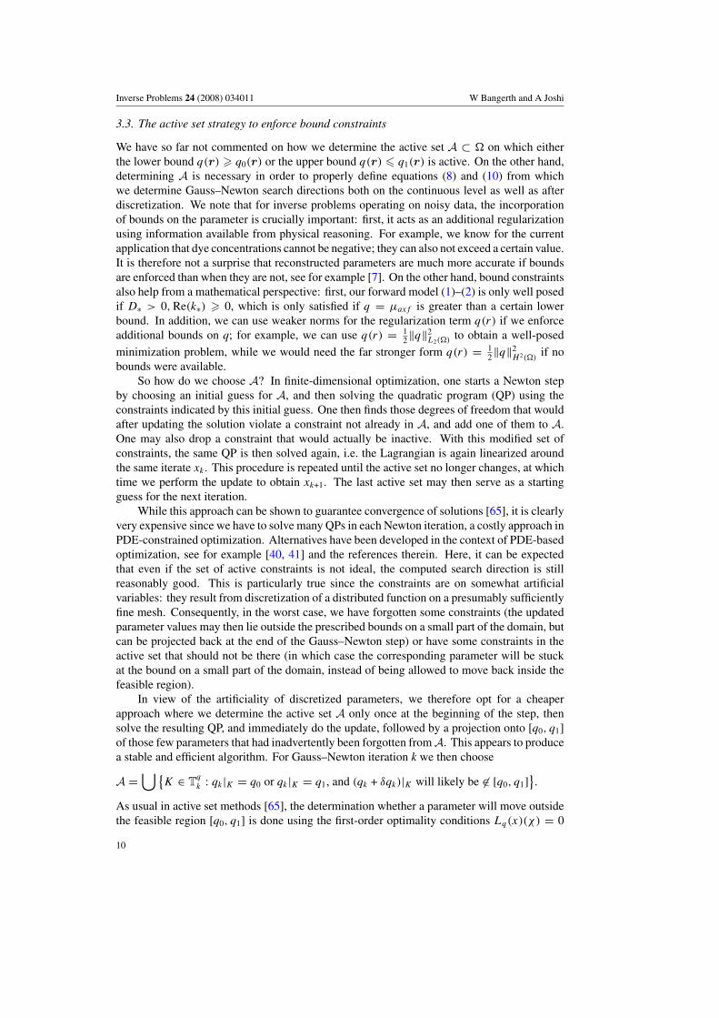
Finally, the left panel of figure 5 shows some statistics of computations. The curves showhow refinement between iterations increases the total number of degrees of freedom frominitially some 104 per experiment to around 2.5 × 105 per experiment. At the same time, thenumber of parameters discretized on T

q increases from 288 to 2787. In this example, only anegligible number of unknowns in qk are constrained by bounds.

3 The diffusion length scale for light in the chosen medium is around 2 mm. Any information on scales smallerthan this can therefore not be recovered within the framework of the diffusion approximation (1)–(2). Our mesh isconsequently able to resolve all resolvable features.

16

Inverse Problems 24 (2008) 034011 W Bangerth and A Joshi

Figure 4. Left column: volume rendering of reconstructed parameters qk at the end of iterations.Right column: those cells where qk(r) � 50% maxr′∈� qk(r

′) are shown as blocks, whereas theactual location and size of the targets are drawn as spheres. In addition, the mesh on three cutplanes through the domain is shown. Top row: single target reconstruction. Bottom row: threetarget reconstructions.

4.2. Three target reconstruction

In a second experiment, we attempt to reconstruct with synthetic data generated from threeclosely spaced targets with centers at r1 = (3, 2, 6), r2 = (4, 5, 6), r3 = (7, 3, 6) anddiameters of again 5 mm. As for the first example, the bottom row of figure 3 shows asequence of meshes T

q

k , whereas figure 4 shows a closer look at the reconstructed parameter.Again, the location of the reconstructed targets is mostly correct, but the two targets closesttogether are blurred—a well-known phenomenon in diffusive imaging.

The right panel of figure 5 shows statistics about this computation. Most noteworthy isthat in this example the number of constrained parameter degrees of freedom is much moresignificant than in the first one: after the first few iterations, between 40% and 60% of allparameters are constrained. As mentioned in section 3.2, the bounds do not only help tostabilize the problem, but also make the solution of the Schur complement simpler sinceconstrained degrees of freedom are eliminated from the system.

17

Inverse Problems 24 (2008) 034011 W Bangerth and A Joshi

10

100

1000

10000

100000

1e+06

1e+07

1e+08

2 4 6 8 10 12Gauss-Newton iteration

Single target reconstruction

Size of KKT systemNumber of parameters

Number of constrained parameters

(a)

10

100

1000

10000

100000

1e+06

1e+07

1e+08

5 10 15 20 25 30Gauss-Newton iteration

Three target reconstruction

Size of KKT systemNumber of parameters

Number of constrained parameters

(b)

Figure 5. Total number of unknowns accumulated over all experiments (i.e. the size of the KKTmatrix (10)), number of unknowns in the parameter mesh T

q

k , and number of parameters that areactively constrained by bounds q0 � qk � q1 for the single target reconstruction (left) and threetarget reconstruction experiments (right).

1e-16

1e-15

1e-14

1e-13

1e-12

1e-11

1e-10

5 10 15 20 25 30

Gauss-Newton iteration

Data misfitRegularization term

Regularization parameter

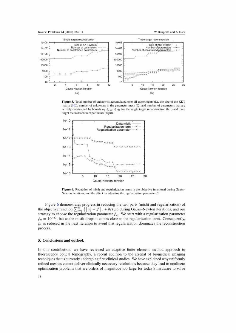
Figure 6. Reduction of misfit and regularization terms in the objective functional during Gauss–Newton iterations, and the effect on adjusting the regularization parameter β.

Figure 6 demonstrates progress in reducing the two parts (misfit and regularization) ofthe objective function

∑Wi=1

12

∥∥uik − zi

∥∥�

+ βr(qk) during Gauss–Newton iterations, and ourstrategy to choose the regularization parameter βk . We start with a regularization parameterβ0 = 10−12, but as the misfit drops it comes close to the regularization term. Consequently,βk is reduced in the next iteration to avoid that regularization dominates the reconstructionprocess.

5. Conclusions and outlook

In this contribution, we have reviewed an adaptive finite element method approach tofluorescence optical tomography, a recent addition to the arsenal of biomedical imagingtechniques that is currently undergoing first clinical studies. We have explained why uniformlyrefined meshes cannot deliver clinically necessary resolutions because they lead to nonlinearoptimization problems that are orders of magnitude too large for today’s hardware to solve

18

Inverse Problems 24 (2008) 034011 W Bangerth and A Joshi

within clinically acceptable time scales. Our solution to this problem was the introduction ofadaptively refined meshes. They not only are able to focus numerical effort to regions in thedomain where high resolution is actually necessary, but also regularize the inverse problem andin particular make the initial Gauss–Newton iterations extremely cheap since we can computeon coarse meshes while we are still far away from the solution.

Using a sequence of meshes that change adaptively as iterations proceed requiresadjusting some of the techniques traditionally known from optimization methods since thedimensionality of the problem changes between iterations, and continuous and discrete normsare no longer equivalent under adaptive mesh refinement. For example, nonlinear iterationsand mesh refinement algorithms have to be interconnected to achieve efficient methods, andactive set strategies for inequality constraints need to be modified for locally refined meshes.

We have therefore presented a comprehensive framework for the solution of opticaltomography problems with adaptive finite element methods. The workings and efficiency ofthis framework have been demonstrated with two practically relevant numerical examples.

However, although we are able to efficiently solve this inverse problem to practicallynecessary resolution, it would be a mistake to believe that there is no need to improve it. Inparticular, we believe that further progress is necessary in the following areas:

• Linear solvers: because the Schur complement S defined in (14) is only known throughits action on vectors, it is complicated to derive preconditioners for the reduced system(15) in which our solvers spend 75% of the compute time on fine meshes. It is thereforeimportant to think about viable ways to precondition this equation. One approach wouldbe to use BFGS or LM-BFGS approximations of S−1 (see [65]) as used in [17]. However,they would have to be integrated with adaptivity since they expect the parameter space toremain fixed.

• Multigrid: another approach is to use multilevel algorithms for the Schur complement orthe whole KKT system. Methods in this direction have already been explored in [2, 5,21, 54].

• Systematic characterization of results: for practical usability, numerical methods do notonly have to work in simple situations like the ones shown in section 4, but also inthe presence of significant background heterogeneity, unknown or large noise levels,systematic measurement bias and other practical constraints. Systematic testing ofreconstructions for statistically sampled scenarios with objective assessment of imagequality (OAIQ) methods [70] will be necessary to achieve clinical use.

• Optimal experimental design techniques should enable us to improve our experimentalsetups to make them more sensitive to the quantities we intend to recover. However, theylead to non-convex optimization problems with the inverse problem as a subproblem, andtherefore to computationally extremely complex problems.

Despite our belief that the algorithms we have presented are powerful tools in makingfluorescence optical tomography a valuable imaging tool of the future, above list indicates thatmuch research is left in this and related problems.

Acknowledgment

Part of this work was supported by NSF grant DMS-0604778.

19

Inverse Problems 24 (2008) 034011 W Bangerth and A Joshi

References

[1] Abdoulaev G S, Ren K and Hielscher A H 2005 Optical tomography as a PDE-constrained optimization problemInverse Problems 21 1507–30

[2] Adavani S S and Biros G 2007 Multigrid algorithms for inverse problems with linear parabolic PDE constraints,submitted

[3] Ainsworth M and Oden J T 2000 A Posteriori Error Estimation in Finite Element Analysis (New York: Wiley)[4] Arridge S R 1999 Optical tomography in medical imaging Inverse Problems 15 R41–93[5] Ascher U M and Haber E 2003 A multigrid method for distributed parameter estimation problems Electron

Trans. Numer. Anal. 15 1–12[6] Bangerth W 2002 Adaptive finite element methods for the identification of distributed parameters in partial

differential equations PhD Thesis University of Heidelberg[7] Bangerth W 2008 A framework for the adaptive finite element solution of large inverse problems SIAM J. Sci.

Comput. at press[8] Bangerth W, Hartmann R and Kanschat G 2007 deal.II—a general purpose object oriented finite element library

ACM Trans. Math. Softw. 33 1–24/27[9] Bangerth W, Hartmann R and Kanschat G 2008 deal.II differential equations analysis library Technical Reference

http://www.dealii.org/[10] Bangerth W and Rannacher R 2003 Adaptive Finite Element Methods for Differential Equations (Basle:

Birkhauser)[11] Banks H T and Kunisch K 1989 Estimation Techniques for Distributed Parameter Systems (Basel: Birkhauser)[12] Becker R 2001 Adaptive finite elements for optimal control problems Habilitation Thesis University of

Heidelberg[13] Becker R, Kapp H and Rannacher R 2000 Adaptive finite element methods for optimal control of partial

differential equations: basic concept SIAM J. Control Optim. 39 113–32[14] Becker R and Vexler B 2003 A posteriori error estimation for finite element discretization of parameter

identification problems Numer. Math. 96 435–59[15] Ben Ameur H, Chavent G and Jaffre J 2002 Refinement and coarsening indicators for adaptive parametrization:

application to the estimation of hydraulic transmissivities Inverse Problems 18 775–94[16] Biros G and Ghattas O 2003 Inexactness issues in the Lagrange-Newton-Krylov-Schur method for PDE-

constrained optimization Large-Scale PDE-Constrained Optimization (Lecture Notes in ComputationalScience and Engineering vol 30) ed L T Biegler, O Ghattas, M Heinkenschloss and B van BloemenWaanders (Berlin: Springer) pp 93–114

[17] Biros G and Ghattas O 2005 Parallel Lagrange-Newton-Krylov-Schur methods for PDE-constrainedoptimization: Part I. The Krylov-Schur solver SIAM J. Sci. Comput. 27 687–713

[18] Biros G and Ghattas O 2005 Parallel Lagrange-Newton-Krylov-Schur methods for PDE-constrainedoptimization: Part II. The Lagrange-Newton solver and its application to optimal control of steady viscousflow SIAM J. Sci. Comput. 27 714–39

[19] Borcea L and Druskin V 2002 Optimal finite difference grids for direct and inverse Sturm Liouville problemsInverse Problems 18 979–1001

[20] Borcea L, Druskin V and Knizhnerman L 2005 On the continuum limit of a discrete inverse spectral problemon optimal finite difference grids Comm. Pure. Appl. Math. 58 1231–79

[21] Borzı A, Kunisch K and Kwak D Y 2003 Accuracy and convergence properties of the finite difference multigridsolution of an optimal control problem SIAM J. Control Optim. 41 1477–97

[22] Carey G F 1997 Computational Grids: Generation, Adaptation and Solution Strategies (London: Taylor andFrancis)

[23] Chance B et al 1988 Comparison of time-resolved and unresolved measurements of deoxyheamoglobin in brainProc. Natl Acad. Sci. 85 4791–975

[24] Chandrasekhar S 1960 Radiative Transfer (New York: Dover)[25] Chernomordik V, Hattery D, Gannot I and Gandjbakhche A H 1999 Inverse method 3-D reconstruction

of localized in vivo fluorescence-application to Sjøgren syndrome IEEE J. Sel. Top. Quantum Electron.54 930–5

[26] Collis S S, Ghayour K, Heinkenschloss M, Ulbrich M and Ulbrich S 2002 Optimal control of unsteady viscousflows Int. J. Numer. Methods Fluids 40 1401–29

[27] Engl H W, Hanke M and Neubauer A 1996 Regularization of Inverse Problems (Dordrecht: Kluwer)[28] Eppstein M J, Hawrysz D J, Godavarty A and Sevick-Muraca E M 2002 Three dimensional near infrared

fluorescence tomography with Bayesian methodologies for image reconstruction from sparse and noisy datasets Proc. Natl. Acad. Sci. 99 9619–24

20

Inverse Problems 24 (2008) 034011 W Bangerth and A Joshi

[29] Gago J P de S R, Kelly D W, Zienkiewicz O C and Babuška I 1983 A posteriori error analysis andadaptive processes in the finite element method: II. Adaptive mesh refinement Int. J. Numer. Methods Eng.19 1621–56

[30] Godavarty A, Eppstein M J, Zhang C, Theru S, Thompson A B, Gurfinkel M and Sevick-Muraca E M 2003Fluorescence-enhanced optical imaging in large tissue volumes using a gain-modulated ICCD camera Phys.Med. Biol. 48 1701–20

[31] Graves E E, Ripoll J, Weissleder R and Ntziachristos V 2003 A submillimeter resolution fluorescence molecularimaging system for small animal imaging Med. Phys. 30 901–11

[32] Guven M, Yazici B, Intes X and Chance B 2003 An adaptive multigrid algorithm for region of interest diffuseoptical tomography Proc. Int. Conf. on Image Processing vol 2 pp 823–6

[33] Guven M, Yazici B, Kwon K, Giladi E and Intes X 2007 Effect of discretization error and adaptive meshgeneration in diffuse optical absorption imaging: I Inverse Problems 23 1115–34

[34] Guven M, Yazici B, Kwon K, Giladi E and Intes X 2007 Effect of discretization error and adaptive meshgeneration in diffuse optical absorption imaging: II Inverse Problems 23 1124–60

[35] Haber E, Heldmann S and Ascher U 2007 Adaptive finite volume methods for distributed non-smooth parameteridentification Inverse Problems 23 1659–76

[36] Hebden J C, Gibson A, Austin T, Yusof R M, Everdell N, Delpy D T, Arridge S R, Meek J H and Wyatt J S2004 Imaging changes in blood volume and oxygenation in the newborn infant brain using three-dimensionaloptical tomography Phys. Med. Biol. 49 1117–30

[37] Hebden J C, Gibson A, Yusof R M, Everdell N, Hillman E M C, Delpy D T, Arridge S R, Austin T,Meek J H and Wyatt J S 2002 Three-dimensional optical tomography of the premature infant brain Phys.Med. Biol. 47 4155–66

[38] Heinkenschloss M 1991 Gauss-Newton methods for infinite dimensional least squares problems with normconstraints PhD Thesis University of Trier, Germany

[39] Heinkenschloss M and Vicente L 1999 An interface between optimization and application for the numericalsolution of optimal control problems ACM Trans. Math. Softw. 25 157–90

[40] Hintermuller M and Hinze M A SQP-semi-smooth Newton-type algorithm applied to control if the instantionaryNavier-Stokes system subject to control constraints SIAM J. Optim. at press

[41] Hintermuller M, Ito K and Kunisch K 2002 The primal-dual active set strategy as a semismooth newton methodSIAM J. Optim. 13 865–88

[42] Hoppe R H W, Iliash Y, Iyyunni C and Sweilam N H 2006 A posteriori error estimates for adaptive finiteelement discretizations of boundary control problems J. Numer. Anal. 14 57–82

[43] Hull E L, Nichols M G and Foster T H 1998 Localization of luminescent inhomogeneities in turbid media withspatially resolved measurements of CW diffuse luminescence emittance Appl. Opt. 37 2755–65

[44] Ito K and Kunisch K 1992 On the choice of the regularization parameter in nonlinear inverse problemsSIAM J. Optim. 2 376–404

[45] Johnson C R 1997 Computational and numerical methods for bioelectric field problems Crit. Rev. Biomed. Eng.25 1–81

[46] Joshi A, Bangerth W, Hwang K, Rasmussen J and Sevick-Muraca E M 2006 Fully adaptive FEM basedfluorescence optical tomography from time-dependent measurements with area illumination and detectionMed. Phys. 33 1299–310

[47] Joshi A, Bangerth W, Hwang K, Rasmussen J and Sevick-Muraca E M 2006 Plane wave fluorescence tomographywith adaptive finite elements Opt. Lett. 31 193–5

[48] Joshi A, Bangerth W, Hwang K, Rasmussen J C and Sevick-Muraca E M 2006 Fully adaptive FEM basedfluorescence optical tomography from time-dependent measurements with area illumination and detectionMed. Phys. 33 1299–310

[49] Joshi A, Bangerth W and Sevick-Muraca E M 2004 Adaptive finite element modeling of optical fluorescence-enhanced tomography Opt. Express 12 5402–17

[50] Joshi A, Bangerth W and Sevick-Muraca E M 2006 Non-contact fluorescence optical tomography with scanningpatterned illumination Opt. Express 14 6516–34

[51] Joshi A, Bangerth W, Sharma R, Rasmussen J, Wang W and Sevick-Muraca E M 2007 Molecular tomographicimaging of lymph nodes with NIR fluorescence Proc. 2007 IEEE International Symposium on BiomedicalImaging pp 564–7

[52] Kaipio J and Somersalo E 2006 Statistical and Computational Inverse Problems (Berlin: Springer)[53] Kaipio J P, Kohlemainen V, Somersalo E and Vauhkonen M 2000 Statistical inversion and Monte Carlo sampling

methods in electrical impedance tomography Inverse Problems 16 1487–522[54] Kaltenbacher B 2001 On the regularization properties of a full multigrid method for ill-posed problems Inverse

Problems 17 767–88

21

Inverse Problems 24 (2008) 034011 W Bangerth and A Joshi

[55] Kunisch K, Liu W and Yan N 2002 A posteriori error estimators for a model parameter estimation problemProc. ENUMATH 2001 Conf.

[56] Li R, Liu W, Ma H and Tang T 2002 Adaptive finite element approximation for distributed elliptic optimalcontrol problems SIAM J. Control Optim. 41 1321–49

[57] Li X D, Chance B and Yodh A G 1998 Fluorescent heterogeneities in turbid media: limits for detection,characterization, and comparison with absorption Appl. Opt. 37 6833–44

[58] Li X D, O’Leary M A, Boas D A, Chance B and Yodh A G 1996 Fluorescent diffuse photon density waves inhomogenous and heterogeneous turbid media: analytic solutions and applications Appl. Opt. 35 3746–58

[59] Meidner D and Vexler B 2007 Adaptive space-time finite element methods for parabolic optimization problemsSIAM J. Control Optim. 46 116–42

[60] Milstein A B, Kennedy M D, Low P S, Bouman C A and Webb K J 2005 Statistical approach for detection andlocalization of a fluorescing mouse tumor in intralipid Appl. Opt. 44 2300

[61] Milstein A B, Oh S, Webb K J, Bouman C A, Zhang Q, Boas D and Milane R P 2003 Fluorescence opticaldiffusion tomography Appl. Opt. 42 3061–94

[62] Molinari M, Blott B H, Cox S J and Daniell G J 2002 Optimal imaging with adaptive mesh refinement inelectrical impedence tomography Physiol. Meas. 23 121–8

[63] Molinari M, Cox S J, Blott B H and Daniell G J 2001 Adaptive mesh refinement techniques for electricalimpedence tomography Physiol. Meas. 22 91–6

[64] Mosegaard K and Tarantola A 2002 Probabilistic approach to inverse problems International Handbook ofEarthquake and Engineering Seismology (Part A) (New York: Academic) pp 237–65

[65] Nocedal J and Wright S J 1999 Numerical Optimization (Springer Series in Operations Research) (New York:Springer)

[66] O’Leary D 2001 Near-optimal parameters for Tikhonov and other regularization schemes SIAM J. Sci. Comput.23 1161–71

[67] O’Leary M A, Boas D A, Chance B and Yodh A G 1994 Reradiation and imaging of diffuse photon densitywaves using fluorescent inhomogeneities J. Lumin. 60 281–6

[68] O’Leary M A, Boas D A, Chance B and Yodh A G 1996 Fluorescence lifetime imaging in turbid media Opt.Lett. 20 426–8

[69] Roy R, Thompson A B, Godavarty A and Sevick-Muraca E M 2005 Tomographic fluorescence imaging in tissuephantoms: a novel reconstruction algorithm and imaging geometry IEEE Trans. Med. Imaging 24 137–54

[70] Sahu A, Joshi A, Kupinsky M and Sevick-Muraca E M 2006 Assessment of a fluorescence enhanced opticalimaging system using the Hotelling observer Opt. Express 14 7642–60

[71] Scherzer O, Engl H W and Kunisch K 1993 Optimal a-posteriori parameter choice for Tikhonov regularizationfor solving nonlinear ill-posed problems SIAM J. Numer. Anal. 30 1796–838

[72] Schotland J C 1997 Continuous wave diffusion imaging J. Opt. Soc. Am. A 14 275–9[73] Schulz R B, Ripoll J and Ntziachristos V 2004 Experimental fluorescence tomography of tissues with noncontact

measurements IEEE Trans. Med. Imaging 23 492–500[74] Sevick-Muraca E M and Burch C L 1994 The origin of phosphorescent and fluorescent signals in tissues Opt.

Lett. 19 1928–30[75] Sevick-Muraca E M, Kuwana E, Godavarty A, Houston J P, Thompson A B and Roy R 2003 Near infrared

fluorescence imaging and spectroscopy in random media and tissues Biomedical Photonics Handbook (BocaRaton, FL: CRC Press) chapter 33

[76] Sevick-Muraca E M, Lopez G, Troy T L, Reynolds J S and Hutchinson C L 1997 Fluorescence and absorptioncontrast mechanisms for biomedical optical imaging using frequency-domain techniques Photochem.Photobiol. 66 55–64

[77] Srinivasan S, Pogue B W, Jiang S, Dehghani H, Kogel C, Soho S, Gibson J J, Tosteson T D, Poplack S Pand Paulsen K D 2003 Interpreting hemoglobin and water concentration, oxygen saturation, and scatteringmeasured in vivo by near-infrared breast tomography Proc. Natl Acad. Sci. 100 12349–54

[78] Tarantola A 2004 Inverse Problem Theory and Methods for Model Parameter Estimation (Philadelphia: SIAM)[79] Ulbrich M, Ulbrich S and Heinkenschloss M 1999 Global convergence of trust-region interior-point

algorithms for infinite-dimensional nonconvex minimization subject to pointwise bounds SIAM J. ControlOptim. 37 731–64

[80] Vexler B and Wollner W 2008 Adaptive finite elements for elliptic optimization problems with control constraintsSIAM J. Control Optim. 47 509–34

[81] Wu J, Wang Y, Perleman L, Itzkan I, Desai R R and Feld M S 1995 Time resolved multichannel imaging offluorescent objects embedded in turbid media Opt. Lett. 20 489–91

22