Numerical Analysis ‘Project s. June 1990Manuscript NA-90-07 . . .

Adaptive Lanczos Methods

for

Recursive Condition Estimation

bY

William R. FerngGene H. Golub

Robert J. Plemmons

Numerical Analysis ProjectComputer Science Department

Stanford UniversityStanford, California 94305

Adaptive Lanczos Methodsfor

Recursive Condition Estimation

William R. Ferng* Gene H. GolubtRobert J. Plemmons $

May 31, 1990

AbstractEstimates for the condition number of a matrix are useful in many areas of scientific

computing, including: recursive least squares computations, optimization, eigenanal-ysis, and general nonlinear problems solved by linearization techniques where matrixmodification techniques are used. The purpose of this paper is to propose an adaptive~anczos gstimator scheme, which we call ale, for tracking the condition number of themodified matrix over time. Applications to recursive least squares (RLS) computationsusing the covariance method with sliding data windows are considered. uk is fast forrelatively small n - parameter problems arising in RLS methods in control and signalprocessing, and is adaptive over time, i.e., estimates at time t are used to produceestimates at time t + 1. Comparisons are made with other adaptive and non-adaptivecondition estimators for recursive least squares problems. Numerical experiments arereported indicating that ale yields a very accurate recursive condition estimator.

Subject Classifications: AMS( MOS): 15A18, 65F10, 65F20, 65F35Key Words: adaptive methods, conditiod estimation, control, downdating, eigenvalues,Lanczos methods, matrix modifications, recursive least squares, signal processing, singularvalues, updatingRunning Title: Adaptive Lanczos Estimator

*Department of Mathematics, NC State University, Raleigh, NC 276958205. Research supported by theUS Air Force under grant no. AFOSR88-0285.

tDepartment of Computer Science, Stanford University, Stanford, CA 94305. Research supported by theUS Army under grant no. DAAL03-90-G-105.

t Department of Mathematics and Computer Science, Wake Forest University, P.O. Box 7311, Winston-Salem, N.C. 27109. Research supported by the US Air Force under grant no. AFOSR-88-0285.

1

1 IntroductionRepeated estimates for the condition number of a matrix are useful assessing the accuracyand stability of algorithms employed in many application areas of scientific computing,including: optimization, least squares computations, eigenanalysis, and general nonlinearproblems solved by linearization techniques [3], [20], [2l], [35]. Our purpose in this paperis to propose an adaptive ~anczos estimator scheme, which we call ale, for tracking thecondition number of the modified matrix over time. The key computations involve theadaptive estimation of extreme singular values and vectors for a triangular factor L. Wedevelop adaptive Lanczos schemes for estimating extreme singular values and vectors of Lfor each recursive modification. Approximations to the secular equations for the modifiedmatrix are used to obtain good starting vectors for the Lanczos schemes. Applications torecursive least squares (RLS) computations using the covariance method with sliding datawindows in control and signal processing are considered. The computations are adaptiveover time in the sense that estimates at time t are used to obtain estimates at time t + 1.

An alternative adaptive condition estimation scheme, called ace and based on opti-mization principles, has been suggested by Pierce and Plemmons [31], and applied tocomputations in adaptive control and signal processing in [32], [33]. A non-adaptive in-cremental condition estimation scheme, called ice, has been suggested by Bischof [5], andapplied to computations in signal processing in [S] in a different context. It might be help

- ful to clarify the use of the words ‘incremental’ versus ‘adaptive’. ‘Incremental’ ice obtainscondition estimates of a triangular factor that grows, whereas ‘adaptive’ ale and ace main-tain condition estimates when information is added/extracted from an already existingfactorization. Comparisons of ale with ace and ice on recursive least squares applicationsare included in this paper. We begin by reviewing least squares computations.

1.1 Least SquaresThe linear lead squares problem can be posed as follows: Given a real m x n matrix Xwith full column rank n and a real m-vector 8, find the n-vector w that solves

min 118 - Xwlla,where ]I l 112 denotes the usual Euclidean norm. The solution to (1) is given by

w = (XTX)-‘XT&

0)

(2)If R denotes the upper triangular ChoZesEy factor of the cross product matrix XTX, i.e.,RTR = XTX, then w can be obtained by solving the triangular systems RTv = XTs,followed by Rw = v, where v is an intermediate vector. However, in many applicationswhere accuracy and stability are important [20], R is computed directly from X by asequence of orthogonal transformations; that is

QX R= [ 10 ’ QTQ = I.

2

Then setting

Qs = [ 1i , c an n-vector, (4)w is computed by solving the upper triangular system Rw = c. In addition, the matrix

P E (X’X)-’ (5)is called the covariance matrix for (1). It measures the expected errors in the least squaresvector w. Its inverse

P-’ = XTX, (6)often called the normal equations matrix [2O], is known as the information matrix for (1)in the signal processing literature [l], [4], [2l]. It measures the information content in theexperiment leading to (1).

1.2 Recursive Least SquaresIn recursive Zeast squares (RLS) it is required to recalculate w when observations (i.e.,equations) are successively added to, or deleted from, the problem (1). For example, inmany applications information arrives continuously and must be incorporated into thesolution w. This is called updating. It is sometimes important to delete old observations

- and have their effect excised from 20. This is called downdating and is associated with a3ding data window. Alternatively, an exponential forgetting factor A, with 0 < A ,< 1 (see,e.g., [21]), may be incorporated into the updating computations to exponentially decay theeffect of the old data over time. The use of A is associated with an exponentially-weighteddata window [3], [2l]. In this paper we will consider the standard updating and downdatingmethods, which can be associated with applications to sliding window methods in RLS.For details on implementations of these sliding window methods see [2], [4], [7], [s], [12],or [33].

There are two main approaches to solving recursive least squares problems; the in-fomnation matrix method based upon modifying P-l = XTX and the covariance matrixmethod based upon modifying P [l], [4], [21]. Instead of modifying P-l or P directly, itis generally preferable for stability and cost reasons to modify their Cholesky factors [4].We will concentrate on the covariance matrix method in this paper. Applications of ale totracking the conditioning of P-l = XTX in the information matrix method are similar.

RLS computations arising in adaptive control and signal processing can be describedas follows. We assume that the arriving data is prewindowed (e.g., [l], [3]) so that thediscrete time index begins at 1. For k: 2 1, we let z(h) denote the arriving column datavector of dimension n at time Ic. At time m 2 n, the data matrix X defined in (1) isdenoted by X(m). Consequently, the covariance matrix P defined in (5) can be written as

-1

P z P(m) = (X(m)TX(m))-’ = &(k)z(k)T 1 . (7)k=l

3

To initialize the RLS process, P, or P-l, is often set to a scalar multiple of the identitymatrix SI.

From (7) it follows that if the data vectors z(k) do not go to zero, then the eigenvaluesof the covariance matrix P decrease monotonically. A common procedure, e.g., [l], [3],[21], is to monitor the smallest singular value, Xmin (P(m)), and reset P(m + 1) to SI whenh@‘(m)) falls b 1e ow some tolerance factor. This process is called covariance TeJetting,or reinitialization (e.g., [35] p. 62). Alternatively, a time window can be introduced todownweight the influence of past observation or errors, and accordingly, prevent a possiblerapid decrease in X,,,i,,( P( m)).

There are two types of time windows: sliding windows and exponentially-weighted win-dows, the latter of which is a special case of our work and thus will not be discussed further.When a sliding window approach is used, then a fixed window length I > n is chosen. Foreach time m in the recursive process, the problem is updated by adding the (m + l)8tobservation and the effect of the old (m - 2 + I>,’ observation is completely removed bydowndating (e.g., [2]). This sliding window approach approximately doubles the compu-tational complexity of the basic updating process with exponentially-weighted windows,but is well-known to possess favorable convergence or signal tracking characteristics [3],PI7 M

RLS algorithms based upon modifying the Cholesky factor L c ReT of P = (XTX)-lare reviewed in Section 2. Adaptive Lanczos based condition estimation schemes for trian-

- gular factor updating and downdating are developed in Section 3. Reports on numericaltests with some ill-conditioned data and some actual signal processing data in RLS com-putations, along with some final comments, are given in Section 4.

2 RLS Sliding Window ComputationsWe now consider the sliding window recursive least squares (RLS) computations and pro-ceed to simplify the notation. Updating computations are considered first.

At time m+l, weset y = z(m + 1). Now, consider the least squares problem (1) and,without loss of generality, assume that the additional data vector y and scalar 0 for theequation

yTw = y1 w1 + l l l + ynw, ⌧ u

are appended to X and s forming

z=[;], a=[;]. (8)One now seeks to solve the modified problem

min ]]Z - XG]]~ (9)for the updated least squares estimate vector G. This process is then repeated at eachrecursive time step.

4

The process of modifying least squares computations by updating the covariance matrixP has been used in control and signal processing for some time in the context of linearsequential filtering [l], [4], [2l], [29]. One begins with estimates for P = RelRmT (whereR is the Cholesky factor of XTX) and w, and updates R-l to R-’ and w to 6 at eachrecursive time step. Recently Pan and Plemmons [30] have described a parallel scheme forthese computations.

Observe first that with X given in (8), p-l is given by

F-l = XTF = xTx + YYT = p-l + Y$/T.

Consequently, by the Sherman-Morrison formula (see, e.g., [2O]),

&p-- l1+ y’Py

PyyTP.

The updated w is given by

By substituting (8) and (10) into (11) and using the representation (2) for w, there results- the following basic formula for the update:

G = w + Fy(u - yTw)* 02)

The vectorkdy (13)

is often called the Kalman gain vector (see, e.g., [l], [4], [Zl]). It weights the predictedresidual 0 - yTw. Updating schemes based upon applying (10) and (12) directly are calledConventional RLS Algorithm3 [1], [3], [4], [21]. Such approaches can lead to numericaldifficulties, e.g., loss of symmetry and/or loss of positive definiteness in P. Better numericalresults can be expected when the Cholesky factor L E ReT of P = (XTX)-l, rather thanP itself, is updated [4], and we adopt that premise in this paper.

Computational schemes for updating the Cholesky factor R typically employ the ap-plication of orthogonal plane rotations Q; to zero the update vector yT. In particular,orthogonal plane rotations Q;,n+r, rotating the jth row into the (n + l)8t row, are formedfor the reduction

Qn..,rQ~,n+~[ ;] = [f],

so that the updated matrix fi is upper triangular.Covariance matrix downdating is considered next. Many of the downdating concepts

are similar to those for covariance matrix updating, and will only be summarized for thesake of brevity. We assume that, for stability purposes, the updating step is performed

5

before downdatinglsee, e.g., [SO]). Thus b fe ore a downdating step we assume that X hasbeen modified to X and the observation vector s to Z, by updating the Cholesky factorL s R-l of P = (X’X)-l to 2 and the least squares estimate w to 6.3. For simplicity ofnotation, we replace [X, s, L, w] with the updated [X, Z, Z, ~1 in some of our discussionof downdating to follow.

The downdating computation in RLS with sliding data windows can be described inthe following way. Here the purpose is to remove the effect of an observation on the currentleast squares vector w; that is, to remove a row zT from the observation matrix X and ascalar 7 from the observation vector 5, corresponding to the observation

ITW = qq + l l l + %,W, ⌧ 7).

Assume that zT is the first row of X, so that X and s are related to the downdated X and

qq, -I=[;].In this case the modified covariance matrix satisfies

p-1 = Fx^ = XTX + yyT - %rT = P-l + yyT - rrT,

- where y is the update vector and z the downdate vector. If R is the updated Choleskyfactor of XTX, it follows that the modified Cholesky factor fi satisfies RTff = RTR - %rT.Assuming that X retains full column rank, the covariance downdating problem is now touse the updated inverse Cholesky factor L G R-l of the updated P = (XTX)-l to computethe downdated inverse factor 2 and the downdated least squares vector $. But now theorthogonal rotation schemes do not apply directly, due to the negative sign of zzT. A com-putationally efficient scheme based upon the use of hyperbolic transformations H; ratherthan orthogonal trigonometric plane rotations &i can used to compute the downdatedfactor. For brevity, we refer the reader to the second edition of [20], Section 12.6.4, for adetailed discussion of the use hyperbolic transformations H; for downdating. We commentthat, for stability reasons, these transformations should be implemented as described byGolub [16] (see also [2]). -

The following RLS sliding window scheme for modifying the covariance matrix P byupdating RBT to ii-T followed by downdating to R-T and for computing the correspondingmodified least squares estimate vector 6 was given in [30] (see also Morf and Kailath [29]).Here we write P = LTL , where L E ReT.

Algorithm 1 (RLS by the Sliding Window Covariance Method) . Given the CUT-rent n-dimensional leaz?t squares eArnate vector 20, the current lower triangular factorL G RmT of P = (X’X)-I, the observation yT,[ Io being added, and the the observation

ZT[ d

, q being removed, the algorithm computea the modified factor 2 E kT of p and themodi ed least squares estimate vector 12.

6

1.

2.

3.

4*5.

6.

7.

8.

Form the mat& vector product a = Ly.

Choose orthogonal plane rotations G;,,+l, rotating the ith component into the (n+I)8tcomponent, to form

by reducing -a to 0 from the top down, and form

(15)

(16)

preserving the lower triangular form of L in z.

Compute1-

6 = w - -u(a - yTw).6 (17)

Replace [L, w] c [E, iE].

Form the mat& vector product b = Lz.Choose hyperbolic rotation3 H;,,+I, rotating the ith component into the (n+ l)8t com-ponent, to form

by reducing b to 0 from the top down, and form

(19)

preserving the lower triangular form of L in z.

Computec=‘ui- 1

yv(r] - rTw). (20)

Replace [L, w] + [Z, $1, input the new observation [yT, o] to be added, let [zT,q]denote the old observatton to be removed and return to Step 1.

Some comments about the algorithm are in order. First, the rotation parameters in(15) and (18) are computed successively using the components of the vectors a and b. Itfollows from [SO], that u in the update step and v in the downdate step are scaled formsof the Kalman gain vectors associated with updating and downdating. The algorithmrequires up to 5n2 + O(n) multiplications per time step. The 5n2 term comes entirely fromupdating and downdating L. No triangular solves are involved.

7

Our purpose now is to develop an adaptive scheme for monitoring the spectral conditionnumber of L, and accordingly the covariance matrix P, after each recursive time step. Anadaptive Lanczos based condition estimation scheme, which we call ale, for monitoringcondition numbers of the covariance matrices over time by tracking the extreme singularvalues and singular vectors of the Cholesky factors is described in the next section.

3 ALE: Adaptive Lanceos EstimatorOur purpose is to describe schemes for adaptively monitoring the extreme singular valuesin RLS updating methods associated with updating and downdating.

The Lanczos method [19], [25] can be used to reduce a nonsymmetric matrix A to abidiagonal matrix, that is, if A E Rnxn, the Lanczos method computes orthogonal matricesU and V, such that

UTAV = B (21)where B is a lower bidiagonal matrix. It follows that A and B have the same singularvalues.

It is well known that the information about the extreme singular values trends toemerge long before the bidiagonalization process is complete [US]. In our application, weare only interested in estimating the extreme singular values. We will employ this fastconvergence characteristic of the Lanczos method for only a few iterations to approximatethe extreme singular values, hence the condition number.

Our purpose is to monitor the spectral condition number of Cholesky factor during lowrank modifications; in particular, after rank-one updating and downdating. We then applythe Lanczos method to an n x n lower triangular Cholesky matrix L in Algorithm 1 for kiterations, computing orthonormal vectors uj and vj, such that

U(k)TLV(k) = B(k) (22)

where V(k) = [ui, u2,. . . , uk], V(k) = [vi, v2,. . . , vk], and B(k) is a k x k lower bidiagonalmatrix with the following form

(23)

The maximal singular value of L is approximated by the maximal singular value of B(k),that is, amas x am&B(k)), c.f., [19]. The minimal singular value of L can be ap-proximated in a similar way. The following algorithm describes the scheme for estimating

Algorithm 2 (Lanczos Method) . Given a lower triangular matrix L E Rnxn, and anarbitrary vector 211, Ilu& = 1, the algorithm computes orthonormal vectors vj and uj andthe entries of the bidiagonal matrix B(k), such that amax e amax(B(k)).

1. Input [L,u,].

2. Compute cyl = llLTuJ2, and set v1 = $L%l.

3. Forj=1,2 ,..., (k-l)(a) Compute pj = IILvj - ajujllz, and set uj+l = $(Lvj - ajuj),t

(b) Compute aj+l = IlLT uj+l - pivjll2, and set vj+l = &(LTuj+l- Pjvj),

end for

4. Construct lower bidiagonal matrix B(k), -and compute amax(B

Note that the Lanczos method is applied for k steps ( k - 1 iterations in the for loop ),and this k may be much smaller than the problem size n. For example, in our numericalexperiments, we let k = 2, and the algorithm generates a 2 x 2 lower bidiagonal matrixwhose maximal singular value can be computed directly by a quadratic formula. If k > 2,one can use Newton’s method to compute the maximal singular value in a recursive way.

For approximating the minimal singular value of L, since om;,( L) = amoziL-lJ, one can.apply the previous algorithm to L-l instead of L. Of course, L-l is not computed. In thealgorithm, a triangular solution is performed, instead of a matrix-vector multiplication.

In the RLS problem, a rank-one modification to the inverse Cholesky factor, L z ReT,where R is the Cholesky factor of .XTX, is performed; namely,

ZTL = LTL + pTTT, (24)

where p = 1 or -1. Suppose LT L in (24) has the eigenvalue-eigenvector decomposition

LTL = QAQT,

where QTQ = I and A = diag(A;). Then

ET2 = Q(h + pT)QT

with z = QTr. Therefore

tY2(L) = X(ZTE). = qn + pzzT) (25)Golub [17] has shown that if Xi are distinct and q?T # 0 for all i, then the eigenvalues ofZTZ can be computed by solving the secular equation

where q; is the eigenvector of LTL corresponding to the eigenvalue A;. It is also known(see [9], [lo]) that the eigenvectors of LTL can be calculated by the formula

&(A - XiI)-lQT~” = II@ - i;iI)-1QT~l12’ (27)

if A; # X;.Based on these observations, suppose that at time t, we have the estimates Xl, ql, An,

qn, and we want to estimate X1, &, Xn, and & for time t + 1 by using these informationand the updating vector T. In order to amplify in the direction of q1 and qn, assume that

r = tlql + &a%-

Multiplying both sides by qT and qz, one has(28)

The secular equation is approximated by

d(⌧>=l+p & +A

☯ 1 l (29)Solving this quadratic equation &A) = 0, we obtain the estimates X1, and Xn. Then thecorresponding singular vectors & and @,, can be approximated by using formula (27). The

- vectors & and gn will be used as the initial vectors in the Lanczos algorithm. In this way,the Lanczos method becomes adaptive. The discussion is summarized in the followingalgorithm.

Algorithm 3 (Estimating Initial Vectors to make the Lanczos Algorithm Adaptive)

1. Input [Al, Ql, La, Qn9 f]*

2. Compute (1 = q:f, (n = q:r.3. Compute

4. Compute

where 71 and Cyn aTe chosen, so that IIQlII2 = 1, and II&II2 = 1.

10

5. OUtpUt [&, &] fOT the initial vectors in the Lanczos Algorithm.

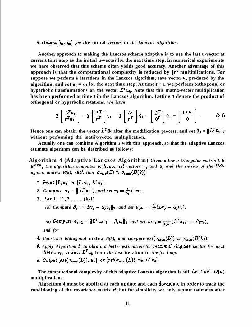
Another approach to making the Lanczos scheme adaptive is to use the last u-vector atcurrent time step as the initial u-vector for the next time step. In numerical experimentswe have observed that this scheme often yields good accuracy. Another advantage of thisapproach is that the computational complexity is reduced by in2 multiplications. Forsuppose we perform k iterations in the Lanczos algorithm, save vector uk produced by thealgorithm, and set & = uk for the next time step. At time t + 1, we perform orthogonal orhyperbolic transformations on the vector LTuk. Note that this matrix-vector multiplicationhas been performed at time t in the Lanczos algorithm. Letting T denote the product oforthogonal or hyperbolic rotations, we have

Hence one can obtain the vector ET& after the modification process, and set 51 = llZTGrl12without performing the matrix-vector multiplication.

Actually one can combine Algorithm 3 with this approach, so that the adaptive Lanczosestimate algorithm can be described as follows:

- Algorithm 4 (Adaptive Lanczos Algorithm) Given a lower triangular matrix L ER nXn, the algorithm computes orthonormal vectors Vj and uj and the entries of the bidi-agonal matrix B(k), such that amax(L) w amax(B(k))

1. hJM&t [L,Ul] Of [L,Ul, LTU1].

2. Compute cy1 = II LTu&, and set v1 =-iI LTul.

3. Forj=l,2 ,..., (k-l)(a) Compute pj = IlLvj - ajujll2, and set uj+l = $(Lvj - ajuj),

(b) Compute aj+l = IILTuj+l - pivjllz, and set vj+l = &(LTuj+l - pjvj),

end for

4. Construct bidiagonal matrix B(k), and compute est(a,,,(L)) = amax(B(k)).5. Apply Algorithm 3, to obtain a better estimation for ma&d singular vector for next

time step, OT Save LTuk from the last iteration in the for loop.6. OUtpUt [&(0max(L)), Uk], Of [est(amax(L)), Uk7LTUk]*

The computational complexity of this adaptive Lanczos algorithm is still (k-l)n2+0(n)multiplications.

Algorithm 4 must be applied at each update and each downdate in order to track theconditioning of the covariance matrix P, but for simplicity we only reprort estimates after

11

each sliding window time step, i.e., after each downdate. Similar modifications can bemade for estimating bmin(L). 0 nce we obtain the estimates for o,,,(L), and gmin(L),then the spectral condition number of the covariance matrix P is approximated by

AS a side benefit, the recursive estimates of Amin and Am,,(P) also provide approx-imate bounds for the power spectral density of the least squares process in the context ofadaptive filtering, as described by Haykin [21], pp. 62-66. The corresponding singular vec-tors also provide useful information in the context of Pisarenko harmonic decomposition,e.g., [23].

4 Comparisons and Numerical ExperimentsIn this section we report on some selected experiments designed to compare the perfor-mance of the adaptive condition estimation scheme, ale, associated with Algorithm 4 withtwo alternative methods, one due to Pierce and Plemmons [31] and called ace and the otherdue to Bischof [5] and called ice. The scheme ace is adaptive and ace requires up to 38nmultiplication per update/downdate sliding window time step, while ice is non-adaptive

- and requires up to 6n2 + O(n) multications - the same as our adaptive Lanczos estimatorale using the secular equation approximations to obtain starting vectors. If the alternativeapproach of using the last u-vector at current time step as the initial u-vector for the nexttime step is employed, then the complexity of ale is reduced to 4n2 + O(n) multiplications.It follows that ace is cheaper than this version of ale only when n 2 7.

Some data provided in by A. Bjijrck, some randomly generated data, and some actualdata from signal processing adaptive filtering are considered in our tests and comparisons.The datasets used the tests are described as follows:

l Random data from A. Bjiirck [8]. This dataset consists of m = 50 observationsof n = 5 components each, randomly generated with a uniform distribution in (0,l).An outlier equal to lo4 is added to p.osition (l&3). A sliding window length of 8 isused.

l Hilbert matrix data Corn A. BjSrck [8]. Again m = 50 observations of n = 5components each are generated. This time the fist 25 observations consist of thefirst 5 columns of the Hilbert matrix of dimension 25, and the same rows in reversedorder as the last 25 observations. A random perturbation, uniformly distributed in(0, lo-'), is added to the 10 middle rows to prevent the sliding window submatrices,which have window length 8, from becoming singular.

l Random ill-conditioned data from Pierce and Plemmons [32]. Here m = 100observations of n = 10 components each is generated with a random distribution in

12

(-50,50). Ill-conditioning is forced by multiplying one component of each observa-tion by low3 to force near column dependency for the sliding window submatrices.The window length is set at 20.

l Signal processing data from the NC State University Center for Commu-nications and Signal Processing. This signal processing data is generated froma well-conditioned second-order autoregressive process. A total of m = 200 obser-vations of n = 5 components each are considered. A sliding window length of 20 isused.

We report only on the performances of ale (in comparison to the alternatives ace andice), in recursively estimating the condition number of the covariance matrix P for eachupdateldowndate step. Our purpose in these tests is to exhibit the reliability and theaccuracy of ale for recursive least squares computations. All experiments were performedusing the Pro-Matlab system [27]. The results of these experiments are given in Figuresl-4. In the graphs, the solid lines represent ale, the dashed lines represent ace, and thedotted lines represent ice. As can be seen from the figures, ale compares very favorablywith ace and ice in terms of accurately tracking the condition number, KS(P), of thecovariance matrix over time.

Acknowledgement The authors wish to thank A. Bjijrck in the Mathematics Depart-ment at Linkoping University, Sweden, for providing test data. We also wish to thankAvinash Ghimikar and Tulay Adali in the N.C. State University Electrical and ComputerEngineering Department for supplying the signal processing data used our tests.

References[l] S.T. Alexander, Adaptive Signal Processing, Springer Verlag, New York (1986).

[2] S.T. Alexander, C.-T. Pan and R.J. Plemmons, Analysis of a recursive least squareshyperbolic rotation scheme for signal processing, Lin. Alg. Appl. Special Issue onElectrical Eng. 98 (1988) 3-40.

[3] K.J. Astrijm and B. Wittenmark, Adaptive Control, Addison-Wesley, Reading MA(1989).

[4] G.J. Bierman, Factorization Methods for Discrete Sequential Estimation,Academic Press, NY (1977).

[5] C.H. Bischof, Incremental condition estimation, SIAM J. on Matrix Anal. andApplic. to appear April (1990).

13

PI

VI

PI

PI

PO1

Pll

P21

- WI

PI

PI

M

PI

P4

PI

C.H. Bischof and G.M. &off, On updating signal subspaces, Tech. Rept., ArgonneNational Lab. September (1989).

A. Bjiirck, Least Squares Methods, in Handbook of Numerical Analysis, P.Ciaxletand J. Lions, eds., Elsevier/North Holland, Amsterdam (1989).

A. Bjiirck, Accurate downdating of least squares solutions, presented at the AnnualSIAM Meeting, held at San Diego, CA (1989).

J.R. Bunch, C.P. Nielson, Updating the Singular Vaule Decomposition, Numer.Math., 31 (1978) 111-129.

J.R. Bunch, C.P. Nielson, and D.C. Sorensen, Rank-One Modification Of the Sym-metric Eigenproblem, Numer. Math. 31 (1978) 31-48.

J.M. Cioffi, Limited precision effects in adaptive filtering, IEEE Trans. on CAS 34(1987) 821-833.

J.M. Cioffi and T. Kailath, Windowed fast transversal filters, adaptive algorithmswith normalization, IEEE Trans. on ACOUS., Speech and Sig. Proc. 33 (1985)607-625.

P. Comon and G.H. Golub, Tracking a few extreme singular values and vectors insignal processing, Stanford Univ. Tech. Rept. NA-89-01 (1989).

R.D. DeGroat and R.A. Roberts, Highly parallel eigenvector update methods withapplications to signal processing, SPIE Adv. Alg. and Arc. for Signal Proc. 696(1986) 62-70.

P.E. Gill, G.H. Golub, W. Murray and M.A. Saunders, Methods for modifying matrixfactorizationa, Math. Comput. 28 (1974) 505-535.

G.H. Golub, Matrix decompositions and statistical calculations, in R.C. Milton andJ.A. Nelder, Eds., Statistical Computation, Academic Press, New York, (1969)365-395.

G.H. Golub, Some modified matrix eigenvalue problems, SIAM Review 15 (1973)318-334.

G.H. Golub and W. Kahan, Calculating the singular values and pseudo inverse of amatrix, SIAM J. Num. Anal. Ser. B2 (1965) 205-224.

G.H. Golub, F.T. Luk and M.L. Overton, A block Lanczos method for computing thesingular values and corresponding singular vectora of a matrix, ACM Transcationon Mathematical Software 7 (1981) 149-169.

14

[20] G.H. Golub and C. V L= oaq Matrix Computations, Johns Hopkins Press, Balti-more, Second Edition (1989).

[21] S. Haykin, Adaptive Filter Theory, Prentice-Hall, Englewood Cliffs, NJ (1986).

[22] C.S. Henkel and R.J. Plernmons, Recursive least squares computations on a hypercubemultiprocessor using the covariance factorization, SIAM J. Sci. Statist. Comp.,to appear (1990).

[23] N.J. Higham, A survey of condition estimators for triangular matrices, SIAM Re-view 29 (1987), 575-596.

[24] Y.H. Hu, Adaptive methods for real time Pisarenko spectrum estimation, Proc.ICASSP, Tampa, FL (1985).

[25] C. Lauczos, An iteration method for the solution of the eigenvalue problem of lineardifferential and integral operators, J. Res. Nat. Bur. Stand. 45 (1950) 255-281.

[26] F. Milinazzo, C. Zala and I. Barrodale, On the rate of growth of condition numbersfor convolution matrices, IEEE Trans. ACOUS., Speech and Sig. Proc. 35 (1987)471-475.

- [27] C. Moler, J. Little and S. Bangert, Pro-Matlab Users Guide, The Mathworks,Sherbom, MA (1987).

[28] M. Moonen, P. van Dooren and J. Vandewalle, Parallel updating algorithms, part one:IThe ordinary singular value decomposition, preprint (1989).

[29] M. Morf and T. Kailath, Square root algorithms and least squares estimation, IEEETrans. on Automatic Control 20 (1975) 487-497.

[30] C.-T. Pan and R.J. Plemmons, Least squares modifications with inverse factorizationa:parallel implications, Computational and Applied Math. 27 (1989) 109-127.

[31] D.J. Pierce and R.J. Plemmons, Fast adaptive condition estimation, preprint (1990).

[32] D.J. Pierce and R.J. Plemmons, Fast adaptive condition estimation for RLS in signalprocessing, I: Exponential weighting, submitted (1990).

[33] D.J. Pierce and R.J. Plemmons, Fast adaptive condition estimation, II: Sliding win-dows for RLS in signal processing, in preparation (1990).

[34] R.J. Plemmons, Recursive least squares computations, Proc. Inter. Conf. on Math.in Networks and Syst., Birkhauser Boston, Inc., to appear (1990).

[35] S. Sastry and M. B do son, Adaptive Control: Stability, Convergence, and Ro-bustness, Prentice-Hall, Englewood Cliffs, NJ, (1989).

15

[36] R. C. Thompson, The Behavior of Eigenvalues and Singular Values under Perturba-tions of Restricted Rank, Linear Algebra and Its Applications 13 (1976) 69-78.

16

ale Condition Estimate (x), Actual (-)1 I I I , 1 I I

2.6 IRatio : Actual/Estimate, ale (-), ace (--), ice (:)

I 1 I I I I I ,

2.4t

2.2 -

1.8 -

1.6 -

1.4 -

1.2 -

l -

1I

:I-

:

::

:

0.8l I I I I L 1 I I I0 5 lo 15 20 25 30 35 40 45 50

Random Data by Bjorck - Time Scale

Figure 1: Comparison of ale with ace and ice on random data with outlier fromA. Bjiirck.

17

2.Ratio : Actual/Estimate, ale (-), ace (--), ice (:)

I I 1 , 1 I I ., I I -I I : II : II I I1I : I

I- I I: :I III I :I II I III

i - I

. . .

.

ale Condition Estimate (x), Actual (-)I 1 I 1 I r I I Ilog-

10’ -

106 -

102

10’

100’ I I I I I I I I I0 5 10 15 20 25 30 35 40 45 50

,I I I0.8 1 1 1; I I I I I I 1 I ,0 5 10 20 25 30 35 40 45 50

tilbeti Ma& Data by Bjorck - Time Scde

Figure 2: Comparison of ale with ace and ice on Hilbert matrix data from A.Bjiirck.

18

ale Condition Estimate (x), Actual (-)I I I I I I I I -I

10'1 I I I I I 1 I I I I0 10 20 30 40 50 60 70 80 90 100

2

1.8

1.6 I -

J

0.8-0

Ratio : Actual/Estimate, ale (-), ace (--), ice (:)

1 1 1 I 1 I 1 I I

10 20 30 40 50 60 70 80 90 100

Ill-Conditioned Random Data - Time Scale

. . ..

G

Figure 3: Comparison of ale with ace and ice on random moderately ill-conditioned data from Pierce and Plemmons.

19

ale Condition Estimate (x), Actual (-)

20 40 60 80 100 120 140 160 180 200

2

1.8

1.6

3 142 ’

1.2

1

0.8

Ratio : Actual/Estimate, ale (-), ace (--), ice (:)

:: I I: :: : I :

I I 1 I I I 1 I I

20 40 60 80 100 120 140 160 180 200

NCSU Signal Processing Data - Time Scale

Figure 4: Comparison of ale with ace and s’ce on signal processing data.

20