adaptive memory programming for constrained …leeds-faculty.colorado.edu/glover/fred pubs/416 - amp...

Adaptive Memory Programming for Constrained Global Optimization

LEON LASDON Information, Risk, and Operations Management Department The University of Texas at Austin, USA [email protected]

ABRAHAM DUARTE Departamento de Ciencias de la Computación Universidad Rey Juan Carlos, Spain [email protected]

FRED GLOVER OptTek Systems, Inc. Boulder, CO 80302, USA [email protected]

MANUEL LAGUNA Leeds School of Business University of Colorado at Boulder [email protected]

RAFAEL MARTÍ Departamento de Estadística e Investigación Operativa Universidad de Valencia, Spain [email protected]

Abstract

The problem of finding a global optimum of a constrained multimodal function has been the subject of intensive study in recent years. Several effective global optimization algorithms for constrained problems have been developed; among them, the multistart procedures discussed in Ugray et al. (2007) are the most effective. We present some new multistart methods based on the framework of adaptive memory programming (AMP), which involve memory structures that are superimposed on a local optimizer. Computational comparisons involving widely used gradient-based local solvers, such as Conopt and OQNLP, are performed on a testbed of 41 problems that have been used to calibrate the performance of such methods. Our tests indicate that the new AMP procedures are competitive with the best performing existing ones.

Original version: May 24, 2009 First Revision: October 20, 2009 Second Revision: November 5, 2009

mailto:[email protected]�





AMP for Constrained Global Optimization / 2

1. Introduction The constrained continuous global optimization problem (P) may be formulated in a general form as follows:

(P) minimize f(x) subject to: G(x) ≤ b x∈S ⊂ Rn

where x is an n-dimensional vector of continuous decision variables, G is an m-dimensional vector of constraint functions, and without losing generality the vector b contains upper bounds for these functions. The set S is defined by simple bounds on x, and we assume that it is closed and bounded, i.e., that each component of x has a finite upper and lower bound. The objective function f and the constraint functions G are assumed to have continuous first partial derivatives at all points in S. There are many effective methods, such as Conopt, Snopt and Knitro, most of them requiring gradients of the problem functions, for finding local solutions to (P). In this paper we propose memory structures (Glover 1989, Duarte et al. 2009) that can be superimposed to these methods to drive the search on a long term horizon to solve the global optimization problem. These structures use a local solver to generate trial solutions which are candidates for a global optimum, where as customary the best feasible candidate is retained as the overall “winner”. The local solver may be gradient-based, or may be a “black box” algorithm as typically used in simulation optimization (see, e.g., April et al., 2006; Better, Glover and Laguna, 2007). The local solver used here is Conopt, a GRG algorithm (Smith and Lasdon, 1992), described in (Drud 1994). This gradient-based algorithm is known to have a superlinear convergence rate, and has an excellent combination of reliability and efficiency, when applied to both small and large sparse smooth NLP’s. Our adaptive memory structure will guide the selection of starting points for the local solver. Specifically, we propose two different Adaptive Memory Programming (AMP) approaches (Glover and Laguna, 1997); the first one, described in Section 2, is based on a tabu tunneling strategy and the second one, described in Section 3, is based on a pseudo-cut strategy. Both are designed to prevent the search from being trapped in local optima. In Section 4, we describe the GAMS implementation of both AMP approaches. Section 5 is devoted to our computational experiments on 41 hard problems from the literature (see Ugray et al. 2007). We will show that the tabu tunneling strategy is able to outperform the state-of-the-art methods for constrained global optimization. On the other hand, the pseudo-cut strategy obtains lower quality results on average (as compared to the tunneling strategy), although it substantially improves the Conopt method. We also show that the pseudo-cut strategy can be coupled with the tunneling method for improved outcomes. The paper finishes with relevant conclusions.


2. Tabu Tunneling Method Metaheuristic methodologies diversify a search to march beyond local optimality in the quest for a global optimum. Applying a local optimizer to points in the same region of the solution space may result in repeatedly obtaining the same local optimum, unless additional constraints are imposed or the evaluation criterion is modified. In this section we propose an adaptive modification of the objective function to perform multiple searches with the goal of reaching different local optima of the original objective function. Our approach modifies and extends the global optimization tunneling method (TM) of Levy and Gomez (1985) for unconstrained problems. The original TM approach consists of two phases, minimization and tunneling, which are alternated until a cutoff point is reached. From a given starting point s0, the minimization phase applies a descent algorithm to find a local optima s. The tunneling phase is designed to obtain a good starting point for the next minimization phase. The objective is to obtain a point t with a value as good as s (f(t) ≤ f(s)) in a different basin of attraction. Therefore if we apply the descent method from t we can obtain now a solution w better than s and t as shown in Figure 1.

Figure 1. Tunneling approach

The objective of the tunneling problem must therefore be constructed so that its minimization leads to points which both improve the original function f(x) and are distant from the current solution s. A standard tunneling function T(x,s,λ) is given by the expression:

λλsx

sfxfsxT−

−=

)()(),,(

where λ is positive. Levy and Gomez proposed that an equation-solving method be applied to seek a point where T(x,s,λ) = 0. As mentioned in Murray and Ng (2002), a pure tunneling method may fail to find a point t satisfying f(t) ≤ f(s) in a single iteration. To overcome this limitation, and to extend the method to constrained problems, our tabu tunneling method (TTM), implements a short

s0 s t w

tunneling


term memory strategy to perform multiple iterations in search for such a point t, as follows: 1. Since it is difficult to find a point t different from a local solution s satisfying

f(t) ≤ f(s) in a single application of a local solver, we have developed a multistep process for this purpose, which we call the tunneling loop. We define a TabuList of points from which to move away, including both the most recent local solution of the original problem P, and recent solutions of tunneling subproblems which failed to achieve the desired condition.

2. To enforce movement away from several points, we redefine the denominator of T to

be the product of distances from the points in TabuList. 3. Rather than making the current best objective value Best_f the target to be achieved

by the tunneling loop, we define an aspiration value for the objective function which is slightly less than Best_f;

aspiration = Best_f - ε1·(1+abs(Best_f ))

where the default value of ε1 is 0.02, and the additive unity term is included to ensure a nonzero reduction when Best_f is zero, and a significant reduction when abs(Best_f) is very small. With these elements, our tunneling function TTf is:

∏∈

−=

TabuListsi

i

sxdistaspirationxfxTTf 2

2

)),(())(()(

For simplicity, we do not indicate explicitly the dependence of TTf on aspiration and the points in TabuList. This function has a global minimum of zero at any feasible point where f = aspiration, and minimizing this expression tends to move away from all points in TabuList.

4. To accommodate constraints other than simple bounds, we redefine the tunneling

subproblem (TP) to include all the constraints of the original problem:

(TP) minimize TTf(x) subject to: bG(x) ≤ Sx ∈ 5. Since TTf is not defined at any of the points in TabuList, the starting point for (TP)

cannot be in TabuList. Further, if the local solver used to solve (TP) encounters any point in TabuList during its solution process, it may terminate due to a domain violation error. This happened when using Conopt in a number of experiments, for the following reasons. Since Conopt is a “feasible point” solver, if the starting point is not feasible, it tries to find a feasible point using a standard phase 1 procedure, just


as the Simplex algorithm for linear programming would do. This phase 1 procedure ignores the given objective and substitutes an objective equal to the sum of constraint violations. Thus there is no mechanism in phase 1 to avoid the points in TabuList, and we found that in many cases where an infeasible starting point was supplied for (TP), Conopt’s phase 1 terminated with a feasible solution equal to a point in TabuList. When it attempted to use this point to initiate minimization of TTf in phase 2, this triggered a fatal error message and Conopt terminated.

The only sure way to avoid the problem in point 5 above is to provide the local solver with a feasible starting point not equal to any of the points in TabuList. We have found that an effective way to do this is to first randomly perturb away from the current local solution (the newest point in TabuList) to a (generally infeasible) point x0, and then find the feasible point closest to x0 by solving the following Projection Problem

(PP) minimize 20xx −

subject to: bG(x) ≤

Sx ∈ In all constrained problems solved thus far, containing hundreds of instances of (PP), this strategy has never failed to provide a suitable starting point for (TP). As in a variety of simple tabu search implementations, we maintain TabuList as a circular list. After each solution of the tunneling problem defined above, we add the solution to that problem to the list, and if the size of the new list exceeds the limit (called TabuTenure in the following description), some old point is dropped from the list. We have experimented with dropping the oldest element, dropping the element farthest from the point just added to the list, and dropping the oldest element whose distance from the point just added is larger than a specified fraction of the largest distance. Results comparing these alternatives are discussed later. Figure 2 provides a pseudo-code description of our tabu tunneling algorithm, in which LS is the local search or descent algorithm for constrained global optimization. In line 5 we use the expression s = LS(s0, f(x),G,S) to indicate that we optimize problem (P) (i.e., the minimization of f(x) subject to the original constraints G and S) from the initial point s0 with the LS optimizer. Similarly, in line 11 the expression s = LS(s', TTf(x,aspiration),G,S) indicates that we solve problem (TP) with objective function TTf(x) subject to the original constraints G and S from the initial point s' using LS. Also, s = LS(x0,

20xx − ,G,S) in line 12 represents solving the projection problem

(PP) starting from x0 using LS. The While-loop (lines 9 to 18) in Figure 2 performs the tunneling approach, and is repeated TotalIter times. Note that in line 15 we update the TabuList, which means that we add the point s obtained in line 14 and drop some other point from the list. The tunneling loop ends when the tunneling solution has an f value less than or equal to


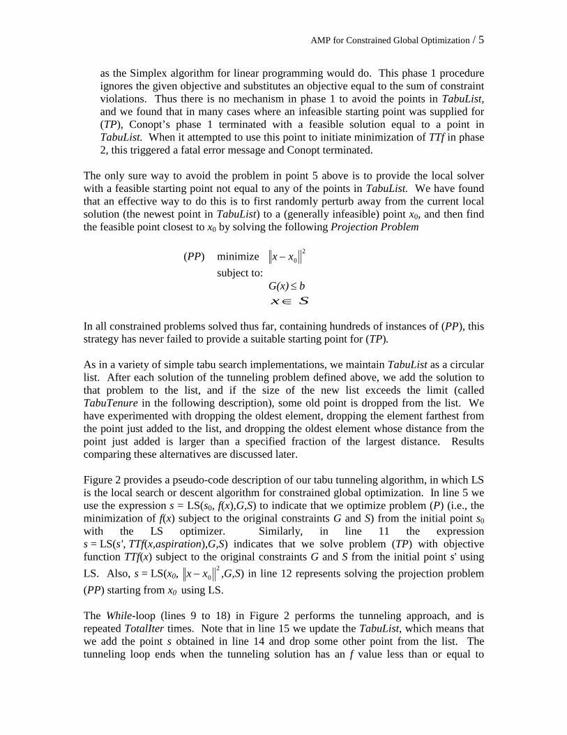
Best_f, or when the iteration limit MaxIter is reached. At this point the search can either terminate (if the GlobalIter counter reaches its maximum, TotalIter) or continue performing a new iteration in Step 5 from s0 (the latest local optimum obtained with the tunneling minimization).

Figure 2. Pseudo-code of the Tabu Tunneling method

3. The Tabu Cutting Method The pseudo-cut strategy (Glover 2008) is based on generating hyperplanes that are orthogonal to selected rays (half-lines) originating at a point x′ and passing through a second point x″, so that the hyperplane intersects the ray at a selected point xo. We employ a simplified variant of the method here. The half-space that forms the pseudo-cut is then produced by the associated inequality that excludes x′ and x'' from the admissible half-space. Let x identify points on the ray originating at x′ that passes through x″:

Initialization 1. s0 = user-provided initial solution 2. Let TabuList be the memory list with TabuTenure size 3. Let Best_f be the value of the best solution found (initialized to ∞) 4. GlobalIter = 0 Minimization of original objective starting from s0 5. s = LS(s0, f(x),G,S ) 6. TabuList = {s} If ( f(s) < Best_f)

7. Best_f = f(s) Tabu Tunneling 8. i = 0, improve = 0 While (i < MaxIter and improve = 0) // default value of MaxIter = 5

9. r = vector with components uniformly distributed on [-1,1] 10. rs /*2εβ = // default value of 2ε = 0.1

11. rsx *0 β+=

12. s' = LS(x0, 2

0xx − ,G,S)

13. aspiration = Best_f - ε1·(1+abs(Best_f )) // default value of ε1=0.02 14. s = LS(s', TTf(x,aspiration),G,S ) 15. Update the TabuList If ( f(s) ≤ Best_f)

16. Best_f =f(s) 17. improve=1

18. i = i + 1 19. GlobalIter = GlobalIter + 1 If (GlobalIter = TotalIter) // default value of TotalIter = 20

20. STOP Else

21. s0= s and GOTO Step 5.


x = x′ + λ(x″ – x′), λ ≥ 0 A hyperplane orthogonal to this line may then be expressed as (x″ – x′) x = b where b is an arbitrary constant. Let xo be a point in the ray (xo=x′+λo(x″–x′)) then, the inequality (pseudo-cut) that excludes x′ and x'' and includes xo is given by:

(x″ – x′) x ≥ (x″ – x′) x0 We make use of this inequality or pseudo-cut (shown in Figure 3) called pcut(x′, x″, x0) within a two-stage process. In the first stage, x′ represents a point that is used to initiate a current search by the local search or descent method LS, and x″ is the point obtained. We can use Conopt or any other local optimizer for constrained optimization as the descent method LS and employ the same notation introducing in the previous section (i.e. x″ = LS(x′,f(x),G,S).

Figure 3. Pseudo-cut representation

Once we obtain the point x″ with the local optimizer, we generate a new point xo. The point xo can be simply computed as xo = x′ + m(x″ – x′) where m is a multiple of the distance between x′ and x″. We now add the pseudo-cut pcut(x′, x″, x0) to the set of constraints of the problem and solve the extended problem by applying the local search method from xo to obtain y. The objective is to escape from the local optima x″ obtained with LS and explore a new region. Using our previous notation:

y = LS(xo, f(x),G∪{pcut(x′, x″, x0)}, S). We repeat this first stage of the process iteratively. We make now x′ = xo, x″ = y, compute a new point xo and create the associated pseudo-cut. Since we want to solve now the original problem with two pseudo-cuts (the one introduced in the previous iteration and the new one), we create a short term memory structure TabuCutList to store the recent cuts (we limit its size to the TabuTenure latest cuts). As it is customary in tabu search implementations the short term memory is implemented as a circular list in which we drop from the list the first cut (the oldest one) when we introduce a new one, thus keeping the size TabuTenure constant. In this way we create a diversification mechanism to avoid the exploration of areas in the solution space recently visited.

x′ x″ xo

Pseudo-cut (x″ – x′) x ≥ (x″ – x′) xo

Ray x′ + λ(x″ – x′)


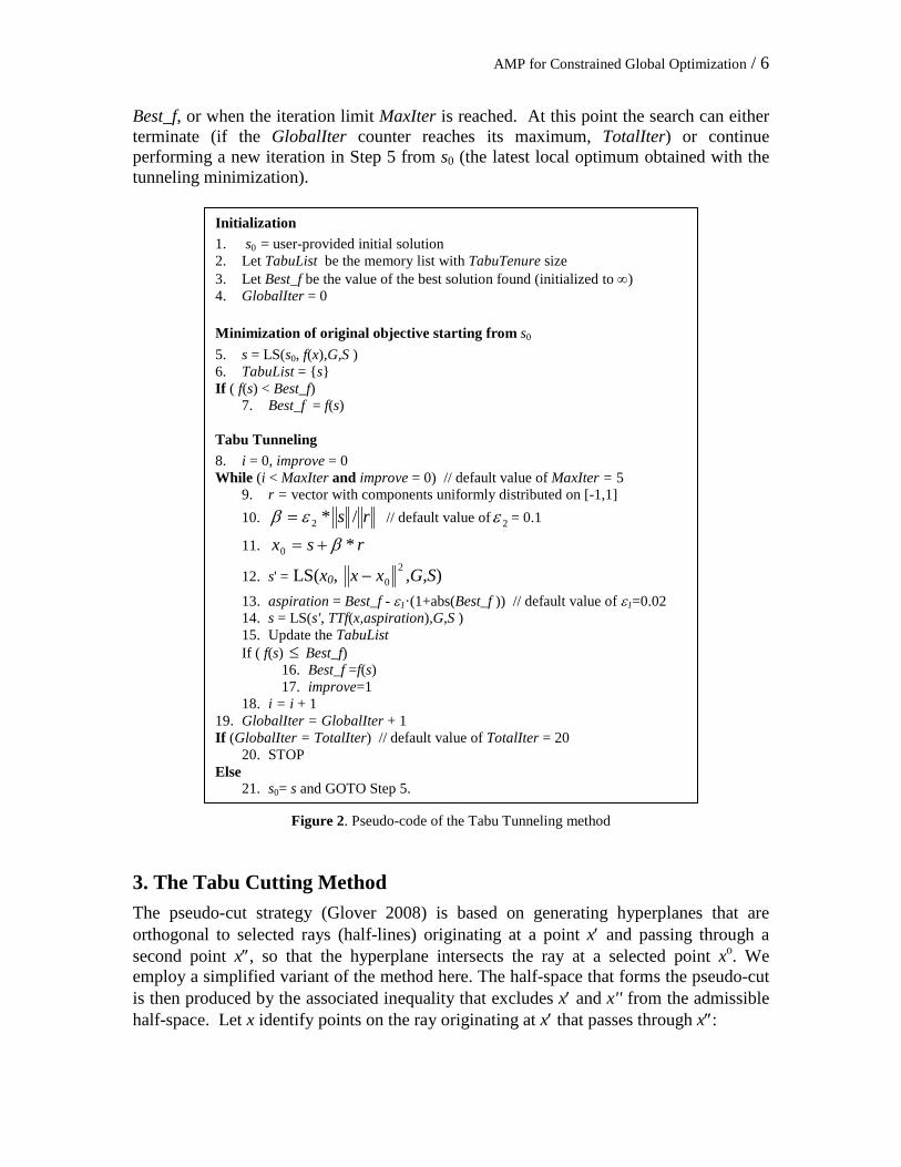
Figure 4. Second stage of the method

In the process above, we can eventually obtain the point y lying on the hyperplane associated with the current pseudo-cut pcut(x′, x″, x0), as shown in Figure 4:

y = LS(x0, f(x),G∪{ pcut(x′, x″, x0)}, S) In this case, we resort to the second stage of our algorithm, in which we replace this cut with a new one. To this end we define a new point xo in the segment from x″ to y: xo = x″+m(y – x″). Note that the multiple m is selected to be greater than 1 in the first stage and less than 1 in this second stage. Then the new cut is given by the expression:

(y – x'′) x ≥ (y – x'′) x0 As in the first stage, we solve now the problem with this cut (that we called pcut(x″, y, x0)). In terms of our notation, we apply LS(x0, f(x),G∪{pcut(x″, y, x0)}, S ). If the final point of this local search application does not lie on the hyperplane associated with the current cut, we return to Stage 1 of the process; otherwise we perform a new iteration of Stage 2. At a given iteration of the tabu cutting method (TCM) we apply the local search method LS from x′, to solve the original problem in which we added all the cuts in the TabuCutList. That is, we obtain y by applying the local optimizer with the following parameters:

y = LS(x′, f(x),G ∪ TabuCutList, S ) Figure 5 shows a pseudo-code of TCM that is designed to repeat this process, adding one cut at a time while dropping the oldest one from the list of active cuts and applying the local search method for MaxIter iterations.

x′ x″ xo y

Pseudo-cut pcut(x', x'', x0) (x″ – x′) x ≥ (x″ – x′) xo

Ray x′ + λ(x″ – x′)


Figure 5. Pseudocode of the pseudo-cut method

Steps 10 to 21 in Figure 5 show the main loop of our Tabu Cutting Method. We can identify the following three cases when applying the local search method LS from x0 to obtain y. Let pcut(x′, x″, x0) be the latest cut added to TabuCutList (Step 11 in the procedure). Depending where y lies we can distinguish:

A. y is equal to x0. This case is identified in the IF statement above step 16 (||y– x0|| < minDist). This indicates that the local search method is not able

Initialization 1. Let TabuCutList be the memory list of pseudo-cuts with TabuTenure size 2. Let m=0.1, minDist=0.0001, Iter1=Iter2=0, MaxIter = 5 and GlobalIter= 20 3. Let x′ be a user-provided initial solution, Best_f = f(x′), l and u the lower and upper bounds

of x respectively.

While (Iter1 < GlobalIter) 4. TabuCutList = ∅ 5. improved = FALSE 6. pert = m 7. x′′ = LS(x′, f(x),G,S ) If (f(x′′) < Best_f)

8. Best_f = f(x′′) 9. x0 = x′ + (1 + pert)⋅( x′′ – x′)

While (Iter2 < MaxIter and NOT improved and || x′′ – x′ || > minDist) 10. Remove from TabuCutList the cuts violated at x0 and the old cuts (TabuTenure) 11. Add to TabuCutList the cut pcut(x′, x″, x0): (x″ – x′) x ≥ (x″ – x′) x0 12. y = LS(x0, f(x),G∪ TabuCutList, S ) If (f(y) < Best_f)

13. improved = TRUE 14. Best_f = f(y) 15. go to 21

If (||y – x0|| < minDist) 16. pert = pert + m

Else 17. pert = m

// Case A If (|| y – x0|| < minDist )

18. x0 = x′ + (1 + pert)*( x′′ - x′) //Case B Else If (y verifies pcut(x′, x″, x0) with equality)

19. x′ = x′′; x′′ = y; x0 = x′ + (1 - pert)*( x′′ - x′)

//Case C Else

20. x′ = x0; x′′ = y; x0 = x′ + (1 + pert)*( x′′ - x′) 21. Iter2 = Iter2 + 1

22. x′ = y + r (u - l) where r is a random number in [0,1]. 23. Iter1 = Iter1+1


to generate a new solution, probably because the search remains in the same basin of attraction. We therefore add a new cut farther away from x″. Then, in Step 16 we increase the value of pert, and resort to Step 18 to compute a new point x0 as shown in Figure 6.

Figure 6. A-Strategy

B. y verifies the cut pcut(x′, x″, x0) with equality, (x″ – x′) x = (x″ – x′) x0, but it is different to x0 as shown in Figure 7. This indicates that we probably would find better solutions closer to x″ (in the infeasible region of the added cut). This is the Stage 2 of the method. In Step 19 we define a new point x0 closer to x″ (according to pert = m set in Step 17) and in Step 10 we remove this cut.

Figure 7. B-Strategy

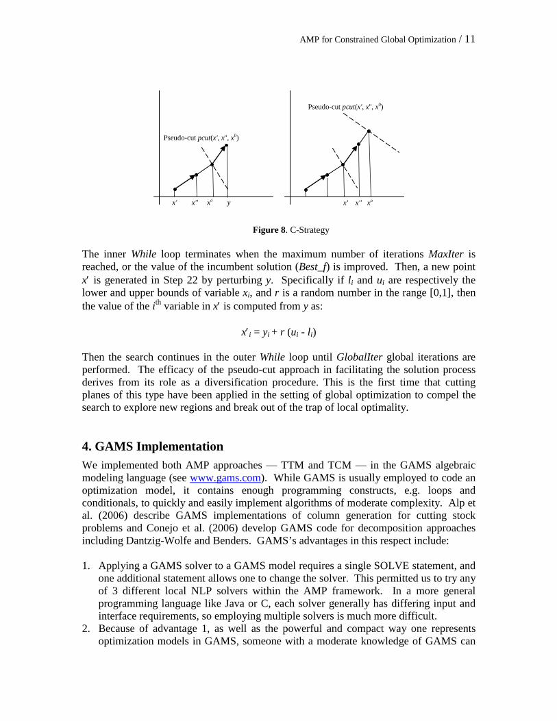
C. y strictly verifies the cut with inequality: (x″ – x′) x > (x″ – x′) x0. We therefore have obtained a good solution (y) in the feasible region of the cut pcut(x′, x″, x0). So we keep this cut in the TabuCutList and repeat the process from y. Then, in Step 20 we exchange the roles of the points (x′ = x0; x′′ = y), and compute a new point x0. Figure 8 shows this case.

x' x'' x0 y

Pseudo-cut pcut(x', x'', x0)

x' xo x’’


x' x'' xo


x' x'' xo



Figure 8. C-Strategy

The inner While loop terminates when the maximum number of iterations MaxIter is reached, or the value of the incumbent solution (Best_f) is improved. Then, a new point x′ is generated in Step 22 by perturbing y. Specifically if li and ui are respectively the lower and upper bounds of variable xi, and r is a random number in the range [0,1], then the value of the ith variable in x′ is computed from y as:

x′i = yi + r (ui - li) Then the search continues in the outer While loop until GlobalIter global iterations are performed. The efficacy of the pseudo-cut approach in facilitating the solution process derives from its role as a diversification procedure. This is the first time that cutting planes of this type have been applied in the setting of global optimization to compel the search to explore new regions and break out of the trap of local optimality. 4. GAMS Implementation

We implemented both AMP approaches — TTM and TCM — in the GAMS algebraic modeling language (see www.gams.com). While GAMS is usually employed to code an optimization model, it contains enough programming constructs, e.g. loops and conditionals, to quickly and easily implement algorithms of moderate complexity. Alp et al. (2006) describe GAMS implementations of column generation for cutting stock problems and Conejo et al. (2006) develop GAMS code for decomposition approaches including Dantzig-Wolfe and Benders. GAMS’s advantages in this respect include: 1. Applying a GAMS solver to a GAMS model requires a single SOLVE statement, and

one additional statement allows one to change the solver. This permitted us to try any of 3 different local NLP solvers within the AMP framework. In a more general programming language like Java or C, each solver generally has differing input and interface requirements, so employing multiple solvers is much more difficult.

2. Because of advantage 1, as well as the powerful and compact way one represents optimization models in GAMS, someone with a moderate knowledge of GAMS can

x' x'' xo y


x' x'' xo


http://www.gams.com/�


implement and debug an algorithm such as the three referred to in the references above or AMP in a few days.

3. The algorithm can be applied to any problem already coded in GAMS. Since GAMS has a library currently containing 413 smooth NLP’s (called GLOBALLIB), most with multiple distinct local optima, solution methods can be applied to a fairly large set of problems, many of which are large and/or difficult. GLOBALLIB can be downloaded at http://www.gamsworld.org/global/globallib.htm

4. GAMS is already interfaced to four powerful and widely used global optimizers, OQNLP, BARON, LGO, and LINDOGLOBAL, so these can also be applied to any problem solvable by the AMP GAMS implementation, and the results are directly comparable.

5. AMP can be started from the final solution of any other GAMS solver, showing what happens when the two are combined sequentially. The experiments below include a set starting with OQNLP, then applying TTM, as well as TTM coupled with TCM.

A significant disadvantage of the GAMS implementation of TTM arises because the objective of problem (TP), the function TTf(x), depends on x not only through the original objective f(x) but also directly because of its denominator. Thus models with different names for the variables x require different GAMS expressions to compute the denominator of TTf. Hence the algorithm implementation depends on the model, restricting the number of problems to which this implementation can be easily applied. 5. Computational Experiments This section describes the results obtained applying the GAMS implementation of TTM and TCM described above. All experiments were conducted on a Dell Latitude D820 computer with an Intel T2500 CPU running at 2.0 GHz with 1.9 GB of RAM. The GAMS version used was 22.5. Ugray et al. (2007) performed extensive experimentation with the OQNLP multistart algorithm on a large set of 142 global optimization test problems from Floudas et al. (1999). The GAMS models of these test problems are in the well-known GAMS GLOBALLIB, available at http://www.gamsworld.org/global/globallib/globalstat.htm. We have identified 26 hard instances in the set of 142. Since we view this work as an extension of the method of Ugray et al. (2007), we test our TTM and TCM procedures on the 26 problems for which OQNLP encountered difficulties. We have extended our test set to include 15 instances and complement the previous 26. Specifically, from instance EX2_1_1 in Ugray et al. (2007), we consider the entire family EX2_1_n in GLOBALLIB, which includes EX2_1_1, EX2_1_2, EX2_1_3, EX2_1_4 and EX2_1_5. Therefore our collection of 41 instances contains 6 families of problems: EX2_1_n, EX2_1_7_n, EX3_1_n, EX8_6_1_n, EX8_6_2_n and EX9_2_n.

http://www.gamsworld.org/global/globallib.htm�

http://www.gamsworld.org/global/globallib/globalstat.htm�


Problem Vars.

Linear constraints

Nonlinear constraints

Best known objective

Conopt value

Conopt Gap No.

1 EX2_1_1 5 1 0 -17 0.00 100.00% 2 EX2_1_2 6 2 0 -213 -213.00 0.00% 3 EX2_1_3 13 9 0 -15 -12.66 15.63% 4 EX2_1_4 6 5 0 -11 -11.00 0.00% 5 EX2_1_5 10 11 0 -268.0146 -268.02 0.00% 6 EX2_1_6 10 5 0 -39.00 -21.25 45.51% 7 EX2_1_8 24 10 0 15639.00 19971.00 27.70% 8 EX2_1_9 10 1 0 -0.375 -0.33 11.20% 9 EX2_1_7_1 20 10 0 -394.75 -38.52 90.24%

10 EX2_1_7_2 20 10 0 -884.75 -794.77 10.17% 11 EX2_1_7_3 20 10 0 -8695.01 -6012.66 30.85% 12 EX2_1_7_4 20 10 0 -754.75 -633.44 16.07% 13 EX2_1_7_5 20 10 0 -4150.41 -407.43 90.18% 14 EX3_1_1 8 3 3 7049.248 7049.25 0.00% 15 EX3_1_2 5 0 6 -30665.525 -30665.53 0.00% 16 EX3_1_3 6 4 2 -310.00 -132.00 57.42% 17 EX3_1_4 6 4 2 -4.00 -4.00 0.00% 18 EX8_6_1_5_ 15 0 10 -9.10 -9.10 0.00% 19 EX8_6_1_10 30 0 45 -28.42 -26.02 8.44% 20 EX8_6_1_15 45 0 105 -52.32 -47.45 9.31% 21 EX8_6_1_20 60 0 190 -77.18 -70.67 8.43% 22 EX8_6_1_25 75 0 300 -102.37 -95.47 6.74% 23 EX8_6_1_30 90 0 435 -128.29 -113.75 11.33% 24 EX8_6_1_40 120 0 780 -184.16 -168.34 8.59% 25 EX8_6_1_50 150 0 1225 -241.67 -232.79 3.67% 26 EX8_6_2_5_ 15 0 0 -9.30 -9.30 0.00% 27 EX8_6_2_10 30 0 0 -31.89 -31.07 2.57% 28 EX8_6_2_15 45 0 0 -63.16 -63.16 0.00% 29 EX8_6_2_20 60 0 0 -97.42 -97.42 0.00% 30 EX8_6_2_25 75 0 0 -136.07 -135.03 0.76% 31 EX8_6_2_30 90 0 0 -177.58 -177.46 0.07% 32 EX8_6_2_40 120 0 0 -268.39 -267.74 0.24% 33 EX8_6_2_50 150 0 0 -366.64 -366.64 0.00% 34 EX9_2_1 11 5 4 17 25.00 47.06% 35 EX9_2_2 11 7 4 100 100.00 0.00% 36 EX9_2_3 17 9 6 0 5.00 0.00% 37 EX9_2_4 9 5 2 0.5 0.50 0.00% 38 EX9_2_5 9 4 3 5 26.00 420.00% 39 EX9_2_6 17 6 6 -1 -1.00 0.00% 40 EX9_2_7 11 5 4 17 25.00 47.06% 41 EX9_2_8 5 3 2 1.5 1.50 0.00%

Total 1069.27%

Table 1. Problem characteristics Table 1 shows the characteristics of the 41 problems employed in our experimentation, providing the name, number of variables, number of linear and nonlinear constraints, best


known objective value, and the value obtained when running the Conopt solver from the starting point provided in the GAMS model (Conopt Value). The EX2_1_n family contains 8 problems (1–8) with concave quadratic objective function and linear constraints. The EX2_1_7_n is a sub-family of the previous family with 5 problems (9-13) all with 20 variables and 10 linear constraints. The EX3_1_n family contains 4 problems (14-17) with quadratic objective function and linear and nonlinear constraints. The “atom energy” problems in families EX8_6 (18-33) choose the locations of a cluster of n particles to minimize the potential energy of the cluster, using two different potential energy functions, called Lennard-Jones (EX8_6_1_n) and Morse (EX8_6_2_n). The decision variables are the (x,y,z) coordinates of each particle. Particle 1 is located at the origin, and three position components of particles 2 and 3 are fixed, so each family of problems has 3n variables, with 6 of them fixed. These problems have many local minima, and their number increases rapidly with problem size, n, so they constitute a good test for global optimization algorithms. Eight problems from each set are solved, with n ranging from 5 to 50. The Lennard-Jones series has many nonlinear constraints, imposed to insure that a division by zero in the objective (which occurs when two or more particles occupy the same point) is avoided, and all have simple bounds. None of these constraints are active at any local solution, so both series are “essentially unconstrained”. The problems in the EX8_6_2_n family are unconstrained but extremely hard. Finally, the EX9_2_n family contains 8 problems (34-41) with bi-level quadratic objective and linear and nonlinear constraints. The last column in Table 1 shows the Conopt “gap”, the percentage difference between the best known objective value and the final Conopt objective value. Conopt alone is able to achieve the best known objective value in 16 of these 41 problems, and 20 of Conopt’s solutions have a gap greater than 5%. The sum of the gaps is 1069.27%. 5.1. Base Case Runs Table 2 shows the results obtained with the TTM and TCM methods. It also shows the results obtained with a multi start method, MS-Conopt, in which Conopt is launched from random initial points. The “Best value” columns in Table 2 show the objective value of the best solution found by each method, and Gap is the percentage difference between the best known objective function value and the objective function value corresponding to the best solution found by each method. For each of these three methods, Table 2 includes the CPU times in seconds. The last row in this table computes the sum of the best values, the total gap and the average CPU times.


MS-Conopt TTM TCM Problem number

Best value Gap

CPU Time

Best value Gap

CPU Time

Best value Gap

CPU Time

1 -16.50 2.94% 12.58 -17.00 0.00% 19.07 -16.00 5.88% 4.27 2 -213.00 0.00% 11.26 -213.00 0.00% 20.67 -213.00 0.00% 4.29 3 -15.00 0.00% 37.15 -15.00 0.00% 37.22 -15.00 0.00% 5.04 4 -11.00 0.00% 12.57 -11.00 0.00% 40.54 -11.00 0.00% 5.17 5 -268.02 0.00% 11.97 -268.02 0.00% 38.9 -268.02 0.00% 6.07 6 -39.00 0.00% 36.62 -39.00 0.00% 34.3 -39.00 0.00% 12.21 7 15639.00 0.00% 36.86 15639.00 0.00% 37.91 15639.00 0.00% 18.87 8 -0.38 0.00% 36.29 -0.38 0.00% 38.18 -0.38 0.00% 5.38 9 -394.75 0.00% 43.95 -394.75 0.00% 39.66 -394.75 0.00% 20.73 10 -884.75 0.00% 41.14 -884.75 0.00% 46.6 -850.17 3.91% 4.73 11 -8695.01 0.00% 43.14 -8695.01 0.00% 39.18 -7542.36 13.26% 5.15 12 -754.75 0.00% 38.57 -754.75 0.00% 40.59 -633.45 16.07% 23.46 13 -4150.41 0.00% 37.71 -4150.41 0.00% 40.74 -1768.14 57.40% 20.11 14 7049.25 0.00% 28.72 7049.25 0.00% 42.78 7049.25 0.00% 6.01 15 -30665.54 0.00% 39.31 -30665.54 0.00% 37.23 -30665.54 0.00% 5.77 16 -310.00 0.00% 36.51 -310.00 0.00% 33.82 -310.00 0.00% 180.4 17 -4.00 0.00% 36.66 -4.00 0.00% 19.13 -4.00 0.00% 6.16 18 -9.10 0.00% 47.65 -9.10 0.00% 43.34 -9.10 0.00% 6.59 19 -28.42 0.00% 106.29 -28.42 0.00% 49.9 -27.55 3.06% 5.72 20 -52.32 0.00% 178.1 -52.32 0.00% 92.92 -52.32 0.00% 8.23 21 -77.18 0.00% 472.12 -77.18 0.00% 122.2 -75.60 2.05% 10.61 22 -99.20 3.09% 180.37 -101.78 0.58% 169.89 -101.88 0.48% 16.26 23 -125.20 2.41% 316.98 -127.38 0.71% 296.49 -125.01 2.56% 19.65 24 -177.75 3.48% 661.56 -181.34 1.53% 611.38 -178.94 2.83% 40.67 25 -239.17 1.03% 1250.15 -237.12 1.88% 1215.11 -237.12 1.88% 68.47 26 -9.30 0.00% 16.55 -9.30 0.00% 43.59 -9.30 0.00% 5.66 27 -31.89 0.00% 17.76 -31.89 0.00% 50.01 -31.89 0.00% 5.25 28 -63.16 0.00% 27.41 -63.16 0.00% 90.7 -63.16 0.00% 6.94 29 -97.42 0.00% 39.62 -97.42 0.00% 120.55 -97.42 0.00% 6.55 30 -136.07 0.00% 51.77 -136.07 0.00% 155.86 -136.07 0.00% 8.84 31 -177.58 0.00% 65.2 -177.58 0.00% 236.78 -177.58 0.00% 9.56 32 -268.39 0.00% 180.22 -268.39 0.00% 513.48 -268.18 0.08% 15.3 33 -366.64 0.00% 366.64 -366.64 0.00% 1018.14 -366.64 0.00% 18.75 34 25.00 47.06% 35.85 17.00 0.00% 38.41 17.00 0.00% 4.68 35 100.00 0.00% 37.04 100.00 0.00% 39.94 100.00 0.00% 4.92 36 5.00 0.00% 36.04 0.00 0.00% 37.15 0.00 0.00% 3.76 37 0.50 0.00% 35.02 0.50 0.00% 36.54 0.50 0.00% 5.06 38 9.00 80.00% 36.74 5.00 0.00% 42.25 5.14 2.72% 4.56 39 -1.00 0.00% 36.2 -1.00 0.00% 38.21 -1.00 0.00% 5.11 40 25.00 47.06% 37.29 17.00 0.00% 39.25 17.00 0.00% 4.36 41 1.50 0.00% 36.27 1.50 0.00% 37.45 1.50 0.00% 5.1 Summary -25527.65 187.08% 117.31 -25559.44 4.70% 140.15 -21860.18 112.18% 14.86

Table 2. Results of the base-case runs of MS-Conopt, TTM and TCM TTM and TCM are run, from the same random initial solution, using iteration limits of TotalIter = 20 major iterations, MaxIter = 4 minor iterations per major iteration and a TabuTenure value of 2. Thus there are 20 tunneling loops in the TTM method, each


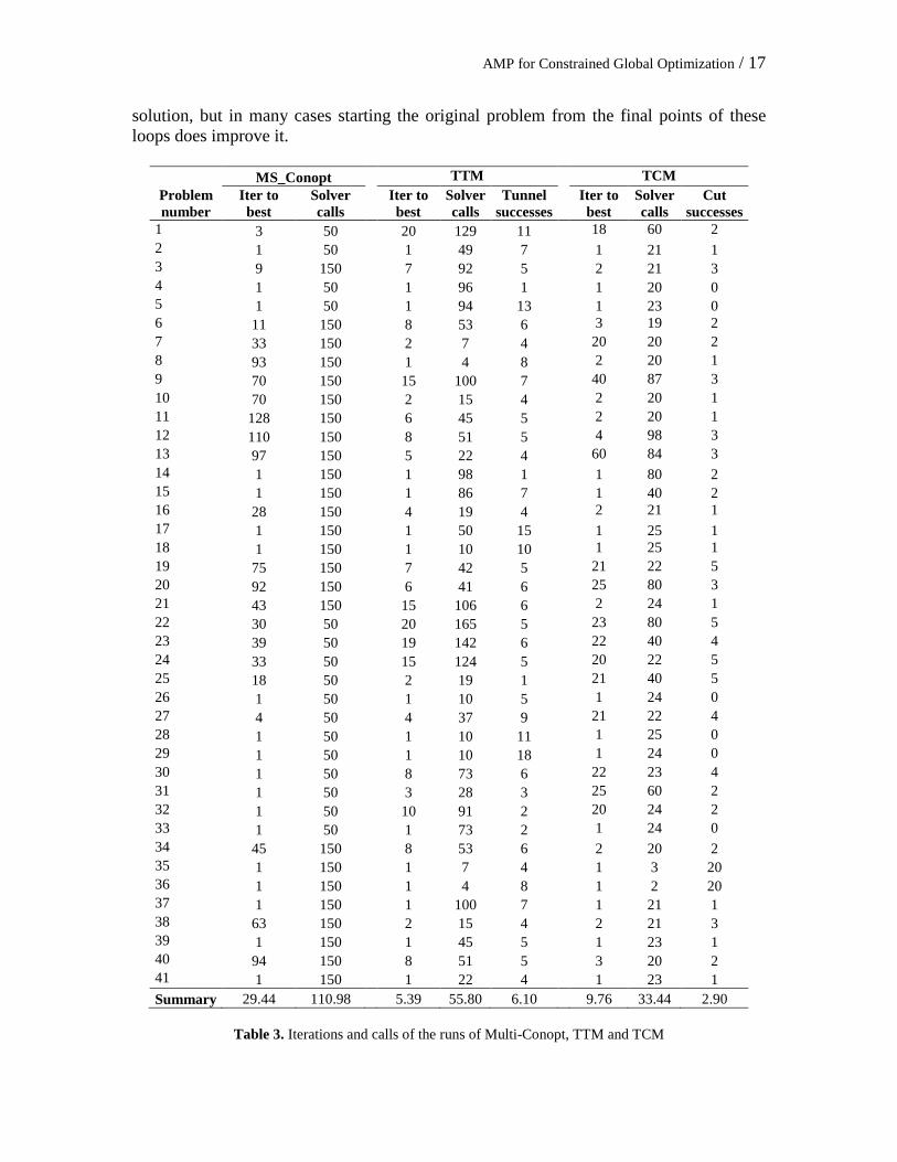
ending with a solution of the original problem, starting from the final point reached in the tunneling loop. In each tunneling loop the projection and tunneling subproblems are solved at most 4 times, fewer if the best value found so far is achieved or exceeded before 4 tunneling subproblems are solved. Each such occurrence is a tunneling “success”. Hence the local solver Conopt is called upon to find 21 solutions of the original problem (one at the user-provided initial point) and to solve at most 4*20 = 80 subproblems and 80 projection subproblems, at most 181 solver calls in all. Similarly, there are 20 cutting loops in the TCM, each one with the addition of at most 4 pseudo-cuts. Multi-Conopt is run with a CPU time limit similar to the TTM method (although the total time depends on the number of restarts and hence is adjusted indirectly). The Multi-start Conopt (MS-Conopt) performs very well when compared with the original Conopt method. MS-Conopt has a sum of the gaps of 187.08%, which compares favorably with the 1069.27% obtained by Conopt. Moreover, MS-Conopt is able to solve 33 out of the 41 problems shown in Table 2. The results obtained with these base runs of the TTM are encouraging, with 39 of the 41 problems solved to gaps of less than 1% and 37 solved to gaps of essentially zero. The total of the 41 gaps is 4.7%. On the other hand, the TCM obtains lower quality results when compared with TTM. It only solves 29 problems (with gaps of less than 1%) and exhibits a sum of gaps of 112.18%, which is smaller than the sum of gaps of MS-Conopt but considerably larger than the total gap obtained by TTM. Surprisingly, the largest gaps are obtained in problems belonging to the Ex2_1_7_n series, which the literature does not consider as hard as problems in the other series included in this set of test problems. However, it must be noted that the TCM is much faster than the other two methods. Specifically, MS-Conopt employs 117.31 seconds, TTM 140.15 while TCM consumes only 14.86 seconds. We have measured robustness (defined as the ability to yield high quality solutions consistently), by the standard deviation of the gap values, which for the experiments reported in Table 2 is 0.4% for TTM, 15.8% for MS-Conopt and 13.2% for TCM. The four problems (22-25) for which TTM obtained nonzero gaps are the largest of the EX8_6_1_n series. These problems have hundreds of local optima and are known to be very difficult for any global solver. The widely used multi-start solver OQNLP does not solve any of these problems to gaps of less than 1%, as we discuss momentarily. Table 3 complements the information in Table 2. The “Iter to best” and “Solver calls” columns show how quickly in the solution process the best solution is obtained in terms of the number of major iterations and the number of solver calls. The “successes” columns in TTM and TCM show the number of tunnel or pseudo-cut loop successes respectively, as defined above. The last row in Table 3 shows the average values for all these measures. Regarding computational efficiency, TTM finds its best solutions after roughly 1/3 of the major iteration budget of 20, averaging 6.9 major iterations to achieve its best solutions. The best solutions are found in 10 or fewer iterations in 20 of 26 problems. The average solver calls to best is 51.9, which is less than 25% of the maximum number of solver calls set at 221. An average of 6 tunneling loops out of 20 achieve an objective value at least as good as the best value discovered thus far, although some of these successes are revisits to the best known solution. Thus, most tunneling loops do not improve the best


solution, but in many cases starting the original problem from the final points of these loops does improve it.

MS_Conopt TTM TCM Problem number

Iter to best

Solver calls

Iter to best

Solver calls

Tunnel successes

Iter to best

Solver calls

Cut successes

1 3 50 20 129 11 18 60 2 2 1 50 1 49 7 1 21 1 3 9 150 7 92 5 2 21 3 4 1 50 1 96 1 1 20 0 5 1 50 1 94 13 1 23 0 6 11 150 8 53 6 3 19 2 7 33 150 2 7 4 20 20 2 8 93 150 1 4 8 2 20 1 9 70 150 15 100 7 40 87 3 10 70 150 2 15 4 2 20 1 11 128 150 6 45 5 2 20 1 12 110 150 8 51 5 4 98 3 13 97 150 5 22 4 60 84 3 14 1 150 1 98 1 1 80 2 15 1 150 1 86 7 1 40 2 16 28 150 4 19 4 2 21 1 17 1 150 1 50 15 1 25 1 18 1 150 1 10 10 1 25 1 19 75 150 7 42 5 21 22 5 20 92 150 6 41 6 25 80 3 21 43 150 15 106 6 2 24 1 22 30 50 20 165 5 23 80 5 23 39 50 19 142 6 22 40 4 24 33 50 15 124 5 20 22 5 25 18 50 2 19 1 21 40 5 26 1 50 1 10 5 1 24 0 27 4 50 4 37 9 21 22 4 28 1 50 1 10 11 1 25 0 29 1 50 1 10 18 1 24 0 30 1 50 8 73 6 22 23 4 31 1 50 3 28 3 25 60 2 32 1 50 10 91 2 20 24 2 33 1 50 1 73 2 1 24 0 34 45 150 8 53 6 2 20 2 35 1 150 1 7 4 1 3 20 36 1 150 1 4 8 1 2 20 37 1 150 1 100 7 1 21 1 38 63 150 2 15 4 2 21 3 39 1 150 1 45 5 1 23 1 40 94 150 8 51 5 3 20 2 41 1 150 1 22 4 1 23 1 Summary 29.44 110.98 5.39 55.80 6.10 9.76 33.44 2.90

Table 3. Iterations and calls of the runs of Multi-Conopt, TTM and TCM


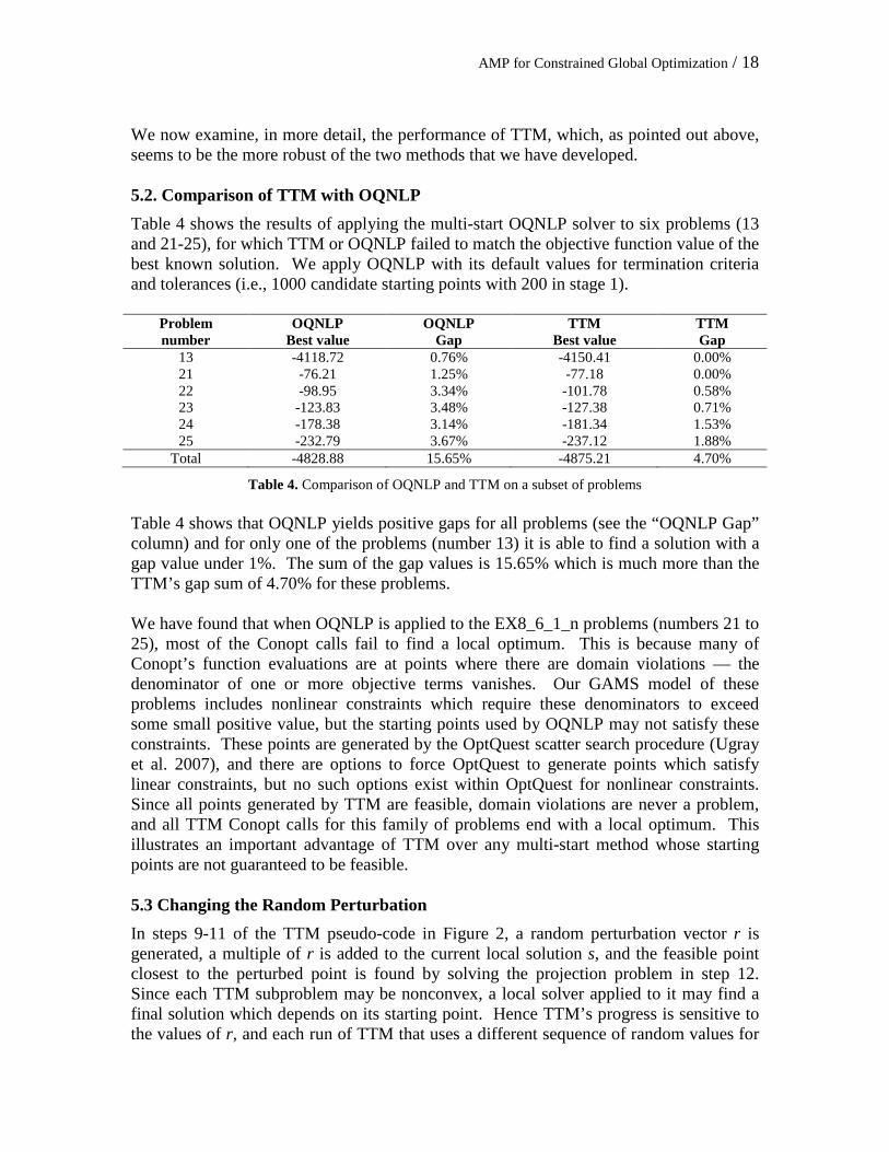
We now examine, in more detail, the performance of TTM, which, as pointed out above, seems to be the more robust of the two methods that we have developed. 5.2. Comparison of TTM with OQNLP Table 4 shows the results of applying the multi-start OQNLP solver to six problems (13 and 21-25), for which TTM or OQNLP failed to match the objective function value of the best known solution. We apply OQNLP with its default values for termination criteria and tolerances (i.e., 1000 candidate starting points with 200 in stage 1).

Problem number

OQNLP Best value

OQNLP Gap

TTM Best value

TTM Gap

13 -4118.72 0.76% -4150.41 0.00% 21 -76.21 1.25% -77.18 0.00% 22 -98.95 3.34% -101.78 0.58% 23 -123.83 3.48% -127.38 0.71% 24 -178.38 3.14% -181.34 1.53% 25 -232.79 3.67% -237.12 1.88%

Total -4828.88 15.65% -4875.21 4.70%

Table 4. Comparison of OQNLP and TTM on a subset of problems Table 4 shows that OQNLP yields positive gaps for all problems (see the “OQNLP Gap” column) and for only one of the problems (number 13) it is able to find a solution with a gap value under 1%. The sum of the gap values is 15.65% which is much more than the TTM’s gap sum of 4.70% for these problems. We have found that when OQNLP is applied to the EX8_6_1_n problems (numbers 21 to 25), most of the Conopt calls fail to find a local optimum. This is because many of Conopt’s function evaluations are at points where there are domain violations — the denominator of one or more objective terms vanishes. Our GAMS model of these problems includes nonlinear constraints which require these denominators to exceed some small positive value, but the starting points used by OQNLP may not satisfy these constraints. These points are generated by the OptQuest scatter search procedure (Ugray et al. 2007), and there are options to force OptQuest to generate points which satisfy linear constraints, but no such options exist within OptQuest for nonlinear constraints. Since all points generated by TTM are feasible, domain violations are never a problem, and all TTM Conopt calls for this family of problems end with a local optimum. This illustrates an important advantage of TTM over any multi-start method whose starting points are not guaranteed to be feasible. 5.3 Changing the Random Perturbation In steps 9-11 of the TTM pseudo-code in Figure 2, a random perturbation vector r is generated, a multiple of r is added to the current local solution s, and the feasible point closest to the perturbed point is found by solving the projection problem in step 12. Since each TTM subproblem may be nonconvex, a local solver applied to it may find a final solution which depends on its starting point. Hence TTM’s progress is sensitive to the values of r, and each run of TTM that uses a different sequence of random values for


r will generally differ from the others in the objective values found after each major and minor iteration, and in the best value found overall. The results shown in Tables 2 to 4 all used the same seed for the GAMS random number generator, so that the same results would be achieved if the problem were solved several times. Table 5 shows the results of changing the random number seed to 5 values, all different from each other and from the value used in Table 2, on two of the problems (13 and 22).

Problem number Run Final Obj Gap

Gap < 1% ?

Major iter to best

Solver calls

Tunnel successes

13 1 -4150.41 0.00% 1 5 28 4 2 -4150.41 0.00% 1 11 82 3 3 -4150.41 0.00% 1 5 26 6 4 -4023.94 3.05% 0 6 29 5 5 -4023.94 3.05% 0 13 100 4

22 1 -101.88 0.48% 1 20 163 7 2 -100.74 1.59% 0 15 118 5 3 -101.77 0.58% 1 11 78 5 4 -101.80 0.56% 1 2 9 2 5 -101.88 0.48% 1 5 34 2

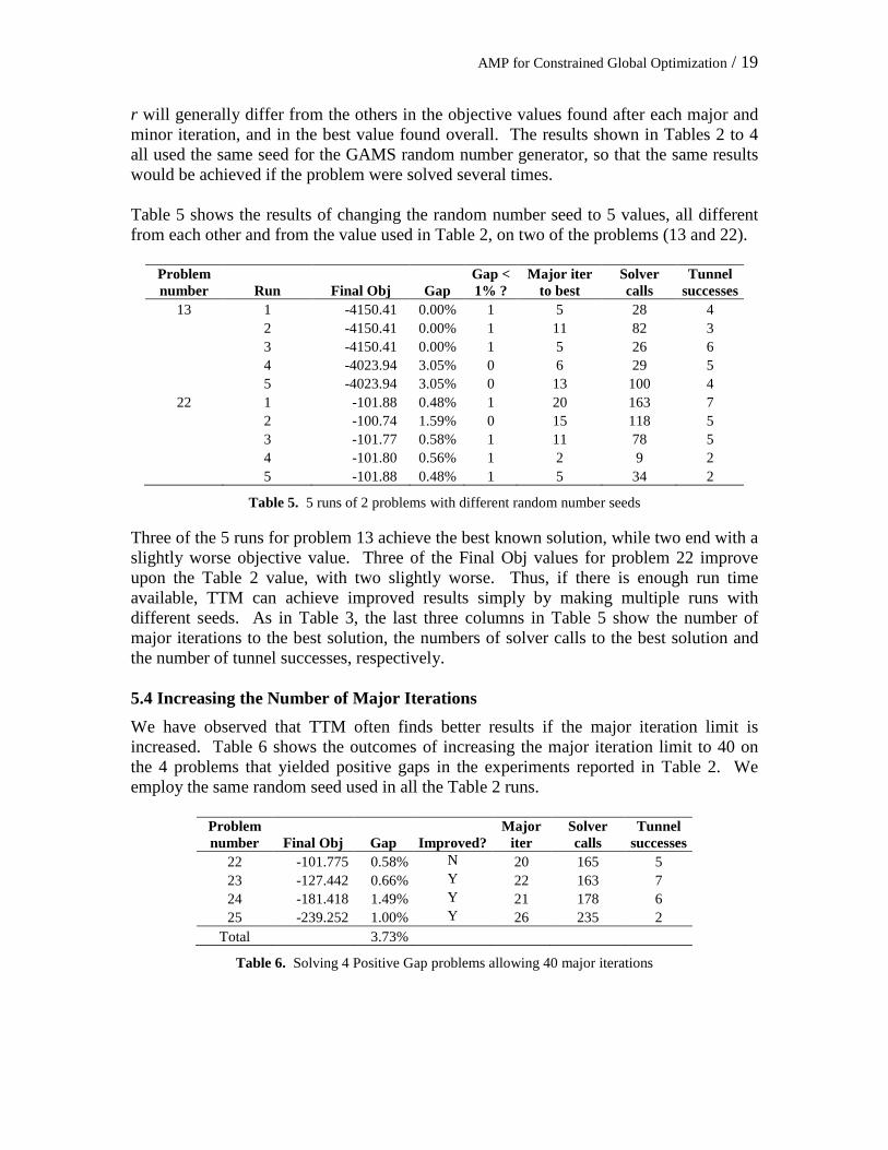
Table 5. 5 runs of 2 problems with different random number seeds Three of the 5 runs for problem 13 achieve the best known solution, while two end with a slightly worse objective value. Three of the Final Obj values for problem 22 improve upon the Table 2 value, with two slightly worse. Thus, if there is enough run time available, TTM can achieve improved results simply by making multiple runs with different seeds. As in Table 3, the last three columns in Table 5 show the number of major iterations to the best solution, the numbers of solver calls to the best solution and the number of tunnel successes, respectively. 5.4 Increasing the Number of Major Iterations We have observed that TTM often finds better results if the major iteration limit is increased. Table 6 shows the outcomes of increasing the major iteration limit to 40 on the 4 problems that yielded positive gaps in the experiments reported in Table 2. We employ the same random seed used in all the Table 2 runs.

Problem number Final Obj Gap Improved?

Major iter

Solver calls

Tunnel successes

22 -101.775 0.58% N 20 165 5 23 -127.442 0.66% Y 22 163 7 24 -181.418 1.49% Y 21 178 6 25 -239.252 1.00% Y 26 235 2

Total 3.73%

Table 6. Solving 4 Positive Gap problems allowing 40 major iterations


As shown in the “Improved?” column of Table 5, three of the four final objective values improve when increasing the number of major iterations from 20 to 40. The sum of the gaps is reduced from 4.70% to 3.73%.

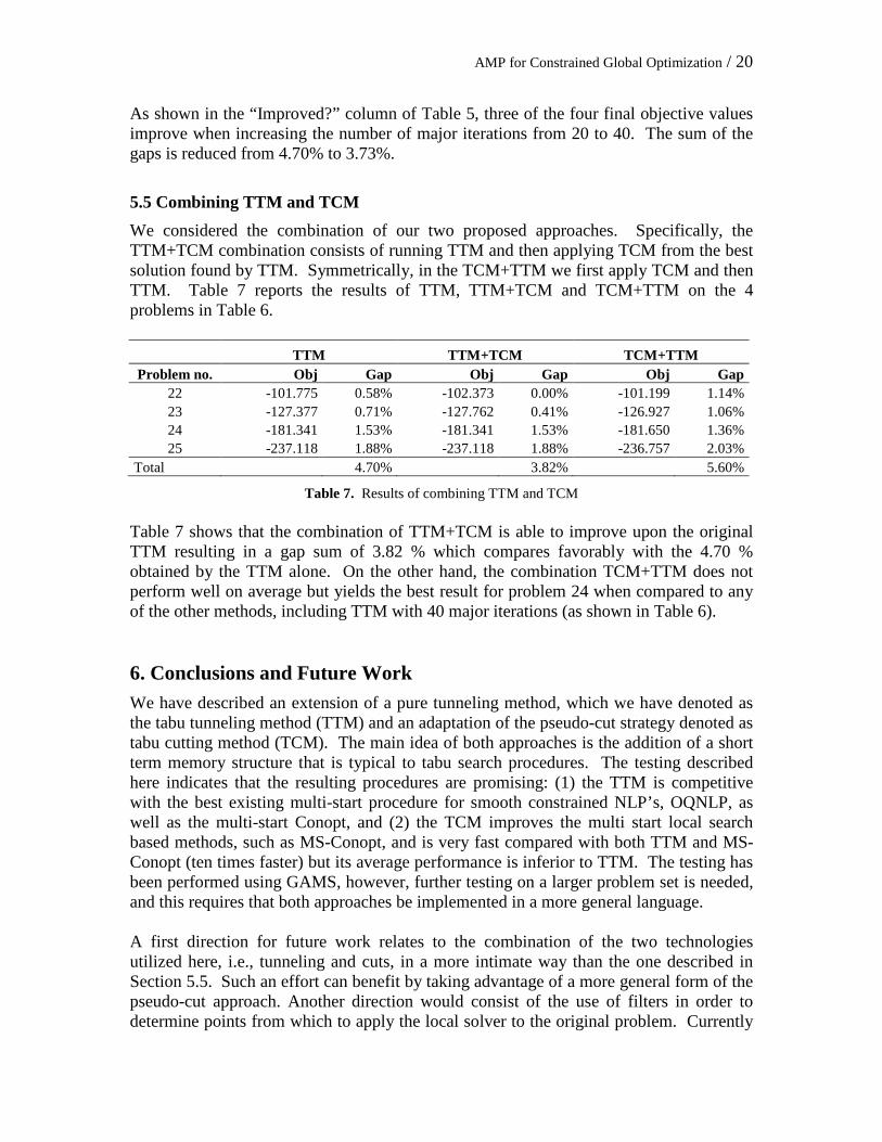
5.5 Combining TTM and TCM We considered the combination of our two proposed approaches. Specifically, the TTM+TCM combination consists of running TTM and then applying TCM from the best solution found by TTM. Symmetrically, in the TCM+TTM we first apply TCM and then TTM. Table 7 reports the results of TTM, TTM+TCM and TCM+TTM on the 4 problems in Table 6.

TTM TTM+TCM TCM+TTM Problem no. Obj Gap Obj Gap Obj Gap

22 -101.775 0.58% -102.373 0.00% -101.199 1.14% 23 -127.377 0.71% -127.762 0.41% -126.927 1.06% 24 -181.341 1.53% -181.341 1.53% -181.650 1.36% 25 -237.118 1.88% -237.118 1.88% -236.757 2.03%

Total 4.70% 3.82% 5.60%

Table 7. Results of combining TTM and TCM Table 7 shows that the combination of TTM+TCM is able to improve upon the original TTM resulting in a gap sum of 3.82 % which compares favorably with the 4.70 % obtained by the TTM alone. On the other hand, the combination TCM+TTM does not perform well on average but yields the best result for problem 24 when compared to any of the other methods, including TTM with 40 major iterations (as shown in Table 6). 6. Conclusions and Future Work We have described an extension of a pure tunneling method, which we have denoted as the tabu tunneling method (TTM) and an adaptation of the pseudo-cut strategy denoted as tabu cutting method (TCM). The main idea of both approaches is the addition of a short term memory structure that is typical to tabu search procedures. The testing described here indicates that the resulting procedures are promising: (1) the TTM is competitive with the best existing multi-start procedure for smooth constrained NLP’s, OQNLP, as well as the multi-start Conopt, and (2) the TCM improves the multi start local search based methods, such as MS-Conopt, and is very fast compared with both TTM and MS- Conopt (ten times faster) but its average performance is inferior to TTM. The testing has been performed using GAMS, however, further testing on a larger problem set is needed, and this requires that both approaches be implemented in a more general language. A first direction for future work relates to the combination of the two technologies utilized here, i.e., tunneling and cuts, in a more intimate way than the one described in Section 5.5. Such an effort can benefit by taking advantage of a more general form of the pseudo-cut approach. Another direction would consist of the use of filters in order to determine points from which to apply the local solver to the original problem. Currently


a solution found by solving a tunneling subproblem is used as a starting point for the original problem only if its objective value is at least as good as the best found so far, or if the iteration limit MaxIter (currently 5) is reached, in which case the last tunneling solution is used. TTM might be even more efficient if additional criteria were applied to determine whether or not to solve the original problem from one or more of the tunneling loop solutions. Following the ideas used in OQNLP, one might start from a tunneling solution whose true objective value was below a threshold — called the merit filter in Ugray et al. (2007) — and which was sufficiently far from any local solution of the original problem found so far (the distance filter). The merit filter criterion is applied in this version of TTM, with the threshold equal to the best objective value found thus far. However, a second more relaxed threshold could be used in conjunction with a distance filter, while exceeding the current threshold would terminate the tunneling loop unconditionally.

Acknowledgments This research has been partially supported by the Ministerio de Ciencia e Innovación of Spain (Grant Ref. TIN2006-02696, TIN2009-07516) and by the Comunidad de Madrid – Universidad Rey Juan Carlos project (Ref. URJC-CM-2008-CET-3731). References Alp, S., G. Ertek and S. Birbil (2006) “Application of the Cutting Stock Problem to a

Construction Company: A Case Study,” in Proceedings of the 5th International Symposium on Intelligent Manufacturing Systems, May 29-31, pp. 652-661.

April, J., M. Better, F. Glover, J. Kelly and M. Laguna (2006) “Enhancing Business Process Management with Simulation-Optimization,” in Proceedings of the 2006 Winter Simulations Conference, L. F. Perrone, F. P. Wieland, J. Liu, B. G. Lawson, D. M. Nicol, and R. M. Fujimoto (eds.), pp. 642-649.

Better, M., F. Glover and M. Laguna (2007) “Advances in Analytics: Integrating Dynamic Data Mining with Simulation Optimization,” IBM Journal of Research and Development, vol. 51, no. 3/4, pp. 477-487.

Conejo, A. J., E. Castillo, R. Minguez and R. Garcia-Bertrand (2006) Decomposition Techniques in Mathematical Programming, Springer, 541 pp.

Duarte, A., Martí, R., Glover, F. and Gortazar, F. (2009) “Hybrid Scatter Tabu Search for Unconstrained Global Optimization” Annals of Operations Research, forthcoming.

Drud, A. (1994) “CONOPT—A Large-Scale GRG-Code,” INFORMS Journal on Computing, vol. 6, no. 2, pp. 207-216.

Floudas, C.A., P.M. Pardalos, C.S. Adjiman, W.R. Esposito, Z. Gumus, S.T. Harding, J.L. Klepeis, C.A. Meyer and C.A. Schweiger (1999) Handbook of Test Problems for Local and Global Optimization, Springer, 484 pp.


Glover, F. (1989) “Tabu Search - Part I,” INFORMS Journal on Computing, vol. 1, no. 3, pp. 190-206.

Glover, F. (2008) “Pseudo-Cut Strategies for Global Optimization,” OptTek Systems, Inc., Technical Report.

Glover, F. and M. Laguna (1997) Tabu Search, Kluwer Academic Publishers: Boston, ISBN 0-7923-9965-X, 408 pp.

Levy, A.V. and S. Gomez (1985) “The Tunneling Method Applied to Global Optimization,” in Numerical Optimization, Boggs P. T., R. H. Byrd and R. B. Schnabel (eds.), SIAM, pp. 213-244.

Murray, W. and K-M. Ng (2002) “Algorithms for Global Optimization and Discrete Problems based on Methods for Local Optimization,” in Handbook of Global Optimization Volume 2, P. M. Pardalos and H. E. Romeijn (eds.), Springer, pp. 87-114.

Smith, S. and L. Lasdon (1992) “Solving Large Nonlinear Programs Using GRG,” INFORMS Journal on Computing, vol. 4, no. 1, pp. 2-15.

Ugray, Z., L. Lasdon, J. Plummer, F. Glover, J. Kelly and R. Martí (2007) “Scatter Search and Local NLP Solvers: A Multistart Framework for Global Optimization,” INFORMS Journal on Computing, vol. 19, no. 3, pp. 328-340.

adaptive memory programming for constrained …leeds-faculty.colorado.edu/glover/fred pubs/416 - amp...

Documents